Eclipses of continuous gravitational waves as a probe of stellar structure

Abstract

Although gravitational waves only interact weakly with matter, their propagation is affected by a gravitational potential. If a gravitational wave source is eclipsed by a star, measuring these perturbations provides a way to directly measure the distribution of mass throughout the stellar interior. We compute the expected Shapiro time delay, amplification and deflection during an eclipse, and show how this can be used to infer the mass distribution of the eclipsing body. We identify continuous gravitational waves from neutron stars as the best candidates to detect this effect. When the Sun eclipses a far-away source, depending on the depth of the eclipse the time-delay can change by up to $\sim 0.034~{}\mathrm{ms}$, the gravitational-wave strain amplitude can increase by $\sim 4\%$, and the apparent position of the source in the sky can vary by $4^{\prime\prime}$. Accreting neutron stars with Roche-lobe filling companion stars have a high probability of exhibiting eclipses, producing similar time delays but undetectable changes in amplitude and sky location. Even for the most rapidly rotating neutron stars, this time delay only corresponds to a few percent of the phase of the gravitational wave, making it an extremely challenging measurement. However, if sources of continuous gravitational waves exist just below the limit of detection of current observatories, next-generation instruments will be able to observe them with enough precision to measure the signal of an eclipsing star. Detecting this effect would provide a new direct probe to the interior of stars, complementing asteroseismology and the detection of solar neutrinos.

I Introduction

The subject of lensing of gravitational waves (GWs) was studied in the early 1970s and 1980s in the context of amplifying possible signals to the point of detection. This was in part driven by claims of the observation of GWs using cylindrical bar detectors Weber (1969), for which the reported amplitude was too high to be explained by astrophysical sources. Considering the Galactic core as a lens, it was shown that this was insufficient to explain those detections Lawrence (1971); Ohanian (1973). Lensing by the Sun was also shown to be unimportant for the observation of GWs, as diffraction effects imply that a significant amplification of the signal is only expected for GWs with frequencies $>10^{4}~{}\mathrm{Hz}$ Ohanian (1973); Bontz and Haugan (1981); Ohanian (1983). This is higher than the frequencies of known astrophysical GW sources, which are not expected to exceed a few kilohertz Kokkotas (2008). Currently, strong lensing is only expected to affect a small number of observable sources of GWs Smith et al. (2018); Ng et al. (2018); Li et al. (2018), and there is no strong evidence for current detections having been strongly lensed Hannuksela et al. (2019). Microlensing of GWs is also considered to be an unlikely event, but owing to the relatively low frequencies of GW sources can lead to wave-optical phenomena that allow the inference of additional information about the lens Takahashi and Nakamura (2003); Moylan et al. (2008); Liao et al. (2019).

Even if GW lensing is not expected to play a role in the majority of observable sources, measuring small effects of intervening matter on GWs can provide interesting astrophysical information. The detection of GWs from merging binary black holes (BHs) Abbott et al. (2016, 2019a) and neutron stars (NSs) Abbott et al. (2017a, 2019a) by the Advanced LIGO Aasi et al. (2015) and Virgo Acernese et al. (2015) detectors makes it possible to use them as astrophysical tools. In particular, GWs crossing the interior of a star carry information on its internal mass distribution. For instance, it has been proposed that measuring the deflection angle of a GW source eclipsed by the Sun will yield the solar density profile Cyranski and Lubkin (1974).

In this paper we discuss the effects of eclipsing stars on GWs, and how these provide information on the interior of the eclipsing star. Our focus is on high-frequency ($>1$ Hz) GWs that are potentially detectable by ground-based observatories. In Section II we discuss different sources of GWs that could be used for this purpose, and show that high-frequency continuous GWs (CWs) work best. In Section III we analyze the effects produced on high-frequency GWs crossing the interior of the Sun using both geometric and wave optics, while in Section IV we discuss the case where the eclipsing star is a binary companion to the source of GWs. We explore the detectability of these effects in Section V, and give our conclusions in Section VI. All code used to produce figures and compute our results is available at .

II Continuous GWs or compact binary coalescences

Although only GWs from compact binary coalescences (CBCs) have been directly detected to date Abbott et al. (2019a), these sources are not useful for extracting information from an eclipsing event. If we are interested in observing a source behind the Sun, the probability of observing this for a CBC (assuming they are isotropically distributed) is given by the fraction of the sky that is covered by the solar disk which has an angular diameter of $\sim 32^{\prime}$. This is because such sources pass quickly through the ground-based detector band, and during this time the position of the Sun is essentially static. The probability of it being located behind the Sun is then just $0.00054\%$, and even after $10^{4}$ observations, there’s only a $5.3\%$ chance that at least one source is eclipsed.

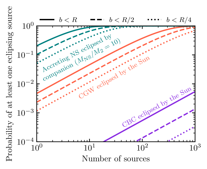
Figure 1: Probability of observing at least one eclipsing source as a function of the number of observed sources. Colors indicate different types of sources, while line styles indicate the depth of the eclipse. For the case of CBCs and CWs eclipsed by the Sun, probabilities are computed assuming an isotropic distribution in the sky, and an observer on Earth. Probabilities for the case of an accreting NS being eclipsed by its companion are computed assuming a mass ratio $q\equiv M_{\mathrm{NS}}/M_{2}=10$ and by approximating the stellar companion as a sphere with a radius equal to its Roche lobe.

.

Even if an eclipsing CBC is detected to high precision, it is difficult to distinguish effects inherent to the source from those produced by the eclipsing star in the absence of previous information about the source. GW signals from a CBC source are short-lived in the LIGO–Virgo band (a binary neutron star evolves form a GW frequency of 10 Hz to merger in less than 20 minutes) relative to the duration of an eclipse; this makes it implausible to compare the signal of an eclipsed source against its pre- or post-eclipse signal.

On the other hand, CWs are ideal for this purpose as any source located $\lesssim 16^{\prime}$ from the ecliptic and lasting more than a year will be eclipsed by the Sun. The probability of a single source undergoing an annual eclipse (assuming an isotropic distribution) is $0.47\%$, and with $200$ sources the probability that at least one will undergo an eclipse is $61\%$ (see Fig. 1). The likelihood of this happening is actually larger; unlike CBCs, many expected sources of CWs are Galactic, thus not isotropically distributed in the sky, and the Sun crosses the Galactic bulge. Moreover, a CW can be studied and characterized before a lensing event, making it easier to extract information from an eclipse.

In terms of expected sources of CWs, binary white dwarfs will be a prime source for the LISA observatory Amaro-Seoane et al. (2017), with known sources predicted to be detectable given the design sensitivity of the instrument Stroeer and Vecchio (2006); Kupfer et al. (2018). However, the wavelengths of these sources are larger than the Sun, as are the arms of the LISA constellation itself. Any effects produced by the Sun on such long-wavelength sources are small due to diffraction. As we show later, signals with GW frequencies below $10~{}\mathrm{Hz}$ are essentially unperturbed by the Sun.

Rotating NSs are potential sources of high-frequency CWs Prix (2009); Riles (2017); a NS with a non-zero quadrupolar moment is expected to emit GWs at a frequency $f_{\rm GW}=2\nu$, where $\nu$ is the rotational frequency of the NS Zimmermann and Szedenits (1979). For known pulsars with measured time derivatives, a rough upper limit on the strength of emitted GWs can be obtained by assuming its spin-down is solely due to energy emitted in GWs. The latest searches for isolated sources using data from the first and second observing runs of Advanced LIGO, have not resulted in a detection Abbott and et al. (2019a, b, c). However, the searches made for known pulsars Abbott and et al. (2019a, b) have further increased the sample of young pulsars for which the spin-down limit is reached to $20$, and are within factors of a few of the spin-down limit for some millisecond pulsars (MSPs).

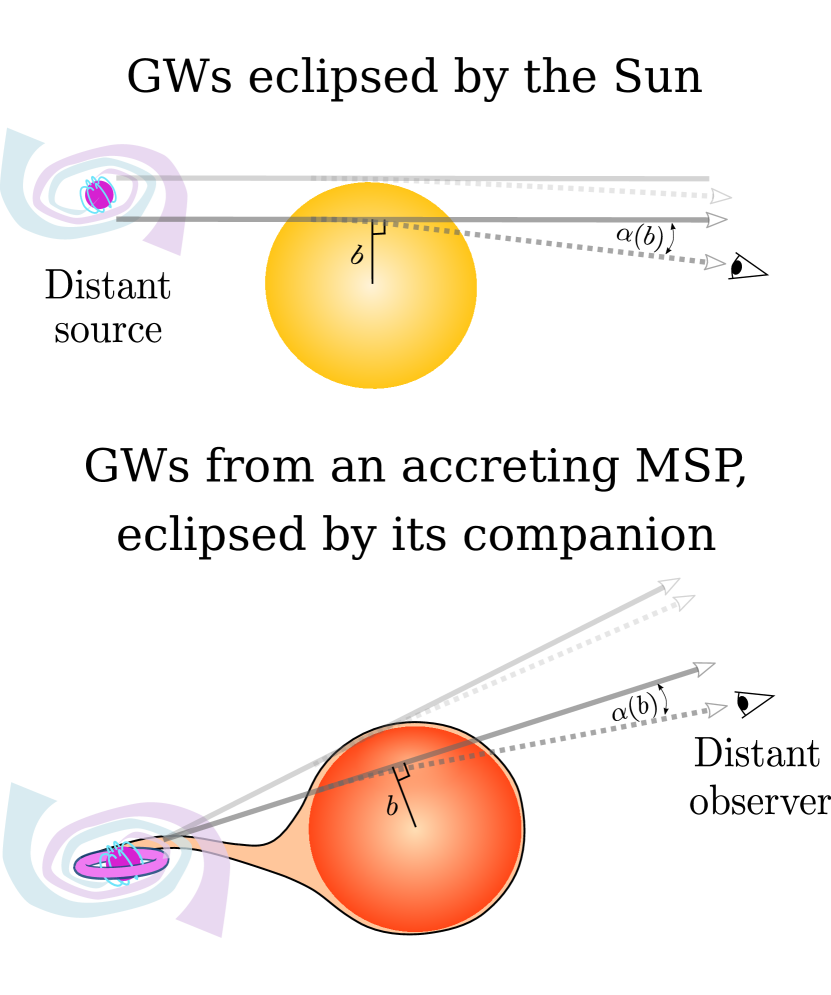
Figure 2: Two different types of eclipses that could allow the measurement of the internal mass distribution of stars. (top) Eclipse of a distant GW source by the Sun, observed at Earth. In this case, all rays approaching the Sun are essentially parallel to each other, resulting in caustics far from Earth. (bottom) GWs from an accreting NS eclipsed by its companion.

.

Accreting millisecond X-ray pulsars (AMXPs) with a Roche-lobe filling companion are expected to be particularly strong sources of high-frequency CWs. These objects are believed to reach a point where accretion spin-up is compensated by energy losses from the emission of GWs Wagoner (1984); Bildsten (1998), which could also result from the excitation of the r-mode instability Haskell (2015). Moreover, systems undergoing Roche lobe overflow have a high probability that the compact object is eclipsed by its companion (see Fig. 2 and Fig. 1). For a system with a mass ratio $q\equiv M_{\rm NS}/M_{2}=10$, the probability that it undergoes eclipses is $\sim 20\%$, and in particular there is one known eclipsing AMXP, SWIFT J1749.4$-$2807 Markwardt and Strohmayer (2010).

As depicted in Fig. 2, there are two different situations of interest. If GWs cross the Sun, then by measuring them we could extract information about the solar interior. Meanwhile, if the eclipsing source is the companion star of an accreting MSP, GWs provide a probe into the mass distribution of the companion. Eclipses by the Sun would happen annually and last at most 12 hours, while eclipses from the companion of an accreting source would happen every orbit, and could last for more than 10% of the orbital period depending in the orbital inclination and the mass ratio.

Table 1: Known pulsars with rotational frequencies $>10$ Hz and accreting neutron stars near the ecliptic.

Source	note	$\nu$ $[\rm Hz]$	ecliptic latitude	reference
J1022+1001	MSP	60.8	$-0.064^{\circ}$	Reardon et al. (2016)
J1730$-$2304	MSP	123	$0.19^{\circ}$	Reardon et al. (2016)
J1142+0119	MSP	197	$-0.58^{\circ}$	Ray et al. (2012)
J1646$-$2142	MSP	171	$0.65^{\circ}$	Ray et al. (2012)
The Crab pulsar	young pulsar	29.9	$1.3^{\circ}$	Lyne et al. (2015)
Sco X-1	accreting NS	-	$5.5^{\circ}$	Bradshaw et al. (1999)
XTE J1751$-$305	accreting MSP	435	$-7.2^{\circ}$	Markwardt et al. (2002)
SWIFT J1749.4$-$2807	accreting, eclipsing MSP	518	$-4.7^{\circ}$	Ferrigno et al. (2011)

In Table 1 we summarize a few known sources of interest. From the ATNF pulsar catalogue Manchester et al. (2005) we find two recycled millisecond pulsars (MSPs) that are eclipsed by the Sun, J1022+1001 and J1730$-$2304. MSPs are stable clocks (cf. Manchester (2004)), such that timing of GWs and measurement of the Shapiro delay Shapiro (1964) during an eclipse might be possible. MSPs have low spin-down limits, and Advanced LIGO and Virgo at design sensitivity are not guaranteed to detect either of these sources Abbott and et al. (2019a). In contrast, the spin-down limit has been reached for the Crab pulsar Aasi et al. (2014), but it is not eclipsed by the Sun. Young pulsars also exhibit sudden frequency shifts called glitches Espinoza et al. (2011) which make timing of the signal difficult for extended periods of time. But even for prolific glitchers like the Crab there have not been two glitches detected less than 10 days apart from each other Lyne et al. (2015), making the likelihood of a glitch happening during an eclipse small. Six more pulsars from the ATNF catalogue are eclipsed by the Sun, but their low frequencies ($\nu<10~{}\mathrm{Hz}$) make them unsuitable.

Sco X-1 and XTE J1751$-$305 are two AMXPs which are close to the ecliptic, though not close enough to be eclipsed by the Sun. Searches of the first and second observing runs of Advanced LIGO have provided upper limits on potential GW emission from Sco X-1 Abbott et al. (2017b, c, 2019b), and searches of initial LIGO data have provided upper limits for XTE J1751$-$305 Meadors et al. (2017). SWIFT J1749.4$-$2807 is also an AMXP, and a particularly interesting source because it undergoes periodic eclipses from its companion. The number of AMXPs has grown significantly in the last decade Patruno and Watts (2012). Although none of the 19 AMXPs known so far are eclipsed by the Sun, it is likely that an eclipsing source will be found with further detections. This is particularly relevant, as AMXPs are a favoured candidate for the first detection of high-frequency GWs Lasky (2015).

III Effects of the Sun on eclipsed GWs

We consider the impact of three different effects. As a GW signal passes near the Sun, it experiences gravitational deflection, which also impacts the apparent luminosity of the source. In addition, the time of arrival of signals is delayed compared to what would happen if the Sun was absent, which constitutes the Shapiro delay Shapiro (1964). We first use geometrical optics to compute these effects as observed from the Earth, and then perform wave optics calculations to check at which frequencies geometric optics is a good approximation. We use a $1M_{\odot}$ model computed until an age of $4.57\,{\rm Gyr}$ Bahcall et al. (1995) with the MESA Paxton et al. (2011, 2013, 2015, 2018) code (version r10398) to represent the Sun, and all calculations assume a radial mass distribution. Although our model is not calibrated to constraints from asteroseismic or neutrino measurements of the Sun, it matches the mass profile $m(r)$ of the calibrated solar models computed by Vinyoles et al. (2017) to within $2\%$.

The Earth is located far from the caustics produced by the solar lens, and in its neighborhood the predicted perturbations to the waveform vary on lengthscales of the order of $R_{\odot}$. We then expect the geometric optics approximation to apply for $\lambda\ll R_{\odot}$, which is the case for rapidly rotating NSs that emit GWs at frequencies above $1000~{}\mathrm{Hz}$.

III.1 Deflection and amplification

The deflection and amplification produced by a spherically symmetric gravitational lens are well known results of lensing theory (cf. Clark (1972)). The deflection angle can be obtained in terms of the distance of closest approach $b$, and the mass contained within an infinite cylinder of radius $b$ centered at the lens, $M_{\rm cyl}(b)$. For the Sun, the deflection angle is

$$\alpha(b)=\frac{4GM_{\rm cyl}(b)}{c^{2}b}=1.75^{\prime\prime}\frac{M_{\rm cyl}(b)}{M_{\odot}}\left(\frac{b}{R_{\odot}}\right)^{-1},$$ (1)

and $M_{\rm cyl}(b)$ can be computed from a spherically symmetric density profile $\rho(r)$ and spherical mass coordinate $m(r)$ as

$$\begin{aligned} M_{\rm cyl}(b)=m(b)\qquad\qquad\qquad\qquad\qquad\qquad\qquad\\ +4\pi\int_{b}^{R_{\odot}}\rho(r)r^{2}\left(1-\sqrt{1-\frac{b^{2}}{r^{2}}}\right)\mathrm{d}r.\end{aligned}$$ (2)

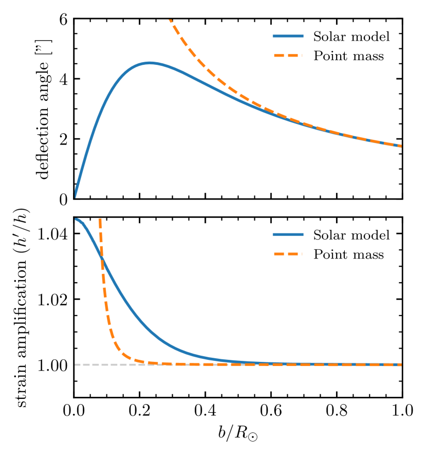
Figure 3: (top) Deflection $\alpha$ of a GW as a function of its distance of closest approach to the center of the Sun. (bottom) Amplification of the GW strain as a function of its distance of closest approach to the center of the Sun, considering a detector located at the Earth. In both panels, the dashed line indicates the corresponding effect if the Sun were a point mass.

Figure 3 shows the expected effect from a detailed solar model, showing that the maximum angle of deflection is smaller than $5^{\prime\prime}$. An observer does not measure this angle directly, but instead detects an angular variation $\Delta\theta$ for the location of the source in the sky. Defining the optical axis as the line joining the center of the lens and the source, and the optical plane as the plane perpendicular to the optical axis that crosses the lens, we approximate the effect of the lens as simply kinking an incoming ray by an angle $\alpha(b)$ at the optical plane (see Fig. 4). In addition, $b$ is approximated as the distance of closest approach of the undeflected ray. This is a standard approximation that is justified when the deflection angle $\alpha$ is small Refsdal (1964). Under these assumptions we have that

$$\Delta\theta=\alpha\sqrt{\frac{d_{ls}^{2}+b^{\prime 2}}{l^{2}+(d_{ls}+d_{l})^{2}}},$$ (3)

where we have assumed $\Delta\theta$ and $\alpha$ are small angles, $d_{ls}$ is the distance between the source and the lens and $d_{l}$ is the distance between the source and the observer along the optical axis. The distance between the center of the lens and the point where the undeflected ray would intersect the optical plane is denoted by $b^{\prime}$, while the distance between the observer and the optical axis is denoted as $l$. The values of $b^{\prime}$ and $l$ can be computed as

$$b^{\prime}=\frac{bd_{ls}}{\sqrt{d_{ls}^{2}-b^{2}}},\qquad l=\frac{d_{ls}+d_{l}}{d_{ls}}b^{\prime}-d_{l}\alpha(b).$$ (4)

Considering a distant source lensed by the Sun and observed from Earth, $d_{ls}\gg d_{l}$ and $d_{ls}\gg l$, such that Eq. (3) results in $\Delta\theta\simeq\alpha$ (i.e. the deflection angle is equal to the apparent change in location of the source). Measuring this deflection angle would provide a direct measurement of the solar mass distribution Cyranski and Lubkin (1974).

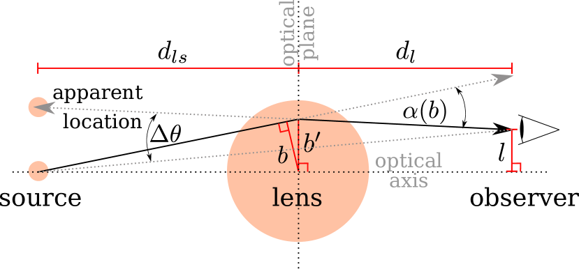
Figure 4: Definition of variables used to compute the change in sky location and amplification of signals from the solar lens. The deflection angle is greatly exaggerated.

The change in strain is equal to the square root of the change in luminosity. Following Fig. 4 and applying the geometrical optics approximation results in Clark (1972)

$$\frac{h^{\prime}(b)}{h}=\left(\frac{d_{ls}+d_{l}}{d_{ls}}\right)\sqrt{\frac{b^{\prime}}{l}}\left(\frac{d_{ls}+d_{l}}{d_{ls}}-d_{l}\frac{\mathrm{d}\alpha}{\mathrm{d}b}\right)^{-1/2},$$ (5)

where $h$ is the strain that would be measured in the absence of lensing. For the case of a distant source being lensed by the Sun $d_{ls}\gg d_{l}$ and $b^{\prime}$ is almost equal to $b$, leading to

$$\frac{h^{\prime}(b)}{h}=\left(\frac{b}{b-a_{\oplus}\alpha(b)}\right)^{1/2}\left(1-a_{\oplus}\frac{\mathrm{d}\alpha}{\mathrm{d}b}\right)^{-1/2},$$ (6)

where $d_{l}=a_{\oplus}=1\;\rm au$. The result from our solar model is shown in Fig. 3. The maximum amplification, which happens at the core of the Sun, is a factor $1.043$ of the non-lensed strain. In contrast, a point mass results in no amplification during most of an eclipse, with a steep rise below $b/R_{\odot}\sim 0.1$. The large deflection angles that would be produced by a point mass result in rays with $b/R_{\odot}\sim 0.05$ focusing at $1$ au from the Sun, at which point the geometric optics approximation is not valid.

III.2 Shapiro delay

The time delay of a signal as it passes by the Sun, compared to the arrival time the signal would have in the absence of the Sun, is given by Shapiro (1964); Backer and Hellings (1986)

$$\Delta t=-\frac{2}{c^{3}}\int_{A}^{B}\Phi\,\mathrm{d}l,$$ (7)

where $A$ and $B$ denote the location of the source and the receiver, and $\Phi$ is the gravitational potential of the Sun which satisfies Poisson’s equation $\nabla^{2}\Phi=4\pi G\rho$ and, assuming spherical symmetry for the Sun, is given by $\Phi=-GM_{\odot}/r$ for $r>R_{\odot}$. Equation (7) is given in coordinate time, and the actual time delay measured on Earth includes additional small corrections that depend on the Solar System ephemerides Backer and Hellings (1986). The integral in Eq. (7) can be estimated by integrating through the straight line path that the unperturbed light ray would follow, as the additional delay produced by the deflection of the null geodesic only adds up to a few tens of nanoseconds Richter and Matzner (1983). If the trajectory does not go through the Sun, then Eq. (7) is equal to

$$\Delta t_{\rm out}=-\frac{2GM_{\odot}}{c^{3}}\ln\left(\frac{\hat{n}\cdot\vec{a}_{\oplus}+a_{\oplus}}{\hat{n}\cdot\vec{a}_{\rm s}+a_{\rm s}}\right),$$ (8)

where $\vec{a}_{\rm s}$ and $\vec{a}_{\rm\oplus}$ are the positions of the source and the receiver with respect to the Sun, and $\hat{n}$ is a unit vector from the receiver to the source. If the source is far away, such that $\hat{n}\cdot\vec{a}_{\rm s}+a_{\rm s}\simeq 2a_{\rm s}$, the time delay can be approximated as

$$\Delta t_{\rm out}=-\frac{2GM_{\odot}}{c^{3}}\ln\left[\frac{a_{\oplus}}{2a_{\rm s}}(1-\cos\beta)\right],$$ (9)

where $\beta$ is the angle in the sky between the center of the Sun and the source, as observed from the location of the receiver ($\cos\beta=-\hat{n}\cdot\vec{a}_{\oplus}/a_{\oplus}$). For sources close to the solar disk $\beta$ is small, such that the time delay can be expressed in terms of the distance of closest approach to the Sun $b\simeq\beta a_{\oplus}$,

$$\Delta t_{\rm out}{(b)}=-\frac{4GM_{\odot}}{c^{3}}\ln\left(\frac{b}{2\sqrt{a_{\oplus}a_{\rm s}}}\right).$$ (10)

If the line does go through the Sun, then this equation has to be corrected for the part of the trajectory that crosses it,

$$\Delta t{(b)} = \Delta t_{\rm out}{(b)}-\Delta t_{-}{(b)}+\Delta t_{+}{(b)},$$ (11)

$$\Delta t_{-}{(b)} = \frac{2}{c^{3}}\int_{A^{\prime}}^{B^{\prime}}\frac{GM_{\odot}}{r}\,\mathrm{d}l,$$ (12)

$$\Delta t_{+}{(b)} = {-}\frac{2}{c^{3}}\int_{A^{\prime}}^{B^{\prime}}\Phi(r)\,\mathrm{d}l,$$ (13)

where $A^{\prime}$ and $B^{\prime}$ are the points where the trajectory crosses the surface of the Sun. Computing $\Delta t_{-}$ yields

$$\Delta t_{-}{(b)}=-\frac{4GM_{\odot}}{c^{3}}\ln\left(\frac{b}{R_{\odot}+\sqrt{R_{\odot}^{2}-b^{2}}}\right),$$ (14)

while $\Delta t_{+}$ can be transformed into an integral over the mass coordinate of the Sun,

$$\Delta t_{+}{(b)} = -\frac{4}{c^{3}}\int_{b}^{R_{\odot}}\frac{\Phi(r)r}{\sqrt{r^{2}-b^{2}}}\,\mathrm{d}r$$ (15)

$$= \frac{4GM_{\odot}}{c^{3}}\frac{\sqrt{R_{\odot}^{2}-b^{2}}}{R_{\odot}}$$

$$+\left.\frac{4}{c^{3}}\int_{b}^{R_{\odot}}\frac{Gm(r)}{r^{2}}\sqrt{r^{2}-b^{2}}\,\mathrm{d}r\right.,$$

where we have used $\mathrm{d}\Phi/\mathrm{d}r=Gm(r)/r^{2}$ and $\Phi(R_{\odot})=-GM_{\odot}/R_{\odot}$. Since only relative changes in the arrival time of pulses can be determined, it is more useful to consider the difference between the delay time for $b$, and the delay time of a signal that passes right by the surface of the Sun ($b=R_{\odot}$). Combining Eq. (10), (13), (14) and (15) then gives us the time delay as a function of $b$ and the mass profile of the Sun $m(r)$,

$$\Delta t(b)-\Delta t(R_{\odot})=-\frac{4GM_{\odot}}{c^{3}}\qquad\qquad\qquad\qquad$$

$$\times\left[\ln\left(\frac{R_{\odot}+\sqrt{R_{\odot}^{2}-b^{2}}}{R_{\odot}}\right)-\frac{\sqrt{R_{\odot}^{2}-b^{2}}}{R_{\odot}}\right.$$

$$\left.-\frac{1}{M_{\odot}}\int_{b}^{R_{\odot}}\frac{m(r)}{r^{2}}\sqrt{r^{2}-b^{2}}\,\mathrm{d}r\right].$$ (16)

This can be rewritten in a way that clearly distinguishes the contribution for the case of a point mass,

$$\Delta t(b)-\Delta t(R_{\odot})=-\frac{4GM_{\odot}}{c^{3}}\left[\ln\left(\frac{b}{R_{\odot}}\right)\right.\qquad\qquad$$

$$\left.{+}\frac{1}{M_{\odot}}\int_{b}^{R_{\odot}}\frac{M_{\odot}-m(r)}{r^{2}}\sqrt{r^{2}-b^{2}}\,\mathrm{d}r\right].$$ (17)

The factor $4GM_{\odot}/c^{3}=0.02~{}\mathrm{ms}$ shows how small the expected effect is. The time delay is plotted in Fig. 5, and the largest delay is of $\sim 0.034~{}\mathrm{ms}$ for a source crossing the center of the Sun. This represents a shift in the phase of the pulsars listed in Table 1 ranging from a half of a percent to a few percent. When the source is not eclipsed the Shapiro delay still changes depending on the angle $\beta$ between the locations of the source and the Sun in the sky. Combining Eq. (9) and Eq. (10) and considering a source located on the opposite side of the sky from the Sun ($\beta=\pi$) results in

$$\begin{aligned} \Delta t(\beta=\pi)-\Delta t(R_{\odot})&=-\frac{4GM_{\odot}}{c^{3}}\ln\left(\frac{2a_{\oplus}}{R_{\odot}}\right)\\ &=-0.12~{}\mathrm{ms}.\end{aligned}$$ (18)

The magnitude of this orbital variation in the time delay is larger than that during an eclipse, but it can only provide information on the total mass of the Sun rather than its internal structure.

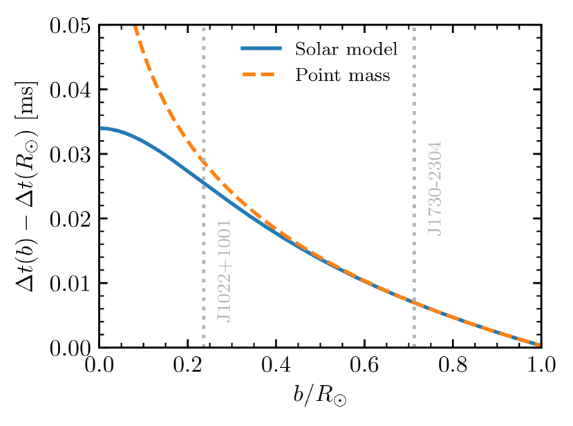
Figure 5: The time delay imprinted on a GW as a function of its distance of closest approach to the center of the Sun. The solid line shows the delay derived from a detailed solar model computed with the MESA code, while the dashed line is the effect from a point mass and represents an absolute upper limit. The two dotted vertical lines indicate the lowest value of $b$ reached by the two known MSPs that are eclipsed by the Sun.

Equation (17) provides information on the solar interior in the form of an integral over the mass distribution. If the derivative of the time delay as a function of $b$ can be measured as the source passes behind the Sun, it provides a direct measurement of $M_{\rm cyl}(b)$,

$$\frac{\mathrm{d}\Delta t}{\mathrm{d}b}=-\frac{4GM_{\rm cyl}(b)}{c^{3}b}=-\frac{\alpha(b)}{c}.$$ (19)

This relation between the deflection angle and the time delay is exactly what is expected in terms of the change in direction of propagation of an incoming wavefront.

III.3 Wave optics

Calculations using geometric optics are only valid in the limit that the effects of the lens on the amplitude, phase, and direction of propagation of a wave occur on lengthscales much larger than a wavelength, and on timescales much longer than the period of the wave. For the case of an eclipse by the Sun being observed at Earth, all predicted effects on incoming waves are small and operate on a lengthscale $\sim R_{\odot}$, such that the geometric optics approximation requires $\lambda\ll R_{\odot}$. The timescale on which the properties of the wave change corresponds to the duration of the eclipse $\tau_{\rm ec}$, which sets a limit on the frequency of the source for the applicability of geometric optics, $f_{\rm GW}^{-1}\ll\tau_{\rm ec}$. The tighter constraint is provided by the limit on the wavelength; for $\lambda=R_{\odot}$ the corresponding frequency is $f_{\rm GW}\sim 0.5~{}\mathrm{Hz}$, so the geometric optics approximation requires $f_{\rm GW}\gg 0.5~{}\mathrm{Hz}$. This implies that our geometric optics calculations are only applicable in the high-frequency range that is probed by ground based observatories, while at lower frequencies the impact of wave optics needs to be analyzed with care.

For practical purposes, it is necessary to quantify how much smaller than $R_{\odot}$ the wavelength needs to be for wave optics effects to become negligible. For this, we need to drop the assumption of geometric optics. Following Ohanian (1974); Bontz and Haugan (1981), we compute the Kirchhoff integral, which allows the calculation of a wave given its properties on a surface surrounding the observation point. The effect of the lens is encoded by the time delay given by Eq. (17), which produces a phase shift at the lens plane. Given this, the Kirchhoff integral can be numerically computed to determine the amplification and the time delay observable at any point in space (see Appendix A).

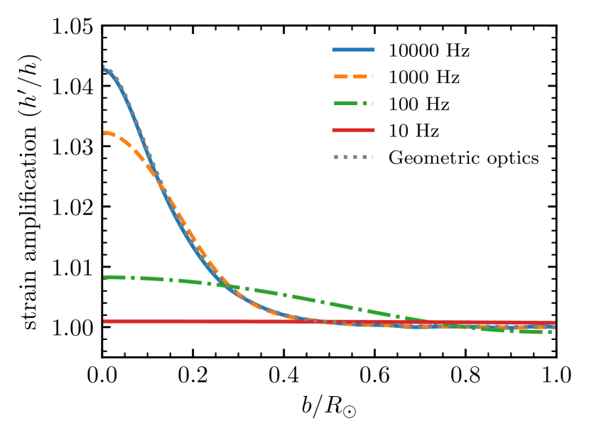
Figure 6: Amplification of the GW strain observable at Earth during an eclipse. Each line indicates a different frequency, while the geometric optics result is the expected value in the limit that $f_{\rm GW}\rightarrow\infty$.

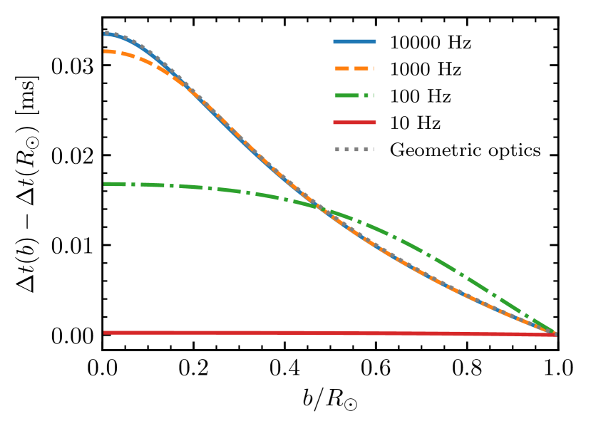
Figure 7: Time delay observable at Earth during an eclipse. Each line indicates a different GW frequency; the geometric optics result is the expected value in the limit that $f_{\rm GW}\rightarrow\infty$.

Using our solar model, we compute the amplitude and time delays observable at Earth through an eclipse for sources at different frequencies, which we show together with the expected results from geometric optics in Fig. 6 and 7. As expected, at frequencies below 10 Hz the amplification and the time delay are negligible, meaning that waves with that frequency are unaffected by the solar lens. At $100~{}\mathrm{Hz}$ the solar lens can amplify a signal by up to $\sim 1\%$, and delay it by $\sim 0.02\,{\rm ms}$, but it still deviates significantly from the geometric optics calculation. At $10^{3}~{}\mathrm{Hz}$, the effects predicted using wave optics closely match those of geometric optics except for the inner $10\%$ of the Sun, with the amplification and time delays for a source passing through the very center of the Sun being $\sim 30\%$ and $5\%$ lower than the results of geometric optics. At $10^{4}~{}\mathrm{Hz}$, the predicted effects become almost equivalent to those of geometric optics; however, NSs are not expected to emit CWs at or above $10^{4}~{}\mathrm{Hz}$, as their break-up frequencies are expected to be $<3\times 10^{3}~{}\mathrm{Hz}$ Cook et al. (1994) and the fastest spinning known MSP has a rotation frequency of $716~{}\mathrm{Hz}$ Hessels et al. (2006).

These results show that the ideal signals to extract information about the solar interior are GWs with $f_{\rm GW}\geq 10^{3}~{}\mathrm{Hz}$, as at these frequencies the amplitude of the predicted effects is almost maximal, and having results close to the geometric optics prediction makes the inverse problem of deducing the structure of the Sun from the signal easier. This has to be put in contrast with the results of Ohanian (1973, 1974); Bontz and Haugan (1981), who determined that no significant amplification can happen for waves with frequencies $f_{\rm GW}<10^{4}~{}\mathrm{Hz}$. The main difference with our work is that they were considering amplification at the caustics of the Sun, regions in space where multiple images are formed and geometric optics predicts infinite amplification. The situation we are studying is significantly different, as the Earth is located far away from a caustic. From our computed solar model, the nearest caustics to the Sun are at a distance of $\sim 20~{}\mathrm{au}$ from it, near the orbit of Uranus. In contrast to that previous work, we find that the geometric optics limit is fully recovered for $10^{4}~{}\mathrm{Hz}$ signals observed at the Earth.

Despite our expectation that CBCs occurring behind the Sun are extremely uncommon, if one happens right behind the center of the Sun it would experience an anomalous increase in amplitude of a few percent. This is because as the signal chirps to higher frequencies, the predicted amplitude will approach the expected result from geometric optics.

IV GWs in accreting Neutron Stars eclipsed by a binary companion

When the eclipse is produced by a nearby binary companion of the GW source we have that the orbital separation $a=d_{ls}\ll d_{l}$ (see Fig. 4) and Eq. (5) yields

$$\frac{h^{\prime}(b)}{h}=\left(\frac{b^{\prime}}{b^{\prime}-a\alpha(b)}\right)^{1/2}\left(1-a\frac{\mathrm{d}\alpha}{\mathrm{d}b}\right)^{-1/2}.$$ (20)

This is equivalent to Eq. (6) for sources eclipsed by the Sun, except that the distance between the Earth and the Sun $a_{\oplus}$ is replaced by the orbital separation $a$, and $b$ is switched for $b^{\prime}$ as the approximation $b\simeq b^{\prime}$ is no longer valid. If we consider the eclipsing object to be a Roche-lobe filling star similar to the Sun, then $a\sim R_{\odot}\ll a_{\oplus}$, resulting in a much smaller amplification than when distant sources observed from the Earth are eclipsed by the Sun. The angle of deflection $\alpha$ in this case is computed in the same way as for a source eclipsed by the Sun, but the apparent change in location $\Delta\theta$ is much smaller; in the limit $d_{l}\gg d_{ls}$ Eq. (3) results in

$$\Delta\theta=\frac{d_{ls}}{d_{l}}\alpha.$$ (21)

Thus, we do not expect amplification or deflection to be relevant when these sources are observed using GW detectors.

However, the magnitude of the Shapiro delay that would be measurable at the Earth is the same if one considers an eclipsing Sun-like companion star as for the case of eclipsing by the Sun. The derivation is completely analogous to the one in the previous section, except that the position of the detector and the GW source are inverted. For the case of an edge-on system, Eq. (9) is also valid, with $\beta$ corresponding to the angle in the sky between Earth and the binary companion, as observed from the GW source. The orbital phase is then equal to $\beta/2\pi$, and during an eclipse the small angle approximation $b=\beta a$ is still valid, where $a$ is the orbital separation. This means Eq. (17) can be used to compute the expected time delay during an eclipse for a given impact parameter $b$.

To evaluate the magnitude of this time delay during a mass transfer phase we use the MESA code to model a low-mass X-ray binary consisting of a $1.4M_{\odot}$ NS and a $1M_{\odot}$ zero-age main sequence stellar companion with an initial orbital period of $2$ days. We account for magnetic braking as in Rappaport et al. (1983), which efficiently removes orbital angular momentum from the system. This leads to Roche lobe overflow when the system is $\sim 6~{}\mathrm{Gyr}$ old and the orbital period is $0.4$ days, at which point the star is similar to our Sun. Further loss of orbital angular momentum due to magnetic braking keeps shrinking the orbit and reduces the orbital period to $1.4\;\rm hr$, while the mass of the donor star decreases to $0.1M_{\odot}$ through mass transfer in $\sim 2.5~{}\mathrm{Gyr}$.

Figure 8 shows the expected Shapiro time delay as a function of the orbital phase, in case this system is observed edge-on. Eclipses last for more than $10\%$ of the orbital period at the beginning of mass transfer, and the expected time delay is the same as the one we computed for the Sun in the previous section. As mass transfer proceeds, the magnitude of the time delay decreases from a few tens of microseconds down to just $2$ microseconds, and the duration of the eclipses decrease as well. During mass transfer the amplification of the strain is always below $0.07\%$, which is almost two orders of magnitude smaller than for sources eclipsed by the Sun and observed from Earth.

A GW measurement of the Shapiro time delay from the eclipsing companion will also provide an independent estimate of the properties of the system even if the resolution is insufficient to probe the companion’s internal mass distribution. Coupled with the known inclination – which is constrained to be near edge-on by virtue of observing the eclipse altogether – and a measurement of the radial velocity variation of the GW source, the Shapiro time delay breaks the usual mass function degeneracy in X-ray binaries, allowing the NS mass to be inferred. For this purpose the change in the Shapiro delay through an entire orbital phase can be used. Similarly to Eq. (18), for an edge-on system observed at the point where the GW source is in front of the star, the relative delay compared to the point where $b=R$ is

$$\Delta t(\beta=\pi)-\Delta t(R_{\odot})=-\frac{4GM}{c^{3}}\ln\left(\frac{2a}{R}\right),$$ (22)

where $M$ and $R$ are the mass and radius of the eclipsing star, respectively. For a Roche-lobe filling star identical to the Sun with a $1.4M_{\odot}$ companion, the orbital separation is $a=2.9R$, and Eq. (22) gives a relative time delay of $-0.034$ ms, essentially doubling the effect observable just during an eclipse. However, for AMXPs X-ray timing may provide a better tool to measure the Shapiro delay (cf. Markwardt and Strohmayer (2010)). Moreover, if radial velocity measurements of the companion star are available along with NS radial velocity measurements and a known inclination from eclipses, the masses can be inferred directly.

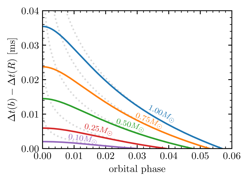
Figure 8: Time delay as a function of orbital phase for a system consisting of a Roche-lobe-overflowing donor star eclipsing a $1.4M_{\odot}$ NS companion. The donor is initially a $1\,M_{\odot}$ star at solar metallicity in a binary with an initial orbital period of $2$ days. Each solid line corresponds to a different point in time as mass transfer reduces the mass of the donor star to the value appearing in the caption, and shows the expected time delay from geometric optics for an edge-on system. Dotted lines indicate the expected time delay for the case of a point mass rather than a donor star model with an extended mass distribution.

IV.1 Number of eclipsed accreting neutron star binaries

We estimate the number of rapidly rotating NSs that are eclipsed either by a binary companion or the Sun through a population synthesis of NS binaries using the binary population synthesis code COSMIC Breivik et al. (2019). COSMIC evolves binary systems with a modified version of the binary evolution code BSE Hurley et al. (2002). The modified version includes updates to account for metallicity dependent winds Vink et al. (2001); Vink and de Koter (2005), neutrino driven core collapse supernova explosions Fryer et al. (2012), and compact object natal kicks Hobbs et al. (2005). We treat the star formation history (SFH) for the Milky Way Thin Disk, Thick Disk, and Bulge populations separately as outlined in Table 2. All binaries are initialized according to the observationally derived correlated joint probability distribution of Moe and Di Stefano (2017) over the primary mass, secondary mass, orbital period, eccentricity, and multiplicity of each binary. We assume all systems with a multiplicity greater than one are binary systems, thus ignoring triples and higher multiplicity systems.

Table 2: Star formation history (SFH) for Galactic components following McMillan (2011).

Component	Age [Gyr]	SFH	$Z$ [$Z_{\odot}$]	Mass [$M_{\odot}$]
Thin Disk	$10$	constant	1	$4.32\times 10^{10}$
Thick Disk	$11$	$1\,\rm{Gyr}$ burst	0.15	$1.44\times 10^{10}$
Bulge	$10$	$1\,\rm{Gyr}$ burst	$1$	$8.9\times 10^{9}$

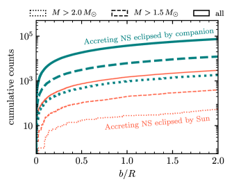
Figure 9: Cumulative counts of impact parameters below the abscissa value for the population of Galactic accreting NS binaries eclipsed by a companion (green, in units of donor Roche lobe radius) or the Sun (orange, in solar radii). Line styles indicate cuts on the donor mass.

We simulate all binaries from the zero-age main sequence and restrict our attention to the population containing a NS that is accreting from a stellar donor with $M_{\rm{D}}>0.05~{}\rm{M_{\odot}}$ at present. This criterion removes NSs that would experience time delays on the order of a microsecond or less when eclipsed by their companions; black widow pulsars, which are observed to eclipse, fall into this category Fruchter et al. (1988); Lyne et al. (1990); Freire (2005); Polzin et al. (2018); Guillemot et al. (2019) and so produce sub-microsecond time delays. We confirm that the present day orbital parameters are well sampled by increasing the number of simulated systems until the binary parameter distributions do not depend on the sample size, as described in Breivik et al. (2019).

We generate $500$ simulated Milky Way populations by re-sampling the simulated population with replacement. The number of accreting NS binaries in each Galactic component population is found by multiplying the number of simulated binaries by the ratio of the Galactic component mass to the total mass required to generate the simulated accreting NS population. Every re-sampled binary is assigned a position based on its Galactic component distribution following McMillan (2011) and a random inclination $i$ that is uniform in $\cos{i}$.

The statistics from 500 Milky Way populations are summarized in Table 3. To check the validity of our Milky Way population model, we compare to previous population synthesis studies. For our Thin Disk population, we first consider Nelemans et al. (2001), which finds a total population of $2.2\times 10^{6}$ NS–white dwarf binaries from a Thin Disk population with total mass $\sim 6\times 10^{10}\,M_{\odot}$ formed at an exponentially decreasing star formation rate. We find a total population $5.9\times 10^{6}$ NS-white dwarf binaries, without constraints on the donor mass or Roche lobe filling factor. Our yield is a factor of $\sim 4$ greater than Nelemans et al. (2001) if we take into account our lower Thin Disk mass of $4.32\times 10^{10}\,M_{\odot}$. For the Bulge population, we compare to van Haaften et al. (2015), which simulated the population of low mass X-ray binaries (LMXBs) with NS accretors in the Bulge and predict a population of $\sim 2.1\times 10^{3}$ NS LMXBs for a total Bulge mass of $1\times 10^{10}\,M_{\odot}$. Our model roughly agrees with van Haaften et al. (2015), though we predict a twice greater yield of NS LMXBs once we account for our relatively lower Bulge mass of $8.9\times 10^{9}\,M_{\odot}$. Direct comparisons between population synthesis studies which use different codes is difficult, thus rate differences within an order of magnitude are commonly accepted Toonen et al. (2014). Scaling our populations numbers down to match the numbers reported by Nelemans et al. (2001) and van Haaften et al. (2015), does not change our general conclusions.

Table 3: Accreting NS population statistics for the Galaxy. Here $N_{\mathrm{MW}}$ denotes the total number of accreting NSs expected in the galaxy with donors $>0.05M_{\odot}$, $N_{\mathrm{Donor,ecl}}$ is the number of those that are eclipsed by their companions, and $N_{{\odot,\mathrm{ecl}}}$ is the number of those expected to be eclipsed by the Sun.

Component	$N_{\mathrm{MW}}$	$N_{\mathrm{{Donor,ecl}}}$	$N_{{\odot,\mathrm{ecl}}}$
Thin Disk	$109,000$	$36,000\pm 160$	$1500\pm 40$
Thick Disk	$1700$	$450\pm 20$	$20\pm 5$
Bulge	$3400$	$920\pm 30$	$30\pm 5$

For each accreting NS we consider eclipses both by the donor companion and by the Sun. The impact parameter for the eclipse is

$$\frac{b}{R}=\frac{a}{R}\,\sin\left(\frac{\pi}{2}-i\right),$$ (23)

where for donor eclipses $a$ is the binary semimajor axis, $R$ is the donor Roche lobe radius, and $i$ is the binary inclination; for solar eclipses $a$ is an astronomical unit, $R$ is $R_{\odot}$ and $\pi/2-i$ is the ecliptic latitude.

Figure 9 shows the cumulative counts of impact parameters smaller than a given value for the populations of accreting NSs eclipsed by their donors (green) and by the Sun (orange) for a single Milky Way population. The different line styles show the fractions of the population which satisfy donor mass cuts of $M>2.0\,M_{\odot}$ and $M>1.5\,M_{\odot}$. As expected from Fig. 1, we find nearly two orders of magnitude fewer solar eclipses than donor eclipses for our accreting NS population. We find a slight excess in the fraction of solar eclipses when compared with the probability in Fig. 1 because NS accretors are highly concentrated in the Galactic plane, which intersects with the ecliptic plane.

V Detectability

We consider in turn all three effects caused by an eclipse: magnification $\Delta h/h\equiv 1-h^{\prime}/h$, deflection in the apparent sky location due to lensing $\Delta\theta$, and the variation in the Shapiro time delay $\Delta t_{s}\equiv\Delta t(b)-\Delta t(R_{\odot})$, as described in Eq. (5), Eq. (3), and Eq. (17), respectively. As shown in Section III, the characteristic magnitude of these effects for sources eclipsed by the Sun is

$$\frac{\Delta h}{h} \sim 0.01\,;$$ (24)

$$\Delta\theta \sim 1^{\prime\prime}\,;$$ (25)

$$\Delta t_{s} \sim 0.01~{}\mathrm{ms}\,.$$ (26)

As discussed in Section IV, in the case of a NS emitting GWs that is eclipsed by a binary companion, both the amplification and deflection are negligible, but the Shapiro time delay has a comparable magnitude as long as the mass of the companion star is comparable to that of the Sun.

Since the eclipse occupies only a small fraction of the overall observation, the measurement uncertainties from comparing the amplitude, location, and timing of the signal during the eclipse against the non-eclipse values are dominated by the uncertainties during the eclipse. Let $\rho$ be the total signal-to-noise ratio (SNR) over the full observation, and $\rho_{\mathrm{ec}}$ the SNR during the eclipse. We assume that the SNR is proportional to the square root of the duration of the observation Jaranowski et al. (1998). The scaling is weaker for initial detectability with a semi-coherent search Wette (2012), but we can assume that the source has already been detected, since that requires a much lower SNR than is necessary for measuring the eclipse properties, and a fully coherent analysis is used for parameter estimation. For example, for eclipses by the Sun, $\rho_{\mathrm{ec}}\approx\rho(R_{\odot}/(\pi~{}\mathrm{au}))^{1/2}\approx\rho(12~{}\mathrm{hr}/\mathrm{yr})^{1/2}\approx 0.04\rho$. The SNR required for measuring the variation of the different effects over the course of an eclipse can be estimated by dividing the observation into shorter segments. For example, one-hour observations would have individual SNRs of $\sim\rho(1~{}\mathrm{hr}/\mathrm{yr})^{1/2}\approx 0.01\rho$.

The measurement precision the GW signal amplitude, sky location, and timing during the eclipse are (e.g., Poisson and Will (1995); Krishnan et al. (2004); Fairhurst (2009); Mandel et al. (2018))

$$\frac{\delta h}{h} \sim \frac{1}{\rho_{\mathrm{ec}}}\,;$$ (27)

$$\delta\theta \sim \frac{1}{\rho_{\mathrm{ec}}}\frac{c\tau_{\mathrm{GW}}}{v_{\oplus}\tau_{\mathrm{ec}}}\simeq\frac{600^{\prime\prime}}{\rho_{\rm ec}}\left(\frac{1000~{}\mathrm{Hz}}{f_{\rm GW}}\right)\left(\frac{1~{}\mathrm{hr}}{\tau_{\rm ec}}\right)\,;\quad$$ (28)

$$\delta t \sim \frac{\tau_{\mathrm{GW}}}{\rho_{\mathrm{ec}}}=\frac{1~{}\mathrm{ms}}{\rho_{\rm ec}}\left(\frac{1000~{}\mathrm{Hz}}{f_{\rm GW}}\right)\,,$$ (29)

where $\tau_{\mathrm{GW}}=1/f_{\mathrm{GW}}$ is the GW period, $\tau_{\mathrm{ec}}$ is the duration of the observation, and $v_{\oplus}=2\pi~{}\mathrm{au\,yr^{-1}}$ is the orbital speed of the Earth. This allows us to compute the detectability of these quantities:

$$\frac{\Delta h}{\delta h} \sim 0.01\rho_{\mathrm{ec}}\,;$$ (30)

$$\frac{\Delta\theta}{\delta\theta} \sim 0.002\rho_{\mathrm{ec}}\left(\frac{f_{\rm GW}}{1000~{}\mathrm{Hz}}\right)\left(\frac{\tau_{\rm ec}}{1~{}\mathrm{hr}}\right)\,;$$ (31)

$$\frac{\Delta t}{\delta t} \sim 0.01\rho_{\mathrm{ec}}\left(\frac{f_{\rm GW}}{1000~{}\mathrm{Hz}}\right)\,.$$ (32)

As can be seen, for very high-frequency signals with $f_{\rm GW}\sim 10^{3}~{}\mathrm{Hz}$ and a time of observation of $\sim 1~{}\mathrm{hr}$ the detectability of the three effects are comparable in this order-of-magnitude analysis.

In order to make a useful measurement, a quantity such as $\Delta t/\delta t$ should at the least exceed $1$. This corresponds to the requirement $\rho_{\mathrm{ec}}>100$ for a signal with a GW frequency of $\sim 1000~{}\mathrm{Hz}$. For eclipses by the Sun, this means that the full SNR must be $\rho>2500$; for eclipses by the AMXP’s companion lasting $10\%$ of the orbit, the requirement is a more modest $\rho>300$. The SNR is expected to improve by a factor of $\sim 30$ – $50$ at high frequencies between the Advanced LIGO second observing run sensitivity – the latest data for which continuous-wave upper limits are available Abbott and et al. (2019c) – and next-generation detectors such as the Einstein Telescope Hild et al. (2011) and the Cosmic Explorer Abbott et al. (2017d). Moreover, since semi-coherent searches with segments of length $T_{\mathrm{seg}}$ between half an hour and of order of one week were typically used in the past Abbott and et al. (2019c), the optimal coherent SNR would naturally be a factor of $(\mathrm{yr}/T_{\mathrm{seg}})^{1/4}\approx 3$ to $10$ times greater. Thus, if there are favourably located sources at high frequencies just below the latest upper limits (corresponding to $\rho\gtrsim 10$, which would be translated to $\rho\gtrsim 1000$ with an optimal coherent analysis of next-generation data), it should be possible to observe eclipse signatures with next-generation detectors.

VI Conclusions

We demonstrated how the observation of an eclipsing GW source provides unique information on the mass distribution of the eclipsing object, and showed that CWs with frequencies $>100~{}\mathrm{Hz}$ are best suited for this purpose. For the case of a source eclipsed by the Sun, a GW signal would experience an apparent change in source position of a few arcseconds, a change in strain amplitude by up to $\sim 4\%$ and a Shapiro time delay of up to $\sim 0.034~{}\mathrm{ms}$. An even more likely possibility is that a source of GWs is eclipsed by a binary companion, in which case the only signature of the eclipse for an observer on Earth would be a variable time delay of a magnitude similar to that produced by the Sun.

The potential to observe lensing of CW sources depends upon the currently unknown amplitude of their GW emission. No CW sources have yet been detected. The effects of eclipses on the signal are small. Moreover, the SNR accumulated during the eclipse is a factor of $\sim 3$ to $\sim 25$ smaller than the total SNR. Therefore, eclipse lensing may be safely neglected for observations with current-generation detectors. However, if CW sources are just at the limit of the sensitivity of early current-generation detectors Abbott et al. (2019c), eclipses could potentially be observed by next-generation detectors.

To obtain interesting constraints on the mass distribution of the eclipsing object will require SNRs of order of $10^{3}$. Such large SNRs may motivate the development of specialised detectors. Since a much larger SNR is required to measure the stellar interior than to detect a signal, we will know ahead of time the frequency of interest. This makes eclipsing CW sources an attractive target for tuneable narrow-band detectors. These can achieve enhanced sensitivity in a small range of frequencies compared to wide-band detectors. Tuneable detectors have been suggested for observations of binary neutron star coalescences, where they can track the inspiral and observe the post-merger signal Simakov (2014); Hughes (2002); Graham et al. (2016), or to increase detection prospects for supernovae Srivastava et al. (2019). In comparison, eclipsing CW sources are a far simpler target, since detectors only need to focus on a single known frequency. Additionally, the timing of eclipses by the Sun can be predicted years in advance, so tuning does not need to be done dynamically, but can follow a well-planned schedule. Observations from multiple eclipsing sources could be combined to give a more detailed map of the Sun’s interior.

While eclipsing CWs provide a new probe of stellar interiors, we have not addressed the measurement precision necessary to provide meaningful constraints on stellar structure. For the Sun, helioseismology and neutrino detections already provide stringent constraints (cf. Christensen-Dalsgaard (2018)). In this context, unless extremely bright high-frequency sources of CWs are detected, even next-generation detectors might not be sufficient to improve upon the known constraints on the structure of the Sun. Still, additional work is required to properly quantify by how much our lensing predictions are modified by uncertainties in solar structure. For the case when the eclipsing star is a binary companion to a GW source, neutrinos are undetectable, and asteroseismic measurements cannot be performed to the same precision as for the Sun. In this case, the measurement of eclipses of GW sources could provide a unique view into their stellar interiors. Despite its complexity, the detection of eclipses would provide an unbiased measurement of the mass distribution of a star, independent of uncertainties such as the composition or nuclear reaction rates.

Appendix A Wave optics calculations

A.1 The Kirchhoff integral

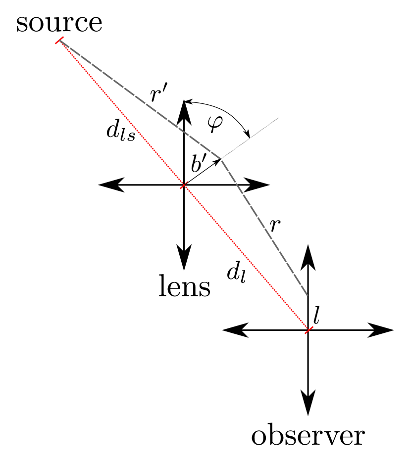
Figure 10: Variables used for the computation of the Kirchhoff integral, in order to compute the effect of the Sun on GWs without the use of geometric optics. $r$ is the distance between the observer and a point in the plane of the lens, while $r^{\prime}$ is the distance between the source and the same point. The distance $l$ corresponds to the separation between the observer and the optical axis, which is the line that joins the source and the lens. The lines of length $r$ and $r^{\prime}$ are not necessarily coplanar, and are not meant to represent an actual trajectory (within the geometric optics approximation) from the source to the observer.

Following the work of Ohanian (1974); Bontz and Haugan (1981), if the amplitude $\Psi$ of a wave is known at a surface $S$ surrounding the observer and inside which the wave propagates freely, its amplitude at the observer can be computed using the Kirchhoff integral,

$$\Psi_{o}=\frac{1}{4\pi}\int_{S}\left(\left[\nabla\Psi\right]\frac{e^{ikr}}{r}-\Psi\nabla\left[\frac{e^{ikr}}{r}\right]\right)\cdot\mathrm{d}\vec{A},$$ (33)

where $k\equiv 2\pi/\lambda$ is the wavenumber and $r$ is the distance between the observer and a point at the surface $S$. For the particular case under consideration, the surface of integration can be taken to be the plane of the lens (see Fig. 10). The effect of the lens can be accounted for as a phase shift due to the time delay for a given impact parameter $b$,

$$\Psi(b)=\frac{A_{0}}{r^{\prime}}e^{i(kr^{\prime}-\omega\Delta t(b))},$$ (34)

where $\omega=2\pi f_{\rm GW}$ is the angular frequency of the wave, $r^{\prime}$ is the distance between the source and a point in the plane of the lens, and $A_{0}$ is a constant that sets the intensity of the wave. To compute the Kirchhoff integral we only consider the case of sources eclipsed by the sun and observed from Earth, in which case $b^{\prime}$ can be approximated as $b$ (see Fig. 4). Here we ignore the phase shift $\omega t$ for the time evolution of the wave, as this factors out in the calculation of time delays and amplitude changes. Assuming $k\ll d_{l}^{-1}$ and $k\ll d_{ls}^{-1}$, combining Eq. (33) and Eq. (34) results in

$$\Psi_{o}(l) = -\frac{ikA_{0}}{4\pi}\int_{0}^{\infty}\int_{0}^{2\pi}e^{i(kr+kr^{\prime}-\omega\Delta t(b))}\qquad\qquad$$ (35)

$$\times\frac{1}{rr^{\prime}}\left(\frac{d_{l}}{r}+\frac{d_{ls}}{r^{\prime}}\right)b\,\mathrm{d}\varphi\,\mathrm{d}b,$$

where

$$r = \sqrt{d_{l}^{2}+(l-b\cos\varphi)^{2}+b^{2}\sin^{2}\varphi},$$ (36)

$$r^{\prime} = \sqrt{d_{ls}^{2}+b^{2}},$$ (37)

$l$ is the distance of the observer from the optical axis while $\varphi$ is an angle in the optical plane (see Fig. 10). Given $\Psi_{o}(l)$, the amplification of a GW arriving at Earth is given by the ratio of $\Psi_{o}(l)$ to the expected amplitude in the absence of a lens,

$$\frac{h^{\prime}(b)}{h}=\frac{|\Psi_{o}|(d_{l}+d_{ls})}{A_{0}},$$ (38)

while the time delay can be computed by comparing the phase of the wave at different values of $l$,

$$\omega|\Delta t_{s}|=\arccos\left[\frac{\Psi_{o}(b)\cdot\Psi_{o}(R_{\odot})}{|\Psi_{o}(b)||\Psi_{o}(R_{\odot})|}\right],$$ (39)

where $\Psi_{o}(b)\cdot\Psi_{o}(R_{\odot})$ denotes the complex dot product of $\Psi_{o}(b)$ and $\Psi_{o}(R_{\odot})$.

The computation of Eq. (36) can be simplified in the limit $l\ll d_{l}$, in which case

$$r = r_{0}\left[1+\frac{bl\cos\varphi}{r_{0}^{2}}-\mathcal{O}\left(\frac{b^{2}l^{2}}{r_{0}^{4}}\right)\right],$$ (40)

where $r_{0}=\sqrt{d_{l}^{2}+b^{2}+l^{2}}$. For the terms outside the exponential factor in Eq. (35) one can simply approximate $r\simeq r_{0}$, but the term of order $\mathcal{O}(bl/r_{0}^{2})$ in Equation (40) needs to be included in the exponential to prevent errors in the phase larger than those induced by the lens. Under these approximations one has that

$$\Psi_{o}(l) = -\frac{ikA_{0}}{4\pi}\int_{0}^{\infty}\int_{0}^{2\pi}e^{i(kr_{0}+kr^{\prime}+kbl\cos\varphi/r_{0}-\omega\Delta t(b))}$$ (41)

$$\times\frac{1}{r_{0}r^{\prime}}\left(\frac{d_{l}}{r_{0}}+\frac{d_{ls}}{r^{\prime}}\right)b\,\mathrm{d}\varphi\,\mathrm{d}b,$$

and the integral over $\phi$ can be computed analytically resulting in

$$\Psi_{o}(l) = -\frac{ikA_{0}}{2}\int_{0}^{\infty}e^{i(kr_{0}+kr^{\prime}-\omega\Delta t(b))}\qquad\qquad$$ (42)

$$\times\frac{J_{0}(kbl/r_{0})}{r_{0}r^{\prime}}\left(\frac{d_{l}}{r_{0}}+\frac{d_{ls}}{r^{\prime}}\right)b\,\mathrm{d}b,$$

where $J_{0}$ is the Bessel function of the first kind and order zero.

Previous work on the impact of the Sun on GWs Ohanian (1974); Bontz and Haugan (1981) dealt with the change in amplitude of the wave near the caustics of the solar lens (regions where multiple images are formed). In this case the integral in Eq. (42) is dominated by points around the value of $b$ for which geometrical optics predicts rays converge at a distance $d_{l}$ from the optical plane. This allows an analytical approximation of the result using the stationary phase approximation Born and Wolf (1999) and leads to the conclusion of Ohanian (1974) that no significant amplification occurs for frequencies $f_{\rm GW}<10^{4}$ Hz. The situation is different for an observer at Earth as the Earth is not located at a caustic of the Sun, requiring the calculation of the Kirchhoff integral in the entire lens plane; from our solar model we predict caustics occur at a distance of $\gtrsim 20~{}\mathrm{au}$ from the Sun.

A.2 Numerical integration of the Kirchhoff integral

Numerically computing the integral in Eq. (42) is difficult, as both the exponential term and the Bessel function change sign leading to a rapidly oscillating integrand. For $b\gg d_{0}$ we have that $r_{0}\sim b$, such that the argument of the Bessel function becomes constant and only the rapid oscillation of the exponential factor remains problematic. To remedy this, we make the following change of variables:

$$y = r_{0}+r^{\prime}-d_{ls}-\sqrt{d_{l}^{2}+l^{2}},$$ (43)

$$\mathrm{d}y = \left(\frac{1}{r_{0}}+\frac{1}{r^{\prime}}\right)b\,\mathrm{d}b,$$ (44)

which, except for the time delay produced by the lens, leaves the argument of the complex exponential in Eq. (42) as the integration variable. Ignoring constant phase shifts the wave amplitude is then

$$\Psi_{o}(l) = -\frac{kA_{0}e^{ik\sqrt{d_{l}^{2}+l^{2}}}}{2}\int_{0}^{\infty}e^{i(ky-\omega\Delta t(b))}\qquad\qquad$$ (45)

$$\times\frac{J_{0}(kbl/r_{0})}{r_{0}+r^{\prime}}\left(\frac{d_{l}}{r_{0}}+\frac{d_{ls}}{r^{\prime}}\right)\mathrm{d}y.$$

We can then perform the integrand over each individual cycle produced by the term $ky$ in the complex exponential, defining for an integer value $j$ the quantity

$$A_{j} = -\frac{kA_{0}}{2}\int_{2\pi j/k}^{2\pi(j+1)/k}e^{i(ky-\omega\Delta t(b))}\qquad\qquad$$ (46)

$$\times\frac{J_{0}(kbl/r_{0})}{r_{0}+r^{\prime}}\left(\frac{d_{l}}{r_{0}}+\frac{d_{ls}}{r^{\prime}}\right)\mathrm{d}y,$$

such that

$$\Psi_{o}(l)=e^{ik\sqrt{d_{l}^{2}+l^{2}}}\sum_{j=0}^{\infty}A_{j}.$$ (47)

If there exists an $N$ such that the value of $A_{j}$ changes slowly with $j$ for $j>N$, then it is useful to separate the sum to include all terms up to $N$, and express the rest as an integral,

$$\sum_{j=0}^{\infty}A_{j} = \sum_{j=0}^{N}A_{j}+\int_{N+1}^{\infty}A(x)\,\mathrm{d}x$$ (48)

where $A(x)$ is a function that is equal to $A_{j}$ with $j={\rm floor}(x)$ being the nearest integer to $x$ that is smaller than $x$. Switching variables to $z=\ln x$ in the integral results in

$$\sum_{j=0}^{\infty}A_{j} = \sum_{j=0}^{N}A_{j}+\int_{\ln(N+1)}^{\infty}\frac{A(e^{z})}{e^{z}}\,\mathrm{d}z.$$ (49)

Since $A_{j}$ varies slowly for $j>N$, the integral can be estimated by adding over logarithmic intervals $\Delta z$,

$$\sum_{j=0}^{\infty}A_{j} \simeq \sum_{j=0}^{N}A_{j}+\sum_{m=0}^{\infty}\frac{A(e^{\ln(N+1)+m\Delta z})}{e^{\ln(N+1)+m\Delta z}}\Delta z.$$ (50)

This allows the calculation of the integral up to a large number of cycles, without individually computing the contribution of each one. Using this, we numerically compute the real and imaginary part of $\Psi_{0}(l)$. In addition, when evaluating cosines or sines in Eq. (46), rather than computing, for example, $\cos(ky-\omega\Delta t)$ we compute instead $\cos[k(y-2\pi j/k)-\omega\Delta t]$. This prevents the evaluation of trigonometric functions with large arguments and reduces numerical errors.

Figure 11 shows an example of this integration, showing only the imaginary part of $\Psi_{o}$ as the number of cycles $n$ included in the calculation of the integral is increased. In this particular example the integral is directly computed up to $N=10^{6}$, and then estimated up to $10^{15}$ cycles using $10^{6}$ equally spaced logarithmic intervals. As it can be seen, the integral converges after $10^{10}$ cycles. Directly computing the integral up to that point is extremely expensive, which is the reason why we require the approximation discussed in this Appendix. Evaluating Eq. (46) still requires a choice for $d_{ls}$ and $d_{l}$. The calculations shown in Section III.3 were done using a distance between the lens and the source of $d_{ls}=1\;\mathrm{pc}$, but we have verified that the resulting amplification and time delays are equivalent if the integrations are done using $d_{ls}=0.1\;\mathrm{pc}$.

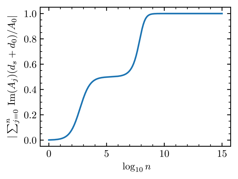
Figure 11: Computation of the imaginary part of $\sum A_{j}$ for $l=0.05R_{\odot}$, considering a $100$ Hz source located at $1$ parsec and observed at $1$ au from the Sun. The ordinate-axis is normalized to the expected intensity of the wave in the absence of a lens. The abscissa-axis represents the number of cycles added (see Appendix A).

References

- Weber (1969) J. Weber, Physical Review Letters 22, 1320 (1969).
- Lawrence (1971) J. K. Lawrence, Nuovo Cimento B Serie 6, 225 (1971).
- Ohanian (1973) H. C. Ohanian, Phys. Rev. D 8, 2734 (1973).
- Bontz and Haugan (1981) R. J. Bontz and M. P. Haugan, Ap&SS 78, 199 (1981).
- Ohanian (1983) H. C. Ohanian, Astrophys. J. 271, 551 (1983).
- Kokkotas (2008) K. D. Kokkotas, Reviews in Modern Astronomy 20, 140 (2008), arXiv:0809.1602 [astro-ph] .
- Smith et al. (2018) G. P. Smith, M. Jauzac, J. Veitch, W. M. Farr, R. Massey, and J. Richard, MNRAS 475, 3823 (2018), arXiv:1707.03412 [astro-ph.HE] .
- Ng et al. (2018) K. K. Y. Ng, K. W. K. Wong, T. Broadhurst, and T. G. F. Li, Phys. Rev. D 97, 023012 (2018), arXiv:1703.06319 [astro-ph.CO] .
- Li et al. (2018) S.-S. Li, S. Mao, Y. Zhao, and Y. Lu, MNRAS 476, 2220 (2018), arXiv:1802.05089 [astro-ph.CO] .
- Hannuksela et al. (2019) O. A. Hannuksela, K. Haris, K. K. Y. Ng, S. Kumar, A. K. Mehta, D. Keitel, T. G. F. Li, and P. Ajith, ApJ 874, L2 (2019), arXiv:1901.02674 [gr-qc] .
- Takahashi and Nakamura (2003) R. Takahashi and T. Nakamura, Astrophys. J. 595, 1039 (2003), astro-ph/0305055 .
- Moylan et al. (2008) A. J. Moylan, D. E. McClelland, S. M. Scott, A. C. Searle, and G. V. Bicknell, in The Eleventh Marcel Grossmann Meeting On Recent Developments in Theoretical and Experimental General Relativity, Gravitation and Relativistic Field Theories (2008) pp. 807–823, arXiv:0710.3140 [gr-qc] .
- Liao et al. (2019) K. Liao, M. Biesiada, and X.-L. Fan, Astrophys. J. 875, 139 (2019), arXiv:1903.06612 [gr-qc] .
- Abbott et al. (2016) B. P. Abbott, R. Abbott, T. D. Abbott, M. R. Abernathy, F. Acernese, K. Ackley, C. Adams, T. Adams, P. Addesso, R. X. Adhikari, and et al., Physical Review Letters 116, 061102 (2016), arXiv:1602.03837 [gr-qc] .
- Abbott et al. (2019a) B. P. Abbott, R. Abbott, T. D. Abbott, S. Abraham, F. Acernese, K. Ackley, C. Adams, R. X. Adhikari, and et al., Physical Review X 9, 031040 (2019a), arXiv:1811.12907 [astro-ph.HE] .
- Abbott et al. (2017a) B. P. Abbott, R. Abbott, T. D. Abbott, F. Acernese, K. Ackley, C. Adams, T. Adams, P. Addesso, R. X. Adhikari, V. B. Adya, and et al., Physical Review Letters 119, 161101 (2017a), arXiv:1710.05832 [gr-qc] .
- Aasi et al. (2015) J. Aasi, B. P. Abbott, R. Abbott, T. Abbott, M. R. Abernathy, K. Ackley, C. Adams, T. Adams, et al., Classical and Quantum Gravity 32, 074001 (2015), arXiv:1411.4547 [gr-qc] .
- Acernese et al. (2015) F. Acernese, M. Agathos, K. Agatsuma, D. Aisa, N. Allemandou, A. Allocca, J. Amarni, P. Astone, et al., Classical and Quantum Gravity 32, 024001 (2015), arXiv:1408.3978 [gr-qc] .
- Cyranski and Lubkin (1974) J. F. Cyranski and E. Lubkin, Annals of Physics 87, 205 (1974).
- Note (1) doi.org/10.5281/zenodo.2653899.
- Amaro-Seoane et al. (2017) P. Amaro-Seoane, H. Audley, S. Babak, J. Baker, E. Barausse, P. Bender, E. Berti, P. Binetruy, et al., arXiv e-prints (2017), arXiv:1702.00786 [astro-ph.IM] .
- Stroeer and Vecchio (2006) A. Stroeer and A. Vecchio, Classical and Quantum Gravity 23, S809 (2006), astro-ph/0605227 .
- Kupfer et al. (2018) T. Kupfer, V. Korol, S. Shah, G. Nelemans, T. R. Marsh, G. Ramsay, P. J. Groot, D. T. H. Steeghs, and E. M. Rossi, MNRAS 480, 302 (2018), arXiv:1805.00482 [astro-ph.SR] .
- Prix (2009) R. Prix, Astrophys. Space Sci. Lib. 357, 651 (2009).
- Riles (2017) K. Riles, Modern Physics Letters A 32, 1730035-685 (2017), arXiv:1712.05897 [gr-qc] .
- Zimmermann and Szedenits (1979) M. Zimmermann and E. Szedenits, Jr., Phys. Rev. D 20, 351 (1979).
- Abbott and et al. (2019a) B. P. Abbott and et al., Astrophys. J. 879, 10 (2019a), arXiv:1902.08507 [astro-ph.HE] .
- Abbott and et al. (2019b) B. P. Abbott and et al., Phys. Rev. D 99, 122002 (2019b), arXiv:1902.08442 [gr-qc] .
- Abbott and et al. (2019c) B. P. Abbott and et al., Phys. Rev. D 100, 024004 (2019c), arXiv:1903.01901 [astro-ph.HE] .
- Wagoner (1984) R. V. Wagoner, Astrophys. J. 278, 345 (1984).
- Bildsten (1998) L. Bildsten, ApJ 501, L89 (1998), astro-ph/9804325 .
- Haskell (2015) B. Haskell, International Journal of Modern Physics E 24, 1541007 (2015), arXiv:1509.04370 [astro-ph.HE] .
- Markwardt and Strohmayer (2010) C. B. Markwardt and T. E. Strohmayer, ApJ 717, L149 (2010), arXiv:1005.3479 [astro-ph.HE] .
- Reardon et al. (2016) D. J. Reardon, G. Hobbs, W. Coles, Y. Levin, M. J. Keith, M. Bailes, N. D. R. Bhat, S. Burke-Spolaor, S. Dai, M. Kerr, P. D. Lasky, R. N. Manchester, S. Osłowski, V. Ravi, R. M. Shannon, W. van Straten, L. Toomey, J. Wang, L. Wen, X. P. You, and X.-J. Zhu, MNRAS 455, 1751 (2016), arXiv:1510.04434 [astro-ph.HE] .
- Ray et al. (2012) P. S. Ray, A. A. Abdo, D. Parent, D. Bhattacharya, B. Bhattacharyya, F. Camilo, I. Cognard, G. Theureau, E. C. Ferrara, A. K. Harding, D. J. Thompson, P. C. C. Freire, L. Guillemot, Y. Gupta, J. Roy, J. W. T. Hessels, S. Johnston, M. Keith, R. Shannon, M. Kerr, P. F. Michelson, R. W. Romani, M. Kramer, M. A. McLaughlin, S. M. Ransom, M. S. E. Roberts, P. M. Saz Parkinson, M. Ziegler, D. A. Smith, B. W. Stappers, P. Weltevrede, and K. S. Wood, arXiv e-prints (2012), arXiv:1205.3089 [astro-ph.HE] .
- Lyne et al. (2015) A. G. Lyne, C. A. Jordan, F. Graham-Smith, C. M. Espinoza, B. W. Stappers, and P. Weltevrede, MNRAS 446, 857 (2015), arXiv:1410.0886 [astro-ph.HE] .
- Bradshaw et al. (1999) C. F. Bradshaw, E. B. Fomalont, and B. J. Geldzahler, ApJ 512, L121 (1999).
- Markwardt et al. (2002) C. B. Markwardt, J. H. Swank, T. E. Strohmayer, J. J. M. in ’t Zand, and F. E. Marshall, ApJ 575, L21 (2002), astro-ph/0206491 .
- Ferrigno et al. (2011) C. Ferrigno, E. Bozzo, M. Falanga, L. Stella, S. Campana, T. Belloni, G. L. Israel, L. Pavan, E. Kuulkers, and A. Papitto, A&A 525, A48 (2011), arXiv:1005.4554 [astro-ph.HE] .
- Manchester et al. (2005) R. N. Manchester, G. B. Hobbs, A. Teoh, and M. Hobbs, AJ 129, 1993 (2005), astro-ph/0412641 .
- Manchester (2004) R. N. Manchester, Science 304, 542 (2004).
- Shapiro (1964) I. I. Shapiro, Physical Review Letters 13, 789 (1964).
- Aasi et al. (2014) J. Aasi, J. Abadie, B. P. Abbott, R. Abbott, T. Abbott, M. R. Abernathy, T. Accadia, F. Acernese, C. Adams, T. Adams, and et al., Astrophys. J. 785, 119 (2014), arXiv:1309.4027 [astro-ph.HE] .
- Espinoza et al. (2011) C. M. Espinoza, A. G. Lyne, B. W. Stappers, and M. Kramer, MNRAS 414, 1679 (2011), arXiv:1102.1743 [astro-ph.HE] .
- Abbott et al. (2017b) B. P. Abbott, R. Abbott, T. D. Abbott, F. Acernese, K. Ackley, C. Adams, T. Adams, P. Addesso, et al., Phys. Rev. D 95, 122003 (2017b), arXiv:1704.03719 [gr-qc] .
- Abbott et al. (2017c) B. P. Abbott, R. Abbott, T. D. Abbott, F. Acernese, K. Ackley, C. Adams, T. Adams, P. Addesso, et al., Astrophys. J. 847, 47 (2017c), arXiv:1706.03119 [astro-ph.HE] .
- Abbott et al. (2019b) B. P. Abbott, R. Abbott, T. D. Abbott, S. Abraham, F. Acernese, K. Ackley, C. Adams, R. X. Adhikari, et al., arXiv e-prints (2019b), arXiv:1906.12040 [gr-qc] .
- Meadors et al. (2017) G. D. Meadors, E. Goetz, K. Riles, T. Creighton, and F. Robinet, Phys. Rev. D 95, 042005 (2017), arXiv:1610.09391 [gr-qc] .
- Patruno and Watts (2012) A. Patruno and A. L. Watts, ArXiv e-prints (2012), arXiv:1206.2727 [astro-ph.HE] .
- Lasky (2015) P. D. Lasky, PASA 32, e034 (2015), arXiv:1508.06643 [astro-ph.HE] .
- Bahcall et al. (1995) J. N. Bahcall, M. H. Pinsonneault, and G. J. Wasserburg, Reviews of Modern Physics 67, 781 (1995), arXiv:hep-ph/9505425 [hep-ph] .
- Paxton et al. (2011) B. Paxton, L. Bildsten, A. Dotter, F. Herwig, P. Lesaffre, and F. Timmes, ApJS 192, 3 (2011), arXiv:1009.1622 [astro-ph.SR] .
- Paxton et al. (2013) B. Paxton, M. Cantiello, P. Arras, L. Bildsten, E. F. Brown, A. Dotter, C. Mankovich, M. H. Montgomery, D. Stello, F. X. Timmes, and R. Townsend, ApJS 208, 4 (2013), arXiv:1301.0319 [astro-ph.SR] .
- Paxton et al. (2015) B. Paxton, P. Marchant, J. Schwab, E. B. Bauer, L. Bildsten, M. Cantiello, L. Dessart, R. Farmer, H. Hu, N. Langer, R. H. D. Townsend, D. M. Townsley, and F. X. Timmes, ApJS 220, 15 (2015), arXiv:1506.03146 [astro-ph.SR] .
- Paxton et al. (2018) B. Paxton, J. Schwab, E. B. Bauer, L. Bildsten, S. Blinnikov, P. Duffell, R. Farmer, J. A. Goldberg, P. Marchant, E. Sorokina, A. Thoul, R. H. D. Townsend, and F. X. Timmes, ApJS 234, 34 (2018), arXiv:1710.08424 [astro-ph.SR] .
- Vinyoles et al. (2017) N. Vinyoles, A. M. Serenelli, F. L. Villante, S. Basu, J. Bergström, M. C. Gonzalez-Garcia, M. Maltoni, C. Peña-Garay, and N. Song, Astrophys. J. 835, 202 (2017), arXiv:1611.09867 [astro-ph.SR] .
- Clark (1972) E. E. Clark, MNRAS 158, 233 (1972).
- Refsdal (1964) S. Refsdal, MNRAS 128, 295 (1964).
- Backer and Hellings (1986) D. C. Backer and R. W. Hellings, ARA&A 24, 537 (1986).
- Richter and Matzner (1983) G. W. Richter and R. A. Matzner, Phys. Rev. D 28, 3007 (1983).
- Ohanian (1974) H. C. Ohanian, International Journal of Theoretical Physics 9, 425 (1974).
- Cook et al. (1994) G. B. Cook, S. L. Shapiro, and S. A. Teukolsky, Astrophys. J. 424, 823 (1994).
- Hessels et al. (2006) J. W. T. Hessels, S. M. Ransom, I. H. Stairs, P. C. C. Freire, V. M. Kaspi, and F. Camilo, Science 311, 1901 (2006), arXiv:astro-ph/0601337 [astro-ph] .
- Rappaport et al. (1983) S. Rappaport, F. Verbunt, and P. C. Joss, Astrophys. J. 275, 713 (1983).
- Breivik et al. (2019) K. Breivik, S. C. Coughlin, M. Zevin, C. L. Rodriguez, K. Kremer, C. S. Ye, J. J. Andrews, M. Kurkowski, M. C. Digman, S. L. Larson, and F. A. Raso, arXiv e-prints (2019), arXiv:1911.00903 [astro-ph.HE] .
- Hurley et al. (2002) J. R. Hurley, C. A. Tout, and O. R. Pols, MNRAS 329, 897 (2002), astro-ph/0201220 .
- Vink et al. (2001) J. S. Vink, A. de Koter, and H. J. G. L. M. Lamers, A&A 369, 574 (2001), astro-ph/0101509 .
- Vink and de Koter (2005) J. S. Vink and A. de Koter, A&A 442, 587 (2005), astro-ph/0507352 .
- Fryer et al. (2012) C. L. Fryer, K. Belczynski, G. Wiktorowicz, M. Dominik, V. Kalogera, and D. E. Holz, Astrophys. J. 749, 91 (2012), arXiv:1110.1726 [astro-ph.SR] .
- Hobbs et al. (2005) G. Hobbs, D. R. Lorimer, A. G. Lyne, and M. Kramer, MNRAS 360, 974 (2005), astro-ph/0504584 .
- Moe and Di Stefano (2017) M. Moe and R. Di Stefano, ApJS 230, 15 (2017), arXiv:1606.05347 [astro-ph.SR] .
- McMillan (2011) P. J. McMillan, MNRAS 414, 2446 (2011), arXiv:1102.4340 .
- Fruchter et al. (1988) A. S. Fruchter, D. R. Stinebring, and J. H. Taylor, Nature (London) 333, 237 (1988).
- Lyne et al. (1990) A. G. Lyne, R. N. Manchester, N. D’Amico, L. Staveley-Smith, S. Johnston, J. Lim, A. S. Fruchter, W. M. Goss, and D. Frail, Nature (London) 347, 650 (1990).
- Freire (2005) P. C. C. Freire, in Binary Radio Pulsars, Astronomical Society of the Pacific Conference Series, Vol. 328, edited by F. A. Rasio and I. H. Stairs (2005) p. 405, arXiv:astro-ph/0404105 [astro-ph] .
- Polzin et al. (2018) E. J. Polzin, R. P. Breton, A. O. Clarke, V. I. Kondratiev, B. W. Stappers, J. W. T. Hessels, C. G. Bassa, J. W. Broderick, J. M. Grießmeier, C. Sobey, S. ter Veen, J. van Leeuwen, and P. Weltevrede, MNRAS 476, 1968 (2018), arXiv:1802.02594 [astro-ph.HE] .
- Guillemot et al. (2019) L. Guillemot, F. Octau, I. Cognard, G. Desvignes, P. C. C. Freire, D. A. Smith, G. Theureau, and T. H. Burnett, A&A 629, A92 (2019), arXiv:1907.09778 [astro-ph.HE] .
- Nelemans et al. (2001) G. Nelemans, L. R. Yungelson, and S. F. Portegies Zwart, A&A 375, 890 (2001), astro-ph/0105221 .
- van Haaften et al. (2015) L. M. van Haaften, G. Nelemans, R. Voss, M. V. van der Sluys, and S. Toonen, A&A 579, A33 (2015), arXiv:1505.03629 [astro-ph.SR] .
- Toonen et al. (2014) S. Toonen, J. S. W. Claeys, N. Mennekens, and A. J. Ruiter, A&A 562, A14 (2014), arXiv:1311.6503 [astro-ph.SR] .
- Jaranowski et al. (1998) P. Jaranowski, A. Królak, and B. F. Schutz, Physical Review D 58, 063001 (1998), arXiv:gr-qc/9804014 [gr-qc] .
- Wette (2012) K. Wette, Physical Review D 85, 042003 (2012), arXiv:1111.5650 [gr-qc] .
- Poisson and Will (1995) E. Poisson and C. M. Will, Phys. Rev. D 52, 848 (1995), arXiv:gr-qc/9502040 .
- Krishnan et al. (2004) B. Krishnan, A. M. Sintes, M. A. Papa, B. F. Schutz, S. Frasca, and C. Palomba, Phys. Rev. D 70, 082001 (2004), arXiv:gr-qc/0407001 [gr-qc] .
- Fairhurst (2009) S. Fairhurst, New Journal of Physics 11, 123006 (2009).
- Mandel et al. (2018) I. Mandel, A. Sesana, and A. Vecchio, Classical and Quantum Gravity 35, 054004 (2018), arXiv:1710.11187 [astro-ph.HE] .
- Hild et al. (2011) S. Hild, M. Abernathy, F. Acernese, P. Amaro-Seoane, N. Andersson, K. Arun, F. Barone, B. Barr, et al., Classical and Quantum Gravity 28, 094013 (2011), arXiv:1012.0908 [gr-qc] .
- Abbott et al. (2017d) B. P. Abbott, R. Abbott, T. D. Abbott, M. R. Abernathy, K. Ackley, C. Adams, P. Addesso, R. X. Adhikari, V. B. Adya, C. Affeldt, et al., Classical and Quantum Gravity 34, 044001 (2017d), arXiv:1607.08697 [astro-ph.IM] .
- Abbott et al. (2019c) B. P. Abbott et al., arXiv e-prints (2019c), arXiv:1304.0670 [gr-qc] .
- Simakov (2014) D. A. Simakov, Phys. Rev. D 90, 102003 (2014), arXiv:1311.2766 [gr-qc] .
- Hughes (2002) S. A. Hughes, Phys. Rev. D 66, 102001 (2002), gr-qc/0209012 .
- Graham et al. (2016) P. W. Graham, J. M. Hogan, M. A. Kasevich, and S. Rajendran, Phys. Rev. D 94, 104022 (2016), arXiv:1606.01860 [physics.atom-ph] .
- Srivastava et al. (2019) V. Srivastava, S. Ballmer, D. A. Brown, C. Afle, A. Burrows, D. Radice, and D. Vartanyan, arXiv e-prints , arXiv:1906.00084 (2019), arXiv:1906.00084 [gr-qc] .
- Christensen-Dalsgaard (2018) J. Christensen-Dalsgaard, arXiv e-prints (2018), arXiv:1809.03000 [astro-ph.SR] .
- Born and Wolf (1999) M. Born and E. Wolf, Principles of Optics (1999) p. 986.