Chemical abundances of Seyfert 2 AGNs– I. Comparing oxygen abundances from distinct methods using SDSS

Abstract

We compare the oxygen abundance (O/H) of the Narrow Line Regions (NLRs) of Seyfert 2 AGNs obtained through strong-line methods and from direct measurements of the electron temperature ($T_{\rm e}$-method). The aim of this study is to explore the effects of the use of distinct methods on the range of metallicity and on the mass-metallicity relation of AGNs at low redshifts ($z\>\la\>0.4$). We used the Sloan Digital Sky Survey (SDSS) and NASA/IPAC Extragalactic Database (NED) to selected optical ($3000\><\>\lambda({\mathrm{\AA}})\><\>7000$) emission line intensities of 463 confirmed Seyfert 2 AGNs. The oxygen abundance of the NLRs were estimated using the theoretical Storchi-Bergmann et al. calibrations, the semi-empirical $N2O2$ calibration, the bayesian H ii-Chi-mistry code and the $T_{\rm e}$-method. We found that the oxygen abundance estimations via the strong-line methods differ from each other up to $\sim 0.8$ dex, with the largest discrepancies in the low metallicity regime ($\rm 12+\log(O/H)\>\la\>8.5$). We confirmed that the $T_{\rm e}$-method underestimates the oxygen abundance in NLRs, producing unreal subsolar values. We did not find any correlation between the stellar mass of the host galaxies and the metallicity of their AGNs. This result is independent of the method used to estimate $Z$.

1 Introduction

Active Galactic Nuclei (AGNs) and Star-Forming regions (SFs) present in their spectra prominent emission-lines whose relative intensities can be used to estimate the chemical abundances of the heavy elements in the gas-phase of these objects at a wide redshift range. Therefore, metallicity estimations in AGNs and in SFs are essential in the study of galaxy formation and chemical evolution of the Universe.

Along decades, metallicity ($Z$) and relative abundance of heavy elements (e.g. N/O, C/O) have been estimated in a large sample of SFs at low and high redshifts (see Maiolino & Mannucci 2019 for a review). There is a consensus that a reliable estimation of $Z$ can be obtained with a previous direct measurement of the electron temperature of the gas, i.e. by the $T_{\rm e}$-method (e.g. Kennicutt et al. 2003; Hägele et al. 2006, 2008). The use of the $T_{\rm e}$-method requires to measure temperature-sensitive line ratios, such as [O iii]($\lambda$5007/$\lambda$4363), but the [O iii]$\lambda$4363 is too weak or unobservable in several SFs with high $Z$ and/or low ionization degree (Castellanos et al., 2002; Lee et al., 2013; Pilyugin, 2007; Díaz et al., 2007; Dors et al., 2008; Pilyugin et al., 2009). For such objects, along decades, calibrations between $Z$ and more easily measurable line-ratios, defined as strong-line methods (Pagel et al., 1979), have been suggested by several authors (see López-Sánchez & Esteban 2010 for a review). The main problem associated with metallicity estimations of SF is that $Z$ values obtained using the $T_{\rm e}$-method and those based on theoretical strong-line methods are not in agreement, in the sense that the former method produces $Z$ values lower (by about 0.2 dex) than those from the latter (Kennicutt et al., 2003; Dors & Copetti, 2005; López-Sánchez & Esteban, 2010; Dors et al., 2011). This problem is called “temperature problem” and its origin is an open problem in the nebular astrophysics.

Contrary to SFs, metallicity determinations in AGNs have received little attention. In fact, the first quantitative abundance determinations for the O/H and N/H and for a large sample of AGNs (Seyfert 2) seems to be the one performed by Dors et al. (2017), who built detailed photoionization models to reproduce narrow optical emission-line intensities of a sample of 47 objects (see also Dors et al. 2015; Dors et al. 2019). Thereafter, Thomas et al. (2018) and Revalski et al. (2018) also carried out oxygen abundance estimations for a few Narrow Line Regions (NLRs) of AGNs (see also Alloin et al. 1992; Batra & Baldwin 2014; Wang et al. 2011; Dhanda et al. 2007; Baldwin et al. 2003; Hamann et al. 2002; Ferland et al. 1996; Hamann & Ferland 1993, 1992; Revalski et al. 2018). Moreover, few works have been done to develop methodologies to estimate $Z$ in AGNs. Currently, there are only four calibrations between the metallicity and narrow strong emission-lines of AGNs proposed by Storchi-Bergmann et al. (1998), Dors et al. (2014, 2019) and Castro et al. (2017) and three Bayesian methods proposed by Thomas et al. (2018), Mignoli et al. (2019) and Pérez-Montero et al. (2019) in the literature. It is worth to mention that, the level of metallicity discrepancies derived from distinct AGN calibrations have been investigated considering only few objects (Dors et al., 2015; Castro et al., 2017; Revalski et al., 2018). Specifically, Dors et al. (2015) showed the existence of the temperature problem in AGNs but, these authors used a few number (for 44 Seyfert 2 nuclei) of abundance estimations.

Another important point is the observational database. Recent surveys, such as the Calar Alto Legacy Integral Field Area (CALIFA) survey (Sánchez et al., 2012) and the Sloan Digital Sky Survey (SDSS; York et al., 2000), have produced a very large sample of spectroscopic database and the use of these data have revolutionized the extragalactic astronomy. However, the observational data from these surveys have been mostly used for the study of the chemical abundances in SFs (e.g. Tremonti et al. 2004; Shi et al. 2006; Nagao et al. 2006; Liang et al. 2006; Pérez-Montero et al. 2016; Zinchenko et al. 2016; Sánchez et al. 2017; Guseva et al. 2019; Sánchez Almeida et al. 2016; Pilyugin et al. 2013; Kewley & Ellison 2008) while the $Z$ determination in AGNs has been barely explored. In fact, Vaona et al. (2012) used the SDSS-DR7 data (Abazajian et al., 2009) to derive the internal reddening, ionization parameter, electron temperature, and electron density of about 2100 Seyfert 2 galaxies but the oxygen abundance or metallicity were not estimated in this analysis. Zhang et al. (2013) also used the SDSS data to determine the electron density and electron temperature of active and star-forming nuclei. These authors did not produce additional estimations of the metallicity for the considered sample (see also Richardson et al. 2014; Gelbord et al. 2009).

With the above in mind, the emission-line intensities of the SDSS-DR7 (Abazajian et al., 2009) measured by the MPA-JHU group are used in this paper in order to calculate the oxygen abundances for a large number of Seyfert 2s, whose classifications were taken from the NASA/IPAC Extragalactic Database (NED). Our main goals are:

• Making available emission-line intensities of a large sample of Seyfert 2 AGNs.

• Comparing the oxygen abundances of Seyfert 2 AGNs obtained using different methods.

• Investigating the effect of the use of distinct methods on the mass-metallicity relation.

The present study is organized as it follows. In Section 2, a description of the observational data and a discussion about aperture effects are presented. In Section 3, the methodology used to estimate the oxygen abundance and other parameters of the sample are presented. The results and discussion are given in Sects. 4 and 5, respectively. The conclusion of the outcome is presented in Sect. 6.

2 OBSERVATIONAL SAMPLE

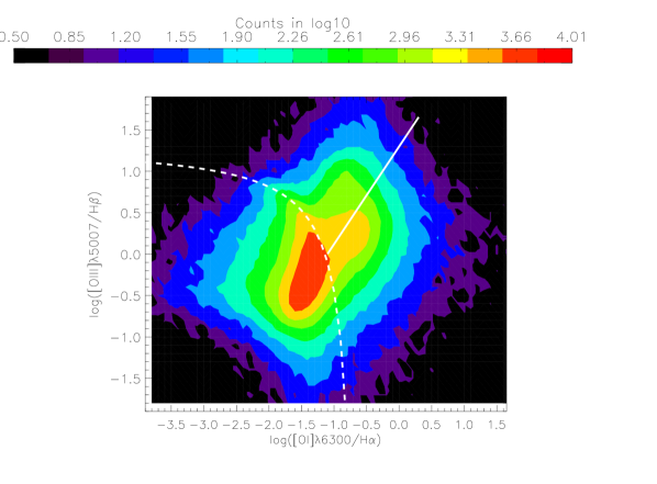
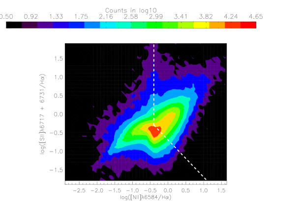
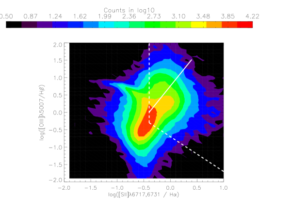
Figure 1: Diagnostic diagrams log([O iii]$\lambda$5007/H$\beta$) versus log([O i]$\lambda$6300/H$\alpha$, log([S ii]$\lambda\lambda$6716+31/H$\alpha$) versus log[N ii]$\lambda$6584/H$\alpha$, log([O iii]$\lambda$5007/H$\beta$) versus log[N ii]$\lambda$6584/H$\alpha$ and log([O iii]$\lambda$5007/H$\beta$) versus log([S ii]$\lambda\lambda$6716+31/H$\alpha$). The logarithm of the number of compiled SDSS objects (see Sect. 2) are shown according to their positions in each panel.

2.1 Observational data

In order to produce a sample of type 2 AGNs with observational intensities of narrow optical emission-lines, we used the measurements of the Sloan Digital Sky Survey (SDSS, York et al. 2000) DR7 data made available by MPA/JHU group. The procedure of measuring the emission-line intensities is described in details by Tremonti et al. (2004). The data produced by MPA/JHU are corrected for foreground (galactic) reddening using the the methodology presented by O’Donnell (1994).

In the SDSS-DR7 database there are 927 552 objects with signal-to-noise ratio (S/N) larger than 2 and redshift $z\><0.7$, in which 778 695 objects of these have estimation of stellar mass. In order to keep up the consistency of our analysis with our previous works (e.g. Pérez-Montero et al. 2019; Dors et al. 2015), we selected only the objects which have, at least, the [O ii]$\lambda 3727$, H$\beta$, [O iii]$\lambda 5007$, [O i]$\lambda 6300$, H$\alpha$, [N ii]$\lambda 6584$, and [S ii]$\lambda\lambda$6717,31 emission-lines measured. By adopting this procedure, our sample was reduced to 538 878 objects, mainly due to the requirement of having the [O ii]$\lambda 3727$ line measured.

Subsequently, in order to classify objects as AGN-like and as H ii-like, we used the standard Baldwin-Phillips-Terlevich (BPT) diagrams (Baldwin et al., 1981; Veilleux & Osterbrock, 1987). We used the criteria proposed by Kewley et al. (2001) and Pérez-Montero et al. (2013), which states that AGN-like are the ones that satisfy:

$$\scriptstyle\rm log([O\>III]\lambda 5007/H\beta)\>>\>\frac{0.61}{log([N\>II]\lambda 6584/H\alpha)-0.47}+1.19,$$ (1)

$$\scriptstyle\rm log([O\>III]\lambda 5007/H\beta)\>>\>\frac{0.72}{log([S\>II]\lambda\lambda 6717+31/H\alpha)-0.32}+1.30,$$ (2)

$$\scriptstyle\rm log([O\>III]\lambda 5007/H\beta)\>>\>\frac{0.73}{log([O\>I]\lambda 6300/H\alpha)+0.59}+1.33,$$ (3)

and

$$\scriptstyle\rm log([N\>II]\lambda 6584/H\alpha)\>>\>-1.05\>\times\>log([S\>II]\lambda\lambda 6717+31/H\alpha).$$ (4)

The “composite” objects as defined in Kewley et al. (2006) are not included in the sample.

In Figure 1, we present the diagnostic diagrams for the selected galaxies from the SDSS-DR7 (Abazajian et al., 2009) with the number of objects in each region according to the above criteria. These panels thus show the known results based on this sample, according to the SDSS-DR7 data, there is a larger number of H ii-like objects than AGN-like ones (e.g. Brinchmann et al. 2004; Zhang et al. 2013). We applied the criterion (also shown in Fig. 1) proposed by Kewley et al. (2006) to the selected sample to separate AGN-like and Low-ionization nuclear emission-line region (LINER) objects. The criterion establishes that objects with

$$\scriptstyle\rm log([O\>III]\lambda 5007/H\beta)\><\>1.30+1.18\>\times\>log([O\>I]\lambda 6300/H\alpha)$$ (5)

and

$$\scriptstyle\rm log([O\>III]\lambda 5007/H\beta)\><\>0.76+1.89\>\times\>log([S\>II]\lambda\lambda 6717+31/H\alpha)$$ (6)

are candidates to be AGN-like objects (including, for instance,  Seyfert 1s, Seyfert 2s, quasars, H ii-like objects with very strong winds and shocks), otherwise they are candidates to be LINERs.

As discussed above, the main interest in this paper is to address the study of AGNs. For this reason, we selected all objects that appear simultaneously above the dashed lines in the four panels of Figure 1. In total, there are 69,517 objects that satisfying the criteria presented by Kewley et al. (2001, 2006) and Pérez-Montero et al. (2013).

The classification criteria for separating objects according to their main ionization mechanisms presented previously and based on BPT diagrams are defined for objects at redshifts $z\sim 0$. However, Kewley et al. (2013) showed that the demarcation lines in optical diagnostic diagrams change as a function of cosmic time, since interstellar medium conditions are more extreme and it is expected harder ionizing radiation from stellar clusters (ionizing source of H ii-like objects) at high redshifts than those in local galaxies. Nevertheless, such as pointed by these authors, galaxy properties practically do not change for $z\><\>1$. The maximmum value of the redshift for the objects in our sample is $\sim 0.37$. Therefore, the cosmic evolution does not influence our classification.

For the selected objects, all emission line-fluxes were divided by the corresponding H$\beta$ flux. Next, we compiled from the NED/IPAC (NASA/IPAC Extragalactic Database) two catalogues containing basic information (classification) about Seyfert 1 and Seyfert 2 galaxies. In total, there are 10,054 classified as Seyfert 1 and 4,258 as Seyfert 2 AGNs. As the NED/IPAC provides a name of SDSS and the Garching’s database the objID, we matched them using the field objID supplied in both databases. We use the SDSS objID provided by both the NED/IPAC and the Garching databases to match the data. In this way, we found 112 Seyfert 1s and 463 Seyfert 2s.

The reddening correction was carried out comparing the observed H$\alpha$/H$\beta$ ratio with the theoretical value of 2.86 (Hummer & Storey, 1987), obtained for the Case B, considering an electron density of 100 $\rm cm^{-3}$ and an electron temperature of 10 000 K. We assumed the Galactic extinction law by Miller & Mathews (1972) with the ratio of total to selective extinction R_v=3.2. For ten objects the H$\alpha$/H$\beta$ were found to be lower than 2.86. Taking into account the errors in the measurements, for seven of them that present a reddening correction C(H$\beta$) between $-0.2$ and 0, we assumed it is equivalent to zero, and hence we did not apply any reddening correction. We take off from our sample the other three objects with C(H$\beta$) lower than $-0.2$. The stellar mass range of our sample is $9.4\>\la\>\log(M_{*}/\rm M_{\odot})\>\la\>11.6$, somewhat wider than the one considered by Thomas et al. (2019), who found that the oxygen abundance increases by $\rm\Delta(O/H)\sim 0.1$ dex as a function of the host galaxy stellar mass over the $10.1\>\la\>\log(M_{*}/\rm M_{\odot})\>\la\>11.3$ range.

The $M_{*}$ determination of the objects in our sample is based on a comparison between theoretical spectra from stellar population synthesis (SSP) codes with the SDSS $z$-band luminosities carried out by Tremonti et al. (2004) and Kauffmann et al. (2003). The errors associated to the $M_{*}$ determinations are mainly due to star-formation histories, ages, metallicities and extinction assumed in the SSPs fitting, which may differ from those of galaxies. In general, it is assumed the $M_{*}$ error is of the order of 0.2 dex (e.g. Maiolino et al. 2008; Taylor et al. 2011).

For the resulting Seyfert 2 AGNs sample, reddening corrected intensities (in relation to H$\beta$=1.0) of the [O ii]$\lambda$3726+3729, [Ne iii]$\lambda$3869, [O iii]$\lambda$4363, [O iii]$\lambda$5007, He I$\lambda$5876, [O i]$\lambda$6300, [N ii]$\lambda$6584, [S ii]$\lambda$6716, [S ii]$\lambda$6731 and [Ar iii]$\lambda$7135 emission-lines, redshifts ($z\>\la\>0.4)$, reddening correction C(H$\beta$), the electron density (in units of particles per cm³, see Sec. 3) are listed in a Table only available in online version. We take as zero the emission-line intensities that in the SDSS database have values lower than zero.

2.2 Aperture effects

The estimation of the physical properties of objects with different redshifts whose data were obtained by instruments with fixed aperture, such as the objects from the SDSS, are subject to some degree of uncertainty. Kewley et al. (2005) investigated the effect of aperture size on the star formation rate, $Z$ and reddening determinations for galaxies with distinct morphological type. Concerning the metallicity, Kewley et al. (2005) found that for aperture capturing less than $20\%$ of the total galaxy emission, the derived metallicity can differ by a factor of 0.14 dex from the value obtained when the total galaxy emission is considered.

In our case, only properties of the nuclear region are being considered, therefore, the aperture effect can not be so important. The diameter of the SDSS optical fibers is $\sim 3$^′′ , which implies that we are considering fluxes only emitted by the nuclear regions of the galaxies in the sample. In fact, our sample of 463 Seyfert 2 galaxies have redshifts in the range $0.03\>\la\>z\>\la\>0.37$, assuming a spatially flat cosmology with $H_{0}$ = 71 $\rm km\>s^{-1}Mpc^{-1}$, $\Omega_{m}=0.270$, and $\Omega_{\rm vac}=0.730$ (Wright, 2006), which corresponds to a physical scale (D) in the center of the disk of each galaxy in the range $\rm 50\>\la\>D(pc)\>\la\>660$, i.e. the emission is mainly from the AGN. For example, Storchi-Bergmann et al. (2007) showed that the highest [N ii]$\lambda$6584/H$\alpha$ line ratio in the nuclear region of NGC 6951 (LINER/Seyfert nuclei) is within a nuclear radius with $\sim\>100$ pc. Thus, for the farthest objects of our sample, the measured fluxes are emitted mainly by the AGN because the flux from (circum)nuclear star-forming regions, if present, have low contribution to the total flux. The support for this assertion was found, recently, by Thomas et al. (2019). These authors showed that the aperture effect is not important on $Z$ estimations in a similar AGN sample like the one being considered in this paper, once similar mass-metallicity relations for galaxies in four different redshift bins were derived in their analysis. However, Thomas et al. (2018) pointed out that a mixing of AGN and H ii regions emission is expected in the majority of AGNs (see also D’Agostino et al. 2019 and reference therein).

For the nearest objects, we could be estimating the metallicity only for the central part of the AGNs and the metallicity of the entire AGN can be different from this little region. Abundance studies of spatially resolved AGNs are (still) seldom found in the literature and not conclusive results have been obtained. For example, optical data of the nuclear region of the Seyfert 2 galaxy Markarian 573 obtained by Revalski et al. (2018) and Thomas et al. (2018) showed that the oxygen abundance is almost constant, with variations not larger than 0.10 dex along the central region. On the other hand, Thomas et al. (2018) found for two (NGC 2992 and ESO 138-G010) of the four objects analysed a steep metallicity gradients from the nucleus into the ionization cones, with $(Z/Z_{\odot})$ ranging from $\sim 0.5$ (in the outer regions) to $\sim 2$ (in the nucleus).

In order to explore the presence of an aperture effect on our oxygen abundance determinations, in the lower panel of Fig. 2, we plotted for each object of our sample the oxygen abundance values estimated using the calibration by Castro et al. (2017) versus the redshift, considering the redshift bins $z=0.0-0.1$, $z=0.1-0.2$ and $z\>>\>0.2$. We calculated the average and standard deviation of 12+log(O/H) and $z$ for each bin. Since it is not expected a significant chemical evolution over $z=0-0.4$, any systematic difference in the averages could be due to aperture effects. As can be seen in Fig. 2, the average oxygen abundances are similar for all the redshift bins ($\approx 8.64$ dex). In the upper panel of Fig. 2, we plotted for each object of our sample the electron densities ($N_{\rm e}$) as a function of the redshift and the average density values, with the standard deviations, for the same redshift bins definied above. Densities were estimated from the [S ii]$\lambda$6716/$\lambda$6731 emission-line ratio as described in Sec. 3. Since the electron densities in AGNs are higher by about a factor of 2 than those estimated for H ii regions (see e.g., Copetti et al. 2000; Kennicutt et al. 2003; Dors et al. 2014; Sanders et al. 2016), it is expected that if there is a significant contribution to the sulfur emission by H ii regions in the SDSS fluxes, a $N_{\rm e}$ decrement with the $z$ increases would be found. As can be seen in the upper panel of Fig. 2, such as for the O/H, the $N_{\rm e}$ average values in the different bins are very similar ($\approx 650\>\rm cm^{-3}$), indicating that this parameter does not change with the redshift. Therefore, we assume that aperture effects are not significant for the parameter estimations of the objects in our sample.

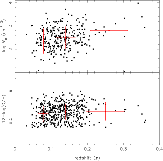
Figure 2: Bottom panel: Oxygen abundance [in units of 12+log(O/H)] versus the redshift for our sample of AGNs (see Sect. 2). The oxygen abundance was calculated using the calibration proposed by Castro et al. (2017). Red points represent the average and their error bars the standard deviation for the redshift bins $z=0.0-0.1$ and $z=0.1-0.2$. Top panel: Same than the bottom panel but for the logarithm of the electron density ($N_{\rm e}$).

Concerning the stellar mass of the galaxies in our sample, it is expected that due to aperture effects, it increases with $z$. This happens because as the $z$ increases, the projected SDSS fiber covers a larger galaxy portion and, hence, we are estimating the galaxy mass taking into account a larger area (for a full description see, for example, Tremonti et al. 2004). In order to show that, in Fig. 3, the logarithm of the stellar mass (in units of $\rm M_{\odot}$) versus the redshift for the objects in our sample is presented, where a clear correlation is appreciated. This result indicates that to obtain a reliable mass-metallicity relation it is necessary to consider different redshift bins (see, e.g. Maiolino et al. 2008; Kewley & Ellison 2008).

Figure 3: Logarithm of the stellar mass (in units of $\rm M_{\odot}$) versus the redshit for our objects sample (see Sect. 2).

3 Metallicity estimations

We used the emission-line intensities, listed in the online Table, to estimate the total oxygen abundances relative to hydrogen abundance (generally used as metallicity tracer) of the NLRs for the objects in our sample of AGNs. All the methods used in this work were taken from the literature and are described as it follows.

3.1 $T_{\rm e}$-method

This method consists of calculating the oxygen abundance in relation to the hydrogen one (O/H) using direct measurements of the electron temperature of the gas phase. We followed the methodology described in Dors et al. (2015) which is based on Pérez-Montero & Contini (2009), Hägele et al. (2008), Pérez-Montero et al. (2007) and Pérez-Montero & Díaz (2003).

The electron temperature in the high ionization zone of the gas phase, referred to $t_{3}$, for each object of the sample, was calculated from the observed line-intensity ratio $R_{\rm O3}$=[O iii]($\lambda 4959\>+\>\lambda 5007)/\lambda 4363$ and using the expression

$$t_{3}=0.8254-0.0002415R_{\rm O3}+\frac{47.77}{R_{\rm O3}},$$ (7)

where $t_{3}$ is in units of $10^{4}$ K. This relation is valid for the range of $0.7\>\la\>t_{3}\>\la\>2.3$.

The electron temperature value for the low ionization zone, referred to $t_{2}$, was derived from the theoretical relation

$$t_{2}^{-1}\,=\,0.693\,t_{3}^{-1}+0.281.$$ (8)

The electron density ($N_{\rm e}$), for each object, was calculated from the $R_{S2}=$[S ii]$\lambda 6716/\lambda 6731$ line ratio, using the IRAF/temden task and assuming the $t2$ value obtained from Eq. 8. It was possible to compute $N_{\rm e}$ for 295 ($\sim 64\%$) objects of our sample. For the other objects $N_{\rm e}=650\>\rm cm^{-3}$ was assumed, the average value derived for our sample.

The $\rm O^{++}$ and $\rm O^{+}$ ionic abundances in relation to $\rm H^{+}$ abundance were computed through the relations:

$$12+\log(\frac{{\rm O^{++}}}{{\rm H^{+}}})\!\!\! = \!\!\!\log\big{(}\frac{I(4959)+I(5007)}{I{\rm(H\beta)}}\big{)}+6.144$$ (9)

$$\!\!\!+\frac{1.251}{t_{3}}-0.55\log t_{3}$$

and

$$12+\log(\frac{{\rm O^{+}}}{{\rm H^{+}}})\!\!\! = \!\!\!\log\big{(}\frac{I(3727)}{I{\rm(H\beta)}}\big{)}+5.992$$ (10)

$$\!\!\!+\frac{1.583}{t_{2}}-0.681\log t_{2}+\log(1+2.3n_{\rm e}),$$

where $n_{\rm e}$ is the electron density $N_{\rm e}$ in units of 10 000 $\rm cm^{-3}$.

Finally, the total oxygen abundance in relation to hydrogen one (O/H) was calculated assuming

$$\rm\frac{O}{H}=\frac{O^{+}}{H^{+}}+\frac{O^{++}}{H^{+}}.$$ (11)

The expression above assumes that the Ionization Correction Factor (ICF) for the oxygen is equal to 1, even though ions with higher ionization states are observed in other spectral bands as, for instance, X-rays (e.g. Cardaci et al. 2009, 2011; Bianchi et al. 2010; Bogdán et al. 2017), indicating that there could be a significant contribution of them. We point out this issue in the work by Pérez-Montero et al. (2019). A model-base estimation of the oxygen ICF for NLRs will be addressed in a forthcoming work even though in Sec. 5 we provided a brief review of alternative ICF(O) values.

Due to the fact that the [O iii]$\lambda$4363 line is weak or not observable in the majority of AGNs and, due to the validity range of the Equation 7, it was possible to apply the $T_{e}$-method only in 154 ($\sim 33\%$) objects of our sample.

3.2 Strong-line method

3.2.1 Storchi-Bergmann et al. calibrations

Storchi-Bergmann et al. (1998) proposed the first calibrations between the metallicity [$Z\rm=12+\log(O/H)$] and the intensities of narrow optical emission-line ratios of AGNs. These calibrations are based on results of photoionization models built with the Cloudy code. The calibrations proposed by these authors are:

$$\begin{array}[]{l@{}l@{}l}\rm(O/H)_{SB98,1}&=&8.34+(0.212\,x)-(0.012\,x^{2})-(0.002\,y)\\ &+&(0.007\,xy)-(0.002\,x^{2}y)+(6.52\times 10^{-4}\,y^{2})\\ &+&(2.27\times 10^{-4}\,xy^{2})+(8.87\times 10^{-5}\,x^{2}y^{2}),\\ \end{array}$$ (15)

where $x$ = [N ii]$\lambda$$\lambda$6548,6584/H$\alpha$ and $y$ = [O iii]$\lambda$$\lambda$4959,5007/H$\beta$ and

$$\begin{array}[]{lll}(\rm{O/H})_{{\rm SB98,2}}&=&8.643-0.275\,u+0.164\,u^{2}\\ &+&0.655\,v-0.154\,uv-0.021\,u^{2}v\\ &+&0.288v^{2}+0.162uv^{2}+0.0353u^{2}v^{2},\\ \end{array}$$ (19)

where $u$ = log([O ii]$\lambda$$\lambda$3727,3729/[O iii]$\lambda$$\lambda$4959,5007) and $v$ = log([N ii]$\lambda$$\lambda$6548,6584/H$\alpha$). The term O/H above corresponds to 12+log(O/H). Both calibrations are valid for $\rm 8.4\>\lid\>12+log(O/H)\>\lid\>9.4$ and were obtained adoptating in the models the (N/O)-(O/H) abundance relation derived for nuclear starbursts by Storchi-Bergmann et al. (1994).

As pointed out by Storchi-Bergmann et al. (1998), the O/H should be corrected in order to take into account the electron density ($N_{\rm e}$) effects. Hence, the final value for the ratio O/H ratio is given by the relation below:

$${\rm(O/H)_{final}=[(O/H)}-0.1\>\times\>\log(N_{\rm e}/300({\rm cm^{-1}})].$$ (20)

3.2.2 Castro et al. calibration

Castro et al. (2017) proposed a semi-empirical calibration between the metallicity $Z$ and the line ratio $N2O2$=log([N ii]$\lambda$6584/[O ii]$\lambda$3727). This calibration was performed determining $Z$ of a sample of 58 Seyfert 2 AGNs through a diagram containing the observational data and the results of a grid of photoionization models obtained with the Cloudy code (Ferland et al., 2013). In these models, the (N/O)-(O/H) abundance relation derived for H ii regions by Dopita et al. (2000) was assumed. These authors found

$$\begin{array}[]{lll}(Z/Z_{\odot})\!\!\!&=&\!\!\!1.08(\pm 0.19)\times N2O2^{2}+1.78(\pm 0.07)\times N2O2\\ &&+1.24(\pm 0.01).\\ \end{array}$$ (23)

The oxygen abundance is obtained by

$$12+\log({\rm O/H})=12+\log[(Z/Z_{\odot})\times 10^{-3.31}],$$ (24)

where the solar oxygen abundance $\rm\log(O/H)=-3.31$ derived by Allende Prieto et al. (2002) was considered.

3.2.3 H ii-Chi-mistry code

The H ii-Chi-mistry code (hereafter HCm), proposed by Pérez-Montero (2014), establishes a bayesian-like comparison between the predictions from a grid of photoionization models covering a large range of input parameters and using the lines emitted by the ionized gas. This method has the advantage of not assuming any fixed relation between secondary and primary elements (e.g. N-O relation) considered in most of the calibrations such as the ones proposed by Storchi-Bergmann et al. (1998) and Castro et al. (2017). In Pérez-Montero et al. (2019) this code was adapted to be used in the Seyfert 2 AGNs and this last version is the one considered here.

Thomas et al. (2019) proposed another Bayesian code (NebulaBayes) presented initially by Blanc et al. (2015) and based on a comparison between observed emission-line fluxes and photoionization model grids which helped to obtain robust measurements of abundances in the extended narrow-line regions (ENLRs) of AGNs. This code produces very similar O/H values to those found using the calibration of Castro et al. (2017), such as pointed out by Thomas et al. (2019). Therefore, by simplicity, we do not consider it here.

The oxygen abundance estimations for each object of the sample computed by using the methods above are listed in the online Table.

4 Results

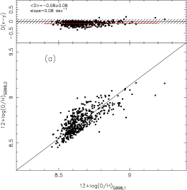
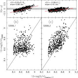
Figure 4: Comparison between oxygen abundances [in units of 12+log(O/H)] computed using the observational data described in Sect. 2 and the methods listed in Sect. 3. Bottom panel of each plot is the comparison between two estimations. Solid line represents the equality between these. Top panel is the difference (D=x-y) between the estimations. Black line represents the null difference while red line represents a linear regression to these differences whose slope is indicated. The average difference ($\rm<D>$) is indicated in each plot. The dashed area indicates the uncertainty of $\pm 0.1$ assumed in the oxygen abundance estimations. Panel (a): Comparison between oxygen abundances computed via Eq.s 19 versus Eqs. 15 proposed by Storchi-Bergmann et al. (1998). Panel (b): Such as panel (a) but for Eq. 19 (referred to SB98,1) versus O/H estimations via Castro et al. (2017) calibration. Panel (c): Such as panel (a) but for Eq. 15 (referred to SB98,2) versus O/H estimations via Castro et al. (2017) calibration. Panel (d): Such as panel (a) but for O/H estimations via Castro et al. (2017) versus the ones via $T_{\rm e}$-method. Panel (e): Such as panel (a) but for O/H estimations via Hii-Chi-mistry (HCm) code versus the ones via Castro et al. (2017) calibration.

We used the observational data described in Sect. 2 in order to compare the oxygen abundance estimations computed using the aforementioned methods.

For SFs, the metallicity or oxygen abundance is defined by estimations based on the classical $T_{\rm e}$-method and any calibration must be tested comparing its estimations to this bona fide method. The accuracy of the $T_{\rm e}$-method is also supported by the agreement between oxygen abundances in nebulae located in the solar neighborhood and those derived from observations of the weak interstellar O i$\lambda$1356 line towards the stars (see Pilyugin 2003 and references therein), although determinations of stellar oxygen abundances following different approaches have led to distinct values with variations of up to $\sim 3$ dex, as showed by Caffau et al. (2015). However, as pointed out by Dors et al. (2015), the $T_{\rm e}$-method, in its usual application form, does not work for AGNs and, obviously, it can not be used as reference for this kind of object. In other words, there is no consensus on which is the best method to estimate O/H (or $Z$) in AGNs. Therefore, we compared O/H estimations based on the methods listed above to know the discrepancy between them.

The uncertainty in the metallicity estimations (traced by the O/H abundance) depends on which method is considered. For example, for the $T_{\rm e}$-method the uncertainty is about 0.1 dex (e.g. Pilyugin 2000; Kennicutt et al. 2003; Hägele et al. 2008) while for strong-line calibrations is in order of 0.2 dex (Denicoló et al., 2002). In this paper, we assume that the uncertainty in O/H estimations is 0.2 dex, the highest uncertainty value considered in H ii region abundance studies.

We start the analysis comparing the O/H estimations computed from the two Storchi-Bergmann et al. (1998) calibrations (SB98,1 and SB98,2). In Fig. 4, panel (a), the oxygen abundances calculated using SB98,2 versus SB98,1 are shown. A good agreement between the estimations can be seen, with SB98,1 producing somewhat lower values ($-0.08$ dex) than the ones from SB98,2. Storchi-Bergmann et al. (1998) carried out a similar comparison but using only 7 objects and these authors found differences of about $-0.1$ dex, about the same value derived by us. More recently, Dors et al. (2015) compared O/H values predicted by photoionization models with estimations obtained from Storchi-Bergmann et al. (1998) calibrations, in an O/H versus $R_{23}$=([O ii]$\lambda$3727+[O iii]$\lambda$4959+$\lambda$5007)/H$\beta$ plot, and these authors found a better consistency with the SB98,1. Dors et al. (2015) used a small sample (47 Seyfert 2s). However, taking into account the uncertainty of 0.2 dex, both Storchi-Bergmann et al. (1998) calibrations produce similar abundances.

In Fig. 4, panels (b) and (c), we compare the estimations via the two Storchi-Bergmann et al. (1998) calibrations with the ones obtained via Castro et al. (2017) calibration. We can see that, despite the difference between the estimations, the average difference is lower than the uncertainty. However, a systematic discrepancy is clearly derived, in the sense that Storchi-Bergmann et al. (1998) calibrations produce lower and higher values for the high ($\rm 12+\log(O/H)\>\ga\>8.6$) and low ($\rm 12+\log(O/H)\>\la\>8.6$) metallicity regimes, respectively, being this behavior more clear when the SB98,1 is considered. One can note that the difference between estimations from Castro et al. (2017) and from Storchi-Bergmann et al. (1998) calibrations reach up to 0.5 dex for the lowest metallicity values ($\rm 12+\log(O/H)\approx 7.5$). Castro et al. (2017) found a similar result, although most of the objects considered by these authors are located around 12+log(O/H)=8.7, i.e. the solar abundance (Allende Prieto et al., 2002). In Fig. 4, panel (d), the estimations by the calibration by Castro et al. (2017) versus those obtained via $T_{\rm e}$-method are shown. A systematic difference is found, ranging from $\sim 0$ for the highest O/H values to $\sim 2$ dex for the lowest ones. The average difference is about $-0.6$ dex, a lower value than the one ($-0.8$ dex) found by Dors et al. (2015), who compared O/H estimations derived using Storchi-Bergmann et al. (1998) calibrations with those via $T_{\rm e}$-method. In Fig. 4, panel (e), the values derived from Castro et al. (2017) are compared to those from HCm code (Pérez-Montero et al. 2019), where, despite the difference between estimations is about zero, a systematic difference is found.

5 Discussion

It is known that in SFs many strong-line methods calibrated using theoretical models overestimate $Z$ as compared to the results from the $T_{\rm e}$-method. For example, Yin et al. (2007) determined the gas-phase oxygen abundance using the $T_{\rm e}$-method for a sample of 695 star-forming galaxies and H ii regions with reliable detections of [O iii]$\lambda$4363. These authors found that the oxygen abundances derived using certain theoretical calibrations are between 0.06 and 0.20 tex larger than those derived using the $T_{\rm e}$-method. Kewley & Ellison (2008) analyzed the mass-metallicity (M–Z) relation of star-forming galaxies, whose data were taken from the SDSS (York et al., 2000) database, and found metallicity discrepancies for a fixed value of $M$ of up to $\sim 0.7$ dex when distinct theoretical and empirical strong-line methods are considered.

Regarding AGNs, when only strong-line methods are considered, discrepancies of up to $\sim 0.8$ dex were found when distinct methods are used to estimate O/H in NLRs of Seyfert 2s, being these discrepancies higher for the low metallicity regime ($\rm 12+\log(O/H)\>\la\>8.5$). The discrepancy found when the Storchi-Bergmann et al. (1998) and Castro et al. (2017) calibrations are considered are due to the different N-O abundance relations assumed in the photoionization models by these authors, which have a more important effect for the low metallicity regime, mainly because [N ii] lines are used in both calibrations (Pérez-Montero & Contini, 2009). The discrepancy between the $Z-N2O2$ calibration (Castro et al., 2017) and those derived from the bayesian code HCm (Pérez-Montero et al., 2019) can also be due to a fixed N-O relation. In fact, as mentioned, Castro et al. (2017) assumed photoionoization models with fixed N-O relation, taken from H ii chemical abundance estimations carried out by Dopita et al. (2000), while in the bayesian HCm approach this relation is not fixed.

The $T_{\rm e}$-method produces, possibly, unreal O/H subsolar estimations and the origin of these low values could arise from the supposition that the ICF for the oxygen is equal to 1 (Eq. 11). There are no equations to estimate oxygen ICFs for NLRs of type 2 AGNs in the literature. For Planetary Nebula (PN), the following expression to estimate ICF(O) was proposed by Torres-Peimbert & Peimbert (1977):

$$\rm ICF(O)=\frac{N(He^{+}+He^{2+})}{N(He^{+})},$$ (25)

where N represents the abundance (see also Alexander & Balick, 1997; Izotov et al., 2006; García-Rojas & Esteban, 2007; Delgado-Inglada et al., 2014). This equation provides estimated values for the ICF of PNs in the range between $\sim 1$ and 1.6 (e.g. Krabbe & Copetti, 2006). For H ii regions, low ICF(O) has been also derived (e.g. Izotov et al. 2006). Unfortunately, for the objects in our sample it was not possible to apply Eq. 25 because the He ii$\lambda$4686 emission line, necessary to calculate $\rm N(He^{2+})$, was not measured. For this reason, we used the sample of 47 type 2 AGNs compiled by Dors et al. (2015) in order to calculate the ICF(O). We used the expressions by Izotov et al. (1994):

$${\rm\frac{N(He^{+})}{N(H^{+})}}=0.738\>t^{0.23}\>\frac{I(\lambda 5876)}{I(\rm H\beta)}$$ (26)

and

$${\rm\frac{N(He^{2+})}{N(H^{+})}}=0.084\>t^{0.14}\>\frac{I(\lambda 4686)}{I(\rm H\beta)},$$ (27)

where $t=t_{3}$ is assumed. It was possible to calculate the ICF(O) only for 33 objects since the He i$\lambda$5876 and He ii$\lambda$4686 emission lines are not available for all these 47 objects.

Figure 5: Histogram containing the ICF(O) calculated using the Eqs. 25 and 26 for 33 type AGNs whose data were compiled by Dors et al. (2015).

In Fig. 5 a histogram with the ICF(O) distribution is shown. It can be seen that most part of the objects have $\rm ICF(O)\>\la\>1.4$, with an average value of $1.23\pm 0.15$. This indicates an average oxygen abundance correction of about 0.1 dex, i.e. the oxygen in AGNs is mainly in $\rm O^{+}$ and $\rm O^{++}$ ionic stages. Therefore, the supposition of ICF(O)=1 would not be the cause of the discrepancy derived between O/H estimations based on $T_{\rm e}$-method and on strong-line methods. It must be noted that, as we pointed above, we are using an ICF(O) derived for Planetary Nebulae.

In Fig. 6 we show the histograms of the oxygen abundances in the selected sample derived following the distinct methods described in Sect. 3, as compared with the abundances obtained by extrapolating the O/H radial distributions to the nuclear region (containing AGN and SF region) of a sample of spiral disks obtained by Pilyugin et al. (2004), who used the $P$-method (Pilyugin, 2001). These extrapolated estimations can be understood as an independent ones, which do not suffer effects of intrinsic uncertainties present in photoionization models or the limitations of the $T_{\rm e}$-method. We can see that strong-line methods produce similar oxygen abundance distributions, with the most frequent value around of 8.7, the solar abundance. On the other hand, the $T_{\rm e}$-method produces, in most cases, sub-solar abundances. We list in Table 1 the minimum, maximum and average values of the distributions of oxygen abundances derived using the distinct methods described in Sect. 3. From the above results one can conclude that, considering the uncertainty of 0.2 dex in the oxygen estimations, all strong-line methods available in the literature produce similar oxygen abundance distributions when a large and homogeneous sample of data are used. The average maximum value of the oxygen abundance for our sample of Seyfert 2 AGNs through the strong-line methods is $\rm 12+\log(O/H)\sim 9.1$, which is slightly higher than the one derived for star-forming galaxies ($\sim 8.95$ dex) by Pilyugin et al. (2007). This agreement suggests that there is no extraordinary chemical enrichment of the NLRs of AGNs (see also Dors et al. 2015), as also pointed out from the comparison between N and O abundances both in AGNs and in SFs by Dors et al. (2017) and Pérez-Montero et al. (2019).

Figure 6: Histogram containing the oxygen abundance distributions for NLRs of AGNs and based on distinct methods as indicated and described in Sect. 3. Extrapolation estimations refers to the extrapolated values to the nuclear region obtained using the radial oxygen gradient derived by Pilyugin et al. (2004) for a sample of spiral galaxies.

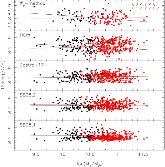
Figure 7: Metallicity of the NLR for the sample of AGNs (see Sect. 2) versus the logarithm of stellar mass $M_{*}$ (in units of solar mass ($\rm M_{\odot}$) of the hosting galaxy. The methods considered to obtain the $Z$ estimations are indicated in each plot. The curves represent the fitting of the Eq. 28 on the points whose coefficients are listed in Table 1. Different color correspond to estimations for two redshift intervals indicated in the top panel.

Table 1: Minimum, maximum and the average oxygen abundance values derived by the use of the distintive methods descrived in Sect. 3 and indicated in the first column. The $A$ and $B$ values correspond to the parameter fittings of the Eq. 28 on the estimations showed in Fig. 7 for the redshift bins $z=0.0-0.1$ and $z=0.1-0.2$.

	12+log(O/H)				$z=0.0-0.1$			$z=0.1-0.2$
Method	Min.	Max.	Aver.		$A$	$B$		$A$	$B$
$N2O2$	8.39	8.99	8.64$\pm 0.13$		$0.0017\pm 0.0019$	$8.44\pm 0.20$		$-0.0007\pm 0.0015$	$8.73\pm 0.18$
HCm	7.17	9.08	8.71$\pm 0.30$		$-0.0050\pm 0.0004$	$9.20\pm 0.47$		$0.0024\pm 0.0034$	$8.35\pm 0.41$
SB98,1	8.43	9.18	8.61$\pm 0.11$		$-0.0007\pm 0.0015$	$8.69\pm 0.17$		$0.0007\pm 0.0013$	$8.53\pm 0.16$
SB98,2	8.42	9.18	8.69$\pm 0.13$		$-0.0005\pm 0.0001$	$8.74\pm 0.21$		$-0.0011\pm 0.0015$	$8.83\pm 0.18$
$T_{\rm e}$-method	7.43	9.13	8.07$\pm 0.34$		$-0.0144\pm 0.0081$	$9.67\pm 0.86$		$0.0006\pm 0.0006$	$7.97\pm 0.79$

We also derive the relation between the stellar mass ($M_{*}$) of the host galaxy with the metallicity $Z$ of its AGN derived using the different methods analised in the present work. Recently, Thomas et al. (2019) found a mass metallicity (M–Z) relation for Seyfert 2 galaxies in the local Universe ($z\>\la 0.2$) while Matsuoka et al. (2018) found this relation for type 2 AGNs at $1.2\><\>z\><\>4.0$ (see also Dors et al. 2019). The different M–Z relations are shown in Fig. 7. For each M–Z plot we fit the expression

$$12+\log({\rm O/H})=A\times\left(\log\frac{M_{\star}}{M_{\odot}}\right)^{2}+B$$ (28)

which was adapted from Maiolino et al. (2008), who derived the M–Z relation for galaxies at different redshifts. The results of the fits are shown in Table 1 and presented in Fig. 7. We can see that the chemical abundances derived using strong-line methods do not show any correlation between the metallicity of the NLR and the stellar mass of the host galaxy.

6 Conclusion

We used observational emission line intensities of 463 confirmed AGNs taken from the SDSS DR7, whose classification as Seyfert 2 is available in the NED, to compare oxygen abundance in the NLRs of these objects obtained through the strong-line methods: two theoretical calibrations proposed by Storchi-Bergmann et al. (1998), the semi-empirical $N2O2$ calibration proposed by Castro et al. (2017), the bayesian H ii-Chi-mistry (HCm) code proposed by Pérez-Montero et al. (2019), as well as O/H values obtained by using the $T_{\rm e}$-method. We found that the two calibrations of Storchi-Bergmann et al. (1998) produce very similar oxygen abundance values from each other, with an average difference of 0.08 dex, a lower value than the one (0.2 dex) attributed to uncertainty in estimations via strong-line methods. The Storchi-Bergmann et al. (1998) calibrations and the HCm code produce lower and higher O/H values for the high ($\rm 12+\log(O/H)\>\ga\>8.6$) and low ($\rm 12+\log(O/H)\>\la\>8.6$) metallicity regimes in comparison to those derived by using the $N2O2$ calibration. These discrepancies are due to the relation between the nitrogen and oxygen abundances assumed in the photoionization models considered in the calibrations (methods). A sistematic difference between O/H values calculated via $T_{\rm e}$-method and via $N2O2$ calibration was found, ranging from $\sim 0$ for the highest O/H values to $\sim 2$ dex for the lowest ones. We showed that this difference can not be explained by taking into account the use of Ionization Correction Factors for the oxygen in the $T_{\rm e}$-method. We also analysed the influence of the use of the different strong-line methods on the derivation of the relation between the stellar mass of the galaxies ($M_{*}$) and the metallicity $Z$ (traced by the O/H abundance) of their AGNs. We did not find any correlation between $Z$ and $M_{*}$ and this result is independent of the method used to estimate the metallicity.

7 Acknowledgements

We thank the referee for helping to improve this paper with her/his constructive feedback. OLD and ACK thank FAPESP and CNPq for the finnancial support. Funding for the SDSS and SDSS-II has been provided by the Alfred P. Sloan Foundation, the Participating Institutions, the National Science Foundation, the U.S. Department of Energy, the National Aeronautics and Space Administration, the Japanese Monbukagakusho, the Max Planck Society, and the Higher Education Funding Council for England. The SDSS Web Site is http://www.sdss.org/. The SDSS is managed by the Astrophysical Research Consortium for the Participating Institutions. The Participating Institutions are the American Museum of Natural History, Astrophysical Institute Potsdam, University of Basel, University of Cambridge, Case Western Reserve University, University of Chicago, Drexel University, Fermilab, the Institute for Advanced Study, the Japan Participation Group, Johns Hopkins University, the Joint Institute for Nuclear Astrophysics, the Kavli Institute for Particle Astrophysics and Cosmology, the Korean Scientist Group, the Chinese Academy of Sciences (LAMOST), Los Alamos National Laboratory, the Max-Planck-Institute for Astronomy (MPIA), the Max-Planck-Institute for Astrophysics (MPA), New Mexico State University, Ohio State University, University of Pittsburgh, University of Portsmouth, Princeton University, the United States Naval Observatory, and the University of Washington. We also thank to Max-Planck-Institute for Astrophysics and John Hopkins University for Physical properties for galaxies and active galactic nuclei in the Sloan Digital Sky Survey: Data catalogues from SDSS studies at MPA/JHU. This research has made use of the VizieR catalogue access tool, CDS, Strasbourg, France (DOI : 10.26093/cds/vizier). The original description of the VizieR service was published in A$A$S 143, 23. This work has also made use of the computing facilities of the Laboratory of Astroinformatics (IAG/USP, NAT/Unicsul), whose purchase was made possible by the Brazilian agency FAPESP (grant 2009/54006-4) and the INCT-A.

References

- Abazajian et al. (2009) Abazajian K. N., Adelman-McCarthy J. K., Agüeros M. A., Allam S. S., Allende Prieto C., An D., Anderson K. S. J., Anderson S. F., Annis J., Bahcall N. A., et al. 2009, ApJS, 182, 543
- Alexander & Balick (1997) Alexander J., Balick B., 1997, AJ, 114, 713
- Allende Prieto et al. (2002) Allende Prieto C., Lambert D. L., Asplund M., 2002, ApJ, 573, L137
- Alloin et al. (1992) Alloin D., Bica E., Bonatto C., Prugniel P., 1992, A&A, 266, 117
- Baldwin et al. (2003) Baldwin J. A., Hamann F., Korista K. T., Ferland G. J., Dietrich M., Warner C., 2003, ApJ, 583, 649
- Baldwin et al. (1981) Baldwin J. A., Phillips M. M., Terlevich R., 1981, PASP, 93, 5
- Batra & Baldwin (2014) Batra N. D., Baldwin J. A., 2014, MNRAS, 439, 771
- Bianchi et al. (2010) Bianchi S., Chiaberge M., Evans D. A., Guainazzi M., Baldi R. D., Matt G., Piconcelli E., 2010, MNRAS, 405, 553
- Blanc et al. (2015) Blanc G. A., Kewley L., Vogt F. P. A., Dopita M. A., 2015, ApJ, 798, 99
- Bogdán et al. (2017) Bogdán Á., Kraft R. P., Evans D. A., Andrade-Santos F., Forman W. R., 2017, ApJ, 848, 61
- Brinchmann et al. (2004) Brinchmann J., Charlot S., White S. D. M., Tremonti C., Kauffmann G., Heckman T., Brinkmann J., 2004, MNRAS, 351, 1151
- Caffau et al. (2015) Caffau E., Ludwig H.-G., Steffen M., Livingston W., Bonifacio P., Malherbe J.-M., Doerr H.-P., Schmidt W., 2015, A&A, 579, A88
- Cardaci et al. (2011) Cardaci M. V., Santos-Lleó M., Hägele G. F., Krongold Y., Díaz A. I., Rodríguez-Pascual P., 2011, A&A, 530, A125
- Cardaci et al. (2009) Cardaci M. V., Santos-Lleó M., Krongold Y., Hägele G. F., Díaz A. I., Rodríguez-Pascual P., 2009, A&A, 505, 541
- Castellanos et al. (2002) Castellanos M., Díaz A. I., Terlevich E., 2002, MNRAS, 329, 315
- Castro et al. (2017) Castro C. S., Dors O. L., Cardaci M. V., Hägele G. F., 2017, MNRAS, 467, 1507
- Copetti et al. (2000) Copetti M. V. F., Mallmann J. A. H., Schmidt A. A., Castañeda H. O., 2000, A&A, 357, 621
- D’Agostino et al. (2019) D’Agostino J. J., Kewley L. J., Groves B. A., Medling A. M., Di Teodoro E., Dopita M. A., Thomas A. D., Sutherland R. S., Garcia-Burillo S., 2019, MNRAS, 487, 4153
- Delgado-Inglada et al. (2014) Delgado-Inglada G., Morisset C., Stasińska G., 2014, MNRAS, 440, 536
- Denicoló et al. (2002) Denicoló G., Terlevich R., Terlevich E., 2002, MNRAS, 330, 69
- Dhanda et al. (2007) Dhanda N., Baldwin J. A., Bentz M. C., Osmer P. S., 2007, ApJ, 658, 804
- Díaz et al. (2007) Díaz Á. I., Terlevich E., Castellanos M., Hägele G. F., 2007, MNRAS, 382, 251
- Dopita et al. (2000) Dopita M. A., Kewley L. J., Heisler C. A., Sutherland R. S., 2000, ApJ, 542, 224
- Dors & Copetti (2005) Dors J. O. L., Copetti M. V. F., 2005, A&A, 437, 837
- Dors et al. (2008) Dors J. O. L., Storchi-Bergmann T., Riffel R. A., Schimdt A. A., 2008, A&A, 482, 59
- Dors et al. (2014) Dors O. L., Cardaci M. V., Hägele G. F., Krabbe Â. C., 2014, MNRAS, 443, 1291
- Dors et al. (2015) Dors O. L., Cardaci M. V., Hägele G. F., Rodrigues I., Grebel E. K., Pilyugin L. S., Freitas-Lemes P., Krabbe A. C., 2015, MNRAS, 453, 4102
- Dors et al. (2019) Dors O. L., Monteiro A. F., Cardaci M. V., Hägele G. F., Krabbe A. C., 2019, MNRAS, 486, 5853
- Dors et al. (2017) Dors Jr. O. L., Arellano-Córdova K. Z., Cardaci M. V., Hägele G. F., 2017, MNRAS, 468, L113
- Dors et al. (2011) Dors Jr. O. L., Krabbe A., Hägele G. F., Pérez-Montero E., 2011, MNRAS, 415, 3616
- Ferland et al. (1996) Ferland G. J., Baldwin J. A., Korista K. T., Hamann F., Carswell R. F., Phillips M., Wilkes B., Williams R. E., 1996, ApJ, 461, 683
- Ferland et al. (2013) Ferland G. J., Porter R. L., van Hoof P. A. M., Williams R. J. R., Abel N. P., Lykins M. L., Shaw G., Henney W. J., Stancil P. C., 2013, RMXAA, 49, 137
- García-Rojas & Esteban (2007) García-Rojas J., Esteban C., 2007, ApJ, 670, 457
- Gelbord et al. (2009) Gelbord J. M., Mullaney J. R., Ward M. J., 2009, MNRAS, 397, 172
- Guseva et al. (2019) Guseva N. G., Izotov Y. I., Fricke K. J., Henkel C., 2019, A&A, 624, A21
- Hägele et al. (2008) Hägele G. F., Díaz Á. I., Terlevich E., Terlevich R., Pérez-Montero E., Cardaci M. V., 2008, MNRAS, 383, 209
- Hägele et al. (2006) Hägele G. F., Pérez-Montero E., Díaz Á. I., Terlevich E., Terlevich R., 2006, MNRAS, 372, 293
- Hamann & Ferland (1992) Hamann F., Ferland G., 1992, ApJ, 391, L53
- Hamann & Ferland (1993) Hamann F., Ferland G., 1993, ApJ, 418, 11
- Hamann et al. (2002) Hamann F., Korista K. T., Ferland G. J., Warner C., Baldwin J., 2002, ApJ, 564, 592
- Hummer & Storey (1987) Hummer D. G., Storey P. J., 1987, MNRAS, 224, 801
- Izotov et al. (2006) Izotov Y. I., Stasińska G., Meynet G., Guseva N. G., Thuan T. X., 2006, A&A, 448, 955
- Izotov et al. (1994) Izotov Y. I., Thuan T. X., Lipovetsky V. A., 1994, ApJ, 435, 647
- Kauffmann et al. (2003) Kauffmann G., Heckman T. M., et al. 2003, MNRAS, 341, 33
- Kennicutt et al. (2003) Kennicutt Jr. R. C., Bresolin F., Garnett D. R., 2003, ApJ, 591, 801
- Kewley et al. (2001) Kewley L. J., Dopita M. A., Sutherland R. S., Heisler C. A., Trevena J., 2001, ApJ, 556, 121
- Kewley & Ellison (2008) Kewley L. J., Ellison S. L., 2008, ApJ, 681, 1183
- Kewley et al. (2006) Kewley L. J., Groves B., Kauffmann G., Heckman T., 2006, MNRAS, 372, 961
- Kewley et al. (2005) Kewley L. J., Jansen R. A., Geller M. J., 2005, PASP, 117, 227
- Kewley et al. (2013) Kewley L. J., Maier C., Yabe K., Ohta K., Akiyama M., Dopita M. A., Yuan T., 2013, ApJ, 774, L10
- Krabbe & Copetti (2006) Krabbe A. C., Copetti M. V. F., 2006, A&A, 450, 159
- Lee et al. (2013) Lee J. C., Hwang H. S., Ko J., 2013, ApJ, 774, 62
- Liang et al. (2006) Liang Y. C., Yin S. Y., Hammer F., Deng L. C., Flores H., Zhang B., 2006, ApJ, 652, 257
- López-Sánchez & Esteban (2010) López-Sánchez Á. R., Esteban C., 2010, A&A, 517, A85
- Maiolino & Mannucci (2019) Maiolino R., Mannucci F., 2019, A&A Rev., 27, 3
- Maiolino et al. (2008) Maiolino R., Nagao T., Grazian A., Cocchia F., Marconi A., Mannucci F., Cimatti A., Pipino A., Ballero S., Calura F., Chiappini C., Fontana A., Granato G. L., Matteucci F., Pastorini G., Pentericci L., Risaliti G., Salvati M., Silva L., 2008, A&A, 488, 463
- Matsuoka et al. (2018) Matsuoka K., Nagao T., Marconi A., Maiolino R., Mannucci F., Cresci G., Terao K., Ikeda H., 2018, A&A, 616, L4
- Mignoli et al. (2019) Mignoli et al. M e., 2019, A&A, 626, A9
- Miller & Mathews (1972) Miller J. S., Mathews W. G., 1972, ApJ, 172, 593
- Nagao et al. (2006) Nagao T., Maiolino R., Marconi A., 2006, A&A, 459, 85
- O’Donnell (1994) O’Donnell J. E., 1994, ApJ, 422, 158
- Pagel et al. (1979) Pagel B. E. J., Edmunds M. G., Blackwell D. E., Chun M. S., Smith G., 1979, MNRAS, 189, 95
- Pérez-Montero (2014) Pérez-Montero E., 2014, MNRAS, 441, 2663
- Pérez-Montero & Contini (2009) Pérez-Montero E., Contini T., 2009, MNRAS, 398, 949
- Pérez-Montero et al. (2013) Pérez-Montero E., Contini T., Lamareille F., et al. 2013, A&A, 549, A25
- Pérez-Montero & Díaz (2003) Pérez-Montero E., Díaz A. I., 2003, MNRAS, 346, 105
- Pérez-Montero et al. (2019) Pérez-Montero E., Dors O. L., Vílchez J. M., García-Benito R., Cardaci M. V., Hägele G. F., 2019, MNRAS, 489, 2652
- Pérez-Montero et al. (2016) Pérez-Montero E., García-Benito R., Vílchez J. M., Sánchez S. F., Kehrig C., Husemann B., Duarte Puertas S., Iglesias-Páramo 2016, A&A, 595, A62
- Pérez-Montero et al. (2007) Pérez-Montero E., Hägele G. F., Contini T., Díaz Á. I., 2007, MNRAS, 381, 125
- Pilyugin (2000) Pilyugin L. S., 2000, A&A, 362, 325
- Pilyugin (2001) Pilyugin L. S., 2001, A&A, 369, 594
- Pilyugin (2003) Pilyugin L. S., 2003, A&A, 399, 1003
- Pilyugin (2007) Pilyugin L. S., 2007, MNRAS, 375, 685
- Pilyugin et al. (2013) Pilyugin L. S., Lara-López M. A., Grebel E. K., Kehrig C., Zinchenko I. A., López-Sánchez Á. R., Vílchez J. M., Mattsson L., 2013, MNRAS, 432, 1217
- Pilyugin et al. (2009) Pilyugin L. S., Mattsson L., Vílchez J. M., Cedrés B., 2009, MNRAS, 398, 485
- Pilyugin et al. (2007) Pilyugin L. S., Thuan T. X., Vílchez J. M., 2007, MNRAS, 376, 353
- Pilyugin et al. (2004) Pilyugin L. S., Vílchez J. M., Contini T., 2004, A&A, 425, 849
- Revalski et al. (2018) Revalski M., Crenshaw D. M., Kraemer S. B., Fischer T. C., Schmitt H. R., Machuca C., 2018, ApJ, 856, 46
- Revalski et al. (2018) Revalski M., Dashtamirova D., Crenshaw D. M., Kraemer S. B., Fischer T. C., Schmitt H. R., Gnilka C. L., Schmidt J., Elvis M., Fabbiano G., Storchi-Bergmann T., Maksym W. P., Gandhi P., 2018, ApJ, 867, 88
- Richardson et al. (2014) Richardson C. T., Allen J. T., Baldwin J. A., Hewett P. C., Ferland G. J., 2014, MNRAS, 437, 2376
- Sánchez et al. (2017) Sánchez S. F., Barrera-Ballesteros J. K., Sánchez-Menguiano L., Walcher C. J., Marino R. A., Galbany 2017, MNRAS, 469, 2121
- Sánchez et al. (2012) Sánchez S. F., Rosales-Ortega F. F., Marino R. A., Iglesias-Páramo J., 2012, A&A, 546, A2
- Sánchez Almeida et al. (2016) Sánchez Almeida J., Pérez-Montero E., Morales-Luis A. B., Muñoz-Tuñón C., García-Benito R., Nuza S. E., Kitaura F. S., 2016, ApJ, 819, 110
- Sanders et al. (2016) Sanders R. L., Shapley A. E., Kriek M., Reddy N. A., Freeman W. R., Coil A. L., Siana B., Mobasher B., Shivaei I., Price S. H., de Groot L., 2016, ApJ, 816, 23
- Shi et al. (2006) Shi F., Kong X., Cheng F. Z., 2006, A&A, 453, 487