GRADIENT PROFILE ESTIMATION USING EXPONENTIAL CUBIC SPLINE SMOOTHING IN A BAYESIAN FRAMEWORK

Abstract

Attaining reliable profile gradients is of utmost relevance for many physical systems. In most situations, the estimation of gradient can be inaccurate due to noise. It is common practice to first estimate the underlying system and then compute the profile gradient by taking the subsequent analytic derivative. The underlying system is often estimated by fitting or smoothing the data using other techniques. Taking the subsequent analytic derivative of an estimated function can be ill-posed. The ill-posedness gets worse as the noise in the system increases. As a result, the uncertainty generated in the gradient estimate increases. In this paper, a theoretical framework for a method to estimate the profile gradient of discrete noisy data is presented. The method is developed within a Bayesian framework. Comprehensive numerical experiments are conducted on synthetic data at different levels of random noise. The accuracy of the proposed method is quantified. Our findings suggest that the proposed gradient profile estimation method outperforms the state-of-the-art methods.

Key words: Computational Techniques, Inference Methods, Probability Theory

I Introduction

Estimating the derivative of a system from discrete set of data has a vast number of applications in many fields such as biology, engineering, and physics. For instance, determining the particle velocity from the discrete time-position data in particle image velocimetry and particle tracking velocimetry experiments von2011digital ; feng2011errors are important tasks in plasma physics chilenski2015improved . Applications of velocity estimation in motion control systems using discrete time data have increased with the invention of microprocessors brown1992analysis (and references therein). Moreover, with the improvement of technology, faster equipment is now available to measure high-speed discrete data von2011digital .

To estimate the derivative of a system using discrete data, several approaches have been discussed in the literature. Some of them are finite difference feng2011errors and analytic derivative of either a traditional data smoothing technique reinsch1967smoothing ; reinsch1971smoothing ; hastie1990generalized ; wahba1990spline ; wand1994kernel ; green1993nonparametric ; wold1974spline ; silverman1985some or Bayesian data smoothing method using spline functions wahba1978improper ; kimeldorf1970correspondence ; ansley1985estimation ; berry2002bayesian ; fischer2000background . Basically, the latter technique estimates the discrete data using a smooth function before taking the analytic derivative of the spline function. Most of the time, cubic splines are used as the smooth function to estimate the discrete data. However, as pointed out in dose2005function ; fischer2006flexible , exponential cubic splines are superior to cubic splines as they are better at capturing in an accurate manner abrupt changes in data. Furthermore, exponential cubic spline is used to directly estimate the unknown velocity in von2011digital . In this case, the spline represent the velocity instead of discrete data as compared to all previous cases. However, it is claimed that the noise contaminated in the discrete data can produce huge uncertainties in the gradient estimates brown1992analysis . These uncertainties tend to magnify in the gradient estimates when the discrete data are measured in short time intervals, e.g. data captured with high-speed cameras von2011digital ; feng2011errors .

Exponential cubic splines has two limiting cases: polygonal function and cubic spline. These limits are handled by the smoothing parameter. Therefore, when using exponential cubic spline, special attention must be paid to the smoothing parameter because extreme values of it can sometimes produce unrealistic results. The Bayesian approach employed in the study of von2011digital used a Jeffrey’s prior on the smoothing parameter simply to scale down the value to avoid producing drastic results. Without the optimal smoothness, the spline would not produce optimum gradient estimates. Moreover in that study, the results are stated only for a small level of random noise without a quantitative study of the noise factor. The noise in the data plays a major role in this study and a sensitivity analysis of all possible noise levels is important. Furthermore, the results in positions, velocity, and acceleration are not quantitatively evaluated for superiority in Ref. von2011digital .

In our study, motivated by the important work presented in von2011digital , we present a detailed investigation on gradient profile estimation by employing exponential cubic spline smoothing within a Bayesian setting. The exponential cubic spline and its properties are thoroughly studied and a better choice of prior on the smoothing parameters is introduced. Moreover, a comprehensive study of sensitivity analysis of noise on the gradient estimates is performed. Additionally, the results are evaluated quantitatively for position, velocity, and acceleration estimates.

The rest of the paper is organized as follows. Section II develops the idea of separating spaces with mathematical background. The Bayesian framework of the algorithm is demonstrated in Section III. Afterwards, the computational details are presented in Section IV and Section V. In particular, in these sections, our findings are compared to those obtained by means of more traditional methods such as smoothing data with subsequent analytic derivative. Our concluding remarks are given in Section VI. Finally, some technical details appear in Appendix A.

II Separating Spaces in Bayesian Context

To overcome the dilemma of huge uncertainties in the gradient estimates of noisy data, the gradient is directly approximated in the space where the gradient resides using the information available in the space where data lives. Bayesian methods provide the mechanism to map the information between the two spaces, data and gradient, by introducing a mathematical model to relate observable information (data) with the unknown quantity (gradient) mr1763essay ; box2011bayesian ; geweke1989bayesian ; dempster1968generalization ; gamerman2006markov ; knill1996perception ; newton1994approximate . According to the problem studied in the paper, the data are the position $x(t)$ of an object measured at discrete times $t$ while the gradient is the velocity $v(t)$ of that object. Hence, the mapping between the two spaces is obtained by the two basic relationships between position and velocity,

$$x(t)\overset{\text{def}}{=}\int v(t)dt\text{, and }v(t)\overset{\text{def}}{=}\frac{d}{dt}x(t)\text{.}$$ (II.1)

Since the gradient is directly approximated in the velocity space, the mathematical model that claims to represent the velocity of the object is placed in the velocity space. Then mapping the information between the position and the velocity is performed by integrating the mathematical model using the relation depicted in Eq.  (II.1).

Throughout the paper, let the space of the gradient (v-space) be denoted by $\mathbb{V}$ and the space of the data (x-space) be denoted by $\mathbb{U}$. Let the noisy data be denoted by $\{t_{i}$, $x_{i}\}_{i=1}^{n}\in\mathbb{U}$ and the mathematical model by $\mathcal{M}\in\mathbb{V}$. As highlighted in the Introduction, the exponential cubic spline is capable of capturing abrupt changes and therefore it is a better model to represent the velocity of a fast moving object dose2005function ; fischer2006flexible ; von2011digital . Let us denote the exponential cubic spline by $S_{v}$ in which the subscript $v$ specifies that the spline, $S$ is placed in $\mathbb{V}$. As any other spline, the exponential cubic spline is defined in piecewise manner by its function values at a set of knot positions. Since, in our problem, the spline represents the gradient/velocity, the function values are the velocity values defined at the knot positions. Let us denote the velocity values at the knot positions $\xi_{v_{i}}$ as $f_{v_{i}}$ for $i=1,2,\cdots,E_{v}$ with $\xi_{v_{1}}=t_{1}$ and $\xi_{v_{E_{v}}}=t_{n}$. Therefore, the exponential cubic spline for our variables, $\{\xi_{v_{i}}$, $f_{v_{i}}\}_{i=1}^{E_{v}}$ defined in the $i^{th}$ interval, can be written as rentrop1980algorithm ; fischer2006flexible ,

$$S_{v_{i}}\left(t\text{, }f_{v}\text{, }\lambda_{v}\text{, }\xi_{v}\text{, }E_{v}\right)\overset{\text{def}}{=}f_{v_{i}}\left(1-h_{v}\right)+f_{v_{i+1}}h_{v}$$ (II.2)

$$+\frac{M_{v_{i}}}{\lambda_{v_{i}}^{2}}\left\{\frac{\sinh\left[\mu_{v_{i}}\left(1-h_{v}\right)\right]}{\sinh\left(\mu_{v_{i}}\right)}-\left(1-h_{v}\right)\right\}+\frac{M_{v_{i+1}}}{\lambda_{v_{i}}^{2}}\left[\frac{\sinh\left(\mu_{v_{i}}h_{v}\right)}{\sinh\left(\mu_{v_{i}}\right)}-h_{v}\right]$$

with $i=1$,…, $E_{v}-1$. The quantities $h_{v}$, $\mu_{v_{i}}$, and $M_{v_{i}}$ in Eq. (II.2) are defined as,

$$h_{v}\overset{\text{def}}{=}\frac{t-\xi_{v_{i}}}{\xi_{v_{i+1}}-\xi_{v_{i}}}\text{, }\mu_{v_{i}}\overset{\text{def}}{=}\lambda_{v_{i}}\left(\xi_{v_{i+1}}-\xi_{v_{i}}\right)\text{, and }$$ (II.3)

$$M_{v_{i}}\overset{\text{def}}{=}\left\{\frac{d^{2}}{dt^{2}}\left[S_{v_{i}}\left(t\text{, }f_{v}\text{, }\lambda_{v}\text{, }\xi_{v}\text{, }E_{v}\right)\right]\right\}_{t=\xi_{v_{i}}}\text{,}$$

respectively. Furthermore, $\xi_{v}\overset{\text{def}}{=}\left(\xi_{v_{1}}\text{,}\cdots\text{, }\xi_{v_{E_{v}}}\right)$ are the positions of the knots, $f_{v}\overset{\text{def}}{=}\left(f_{v_{1}}\text{,}\cdots\text{, }f_{v_{E_{v}}}\right)$ are the velocity values at knots, $\lambda_{v}\overset{\text{def}}{=}\left(\lambda_{v_{1}}\text{,}\cdots\text{, }\lambda_{v_{E_{v}-1}}\right)$ are the tension values between two knots, and, finally, $E_{v}$ are the number of knots of the spline. Throughout the paper, the subscript $v$ of the variables specifies that they are placed in $\mathbb{V}$. Using the arrow notations for vectorial quantities, the exponential cubic spline in Eq. (II.2) can be also viewed in matrix form as von2011digital ,

$$S_{v}\left(\vec{t}\right)=W\left(\vec{t}\text{, }\vec{\lambda_{v}}\text{,}\vec{\text{ }\xi_{v}}\right)\vec{f_{v}}\text{.}$$ (II.4)

In Eq. (II.4), $W$ denotes the design matrix of $\vec{t}$-locations of the data points $\vec{t}$, the $\vec{t}$-locations of the support points $\vec{\xi}_{v}$, the vector of tension parameters $\vec{\lambda}_{v}$ and, finally, the vector of function values $\vec{f_{v}}$. Moreover, the quantity $S_{v}$  is the solution to the variational problem von2011digital ,

$$\int_{t_{1}}^{t_{n}}\left\{\left[\frac{d^{2}S_{v}\left(t\right)}{dt^{2}}\right]^{2}+\lambda\left(t\right)^{2}\left[\frac{dS_{v}\left(t\right)}{dt}\right]^{2}\right\}dt\quad\mbox{for}\quad\xi_{i}\leq t\leq\xi_{i+1}.$$ (II.5)

The second derivative of $S_{v}$, i.e. $M_{v}$, can be explicitly found by solving the tri-diagonal system of equations in Eq. (II.4). The function values $\vec{f_{v}}$, the tension values $\vec{\lambda_{v}}$, the positions of the knots $\vec{\text{ }\xi_{v}}$ and the number of knots $E_{v}$ are unknown. Therefore, a summary of data and parameters of the model being investigated is given in Table 1.

Table 1: The definition of data and parameters of the system

data	$\vec{t}$ and $\vec{x}$
parameters	$\vec{f}_{v}$, $\vec{\lambda}_{v}$, $\vec{\xi}_{v}$ and $E_{v}\in\mathbb{Z^{+}}$

The data resides in $\mathbb{U}$ and the parameters of the model resides in $\mathbb{V}$ is matched using the relation given in Eq. (II.1) with the purpose of establishing the connection between the two spaces $\mathbb{U}$ and $\mathbb{V}$. In fact, it matches data points in $\mathbb{U}$ with the spline values in $\mathbb{V}$ integrated over time. The relation in Eq. (II.1) can be rewritten in terms of our model without loss of generality for an arbitrary $i^{th}$ position as,

$$x_{i}=\int_{t_{1}}^{t_{i}}S_{v}\left(t\text{, }f_{v}\text{, }\lambda_{v}\text{, }\xi_{v}\text{, }E_{v}\right)dt\text{,}$$ (II.6)

with $S_{v}\left(t\text{, }f_{v}\text{, }\lambda_{v}\text{, }\xi_{v}\text{, }E_{v}\right)$ given in Eq. (II.2). The quantity $x_{i}$ in Eq. (II.6) can be further reduced to,

$$x_{i}=x_{i-1}+\int_{t_{i-1}}^{t_{i}}S_{v_{i-1}}\left(t\text{, }f_{v}\text{, }\lambda_{v}\text{, }\xi_{v}\text{, }E_{v}\right)dt\text{,}$$ (II.7)

with $i=1$,$\cdots$, $n$. We point out that the exponential cubic spline is analytically integrable and some technical details are given in Appendix A.

When a mathematical model is used to match the unknown quantity and the observable data, the model should be able to generate data as likely as possible to the observable information if the desired/unknown quantity is known. This is called the forward problem in Bayesian language. However, what is required here is to be able to solve the inverse problem. That is, making inferences about the desired/unknown quantity using the observed information and the model mohammad2001bayesian ; sivia2006data ; gelman2014bayesian . An example of solving a forward problem by computing positions when the velocity is known is shown in Fig. 1.

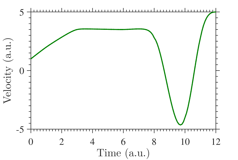
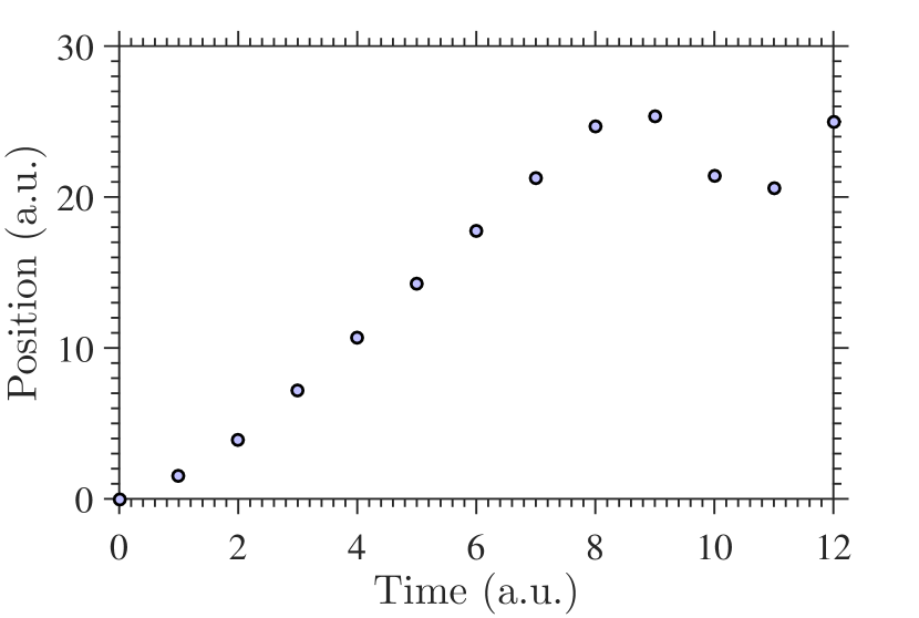
Figure 1: An example of solving a forward problem from a velocity curve (left) to calculate positions/distances (right). The velocity curve is the exponential cubic spline computed at $\vec{\xi}=[0,1,3,6,8,10,11,12]$. The positions were calculated from the velocity using the forward problem at $n=13$ different time instances. The time axis is given at arbitrary units (a.u.).

III The Bayesian Recipe

The inverse problem for the position-velocity scenario introduced in the previous section can be solved by means of Bayes’ rule,

$$p\left(\text{velocity}\in\mathbb{V}|\text{positions}\in\mathbb{U}\right)=\frac{p(\text{velocity}\in\mathbb{V})p(\text{positions}\in\mathbb{U}|\text{velocity}\in\mathbb{V})}{p(\text{positions}\in\mathbb{U})}$$ (III.1)

The relation depicted in Eq. (III.1) shows how the joint posterior probability distribution can be built to infer the velocity when the positions are given. Bayes’ rule in Eq. (III.1) can be rewritten using data and parameters given in Table 1 as follows,

$$p\left(\vec{f_{v}}\text{, }\vec{\lambda_{v}}\text{, }\vec{\xi_{v}}\text{, }E_{v}|\vec{t}\text{, }\vec{x}\text{, }I\right)=\frac{p(\vec{f_{v}}\text{, }\vec{\lambda_{v}}\text{, }\vec{\xi_{v}}\text{, }E_{v}|I)p(\vec{x}|\vec{f_{v}}\text{, }\vec{\lambda_{v}}\text{, }\vec{\xi_{v}}\text{, }E_{v}\text{, }\vec{t}\text{, }I)}{p(\vec{x}|I)}\text{,}$$ (III.2)

where the quantity $I$ represents all the relevant information that concerns the physical scenario under investigation together with the available knowledge about the experiment being performed. By assuming the independence in spline variables, the following relation is satisfied,

$$p(\vec{f_{v}},\vec{\lambda_{v}},\vec{\xi_{v}},E_{v}|I)=p\left(\vec{f_{v}}|I\right)p\left(\vec{\lambda_{v}}|I\right)p\left(\vec{\xi_{v}}|I\right)p\left(E_{v}|I\right)\text{.}$$ (III.3)

Substituting Eq. (III.3) into Eq. (III.2), we get

$$p \left(\vec{f_{v}}\text{, }\vec{\lambda_{v}}\text{, }\vec{\xi_{v}}\text{, }E_{v}|\vec{t}\text{, }\vec{x}\text{, }I\right)$$ (III.4)

$$= \frac{p\left(\vec{f_{v}}|I\right)p\left(\vec{\lambda_{v}}|I\right)p\left(\vec{\xi_{v}}|I\right)p\left(E_{v}|I\right)p(\vec{x}|\vec{f_{v}}\text{, }\vec{\lambda_{v}}\text{, }\vec{\xi_{v}}\text{, }E_{v}\text{, }\vec{t}\text{, }I)}{p(\vec{x}|I)}\text{.}$$

The evidence $p\left(\vec{x}|I\right)$ in Eq. (III.1) and (III.2) is given by,

$$p\left(\vec{x}|I\right)\overset{\text{def}}{=}$$ (III.5)

$$\iiiint p\left(\vec{f_{v}}|I\right)p\left(\vec{\lambda_{v}}|I\right)p\left(\vec{\xi_{v}}|I\right)p\left(E_{v}|I\right)p(\vec{x}|\vec{f_{v}}\text{, }\vec{\lambda_{v}}\text{, }\vec{\xi_{v}}\text{, }E_{v}\text{, }\vec{t}\text{, }I)d\vec{f_{v}}d\vec{\lambda_{v}}d\vec{\xi_{v}}dE_{v}\text{,}$$

where the likelihood distribution is given by $p(\vec{x}|\vec{f_{v}}$, $\vec{\lambda_{v}}$, $\vec{\xi_{v}}$, $E_{v}$, $\vec{t}$, $I)$. The likelihood distribution affirms the relation between the data and the spline values. Since the position data $x_{i}$ with $i=1$,…, $n$ is contaminated with noise, omitting the arrow notation for vectorial quantities, Eq. (II.7) can be rewritten including the noise term as,

$$x_{i}=\begin{cases}x_{1}+\sum_{\gamma=1}^{i-1}\int_{\xi_{v_{\gamma}}}^{\xi_{v_{\gamma+1}}}S_{v_{\gamma}}\left(t\text{, }f_{v}\text{, }\lambda_{v}\text{, }\xi_{v}\text{, }E_{v}\right)dt+\int_{\xi_{v_{i}}}^{t_{i}}S_{v_{i}}\left(t\text{, }f_{v}\text{, }\lambda_{v}\text{, }\xi_{v}\text{, }E_{v}\right)dt\\ +\epsilon_{i}\text{,}\quad\mbox{for }\xi_{v_{i}}<t_{i}<\xi_{v_{i+1}}\\ x_{1}+\sum_{\gamma=1}^{i-1}\int_{\xi_{v_{\gamma}}}^{\xi_{v_{\gamma}+1}}S_{v_{\gamma}}\left(t\text{, }f_{v}\text{, }\lambda_{v}\text{, }\xi_{v}\text{, }E_{v}\right)dt+\epsilon_{i}\text{,}\\ \quad\mbox{for }t_{i}=\xi_{v_{i}}\end{cases}\text{,}$$ (III.6)

where the noise vector $\vec{\epsilon}\overset{\text{def}}{\mathbf{=}}\left(\epsilon_{1}\text{,..., }\epsilon_{n}\right)$ is assumed to be linear and, in addition, is assumed to be Gaussian-distributed with

$$\vec{\epsilon}\sim N\left(\vec{\mu},\Sigma\right)\text{.}$$ (III.7)

In Eq. (III.7), the quantity $\vec{\mu}$ is the $\left(n\times 1\right)$-dimensional mean vector while $\Sigma$ is a $\left(n\times n\right)$-dimensional covariance matrix of the noise. Furthermore, the noise is assumed to be uncorrelated. In other words, $\Sigma$ is a diagonal matrix with diagonal elements given by $\left\{\sigma_{1}\text{,}\cdots\text{, }\sigma_{n}\right\}$. It is also assumed that $\vec{\mu}=\vec{0}$. From Eq. (III.6), the following equation can be written for the $i$-th noise term,

$$\epsilon_{i}=x_{i}-\left(x_{1}+\sum_{\gamma=1}^{i-1}\int_{\xi_{v_{\gamma}}}^{\xi_{v_{\gamma+1}}}S_{v_{\gamma}}\left(t\text{, }f_{v}\text{, }\lambda_{v}\text{, }\xi_{v}\text{, }E_{v}\right)dt+\int_{\xi_{v_{i}}}^{t_{i}}S_{v_{i}}\left(t\text{, }f_{v}\text{, }\lambda_{v}\text{, }\xi_{v}\text{, }E_{v}\right)dt\right)\text{,}\quad$$ (III.8)

where $i=1$,$\cdots$, $n$. The symbols $S_{v_{\gamma}}$ and $S_{v_{i}}$ denote the exponential spline function in Eq. (II.2) in the $\gamma^{th}$ and the $i^{th}$ sub-intervals, respectively.

Assuming that for all $i=1$,…, $n$ the data values are independent and identically distributed, the likelihood distribution can be rewritten as

$$p(\vec{x}|\vec{f_{v}}\text{, }\vec{\lambda_{v}}\text{, }\vec{\xi_{v}}\text{, }E_{v}\text{, }\vec{t}\text{, }I)=\prod_{i=1}^{n}p(x_{i}|\vec{f_{v}}\text{, }\vec{\lambda_{v}}\text{, }\vec{\xi_{v}}\text{, }E_{v}\text{, }t_{i}\text{, }I)\text{.}$$ (III.9)

Combining Eqs. (III.8) and (III.9) together with the additional assumption that $\sigma_{i}=\sigma_{e}=$constant for any $1\leq i\leq n$, the likelihood distribution becomes (case I of Eq. (III.6) is assumed here for generality),

$$p(\vec{x}|\vec{f_{v}}\text{, }\vec{\lambda_{v}}\text{, }\vec{\xi_{v}}\text{, }E_{v}\text{, }\vec{t}\text{, }I)=\prod_{i=1}^{n}\frac{1}{\sqrt{2\pi\sigma_{e}^{2}}}\exp\left[-\frac{1}{2\sigma_{e}^{2}}\left(\epsilon_{i}\right)^{2}\right]$$

$$=\left(2\pi\sigma_{e}^{2}\right)^{-n/2}\exp\sum_{i=1}^{n}\left\{-\frac{1}{2\sigma_{e}^{2}}\left[x_{i}-\left(x_{1}+\sum_{\gamma=1}^{i-1}\int_{\xi_{v_{\gamma}}}^{\xi_{v_{\gamma+1}}}S_{v_{\gamma}}(\cdot)dt+\int_{\xi_{v_{i}}}^{t_{i}}S_{v_{i}}(\cdot)dt\right)\right]^{2}\right\}$$

$$=\left(2\pi\sigma_{e}^{2}\right)^{-n/2}\exp\sum_{i=1}^{n}\mathcal{G}(x_{i}\text{,}\vec{\text{ }f_{v}}\text{,}\vec{\text{ }\lambda_{v}}\text{, }\vec{\xi_{v}}\text{, }E_{v}\text{, }\vec{t})\text{,}$$ (III.10)

with

$$\mathcal{G}(x_{i}\text{,}\vec{\text{ }f_{v}}\text{,}\vec{\text{ }\lambda_{v}}\text{, }\vec{\xi_{v}}\text{, }E_{v}\text{, }\vec{t})\overset{\text{def}}{=}-\frac{1}{2\sigma_{e}^{2}}\left[x_{i}-\left(x_{1}+\sum_{\gamma=1}^{i-1}\int_{\xi_{v_{\gamma}}}^{\xi_{v_{\gamma+1}}}S_{v_{\gamma}}(\cdot)dt+\int_{\xi_{v_{i}}}^{t_{i}}S_{v_{i}}(\cdot)dt\right)\right]^{2}\text{.}$$ (III.11)

When the number of knots is known ahead of time, the product of prior distributions in Eq. (III.3) can be rewritten as

$$p(\vec{f_{v}}\text{, }\vec{\lambda_{v}}\text{, }\vec{\xi_{v}}\text{, }E_{v}|I)=p\left(\vec{f_{v}}|E_{v}\text{, }I\right)p\left(\vec{\lambda_{v}}|E_{v}\text{, }I\right)p\left(\vec{\xi_{v}}|E_{v}\text{, }I\right)\text{.}$$ (III.12)

III.1 The choice of prior probability distributions

The shape of the curve produced between knots depends on the values of $\vec{\lambda}_{v}$. One of the concerns with the tension parameter is that it is a scale parameter and it can assume any real number. The shape of the curve between two knots can change from cubic function to a polygonal function when its value goes from $0$ to $\infty$ rentrop1980algorithm ; fischer2006flexible . A polygonal function is not a good representation of a moving object due to its lack of smoothness. Thus, the value of the tension plays a big role in getting the perfect velocity curve as explained by the observed data. Therefore, prior distributions on $\lambda_{v}$ should be chosen carefully to control its value.

Previous works in the literature fischer2006flexible ; fischer2006non has used Jeffreys’ prior to scale down large values produced for the tension. In this paper, we have employed a Gaussian distribution as a prior for the tension. It allows the choice of sensible values with a higher probability and non-sensible values with a lower probability. A bonus of choosing a Gaussian prior is that it is a conjugate prior of the Gaussian likelihood and, as a consequence, makes the resulting posterior a member of a family of the Gaussian distributions.

Assuming identical and independent tension parameters $\vec{\lambda_{v}}$, the prior distribution $p(\vec{\lambda_{v}}|E_{v}$, $I)$ in Eq. (III.12) can be written as

$$p(\vec{\lambda_{v}}|E_{v}\text{, }I) =\prod_{i=1}^{E_{v}-1}p\left(\lambda_{v_{i}}|E_{v}\text{, }I\right)$$

$$=\prod_{i=1}^{E_{v}-1}\frac{1}{\sqrt{2\pi\sigma_{\theta_{\lambda_{i}}}^{2}}}\exp\left[-\frac{\left(\lambda_{v_{i}}-\mu_{i}\right)^{2}}{2\sigma_{\theta_{\lambda_{i}}}^{2}}\right]$$

$$=\left(2\pi\sigma_{\theta_{\lambda}}^{2}\right)^{-(E_{v}-1)/2}\exp\left[-\sum_{i=1}^{E_{v}-1}\frac{\left(\lambda_{v_{i}}-\mu_{i}\right)^{2}}{2\sigma_{\theta_{\lambda}}^{2}}\right]$$ (III.13)

$$(\text{by taking }\sigma_{\theta_{\lambda_{i}}}=\sigma_{\theta_{\lambda}}\forall i\text{ with }1\leq i\leq E_{v}-1)\text{,}$$

with $\mu_{i}$ and $\sigma_{\theta_{\lambda}}$ representing the mean and the standard deviation of the parameter $\lambda_{v_{i}}$. The prior distributions $p\left(\vec{f_{v}}|E_{v}\text{, }I\right)$ and $p\left(\vec{\xi_{v}}|E_{v}\text{, }I\right)$ in Eq. (III.12) are assumed to be constant as no prior information on the behavior was identified. Finally, using Eqs. (III.10) and (III.1), the posterior distribution $p\left(\vec{f_{v}}\text{,}\vec{\text{ }\lambda_{v}}\text{, }\vec{\xi}\text{, }E_{v}|\vec{t}\text{, }\vec{x}\text{, }I\right)$ in Eq. (III.2) can be viewed as,

$$p\left(\vec{f_{v}}\text{,}\vec{\text{ }\lambda_{v}}\text{, }\vec{\xi}\text{, }E_{v}|\vec{t}\text{, }\vec{x}\text{, }I\right) \propto p\left(\vec{\lambda_{v}}|E_{v}\text{, }I\right)p(\vec{x}|\vec{f_{v}}\text{, }\vec{\lambda_{v}}\text{, }\vec{\xi}\text{, }E_{v}\text{, }\vec{t}\text{, }I)$$

$$\propto\left(2\pi\sigma_{\theta_{\lambda}}^{2}\right)^{-(E_{v}-1)/2+(-n/2)}$$ (III.14)

$$\exp\left[-\sum_{i=1}^{E_{v}-1}\frac{\left(\lambda_{v_{i}}-\mu_{i}\right)^{2}}{2\sigma_{\theta_{\lambda}}^{2}}+\sum_{i=1}^{n}\mathcal{G}\left(x_{i}\text{,}\vec{\text{ }f_{v}}\text{, }\vec{\lambda_{v}}\text{, }\vec{\xi}\text{, }E_{v}\text{, }\vec{t}\right)\right]$$

where $\mathcal{G}(x_{i}$,$\vec{\text{ }f_{v}}$,$\vec{\text{ }\lambda_{v}}$, $\vec{\xi_{v}}$, $E_{v}$, $\vec{t})$ is given in Eq. (III.11).

IV Methodology

Synthetic data of time-positions were generated from the same velocity curve used in the forward problem shown in Fig. 1, characterized by a reasonably large sample size with $n=121$. Then, the Gaussian noise with $\mu=0$ and $\sigma$ was added to the data,

$$x(t)=x_{\text{true}}(t)+\left[\mu+z\sigma\right]\text{,}$$ (IV.1)

with $z$ being the standard parameter introduced when dealing with normalized Gaussian data sets. Following from the posterior distributions defined in Section III, the number of parameters of the system is determined by $E_{v}$. Furthermore, when the positions and the number of knots are provided by the user, the total number of parameters of the system will be $2E_{v}-1$.

For the synthetic data, following the work in Ref. rentrop1980algorithm , we select $E_{v}=8$ knots at $\vec{\xi_{v}}=[0,1,3,6,8,10,11,12]$ in to inferring the spline. Then, the posterior distribution with different priors (see Eq.  (III)) were simulated using a hybrid MCMC algorithm called DRAM haario2006dram . The simulation begins with an initial minimization process of the negative of the posterior distributions. The initial values of the parameters used were,

$$f_{v_{\text{initial}}}=0\text{, and }\lambda_{v_{\text{initial}}}=0.001.$$ (IV.2)

We remark that the posterior distribution is undefined at $\lambda_{v}=0$ and, in addition, the smallest value that MATLAB MATLAB:2015 could handle for $\lambda_{v}$ was experimentally found to be equal to $0.001$. The initial minimization acts as a jump start to the DRAM algorithm. The proposal distributions of the parameters in DRAM that generate the candidate sample values are Gaussian distributions. The user must input values for the parameters of the proposal distributions (i.e., mean and variance of Gaussian distributions) as given in Table 2 with $LB$ and $UB$ being the lower and upper bounds of the parameters, respectively.

Table 2: Initial proposal distributions of the system parameters.

parameter proposal distribution prior distribution $f_{v_{i}}$ for $i=1,\cdots,E_{v}$ Gaussian($\mu_{v_{i}},\sigma_{v_{i}}^{2}$) $\in(LB_{v_{i}},UB_{v_{i}})$ $\mu_{\theta_{v_{i}}},\sigma_{\theta_{v_{i}}}$ $\lambda_{v_{i}}$ for $i=1,\cdots,E_{v}-1$ Gaussian($\mu_{\lambda_{i}},\sigma_{\lambda_{i}}^{2}$) $\in(LB_{\lambda_{i}},UB_{\lambda_{i}})$ $\mu_{\theta_{\lambda_{i}}},\sigma_{\theta_{\lambda_{i}}}$

The optimum values $\vec{f_{v}}^{\ast}$ and$\vec{\text{ }\lambda_{v}}^{\ast}$ determined by the initial minimization were used as the mean values of the proposal distributions, so that the initial proposal distributions are centered around $\vec{f_{v}}^{\ast}$ and$\vec{\text{ }\lambda_{v}}^{\ast}$. The information of prior distributions can be specified with prior means $\mu_{\theta_{v_{i}}}$, $\mu_{\theta_{\lambda_{i}}}$ and prior variances $\sigma_{\theta_{v_{i}}}$, $\sigma_{\theta_{\lambda_{i}}}$. The DRAM procedure takes the variance of the prior as the initial variance of the parameters if the covariance matrix is not specified by the user. When the prior variance is infinity, the variances of the proposal distributions are calculated as,

$$\sigma_{v_{i}}^{2}=\left(\mu_{v_{i}}\times 0.05\right)^{2}\text{, and }\sigma_{\lambda_{i}}^{2}=\left(\mu_{\lambda_{i}}\times 0.05\right)^{2}\text{.}$$ (IV.3)

In other words, if no prior information is available about the parameter, $5\%$ of the mean of the initial distribution is taken as the initial variance. Finally, samples were drawn from these Gaussian proposals and the marginal densities of the parameters were computed. The MCMC simulations were run until convergence was observed. Each sampling procedure of length $\mathrm{MCMCnsimu}$ was repeated $\mathrm{MCMCN}=100$ times. At each of the $\mathrm{MCMCN}$-th repetitions, the random noise with the same mean and the same standard deviation as reported in Eq. (IV.1) was added. Hence, a different set of data with the same level of noise was used at each iteration. At each $\mathrm{MCMCN}$-th repetition, the initial minimization process was newly ran. All the sample chains were stored and, in addition, the first few samples were destroyed using a $\mathrm{MCMCnsimu}\ast p\%$ burn-in period. The quantity $p$ denotes the burn-in time parameter and, in our case is specified by the interval $(0,100)$. The average marginal densities were then computed for each parameter using the remaining samples. In what follows, we assume that nsimu denotes the remaining number of samples after burn-in period, that is, $\mathrm{nsimu}\overset{\text{def}}{=}(1-p)\%\ast\mathrm{MCMCnsimu}$. Then, for any $k=1$,$\cdots$, $E_{v}$, the mean values $\left\{f_{v_{k}}^{\ast}\right\}$ of those mean marginal densities were calculated as,

$$f_{v_{k}}^{\ast}\overset{\text{def}}{=}\frac{1}{\mathrm{nsimu}}\sum_{i=1}^{\mathrm{nsimu}}\overline{f_{v}}_{ki}\text{,}$$ (IV.4)

where$\overline{\text{ }f_{v}}_{ki}$ denote the average sample values of $f_{v_{k}}$ after MCMCN number of iterations,

$$\overline{f_{v}}_{ki}\overset{\text{def}}{=}\frac{1}{\mathrm{MCMCN}}\sum_{j=1}^{\mathrm{MCMCN}}f_{v_{kij}}\text{.}$$ (IV.5)

Following the same line of reasoning presented for Eqs. (IV.4) and (IV.5), we also have

$$\lambda_{v_{s}}^{\ast}\overset{\text{def}}{=}\frac{1}{\mathrm{nsimu}}\sum_{i=1}^{\mathrm{nsimu}}\overline{\lambda_{v}}_{si}=\frac{1}{\mathrm{nsimu}\times\mathrm{MCMCN}}\sum_{i=1}^{\mathrm{nsimu}}\sum_{j=1}^{\mathrm{MCMCN}}\lambda_{v_{sij}}\text{,}$$ (IV.6)

for any $s=1$,$\cdots$, $E_{v}-1$ with $\overline{\lambda_{v}}_{si}$ denoting the average sample values of tension after MCMCN number of iterations,

$$\overline{\lambda_{v}}_{si}\overset{\text{def}}{=}\frac{1}{\mathrm{MCMCN}}\sum_{j=1}^{\mathrm{MCMCN}}\lambda_{v_{sij}}\text{.}$$ (IV.7)

Finally, the standard deviations $\left\{\sigma_{v_{k}}^{\ast}\right\}$ and $\left\{\sigma_{\lambda_{s}}^{\ast}\right\}$ of the parameters are calculated from the average of all chains after MCMCN iterations as,

$$\sigma_{v_{k}}^{\ast}\overset{\text{def}}{=}\sqrt{\frac{1}{\mathrm{nsimu}-1}\sum_{i=1}^{\mathrm{nsimu}}\left(\overline{f_{v}}_{ki}-f_{v_{k}}^{\ast}\right)^{2}}\text{,}$$ (IV.8)

for any $k=1$,$\cdots$, $E_{v}$ and,

$$\sigma_{\lambda_{s}}^{\ast}\overset{\text{def}}{=}\sqrt{\frac{1}{\mathrm{nsimu}-1}\sum_{i=1}^{\mathrm{nsimu}}\left(\overline{\lambda}_{v_{si}}-\lambda_{v_{s}}^{\ast}\right)^{2}}\text{,}$$ (IV.9)

for any $s=1$,$\cdots$, $E_{v}-1$, respectively.

V Results

This section presents the results obtained from the method explained in the previous sections. The sensitivity of gradient estimates on the noise levels of the position data are tested. The noise levels on x-space is depicted in Fig. 1 with different noise levels are denoted by $\sigma_{e}$. The noise of same level was added randomly at the beginning of the optimization process with keeping all other variables same: The data size $n$, the number of knots of the exponential cubic spline $E_{v}$, the positions of the knots $\vec{\xi_{v}}$, the number of MCMC iterations $\mathrm{MCMCN}$, and the true data positions. The added noise have five different levels of $\sigma_{e}\in\left\{0.001\text{, }0.3\text{, }0.7\text{, }1.0\text{, }1.3\right\}$ from a standard Gaussian distribution. By the definition of the Gaussian distribution, the first four noise levels have a probability of $68.2\%$ while the last noise level has a probability of $95\%$.The noise levels are selected so that that they represent distinct possibilities of the Gaussian noise.

The sensitivity of noise levels was investigated for the posterior distribution with the Gaussian prior used for the tension parameter. These results of the sensitivity analysis were compared against a common traditional method of fitting the same type of exponential cubic spline in $\mathbb{U}$ and the gradient is obtained by analytically differentiating the resulting fitted spline function. The notation “$i$-fit ($i$-space) with $i=$ x, v” denotes the fact that the $i$-fit was fitted on the $i$-space where the x-fit is the distance profile while the v-fit is the gradient profile.

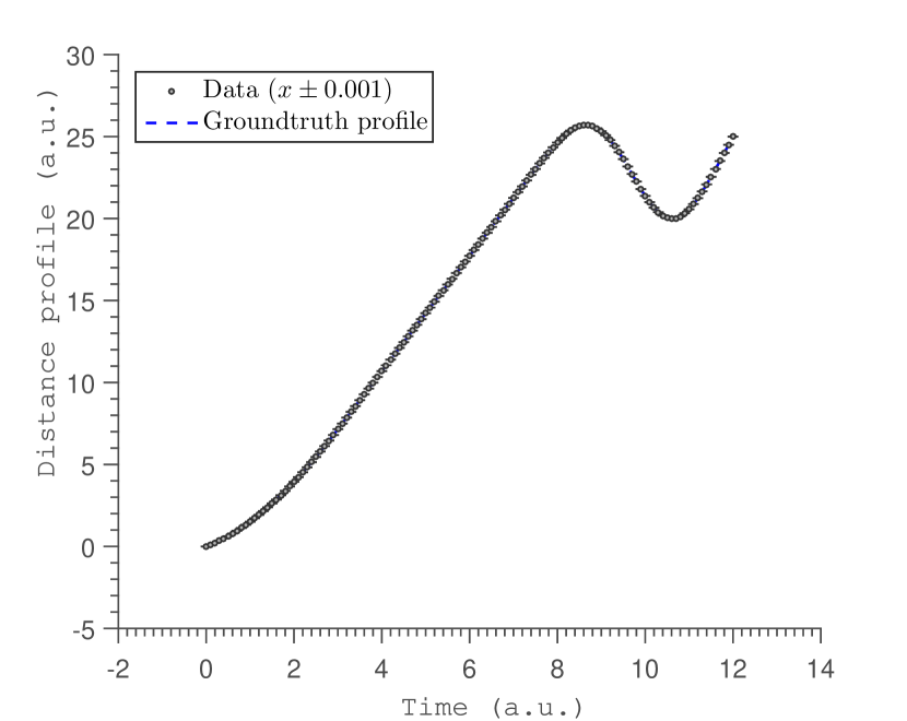
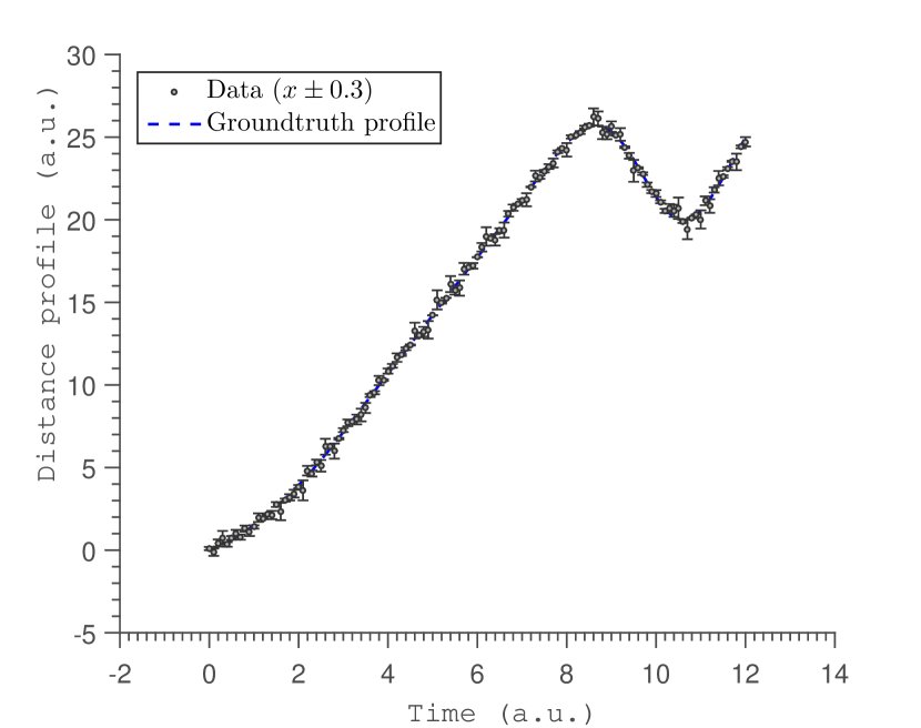
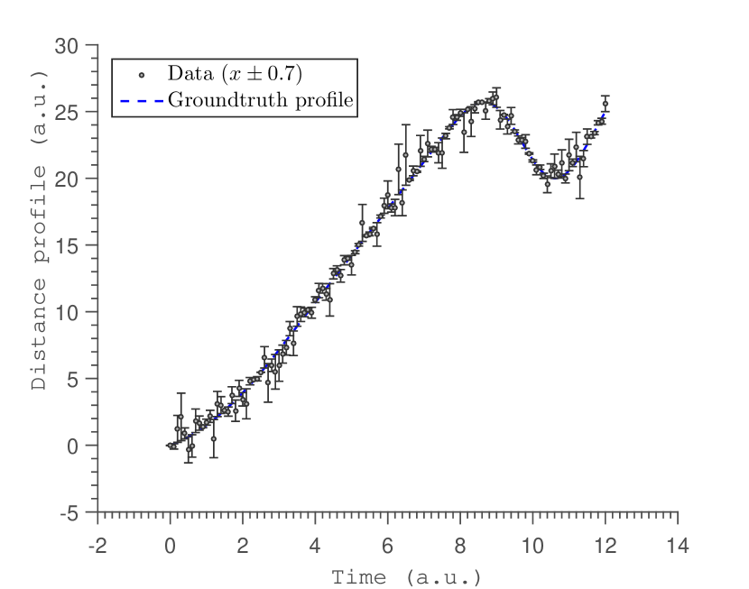
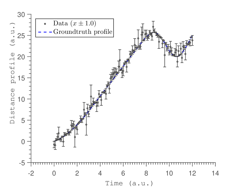
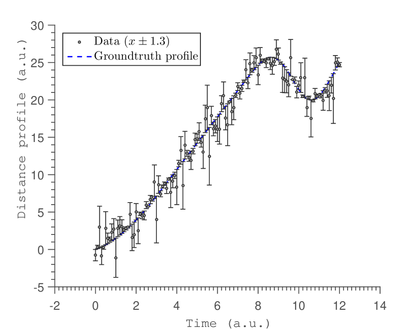
Figure 2: The panel of time-position data with error bars at five different noise levels. Noise levels increase from left to right and top to bottom. The length of error bars is relative to the magnitude of the noise.

A constant force is observed between the times $0-8(a.u.)$ and short impulses are observed between the times $8-11(a.u.)$. Moreover, it is observed that as the noise level increases, the data around the short impulses tends to get fuzzier so that it is hard to identify the trajectory. The marginalized posterior distributions for each parameter is simulated using MCMC sampling. When the noise increases, the width of the marginal distributions were expanded. This, in turn, resulted in an increased length of the error bars of the parameter estimates. The marginal probability distribution of $f_{v_{1}}$ is shown in Fig. 3. These uncertainties of the $f_{v_{i}}$ parameters are shown as error bars in Fig. 4 (left panel) and as Bayesian credible intervals in Fig. 4 (right panel). The gradient estimate is obtained at all noise levels by placing the model in $\mathbb{V}$ and is shown in Fig. 4. The estimates almost overlap with the ground truth data at all noise levels, except at the boundaries and around the time $t=10a.u.$, where the short impulses were present in the position profile.

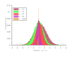
Figure 3: The comparison of marginal probability densities of $f_{v_{1}}$ parameter at all noise levels.

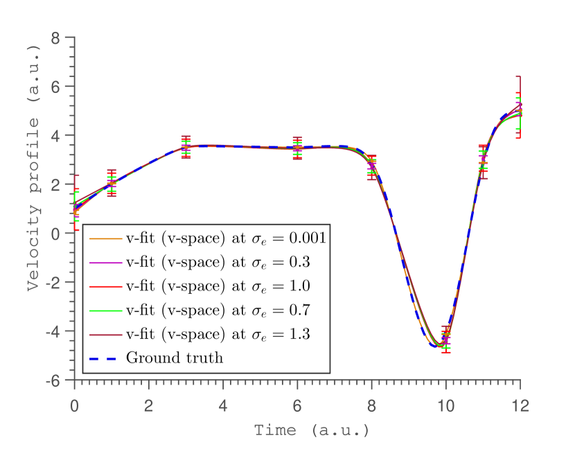
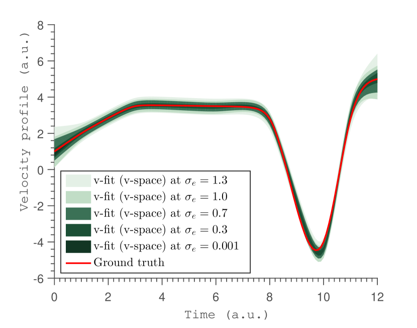
Figure 4: The gradient estimates obtained at the five different noise levels. The uncertainty of the velocity estimates ($\hat{\sigma}_{v}$) are shown using error bars (left panel) and credible intervals (right panel).

The uncertainties of both velocity and tension parameters are characterized in Fig. 5. The uncertainty of the velocity parameters with the noise level exhibits a linear relationship reflecting the linear relationship of velocity parameters in the likelihood function. The uncertainty of the tension parameters does not show any specific pattern as it has a non linear pattern in the likelihood.

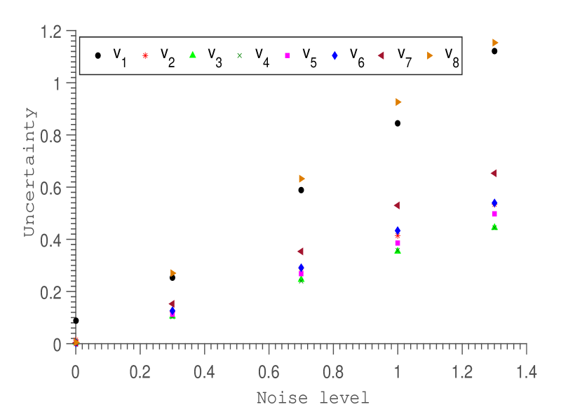
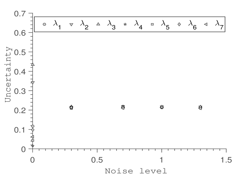
Figure 5: The relationship between uncertainty of the estimates and the noise level of the system. The left panel depicts the relationship of velocity parameters whereas the right panel shows the relationship of tension parameters.

The gradient estimates are compared with the analytic derivative of the x-fit obtained in $\mathbb{U}$. The x-fit is obtained by fitting the same exponential cubic spline to the time-position data in $\mathbb{U}$. This was performed at the same knot positions. The gradient profile, the acceleration profile, and position profile were obtained from the two methods (via v-fit from $\mathbb{V}$ and x-fit from $\mathbb{U}$) and compared in Fig. 6, Fig. 7 and Fig. 8, respectively. The two types of estimates of acceleration profile from the v-space and the x-space were obtained by differentiating the v-fit (v-space) and by finite differencing the v-fit (x-space), respectively, from Fig. 6.

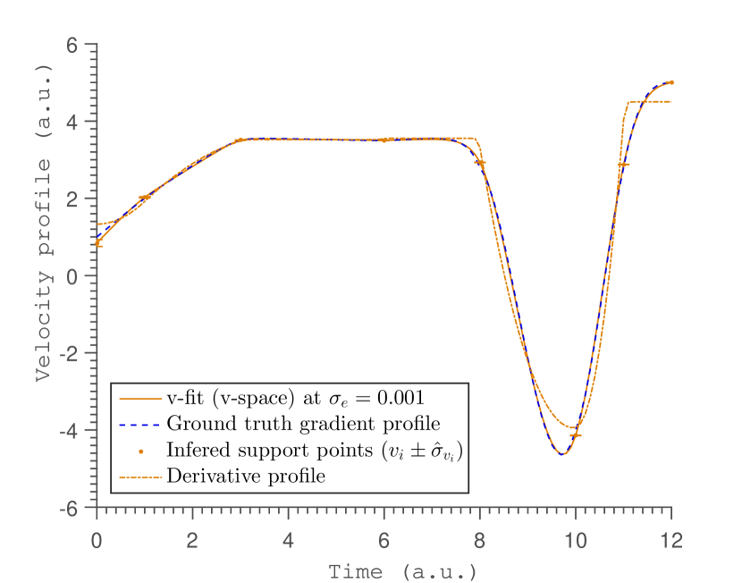
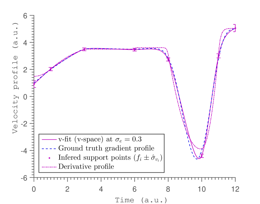
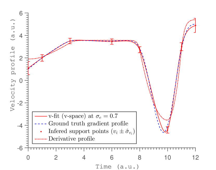
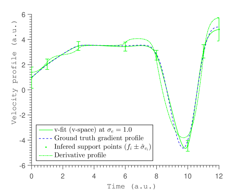
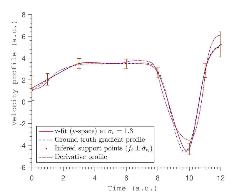
Figure 6: The panel of velocity estimates from the two spaces compared at five different noise levels. The noise level increases from left to right and top to bottom.

The gradient estimates that emerge from the two spaces (namely, the x-space and v-space) clearly show some remarkable differences. In particular, the difference in accuracy is shown in Table 3 using the error norm,

$$||e||^{2}\overset{\text{def}}{=}\sum_{i=1}^{L}\left(f_{v_{\text{estimated}_{i}}}-f_{v_{\text{true}_{i}}}\right)^{2}\text{,}$$ (V.1)

where $L$ is the sample size hansen1992analysis .

Table 3: The comparison of accuracy of velocity fit from v space, and x space.

$||e||^{2}$ noise level v-fit Derivative of x-fit $0.001$ $0.2077$ $14.4107$ $0.3$ $1.9679$ $15.0792$ $0.7$ $3.1793$ $20.9974$ $1$ $3.1569$ $30.1122$ $1.3$ $3.8159$ $31.2719$

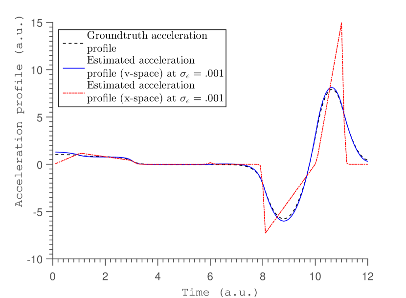
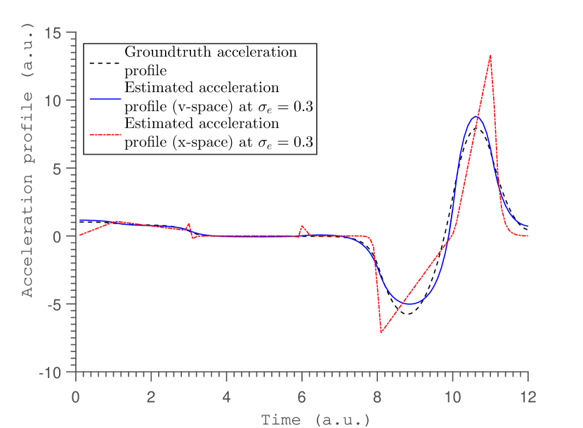
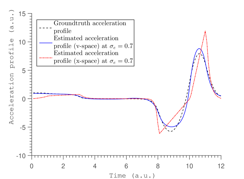
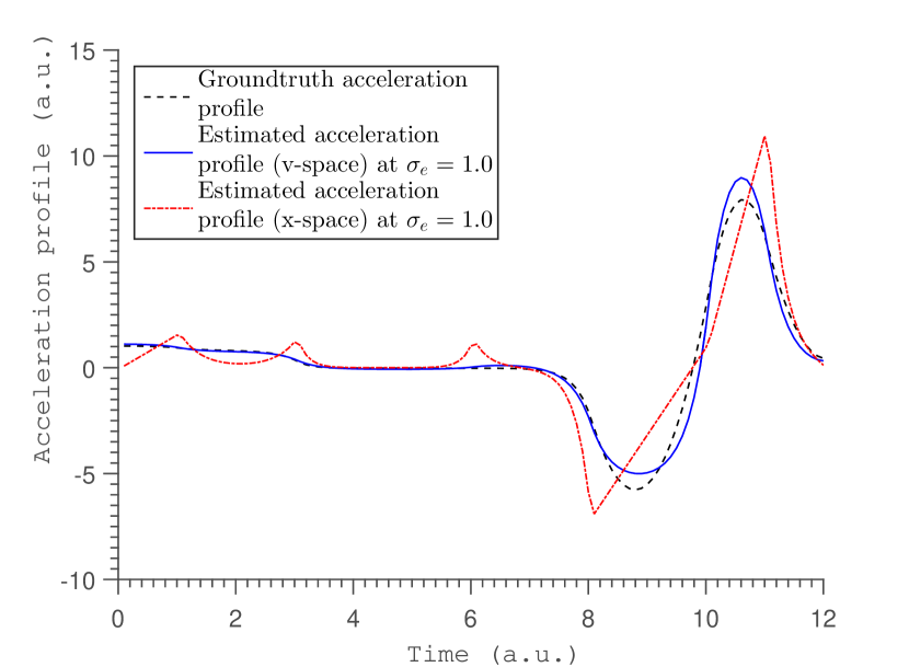
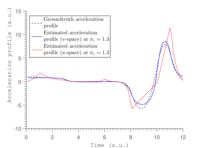
Figure 7: The panel of acceleration estimates obtained from two methods are compared at five different noise levels.

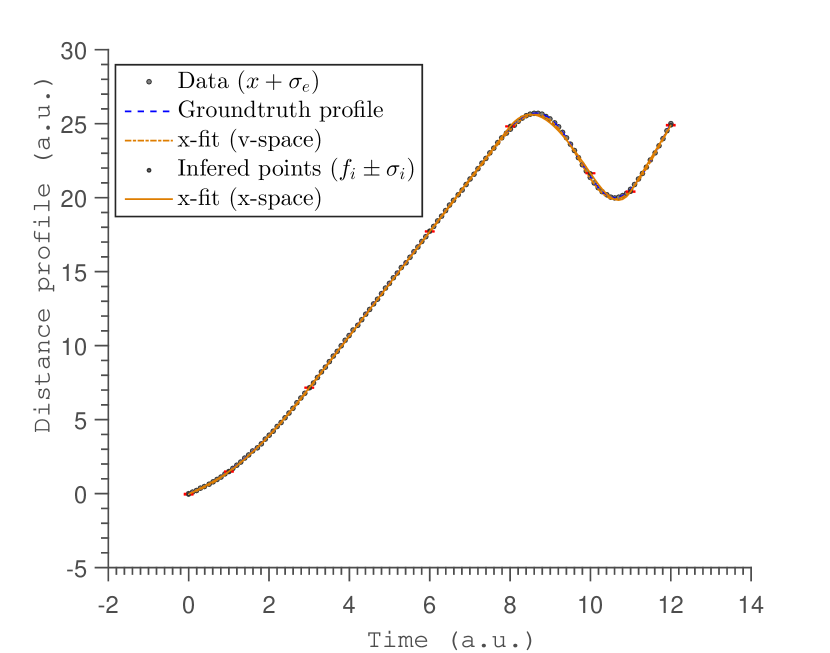
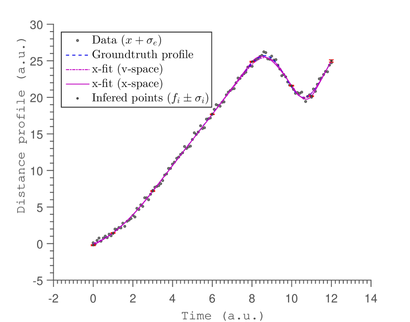
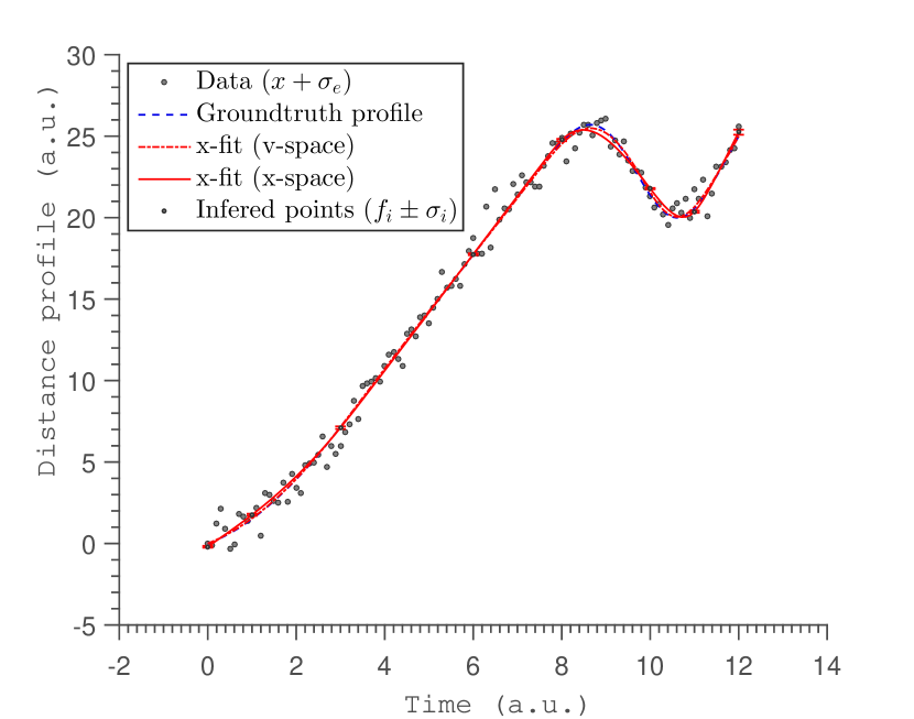
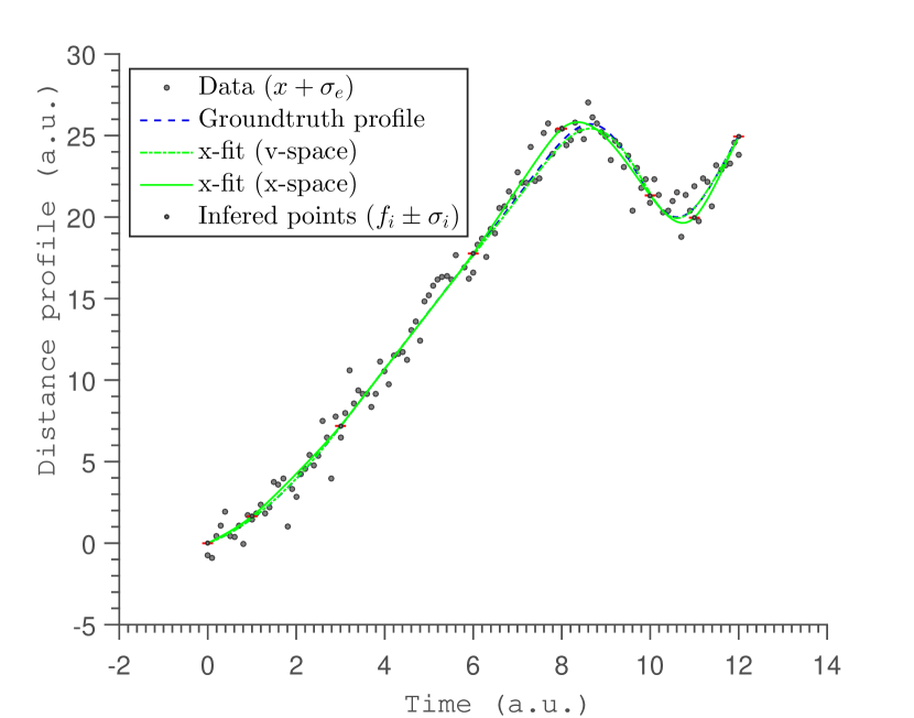
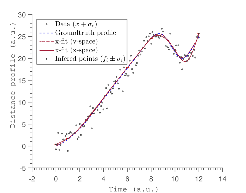
Figure 8: The panel of x-fit estimates obtained from two different spaces compared at five different noise levels.

The acceleration characterizes the acting forces on the object. The acceleration estimate (x-space) could not achieve constant force where it is expected. The errors at short impulses around $t=10$ a.u. started getting very large and this indicates the possibility of infinite forces. Moreover, the acceleration profile from the x-space (red dashed-dot lines) is not realistic with its very sharp turns. Therefore, the acceleration estimate from the velocity space is a reliable estimator of acting forces. The goodness of the fit is tested by studying the error sum of squares (SSE) defined as merriman1909text ,

$$\mathrm{SSE}\overset{\text{def}}{=}\sum_{i=1}^{n}\left(\hat{f}_{i}-f_{i}\right)^{2}$$ (V.2)

where $\hat{f}_{i}$ represent the estimated function values. The quantity $f_{i}$ in Eq.  (V.2) is replaced with noisy $f_{i}$ to obtain the second and the third columns in Table 4 while $f_{i}$ is replaced with the original $f_{i}$ without noise to calculate the fourth and fifth columns in the same table. The trajectory estimate is a bonus product from the gradient profile (v-space) and is obtained by integrating the gradient estimate (v-space). The trajectory estimates (position profiles) are compared in Fig. 8. The x-fit (x-space) follows the noisy data closely. This is because when fitting a curve in the same space as data, that curve is trying to minimize the SSE which means it tries to match the data as much as possible. Therefore, the x-fit from $\mathbb{U}$ tries to satisfy the noisy data as much as possible.  However, the x-fit (v-space) follows the ground truth data more than it follows the noisy data. When integrating the v-fit (v-space), an additional order of differentiability is added to the trajectory estimate. Therefore, the x-fit (v-space) has a higher order of differentiability than that of the x-fit (x-space). This additional order of differentiability ensures the continuity of the velocity and, therefore, it satisfies the constraint of the finite force of the object.

Table 4: The comparison of the quality of x-fit from x and v spaces respectively using error sum of squares (SSE).

SSE with noisy data SSE with true data $\sigma_{e}$ x-fit ($\mathbb{U}$) x-fit ($\mathbb{V}$) x-fit ($\mathbb{U}$) x-fit ($\mathbb{V}$) $0.001$ $1.1743$ $0.6082$ $1.1753$ $0.6089$ $0.3$ $12.4677$ $12.6049$ $2.1946$ $0.8541$ $0.7$ $62.4582$ $63.4059$ $4.1855$ $0.8176$ $1.0$ $121.0864$ $120.8161$ $13.3478$ $1.1253$ $1.3$ $163.1339$ $264.3176$ $18.9582$ $3.1651$

The calculated squared sum of errors (SSE) with true data and noisy data are shown in the Table 4. The SSE values for noisy data are smaller for the x-fit (x-space). This, in turn, reflects the fact that the x-fit (x-space) follows noisy data better. However, the SSE values for true data are smaller for the x-fit (v-space). This fact, instead, reflects the fact that the x-fit (v-space) follows true data better.

VI Conclusion

In this paper, we proposed a method to compute the profile gradient of a noisy system using Bayesian inference strategy. The Bayesian inference method allowed the inference of an un-observable quantity, the gradient (velocity), by building a meaningful relationship between the un-observable gradient profile in one space (that is, the velocity space) and the observable data profile in another space (that is, the data space - $\mathbb{U}$). Furthermore, the gradient profile was modeled by the exponential cubic spline. The results of this new method are compared against a common method of fitting an exponential cubic spline in data space ($\mathbb{U}$) and taking the subsequent analytic derivative. The fitting in $\mathbb{U}$ was also performed in a Bayesian framework and the same DRAM sampler was used to simulate the posterior distributions. The results show that the gradient estimates obtained by modeling in v-space produce more accurate estimates than the results of the traditional method (see Table III). Moreover, it was able to produce better acceleration estimates with reliable and accurate values where a constant force is expected (see FIG. 7). The third type of estimate, the trajectory profile was also compared. We conclude that the x-fit estimates follow noisy data when solved by placing the model in the x-space while the x-fit estimates follows the ground truth data when solved placing the model in the velocity space (see FIG. 8 and Table IV). It is argued that by integrating the model in velocity space, an extra order of differentiability is added to x-fit ensuring the finite force constraint of a moving object.

In conclusion, the method demonstrated in this paper is a superior method to estimate the velocity of a moving object under finite force as compared to others in literature (for instance, see von2011digital and references therein). It ensured better estimates in all three cases: trajectory, velocity, and the acceleration.

We point out that although our main focus in this paper is on the proposal of a novel theoretical method to estimate a profile gradient from discrete noisy data, a number of improvements can be sought in its practical implementation. For instance, the use of an MCMC algorithm gains precision at the expense of speed. A faster algorithm (such as the Expectation Maximization algorithm dempster77 ) may be needed for real time estimation. Furthermore, the amount and placement of the knots lacks a systematic guiding principle. In the future we plan to use Bayesian model selection for determining the amount. For the placement issue, we can adopt a hierarchical approach by including spline knot location algorithms montoya14 in conjunction with our main algorithm. This would provide estimates for the values associated with the knots and where they should be located as well. Finally, we hope to apply our Bayesian estimation technique to more realistic problems where acceleration, velocity, and trajectory estimations are needed.

The authors would like to thank the meaningful and helpful discussions had with Udo Von Toussaint at the Max-Planck Institute in Garching, Germany.

Appendix A

In this Appendix, we present some details on the integration of the exponential cubic spline. The integration is done in two cases. In one case, one integrates the spline function between two knots and it is referred to as $I_{\text{full}}$. In the other case, one integrates the spline function from a knot to a random point before the next knot and it is referred to as $I_{\text{partial}}$. The two types of integrals yield,

$$I_{\text{full}}=\int_{\xi_{v_{k}}}^{\xi_{v_{k+1}}}S_{v}\left(t\text{, }f_{v}\text{, }\lambda_{v}\text{, }\xi_{v}\text{, }E_{v}\right)dt\text{,}$$ (A.1)

with $k=1$,$\cdots$, $E_{v}-1$, and

$$I_{\text{partial}}=\int_{\xi_{v_{k}}}^{t_{i}}S_{v}\left(t\text{, }f_{v}\text{, }\lambda_{v}\text{, }\xi_{v}\text{, }E_{v}\right)dt$$ (A.2)

with $k=1$,$\cdots$, $E_{v}-1$,$\,\ i=1$,$\cdots$, $n$, and $\xi_{v_{k}}\leq t_{i}<\xi_{v_{k+1}}$, respectively. The solutions to these two cases presented in Eq. (A.1) and Eq. (A.2) can be found analytically and result in the following expressions,

$$I_{\text{partial}} =\frac{f_{v_{i+1}}}{2h_{v_{i}}}(t_{i}-\xi_{v_{i}})^{2}+\frac{f_{v_{i}}(t_{i}-\xi_{v_{i}})}{2h_{v_{i}}}(2\xi_{v_{i+1}}-t_{i}-\xi_{v_{i}})$$ (A.3)

$$-\frac{M_{v_{i}}(t_{i}-\xi_{v_{i}})}{2\lambda_{v_{i}}^{2}h_{v_{i}}}(2\xi_{v_{i+1}}-t_{i}-\xi_{v_{i}})$$

$$+\frac{M_{v_{i}}}{\lambda_{v_{i}}^{3}\sinh(\lambda_{v_{i}}h_{v_{i}})}\left\{\cosh(\lambda_{v_{i}}h_{v_{i}})-\cosh\left[\lambda_{v_{i}}(t_{i}-\xi_{v_{i+1}})\right]\right\}$$

$$+\frac{M_{v_{i+1}}}{\lambda_{v_{i}}^{3}\sinh(\lambda_{v_{i}}h_{v_{i}})}\left\{\cosh\left[\lambda_{v_{i}}(t_{i}-\xi_{v_{i}})\right]-1\right\}-\frac{M_{v_{i+1}}}{2\lambda_{v_{i}}^{2}h_{v_{i}}}(t_{i}-\xi_{v_{i}})^{2}\text{,}$$ (A.4)

and,

$$I_{\text{full}}=\frac{f_{v_{i}}h_{v_{i}}}{2}+\frac{f_{v_{i+1}}h_{v_{i}}}{2}-\frac{M_{v_{i}}h_{v_{i}}}{2\lambda_{v_{i}}^{2}}-\frac{M_{v_{i+1}}h_{v_{i}}}{2\lambda_{v_{i}}^{2}}+\frac{(M_{v_{i+1}}+M_{v_{i}})}{\lambda_{v_{i}}^{3}}\tanh\left(\frac{\lambda_{v_{i}}h_{v_{i}}}{2}\right)\text{.}$$ (A.5)

Appendix B

In this Appendix, being in the framework of Markov chain Monte Carlo (MCMC) methods, we present some details on the Delayed Rejection Adaptive Metropolis (DRAM) algorithm used to compute posterior distributions in our work. DRAM is a hybrid algorithm where the concepts of Delayed Rejection (DR) and Adaptive Metropolis (AM) are combined for enhancing the performance of the Metropolis-Hastings (MH) type MCMC algorithms haario2006dram . In the basic MH algorithm, upon the rejection of the new candidate at a (j + 1)th state, the sample remains at the current point (j). However, when the Delayed Rejection is introduced, upon rejection, another new candidate z is drawn. Then, one finds out whether it can be accepted. The AM feature, instead, is a global adaptive strategy which is combined with the partial local adaptation caused by the DR strategy. The idea of AM is to tune the proposal distribution at each time step depending on the past. In other words, the covariance matrix of the proposal distribution depends on the history of the sample chain (sequence of samples). Usually the adaptation starts after an initial period of time (0, t).

Algorithm 1 DRAM

1:  for $j=1:N$ do

2:     Generate $y$ from $q\left(\Theta^{(j)},.\right)$ and $u$ from $U(0,1)$

3:     if $y$ is outside $\left(L,U\right)$ then

4:        Reject $y$ (level 1)

5:     else

6:        Calculate $\alpha_{1}(\Theta^{(j)},y)$

7:        if $u\leq\alpha_{1}(\Theta^{(j)},y)$ then

8:           $\Theta^{(j+1)}=y$

9:        else

10:           Reject $y$ (level 2) {starts delayed rejection}

11:           Generate new candidate $z$ from $q\left(y,.\right)$

12:           if $z$ is outside $\left(L,U\right)$ then

13:              Reject $z$ (level 3)

14:           else

15:              Calculate $\alpha_{2}(\Theta^{(j)},y,z)$ and $u$ from $U(0,1)$

16:              if $u\leq\alpha_{2}(\Theta^{(j)},y,z)$ then

17:                 $\Theta^{(j+1)}=z$

18:              else

19:                 Reject $z$ (level 4)

20:                 $\Theta^{(j+1)}=\Theta^{(j)}$

21:              end if

22:           end if

23:        end if

24:     end if

25:  end for

26:  Return the values $\{\Theta^{\left(0\right)},\Theta^{\left(1\right)},\Theta^{\left(2\right)},\cdots,\Theta^{\left(N\right)}\}$.

The basic steps of the DRAM algorithm is given in Algorithm 1 with an arbitrary initial point $\Theta^{(0)}$. The acceptance probabilities at steps 6 and 15 are shown in Eqs. (B.1a) and (B.1b) respectively.

$$\alpha_{1}\left(x,y\right) =\begin{cases}\mbox{min}\left[\frac{\pi\left(y\right)q\left(y,x\right)}{\pi\left(x\right)q\left(x,y\right)},1\right]\quad&\mbox{if }\pi\left(x\right)q\left(x,y\right)>0,\\ 1\quad&\mbox{otherwise}.\end{cases}$$ (B.1a)

$$\alpha_{2}\left(x,y,z\right) =\begin{cases}&\mbox{min}\left[\frac{\pi\left(z\right)}{\pi\left(x\right)}\frac{q\left(z,y\right)}{q\left(x,y\right)}\frac{q\left(z,y,x\right)}{q\left(x,y,z\right)}\frac{[1-\alpha_{1}\left(z,y\right)]}{[1-\alpha_{1}\left(x,y\right)]},1\right]\\ &\mbox{if }\pi\left(x\right)q\left(x,y\right)q\left(x,y,z\right)[1-\alpha_{1}\left(x,y\right)]>0,\\ 1&\quad\mbox{otherwise}.\end{cases}$$ (B.1b)

$q(\theta)$ represents the proposal distribution and $\Theta^{(j)}$ represents the set of parameters of the proposal distribution at j-th iteration.

References

- (1) U. von Toussaint and S. Gori, Digital particle image velocimetry using splines in tension, AIP Conf. Proc. 1305, 337 (2011).
- (2) Y. Feng, J. Goree, and B. Liu, Errors in particle tracking velocimetry with high-speed cameras, Review of Scientific Instruments 82, 053707 (2011).
- (3) M. A. Chilenski, M. Greenwald, Y. Marzouk, N. T. Howard, A. E. White, J. E. Rice, and J. R. Walk, Improved profile fitting and quantification of uncertainty in experimental measurements of impurity transport coefficients using Gaussian process regression, Nuclear Fusion 55, 023012 (2015).
- (4) R. H. Brown, S. C. Schneider, and M. G. Mulligan, Analysis of algorithms for velocity estimation from discrete position versus time data, IEEE Transactions on Industrial Electronics 39, 11 (1992).
- (5) C. H. Reinsch, Smoothing by spline functions, Numerische Mathematik 10, 177 (1967).
- (6) C. H. Reinsch, Smoothing by spline functions. II, Numerische Mathematik 16, 451 (1971).
- (7) T. J. Hastie and R. J. Tibshirani, Generalized additive models, Monographs on Statistics and Applied Probability, vol. 43 (1990).
- (8) G. Wahba, Spline models for observational data, SIAM, vol. 59 (1990).
- (9) M. P Wand and M. C. Jones, Kernel Smoothing, CRC Press (1994).
- (10) P. J. Green and B. W. Silverman, Nonparametric Regression and Generalized Linear Models: A Roughness Penalty Approach, CRC Press (1993).
- (11) S. Wold, Spline functions in data analysis, Technometrics 16, 1 (1974).
- (12) B. W. Silverman, Some aspects of the spline smoothing approach to non-parametric regression curve fitting, Journal of the Royal Statistical Society B47, 1 (1985).
- (13) G. Wahba, Improper priors, spline smoothing and the problem of guarding against model errors in regression, Journal of the Royal Statistical Society B40, 364 (1978).
- (14) G. S. Kimeldorf and G. Wahba, A correspondence between Bayesian estimation on stochastic processes and smoothing by splines, The Annals of Mathematical Statistics 41, 495 (1970).
- (15) C. F. Ansley and R. Kohn, Estimation, filtering, and smoothing in state space models with incompletely specified initial conditions, The Annals of Statistics 13, 1286 (1985).
- (16) S. M. Berry, R. J. Carroll, and D. Ruppert, Bayesian smoothing and regression splines for measurement error problems, Journal of the American Statistical Association 97, 160 (2002).
- (17) R. Fischer, K. M. Hanson, V. Dose, and W. von Der Linden, Background estimation in experimental spectra, Phys. Rev. E61, 1152 (2000).
- (18) V. Dose and R. Fischer, Function estimation employing exponential splines, AIP Conf. Proc. 803, 67 (2005).
- (19) R. Fischer and V. Dose, Flexible and reliable profile estimation using exponential splines, AIP Conf. Proc. 872, 296 (2006).
- (20) T. Bayes, An Essay towards Solving a Problem in the Doctrine of Chances. By the Late Rev. Mr. Bayes, F. R. S. Communicated by Mr. Price, in a Letter to John Canton, A. M. F. R. S, Philosophical Transactions of the Royal Society of London 53, 370 (1763).
- (21) G. E. P. Box and G. C. Tiao, Bayesian Inference in Statistical Analysis, vol. 40, John Wiley & Sons (2011).
- (22) J. Geweke, Bayesian inference in econometric models using Monte Carlo integration, Econometrica 57, 1317 (1989).
- (23) A. P. Dempster, A generalization of Bayesian inference, Journal of the Royal Statistical Society B30, 205 (1968).
- (24) D. Gamerman and H. F. Lopes, Markov Chain Monte Carlo: Stochastic Simulation for Bayesian Inference, CRC Press, 2006.
- (25) D. C. Knill and W. Richards, Perception as Bayesian Inference, Cambridge University Press (1996).
- (26) M. A. Newton and A. E. Raftery, Approximate Bayesian inference with the weighted likelihood bootstrap, Journal of the Royal Statistical Society B56, 3 (1994).
- (27) P Rentrop, An algorithm for the computation of the exponential spline, Numerische Mathematik 35, 81 (1980).
- (28) A. Mohammad-Djafari, Bayesian inference for inverse problems, AIP Conf. Proc. 617, 477 (2002).
- (29) D. Sivia and J. Skilling, Data Analysis: A Bayesian Tutorial, Oxford University Press (2006).
- (30) A. Gelman, J. B. Carlin, H. S. Stern, and D. B. Rubin, Bayesian Data Analysis, vol. 2, Taylor & Francis (2014).
- (31) R. Fischer, A. Dinklage, and Y. Turkin, Non-parametric profile gradient estimation, in the 33rd EPS Conference on Plasma Phys. Rome, 19 - 23 June 2006 ECA Vol. 30I, P-2.127 (2006).
- (32) H. Haario, M. Laine, A. Mira, and E. Saksman, DRAM: Efficient adaptive MCMC, Statistics and Computing 16, 339 (2006).
- (33) MATLAB, version R2015b, The MathWorks Inc. (2015).
- (34) P. C. Hansen, Analysis of discrete ill-posed problems by means of the L-curve, SIAM Review 34, 561 (1992).
- (35) M. Merriman, A text book on the Method of Least Squares, John Wiley & Sons (1909).
- (36) A. P. Dempster, N. M. Laird, and D. B. Rubin, Maximum likelihood from incomplete data via the EM algorithm, Journal of the Royal Statistical Society, Series B39 (Methodological), 1-38 (1977).
- (37) E. L. Montoya, N. Ulloa, and V. Miller, A simulation study comparing knot selection methods with equally spaced knots in a penalized regression spline, Int. J. Statistics and Probability 3, 96 (2014).