Particle Event Generator: A Simple-in-Use System PEGASUS version 1.0

¹Skobeltsyn Institute of Nuclear Physics, Lomonosov Moscow State University, 119991, Moscow, Russia
²Joint Institute for Nuclear Research, 141980, Dubna, Moscow region, Russia
³P.N. Lebedev Physics Institute, 119991 Moscow, Russia

Abstract

pegasus is a parton-level Monte-Carlo event generator designed to calculate cross sections for a wide range of hard QCD processes at high energy $pp$ and $p\bar{p}$ collisions, which incorporates the dynamics of transverse momentum dependent (TMD) parton distributions in a proton. Being supplemented with off-shell production amplitudes for a number of partonic subprocesses and provided with necessary TMD gluon density functions, it produces weighted or unweighted event records which can be saved as a plain data file or a file in a commonly used Les Houches Event format. A distinctive feature of the pegasus is an intuitive and extremely user friendly interface, allowing one to easily implement various kinematical cuts into the calculations. Results can be also presented ”on the fly” with built-in tool pegasus plotter. A short theoretical basis is presented and detailed program description is given.

Keywords: QCD, BFKL and CCFM evolution equations, small-$x$ physics, TMD parton densities, high-energy factorization

1 Program summary

Title: pegasus 1.0

Computer for which the program is designed and others on which it is operable: Linux systems

Programming Language used: C++ and Fortran 77, compiled with g++ and gfortran

High-speed storage required: No

Separate documentation available: No

Keywords: QCD, BFKL and CCFM evolution equations, small-$x$ physics, TMD parton densities, high-energy factorization

Physical problem: Theoretical description of a number of high energy processes proceeding with large momentum transfer and containing multiple hard scales needs for transverse momentum dependent (TMD) parton (quark or gluon) distributions in a proton[1, 2]. These quantities encode the nonperturbative information on proton structure, including transverse momentum and polarization degrees of freedom and satisfy the Balitsky-Fadin-Kuraev-Lipatov (BFKL)[3] or Catani-Ciafaloni-Fiorani-Marchesini (CCFM)[4] evolution equations, which resum large logarithmic terms proportional to $\alpha_{s}^{n}\ln^{n}s/\Lambda_{\rm QCD}^{2}\sim\alpha_{s}^{n}\ln^{n}1/x$. At high energies (or, equivalently, at small $x$) the latter are expected to become equally (or even more) important than the conventional Dokshitzer-Gribov-Lipatov-Altarelli-Parisi (DGLAP) contributions proportional to $\alpha_{s}^{n}\ln^{n}\mu^{2}/\Lambda_{\rm QCD}^{2}$[5]. The CCFM equation takes into account additional terms proportional to $\alpha_{s}^{n}\ln^{n}1/(1-x)$ and, therefore, is valid at both small and large $x$.

Solution: Experimental investigations of hadron scattering processes at high energy colliders, such as the Large Hadron Collider (LHC), usually imply multiparticle final states and implement complex kinematical restrictions on the fiducial phase space. The multi-purpose Monte-Carlo event generators are commonly used tools for theoretical description of the collider measurements. Most of them (for example, pythia 8.2[6], mcfm 9.0[7], madgraph5_amc@nlo[8] and other) use conventional (collinear) QCD factorization, which is based on the DGLAP resummation. On the other side, the hadron-level Monte-Carlo event generator cascade[9] and parton-level generator katie[10] can deal with non-zero transverse momenta of incoming off-shell partons. In particular, cascade employs the CCFM equation for initial state gluon evolution. pegasus is a newly developed parton-level Monte-Carlo event generator designed to calculate cross sections for a wide range of hard QCD processes, which also incorporates the TMD gluon dynamics in a proton. It provides all necessary components, including off-shell (dependent on the transverse momenta) production amplitudes and grid files for TMD gluon densities, interpolated automatically. pegasus offers an intuitive and extremely user friendly interface, which allows one to easily implement various kinematical cuts into the calculations. Generated events (weighted or unweighted) can be stored in the Les Houches Event file or presented ”on the fly” with convenient built-in tool pegasus plotter.

Restrictions on the complexity of the physical problem: The following production amplitudes are implemented:

• $g^{*}+g^{*}\to Q+\bar{Q}$, where $Q=c$ or $b$

• $g^{*}+g^{*}\to{\cal Q}+b+\bar{c}$, where ${\cal Q}=B_{c}$ or $B_{c}^{(*)}$

• $g^{*}+g^{*}\to Q\bar{Q}\left[\,{}^{3}S_{1}^{(1)}\right]+g\to{\cal Q}+g$, where ${\cal Q}=\psi^{\prime}$, $J/\psi$ or $\Upsilon(3S)$

• $g^{*}+g^{*}\to Q\bar{Q}\left[\,{}^{1}S_{0}^{(8)},\,^{3}S_{1}^{(8)},\,^{3}P_{J}^{(8)}\right]\to{\cal Q}$, where ${\cal Q}=\psi^{\prime}$, $J/\psi$ or $\Upsilon(3S)$

• $g^{*}+g^{*}\to Q\bar{Q}\left[\,{}^{3}P_{J}^{(1)},\,^{3}S_{1}^{(8)}\right]\to{\cal Q}$, where ${\cal Q}=\chi_{cJ}(1P)$ or $\chi_{bJ}(3P)$

• $g^{*}+g^{*}\to H^{0}\to\gamma\gamma$

• $g^{*}+g^{*}\to H^{0}\to ZZ^{*}\to 4l$

• $g^{*}+g^{*}\to H^{0}\to W^{+}W^{-}\to e^{\pm}\mu^{\mp}\nu\bar{\nu}$

• $g^{*}+g^{*}\to V+Q+\bar{Q}$, where $V=\gamma$ or $V=Z/\gamma^{*}$

• $q+g\to V+q$, where $V=\gamma$ or $V=Z/\gamma^{*}$

• $q+Q\to V+q+Q$, where $V=\gamma$ or $V=Z/\gamma^{*}$

• $q+\bar{q}\to V+Q+\bar{Q}$, where $V=\gamma$ or $V=Z/\gamma^{*}$

The standard spectroscopic notation ${}^{(2S+1)}L_{J}^{(a)}$ is used for intermediate Fock state of heavy quark pair $Q\bar{Q}$ produced with spin $S$, orbital angular momentum $L$, total angular momentum $J$ and color representation $a$. In the subprocesses above, the radiative decays $\chi_{cJ}(1P)\to J/\psi+\gamma$ and $\chi_{bJ}(3P)\to\Upsilon(3S)+\gamma$ are simulated keeping the proper spin structure of the decay amplitudes. The radiative decays $\psi^{\prime}\to J/\psi+\pi^{+}+\pi^{-}$ or $\psi^{\prime}\to J/\psi+\pi^{0}+\pi^{0}$ can be generated according to the phase space. Also, the subsequent leptonic decays $J/\psi\to l^{+}l^{-}$, $\Upsilon(3S)\to l^{+}l^{-}$ and $\psi^{\prime}\to l^{+}l^{-}$, $Z/\gamma^{*}\to l^{+}l^{-}$ can be generated optionally.

The present version of pegasus is applicable for Fermilab Tevatron and CERN LHC processes.

Other program used: qwtplot library (version 6.1.3)[11] for histogram plotting, vegas routine[12] for multi-dimensional Monte-Carlo integration, stand-alone C++ codes from MMHT[13] and CTEQ[14] groups to provide access to the MSTW’2008, MMHT’2014, CT’14 and CTEQ6.6 parton density functions (implemented into the program package).

Download of the program: https://theory.sinp.msu.ru/dokuwiki/doku.php/pegasus/download

2 Theoretical framework

Here we present a short review of ideas and frameworks which form the theoretical basis of pegasus. For more information we address the reader to reviews[1, 2].

2.1 Kinematics and cross section formula

pegasus operates in the general framework of conventional Parton Model extended to $k_{T}$-factorization approach[15, 16]. It employs the factorization hypothesis to calculate the cross section of a physical process through the convolution of the (TMD or collinear) parton densities and hard scattering amplitudes. By default, the $k_{T}$-factorization scheme is assumed and can be switched to the collinear QCD factorization for each of colliding particles.

pegasus refers to $2\to 1$, $2\to 2$ and $2\to 3$ partonic subprocesses. The initial partonic state is described with Sudakov variables, namely, the light-cone momentum fractions $x_{1}$ and $x_{2}$ and non-zero parton transverse momenta $k_{1T}$ and $k_{2T}$. The $n$-particle final state phase space is parameterized in terms of particle rapidities $y_{i}$, transverse momenta $p_{iT}$, and azimutal angles $\phi_{i}$, where $i=1\,...\,n$[17]. The fully differential cross section reads

$$d\sigma(pp\to p_{1}\,...\,p_{n}+X)={\pi\over\hat{s}F}(4\pi)^{2-2n}\sum_{a,b}\sum_{\rm spin}\sum_{\rm colors}|{\cal A}_{ab}(k_{1}k_{2}\to p_{1}\,...\,p_{n})|^{2}\times\atop{\displaystyle\times f_{a}(x_{1},{\mathbf{k}}_{1T}^{2},\mu^{2})f_{b}(x_{2},{\mathbf{k}}_{2T}^{2},\mu^{2})d{\mathbf{k}}_{1T}^{2}d{\mathbf{k}}_{2T}^{2}d{\mathbf{p}}_{1T}^{2}\,...\,d{\mathbf{p}}_{(n-1)T}^{2}dy_{1}\,...\,dy_{n}{d\phi_{1}\over 2\pi}\,...\,{d\phi_{n-1}\over 2\pi}},$$ (1)

where the 4-momenta for all particles are given in parentheses, $\hat{s}=(k_{1}+k_{2})^{2}$ is the subprocess invariant energy, $F$ is the flux factor (see below) and $\mu^{2}$ is the factorization scale. The longitudinal momentum fractions $x_{1}$ and $x_{2}$ are not the integration variables; they are obtained from the energy-momentum conservation laws in the light-cone projections:

$$x_{1}\sqrt{s}=\sum_{i=1}^{n}m_{iT}\exp(y_{i}),\quad x_{2}\sqrt{s}=\sum_{i=1}^{n}m_{iT}\exp(-y_{i}),$$ (2)

where $m_{iT}$ is the transverse mass of produced particle $i$. In the optional choice of collinear QCD factorization, we replace the TMD parton densities with conventional distributions, omit the integration over ${\mathbf{k}}_{1T}^{2}$ and ${\mathbf{k}}_{2T}^{2}$ and take the on-shell limit in the scattering amplitude ${\cal A}_{ab}$ as described below.

2.2 Off-shell partonic amplitudes

The calculation of partonic amplitudes follows the standard Feynman rules, with the exception that the initial gluons are off-shell.

Off-shell gluons may have nonzero transverse momentum and an admixture of longitudinal component in the polarization vector. In accordance with the $k_{T}$-factorization prescriptions, the initial gluon spin density matrix is taken in the form[16]:

$$\sum\epsilon_{g}^{\mu}\epsilon_{g}^{*\nu}=k_{T}^{\mu}k_{T}^{\nu}/|k_{T}|^{2}.$$ (3)

In the collinear limit, when $k_{T}\to 0$, this expression converges to the ordinary $\sum\epsilon_{g}^{\mu}\epsilon_{g}^{*\nu}=-g^{\mu\nu}/2$. This property provides continuous on-shell limit for the partonic amplitudes.

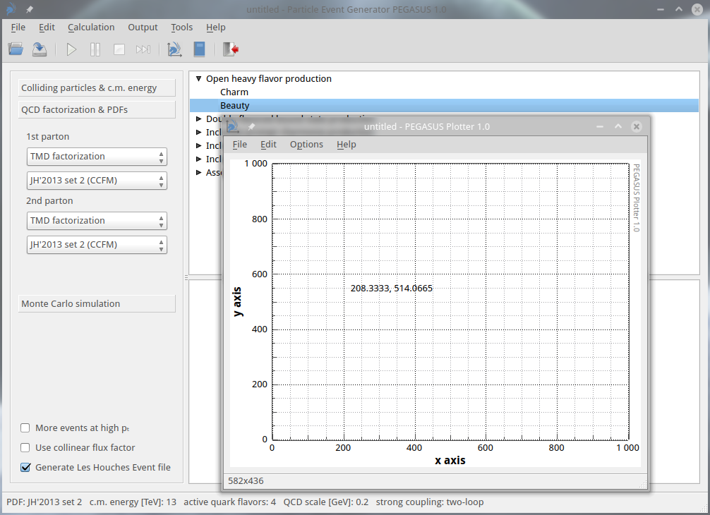
Figure 5: pegasus plotter can be launched from pegasus main window.

In general, off-shell initial states may cause violation of gauge invariance in the non-abelian theories. We solve this problem in a way[18]. We start with a set of ”extended” diagrams, where the off-shell gluons are considered as emitted by on-shell external fields (say, quarks), so that they represent internal lines in the Feynman graphs. As all of the external lines in these graphs are on shell, the gauge invariance of the whole set is fulfilled. However, the extended gauge invariant set may contain unfactorizable diagrams that cannot be represented as a convolution of the hard scattering amplitude and gluon density functions (such as, for example, Figs. 5(e) and 5(d) in[18]). At the same time, we learn from[18] that the non-factorizable diagrams vanish in the particular gauge (3). Therefore, within this gauge, we are left with the usual diagrams of the Parton Model.

In fact, the prescription (3) is a remake of Equivalent Photon Approximation (EPA) in QED and DIS. Consider a photon emitted by an electron: $e(p)\to e^{\prime}(p^{\prime})+\gamma(k)$. Then, taking trace over the electron line in the matrix element squared one obtains the polarization tensor

$$L^{\mu\nu}={\rm tr}\left[(\hat{p}^{\prime}+m_{e})\,\gamma^{\mu}\,(\hat{p}+m_{e})\,\gamma^{\nu}\right]=8\,p^{\mu}p^{\nu}-4(pk)\,g^{\mu\nu}.$$ (4)

Neglecting the second term in the right hand side in the small $x$ limit, $p\gg k$, one immediately arrives at the spin structure $\sum\epsilon^{\mu}\epsilon^{*\nu}\sim L^{\mu\nu}\sim p^{\mu}p^{\nu}$. It can be rewritten in the form (3) after using the Sudakov representation $k=xp+k_{T}$ and applying a gauge shift $\epsilon^{\mu}\to\epsilon^{\mu}-k^{\mu}/x$. The gauge invariance of the matrix element is correct to the accuracy of ${\cal O}(x)\simeq 10^{-4}-10^{-6}$.

2.3 CCFM evolution equation

The CCFM evolution equation[4] for TMD gluon density resums both BFKL[3] large logarithms $\alpha_{s}^{n}\ln^{n}1/x$ and $\alpha_{s}^{n}\ln^{n}1/(1-x)$ terms. In the limit of asymptotic energies, it is almost equivalent to BFKL, but also similar to usual DGLAP evolution[5] for large $x$. Moreover, it introduces angular ordering condition to treat correctly gluon coherence effects. In the leading logarthmic approximation (LLA), the CCFM equation for TMD gluon density $f_{g}(x,{\mathbf{k}}_{T}^{2},\mu^{2})$ can be written as

$$f_{g}(x,{\mathbf{k}}_{T}^{2},\mu^{2})=f_{g}^{(0)}(x,{\mathbf{k}}_{T}^{2},\mu_{0}^{2})\Delta_{s}(\mu,\mu_{0})+\atop{\displaystyle+\int\frac{dz}{z}\int\frac{dq^{2}}{q^{2}}\Theta(\mu-zq)\Delta_{s}(\mu,zq)\tilde{P}_{gg}(z,{\mathbf{k}}_{T}^{2},q^{2})f_{g}\left(\frac{x}{z},{\mathbf{k}}^{\prime\,2}_{T},q^{2}\right)},$$ (5)

where ${\mathbf{k}}_{T}^{\prime}={\mathbf{q}}(1-z)+{\mathbf{k}}_{T}$ and $\tilde{P}_{gg}(z,{\mathbf{k}}^{2}_{T},q^{2})$ is the CCFM splitting function:

$$\tilde{P}_{gg}(z,{\mathbf{k}}^{2}_{T},q^{2})=\bar{\alpha}_{s}(q^{2}(1-z)^{2})\left[\frac{1}{1-z}+\frac{z(1-z)}{2}\right]+\atop{\displaystyle+\bar{\alpha}_{s}({\mathbf{k}}_{T}^{2})\left[\frac{1}{z}-1+\frac{z(1-z)}{2}\right]\Delta_{ns}(z,{\mathbf{k}}^{2}_{T},q^{2})}.$$ (6)

The Sudakov and non-Sudakov form factors read:

$$\ln\Delta_{s}(\mu,\mu_{0})=-\int\limits_{\mu_{0}^{2}}^{\mu^{2}}\frac{d\mu^{\prime\,2}}{\mu^{\prime\,2}}\int\limits_{0}^{1-\mu_{0}/\mu^{\prime}}d\zeta\,\frac{\bar{\alpha}_{s}(\mu^{\prime\,2}(1-\zeta)^{2})}{1-\zeta},$$ (7)

$$\ln\Delta_{ns}(z,{\mathbf{k}}_{T}^{2},{\mathbf{q}}_{T}^{2})=-\bar{\alpha}_{s}({\mathbf{k}}_{T}^{2})\int\limits_{0}^{1}\frac{dz^{\prime}}{z^{\prime}}\int\frac{dq^{2}}{q^{2}}\Theta({\mathbf{k}}_{T}^{2}-q^{2})\Theta(q^{2}-z^{\prime\,2}{\mathbf{q}}^{2}_{T}).$$ (8)

where $\bar{\alpha}_{s}=3\alpha_{s}/\pi$. The first term in the CCFM equation is the initial TMD gluon density $f_{g}^{(0)}(x,{\mathbf{k}}_{T}^{2},\mu_{0}^{2})$ multiplied by the Sudakov form factor, decribing the contribution of non-resolvable branchings between the starting scale $\mu_{0}^{2}$ and scale $\mu^{2}$. The second term represents the details of the QCD evolution expressed by the convolution of the CCFM gluon splitting function $\tilde{P}_{gg}(z,{\mathbf{k}}^{2}_{T},q^{2})$ with the gluon density and Sudakov form factor. The angular ordering condition is introduced with the theta function, so the evolution scale $\mu^{2}$ is defined by the maximum allowed angle for any gluon emission[4]. The main advantage of this approach is the implicit including of higher-order radiative corrections (namely, a part of NLO + NNLO +… terms corresponding to the initial state real gluon emissions). Some details can be found, for example, in reviews[2].

A similar equation can be also written[19] for TMD valence quark densities with replacement of the gluon splitting function by the quark one. One usually takes the initial TMD gluon and valence quark distributions as

$$f_{g}^{(0)}(x,{\mathbf{k}}_{T}^{2},\mu_{0}^{2})=Nx^{-B}(1-x)^{C}\exp(-{\mathbf{k}}_{T}^{2}/\sigma^{2}),$$ (9)

$$f_{q_{v}}^{(0)}(x,{\mathbf{k}}_{T}^{2},\mu_{0}^{2})=xq_{v}(x,\mu_{0}^{2})\exp(-{\mathbf{k}}_{T}^{2}/\sigma^{2})/\sigma^{2},$$ (10)

where $\sigma=\mu_{0}/\sqrt{2}$ and $q_{v}(x,\mu^{2})$ is the conventional (collinear) quark density function. The parameters $N$, $B$ and $C$ can be fitted from collider data (see[19]).

The TMD (valence) quark densities for CCFM approach are not available in the current version of the pegasus.

2.4 Parton Branching approach

The Parton Branching (PB) method[21, 22] allows one to solve the DGLAP equations iteratively. It gives a possibility to take into account simultaneously soft-gluon emission at $z\to 1$ and transverse momentum $\mathbf{q}_{T}$ recoils in the parton branchings along the QCD cascade. The latter leads to a natural determination of TMD density functions for both gluons and quarks. A soft-gluon resolution scale $z_{M}$ is introduced to separate resolvable and non-resolvable emissions, which are treated via the DGLAP splitting functions $P_{ab}(\alpha_{s},z)$ and Sudakov form-factors, respectively. The PB equations for TMD parton densities read:

$$f_{a}(x,{\mathbf{k}}_{T}^{2},\mu^{2})=f_{a}^{(0)}(x,{\mathbf{k}}_{T}^{2},\mu_{0}^{2})\Delta_{a}(z_{M},\mu^{2},\mu^{2}_{0})+\sum_{b}\int\limits_{x}^{z_{M}}dz\int\frac{d^{2}\mathbf{q}}{\pi\mathbf{q}^{2}}\Theta(\mu^{2}-\mathbf{q}^{2})\times\atop{\displaystyle\times\Theta(\mathbf{q}^{2}-\mu_{0}^{2})\frac{\Delta_{a}(z_{M},\mu^{2},\mu^{2}_{0})}{\Delta_{a}(z_{M},\mathbf{q}^{2},\mu^{2}_{0})}P_{ab}^{(R)}(\alpha_{s}(\mathbf{q}^{2}),z)f_{b}\left(\frac{x}{z},{\mathbf{k}}_{T}^{\prime\,2},q^{2}\right)},$$ (11)

where $a=q$ or $g$ and ${\mathbf{k}}_{T}^{\prime}={\mathbf{q}}(1-z)+{\mathbf{k}}_{T}$. The Sudakov form factors are defined as

$$\ln\Delta_{a}(z_{M},\mu^{2},\mu^{2}_{0})=-\sum_{b}\int\limits_{\mu_{0}^{2}}^{\mu^{2}}\frac{d\mu^{\prime\,2}}{\mu^{\prime\,2}}\int\limits_{0}^{z_{M}}d\zeta\,\zeta\,P_{ba}^{(R)}(\alpha_{s}(\mu^{\prime\,2}),\zeta).$$ (12)

The real-emission branching probabilities $P_{ab}^{(R)}$ are obtained from splitting functions $P_{ab}$ by eliminating $\delta(1-z)$-terms and substituting $1/(1-z)_{+}\to 1/(1-z)$. The evolution scale $\mu^{2}$ can be connected with the emission angle with respect to the beam direction, that leads to the angular ordering condition $\mu=|{\mathbf{q}}_{T}|/(1-z)$. The dependence on the $z_{M}$ dissapears when this angular ordering condition is applied and $z_{M}$ is large enough. The initial TMD parton distributions are taken in a factorized form as a product of conventional quark and gluon densities and intrinsic transverse momentum distributions (taken in gaussian form [8, 9]), where all the parameters can be fitted from the collider data. Unlike the CCFM, the PB densities have the strong normalization property:

$$\int\limits_{0}^{\mu^{2}}f_{a}(x,{\mathbf{k}}_{T}^{2},\mu^{2})d{\mathbf{k}}_{T}^{2}=xa(x,\mu^{2}),$$ (13)

where $a=q$ or $g$ and $xa(x,\mu^{2})$ are the conventional parton density functions (PDFs). The PB equations can be solved numerically by an iterative Monte-Carlo method with the leading order (LO) or next-to-leading order (NLO) accuracy. The solution results in a steep decline of the parton densities at ${\mathbf{k}}_{T}^{2}>\mu^{2}$. It contrasts the CCFM evolution, where the transverse momentum is allowed to be larger than the scale $\mu^{2}$, corresponding to an effective taking into account higher-order contributions.

2.5 Kimber-Martin-Ryskin approach

The Kimber-Martin-Ryskin (KMR) approach[24] provides a technique to construct TMD gluon and quark densities from conventional ones by loosing the DGLAP strong ordering condition at the last evolution step, that results in $k_{T}$ dependence of the parton distributions. This procedure is believed to take into account effectively the major part of next-to-leading logarithmic (NLL) terms $\alpha_{s}(\alpha_{s}\ln\mu^{2})^{n-1}$ compared to the LLA, where terms proportional to $\alpha_{s}^{n}\ln^{n}\mu^{2}$ are taken into account.

At the LO, the KMR method, defined for ${\mathbf{k}}_{T}^{2}\geq\mu_{0}^{2}\sim 1$ GeV², results in expressions for TMD quark and gluon distributions[24]:

$$\displaystyle f_{q}(x,{\mathbf{k}}_{T}^{2},\mu^{2})=T_{q}({\mathbf{k}}_{T}^{2},\mu^{2})\frac{\alpha_{s}({\mathbf{k}}_{T}^{2})}{2\pi}\times\atop{\displaystyle\int\limits_{x}^{1}dz\left[P_{qq}^{\rm LO}(z)\frac{x}{z}q\left(\frac{x}{z},{\mathbf{k}}_{T}^{2}\right)\Theta\left(\Delta-z\right)+P_{qg}^{\rm LO}(z)\frac{x}{z}g\left(\frac{x}{z},{\mathbf{k}}_{T}^{2}\right)\right]},$$ (14)

$$\displaystyle f_{g}(x,{\mathbf{k}}_{T}^{2},\mu^{2})=T_{g}({\mathbf{k}}_{T}^{2},\mu^{2})\frac{\alpha_{s}({\mathbf{k}}_{T}^{2})}{2\pi}\times\atop{\displaystyle\int\limits_{x}^{1}dz\left[\sum_{q}P_{gq}^{\rm LO}(z)\frac{x}{z}q\left(\frac{x}{z},{\mathbf{k}}_{T}^{2}\right)+P_{gg}^{\rm LO}(z)\frac{x}{z}g\left(\frac{x}{z},{\bf k}_{T}^{2}\right)\Theta\left(\Delta-z\right)\right]},$$ (15)

where $P_{ab}^{\rm LO}(z)$ are the usual DGLAP splitting functions at LO and $\mu_{0}^{2}$ is the minimum scale for which DGLAP evolution is valid. The theta functions introduce the specific ordering conditions in the last evolution step, thus regulating the soft gluon singularities. The cut-off parameter $\Delta$ usually has one of two forms, $\Delta=\mu/(\mu+|{\mathbf{k}}_{T}|)$ or $\Delta=|{\mathbf{k}}_{T}|/\mu$, that reflects the angular or strong ordering conditions, respectively. In the case of angular ordering, the parton densities are extended into the ${\mathbf{k}}_{T}^{2}>\mu^{2}$ region, whereas the strong ordering condition leads to a steep drop of the parton distributions beyond the scale $\mu^{2}$. At low ${\mathbf{k}}_{T}^{2}<\mu_{0}^{2}$ the behaviour of the TMD parton densities has to be modelled[24]. Usually it is assumed to be flat under strong normalization condition (9).

The Sudakov form factors allow one to include logarithmic virtual (loop) corrections, they take the form:

$$T_{q}({\mathbf{k}}_{T}^{2},\mu^{2})=\exp\left[-\int\limits_{{\mathbf{k}}_{T}^{2}}^{\mu^{2}}\frac{d{\mathbf{q}}_{T}^{2}}{{\mathbf{q}}_{T}^{2}}\frac{\alpha_{s}({\mathbf{q}}_{T}^{2})}{2\pi}\int\limits_{0}^{z_{\text{max}}}d\zeta\,P_{qq}^{\text{LO}}(\zeta)\right],$$ (16)

$$T_{g}({\mathbf{k}}_{T}^{2},\mu^{2})=\exp\left[-\int\limits_{{\mathbf{k}}_{T}^{2}}^{\mu^{2}}\frac{d{\mathbf{q}}_{T}^{2}}{{\mathbf{q}}_{T}^{2}}\frac{\alpha_{s}({\mathbf{q}}_{T}^{2})}{2\pi}\left(\int\limits_{z_{\text{min}}}^{z_{\text{max}}}d\zeta\,\zeta P_{gg}^{\text{LO}}(\zeta)+n_{f}\int\limits_{0}^{1}d\zeta\,P_{gq}^{\text{LO}}(\zeta)\right)\right],$$ (17)

with $z_{\text{max}}=1-z_{\text{min}}=\mu/(\mu+|{\mathbf{q}}_{T}|)$. These form factors give the probability of evolving from a scale ${\mathbf{k}}_{T}^{2}$ to a scale $\mu^{2}$ without parton emission. At the NLO, the TMD parton densities can be written as[25]:

$$f_{a}(x,{\mathbf{k}}_{T}^{2},\mu^{2})=\int\limits_{0}^{1}dz\,T_{a}({\mathbf{p}}_{T}^{2},\mu^{2})\frac{\alpha_{s}({\mathbf{p}}_{T}^{2})}{2\pi}\sum_{b=q,g}P_{ab}^{\text{NLO}}(z)\frac{x}{z}b\left(\frac{x}{z},{\mathbf{p}}_{T}^{2}\right)\Theta(\Delta-z),$$ (18)

where ${\mathbf{p}}_{T}^{2}={\mathbf{k}}_{T}^{2}/(1-z)$. Note that both DGLAP splitting functions and conventional parton distributions should be taken with NLO accuracy. The Sudakov form factors at NLO read:

$$T_{q}({\mathbf{k}}_{T}^{2},\mu^{2})=\exp\left[-\int\limits_{{\mathbf{k}}_{T}^{2}}^{\mu^{2}}\frac{d{\mathbf{q}}_{T}^{2}}{{\mathbf{q}}_{T}^{2}}\frac{\alpha_{s}({\mathbf{q}}_{T}^{2})}{2\pi}\int\limits_{0}^{1}d\zeta\,\zeta(P_{qq}^{\text{NLO}}(\zeta)+P_{gq}^{\text{NLO}}(\zeta))\right],$$ (19)

$$T_{g}({\mathbf{k}}_{T}^{2},\mu^{2})=\exp\left[-\int\limits_{{\mathbf{k}}_{T}^{2}}^{\mu^{2}}\frac{d{\mathbf{q}}_{T}^{2}}{{\mathbf{q}}_{T}^{2}}\frac{\alpha_{s}({\mathbf{q}}_{T}^{2})}{2\pi}\int\limits_{0}^{1}d\zeta\,\zeta(P_{gg}^{\text{NLO}}(\zeta)+2n_{f}P_{qg}^{\text{NLO}}(\zeta))\right].$$ (20)

However, it was demonstrated that the NLO prescription, with a good accuracy, can be significantly simplified to keep only the LO splitting functions[25] while the main effect is related to the Sudakov form factors.

2.6 Flux factor

The choice of the flux factor is another peculiarity of off-shell calculations. The definition of the flux, which is the velocity of an off-shell particle, is highly disputable and is not clear. By default, we accepted the analytic continuation of the general textbook definition[17]:

$$F=2\lambda^{1/2}(\hat{s},k_{1}^{2},k_{2}^{2}).$$ (21)

Our choice is supported by a numerical experiment[26], where we have considered the production of $\chi_{cJ}$ states in a two photon process, $e+e\to\chi_{cJ}+e^{\prime}{+}e^{\prime}$ and made a comparison between the prompt calculation of this $2\to 3$ process and calculation based on EPA, $\gamma+\gamma\to\chi_{cJ}$ with $J=0$, $1$ or $2$. We find that the flux taken in the form (21) provides a sensibly better fit to the exact calcualtion. The fact that the exact calculation disagrees with the factorized (collinear) calculation indicates that the conditions for the factorization theorem are yet not fulfilled. In such a situation, our choice of the flux can be regarded as a phenomenological correction for non-factorizable contributions. The same definition of the flux is adopted, for example, in[10]. However, the user can optionally choose the conventional definition $F=2x_{1}x_{2}s$, as it is explained below.

3 Calculations using PEGASUS

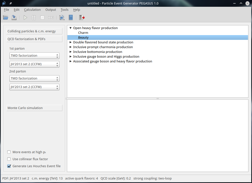
Figure 1: pegasus main window. Here one can select factorization scheme (TMD or collinear one) for each of the colliding particles, choose corresponding parton density function and set the parameters, important for further Monte-Carlo simulation: number of iterations and number of simulated events per iteration.

pegasus has an intuitive and unprecedentedly user friendly interface. The calcualtions using pegasus include a few general steps common for all of the processes. So, when pegasus is running, one can select the colliding particles, $pp$ or $p\bar{p}$, and set their center-of-mass energy $\sqrt{s}$. The default setting corresponds to the LHC Run II setup. Then one can select factorization scheme (TMD or collinear one) for each of the colliding particles, choose corresponding parton density function and set the parameters, important for further Monte-Carlo simulation, namely, number of iterations and number of simulated events per iteration (see Fig. 1). Next steps could be as follows (note that all these steps do not depend on each other and can be done in different order):

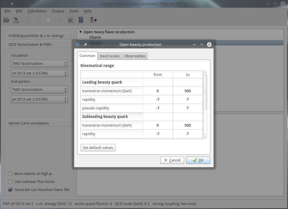
Figure 2: One can optionally correct the default kinematical restrictions, list of requested observables and corresponding binnings for any processes (part 1).

• From the list of available processes one can select the necessary process and then (optionally) correct the default kinematical restrictions, hard scales, list of requested observables and corresponding binnings (see Figs. 2 — 4). This can be done by double clicking on the requested process or via main menu (using Edit $\to$ Task option).

• For each of the observables one can manually edit the default binning according to own wishes. As another option, the binning can be uploaded immediately from the data file. Several commonly used formats (such as .yoda, .yaml, .csv or plain data format, compatible with gnuplot[27] tool) as provided by HepData repository[28] are supported.

• The user-defined setup for any process (total center-of-mass energy, selected parton densities, kinematical restrictions, binnings etc) can be saved to a configuration file in some internal format (*.pegasus). This can be done via the main menu (using File $\to$ Save or File $\to$ Save As options) or via the popup menu available on right mouse button click or via appropriate button in the button panel. Of course, the configuration file can be loaded and a user-defined setup can be used in further applications. This can be done via main menu (with File $\to$ Open option) or via popup menu or via Open button on the button panel.

• Weighted or unweighted events can be generated. This option is available via main menu Edit $\to$ Settings $\to$ Generated events or via popup menu.

• If one needs to generate the Les Houches Event file[29], one has to mark corresponding option before the calculation starts (see Fig. 1). Note that this option affects the speed of the calculations.

• The calculation will start by choosing the corresponding option in main menu (Calculation $\to$ Start), popup menu or pressing Start button on the button panel. The numerical results for requested observables will be immediately presented ”on the fly” with built-in tool pegasus plotter (see Fig. 5). The calculations can be paused or even stopped (using main menu options Calculation $\to$ Pause, Calculation $\to$ Stop, corresponding buttons on the button panel or options in popup menu). Of course, during pause in the calculations, all manipulations with accumulated results in pegasus plotter are allowed (see Section 4.3).

• If there are several contributing subprocesses, there is a possibility to immediately jump to the next one (via Calculation $\to$ Next option in main menu or appropriate button on button panel or popup menu) during the calculations.

The generated events can be accumulated in Les Houches Event (*.lhe) file and/or presented in pegasus plotter. Using the latter, one can save the results in a some internal format (*.pplot) or as a simple plain data (compatible, for example, with gnuplot package) or export them to an image (*.pdf, *.png, *.jpg or *.bmp).

Below we give a more detailed information and explanations about the important features of pegasus.

3.1 Parton density functions in a proton

Latest sets[19] of CCFM-evolved TMD gluon distributions in a proton, JH’2013 set 1 and JH’2013 set 2, are available in the pegasus. The input parameters of JH’2013 set 1 were determined from the fit to high precision HERA data on the proton structure function $F_{2}(x,Q^{2})$, whereas the parameters of JH’2013 set 2 gluon were extracted from combined fit on both $F_{2}(x,Q^{2})$ and $F_{2}^{c}(x,Q^{2})$ data (see [19]). The previous CCFM fits, namely, A0 and B0 sets[30], are available also and comparison between them can be found[19]. Technically, all these CCFM-evolved gluon densities are stored on a grid in $\log x$, $\log k_{T}$ and $\log\mu$ and a simple linear interpolation is applied to evaluated the gluon density for values in between the grid points. This interpolation proceeds automatically at the each event generation. The data files containing the grid points are supplied with the program package and read in at the beginning of each requested calculation.

The TMD gluon and quark densities can be also evaluated in the standard DGLAP scenario using the PB and/or KMR schemes (with LO or NLO accuracy). As an input for the KMR procedure, the conventional (collinear) PDFs have to be applied. Several sets of KMR and PB-based gluon densities are currently available in pegasus. So, well known NNPDF3.1 (LO)[32] and MMHT’2014 (LO)[13] parametrizations and recent analytical expressions obtained[33, 34, 35] in the so-called generalized double asymptotic scaling (DAS) approximation of QCD[34, 35] were used as an input. The DAS approximation is connected to the asymptotic behaviour of the DGLAP evolution discovered many years ago[36]. Flat initial conditions for the DGLAP equations, applied in the generalized DAS scheme, lead to the Bessel-like behaviour for the proton PDFs at small $x$[34, 35]. The DAS LO set 1 corresponds to ”frozen” treatment of the QCD strong coupling in the infrared region: $\alpha_{s}(\mu^{2})\to\alpha_{s}(\mu^{2}+m_{\rho}^{2})$. The DAS LO set 2 is based on the idea[37] regarding the analyticity of the strong coupling at low scales. The difference between these two choices is discussed[38]. Everywhere, the cut-off parameter $\Delta$ is taken according to angular ordering condition.

Set	Order of $\alpha_{s}$	$N_{f}$	$\Lambda_{\rm QCD}$/MeV	Ref.
A0 (CCFM)	1	4	250	[30]
B0 (CCFM)	1	4	250	[30]
JH’2013 set 1 (CCFM)	2	4	200	[19]
JH’2013 set 2 (CCFM)	2	4	200	[19]
KMR (MMHT’2014 LO)	1	5	211	[24]
KMR (NNPDF3.1 LO)	1	5	167	[24]
KMR (DAS LO set 1)	1	4	143	[38]
KMR (DAS LO set 2)	1	4	143	[38]
PB-NLO-HERAI+II’2018 set 1	2	4	118	[22]
PB-NLO-HERAI+II’2018 set 2	2	4	118	[22]

Table 1: The TMD gluon densities in a proton implemented into the pegasus. The A0$\pm$, B0$\pm$, JH’2013 set 1$\pm$ and JH’2013 set 2$\pm$ distributions, needed to estimate the scale uncertainties of the calculations (see below), are not shown.

The available TMD gluon sets with the essential parameters are listed in Table 1. We note that large variety of the TMD gluon distribution functions in a proton are collected in the tmdlib package[39], which is a C++ library providing a framework and an interface to the different parametrizations.

To perform the calculations in the collinear QCD factorization (mainly at LO or tree-level NLO for some processes) several sets of conventional PDFs are available in pegasus. These are recent MMHT’2014 (LO and NLO)[13] and CT14 (LO and NLO)[40] ones and previous sets provided by CTEQ Collaboration (CTEQ’6.6)[41], MSTW’2008 (LO and NLO)[42] and GRV’94 (LO)[43]. The standalone C++ codes from MMHT[13] and CTEQ[14] groups are implemented into the pegasus code and corresponding data files containing the grid points are supplied with the program package.

3.2 Simulated processes

Process	Subprocesses	Scales	Observables	Ref.
Open heavy flavor production	$g^{*}+g^{*}\to Q+\bar{Q}$	$p_{T}(Q)$	$p_{T}(Q)$	[44]
• charm		$m_{T}(Q)$	$y(Q)$
• beauty			$M(Q\bar{Q})$
			$\Delta\phi(Q\bar{Q})$
Double flavored bound state	$g^{*}+g^{*}\to{\cal Q}+b+\bar{c}$	$p_{T}({\cal Q})$	$p_{T}({\cal Q})$	[45]
production		$m_{T}({\cal Q})$	$y({\cal Q})$
• $B_{c}$
• $B_{c}^{(*)}$
$S$-wave heavy quarkonia	$g^{*}+g^{*}\to Q\bar{Q}[^{3}S^{(1)}_{1}]+g\to{\cal Q}+g$	$p_{T}({\cal Q})$	$p_{T}({\cal Q})$	[46, 47]
production	$g^{*}+g^{*}\to Q\bar{Q}[^{1}S^{(8)}_{0}]\to{\cal Q}$	$m_{T}({\cal Q})$	$y({\cal Q})$
• $J/\psi$	$g^{*}+g^{*}\to Q\bar{Q}[^{3}S^{(8)}_{1}]\to{\cal Q}$
• $\psi^{\prime}$	$g^{*}+g^{*}\to Q\bar{Q}[^{3}P^{(8)}_{J}]\to{\cal Q}$
• $\Upsilon(3S)$
$P$-wave heavy quarkonia	$g^{*}+g^{*}\to Q\bar{Q}[^{3}P^{(1)}_{J}]\to{\cal Q}$	$p_{T}({\cal Q})$	$p_{T}({\cal Q})$	[46, 47]
production	$g^{*}+g^{*}\to Q\bar{Q}[^{3}S^{(8)}_{1}]\to{\cal Q}$	$m_{T}({\cal Q})$	$y({\cal Q})$
• $\chi_{cJ}(1P)$
• $\chi_{bJ}(3P)$
Inclusive Higgs production	$g^{*}+g^{*}\to H^{0}$	$m(H^{0})$	$p_{T}(H^{0})$	[48]
• $H^{0}\to\gamma\gamma$		$m_{T}(H^{0})$	$y(H^{0})$
• $H^{0}\to ZZ^{*}\to 4l$			$|\cos\theta^{*}|$
• $H^{0}\to W^{+}W^{-}\to e^{\pm}\mu^{\mp}\nu\bar{\nu}$			$\Delta\phi(\gamma\gamma)$
			$m_{34}(ll)$
			$y(ll)$
Associated gauge boson and	$g^{*}+g^{*}\to V+Q+\bar{Q}$	$p_{T}(\gamma)$	$p_{T}(V)$	[49, 50]
heavy flavor production	$g+Q\to V+Q$	$p_{T}(Q)$	$p_{T}(Q)$
• $\gamma+Q$	$q+Q\to V+q+Q$	$m(Z/\gamma^{*})$	$y(V)$
• $Z/\gamma^{*}+Q$	$q+\bar{q}\to V+Q+\bar{Q}$	$m_{T}(Z/\gamma^{*})$	$y(Q)$
			$\Delta R(ZQ)$
			$\Delta\phi(ZQ)$

Table 2: List of the available processes. Note that exact definitions of all kinematical variables can be found, for example, in corresponding references.

List of processes, currently available in the pegasus, is presented in Table 2. We would like to clarify some points, which are not mentioned in the Table 2:

• $Q$ denotes a heavy ($c$ or $b$) quark, ${\cal Q}$ denotes $B_{c}$, $B_{c}^{(*)}$, $J/\psi$, $\psi^{\prime}$, $\Upsilon(3S)$, $\chi_{cJ}(1P)$ or $\chi_{bJ}(3P)$ mesons with $J=0$, $1$ or $2$, $V$ stands for $\gamma$ or $Z/\gamma^{*}$ and $l=e$ or $\mu$.

• The standard spectroscopic notation ${}^{(2S+1)}L_{J}^{(a)}$ is used for intermediate Fock state of heavy quark pair $Q\bar{Q}$ produced with spin $S$, orbital angular momentum $L$, total angular momentum $J$ and color representation $a$.

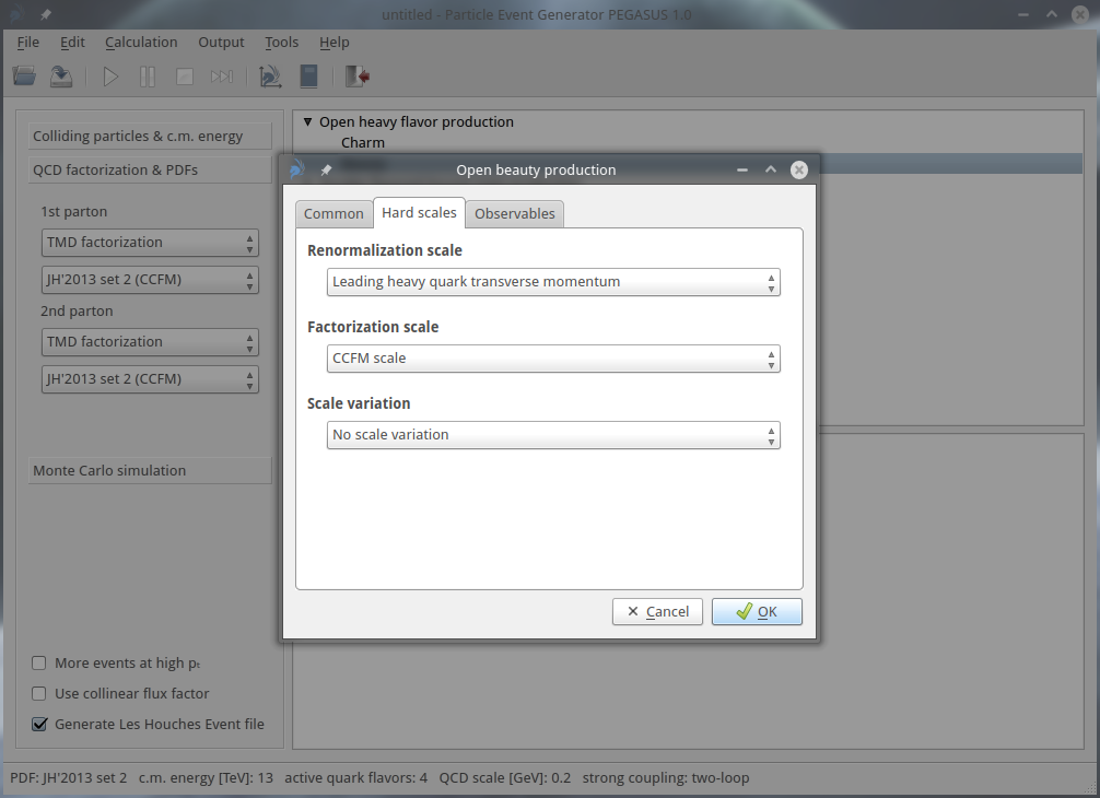
Figure 3: One can optionally correct the default kinematical restrictions, list of requested observables and corresponding binnings for any processes (part 2).

• Besides the scales, listed in the Table 2, for every process some universal scales are available, namely: total energy of the partonic subprocess $\sqrt{\hat{s}}$, also $\sqrt{\hat{s}/4}$ and so-called CCFM scale $\sqrt{\hat{s}+\mathbf{Q}_{T}^{2}}$[19, 30], where $\mathbf{Q}_{T}$ is the total tranverse momentum of the final partons, see Fig. 3.

• To estimate the scale uncertainties, the hard scales above can be varied around its default value by a factor of $2$ or $1/2$, as it often done in the pQCD calculations. This applies to any scale, except the CCFM scale. For CCFM-based gluon densities the scale uncertainties are evaluated by a change of the default gluon distribution to so-called ”+” and ”–” ones of the corresponding set[19, 30].

• Part of the non-logarithmic loop corrections to effective $g^{*}+g^{*}\to H^{0}$ vertex can be absorbed in the special $K$-factor[51] and optionally implemented into the calculations. As default choice, this $K$-factor is switched off.

• According to experimental setup, an isolation criterion is applied for prompt photon production. This criterion is the following: a photon is isolated if the amount of hadronic transverse energy $E_{T}^{\rm had}$ deposited inside a cone with aperture $R$ centered around the photon direction in the pseudo-rapidity and azimuthal angle plane, is smaller than some value $E_{T}^{\rm max}$ (”cone isolation”). The isolation requirement significantly (up to $\sim 10$% of the visible cross section) reduces contribution from the so-called photon fragmentation mechanisms, not implemented into the pegasus. The isolation criterion and additional conditions which preserve our calculations from divergences have been specially discussed, for example, in[52] (see also references therein). The default values $R=0.4$ and $E_{T}^{\rm max}=4$ GeV can be changed optionally.

• At present, quark-initiated subprocesses can be calculated only within collinear QCD factorization and no TMD quark densities are implemented into the current version of pegasus. The QCD Compton subprocess is available only, if collinear factorization has been chosen, since in the $k_{T}$-factorization approach its contribution is taken into account by the off-shell gluon-gluon fusion (see[49, 50] for more details).

3.3 Quarkonium final states

Quarkonium production processes need additional explanations as they contain an important extra step: the formation of bound states.

The process starts with the production of a heavy quark-antiquark pair $Q\bar{Q}$ in a hard parton interaction. The produced quark pair may be either color singlet or color octet. If the $Q\bar{Q}$ state is color singlet, it can immediately convert into a meson with appropriate quantum numbers. Then the formation probability is determined by a single parameter, the radial wave function at the origin of the coordinate space, $|{\cal R}_{S}(0)|^{2}$ or $|{\cal R}^{\prime}_{P}(0)|^{2}$[53, 54, 55, 56, 57]. The values of these functions can be extracted from the measured decay widths or calculated within potential models.

The situation with color-octet states is more complicated as the transition to a color-singlet physical hadron requires the emission of extra (soft) gluons. Then, for every final state hadron $h$ and for every intermediate $Q\bar{Q}$ state $n=\,^{2S+1}L_{J}$ listed in Table 2 there is a specific phenomenological long-distance matrix element (LDME)[58, 59, 60] responsible for such a transition $\langle{\cal O}^{h}\left[n\right]\rangle$. Eventually, the production cross section for a hadron $h$ in $pp$ collisions is given by a sum over all possible singlet and octet $Q\bar{Q}$ states:

$$\sigma(pp\to h+X)=\sum_{n}\sigma\left(pp\to Q\bar{Q}\left[n\right]\right)\langle{\cal O}^{h}\left[n\right]\rangle,$$ (22)

where $\sigma\left(pp\to Q\bar{Q}\left[n\right]\right)$ is the partial partonic cross section (1) for a $Q\bar{Q}$ state $n$. The different states $n$ are selected by introducing the proper projection operators in the hard scattering amplitude. The correspondence between the color singlet and color octet wave functions and respective LDMEs is given by the $\langle{\cal O}^{h}\left[\,{}^{2S+1}L_{J}\right]\rangle=2N_{c}(2J+1)|{\cal R}_{S}(0)|^{2}/{4\pi}$ and $\langle{\cal O}^{h}\left[\,{}^{2S+1}L_{J}\right]\rangle=6N_{c}(2J+1)|{\cal R}_{P}^{\prime}(0)|^{2}/{4\pi}$, respectively.

As default choice to describe the spin structure of relevant transition amplitudes, pegasus uses the model[61], where the NRQCD emission of soft gluons is considered in terms of classical multipole radiation theory. The multipole expansion is dominated by (chromo)electric dipole transitions $E1$. According to[61], only a single $E1$ transition is needed to transform a $P$-wave state into an $S$-wave state and the structure of the respective ${{}^{3}P_{J}^{(8)}}\to{{}^{3}S_{1}^{(1)}}+g$ amplitudes is taken the same as for radiative decays of $\chi_{cJ}$ mesons[62, 63]:

$${\cal A}(\,^{3}P_{0}^{(8)}\to\,^{3}S_{1}^{(1)}+g)\sim k_{\mu}\,p^{\mu}\,\epsilon_{\nu}(l)\epsilon^{\nu}(k),$$ (23)

$${\cal A}(\,^{3}P_{1}^{(8)}\to\,^{3}S_{1}^{(1)}+g)\sim e^{\mu\nu\alpha\beta}k_{\mu}\,\epsilon_{\nu}(p)\,\epsilon_{\alpha}(l)\epsilon_{\beta}(k),$$ (24)

$${\cal A}(\,^{3}P_{2}^{(8)}\to\,^{3}S_{1}^{(1)}+g)\sim p^{\mu}\,\epsilon^{\alpha\beta}(p)\,\epsilon_{\alpha}(l)\left[k_{\mu}\epsilon_{\beta}(k)-k_{\beta}\epsilon_{\mu}(k)\right],$$ (25)

where $p$, $k$ and $l=p-k$ are the four-momenta of the color-octet $P$-wave state, emitted gluon and produced color-singlet $S$-wave state, $\epsilon^{\mu}(k)$, $\epsilon^{\mu}(l)$, $\epsilon^{\mu}(p)$ and $\epsilon^{\mu\nu}(p)$ are the polarization vectors (tensor) of respective particles and $e^{\mu\nu\alpha\beta}$ is the fully antisymmetric Levi-Civita tensor. The transformation of an $S$-wave state into another $S$-wave state (such as $J/\psi$ or $\psi^{\prime}$ meson) is treated as two successive $E1$ transitions ${}^{3}S_{1}^{(8)}\to\,^{3}P_{J}^{(8)}+g$, ${}^{3}P_{J}^{(8)}\to\,^{3}S_{1}^{(1)}+g$ proceeding via either of the three intermediate states: ${}^{3}P_{0}^{(8)}$, ${}^{3}P_{1}^{(8)}$, or ${}^{3}P_{2}^{(8)}$. For each of the two transitions the same effective coupling vertices (23) — (25) are exploited. In the case of $J/\psi$ or $\Upsilon(3S)$ production, the user can optionally include feed-down from the decays of upper quarkonium states ($\psi^{\prime}$, $\chi_{cJ}(1P)$ or $\chi_{bJ}(3P)$, respectively) in addition to the direct production channels.

The absolute normalization of the transition amplitudes is not calculable within the theory; these numbers are taken as free adjustable parameters. However, the values of the LDMEs for the different partial contributions are not completely independent but are connected by the heavy quark spin symmetry (HQSS) relations[60]. All the HQSS relations between LDMEs are implemented in the pegasus default setting, taken from[46, 47].

3.4 Strong coupling and masses of particles

In pegasus, the strong coupling $\alpha_{s}$ can be calculated in one-loop or two-loop approximation with respect to the number of active flavors $N_{f}$ and $\Lambda_{\rm QCD}$. The choice of $N_{f}$ and $\Lambda_{\rm QCD}$ is done automatically (according to the Table 1) with the choice of the TMD and/or conventional parton density in a proton. There is no possibility to change it manually since this setup is essential for determination of corresponding parton distributions.

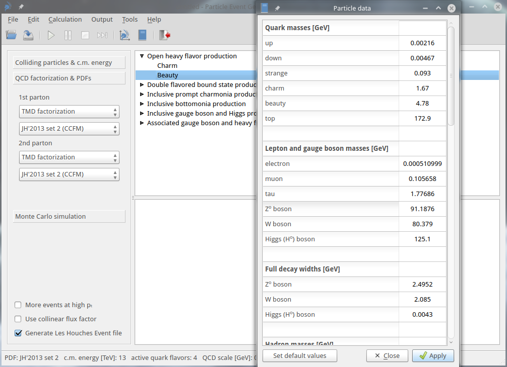
Figure 6: Particle data tool can be launched from pegasus main window.

The masses of all particles (quarks, gauge bosons, heavy quarkonia etc), their branching ratios and decay widths are fixed according to Particle Data Group (PDG)[64]. Any of these parameters can be easily changed using the convenient built-in particle data tool (see Fig. 6), which is available via main menu (Edit $\to$ Settings $\to$ Particle data) or popup menu or appropriate button on the button panel.

3.5 Generation of Les Houches Event file

pegasus is supplied with a tool to construct event files in the Les Houches Event format[29]. This is a widely accepted format to present events, which is compatible with the majority of modern general purpose Monte-Carlo generators.

The Les Houche Event (LHE) file, generated by the pegasus, consists of two main blocks: the first one contains the information about the number of the recorded events, the PDFs used, the colliding hadrons and their energies. Also the total cross section is shown. The second block represents a list of events, including the data on the interacting partons, their 4-momenta and color structure of the event. We mention the basic features of the LHE file, generated by the pegasus:

• The generated events could be weighted or unweighted. In first case, the sum of all the weights is the total cross section of the subprocess.

• Polarization information is not preserved.

• A parton carries a tag according to the standard PDG numbering scheme[64].

• Conventional (collinear) parton densities in a proton are numbered according to the lhapdf scheme[65] while TMD parton distributions are numbered according to the tmdlib package[39].

The produced LHE file can then be processed with an external program to introduce some peculiar event selection, to include parton showers, to hadronize the final particles, etc. It is found to be compatible with such Monte Carlo generators as pythia[6] and cascade[9].

4 Program components

4.1 Random number generator

Since all the internal variables in pegasus are declared as double precision ones, double precision random numbers have to be generated in the Monte-Carlo simulations. The random number generator ranlux[66] is well suited for these purposes. It has a long period, solid theoretical foundations and is commonly used in computational physics. This random number generator is implemented into the pegasus.

4.2 Phase space integration and event generation

The multidimensional phase space integration (1) is performed with the Monte-Carlo technique and is incorporated with the routine vegas[12]. The routine vegas allows up to ten integration variables, that is enough for subprocesses considered in pegasus.

The vegas algorithm is based on a method for reducing statistical errors by using a known probability distribution function to concentrate the search in those areas of the integrand that make the greatest contribution to the final integral.

The algorithm is realised through a large number of random sample points distributed over a $d$-dimensional rectangular volume. The whole volume is divided into $d$-dimensional rectangular cells (by default, 50 divisions along each axis). The probability for a point to drop into a given cell is determined by so called sampling distribution, which is adjusted to the integrand function. The sampling distribution approximates the exact distribution by making a number of passes (iterations) over the integration region while histogramming the integrand function $d\sigma$ given by the expession (1). Each iteration is used to define a sampling distribution for the next iteration. To improve the convergence in the region of high $p_{T}$, the user can optionally modify the integrand function from $d\sigma$ to $(1+p_{T}^{4})d\sigma$, see Fig. 1. The optimization of the sample grid is made automatically and needs no care from the user.

Each sample point generated by vegas represents an event in the $n$-particle phase space with the coordinates of the sample point responding to the values of the physical integration variables ($p_{iT}$, $y_{i}$, $\phi_{i}$). The weight attributed to that event is given by the product of the integrand function $d\sigma$ and the $d$-volume of the sampling cell containing that point, $dw=d\sigma dV_{\rm cell}$. Unweighting algorithm for the generated events is provided also.

The typical time needed to generate one event, of course, depends on the requested subprocess; but, in general, is similar to time needed by other Monte-Carlo event generators like cascade or pythia. The output events can be plotted on a histogram (using built-in tool pegasus plotter ) or stored for further use in the form of an Les Houches Event file.

4.3 PEGASUS Plotter

pegasus is supplied with a built-in tool pegasus plotter, allowing one to depict easily the produced differential cross sections and immediately compare them with experimental data. As a default setting, the accumulated results for requested observables during the calculation are shown in pegasus plotter. However, it is a quite independent tool and can be used apart from any calculations made within the pegasus. The program is very simple and intuitive. Let us briefly describe main features of the tool.

As one calls the pegasus plotter from the main menu of the pegasus (using the Tool $\to$ Plotter option, or via popup menu, or by pressing the corresponding button on button panel) an empty sheet is created. The following objects, stored in a plain data files, could be added to the sheet (by choosing Edit $\to$ Add option in the main menu or popup menu available with a right mouse button click on the sheet):

• Curve. The data file should consist of two columns, corresponding to the rows of $x$ and $y$ values.

• Histogram. The data file is the same, as for Curve. However, every $y$ value should be mentioned twice, for the both borders of the corresponding bin.

• Filled area. A three-columns data file should contain for every $x$ value lower and upper values of $y$.

• Text label. An arbitrary text note inside the plot sheet. Greek letters are available through the syntax {/Symbol letter}, where the letter is just the name of the greek symbol (for instance, alpha, sigma or other). Several capital greek symbols are available, namely, $\Upsilon$ ({/Symbol Upsilon}), $\Psi$ ({/Symbol Psi}) and $\Delta$ ({/Symbol Delta}). Subscripts and superscripts are available with a latex-like syntax _{subscript}, ^{superscript}.

• Experimental data. The data file should be in gnuplot-compatible format with 6 columns, corresponding to $x$, $y$, lower and upper $x$ values and lower and upper $y$ values. Alternatively, the data files in standard *.yoda or *.csv format (available from HepData repository[28]) can be uploaded.

As an object is added on the sheet, it can be selected with a left mouse button click and modified according to user own wishes either with a double click or with choosing option Edit$\to$ Plottable in the pegasus plotter main menu or via popup menu. Then the text label in the legend and appearance of the selected object (for example, color, font, size etc) can be changed. If selected object is a Histogram, the fiducial cross section (integral with respect to the $x$ variable) is shown in the status bar. One can also set a factor to scale the depicted cross sections using Edit $\to$ Multiply by a factor option in main menu or popup menu.

The default axes setting can be changed from the main menu (Edit $\to$ Axes option) or by double clicking an axis. Besides the font, alignment and other setting one can also set the axes to be linear or logarithmic. From the main menu (Options $\to$ Plot size) or popup menu one can also adjust the size of the graph in pixels.

The plot can be saved for the future editing via main menu options File $\to$ Save or File $\to$ Save As or via popup menu in the internal format (*.pplot). The export to a gnuplot script is possible via main menu Export $\to$ Plot to Gnuplot script option or via popup menu. The figure can be also printed out or saved in *.png, *.jpg or *.bmp format. Finally, samples for all plotted curves, histograms or data point sets (or for only selected ones) can be transfered (using Options $\to$ Export) to a plain data file (which is compatible, for example, with gnuplot) for future usage in other programs.

Some typical snapshots of the pegasus plotter are presented on Fig. 7.

5 Installation and running

pegasus can be downloaded from https://theory.sinp.msu.ru/dokuwiki/doku.php/pegasus/download as a precompiled executive file for Linux machines. No special installation procedure is needed. The data files containing the necessary TMD parton densities in a proton (and conventional PDFs as well) are located inside the pegasus home directory (folder data). If there are some missing data files in data folder, pegasus will inform user about that (see Fig. ?). In this case, no calculation is allowed. Location of data folder could be easily changed via main menu option Edit $\to$ Settings $\to$ Path to data folder.

For Linux machines, the executive file can be just run from a terminal as ./PEGASUS. The program demands the qwt library (version 6.1.3)[11], so the library file libqwt.so.6 should be inside the pegasus home directory. Otherwise, the path to this file should be specified with export LD_LIBRARY_PATH=/path/to/library.

The program was tested on ROSA Linux R8.1, ROSA Linux R11 and Ubuntu 16.04.

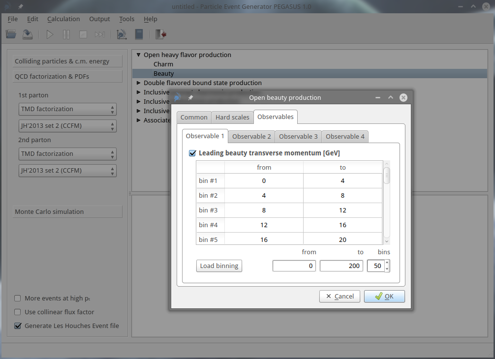
Figure 4: One can optionally correct the default kinematical restrictions, list of requested observables and corresponding binnings for any processes (part 3).

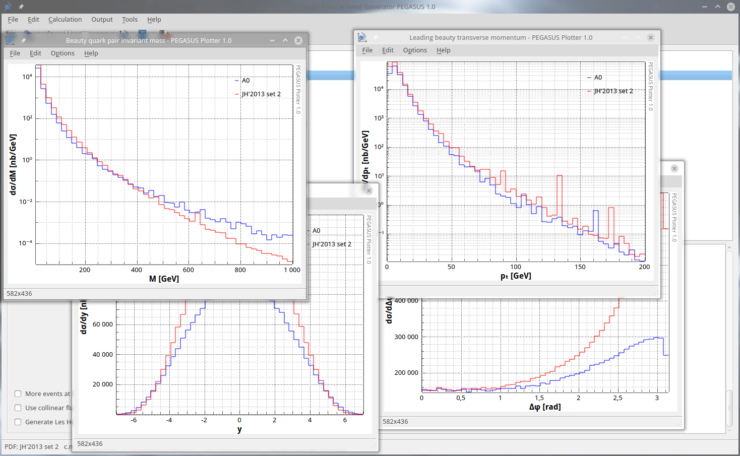
Figure 7: Results of the calculations presented by pegasus plotter.

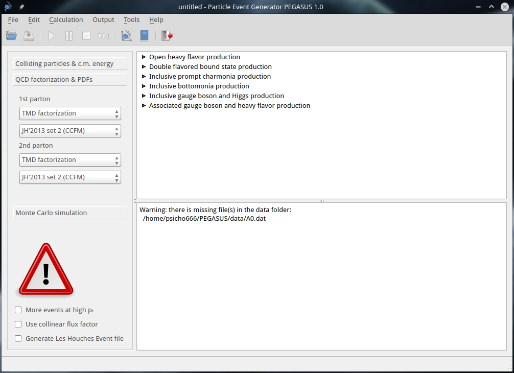
Figure 8: If there are some missing data files in data folder, pegasus informs user about that.

References

- [1] R. Angeles-Martinez, A. Bacchetta, I.I. Balitsky, D. Boer, M. Boglione, R. Boussarie, F.A. Ceccopieri, I.O. Cherednikov, P. Connor, M.G. Echevarria, G. Ferrera, J. Grados Luyando, F. Hautmann, H. Jung, T. Kasemets, K. Kutak, J.P. Lansberg, A. Lelek, G.I. Lykasov, J.D. Madrigal Martinez, P.J. Mulders, E.R. Nocera, E. Petreska, C. Pisano, R. Placakyte, V. Radescu, M. Radici, G. Schnell, I. Scimemi, A. Signori, L. Szymanowski, S. Taheri Monfared, F.F. van der Veken, H.J. van Haevermaet, P. van Mechelen, A.A. Vladimirov, S. Wallon, Acta Phys. Polon. B 46, 2501 (2015).
-
[2]
B. Andersson et al. (Small-x Collaboration), Eur. Phys. J. C 25, 77 (2002);
J. Andersen et al. (Small-x Collaboration), Eur. Phys. J. C 35, 67 (2004);
J. Andersen et al. (Small-x Collaboration), Eur. Phys. J. C 48, 53 (2006). -
[3]
E.A. Kuraev, L.N. Lipatov, V.S. Fadin, Sov. Phys. JETP 44, 443 (1976);
E.A. Kuraev, L.N. Lipatov, V.S. Fadin, Sov. Phys. JETP 45, 199 (1977);
I.I. Balitsky, L.N. Lipatov, Sov. J. Nucl. Phys. 28, 822 (1978). -
[4]
M. Ciafaloni, Nucl. Phys. B 296, 49 (1988);
S. Catani, F. Fiorani, G. Marchesini, Phys. Lett. B 234, 339 (1990);
S. Catani, F. Fiorani, G. Marchesini, Nucl. Phys. B 336, 18 (1990);
G. Marchesini, Nucl. Phys. B 445, 49 (1995). -
[5]
V.N. Gribov, L.N. Lipatov, Sov. J. Nucl. Phys. 15, 438 (1972);
L.N. Lipatov, Sov. J. Nucl. Phys. 20, 94 (1975);
G. Altarelli, G. Parisi, Nucl. Phys. B 126, 298 (1977);
Yu.L. Dokshitzer, Sov. Phys. JETP 46, 641 (1977). - [6] T. Sjöstrand, S. Ask, J.R. Christiansen, R. Corke, N. Desai, P. Ilten, S. Mrenna, S. Prestel, C.O. Rasmussen, P.Z. Skands, Comput. Phys. Commun. 191, 159 (2015).
- [7] J. Campbell, T. Neumann, arXiv:1909.09117 [hep-ph].
- [8] J. Alwall, R. Frederix, S. Frixione, V. Hirschi, F. Maltoni, O. Mattelaer, H.-S. Shao, T. Stelzer, P. Torrielli, M. Zaro, JHEP 07, 079 (2014).
-
[9]
https://cascade.hepforge.org;
H. Jung, S.P. Baranov, M. Deak, A. Grebenyuk, F. Hautmann, M. Hentschinski, A. Knutsson, M. Krämer, K. Kutak, A. Lipatov, N. Zotov, Eur. Phys. J. C 70, 1237 (2010). - [10] A. van Hameren, Comput. Phys. Commun. 224, 371 (2018).
- [11] https://qwt.sourceforge.io
- [12] G.P. Lepage, J. Comput. Phys. 27, 192 (1978).
- [13] L.A. Harland-Lang, A.D. Martin, P. Motylinski, R.S. Thorne, Eur. Phys. J. C 75, 204 (2015).
- [14] https://hep.pa.msu.edu/cteq/public
-
[15]
S. Catani, M. Ciafaloni, F. Hautmann, Nucl. Phys. B 366, 135 (1991);
J.C. Collins, R.K. Ellis, Nucl. Phys. B 360, 3 (1991). -
[16]
L.V. Gribov, E.M. Levin, M.G. Ryskin, Phys. Rep. 100, 1 (1983);
E.M. Levin, M.G. Ryskin, Yu.M. Shabelsky, A.G. Shuvaev, Sov. J. Nucl. Phys. 53, 657 (1991). - [17] E. Bycling, K. Kajantie, Particle Kinematics, John Wiley and Sons, New York (1973).
- [18] J.C. Collins, R.K. Ellis, Nucl. Phys. B 360, 3 (1991).
- [19] F. Hautmann, H. Jung, Nucl. Phys. B 883, 1 (2014).
- [20] F. Hautmann, M. Hentschinski, H. Jung, Nucl. Phys. B 865, 54 (2012).
- [21] F. Hautmann, H. Jung, A. Lelek, V. Radescu, R. Zlebcik, Phys. Lett. B 772, 446 (2017).
- [22] F. Hautmann, H. Jung, A. Lelek, V. Radescu, R. Zlebcik, JHEP 1801, 070 (2018).
- [23] S. Taheri Monfared, F. Hautmann, H. Jung, M. Schmitz, arXiv:1908.01621 [hep-ph].
-
[24]
M.A. Kimber, A.D. Martin, M.G. Ryskin, Phys. Rev. D 63, 114027 (2001);
A.D. Martin, M.G. Ryskin, G. Watt, Eur. Phys. J. C 31, 73 (2003). - [25] A.D. Martin, M.G. Ryskin, G. Watt, Eur. Phys. J. C 66, 163 (2010).
- [26] S.P. Baranov, A. Szczurek, Phys. Rev. D 77, 054016 (2008).
- [27] www.gnuplot.info
- [28] https://www.hepdata.net
- [29] J. Alwall, A. Ballestrero, P. Bartalini, S. Belov, E. Boos, A. Buckley, J.M. Butterworth, L. Dudko, S. Frixione, L. Garren, S. Gieseke, A. Gusev, I. Hinchliffe, J. Huston, B. Kersevan, F. Krauss, N. Lavesson, L. Lönnblad, E. Maina, F. Maltoni, M.L. Mangano, F. Moortgat, S. Mrenna, C.G. Papadopoulos, R. Pittau, P. Richardson, M.H. Seymour, A. Sherstnev, T. Sjöstrand, P. Skands, S.R. Slabospitsky, Z. Wcas, B.R. Webber, M. Worek, D. Zeppenfeld, Comput. Phys. Commun. 176, 300 (2007).
- [30] H. Jung, arXiv:hep-ph/0411287.
- [31] F. Hautmann, H. Jung, S. Taheri Monfared, Eur. Phys. J. C 74, 3082 (2014).
- [32] NNPDF Collaboration, Eur. Phys. J. C 77, 663 (2017).
- [33] G. Cvetic, A.Yu. Illarionov, B.A. Kniehl, A.V. Kotikov, Phys. Lett. B 679, 350 (2009).
- [34] A.V. Kotikov, G. Parente, Nucl. Phys. B 549, 242 (1999).
- [35] A.Yu. Illarionov, A.V. Kotikov, G. Parente, Phys. Part. Nucl. 39, 307 (2008).
- [36] A. de Rujula, S.L. Glashow, H.D. Politzer, S.B. Treiman, F. Wilczek, A. Zee, Phys. Rev. D 10, 1649 (1974).
-
[37]
D.V. Shirkov, I.L. Solovtsov, Phys. Rev. Lett. 79, 1209 (1997);
I.L. Solovtsov, D.V. Shirkov, Theor. Math. Phys. 120, 1220 (1999). - [38] A.V. Kotikov, A.V. Lipatov, B.G. Shaikhatdenov, P. Zhang, arXiv:1911.01445 [hep-ph].
- [39] F. Hautmann, H. Jung, M. Krämer, P.J. Mulders, E.R. Nocera, T.C. Rogers, A. Signori, Eur. Phys. J. C 74, 3220 (2014).
- [40] S. Dulat, T.J. Hou, J. Gao, M. Guzzi, J. Huston, P. Nadolsky, J. Pumplin, C. Schmidt, D. Stump, C.-P. Yuan, Phys. Rev. D 93, 033006 (2016).
- [41] P. Nadolsky, H.-L. Lai, Q.-H. Cao, J. Huston, J. Pumplin, D. Stump, W.-K. Tung, C.-P. Yuan, Phys. Rev. D 78, 013004 (2008).
- [42] A.D. Martin, W.J. Stirling, R.S. Thorne, G. Watt, Eur. Phys. J. C 63, 189 (2009).
- [43] M. Glück, E. Reya, A. Vogt, Z. Phys. C 67, 433 (1995).
- [44] H. Jung, M. Krämer, A.V. Lipatov, N.P. Zotov, JHEP 1101, 085 (2011).
- [45] S.P. Baranov, A.V. Lipatov, Phys. Lett. B 785, 338 (2018).
- [46] S.P. Baranov, A.V. Lipatov, arXiv:1906.07182 [hep-ph].
- [47] N.A. Abdulov, A.V. Lipatov, Eur. Phys. J. C 79, 830 (2019).
- [48] N.A. Abdulov, A.V. Lipatov, M.A. Malyshev, Phys. Rev. D 97, 054017 (2018).
- [49] A.V. Lipatov, M.A. Malyshev, N.P. Zotov, JHEP 05, 104 (2012).
- [50] S.P. Baranov, H. Jung, A.V. Lipatov, M.A. Malyshev, Eur. Phys. J. C 77, 772 (2017).
- [51] G. Watt, A.D. Martin, M.G. Ryskin, Phys. Rev. D 70, 014012 (2004).
- [52] A.V. Lipatov, M.A. Malyshev, Phys. Rev. D 94, 034020 (2016).
- [53] C.-H. Chang, Nucl. Phys. B 172, 425 (1980).
- [54] E.L. Berger, D. Jones, Phys. Rev. D 23, 1521 (1981).
- [55] R. Baier, R. Rückl, Phys. Lett. B 102, 364 (1981).
- [56] H. Krasemann, Z. Phys. C 1, 189 (1979).
- [57] G. Guberina, J. Kühn, R. Peccei, R. Rückl, Nucl. Phys. B 174, 317 (1980).
- [58] G. Bodwin, E. Braaten, P. Lepage, Phys. Rev. D 46, R1914 (1992).
- [59] E. Braaten, T.-C. Yuan, Phys. Rev. D 50, 3176 (1994).
-
[60]
G. Bodwin, E. Braaten, P. Lepage, Phys. Rev. D 51, 1125 (1995);
G. Bodwin, E. Braaten, P. Lepage, Phys. Rev. D 55, 5853(E) (1997). - [61] S.P. Baranov, Phys. Rev. D 93, 054037 (2016).
- [62] A.V. Batunin, S.R. Slabospitsky, Phys. Lett. B 188, 269 (1987).
- [63] P. Cho, M. Wise, S. Trivedi, Phys. Rev. D 51, R2039 (1995).
- [64] PDG Collaboration, Phys. Rev. D 98, 030001 (2018).
- [65] A. Buckley, J. Ferrando, S. Lloyd, K. Nordstrom, B. Page, M. Ruefenacht, M. Schoenherr, G. Watt, Eur. Phys. J. C 75, 132 (2015).
- [66] M. Lüscher, Comput. Phys. Comm. 79, 100 (1994).