Quantization of a Self-dual Conformal Theory
in $(2+1)$ Dimensions
Francesco ANDREUCCI^(a,b), Andrea CAPPELLI^(c) and Lorenzo MAFFI^(a,c)

^(a)Dipartimento di Fisica, Università di Firenze
Via G. Sansone 1, 50019 Sesto Fiorentino - Firenze, Italy

^(b)SISSA, Via Bonomea 265, 34136 Trieste, Italy
^(c)INFN, Sezione di Firenze
Via G. Sansone 1, 50019 Sesto Fiorentino - Firenze, Italy

Compact nonlocal Abelian gauge theory in $(2+1)$ dimensions, also known as loop model, is a massless theory with a critical line that is explicitly covariant under duality transformations. It corresponds to the large $N_{F}$ limit of self-dual electrodynamics in mixed three-four dimensions. It also provides a bosonic description for surface excitations of three-dimensional topological insulators. Upon mapping the model to a local gauge theory in $(3+1)$ dimensions, we compute the spectrum of electric and magnetic solitonic excitations and the partition function on the three torus $\mathbb{T}_{3}$. Analogous results for the $S^{2}\times S^{1}$ geometry show that the theory is conformal invariant and determine the manifestly self-dual spectrum of conformal fields, corresponding to order-disorder excitations with fractional statistics.

1 Introduction

The nonlocal Abelian gauge theory is defined by the following action [1]:

$$S[a_{\mu}]=\frac{g}{16\pi^{3}}\int d^{3}x\,d^{3}y\,F_{\mu\nu}(x)\dfrac{1}{(x-y)^{2}}F_{\mu\nu}(y)+i\frac{f}{4\pi}\int d^{3}x\,\varepsilon^{\mu\nu\rho}a_{\mu}\partial_{\nu}a_{\rho}.$$ (1.1)

In this expression, $F_{\mu\nu}=\partial_{\mu}a_{\nu}-\partial_{\nu}a_{\mu}$ and the gauge field is assumed to be compact, $a_{\mu}\sim a_{\mu}+2\pi rn_{\mu}$, with $r$ the compactification radius and $n_{\mu}\in\mathbb{Z}$. The theory is quadratic but nontrivial owing to its solitonic spectrum of electric and magnetic excitations. In this work, we shall resolve the difficulties due to nonlocality of the $1/x^{2}$ kernel and obtain such spectrum. There are two coupling constants, $g$ and $f$, but most of the results will concern the $f=0$ case.

The action (1.1) can be rewritten in terms of degrees of freedom that are conserved currents,

$$j^{\mu}=\frac{1}{2\pi}\varepsilon^{\mu\nu\rho}\partial_{\nu}a_{\rho}\ .$$ (1.2)

Once formulated on a Euclidean lattice, it defines a statistical model where the currents describe random loops that interact by the potential $\int j_{\mu}(1/x^{2})j_{\mu}$, giving rise to an interesting phase diagram: in this formulation, the theory is called ‘loop model’. In the following we shall mostly use this short-hand name.

The theory has appeared in a number of recent research topics:

• In the study of massless excitations at the surface of three-dimensional topological insulators [2] [3]. While the free fermion theory is well understood, the bosonic description, following from the bulk topological gauge theory [4], is not yet fully developed. In an earlier work [5], the bosonic nonlocal action was argued to be relevant because it reproduces the fermion dynamics in the semiclassical, low-energy limit. Upon varying the coupling constant, this bosonic theory can also describe massless excitations with fractional statistics, that exist at the surface of interacting topological insulators [6].

• The boson-fermion correspondence, i.e. bosonization in $(2+1)$ dimensions, is part of the web of duality relations that have been extensively analyzed in the recent years [7] [8]. The loop model provides a neat example of a massless theory that is covariant under duality transformations, corresponding to $SL(2,\mathbb{Z})$ maps of the complex coupling $\tau=f+ig$. In particular, the loop model is equal to self-dual electrodynamics in mixed dimensions ($QED_{4,3}$) [9], in the limit of large number of fermion fields $N_{F}\to\infty$.

• Finally, the loop model provides a nontrivial example of a conformal field theory in $(2+1)$ dimensions possessing a critical line parameterized by the coupling constant $g$; its solitonic excitations correspond to order-disorder fields, generalization of vertex operators, with fermionic or anyonic statistical phases depending on the value of $g$. These features remind of the compactified boson conformal theory in $(1+1)$ dimensions [10], corresponding to the massless phase of the $XY$ statistical spin model [11]. In our analysis, we shall point out similarities and differences between the two theories.

In section two, some features of the loop models are briefly recalled and rederived. Starting from the qualitative determination of the phase diagram using energy-entropy Peierls estimates, we introduce the physics at the surface of topological insulators and the solitonic excitations that occur in these systems. Next, we show that the loop model enjoys exact self-duality and matches the limit $N_{F}\to\infty$ of $QED_{4,3}$.

In section three, our quantization procedure is presented. Inspired by the relation with $QED_{4,3}$, we reformulate the loop model as ordinary electrodynamics in $(3+1)$ dimension, where the photons interact by a BF action defined on a two-dimensional space slice. We then obtain the solitonic spectrum by the usual analysis of nontrivial solutions of the equations of motion.

We consider the model on the toroidal geometry $\mathbb{T}_{3}\times I$, where $I$ is the interval in the extra dimension: an infrared cutoff is needed, that is actually a crucial aspect for the definition of the theory. We obtain the partition function for two choices of the cutoff: a fixed scale $1/M$ and the spatial size of the torus. In the first case, the loop model reduces on-shell to a local theory analyzed earlier [5], thus providing a check of our results; however, the mass $M$ breaks scale invariance. The second choice of size-dependent cutoff is thus preferable because it leads to a conformal invariant quantum theory.

In section four, the solitonic spectrum and the partition function are determined for the geometry $S^{2}\times S^{1}$, where the dimensional extension is obtained by considering $S^{2}$ as the equator of $S^{3}$. Such geometries are related to flat space by a conformal transformation, where the Hamiltonian maps into the dilatation operator. Therefore, the solitonic energies determine the spectrum of conformal dimensions of the fields. The computation of the partition function in this geometry explicitly confirms the conformal invariance of the theory.

In section five, we analyze our results and briefly describe the $(2+1)$-dimensional order-disorder fields of the loop model. In section six, we outline possible developments and conclude. In Appendix A, we give some details on the Peierls argument and in Appendix B we report the calculations for the partition function on $S^{2}\times S^{1}$.

2 Properties of the loop model

2.1 Notations

We first write down some useful formulas and notations. The $(2+1)$-dimensional Euclidean Laplacian and its square root are indicated as follows,

$$\partial_{\mu}^{2}\equiv\partial^{2},\qquad\quad\sqrt{-\partial^{2}}\equiv\partial,$$ (2.1)

and their Green functions in coordinate space are,

$$\left(\dfrac{1}{-\partial^{2}}\right)_{x,y}=\dfrac{1}{4\pi}\dfrac{1}{\sqrt{(x-y)^{2}}},\qquad\quad\left(\dfrac{1}{\sqrt{-\partial^{2}}}\right)_{x,y}=\dfrac{1}{2\pi^{2}}\dfrac{1}{(x-y)^{2}}\,.$$ (2.2)

If follows that the loop model action (1.1) can be rewritten in term of the following kernel:

$$S[a] = \dfrac{1}{4\pi}\int{d^{3}x\,d^{3}y\,a_{\mu}(x)\,D_{\mu\nu}(g,f)(x,y)\,a_{\nu}}(y)\,,$$ (2.3)

$$D_{\mu\nu}(g,f)=g\dfrac{1}{\partial}(-\delta_{\mu\nu}\partial^{2}+\partial_{\mu}\partial_{\nu})+if\varepsilon_{\mu\rho\nu}\partial_{\rho}\,.$$

This satisfies the following inversion relation [1]:

$$\int{d^{3}xd^{3}y\,j_{\mu}D^{-1}(g,f)_{\mu\nu}j_{\nu}}=\int{d^{3}xd^{3}y\,\zeta_{\mu}D_{\mu\nu}(\widehat{g},\widehat{f})\zeta_{\nu}}\,,$$ (2.4)

$$\widehat{g}=\dfrac{g}{g^{2}+f^{2}},\qquad\widehat{f}=\dfrac{-f}{g^{2}+f^{2}},\qquad\quad j_{\mu}=\varepsilon_{\mu\nu\rho}\partial_{\nu}\zeta_{\rho}\,,$$ (2.5)

that is obtained for $\partial_{\mu}j_{\mu}=\partial_{\mu}\zeta_{\mu}=0$. This relation will be used extensively. Note that the map (2.5) is particularly simple, $\widehat{\tau}=-1/\tau$, in terms of the complex coupling constant $\tau=f+ig$.

2.2 Phase diagram

In this section, we determine the phase diagram of the model by using Peierls arguments [11]. These amounts to estimates of the probability $P\propto\exp(-\beta\Delta F)=\exp(-\beta\Delta E+\Delta S)$ for creating a “disorder” excitation above the “ordered” ground state. If the energy cost $\Delta E$ of the excitation exceeds the entropy $\Delta S$ (logarithm of the multiplicity) in the thermodynamic limit, then the excitation is suppressed and the ordered phase is stable; otherwise the entropy wins and excitations proliferate, leading to a disordered (massive) phase.

A well-known examples is given by the estimate of free energy for one vortex in the massless phase of the $XY$ spin model in two dimensions [11]. In this case, both energy and entropy grow logarithmically with the system size $L$, leading to $\beta\Delta F\sim(\beta-\beta_{c})\log(L/a)$ ($a$ is the lattice size, the $UV$ cutoff). One finds that the massless phase is stable for $\beta>\beta_{c}$, i.e. $P\to 0$ for $L\to\infty$, while the disordered phase takes place for $\beta<\beta_{c}$. The massless phase corresponds to the critical line of the compactified boson conformal theory with central charge $c=1$. Thanks to exact bosonization in $(1+1)$ dimensions, the bosonic theory describes both free and interacting massless fermions at different points of the critical line.

The loop model presents a similar behavior in one dimension higher, with a massless phase corresponding to the critical line $g>g_{c}$. In order to prove this fact, let us consider the action (1.1), setting $f=0$ but adding a local Yang-Mills term:

$$S[a_{\mu}]=\frac{g}{16\pi^{3}}\int d^{3}x\,d^{3}y\,F_{\mu\nu}(x)\dfrac{1}{(x-y)^{2}}F_{\mu\nu}(y)+\dfrac{t}{M}\int{d^{3}x\,F_{\mu\nu}F_{\mu\nu}}\,.$$ (2.6)

In this expression, $g$ and $t$ are dimensionless couplings and $M$ is a mass scale. In absence of matter fields, the Yang-Mills term is actually irrelevant in the renormalization-group sense.

The compact Abelian theory, say on a lattice, possesses isolated monopole configurations (strictly speaking, they are instantons of the three-dimensional Euclidean theory), that obey the quantization condition:

$$\int_{S^{2}}F=2\pi\frac{M_{0}}{q_{0}},\quad M_{0}\in\mathbb{Z},$$ (2.7)

where $F$ is the gauge field two-form and $q_{0}$ is the minimal charge in the theory, trade-off for the compactification radius.

The evaluation of the loop model action (2.6) for one monopole configuration of minimal magnetic charge ($M_{0}=1$) is carried out in Appendix A, leading to the result:

$$\beta\Delta F=\frac{1}{2q_{0}^{2}}\left(\frac{g}{\pi}\log\left(\frac{L}{a}\right)+\frac{t}{Ma}\right)-3\log\left(\frac{L}{a}\right).$$ (2.8)

We see that the nonlocal term yields a logarithmic energy, while the local Yang-Mills action gives a constant. The entropy is also logarithmic, counting the number of lattice cubes which can host monopoles. Therefore, in ordinary Yang-Mills theory ($g=0$), the entropy always dominates and monopoles proliferate: the system is disordered for any coupling. We recover here Polyakov’s result that Abelian lattice Yang-Mills theory is massive and confines charges [12].

The nonlocal term provides a completely different dynamics, allowing for a stable massless phase without monopoles for $g>g_{c}\sim 6\pi q_{0}^{2}$, which corresponds to the critical line of the loop model. The analogy with the $XY$ model in one lower dimension is apparent.

In the massless phase $g>g_{c}$, we can consider other excitations corresponding to closed loops of flux lines. Let us now estimate whether large loops of length $R$ are allowed or suppressed as a function of the couplings $g$ and $t$. The multiplicity of loops can be estimated as $5^{(R/a)}$ from the number of random walk steps. Therefore the entropy is linear in $R$.

The associated activation energy is obtained by evaluating the action (2.6) for the configuration of a line of minimal flux $\Phi_{0}$ directed along the $z$-axis with length $R$: this corresponds to the field configuration $F_{12}=\Phi_{0}\delta(x)\delta(y)$, for $0<z<R$. The resulting free energy is, for large $R$,

$$\beta\Delta F=\Phi_{0}^{2}\left(\frac{g}{16\pi^{3}}+\frac{t}{Ma}\right)\left(\frac{R}{a}\right)-\ln(5)\left(\frac{R}{a}\right),\qquad\quad(g>g_{c})\,.$$ (2.9)

We see that both the local and nonlocal terms contribute to the energy of closed loops and that energy and entropy can balance. The condition $\beta\Delta F=0$ defines the critical line $t_{c}(g)=a-bg$, with $a,b$ positive constants, in the plane $(g,t)$: this line separates the (massive) phase $t<t_{c}(g)$, in which large loops proliferate, from the phase $t>t_{c}(g)$ in which loops are tiny. Another interesting line is given by the condition of vanishing energy (Euclidean action) $g+ct=0$, with $c$ positive constant, below which the theory is not defined.

The loop model with action (2.6) has been simulated on a lattice in Ref.[13]: Fig.1 shows the numerical results for the phase diagram in the $(g,t)$ plane, that are in qualitative agreement with the Peierls estimate (2.9). We remark that the simulation enforces the closed loop condition and cannot see the $g<g_{c}$ phase of free monopoles. We also note that the coupling $t$ is irrelevant and thus disappears in the IR limit: therefore, in the low-energy effective action there remains the nonlocal term and the phase diagram reduces to the critical line parameterized by $g>g_{c}$.

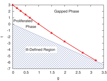
Figure 1: Phase diagram of the loop model found by numerical simulation [13]. The two phases with proliferating and small closed loops are separated by the critical line $t_{c}(g)$ drawn in red.

2.3 Surface excitations of three-dimensional topological insulators

In this section, we briefly review some aspects of the low-energy effective field theories for topological insulators and explain the relevance of the loop model in this context.

2.3.1 Bulk topological theory in $(3+1)$ dimensions

The topological insulators are characterized by time-reversal ($\cal T)$ symmetry [2]. Like other topological phases of matter they possess a bulk gap and surface massless excitations. These can have two field theory descriptions: i) in terms of free massless fermions in the case of non-interacting (band) systems [3] and ii) in terms of bosonic degrees of freedom stemming from the bulk topological gauge theory [4]. The bosonic approach is believed to be superior for modeling interacting systems.

At energies below the bulk gap, the global effects are accounted for by a topological theory. In $(3+1)$ dimensions, this is given by the so-called BF theory [4]:

$$S_{BF}[a,b,A]=i\int_{\mathcal{M}}{\dfrac{k}{2\pi}bda+\dfrac{1}{2\pi}bdA+\dfrac{\theta}{8\pi^{2}}dada}\,.$$ (2.10)

The action involves the one and two-form hydrodynamic fields $a=a_{\mu}dx^{\mu}$ and $b=(b_{\mu\nu}/2)dx^{\mu}dx^{\nu}$, that are dual to the conserved currents for vortex-line and particle bulk excitations, $V_{\mu\nu}$ and $J_{\nu}$, respectively: $V=*da$ and $J=*db$. The BF theory provides relative Aharonov-Bohm phases to these excitations. The coupling constant $k$ is a positive integer, odd (even) for fermionic (bosonic) systems, the values $k=1$ being relative to free fermions and $k>1$ to interacting systems.

The BF action includes the background gauge field $A=A_{\mu}dx^{\mu}$ and is ${\cal T}$ invariant only when the coupling $\theta\sim\theta+2\pi$ takes the values $\theta=0$ or $\theta=\pi$, the latter characterizing the nontrivial phase. By integrating out the $a$ and $b$ fields, one obtains the induced action:

$$S_{ind}[A]=i\dfrac{\theta}{8\pi^{2}k^{2}}\int_{\mathcal{M}}dAdA,\qquad\qquad\theta=\pi.$$ (2.11)

This theta term is consistent with Dirac quantization condition provided that the minimal electric charge of the system is [14]:

$$e_{0}=\frac{1}{k}\,.$$ (2.12)

This fractional value also occurs in the Aharonov-Bohm phases between bulk excitations.

The physical interesting manifolds $\mathcal{M}$ possess a boundary with dynamical surface degrees of freedom, whose action should be specified. Let us consider the expression:

$$S_{surf}[\zeta,a,A]=i\int_{\partial\mathcal{M}}d^{3}x\left(\dfrac{k}{2\pi}\varepsilon^{\mu\nu\rho}\zeta_{\mu}\partial_{\nu}a_{\rho}+\dfrac{1}{2\pi}\varepsilon^{\mu\nu\rho}\zeta_{\mu}\partial_{\nu}A_{\rho}\right)\,,$$ (2.13)

involving the boundary values of the $a,A$ fields and $\zeta=\zeta_{\mu}dx^{\mu}$, the restriction of $b$ to the boundary [4]. This action is determined by the requirement of gauge invariance of the bulk-boundary system. Actually, the complete action $S_{BF}+S_{surf}$ is invariant under $a\to a+d\lambda,b\to b+d\xi$ and $\zeta\to\zeta+\xi$.

Note that the action (2.13) does not yet include any dynamics for the surface degrees of freedom, because its Hamiltonian vanishes. Introducing a dynamics by adding terms to $S_{surf}$ will be the goal of the following discussion. However, we should first discuss the boundary conditions for quantization.

2.3.2 Solitonic modes

The three-dimensional excitations of particles and vortex-lines are sources for the $b$ and $a$ field equations of motion, respectively. Placing such excitations in the bulk determines the boundary conditions for the fields at the surface and thus introduce solitonic modes.

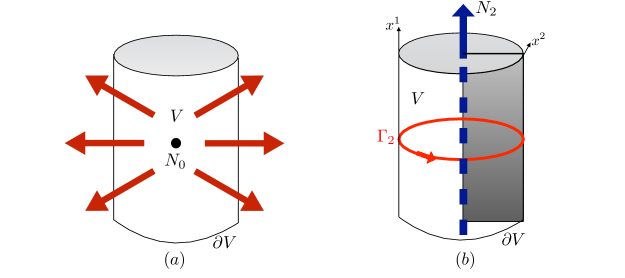
Figure 2: Relation between bulk and boundary excitations: (a) A charge $N_{0}$ in the bulk creates a flux for the $\zeta$ field on the boundary. (b) A vortex line with magnetic charge $N_{2}$ along the cycle $\Gamma_{1}$ gives a non-vanishing loop integral of the $a$ field along $\Gamma_{2}$ on the surface.

Let us consider the spatial three-dimensional geometry of the solid torus ${\cal M}=S_{1}\times S_{1}\times I$, whose boundary is the two-torus ($I$ is the interval $[0,1]$). The possible bulk excitation are summarized in Fig.2. In part (a), a static particle is put at the origin: being the source for the $b$ field, it implies a non-vanishing flux for the $\zeta$ field on the boundary torus. In part (b), a static vortex line winds along the cycle $\Gamma_{1}$ inside the solid torus: this is a source for the $a$ field, whose line integral on the cycle $\Gamma_{2}$ is non vanishing. Another condition exists by exchanging the two directions.

Therefore, the following boundary conditions are obtained for solitonic modes of the $\zeta$ and $a$ fields [15]:

$$\int_{\mathbb{T}^{2}}{d^{2}x\,\varepsilon^{ij}\partial_{i}\zeta_{j}}=\dfrac{2\pi N_{0}}{k},\quad N_{0}\in\mathbb{Z}\,,$$ (2.14)

$$\int_{\Gamma_{1}}{dx^{i}a_{i}}=\dfrac{2\pi N_{1}}{k}\,,\quad\qquad N_{1}\in\mathbb{Z}\,,$$ (2.15)

$$\int_{\Gamma_{2}}{dx^{i}a_{i}}=\dfrac{2\pi N_{2}}{k}\,,\quad\qquad N_{2}\in\mathbb{Z}\,.$$ (2.16)

2.3.3 Local surface dynamics

In earlier works [15] [16] [5], a simple dynamics for surface excitations was introduced and studied. Let us review some points of this analysis because they will be relevant for this work. The boundary action (2.13) for vanishing background, can be written in the static gauge $a_{0}=\zeta_{0}=0$ as follows,

$$S_{surf}[a,\zeta,0]=\frac{k}{2\pi}\int d^{3}x\,\varepsilon^{ij}\zeta_{i}\partial_{0}a_{j}.$$ (2.17)

This expression is the symplectic form for two pairs of canonically conjugate degrees of freedom: the first one is given by the longitudinal part $a_{i}=\partial_{i}\varphi$ and the transverse part $\zeta_{i}^{\perp}$, $\partial_{i}\zeta_{i}^{\perp}=0$; the second one involves the transverse $a_{i}^{\perp}$ and longitudinal $\zeta_{i}=\partial_{i}\lambda$ components. Disregarding the second pair, there remains the scalar field $\varphi$ and its momentum $\Pi=(k/2\pi)\varepsilon^{ij}\partial_{i}\zeta_{j}$. The simplest dynamics is obtained by adding a quadratic Hamiltonian for $\varphi$, as follows:

$$S_{surf}[\varphi]=\int d^{3}x\,\Pi\partial_{0}\varphi-\mathcal{H},\qquad\mathcal{H}=\dfrac{1}{2m}\Pi^{2}+\dfrac{m}{2}(\partial_{i}\varphi)^{2}.$$ (2.18)

The presence of the mass parameter $m$ is due to the mismatch between the original dimension of gauge fields, implying a dimensionless $\varphi$, and the standard scalar field dimension.

The boundary theory (2.18) can be written in Lagrangian form:

$$S_{surf}[\varphi]=\dfrac{m}{2}\int d^{3}x\,\partial_{\mu}\varphi\partial^{\mu}\varphi.$$ (2.19)

Furthermore, the Hamilton equations in covariant form read,

$$\dfrac{k}{2\pi}\varepsilon^{\mu\nu\rho}\partial_{\nu}\zeta_{\rho}=m\partial^{\mu}\varphi\,,$$ (2.20)

that reminds of the electric-magnetic duality in $(2+1)$ dimensions between a gauge field $\zeta$ and a dual scalar $\varphi$ [16].

The quantization of the surface theory (2.18) in presence of the solitonic modes, Eqs.(2.14-2.16), and the properties of the spectrum were obtained in the works [15] [5]. However, this theory is not completely satisfactory because it does not matches the free fermion dynamics in any limit. Let us compute the induced action in presence of the $A$ background. The coupling of $\varphi$ to $A$ is dictated by the bulk theory and amounts to the substitution $\partial_{\mu}\varphi\rightarrow\partial_{\mu}\varphi+A_{\mu}/k$. The action obtained by integrating $\varphi$ reads:

$$S_{ind}^{B}[A]=\dfrac{m}{4k^{2}}\int d^{3}xd^{3}y\,F_{\mu\nu}(x)\left(\dfrac{1}{\partial^{2}}\right)_{x,y}F^{\mu\nu}(y)\,,$$ (2.21)

using the notations introduced in Section 2.1. Note that the mass $m$ appears explicitly, and cannot be eliminated by a redefinition of the $\varphi$ field, since its coupling to $A$ is fixed.

On the other hand, the fermionic induced action can be computed by expanding the determinant to leading quadratic order in $A$, corresponding to the semiclassical, weak-field approximation. One finds [17]:

$$S_{ind}^{F}[A]=\dfrac{1}{64}\int\,F_{\mu\nu}\dfrac{1}{\partial}F^{\mu\nu}\pm\frac{1}{8\pi}\int AdA\,.$$ (2.22)

As explained in [5], the Chern-Simons term corresponding to the parity anomaly is cancelled by the bulk BF theory and should be disregarded.

We observe that the two expressions $S^{B}_{ind}$ and $S^{F}_{ind}$ differ qualitatively in the low-energy limit: the fermion theory is conformal invariant and its induced action does not include any mass scale; on the contrary, the bosonic action contains the unavoidable mass $m$. In conclusion, the local bosonic theory (2.18) describe a solvable surface dynamics that is different from that of topological band insulators. It may describe interacting fermions in a spontaneously broken phase [5].

2.3.4 Nonlocal surface dynamics and the loop model

In the earlier work [5], it was argued that a nonlocal modification of the action (2.18) could bring closer to the fermionic theory. Actually, the loop model provides the correct dynamics. Let us add its action (2.3) with couplings $(g,f)=(g_{0},0)$ to the topological term (2.13), as follows:

$$S_{surf}[a,\,\zeta,\,A]=\dfrac{i}{2\pi}\int{\left(k\zeta da+\zeta dA\right)}+\dfrac{g_{0}}{4\pi}\int a_{\mu}\left(\dfrac{-\delta_{\mu\nu}\partial^{2}+\partial_{\mu}\partial_{\nu}}{\partial}\right)a_{\nu}\,.$$ (2.23)

The integration of the field $\zeta$ implies the constraint $a=A/k$ and leads to the induced action,

$$S_{ind}[A]=\dfrac{g_{0}}{4\pi k^{2}}\int{d^{3}xd^{3}y\,\,A_{\mu}\left(\dfrac{-\delta_{\mu\nu}\partial^{2}+\partial_{\mu}\partial_{\nu}}{\partial}\right)A_{\nu}},$$ (2.24)

which reproduces the expected fermionic result (2.22) for $k=1$ and $g_{0}=\pi/8$.

Furthermore, the equation of motion for $a$ gives a nonlocal generalization of the previously seen electric-magnetic duality (2.20),

$$-i\frac{k}{2\pi}\varepsilon_{\mu\nu\rho}\partial_{\nu}\zeta_{\rho}=\dfrac{g_{0}}{2\pi}\partial\,a_{\mu}\,,$$ (2.25)

that had been heuristically suggested in [5] [16].

Therefore, the physics of topological insulators provides a strong motivation for analyzing the loop model, as it represents a viable theory for boson-fermion correspondence in the semiclassical, weak-field limits. The issue of bosonization and the meaning of the quadratic approximation will become more clear in the following sections.

Another form of the surface action is obtained by integrating out the hydrodynamic field $a_{\mu}$ in (2.23). Upon using the kernel identity (2.5), we obtain:

$$S_{surf}[\zeta,A]=\dfrac{k^{2}}{4\pi g_{0}}\int\,\zeta_{\mu}\biggr{(}\dfrac{-\delta_{\mu\nu}\partial^{2}+\partial_{\mu}\partial_{\nu}}{\partial}\biggr{)}\zeta_{\nu}+\frac{i}{2\pi}\int\,\zeta dA\,.$$ (2.26)

This again corresponds to the loop model with its coupling to the $A$ background and coupling constants:

$$g=\dfrac{k^{2}}{g_{0}},\qquad\quad f=0\,.$$ (2.27)

2.3.5 Partition function of the local theory

The partition function of the local theory (2.18) on the three torus $\mathbb{T}^{3}$ was found in Refs.[15] [5]. Let us recall its expression in the case of orthogonal axes, of spatial radii $R_{1}$ and $R_{2}$ and time period $\beta$. The canonical quantization of the $\zeta,a$ fields involves oscillator and solitonic modes satisfying the conditions (2.14-2.16). The partition function correspondingly factorizes into $Z=Z_{sol}Z_{osc}$. The first part reads:

$$Z_{sol}=\sum_{N_{0},N_{1},N_{2}\in\mathbb{Z}}{\exp{\left\{-\beta\left[\dfrac{N_{0}^{2}}{8\pi^{2}R_{1}R_{2}m}+2\pi^{2}\dfrac{m}{k^{2}}\left(N_{1}^{2}\dfrac{R_{2}}{R_{1}}+N_{2}^{2}\dfrac{R_{1}}{R_{2}}\right)\right]\right\}}}\,.$$ (2.28)

The oscillator part $Z_{osc}$ is found by zeta-function regularization of the determinant of the Euclidean Laplacian [18]. The result takes the standard form of Bose statistics times a Casimir energy term:

$$Z_{osc} = \left[\text{det}^{\prime}(-\partial^{2})\right]^{-1/2}=e^{F}\prod_{(n_{1},n_{2})\neq(0,0)}{\biggr{(}1-\exp{\biggr{(}-\dfrac{\beta}{2\pi}\sqrt{\dfrac{n_{1}^{2}}{R_{1}^{2}}+\dfrac{n_{2}^{2}}{R_{2}^{2}}}\,\,\biggr{)}}\biggr{)}^{-1}}\,,$$ (2.29)

$$F =\dfrac{\beta}{2R_{1}^{2}R_{2}^{2}}\sum_{(n_{1},n_{2})\neq(0,0)}\biggr{[}\dfrac{n_{1}^{2}}{R_{1}^{2}}+\dfrac{n_{2}^{2}}{R_{2}^{2}}\biggr{]}^{-3/2}\,,$$

where the prime indicates the exclusion of zero modes.

The expression of the partition function will be useful for checking the quantization of the loop model described in Section 3.

2.4 Duality relations in the loop model

Dualities indicate the possibility of representing a physical system with two different field theories, say by using bosonic or fermionic degrees of freedom. In (2+1) dimensions, it is well-known that non-relativistic particles can change their statistics by coupling to a Chern-Simons gauge field. Recently, this mechanism was argued to hold for relativistic theories as well, leading to several conjectures that fit into a “web of dualities” [8]. For instance, the fermion-boson duality reads [19]:

$$\mathcal{L}_{B}[\varphi]+J_{B\mu}a_{\mu}+\dfrac{i}{4\pi}ada+\dfrac{i}{2\pi}adA\sim\mathcal{L}_{F}[\psi]+J_{F\mu}A_{\mu}-\dfrac{i}{8\pi}AdA\,.$$ (2.30)

The theories on both sides of this relation are coupled to the external background field $A_{\mu}$. On the l.h.s, the bosonic current is first coupled to a dynamic Chern-Simons field that changes the statistics from bosonic to fermionic by adding a quantum of flux for each particle. On the r.h.s., the fermion parity anomaly term $(1/8\pi)AdA$ is subtracted. The duality relation is supposed to map not only kinematical quantities such as spin and charge, but also the low energy dynamics, even in the massless case. For instance, the Abelian Higgs model at the critical point is believed to be dual to a massless Dirac fermion [8]. The matter actions $\mathcal{L}_{B}[\varphi]$ and $\mathcal{L}_{F}[\psi]$ include self-interactions suitably tuned for the duality to hold.

In this context, it is interesting to analyze the loop model, in which the dualities are exact transformations, and are represented by $SL(2,\mathbb{Z})$ maps of the complex coupling constant $\tau=f+ig$.

2.4.1 Bosonic particle-vortex duality

The bosonic particle-vortex duality is schematically written as follows [19]:

$$\mathcal{L}_{B}[\phi]+j_{\mu}^{(\phi)}A_{\mu}\sim\widetilde{\mathcal{L}}_{B}[\varphi]+j_{\mu}^{(\varphi)}a_{\mu}+\dfrac{i}{2\pi}adA\,.$$ (2.31)

In this expression, on the l.h.s. the charge density $j_{0}^{(\phi)}$ of the $\phi$ field couples to the electric potential $A_{0}$: on the r.h.s., the $a_{0}$ equation of motion imply $j_{0}^{(\varphi)}\propto\varepsilon^{ij}\partial_{i}A_{j}$, meaning that the dual bosonic field $\varphi$ is magnetically charged. This fact explains the name of particle-vortex, or electric-magnetic transformation.

The partition functions of the two theories in the external background, $Z[A]$ and $\widetilde{Z}[A]$, are related by the following map:

$$Z[A]=\int\mathcal{D}a_{\mu}\,\widetilde{Z}[a]\exp{\left(\frac{i}{2\pi}\int{adA}\right)}\,.$$ (2.32)

Let us compute this transformation for the loop model (2.3) coupled the $A_{\mu}$ background, whose induced action can be found by generalizing the derivation of (2.24) in Section 2.3.4:

$$Z[A]=\exp{\left(-\frac{1}{4\pi}\int A_{\mu}D_{\mu\nu}(g,f)A_{\nu}\right)}\,.$$ (2.33)

By performing the Gaussian integral in (2.32) and using the kernel identity (2.5), we obtain that $\widetilde{Z}[A]$ takes the same form as $Z[A]$ with complex coupling constant:

$$\widetilde{\tau}=-\frac{1}{\tau}\,,\qquad\quad\tau=f+ig\,,$$ (2.34)

corresponding to the $S$ generator of the $SL(2,\mathbb{Z})$ group.

Therefore, the loop model is explicitly self-dual [1]. The physical meaning of this result will be more clear in the following, where we shall see that this theory corresponds to electrodynamics in the limit of large number of matter fields $N$.

A nice aspect of the duality transformation (2.31) is that it actually corresponds to a Legendre transformation. Let us rewrite it,

$$\widetilde{S}[{\cal J}]=S[A]-\int{\cal J}^{\mu}A_{\mu},\qquad\quad{\cal J}=\frac{1}{2\pi}*\!(da),$$ (2.35)

namely as a change of variable from the background $A$ to the “effective field” ${\cal J}$, where the new “effective potential” $\widetilde{S}[{\cal J}]\equiv\widetilde{S}[a]$ is equal to the dual action. As is well known, the second derivatives of the two potentials $S$ and $\widetilde{S}$ w.r.t. the respective variables are one the inverse of the other, $\delta^{2}S/\delta A_{1}\delta A_{2}\sim\left(\delta^{2}\widetilde{S}/\delta{\cal J}_{1}\delta{\cal J}_{2}\right)^{-1}$. The first variation w.r.t. to the background defines the induced current, while the second derivative introduces the conductivity. As a consequence, the duality implies a reciprocal relation between conductivity tensors, $\sigma_{ij}(\tau)$ and $\widetilde{\sigma}_{kn}(\widetilde{\tau})$, $i,j,k,n=1,2$, of the two theories, as follows [9]:

$$\varepsilon^{ij}\,\sigma_{jk}(\tau)\,\varepsilon^{kn}\,\widetilde{\sigma}_{nm}(\widetilde{\tau})=\frac{1}{4\pi^{2}}\delta^{i}_{m}\,.$$ (2.36)

2.4.2 Fermionic particle-vortex duality

The electric-magnetic duality for fermionic theories is conjectured to take form [19]:

$$\mathcal{L}_{F}[\psi]+j^{(\psi)}_{\mu}A_{\mu}\sim\widetilde{\mathcal{L}}_{F}[\chi]+j^{(\chi)}_{\mu}a_{\mu}+\dfrac{i}{4\pi}adA\,,$$ (2.37)

between the fermion field $\psi$ and its dual $\chi$. The map is the same as for bosonic fields (2.31) up to a normalization of the statistical field $a$.

As it will be clear in the following, the loop model describes both (the large $N$ limit of) bosonic and fermionic theories; thus, we can apply the map (2.37) to the effective action (2.33) again and obtain the relation (2.34) between the couplings up to a factor of four. Upon defining the “fermionic” version of the loop model with shifted coupling $\tau_{F}=2\tau$, we can write the fermionic duality (2.37) as:

$$\widetilde{\tau}_{F}=-\frac{1}{\tau_{F}},\qquad\quad\tau_{F}=2\tau\equiv 2\tau_{B}.$$ (2.38)

2.4.3 Boson-fermion duality

Let us now consider the transformation in Eq.(2.30): on the bosonic side, first a Chern-Simons term $ada$ is added and then the particle-vortex transformation (2.31) is applied. Acting on the loop model, these correspond to the following maps:

$$T:\tau_{B}\ \to\ \tau_{B}+1,\qquad\qquad S:\tau_{B}+1\ \to\ -\frac{1}{\tau_{B}+1}\,.$$ (2.39)

On the fermionic side, the subtraction of the anomaly term corresponds to $T^{-1}:\tau_{F}\to\tau_{F}-1$, taking into account the different normalization of the fermionic model (2.38). In conclusion, the combined map is:

$$-\frac{1}{\tau_{B}+1}=\frac{\tau_{F}-1}{2}\qquad\longrightarrow\qquad\tau_{F}=\frac{\tau_{B}-1}{\tau_{B}+1}\,.$$ (2.40)

Therefore, the loop model explicitly realizes the boson-fermion duality too.

In the literature, the dualities of Abelian theories in $(2+1)$ dimensions have been related to those of Yang-Mills theory in $(3+1)$ dimensions [20] [7]. This can be easily explained within the bulk-boundary correspondence discussed in Section 2.3: the topological bulk action (2.10) possesses the theta-term $\theta/8\pi^{2}\int dada$, that under periodicity, $\theta\to\theta+2\pi$, produces a Chern-Simons action at the boundary corresponding to the $T$ transformation $\tau_{B}\to\tau_{B}+1$ discussed above. Therefore, the dualities involving bosonic theories include the transformations $T$ and $S$ that span the $SL(2,\mathbb{Z})$ group [10].

On the other hand, the dualities within fermionic theories also belong to the $SL(2,\mathbb{Z})$ group: the transformation $S$ was found in (2.38), while $T:\tau_{F}\to\tau_{F}+1$ is obtained by integrating out one fermionic degree of freedom as in (2.22).

The boson-fermion map (2.40) can be written group theoretically as follows:

$$\tau_{F}=T\Lambda ST(\tau_{B})\,.$$ (2.41)

There appears another transformation $\Lambda:\tau_{B}\to\tau_{F}=2\tau_{B}$ that does not belong to the $SL(2,\mathbb{Z})$ group: in matrix notation, this is diagonal, $\Lambda={\rm diag}(2,1)$, with determinant two. However, this transformation cannot be iterated, i.e. $\Lambda^{n}$ does not make sense for $n\in\mathbb{Z}$, beside $n=0,\pm 1$. Thus, it is not an ordinary group element and does not enlarge the duality group.

In conclusion, dualities including both bosonic and fermionic theories belong to the group $SL(2,\mathbb{Z})$, keeping in mind the coupling normalization just discussed. In the following, we do not discuss these issues any further because we are mostly concerned with the analysis of the bosonic loop model with vanishing Chern-Simons term ($f=0$), for which the inversion $g\to 1/g$ suffices.

2.5 Electrodynamics in the large-$N$ limit and loop model

In this section, we discuss the theories of $(2+1)$-dimensional particles (both fermionic and bosonic) interacting with photons in $(2+1)$ and $(3+1)$ dimensions, corresponding to $QED_{3}$, and its mixed-dimensional modification $QED_{4,3}$ [9] [21]. We show that they reduce to the loop model in the limit of large number of matter fields.

2.5.1 Loop model and $QED_{3}$

The action of $QED_{3}$ with $N_{F}$ massless fermionic fields is,

$$S_{QED_{3}}[\psi,A]=\int{d^{3}x\,\sum_{n=1}^{N_{F}}\bar{\psi}_{n}(i\not{\partial}-\not{A})\psi_{n}}+\dfrac{1}{4e^{2}}\int{d^{3}x\,F_{\mu\nu}F_{\mu\nu}}\,.$$ (2.42)

Integration of the fermions produces the determinant of the Dirac operator raised to the $N_{F}$ power: a simplification occurs in the large $N_{F}$-limit by keeping the coupling $\lambda=e^{2}N_{F}$ finite, because the expansion of the determinant in powers of $A_{\mu}$ is dominated by the quadratic term, the higher orders being subdominant by powers of $N_{F}^{-1/2}$. The expression of the quadratic term is equal to the induced action already given in Eq.(2.22): thus, the large-$N_{F}$ limit is,

$$Z = \int{\cal D}A\,\exp\left(-S_{QED_{3}}[A]\right),$$

$$\!\!\!\!S_{QED_{3}}[A] = \dfrac{\lambda}{2}\int A_{\mu}\left(\dfrac{1}{16}\dfrac{1}{\partial}+\dfrac{1}{\lambda}\right)\left(-\delta_{\mu\nu}\partial^{2}+\partial_{\mu}\partial_{\nu}\right)A_{\nu}\,+i\frac{\eta}{8\pi}\int AdA.$$ (2.43)

The parity anomaly term has a $\pm$ sign ambiguity for each fermion component, that can be resolved by considering the limit $m\to 0^{\pm}$ of massive fields [17]. Without knowing this information or other physical input on the theory, we can only say that the parameter $\eta$ in (2.43) is an integer taking one value in the interval $-N_{F}\leq\eta\leq N_{F}$.

Next we observe that in the first part of the action (2.43), the term $1/\lambda$ involves a mass scale and is subdominant w.r.t. $1/\sqrt{k^{2}}$ in the low-energy limit. We conclude that the effective large-$N_{F}$/low-energy theory of $QED_{3}$ is described by the loop model for values of the couplings $(g,f)=(\pi/4,\eta/\lambda)$ (using the fermion normalization (2.38) and after rescaling the field $A_{\mu}\to A_{\mu}/\sqrt{\lambda}$).

2.5.2 Loop model and $QED_{4,3}$

The action of this model [9],

$$S_{QED_{4,3}}[\psi,\,A] =\int_{{\cal M}_{3}}{d^{3}x\,\sum_{n=1}^{N_{F}}\bar{\psi}(i\not{\partial}-\not{A})\psi}+\dfrac{1}{4e^{2}}\int_{{\cal M}_{4}}{d^{4}x\,F_{\mu\nu}F_{\mu\nu}}\,,$$ (2.44)

shows that the photons are defined in $(3+1)$ dimensions while the fermions live on a $(2+1)$-dimensional hyperplane. This theory is very interesting because it maps into itself under the fermionic particle-vortex duality (2.37) [9]. Let us review this result for $N_{F}=1$.

The integration of the $A_{\mu}$ field in (2.44) leads to the term $\int j^{(3)}_{\mu}(x)D^{(4)}_{\mu\nu}(x-y)j^{(3)}_{\nu}(y)$, where the three-dimensional currents interact with the four-dimensional propagator restricted to the hyperplane. We denote the coordinates as $X^{\mu}=(x^{\alpha},x^{3})$, and identify the hyperplane by $x^{3}=0$. The Green function of the four-dimensional Euclidean Laplacian $\partial^{2}_{(4)}$ on the hyperplane can be written as:

$$\left.\frac{1}{-\partial^{2}_{(4)}}(X,Y)\right|_{x^{3}=y^{3}=0}=\left.\frac{1}{4\pi^{2}}\frac{1}{(X-Y)^{2}}\right|_{x^{3}=y^{3}=0}=\frac{1}{2}\frac{1}{\partial}(x,y)\,,$$ (2.45)

i.e. it corresponds to the kernel of the loop model. Therefore, the integration of the gauge field leads to the following three-dimensional action with long-range current-current interaction:

$$S_{QED_{4,3}}[\psi]=\int_{{\cal M}_{3}}\bar{\psi}i\not{\partial}\psi+\dfrac{e^{2}}{4}\ j^{(\psi)}_{\mu}\,\dfrac{1}{\partial}\,j^{(\psi)}_{\mu}\,,$$ (2.46)

with $j_{\mu}^{(\psi)}=\bar{\psi}\gamma_{\mu}\psi$.

The dual theory with coupling constant $\widetilde{e}$ is obtained by applying the particle-vortex transformation (2.37) to (2.44):

$$\widetilde{S}_{QED_{4,3}}[\chi,a,A] =\int_{{\cal M}_{3}}{d^{3}x\,\left[\bar{\chi}(i\not{\partial}-\not{a})\chi-\dfrac{i}{4\pi}\varepsilon_{\mu\nu\rho}a_{\mu}\partial_{\nu}A_{\rho}\right]}$$

$$+\dfrac{1}{4\widetilde{e}^{2}}\int_{{\cal M}_{4}}{d^{4}x\,F_{\mu\nu}F_{\mu\nu}}\,,$$ (2.47)

where $a_{\mu}$ is the statistical field. Integration over the $A_{\mu}$ field following the same steps as before leads to the three-dimensional action:

$$\widetilde{S}_{QED_{4,3}}[\chi,a]=\int_{{\cal M}_{3}}\bar{\chi}(i\not{\partial}-\not{a})\chi+\dfrac{\widetilde{e}^{2}}{64\pi^{2}}\ a_{\mu}\biggr{(}\dfrac{-\delta_{\mu\nu}\partial^{2}+\partial_{\mu}\partial_{\nu}}{\partial}\biggr{)}a_{\nu}\,.$$ (2.48)

Finally, integrating out $a$ with the help of the loop-model identity (2.5) gives,

$$\widetilde{S}_{QED_{4,3}}[\chi]=\int_{{\cal M}_{3}}\bar{\chi}i\not{\partial}\chi+\dfrac{16\pi^{2}}{\widetilde{e}^{2}}\ j^{(\chi)}_{\mu}\,\dfrac{1}{\partial}\,j^{(\chi)}_{\mu}\,,$$ (2.49)

where $j^{(\chi)}_{\mu}=\bar{\chi}\gamma_{\mu}\chi\,$.

The comparison of the actions (2.46) and (2.49) establishes the self-duality of $QED_{4,3}$ with coupling constant relation:

$$\widetilde{e}=\dfrac{8\pi}{e}\,.$$ (2.50)

The duality implies a inverse relation between the conductivities of the two theories, as discussed in Section 2.4.1 [9]. The same results is obtained in the case of electrodynamics of scalar particles [21]; there is a difference of a factor of two in the relation (2.50), i.e. $\pi\to\pi/2$, stemming from the duality transformations (2.31) and (2.37).

Let us now discuss the large $N_{F}$-limit of $QED_{4,3}$. It is convenient to start from the dual action (2.48): the integration over the fermions yields again the $N_{F}$ power of the determinant and its quadratic approximation holds for $N_{F}\to\infty$ and $\lambda=e^{2}N_{F}$ fixed, as in the case of $QED_{3}$. We obtain the action:

$$S_{QED_{4,3}}[a]=\biggr{(}\dfrac{1}{32}+\dfrac{1}{\lambda}\biggr{)}\int\,a_{\mu}\biggr{(}\dfrac{-\delta_{\mu\nu}\partial^{2}+\partial_{\mu}\partial_{\nu}}{\partial}\biggr{)}a_{\nu}\,+\,i\frac{\eta}{8\pi\lambda}\int ada\,,$$ (2.51)

after rescaling of $a_{\mu}\to a_{\mu}/\sqrt{\lambda}$.

We conclude that $QED_{4,3}$ in the large $N_{F}$-limit is equivalent to the fermionic loop model (2.3) with coupling constant:

$$g=\pi\left(\dfrac{1}{4}+\dfrac{8}{\lambda}\right)\,.$$ (2.52)

This result is very important because it establishes that the loop model is the limit of a viable theory of interacting electrons: for example, on the surface of three-dimensional topological insulators discussed in Section 2.3, the higher-dimensional photons can be physical and not merely a technical advantage. In the next Section we shall see that the relation with $QED_{4,3}$ also provides a physical approach to quantize the loop model.

We conclude this section by adding some remarks:

• Eq. (2.52) shows that the dimensionless coupling constant $\lambda>0$ of $QED_{4,3}$ remap the critical line $g>1$ of the loop model. Note that $QED_{3}$ is found at the point $\lambda=\infty$ on this line.

• It is believed that $QED_{4,3}$ possesses a critical line also for finite $N_{F}$ [22], that then spans $e^{2}<8\pi$ owing to the self-duality (2.50). Note, however, that the finite-$N_{F}$ self-duality does not survive the large $N_{F}$ limit and is replaced by the loop model duality at $N_{F}=\infty$.

• Finally, the analysis of scalar $QED_{4,3}$ in the large $N_{B}$ limit reproduces again the loop model up to numerical factors in the coupling constant relation (2.52). Indeed, the quadratic expansion of the bosonic determinant has the same expression of the fermionic theory, but without the anomalous Chern-Simons term.

3 Quantization of the loop model on $\mathbb{T}^{3}$

In this section we analyze the surface excitations of topological insulators with loop-model dynamics, as discussed in Section 2.3.4. We recall the expression of the action (2.23):

$$S_{surf}[a,\,\zeta,\,0]=\dfrac{ik}{2\pi}\int\zeta da+\dfrac{g_{0}}{4\pi}\int a_{\mu}\left(\dfrac{-\delta_{\mu\nu}\partial^{2}+\partial_{\mu}\partial_{\nu}}{\partial}\right)a_{\nu}\,,$$ (3.1)

where the $A$ background has been switched off and the anomalous Chern-Simons term is cancelled by the bulk, so as to respect time-reversal symmetry (coupling $f=0)$. We consider the bulk geometry of the solid torus $\mathbb{T}^{3}\times I$. The nontrivial part of the surface dynamics is given by the solitonic excitations that are defined by the boundary conditions of the $\zeta$ and $a$ fields in (2.14-2.16), corresponding to global magnetic and electric fluxes on the spatial torus $\mathbb{T}^{2}$.

In addition, the compactness of the $a$ field allows for further magnetic solitons. We place ourselves in the massless phase of the loop model where local monopoles are suppressed but global fluxes are possible on compact geometries. The corresponding condition reads:

$$\int_{\mathbb{T}^{2}}{\varepsilon^{ij}\partial_{i}a_{j}}=\dfrac{2\pi}{q_{0}}M_{0},\qquad\qquad M_{0}\in\mathbb{Z}\,,$$ (3.2)

where $q_{0}$ is the minimal charge for the $a$ field.

The usual method of quantization is based on expanding the fields in solitonic and oscillator parts and evaluate the partition function in terms of classical action and fluctuations around it. This analysis is not possible for the nonlocal theory (3.1) that does not have a Hamiltonian formulation and is not well defined on-shell.

This problem can be solved by reformulating the loop model as a local theory in $(3+1)$ dimensions, as we now explain. We take some inspiration from the mixed-dimension $QED_{4,3}$, where photons live in $(3+1)$ dimensions and are coupled to a current confined to a $(2+1)$-dimensional hyperplane. As seen in the previous section, integration of the photons yields the nonlocal loop model interaction on the surface.

We introduce an extra dimension and define the following action:

$$S_{4}[\hat{a},\zeta]=\dfrac{1}{4e^{2}}\int_{\mathcal{M}_{4}}d^{4}x\,\left(\partial_{\mu}\hat{a}_{\nu}-\partial_{\nu}\hat{a}_{\mu}\right)^{2}+i\dfrac{k}{2\pi}\int_{\mathcal{M}_{3}}{ad\zeta}\,.$$ (3.3)

In this expression, the four-dimensional manifold is $\mathcal{M}_{4}=\mathbb{T}^{3}\times\mathbb{R}$ with extra coordinate $x_{3}\in\mathbb{R}$, $\hat{a}_{\mu}$ is the four-dimensional extension of the field $a_{\mu}$ on $\mathcal{M}_{3}=\mathbb{T}^{3}$ and $e$ is a coupling constant to be determined later. The three-dimensional part of the action (3.3) can be written as a source term,

$$i\int_{\mathcal{M}_{4}}J^{\mu}\hat{a}_{\mu}\,,\qquad\qquad J_{\alpha}=\delta(\mathcal{M}_{3})\dfrac{k}{2\pi}\varepsilon_{\alpha\beta\gamma}\partial_{\beta}\zeta_{\gamma}\,,\qquad J_{3}=0,$$ (3.4)

where $\delta{(\mathcal{M}_{3})}=\delta(x_{3})$ is the delta function on the hyperplane. The spatial part of this geometry is drawn in Fig.3.

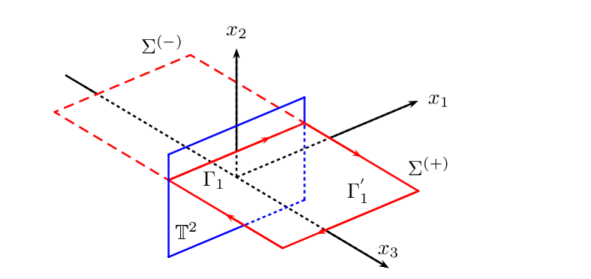
Figure 3: Three-dimensional extension of the spatial torus $\mathbb{T}^{2}$. The torus is drawn in blue, while the surfaces $\Sigma^{(+)}$ and $\Sigma^{(-)}$ are in red.

The $(3+1)$-dimensional action (3.3) corresponds to ordinary electrodynamics that is well defined on-shell. We can compute its partition function by decomposing the fields $\hat{a}$ and $\zeta$ into solitonic and oscillator parts:

$$Z=\sum_{sol\ config}e^{-S_{4}[\hat{a}_{sol},\zeta_{sol}]}\int{\mathcal{D}\hat{a}_{osc}\,\mathcal{D}\zeta_{osc}e^{-S_{4}[\hat{a}_{osc},\zeta_{osc}]}}\,,$$ (3.5)

where $\hat{a}_{sol}$ are classical solutions of the $(3+1)$-dimensional equations of motion obeying the $(2+1)$-dimensional boundary conditions for the $a,\zeta$ fields (2.14-2.16) and (3.2).

Next the integration of wave modes of the field $\hat{a}$ in $S_{4}[\hat{a}_{osc},\zeta_{osc}]$, following usual steps, leads to the $(2+1)$-dimensional action for (the wave modes of) $\zeta_{\mu}$:

$$S[\zeta]=\dfrac{k^{2}e^{2}}{16\pi^{2}}\int\zeta_{\mu}\biggr{(}\dfrac{-\delta_{\mu\nu}\partial^{2}+\partial_{\mu}\partial_{\nu}}{\partial}\biggr{)}\zeta_{\nu}\,.$$ (3.6)

This expression is the same as the that of the original surface action $S_{surf}[a,\zeta]$ (2.23), after eliminating the $a$ field (cf. Section 2.3.4, Eq.(2.26)), leading to the coupling identification:

$$e^{2}=\frac{4\pi}{g_{0}}.$$ (3.7)

In conclusion, the loop model (2.23) has been transformed into the local theory in $(3+1)$ dimensions (3.3), that allows for a proper definition and calculation of solitonic modes.

3.1 Evaluation of solitonic modes

The $(3+1)$-dimensional Minkowskian action for static solitonic configuration $S_{4}[\hat{a}_{sol},\zeta_{sol}]$ corresponds to the Hamiltonian,

$$S_{4}[\hat{a}_{sol},\zeta_{sol}]=-\beta\,H,\qquad H=\dfrac{1}{2e^{2}}\int{d^{3}x\left(\boldsymbol{B}^{2}+\boldsymbol{E}^{2}\right)}\,,$$ (3.8)

involving the electric and magnetic fields $\boldsymbol{E}$ and $\boldsymbol{B}$ of $\hat{a}_{\mu}$. The integration is done on the spatial part of $\mathcal{M}_{4}$ (cf. Fig.3), specified by the torus periods, $\boldsymbol{\omega}_{1}=(0,2\pi R_{1},0)$ and $\boldsymbol{\omega}_{2}=(0,0,2\pi R_{2})$, and by a finite interval, $x_{3}\in[-1/(2M),1/(2M)]$, for the extra coordinate, where $1/M$ is the infrared cutoff to be discussed later.

Let us now solve the $\hat{a}_{\mu}$ equations of motion with source term (3.4). The magnetic flux configuration for $\zeta_{\mu}$ on $\mathbb{T}^{2}$ (2.14) determines a constant current $J_{0}$ on the $x_{3}=0$ plane, which is coupled to $\hat{a}_{0}$ by the Poisson equation:

$$\nabla^{2}\hat{a}_{0}=-e^{2}J_{0}\,,\qquad J_{0}=\delta(x_{3})\frac{N_{0}}{V^{(2)}},\qquad V^{(2)}=4\pi^{2}R_{1}R_{2}\,.$$ (3.9)

The solution $\hat{a}_{0}=\hat{a}_{0}(x_{3})$ is easily found and it determines the electric field component along $x_{3}$:

$$E_{3}=-\dfrac{d}{dx_{3}}\hat{a}_{0}=\dfrac{e^{2}N_{0}}{2V^{(2)}}\text{sign}(x_{3})\,.$$ (3.10)

The contribution of the electric field to the Hamiltonian (3.8) is obtained by integrating over three-space, with the result:

$$H_{el}=\dfrac{e^{2}N_{0}^{2}}{32\pi^{2}R_{1}R_{2}M}\,.$$ (3.11)

Next we consider the configurations of electric flux for $a$ on the $x^{3}=0$ plane (2.15), given by the line integral on $\Gamma_{1}$. This can be extended to a close circuit on the edge of the surface $\Sigma^{(+)}$ (cf. Fig.3); two sides of this contour cancel each other and the contribution $\Gamma_{1}^{\prime}$ at large $x_{3}$ vanishes by assumption. Thus, the $a$ line integral can be rewritten as the flux of the magnetic field $B_{2}$ through $\Sigma^{(+)}$, leading to:

$$B_{2}=\dfrac{2M}{k}\dfrac{N_{1}}{R_{1}}\text{sign}(x_{3})\,.$$ (3.12)

In this expression, the sign function appears for the possible exchange of $\Sigma^{(+)}$ with $\Sigma^{(-)}$. In analogous fashion, the other flux condition (2.16) determines a magnetic field along $x_{1}$:

$$B_{1}=\dfrac{2M}{k}\dfrac{N_{2}}{R_{2}}\text{sign}(x_{3})\,.$$ (3.13)

Finally, the magnetic flux configuration for $a$ (3.2) on the $x^{3}=0$ plane is reproduced by the following $x_{3}$-independent field component:

$$B_{3}=\dfrac{M_{0}}{q_{0}2\pi R_{1}R_{2}}\,.$$ (3.14)

The total magnetic contribution to the energy is then found to be:

$$H_{mag}=\frac{M_{0}^{2}}{4\pi e^{2}q_{0}^{2}MR_{1}R_{2}}+\dfrac{8\pi^{2}M}{e^{2}k^{2}}\left(N_{1}^{2}\dfrac{R_{2}}{R_{1}}+N_{2}^{2}\dfrac{R_{1}}{R_{2}}\right)\,.$$ (3.15)

From the evaluation of the classical solutions we thus obtain the following expression of the solitonic part of the partition function of the loop model on $\mathbb{T}^{3}$:

$$\!\!Z_{sol}=\!\!\sum_{N_{\mu},M_{0}\in\mathbb{Z}}\exp\left\{-\beta\left[\dfrac{2\pi g_{0}M}{k^{2}}\left(N_{1}^{2}\dfrac{R_{2}}{R_{1}}+N_{2}^{2}\dfrac{R_{1}}{R_{2}}\right)+\frac{1}{R_{1}R_{2}M}\left(\frac{N_{0}^{2}}{8\pi g_{0}}+\frac{M_{0}^{2}g_{0}}{16\pi^{2}q_{0}^{2}}\right)\right]\right\},$$ (3.16)

where we substituted the coupling $g_{0}$ using (3.7). Let us complete the calculation of the partition function before discussing this result.

3.2 Oscillator modes

The partition function of the oscillator modes can be obtained from the nonlocal $(2+1)$-dimensional Lagrangian (3.6) by computing the determinant of the positive definite Euclidean Laplacian. Choosing the Lorentz gauge, the spectral decomposition reads:

$$S=\dfrac{k^{2}}{4\pi g_{0}}\sum_{n_{\alpha}\in\mathbb{Z}^{3}\neq(0,0,0)}\zeta_{\mu}(n)\sqrt{\left(k_{n}\right)^{2}}\zeta_{\nu}(n)\,,$$ (3.17)

where $k^{\mu}_{n}$ are the discretized momenta on $\mathbb{T}^{3}$. The field $\zeta$ possesses two physical polarizations, instead of one for local Yang-Mills theory. Thus, the oscillator part of the partition function is given by the determinant,

$$Z_{osc}=\left[\text{det}^{\prime}\left(\sqrt{-\partial^{2}}\right)\right]^{-1}=\left[\text{det}^{\prime}\left(-\partial^{2}\right)\right]^{-1/2}\,.$$ (3.18)

As a matter of fact, this oscillator partition function is equal to that of the local bosonic theory (2.19), discussed in Section 2.3.5. We remark that $Z_{osc}$ is independent of the coupling constant.

In conclusion, the partition function of the loop model on $\mathbb{T}^{3}$ is given by $Z=Z_{sol}Z_{osc}$, where the expressions of $Z_{sol}$ and $Z_{osc}$ are given in (3.16) and (2.29), respectively.

3.3 Interpolating theory and the choice of infrared cut-off

The torus partition function found in the previous section possesses striking similarities with the corresponding quantity in the local scalar theory of surface excitations discussed in Section 2.3.3. The oscillator part take the same form; regarding the solitonic sum, let us compare the expression (3.16) with the analogous one of the scalar theory (2.28), reported in Section 2.3.5. We see that the terms parameterized by $N_{0},N_{1},N_{2}$ remarkably match in the two formulas, upon identifying the respective mass parameters by $m=Mg_{0}/\pi$. On the other hand, the $M_{0}$ term for $a$ magnetic solitons is absent in the scalar theory, because the latter corresponds to the longitudinal part of the gauge field, $a_{\mu}=\partial_{\mu}\varphi$ (cf. Section 2.3.3)

This remarkable equivalence can be explained as follows: the two theories are different, but can be matched on-shell. For example, the off-shell induced actions $S_{ind}[A]$ (2.21) and (2.24) are unequal, and this fact originally motivated the study of the nonlocal theory.

In order to understand these results, we reformulate the loop model by introducing the infrared cutoff as an explicit photon mass $\widetilde{M}$. The modification of the action (3.1) reads:

$$S_{m}=i\frac{k}{2\pi}\int\zeta da+\frac{g_{0}}{4\pi}\int a_{\mu}\left(\frac{\delta_{\mu\nu}(-\partial^{2}+\widetilde{M}^{2})+\partial_{\mu}\partial_{\nu}}{\sqrt{-\partial^{2}+\widetilde{M}^{2}}}\right)a_{\nu}\,.$$ (3.19)

In the Lorentz gauge, this becomes:

$$S_{m}[a,\zeta]=\dfrac{ik}{2\pi}\int{\zeta da}+\dfrac{g_{0}}{4\pi}\int{d^{3}x\,d^{3}y\,a_{\mu}\sqrt{-\partial^{2}+\widetilde{M}^{2}}\,a_{\mu}}\,.$$ (3.20)

Upon integrating on $a$, this action describes conserved currents with cutoffed long-range interaction: $\int J_{\mu}(1/\partial)J_{\mu}\to\int J_{\mu}(1/\sqrt{-\partial^{2}+\widetilde{M}^{2}})J_{\mu}$. Therefore, $S_{m}$ can be considered as an equivalent formulation of the loop model, where the cutoff is explicit and not added a-posteriori in the classical field solutions.

Let us now analyze the theory on-shell: the equations of motion for $a$,

$$-i\dfrac{k}{2\pi}\varepsilon_{\mu\nu\rho}\partial_{\nu}\zeta_{\rho}=\dfrac{g_{0}}{2\pi}\sqrt{-\partial^{2}+\widetilde{M}^{2}}a_{\mu}\rightarrow\begin{cases}&\dfrac{g_{0}}{2\pi}\partial a_{\mu}\,,\quad\text{UV}\,,\\ \\ &\dfrac{g_{0}}{2\pi}\widetilde{M}a_{\mu}\,,\quad\text{IR}\,,\end{cases}$$ (3.21)

interpolate between those of the nonlocal and local theories, Eqs. (2.20) and (2.25). The equation of motion for $\zeta_{\mu}$ imposes $a_{\mu}=\partial_{\mu}\varphi$: substituting in $S_{m}$, we find the reduced action,

$$S_{m}=\dfrac{\widetilde{M}g_{0}}{4\pi}\int{d^{3}x\,\partial_{\mu}\varphi\partial_{\mu}\varphi}\,,\qquad\qquad\text{(on-shell)}\,.$$ (3.22)

Therefore, the massive nonlocal action $S_{m}$ (3.19) is equal to the local action (2.19) on-shell (up to a numerical factor). This implies that the two theories have same solitonic spectra and partition functions. On the other hand, the $S_{m}$ (3.19) spectrum is also equal to that of the loop model in Section 3.1, up to a parameter change, because they correspond to different choices of cut-off in the same theory. These facts explain the matching of $Z_{sol}$ for the local and nonlocal theories, Eqs. (2.28) and (3.16) (for $M_{0}=0$).

Two conclusions can be drawn from this analysis:

• The on-shell correspondence provides a check for the calculation of soliton configurations through the $(3+1)$-dimensional extension of the the loop model.

• The IR regularization of the loop model with a fixed mass parameter $M$ violates scale invariance at the quantum level, in disagreement with the fermionic dynamics. Therefore, another choice of cutoff is needed.

Let us consider the cutoff given by the spatial dimension of the system, namely replace:

$$M\ \longrightarrow\ \frac{1}{\sqrt{R_{1}R_{2}}},$$ (3.23)

in the expressions of Section 3.1

Within this choice, the solitonic partition function $Z_{sol}$ (3.16) of the loop model becomes:

$$Z_{sol}=\sum_{N_{0},N_{1},N_{2},M_{0}\in\mathbb{Z}}\exp\biggr{\{}-\beta\dfrac{1}{\sqrt{R_{1}R_{2}}}\biggr{[}\dfrac{2\pi g_{0}}{k^{2}}\left(N_{1}^{2}\dfrac{R_{2}}{R_{1}}+N_{2}^{2}\dfrac{R_{1}}{R_{2}}\right)+\dfrac{N_{0}^{2}}{8\pi g_{0}}+\dfrac{M_{0}^{2}g_{0}}{16\pi^{2}q_{0}^{2}}\biggr{]}\biggr{\}}\,.$$ (3.24)

This expression is manifestly scale invariant and also invariant under $R_{1}\Leftrightarrow R_{2}$.

Let us remark that the choices of “geometric cutoff” in (3.24) and “fixed cutoff” in (3.16) and (3.19) actually amount to two different definitions of the nonlocal theory at the quantum level. In the following we adopt the first choice realizing a scale invariant theory. Further justifications will arise in the study of the partition function on the $S^{2}\times\mathbb{R}$ geometry.

4 Quantization on the cylinder $S^{2}\times\mathbb{R}$

In this section, we compute the partition function for the manifold $S^{2}\times\mathbb{R}$, made by a spatial sphere and Euclidean time. As is well-known, this geometry can be mapped to flat space by the conformal transformation $r=R\exp(u/R)$, where $r$ is the radius of $\mathbb{R}^{3}$ and $u$ is Euclidean time on the cylinder. It follows that time evolution on the cylinder corresponds to dilatations in $\mathbb{R}^{3}$ and the energy spectrum gives access to conformal dimensions of the fields in the theory [10] [18]. The partition function is schematically:

$$Z\sim\sum_{\Delta}\,\exp\left(-\beta\frac{v\Delta}{R}\right),$$ (4.1)

where $\Delta$ are the conformal dimensions and $v$ is the Fermi velocity.

The computation of the partition function will follow the same steps as in the previous section by using the four-dimensional formulation. We consider the manifold $\mathcal{M}_{4}=S^{3}\times\mathbb{R}$ and embed the three-dimensional space $\mathcal{M}_{3}=S^{2}\times\mathbb{R}$ by identifying $S^{2}$ with the equator of $S^{3}$.

The four-dimensional Minkowskian action (3.3) on $\mathcal{M}_{4}=S^{3}\times\mathbb{R}$ takes the form:

$$S_{4}[\hat{a},\zeta]=-\dfrac{1}{4e^{2}}\int_{\mathcal{M}_{4}}{dx\,\sqrt{-g}g^{\mu\alpha}g^{\nu\beta}\hat{f}_{\mu\nu}\hat{f}_{\alpha\beta}}+\dfrac{k}{2\pi}\int_{\mathcal{M}_{3}}{ad\zeta}\,.$$ (4.2)

This action is conformal invariant at the classical level: four-dimensional transformations may induce a nontrivial metric on ${\cal M}_{3}$, but this is ineffective on the Chern-Simons action. Our strategy will be that of assuming conformal invariance in the quantum theory and then check it in the results (using the IR cutoff compatible with dilatations).

4.1 Solitonic modes on $S^{2}$ embedded in $S^{3}$

The four-dimensional manifold $S^{3}\times\mathbb{R}$ is described by the metric $ds^{2}=dt^{2}-R^{2}d\Omega_{3}^{2}$, in terms of $S^{3}$ polar coordinates, $d\Omega_{3}^{2}=\sin^{2}\psi(d\theta^{2}+\sin^{2}\theta d\varphi^{2})$, with $\psi,\theta\in[0,\pi]$ and $\varphi\in[0,2\pi]$. The $S^{2}$ sphere at the equator is identified by $\psi=\pi/2$.

On the geometry of the sphere, there exist global magnetic fluxes for the $a$ and $\zeta$ fields. These obey, as in (2.14) and (3.2),

$$\int_{S^{2}}{da}=\dfrac{2\pi}{q_{0}}M_{0}\,,\qquad\quad M_{0}\in\mathbb{Z},$$ (4.3)

$$\int_{S^{2}}{d\zeta}=\dfrac{2\pi}{k}N_{0}\,,\qquad\quad N_{0}\in\mathbb{Z}.$$ (4.4)

The electric fluxes for the $a$ field are instead absent because cycles on $S^{2}$ are topologically trivial.

Following the same steps as in the previous section, we solve the equations of motion for the action (4.2), with source term localized on ${\cal M}_{3}$. This can be rewritten:

$$\frac{k}{2\pi}\int_{{\cal M}_{4}}\delta(\mathcal{M}_{3})\,ad\zeta,\qquad\delta(\mathcal{M}_{3})=\dfrac{\delta(\psi-\pi/2)}{R\sin^{2}(\psi)}\,.$$ (4.5)

Note that the form of the delta function is covariant under translations along the $\psi$ coordinate, i.e. displacements of $S^{2}$ from the equator of $S^{3}$.

The $\zeta$ magnetic flux (4.4) amounts to a “charge density” located at $\psi=\pi/2$ coupled to $\hat{a}_{0}$ by the Poisson equation,

$$\nabla_{\mu}\nabla^{\mu}\hat{a}_{0}=-\dfrac{e^{2}N_{0}}{4\pi R^{2}}\dfrac{\delta(\psi-\pi/2)}{R\sin^{2}(\psi)}\,.$$ (4.6)

In this equation, it is natural to assume that $\hat{a}_{0}$ depends only on $\psi$, and thus the covariant Laplacian reduces to an ordinary differential equation. The solution is easily found to be:

$$\hat{a}_{0}(\alpha)=\dfrac{e^{2}N_{0}}{8\pi R}\left|\tan(\alpha)\right|\,,\qquad\quad\alpha=\psi-\frac{\pi}{2}\,.$$ (4.7)

The other solitonic solution (4.3) is a magnetic flux for the $a$ field that is orthogonal to $S^{2}$ and can be chosen to be a constant for all $\psi$ values, i.e. all embeddings $S^{2}\subset S^{3}$:

$$B_{\psi}(\psi)=\hat{f}_{\theta\varphi}(\psi)=\dfrac{M_{0}}{2q_{0}}\frac{1}{R^{2}\sin^{2}(\psi)}\,.$$ (4.8)

We now compute the energies associated to the two solitonic solutions (4.7), (4.8). The Hamiltonian is given by,

$$H=\dfrac{1}{2e^{2}}\int_{S^{3}}{d^{3}x\,\sqrt{g}\left[\hat{f}_{i0}\hat{f}_{j0}g^{ij}+\dfrac{1}{2}\hat{f}_{ij}\hat{f}_{lk}g^{il}g^{jk}\right]}\,,$$ (4.9)

where we recognize the electric and magnetic parts. The electric contribution is obtained by inserting the solution (4.7) for $\hat{f}_{\psi 0}=\partial_{\psi}\hat{a}_{0}$:

$$H_{el}=\dfrac{1}{2e^{2}}\int_{S^{3}}d^{3}x\,\sqrt{g}\,g^{\psi\psi}\left(\partial_{\psi}\hat{a}_{0}\right)^{2}=\dfrac{N_{0}e^{2}}{32\pi R}\int_{-\pi/2}^{\pi/2}d\alpha\dfrac{1}{\cos^{2}(\alpha)}\,.$$ (4.10)

This integral is divergent at the two poles of $S^{3}$, $\alpha=\pm\pi/2$: an infrared cutoff is again needed. Let us first introduce a fixed scale, by setting a maximal “length” $|R\tan(\alpha)|<1/(2M)$: we obtain the result,

$$H_{el}=\dfrac{N_{0}^{2}}{8g_{0}R}\left(\dfrac{1}{MR}\right),$$ (4.11)

in terms of the loop model coupling $g_{0}$ given by (3.7).

The magnetic energy is similarly computed from the solution (4.8):

$$H_{mag}=\dfrac{1}{2e^{2}}\int_{S^{3}}d^{3}x\,\sqrt{g}\left(\hat{f}_{\theta\varphi}g^{\theta\varphi}\right)^{2}=\dfrac{M_{0}^{2}g_{0}}{8q_{0}^{2}R}\int_{-\pi/2+\delta}^{\pi/2-\delta}d\alpha\dfrac{1}{cos^{2}(\alpha)}\,.$$ (4.12)

This is the same divergent integral of the electric contribution: once regularized, it yields:

$$H_{mag}=\dfrac{M_{0}^{2}g_{0}}{8q_{0}^{2}R}\left(\dfrac{1}{MR}\right).$$ (4.13)

The values of the classical energies (4.10), (4.13) determine the solitonic part of the partition function on the geometry $S^{1}\times S^{2}$:

$$Z_{sol}=\sum_{N_{0},M_{0}\in\mathbb{Z}}\exp\left\{-\frac{\beta}{R}\left(\dfrac{1}{8MR}\right)\left[\frac{N_{0}^{2}}{g_{0}}+\frac{g_{0}M_{0}^{2}}{q_{0}^{2}}\right]\right\}\,.$$ (4.14)

We note again that the fixed cutoff $M$ is incompatible with scale invariance. In analogy with the torus case, we replace this scale with the system dimension, $M=1/(8\lambda R)$ with $\lambda$ a numerical constant. We thus obtain:

$$Z_{sol}=\sum_{N_{0},M_{0}\in\mathbb{Z}}\exp\left\{-\frac{\beta\lambda}{R}\left[\frac{N_{0}^{2}}{g_{0}}+g_{0}\frac{M_{0}^{2}}{q_{0}^{2}}\right]\right\}\,.$$ (4.15)

The form of $Z_{sol}$ is now in agreement with conformal invariance, Eq. (4.1), and the free parameter $\lambda$ enters in the definition of the non-universal Fermi velocity. The expression (4.15) is an important result of our work: we shall analyze it after completing the derivation of partition function.

4.2 Oscillator spectrum

The oscillator part $Z_{osc}$ is obtained from the Euclidean $(2+1)$-dimensional action (3.6), by evaluating the determinant of the nonlocal kernel. The action can be rewritten in the form (for $\partial_{\mu}\zeta^{\mu}=0)$:

$$S[\zeta]=\frac{k^{2}}{2\pi g_{0}}\int_{\mathbb{R}_{3}}\zeta_{\mu}(x_{1})\frac{\delta^{\mu\nu}}{(x_{1}-x_{2})^{4}}\zeta_{\nu}(x_{2})\,.$$ (4.16)

Under the conformal map $r=R\exp(u/R)$ from $\mathbb{R}^{3}$ to ${\cal M}_{3}=\mathbb{R}\times S^{2}$, with respective coordinates $x^{\mu}=(r,\theta,\varphi)$ and $\widetilde{x}^{\alpha}=(u,\theta,\varphi)$, the action is covariant,

$$S[\zeta]=\frac{k^{2}}{2\pi g_{0}}\int_{{\cal M}_{3}}d^{3}\widetilde{x}_{1}d^{3}\widetilde{x}_{2}\sqrt{g(\widetilde{x}_{1})g(\widetilde{x}_{2})}\ \widetilde{\zeta}_{\alpha}(\widetilde{x}_{1})\left(\frac{e^{2(u_{1}+u_{2})/R}}{(x_{1}-x_{2})^{4}}\right)g^{\alpha\beta}\,\widetilde{\zeta}_{\beta}(\widetilde{x}_{2}),$$ (4.17)

where the transformations are [18], $b_{\mu}dx^{\mu}=\widetilde{b}_{\alpha}d\widetilde{x}^{\alpha}$, $g^{\alpha\beta}=\delta^{\alpha\beta}e^{(u_{1}+u_{2})/R}$, and the expression in parenthesis is the correlator of scalar conformal fields with dimension $\Delta=2$ on the cylinder. Note that the expression (4.17) is conformal invariant but not reparameterization invariant.

The first step in the calculation of the determinant is that of finding the eigenvalues: these are obtained by the spectral decomposition of the $1/x^{4}$ correlator in the covariant basis of the cylinder, i.e. Fourier modes $\exp(i\omega u)$ and spherical harmonics $Y_{\ell}^{m}(\theta,\varphi)$. Next, the determinant is obtained by zeta-function regularization of the product of eigenvalues [18]. This rather long calculation is done in Appendix B: here we report the main steps.

The spectral decomposition reads:

$$\frac{e^{2(u_{1}+u_{2})/R}}{(x_{1}-x_{2})^{4}}=\frac{8}{R^{4}}\sum_{\ell=0}^{\infty}\sum_{m=-\ell}^{m=\ell}\int_{\infty}^{\infty}d\omega\,e^{i\omega(u_{1}-u_{2})}\,Y_{\ell}^{m}(\theta_{1},\varphi_{1})\,\lambda_{\omega,\ell}\,Y^{m*}_{\ell}(\theta_{2},\varphi_{2}),$$ (4.18)

where the eigenvalues are,

$$\lambda_{\omega,\ell}=\sum_{k=0}^{\infty}\frac{2k+\ell+2}{(\omega R)^{2}+(2k+\ell+2)^{2}}\frac{\Gamma(k+3/2)\Gamma(k+\ell+2)}{\Gamma(k+\ell+3/2)\Gamma(k+1)}\,.$$ (4.19)

The sum in this expression is ultraviolet divergent because $1/x^{4}$ is not a proper distribution. Rather surprisingly, it can be evaluated, with result:

$$\lambda_{\omega,\ell}=\left(\sum_{k=0}^{\infty}\frac{1}{2}\right)+\frac{\ell+1}{4}-\frac{\pi}{4}\left|\frac{\Gamma\left((\ell+2+i\omega R)/2\right)}{\Gamma\left((\ell+1+i\omega R)/2\right)}\right|^{2}\,.$$ (4.20)

The first two terms in this expression, respectively divergent and finite, correspond to functions with support for $x_{1}=x_{2}$ only, that are subtracted for defining the renormalized $1/x^{4}$ kernel.

The product of eigenvalues can be simplified by using an infinite-product representation of the Gamma function; dropping inessential factors, one finds:

$$\prod_{n\in\mathbb{Z},\ \ell\geq 0}\lambda_{n,\ell}\propto\prod_{n\in\mathbb{Z},\ \ell\geq 0}\widehat{\lambda}_{n,\ell}\,,\qquad\quad\widehat{\lambda}_{n,\ell}=\left(\frac{2\pi nR}{\beta}\right)^{2}+\Lambda_{\ell},$$ (4.21)

where $\lambda_{n,\ell}=\lambda_{\omega,\ell}$ for discretized momentum $\omega=2\pi n/\beta$ on $S^{1}$ and $\Lambda_{\ell}$ refer to angular momentum. The eigenvalues $\widehat{\lambda}_{n,\ell}$ have now the standard form of Laplace-type operators on the geometry $S^{1}\times S^{2}$.

The regularization of the determinant is obtained by introducing the zeta-function:

$$\zeta_{S^{1}\times S^{2}}(s)=\sum_{\ell=\ell_{min}}^{\infty}\sum_{n\in\mathbb{Z}}\frac{\delta(\ell)}{(\widehat{\lambda}_{n,\ell})^{s}},$$ (4.22)

where $\delta(\ell)$ is the multiplicity of eigenvalues. The analytic continuation from large positive values of ${\rm Re}(s)$ to $s\sim 0$ leads to the following expression of the partition function [18],

$$Z_{osc}=\exp\left\{\left.\frac{1}{2}\frac{d}{ds}\zeta_{S^{1}\times S^{2}}(s)\right|_{s=0}\right\}=e^{-\beta{\cal C}/R}\prod_{\ell=\ell_{min}}^{\infty}\left[1-\exp{\left(-\frac{\beta\sqrt{\Lambda_{\ell}}}{R}\right)}\right]^{-\delta(\ell)}\,,$$ (4.23)

where the Casimir energy ${\cal C}/2R$ is obtained by evaluating the further zeta-function,

$${\cal C}=\zeta_{S^{2}}\left(-1/2\right)\,,\qquad\quad\zeta_{S^{2}}(s)=\sum_{\ell=\ell_{min}}^{\infty}\frac{\delta(\ell)}{\Lambda^{s}_{\ell}}.$$ (4.24)

The resulting partition function for the loop model takes the form (4.23) with parameters $({\cal C},\sqrt{\Lambda_{l}},\delta(\ell),\ell_{min})$ given in the first line of Table 1. The results of other quadratic theories are also reported in this Table for the following discussion.

5 Conformal invariance and spectrum of the loop model

In this section, we discuss some interesting informations on the spectrum that can be drawn from the expression of $Z=Z_{sol}Z_{osc}$ on $S^{1}\times S^{2}$.

5.1 Particle-vortex duality

The solitonic spectrum in $Z_{sol}$ given by (4.15) involves “electric” and “magnetic” quantum numbers $N_{0}$ and $M_{0}$, respectively. In the fermionic case, corresponding to $k=1$ and minimal charge $q_{0}=1$, the spectrum is manifestly invariant for $g_{0}\rightarrow 1/g_{0}$. This self-duality is expected, because the conformal fields characterize many observables of the theory and should occur in self-dual pairs.

On the other hand, the solitonic spectrum on the torus $\mathbb{T}^{3}$, given by (3.16) is not self-dual, even for vanishing electric fluxes $N_{1}=N_{2}=0$. Actually, the $(2+1)$-dimensional duality is not a symmetry of the partition function, but a Legendre transformation, as explained in Section 2.4.1. This cannot be verified in our expressions of $Z$ with vanishing $A$ background: one would need to extend the derivation for constant $A$, compute the conductivities and check that they obey the reciprocity relation (2.36).

5.2 Conformal invariance

The conformal invariance of the loop model is rather natural in the $(3+1)$-dimensional formulation (3.3), as discussed in Section 4, but is not obvious in the nonlocal form in $(2+1)$ dimensions (3.1). The quantization procedure has actually shown that scale invariance of the solitonic spectrum is only realized by using a proper IR cutoff. The oscillator part $Z_{osc}$ (4.23) provides further evidences of conformal invariance at the quantum level:

• In a conformal theory, the Casimir energy on $S^{2}\times\mathbb{R}$ is related to the trace anomaly, that vanishes in $(2+1)$ dimensions [18]. The result ${\cal C}=0$ (cf. Table 1) matches this expectation, as non-zero values would have implied non-anomalous classical terms in the trace of the stress tensor.

• The integer-spaced dimensions of descendent (derivative) fields is also apparent by the fact that $\sqrt{\Lambda_{\ell}}\in\mathbb{Z}$ in Table 1. For example, the spectrum of non-conformal local Yang-Mills theory $(2+1)$ dimensions, also reported in the Table, does not have this property: thus, energies do not correspond to scale dimensions, i.e. the theory is not covariant under the conformal map to the plane.

5.3 Comparison with other theories

The loop model corresponds to the large $N$ limit of mixed-dimension $QED_{4,3}$: it has a quadratic action but is not a free theory. The inclusion of solitonic modes makes it an interesting conformal theory, that is similar to the compactified boson theory in $(1+1)$ dimensions. The results for the partition function of some free conformal theories reported in Table 1 provide other elements for this discussion.

The data indicate that the spectrum of descendent fields is integer as in $(3+1)$-dimensional theories, while the conformal scalar in $(2+1)$ dimensions starts from $\Delta_{\varphi}=1/2$. On the other hand, the multiplicities $\delta(\ell)$ are linear in $\ell$ as in $(2+1)$ dimensions, instead of being quadratic, a characteristic feature of angular momentum on $S^{3}$.

Going back to the $(3+1)$-dimensional action (3.3) and integrating over the $\zeta$ field, one find that the loop model can be seen as a constrained Yang-Mills theory, enjoying a subspace of its Hilbert space. The comparison between the first and last lines of Table 1 shows this fact. In conclusion, the loop model is a conformal theory with mixed-dimension properties, whose features would need a deeper analysis using representation theory of the conformal group.

$$\begin{array}[]{|l|c|c|c|c|c|}\hline\cr{\rm Theory}&{\rm dimension}&{\cal C}&\sqrt{\Lambda_{\ell}}&\delta(\ell)&\ell_{min}\\ \hline\cr{\rm loop\ model}&(2+1)&0&\ell&2\ell&1\\ {\rm conformal\ scalar}&(2+1)&0&\ell+\frac{1}{2}&2\ell+1&0\\ {\rm vector}&(2+1)&\neq 0&\sqrt{\ell(\ell+1)}&2\ell+1&1\\ {\rm conformal\ scalar}&(3+1)&\frac{1}{120}&\ell&\ell^{2}&1\\ {\rm vector}&(3+1)&\frac{3}{20}&\ell&2(\ell^{2}-1)&2\\ \hline\cr\end{array}$$

Table 1: Parameters entering in the partition function (4.23) of some quadratic theories [18]: Casimir energy $\cal C$; energy level $\sqrt{\Lambda}_{\ell}$; eigenvalue degeneracy $\delta(\ell)$; minimal value $\ell_{min}$

.

5.4 Anyon excitations

Let us analyze the results of Section 4 for $k>1$, that are relevant for the dynamics at the surface of interacting topological insulators (cf. Section 2.3). In this case, the partition function (4.14) should describe excitations with fractional charge and statistics in $(2+1)$ dimensions. The subject is well understood for non-relativistic dynamics, as e.g. in the fractional quantum Hall effect. The loop model provides a description in the relativistic scale-invariant domain.

The form of the surface action (2.23) in Section 2.3.4,

$$S_{surf}[a,\zeta,A]=\frac{i}{2\pi}\int\left(k\zeta da+\zeta dA\right)+S_{loop}[a],$$ (5.1)

tells us that:

• The $\zeta$ field is dual to the background $A$ with minimal charge $e_{0}=1/k$, Eq. (2.12); thus, magnetic excitations of $\zeta$ possess minimal charge $\widetilde{e}_{0}=1/k$ in agreement with the quantization condition (2.14).

• The $a$ field is dual to $\zeta$, i.e. it is electric, and possesses minimal charge $q_{0}=1$, as confirmed by the constraint $A\sim k\,a$ implemented by $\zeta$. Therefore, its monopoles have minimal charge one for any $k$ value (cf. Eq.(3.2) for $q_{0}=1$).

• The map between the actions (2.23) and (2.26), i.e. by integrating the $a$ field, is a generalization of the particle-vortex duality transformation for theories with fractional charges (cf. Section 2.4.1). In this transformation, the loop-model coupling is mapped into:

  $$\widetilde{g}_{0}\equiv g=\frac{k^{2}}{g_{0}}.$$ (5.2)

These results lead us to consider the solitonic spectrum (4.15) at the electric-magnetic self-dual point $g_{0}=k$:

$$E_{sol}=\frac{v}{R}\Delta_{N_{0},M_{0}}\,,\qquad\Delta_{N_{0},M_{0}}=\frac{1}{2}\left[\frac{N_{0}^{2}}{k}+kM_{0}^{2}\right],\qquad\quad(g_{0}=k).$$ (5.3)

Upon writing $N_{0}=kn+m$, with $m=0,1,\dots,k-1$ and $n\in\mathbb{Z}$, this spectrum contains states with fractional dimensions $\Delta=m^{2}/(2k)+\mathbb{Z}$. Thus, there are $k$ independent anyonic sectors in agreement with the value $k$ of the topological order on the $S^{2}\times S^{1}$ geometry (this can be computed from the bulk BF theory, as explained e.g. in Section 3.3.1 of Ref.[5]).

Furthermore, the behaviour of conformal correlators on the surface of topological insulators should match the known Aharonov-Bohm phases between excitations predicted by the BF theory (2.10),

$$\theta=\frac{2\pi n_{1}n_{2}}{k},\qquad\quad n_{1},n_{2}\in\mathbb{Z}\,.$$ (5.4)

Let us explain this point in some detail.

As nicely discussed in Ref.[23], order-disorder fields in $(2+1)$ dimensions require: i) gauge fields and ii) a symplectic structure. Given the equal-time commutation relations,

$$\left[a_{i}(x,t),\pi^{j}(y,t)\right]=i\delta_{i}^{j}\delta^{(2)}(x-y),\qquad\quad i,j=1,2,$$ (5.5)

between the gauge field $a$ and its conjugate momentum $\pi$, the order and disorder operators take the form, respectively,

$$\sigma(x,t) = \exp\left(-i\alpha\int_{-\infty}^{x}d\xi^{i}a_{i}(\xi,t)\right),$$

$$\mu(x,t) = \exp\left(i\beta\int_{-\infty}^{x}d\xi^{i}\varepsilon_{ij}\pi^{j}(\xi,t)\right),$$ (5.6)

where the line integrals go to $-\infty$ along a given common direction, e.g. the negative real axis. Upon using the identity $\varepsilon^{ij}\partial_{i}\partial_{j}{\rm Arg}(x-y)=\pi\delta^{(2)}(x-y)$, one finds the (equal-time) monodromy:

$$\mu\left(e^{i2\pi}z,t\right)\sigma(0,t)=e^{i2\alpha\beta}\,\mu(z,t)\sigma(0,t),\qquad\qquad z=x_{1}+ix_{2}\,.$$ (5.7)

This topological information is contained in the part $\int k\,\zeta da$ of the action (5.1), where the canonical momentum is $\pi^{i}=k/(2\pi)\varepsilon^{ij}\zeta_{j}$, as explained in Section 2.3.3. Therefore, exponentials of line integrals (5.6) of the $a$ and $\zeta$ fields realize the expected monodromies (5.4) at the surface of the topological insulators, by suitably choosing the $\alpha,\beta$ parameters.

The dynamics introduced by $S_{loop}$ in (5.1) yields two-point functions of conformal fields, $\langle\phi(x)\phi(0)\rangle=(x^{2})^{\Delta}$. Evaluated at equal time, $x_{\mu}=(0,x_{1},x_{2})$, the power-law behavior $|z|^{2\Delta}$ should match the monodromy phase (5.4) for reconstructing the analytic dependence $z^{2\Delta}$ of conformal invariance in the two-dimensional plane. The values of $\Delta$ in the spectrum (5.3) do verify this requirement.

In conclusion, the loop model action (2.23) describes the surface excitations of fractional topological insulators for the self-dual value of the coupling constant $g=k$. The identification of the conformal spectrum (5.3) also requires a choice of Fermi velocity $v$.

We remark that the $(1+1)$-dimensional chiral boson theory describing topological insulators in one lower dimension also involves some tuning of parameters [24] [10]. Note also that the $(1+1)$-dimensional conformal spectrum,

$$\Delta_{n,\overline{n},m}=\frac{1}{4k}\left[\left(k(n+\overline{n})+2m\right)^{2}+\left(k(n-\overline{n})\right)^{2}\right],$$ (5.8)

cannot be written in the form (5.3) for odd $k$. Actually, the $(1+1)$-dimensional theory involves pairing of chiral-antichiral excitations for respecting time-reversal symmetry, while each $(2+1)$-dimensional excitation is symmetric.

6 Conclusions

In this paper, we have shown that the loop model is a conformal theory in $(2+1)$ dimensions that bears some similarities with the compactified boson in $(1+1)$ dimensions [10]. Its coupling constant spans a critical line along which the spectrum displays fermionic and anyonic excitations, thus providing a viable approach towards bosonization of free and interacting fermions. The formulation as a local theory in $(3+1)$ dimensions allows for other interesting developments.

Let us mention possible extensions of our work:

• The generalization of the analysis in presence of the Chern-Simons interaction (coupling $f\neq 0$ in (1.1)) will provide a dyonic spectrum that breaks parity and time-reversal symmetry and is covariant under more general duality transformations [25].

• The analysis of order-disorder fields can be extended beyond the simple observations of Section 5.4. In this respect, we note that in the $(2+1)$-dimensional formulation (3.1), one gauge field is non-dynamic or can be integrated out, Eq. (2.26). Thus, either the order or the disorder fields should become collective excitations.

• The loop model can be made interacting by including $1/N_{F}$ corrections stemming from the relation with $QED_{4,3}$. In this respect, it provides a viable platform for quantitative discussions of the dualities and other interesting aspects of $(2+1)$-dimensional physics.

• Finally, the $(3+1)$ local formulation of the theory can be useful for studying non-Abelian generalizations.

Acknowledgments

We would like to thank Z. Komargodski, N. Magnoli, E. Marino, C. Morais-Smith, G. Palumbo, D. Seminara and P. Wiegmann for very useful scientific exchanges. We also acknowledge the hospitality and support by the Simons Center for Geometry and Physics, Stony Brook, Nordita, Stockholm, and the G. Galilei Institute for Theoretical Physics, Arcetri. This work is supported in part by the Italian Ministery of Education, University and Research under the grant PRIN 2017 “Low-dimensional quantum systems: theory, experiments and simulations.”

Appendix A Peierls argument

We evaluate the Euclidean action of the loop model (2.6) on the configuration of a monopole with minimal magnetic charge $2\pi/q_{0}$:

$$F_{\mu\nu}=\dfrac{1}{2q_{0}}\varepsilon_{\mu\nu\rho}\dfrac{x_{\rho}}{|x|^{3}}\,.$$ (A.1)

The integral of the nonlocal term in (2.6) reads:

$$S = \dfrac{g}{32\pi^{3}q_{0}^{2}}\int{\dfrac{d^{3}x_{1}}{|x_{1}|^{3}}\,\dfrac{d^{3}x_{2}}{|x_{2}|^{3}}\,\dfrac{(x_{1}\cdot x_{2})}{|x_{1}-x_{2}|^{2}}}$$ (A.2)

$$= \dfrac{g}{4\pi q_{0}^{2}}\int_{0}^{\infty}d\alpha\int_{0}^{\infty}{dr_{1}}\int_{0}^{\infty}{dr_{2}}\int_{-1}^{1}{dy\,}y\,e^{-\alpha({r_{1}^{2}+r_{2}^{2}-2r_{1}r_{2}y})}\,,$$

where we have used polar coordinates, exponentiated the denominator and introduced the variable $y=\cos(\theta_{1}-\theta_{2})$. Upon rescaling the radii, $s_{i}=r_{i}\sqrt{\alpha}$, $i=1,2$, the integral factorizes into a logarithmic divergent part and a finite part, namely the integrals over $\alpha$ and over the others variables.

We observe that being $\alpha$ conjugated to $r^{2}$, we can regularize the divergent contribution as follows:

$$\int_{0}^{+\infty}\dfrac{d\alpha}{\alpha}\quad\rightarrow\quad\int_{1/L^{2}}^{1/a^{2}}\dfrac{d\alpha}{\alpha}=2\ln\biggr{(}\dfrac{L}{a}\biggr{)}\,,$$ (A.3)

where $\alpha$ and $L$ are the lattice constant and the system size respectively. On the other hand the finite part can be evaluated in polar coordinates $s_{1}=s\cos(\eta)$, $s_{2}=s\sin(\eta)$, leading to the result (2.8).

Appendix B Loop-model determinant on $S^{2}\times\mathbb{R}$

In this appendix we give some details concerning the calculation of the oscillator spectrum and determinant of the loop model reported in Section 4.2. The first step is the spectral decomposition of the $1/x^{4}$ kernel in the action (4.16).

B.1 Kernel decomposition

As a warming up, we determine the spectral form of the propagator of scalar fields,

$$\langle\phi(x_{1})\phi(x_{2})\rangle_{\mathbb{R}^{3}}=\dfrac{1}{|{x_{1}-x_{2}}|}.$$ (B.1)

The conformal map from flat space $x^{\mu}=(r,\theta,\varphi)$ to the cylinder $\widetilde{x}^{\alpha}=(u,\theta,\varphi)$ is obtained by transforming the fields, $\widetilde{\phi}=e^{u/2R}\phi$, leading to:

$$\langle\widetilde{\phi}(\widetilde{x}_{1})\widetilde{\phi}(\widetilde{x}_{2})\rangle_{\mathbb{R}\times S^{2}}=\frac{e^{(u_{1}+u_{2})/2R}}{|x_{1}-x_{2}|}.$$ (B.2)

This expression can be expanded in terms of Legendre polynomials $P_{\ell}$ and spherical harmonics $Y_{\ell}^{m}$, by using [26]:

$$\frac{1}{|x_{1}-x_{2}|} = \sum_{\ell=0}^{\infty}\dfrac{r_{1}^{\ell}}{r_{2}^{\ell+1}}P_{\ell}\left(\widehat{x}_{1}\cdot\widehat{x}_{2}\right),\qquad\quad x_{i}=r_{i}\widehat{x}_{i},\ \ i=1,2,\ \ r_{1}<r_{2},$$

$$P_{\ell}\left(\widehat{x}_{1}\cdot\widehat{x}_{2}\right) = \frac{4\pi}{2\ell+1}\sum_{m=-\ell}^{\ell}Y_{\ell}^{m\,*}\left(\theta_{1},\varphi_{1}\right)Y_{\ell}^{m}\left(\theta_{2},\varphi_{2}\right)\,.$$ (B.3)

Introducing the Fourier modes $e^{i\omega u}$, we obtain the spectral decomposition:

$$\langle\widetilde{\phi}(x_{1})\widetilde{\phi}(x_{2})\rangle_{\mathbb{R}\times S^{2}} =4\pi\int_{-\infty}^{\infty}d\omega\,\sum_{\ell=0}^{\infty}\sum_{m=-\ell}^{\ell}e^{i\omega(u_{1}-u_{2})}\,Y_{\ell}^{m\,*}\left(\theta_{1},\varphi_{1}\right)\,\lambda_{\omega,\ell}\,Y_{\ell}^{m}\left(\theta_{2},\varphi_{2}\right)\,,$$ (B.4)

$$\lambda_{\omega,\ell} =\dfrac{1}{\left(R\omega\right)^{2}+\left(\ell+1/2\right)^{2}}.$$

This spectrum confirms that the propagator is the inverse of the conformal Laplacian in $(2+1)$ dimensions, as reported in Table 1 for the conformal scalar theory.

Let us now apply the same procedure to the $1/x^{4}$ kernel. We use the identity,

$$\dfrac{1}{|x|^{4}}=\dfrac{1}{2|x|}\int_{0}^{\infty}dp\,p^{2}\,e^{-p|x|},$$ (B.5)

and the formula:

$$\dfrac{e^{-p|x_{1}-x_{2}|}}{|x_{1}-x_{2}|}=\sum_{\ell=0}^{\infty}\dfrac{\left(2\ell+1\right)}{\sqrt{r_{1}r_{2}}}I_{\ell+\frac{1}{2}}\left(pr_{1}\right)K_{\ell+\frac{1}{2}}\left(pr_{2}\right)P_{\ell}\left(\widehat{x}_{1}\cdot\widehat{x}_{2}\right),\qquad\quad r_{1}<r_{2},$$ (B.6)

where $I_{m}$ and $K_{m}$ are modified Bessel functions of the first and second kind, respectively. The integration over $p$ of the Bessel functions leads to the Hypergeometric function ${{}_{2}F_{1}}$; the kernel with appropriated Weyl factors is then written:

$$\dfrac{e^{2\left(u_{1}+u_{2}\right)/R}}{|x_{1}-x_{2}|^{4}}=\dfrac{\sqrt{\pi}}{R^{4}}\sum_{\ell=0}^{\infty}e^{-|u|(\ell+2)/R}\dfrac{\Gamma\left(\ell+2\right)}{\Gamma\left(\ell+\frac{1}{2}\right)}\,{{}_{2}F_{1}}\left(\dfrac{3}{2},\ell+2,\ell+\frac{3}{2};e^{-2|u|}\right)P_{\ell}\left(\widehat{x}_{2}\cdot\widehat{x}_{2}\right),$$ (B.7)

where $u=u_{1}-u_{2}$. Finally, the series expansion of the Hypergeometric function allows one to compute the Fourier modes, leading to the spectral decomposition (4.18) with eigenvalues (4.19):

$$\lambda_{\omega,\ell}=\sum_{k=0}^{\infty}\frac{2k+\ell+2}{(\omega R)^{2}+(2k+\ell+2)^{2}}\frac{\Gamma(k+3/2)\Gamma(k+\ell+2)}{\Gamma(k+\ell+3/2)\Gamma(k+1)}\,.$$ (B.8)

B.2 Field decomposition

The spin-one field on the cylinder $\widetilde{\zeta}$ is expanded in the basis of vector spherical harmonics ${\rm Y}^{JLSM}_{\mu}$, with $S=1$, that can be written in terms of scalar harmonics $Y^{m}_{L}$ and constant vectors $\chi_{\mu}^{m}$ by using the addition of angular momenta [26]:

$$\widetilde{\zeta}_{\mu}\left(\widetilde{x}\right) =\int\dfrac{d\omega}{2\pi}\,e^{i\omega u}\sum_{J=1}^{\infty}\sum_{L=J-1}^{J+1}\sum_{M=-J}^{J}\widetilde{\zeta}_{J,L,M}\left(\omega\right){\rm Y}_{\mu}^{JL1M}\left(\theta,\varphi\right)\,,$$ (B.9)

$${\rm Y}_{\mu}^{JL1M}\left(\theta,\varphi\right) =\sum_{m=-L}^{L}\sum_{m^{\prime}=-1}^{1}C_{L,1}\left(J,M,m,m^{\prime}\right)Y_{L}^{m}\left(\theta,\varphi\right)\chi_{\mu}^{m^{\prime}},$$

where $C_{L,1}\left(J,M,m,m^{\prime}\right)$ are the Clebsh-Gordan coefficients with $M=m+m^{\prime}$.

Upon substituting the previous expansions in the Euclidean action (4.16) and making use of orthonormality, we obtain:

$$S[\zeta]\propto\int\dfrac{d\omega}{2\pi}\,\sum_{L=0}^{\infty}\sum_{J=L-1}^{L+1}\sum_{M=-J}^{J}\left|\widetilde{\zeta}_{J,L,M}\left(\omega\right)\right|^{2}\,\lambda_{\omega,L}\,,$$ (B.10)

where $\widetilde{\zeta}_{-1,L,M}\left(\omega\right)=0$. The eigenvalues $\lambda_{\omega,L}$ (B.8) of the scalar kernel (B.7) only depends on the orbital momentum and reduce the summations in (B.10) to a single one over $L=0,1,\dots$, with multiplicities $\delta(L)$. The gauge condition $\partial^{\mu}\zeta_{\mu}=0$ imposes $\widetilde{\zeta}_{L,L,M}(\omega)=0$, and one finds,

$$\delta(L)=2\left(2L+1\right)\,.$$ (B.11)

B.3 Resummation and regularization

The sum over $k$ in the eigenvalues $\lambda_{\omega,\ell}$ (B.8) is regularized by subtracting the asymptotic $k\to\infty$ limit of the summand, equal to $1/2$:

$$I\left(\ell\right)=\sum_{k=0}^{\infty}\left[\dfrac{\left(\ell+2+2k\right)}{a^{2}+\left(\ell+2+2k\right)^{2}}\dfrac{\Gamma\left(\ell+2+k\right)\Gamma\left(k+3/2\right)}{\Gamma\left(\ell+3/2+k\right)\Gamma\left(k+1\right)}-\dfrac{1}{2}\right],$$ (B.12)

where $a=\omega R$. The series (B.12) can be summed by using the Sommerfeld-Watson method and the result is expressed in terms of two finite products for even and odd $\ell$ values, respectively:

$$I\left(\ell\right)=\dfrac{\ell+1}{4}-\begin{cases}&\ \qquad\dfrac{\pi a}{8}\displaystyle{\prod_{i=0}^{\left(\ell-1\right)/2}}\dfrac{\left(2i+1\right)^{2}+a^{2}}{\left(2i\right)^{2}+a^{2}}\tanh\left(\dfrac{a\pi}{2}\right)\,,\quad\ell=1,3,\dots\,,\\ \\ &\displaystyle{\frac{\pi(1+a^{2})}{8a}\prod_{i=0}^{\ell/2}}\dfrac{\left(2i\right)^{2}+a^{2}}{\left(2i-1\right)^{2}+a^{2}}\coth\left(\dfrac{a\pi}{2}\right)\,,\quad\ell=0,2,\dots\,.\end{cases}$$ (B.13)

Both products are rewritten as a ratio of complex gamma functions squared, leading to the regularized eigenvalues,

$$\lambda_{\omega,\ell}^{reg}=I\left(\ell\right)-\dfrac{\ell+1}{4}=-\dfrac{\pi}{4}\left|\frac{\Gamma\left((\ell+2+i\omega R)/2\right)}{\Gamma\left((\ell+1+i\omega R)/2\right)}\right|^{2}\,,$$ (B.14)

reported in (4.20). For compact time $\beta$, the Fourier modes are discretized, $\omega R=n/\tau$, with $\tau=\beta/(2\pi R)$, $n\in\mathbb{Z}$.

Next, the infinite-product representation of the gamma function [27],

$$\frac{\Gamma\left(a+ib\right)}{\Gamma\left(a\right)}=e^{-i\gamma b}\left(1+i\frac{b}{a}\right)^{-1}\prod_{k=1}^{\infty}e^{ib/k}\left(1+i\frac{b}{a+k}\right)^{-1},\qquad\quad a,b\in\mathbb{R},$$ (B.15)

is used to rewrite the product of eigenvalues occurring in the determinant. Dropping inessential $\tau$-independent factors, we obtain the expression:

$$\sum_{n,\ell}\delta(\ell)\log\left(\lambda_{n,\ell}^{reg}\right) = \sum_{n\in\mathbb{Z}}\sum_{\ell,k=0}^{\infty}\delta(\ell)\log\left[\dfrac{n^{2}+\tau^{2}(\ell+2k+1)^{2}}{n^{2}+\tau^{2}(\ell+2k+2)^{2}}\right]$$ (B.16)

$$= \sum_{n\in\mathbb{Z}}\sum_{L=0}^{\infty}2L\log\left(n^{2}+\tau^{2}L^{2}\right)\,.$$

The sums in this expression simplify because the indices $\ell$ and $k$ come in the combination $L=\ell+2k$. The resulting sum over $n,L$, with multiplicity $\delta(L)=2L$, can now be analytically continued by using the zeta-function method, as described in the main text.

References

- [1] E. Fradkin, S. Kivelson, “Modular invariance, self-duality and the phase transition between quantum Hall plateaus”, Nucl. Phys. B 474, 543 (1996); H. Goldman, E. Fradkin, “Loop models, modular invariance, and three-dimensional bosonization”, Phys. Rev. B 97, 195112 (2018).
- [2] E. H. Fradkin, “Field Theories of Condensed Matter Physics,” II edition, Cambridge Univ. Press, Cambridge (2013).
- [3] B. A. Bernevig, T. L. Hughes, “Topological Insulators and Topological Superconductors”, Princeton Univ. Press, Princeton (2013).
- [4] X. L. Qi, T. Hughes, S. C. Zhang, “Topological Field Theory of Time-Reversal Invariant Insulators,” Phys. Rev. B 78 (2008) 195424; G. Y. Cho, J. E. Moore, “Topological BF field theory description of topological insulators,” Annals Phys. 326 (2011) 1515.
- [5] A. Cappelli, E. Randellini, J. Sisti, “Three-dimensional topological insulators and bosonization", JHEP 2017, 135 (2017).
- [6] A. Chan, T. L. Hughes, S. Ryu, E. Fradkin, “Effective field theories for topological insulators by functional bosonization,” Phys. Rev. B 87 (2013) 085132; A. P. O. Chan, T. Kvorning, S. Ryu, E. Fradkin, “Effective hydrodynamic field theory and condensation picture of topological insulators,” Phys. Rev. B 93 (2016) 155122.
- [7] D. T. Son, “Is the Composite Fermion a Dirac Particle?,” Phys. Rev. X 5 (2015) 031027; C. Wang, T. Senthil, “Dual Dirac liquid on the surface of the electron topological insulator”, Phys. Rev. X 5, 041031 (2015); N. Seiberg, T. Senthil, C. Wang, E. Witten, “A Duality Web in 2+1 Dimensions and Condensed Matter Physics,” Annals Phys. 374 (2016) 395; M. A. Metlitski, A. Vishwanath, “Particle-vortex duality of two-dimensional Dirac fermion from electric-magnetic duality of three-dimensional topological insulators,” Phys. Rev. B 93 (2016) 245151.
- [8] T.Senthil, D. T. Son, C. Wang, C. Xue, “Duality between -d quantum critical points”, Phys. Rep. 827 (2019) 1; C. Turner, “Lectures on Dualities in 2+1 Dimensions,” arXiv:1905.12656.
- [9] W.-H. Hsiao, D. T. Son, “Duality and universal transport in mixed-dimension electrodynamics", Phys. Rev. B 96, 075127 (2017).
- [10] P. Di Francesco, P. Mathieu, D. Sénéchal, Conformal Field Theory, Springer-Verlag, New York (1997).
- [11] J. B. Kogut, “An Introduction to Lattice Gauge Theory and Spin Systems,” Rev. Mod. Phys. 51 (1979) 659.
- [12] A. M. Polyakov, “Quark Confinement and Topology of Gauge Groups,” Nucl. Phys. B 120 (1977) 429.
- [13] S. D. Geraedts, O. I. Motrunich, “Line of continuous phase transitions in a three-dimensional U(1) loop model with current-current interactions”, Phys. Rev. B 85, 144303 (2012).
- [14] P. Ye, M. Cheng, E. Fradkin, “Fractional S-duality, classification of fractional topological insulators and surface topological order”, Phys. Rev. B 96, 085125 (2017).
- [15] C.T. Hsieh, G. Y. Cho, S. Ryu, “Global anomalies on the surface of fermionic symmetry-protected topological phases in (3+1) dimensions”, Phys. Rev. B 93 (2016) 075135; X. Chen, A. Tiwari, S. Ryu, “Bulk-boundary correspondence in (3+1)-dimensional topological phases,” Phys. Rev. B 94 (2016) 045113.
- [16] A. Amoretti, A. Blasi, N. Maggiore, N. Magnoli, “Three-dimensional dynamics of four-dimensional topological BF theory with boundary,” New J. Phys. 14 (2012) 113014.
- [17] A. N. Redlich, “Parity Violation and Gauge Noninvariance of the Effective Gauge Field Action in Three-Dimensions” Phys. Rev. D 29 (1984) 2366; A. J. Niemi, G. W. Semenoff, “Axial Anomaly Induced Fermion Fractionization and Effective Gauge Theory Actions in Odd Dimensional Space-Times,” Phys. Rev. Lett. 51 (1983) 2077.
- [18] A. Cappelli, A. Coste, “On the Stress Tensor of Conformal Field Theories in Higher Dimensions,” Nucl. Phys. B 314 (1989) 707; A. Cappelli, G. D’Appollonio, “On the trace anomaly as a measure of degrees of freedom,” Phys. Lett. B 487 (2000) 87.
- [19] A. Karch, D. Tong, “Particle-Vortex Duality from 3d Bosonization,” Phys. Rev. X 6 (2016) 031043; A. Karch, B. Robinson, D. Tong, “More Abelian Dualities in 2+1 Dimensions,” JHEP 1701 (2017) 017.
- [20] E. Witten, “On S duality in Abelian gauge theory,” Selecta Math. 1 (1995) 383.
- [21] W.-H. Hsiao, D. T. Son, “Self-Dual Bosonic Quantum Hall State in Mixed Dimensional QED”, Phys. Rev. B 100, 235150 (2019).
- [22] D. Dudal, A. J. Mizher, P. Pais, “Exact quantum scale invariance of three-dimensional reduced QED theories”, Phys. Rev. D 99, 045017 (2019).
- [23] E. C. Marino, Quantum Field Theory Approach to Condensed Matter Physics, Cambridge Univ. Press, Cambridge (2017).
- [24] A. Cappelli, G. V. Dunne, C. A. Trugenberger and G. R. Zemba, “Conformal symmetry and universal properties of quantum Hall states,” Nucl. Phys. B 398 (1993) 531.
- [25] L. Di Pietro, D. Gaiotto, E. Lauria, J. Wu, “3d Abelian Gauge Theories at the Boundary,” JHEP 1905 (2019) 091.
- [26] A. Messiah, Quantum Mechanics Vol. I, Dover Publ., New York (2014); J. M. Blatt, V. F. Weisskopf, Theoretical Nuclear Physics, Dover Publ., New York (2010).
- [27] H. Bateman, Higher Transcendental Functions, Vol.I, McGraw-Hill Book Company, New York (1953).