Entangled baryons: violation of Inequalities based on local realism assuming dependence of decays on hidden variables

Abstract

Bell inequalities are consequences of local realism while violated by quantum mechanics. In particle physics, entangled high energy particles can be produced from a common source, and the decay of each particle plays the role of measurement. However, in a hidden variable theory, the decay could be determined by hidden variables. This loophole killed such approaches to Bell test in particle physics. It is a special form of measurement-setting or free-will loophole, which also exists in other systems. Using entangled baryons, we present new inequalities of local realism with the explicit assumption of the dependence of the decays on hidden variables, as well as the consideration of the statistical mixture of polarizations and the separation of local hidden variables for objects with spacelike distances. These violations closes the measurement-setting loophole once and for all. We propose to use the processes $\eta_{c}\to\Lambda\bar{\Lambda}$ and $\chi_{c0}\to\Lambda\bar{\Lambda}$ to test our inequalities, and show that their violations are likely to be observed with the data already collected in BESIII.

1 Introduction

Entanglement in particle physics was noticed long ago 1960s , and has since been studied theoretically and experimentally EntangledMesonTheoryAndExp . The entangled pseudoscalar mesons are very useful in studying violations of the discrete symmetries DoubleTag ; CPT , especially the time reversal symmetry TViolation . Moreover, many endeavours have been made to test Bell’s inequalities (BI) BI ; chsh using entangled mesons MesonBI and baryons BaryonBI ; MomemtumRepresentation . For these entangled high energy particles, mostly the quantum mechanical measurement of each particle is effectively achieved through its decay, which is not a free choice of the experimentalist. Therefore, in a realistic or hidden variable theory, the decay could depend on hidden variables at the creation of the entangled pairs, leading to the violation of BI. In the derivation of BI, however, it is assumed that the decay does not depend on hidden variables. Therefore, BI implemented in terms of decays of these entangled high energy particles cannot serve to distinguish local realistic theories from quantum mechanics.

Previously it has been noted that an experiment using decay time as the effective measurement basis cannot serve as as a genuine test of BI HEPLoopholeDiscussions . We emphasize that in a realistic theory, any kind of effective measurement accomplished through the decay could be determined by the hidden variables. This is actually a special form of the so-called measurement-setting for free-will loophole, well known in other systems FreeWillLoophole .

Recently, we made the dependence of the measurement setting on hidden variables an explicit assumption in deriving a new Leggett inequality (LI) MesonLeggett , which is a consequence of the so-called crypto-nonlocal realism LI ; LINature , and showed its violation in entangled mesons MesonLeggett . Violation of LI demonstrates that it is not enough to make the realism even cryotp-nonlocal.

In this paper, in terms of entangled hyperons, a kind of baryons, we present a new kind of inequalities, which are consequences of local realism. But it is different from BI, as it is considered that a physical state is a statistical mixture of subensembles with definite values of observables, and that the local hidden variables are separated for objects with spacelike distances, including copies of the same ones from the past when their light cones overlap. In particular, we take into account that the possibility that the signals, as the effective measurement settings, also depend on hidden variables. Hence our approach closes the measurement setting loopholes once and for all. Our inequalities are neither LIs, though inspired by them, as we consider local realism, rather than nonlocal realism.

Specifically our inequalities are constructed for the entangled $\Lambda\bar{\Lambda}$ pairs created in decays of the charmonia $\eta_{c}$ and $\chi_{c0}$, which are mesons consisting of charm quark $c$ and its antiparticle $\bar{c}$. We estimate the significances of the violations of our inequities, and find that the violations are likely to be observed with the data sample collected in BESIII at the Beijing Electron-Position Collider II.

Our proposal demonstrates that the entangled baryon pairs provide a new playground of entanglement study in the realm of particle physics, for relativistic massive particles and with electromagnetic, weak and strong interactions all involved, beyond the scopes of optical and nonrelativistic systems. As our inequalities are sensitive to the polarization of baryons, it can also serve a new way to study the space-like electromagnetic form factors (EMFFs) and polarization effect of hyperons, which are related to the non-zero phase difference SpaceLikeEMFF ; LambdaPRL ; LambdaNature , and have been studied intensively EMFFexpRecently ; EMFFthoeryRecently in order to investigate the charge and magnetization density distributions of a hadron ChargeDensityAndEMFF .

2 Inequalities for spin-entangled baryons

We start with the angular distributions LambdaPRL ; LambdaNature

$$\begin{split}&\frac{d\sigma(\Lambda\to p\pi^{-})}{d\Omega_{p}}=\frac{1}{4\pi}\left(1+\alpha_{\Lambda}{\bf s}_{\Lambda}\cdot{\bf n}_{p}\right),\;\;\frac{d\sigma(\Lambda\to\bar{p}\pi^{+})}{d\Omega_{\bar{p}}}=\frac{1}{4\pi}\left(1-\alpha_{\Lambda}{\bf s}_{\bar{\Lambda}}\cdot{\bf n}_{\bar{p}}\right),\\ \end{split}$$ (1)

for definite momentum directions ${\bf n}_{p}$ (${\bf n}_{\bar{p}}$) of proton (antiproton) in the rest frame of $\Lambda$ ( $\bar{\Lambda}$) with definite spin ${\bf s}_{\Lambda}$ (${\bf s}_{\bar{\Lambda}}$), as shown in Fig. 1, where $\alpha_{\Lambda}=0.750\pm 0.010$ is a constant LambdaPRL , $CP$ violation is ignored.

The angular distribution provides a way to determine ${\bf s}_{\Lambda}$ (${\bf s}_{\bar{\Lambda}}$) by measuring ${\bf n}_{p}$ (${\bf n}_{\bar{p}}$). Here we use it as a constraint on the hidden variable theories, similar to Malus’ law in defining the polarization vectors existing prior to measurement, valid for photons LI and mesons MesonLeggett .

Figure 1: We first consider the rest frame of the center of mass of the $\Lambda\bar{\Lambda}$ pair, where ${\bf z}$ direction is the direction of the momentum ${\bf p}_{\Lambda}$ of $\Lambda$, ${\bf y}$ direction is the direction of ${\bf p}_{e^{-}}\times{\bf p}_{\Lambda}$. By boosting this frame, the rest frames of $\Lambda$ and $\bar{\Lambda}$ can be obtained repectively.

We consider a local realistic theory. As Eq. (1) implies that the average of ${\bf n}_{p}$ equals $\alpha_{\Lambda}{\bf s}_{\Lambda}/3$ and that of ${\bf n}_{\bar{p}}$ equals $-\alpha_{\Lambda}{\bf s}_{\bar{\Lambda}}/3$, we assume that in the local realistic theory, the unit vector signal ${\bf A}$ (${\bf B}$) corresponds to ${\bf n}_{p}$ (${\bf n}_{\bar{p}}$), and definite polarization vector ${\bf u}$ (${\bf v}$) corresponds to ${\bf s}_{\Lambda}$ (${\bf s}_{\bar{\Lambda}}$), with $\bar{\bf A}=\alpha_{\Lambda}{\bf u}/3$ ($\bar{\bf B}=-\alpha_{\Lambda}{\bf v}/3$), where the overline denotes the average over all values of the local hidden variables.

Consider two particles, specifically a pair of $\Lambda$ and $\bar{\Lambda}$, with spacelike distances. Indeed, there are plenty of spacelike events in the $\Lambda\bar{\Lambda}$ experiments. We assume that for each of them, the effect of the polarization on ${\bf n}_{p}$ (${\bf n}_{\bar{p}}$) is the same as in the single-particle case. Thus for each subensemble with definite polarizations of $\Lambda$ and $\bar{\Lambda}$, we have

$$\begin{split}&\bar{\bf A}=\int d\lambda_{A}d\lambda_{B}\rho_{A}(\lambda_{A})\rho_{B}(\lambda_{B}){\bf A}(\lambda_{A})=\frac{\alpha_{\Lambda}}{3}{\bf u},\\ &\bar{\bf B}=\int d\lambda_{A}d\lambda_{B}\rho_{A}(\lambda_{A})\rho_{B}(\lambda_{B}){\bf B}(\lambda_{B})=-\frac{\alpha_{\Lambda}}{3}{\bf v},\\ \end{split}$$ (2)

where we have separated LHVs to $\lambda_{A}$ determining $\mathbf{A}$ and $\lambda_{B}$ determining $\mathbf{B}$ with independent distribution functions $\rho_{A}$ and $\rho_{B}$. In case A and B share some hidden variables from the past when their light cones overlap, in their creation as a pair, there are copies of these same hidden variables within $\lambda_{A}$ and $\lambda_{B}$.

For two arbitrary unit vectors ${\bf a}$ and ${\bf b}$, we have

$$\begin{split}&\overline{{\bf A}\cdot{\bf a}{\bf B}\cdot{\bf b}}=\int d\lambda_{A}d\lambda_{B}\rho_{A}(\lambda_{A})\rho_{B}(\lambda_{B}){\bf A}(\lambda_{A})\cdot{\bf a}{\bf B}(\lambda_{B})\cdot{\bf b}=-\frac{\alpha^{2}_{\Lambda}}{9}{\bf u}\cdot{\bf a}{\bf v}\cdot{\bf b},\\ \end{split}$$ (3)

where Eq. (2) has been used.

A physical state is a statistical mixture of subensembles with definite polarization vectors, with distribution function $F({\bf u},{\bf v})$ in the case of pairs. Thus the correlation function is

$$\begin{split}E({\bf a},{\bf b})&\equiv-\langle\overline{{\bf A}\cdot{\bf a}{\bf B}\cdot{\bf b}}\rangle=-\sum_{ij}a_{i}b_{j}\langle\overline{A_{i}B_{j}}\rangle\\ &=-\int d{\bf u}d{\bf v}d\lambda_{A}d\lambda_{B}F({\bf u},{\bf v})\rho_{A}(\lambda_{A},{\bf u},{\bf v})\rho_{B}(\lambda_{B},{\bf u},{\bf v}){\bf A}(\lambda_{A},{\bf u},{\bf v})\cdot{\bf a}{\bf B}(\lambda_{B},{\bf u},{\bf v})\cdot{\bf b}\\ &=\frac{\alpha^{2}_{\Lambda}}{9}\int d{\bf u}d{\bf v}F({\bf u},{\bf v}){\bf u}\cdot{\bf a}{\bf v}\cdot{\bf b},\end{split},$$ (4)

where a negative sign is used for technical reason, the dependence of the LHV distributions and signals on the polarizations are explicitly indicated.

For arbitrary real numbers $-1\leq{\bf u}\cdot{\bf a}\leq 1$ and $-1\leq{\bf v}\cdot{\bf b}\leq 1$, one has ${\bf u}\cdot{\bf a}{\bf v}\cdot{\bf b}\leq 1-|{\bf u}\cdot{\bf a}-{\bf v}\cdot{\bf b}|$, therefore

$$\begin{split}&\frac{9}{\alpha^{2}_{\Lambda}}E({\bf a},{\bf b})\leq 1-\int d{\bf u}d{\bf v}F({\bf u},{\bf v})|{\bf u}\cdot{\bf a}-{\bf v}\cdot{\bf b}|,\\ \end{split}$$ (5)

the RHS of which first appeared in a proof of LI LI ; LINature . On the plane spanned by ${\bf a}$ and ${\bf b}$, ${\bf a}$ and ${\bf b}$ can be characterized in terms of the azimuth angles as ${\bf a}=(\cos(\phi_{a}),\sin(\phi_{a}),0)$ and ${\bf b}=(\cos(\phi_{b}),\sin(\phi_{b}),0)$. In terms of $\xi\equiv(\phi_{a}+\phi_{b})/2$ and $\varphi\equiv\phi_{b}-\phi_{a}$, the average correlation function to be measured is $E^{\bf ab}_{N}(\varphi)\equiv\sum_{n=1}^{N}E(2n\pi/N,\varphi)/N$, where $N$ is an integer and $N\geq 2$, the superscript ${\bf ab}$ indicates the plane. This definition of discrete average avoids the assumption of rotational symmetry FairSampling . In a way similar to a proof of LI LINature , we obtain

$$\begin{split}&\left|E^{\bf ab}_{N}(\varphi)+E^{\bf ab}_{N}(0)\right|+\left|E^{\bf cd}_{N}(\varphi)+E^{\bf cd}_{N}(0)\right|\leq\frac{\alpha^{2}_{\Lambda}}{9}\left(4-2u_{N}\left|\sin\frac{\varphi}{2}\right|\right),\end{split}$$ (6)

where $u_{N}\equiv\cot\left(\pi/2N\right)/N$, the superscript ${\bf cd}$ represents a plane orthogonal to plane ${\bf ab}$. Note that this inequality for local realistic theories is not based on the dependence of nonlocal variables, as LI does. Neither is it BI, as our inequality additionally assumes polarization vectors and the separation of LHVs, and it combines various aspects of BI and LI.

We can also obtain an inequality for the correlation function defined as $\hat{E}^{{\bf ab}}_{N}\equiv\sum_{n=1}^{N}E(\xi,4n\pi/N)/N$. Writing ${\bf u}=(\cos(\phi_{u})\sin(\theta_{u}),\sin(\phi_{u})\sin(\theta_{u}),\cos(\theta_{u}))$, and similarly for ${\bf v}$, we rewrite Eq. (5) as

$$\begin{split}&\frac{9}{\alpha^{2}_{\Lambda}}E(\xi,\varphi)\leq 1-2\int_{0}^{2\pi}\sin\theta_{u}d\theta_{u}\int_{0}^{2\pi}d\psi\int_{0}^{\pi}\sin\theta_{v}d\theta_{v}\int_{0}^{2\pi}d\chi F(\theta_{u},\theta_{v},\chi,\psi)\\ &\times\left|a_{2}\cos\frac{\varphi-\chi}{2}\cos(\xi-\psi)-a_{1}\sin\frac{\varphi-\chi}{2}\sin(\xi-\psi)\right|,\end{split}$$ (7)

in a way similar to Eq. (27) in the supplement of Ref. LINature . With $a_{1}\equiv(\sin\theta_{u}+\sin\theta_{v})/2$, $a_{2}\equiv(\sin\theta_{u}-\sin\theta_{v})/2$, $\psi\equiv(\phi_{u}+\phi_{v})/2$ and $\chi\equiv\phi_{u}-\phi_{v}$, we have $\left|a_{2}\cos\frac{\varphi-\chi}{2}\cos(\xi-\psi)-a_{1}\sin\frac{\varphi-\chi}{2}\sin(\xi-\psi)\right|\\ =\sqrt{a_{2}^{2}\cos^{2}(\xi-\psi)+a_{1}^{2}\sin^{2}(\xi-\psi)}\left|\cos\left(\frac{\varphi-\chi}{2}+\alpha\right)\right|$, where $\alpha$ is some constant real number. Consequently

$$\begin{split}&\frac{9}{\alpha^{2}_{\Lambda}}\frac{1}{N}\sum_{n=1}^{N}E(\xi,\frac{4n\pi}{N})\leq 1-2u_{N}\int_{0}^{2\pi}\sin\theta_{u}d\theta_{u}\int_{0}^{2\pi}d\psi\int_{0}^{\pi}\sin\theta_{v}d\theta_{v}\int_{0}^{2\pi}d\chi F(\theta_{u},\theta_{v},\chi,\psi)\\ &\times\sqrt{a_{2}^{2}\cos^{2}(\xi-\psi)+a_{1}^{2}\sin^{2}(\xi-\psi)}.\end{split}$$ (8)

Then following the method in Ref. LINature , we obtain

$$\begin{split}&\left|\hat{E}^{\bf ab}_{N}(\xi)+\hat{E}^{\bf ab}_{N}(0)\right|+\left|\hat{E}^{\bf cd}_{N}(\xi)+\hat{E}^{\bf cd}_{N}(0)\right|\leq\frac{\alpha^{2}_{\Lambda}}{9}\left(4-2u_{N}\left|\sin\xi\right|\right),\end{split}$$ (9)

where the superscripts ${\bf ab}$ and ${\bf cd}$ indicate orthogonal planes.

Note that in the local realistic theory leading to our inequalities, the state of two particles are generically a statistical mixture of subensembles with definite polarizations. The case with definite polarizations is only a special case. In contrast, a previous BI for $\Lambda$ and $\bar{\Lambda}$ was based on the assumption of definite polarizations MomemtumRepresentation .

3 Violations of our inequalities

Now we show that the above two inequalities are violated by quantum mechanics and the standard model of particle physics. For simplicity, we set $N=4$. The significance of the violation is estimated by using a violation ratio defined as $r\equiv\left(\left|L_{QM}\right|-\left|R\right|\right)/\left|L_{QM}\right|$, where $L_{QM}$ is the quantum mechanical result of the LHS of the inequality, $R$ represents the RHS of the inequality. For example, for the first inequality Eq. (6), $R=\alpha^{2}_{\Lambda}\left(4-2u_{N}\left|\sin\left(\varphi/2\right)\right|\right)/9$, and if we choose ${\bf a}{\bf b}$ on to be ${\bf xy}$ plane and ${\bf c}{\bf d}$ to be the ${\bf xz}$ plane, then $L_{QM}=\left|E^{\bf xy}_{4}(\varphi)+E^{\bf xy}_{4}(0)\right|+\left|E^{\bf xz}_{4}(\varphi)+E^{\bf xz}_{4}(0)\right|$. Obviously $r\leq 0$ means that the inequality is satisfied.

3.1 The process with $\eta_{c}$ and $\chi_{c0}$

Consider $\eta_{c}$ and $\chi_{c0}$ processes, where $\eta_{c}$ and $\chi_{c0}$ are spinless. They are indicated as superscripts in various quantities below. Using the decay amplitude given in Ref. MomemtumRepresentation , $\mathcal{M}_{\eta_{c}}=\mathcal{M}_{\Lambda}\bar{u}(p_{\Lambda},s_{\Lambda})\gamma_{5}v(p_{\bar{\Lambda}},s_{\bar{\Lambda}})\mathcal{M}_{\bar{\Lambda}}$, $\mathcal{M}_{\chi_{c0}}=\mathcal{M}_{\Lambda}\bar{u}(p_{\Lambda},s_{\Lambda})v(p_{\bar{\Lambda}},s_{\bar{\Lambda}})\mathcal{M}_{\bar{\Lambda}}$, $\mathcal{M}_{\Lambda}=\bar{u}(p_{p},s_{p})\left(1+c_{\Lambda}\gamma_{5}\right)u(p_{\Lambda},s_{\Lambda})$, $\mathcal{M}_{\bar{\Lambda}}=\bar{v}(p_{\bar{\Lambda}},s_{\bar{\Lambda}})\left(1-c_{\bar{\Lambda}}\gamma_{5}\right)v(p_{\bar{p}},s_{\bar{p}})$, where the notations are standard, we find the joint angular distributions

$$\begin{split}&\frac{d\sigma^{\eta_{c}}}{d\Omega_{p}\Omega_{\bar{p}}}\propto 1+\alpha_{\Lambda}^{2}{\bf n}_{p}\cdot{\bf n}_{\bar{p}},\;\;\;\frac{d\sigma^{\chi_{c0}}}{d\Omega_{p}\Omega_{\bar{p}}}\propto 1-\alpha_{\Lambda}^{2}\left(n_{px}n_{\bar{p}x}+n_{py}n_{\bar{p}y}-n_{pz}n_{\bar{p}z}\right).\\ \end{split}$$ (10)

Then we find that for $\eta_{c}$ processes, the correlation function $E^{\eta_{c}}({\bf a},{\bf b})$ is independent of the plane we choose, while for $\chi_{c0}$ processes, we can choose the ${\bf xz}$ and ${\bf yz}$ planes such that the correlation functions are of a same form,

$$\begin{split}&E^{\eta_{c}}(\xi,\varphi)=E^{\eta_{c}}_{4}(\varphi)=-\frac{\alpha^{2}_{\Lambda}}{9}\cos(\varphi),\;\;E^{\chi_{c0}}(\xi,\varphi)=\hat{E}_{4}^{\chi_{c0}}(\xi)=\frac{\alpha^{2}_{\Lambda}}{9}\cos(2\xi).\\ \end{split}$$ (11)

Consider the $\eta_{c}$ process. The first inequality Eq. (6) implies $L^{\eta_{c}}=2\alpha^{2}_{\Lambda}\left|\cos(\varphi)+1\right|/9$, thus the maximum of the violation ratio is $r_{m}=u_{N}^{2}/\left(16-u_{N}^{2}\right)\approx 0.0233$, at $\varphi_{m}=2\tan^{-1}\left(u_{N}/\sqrt{16-u_{N}^{2}}\right)\approx 0.303$, as depicted in Fig. 2. Similarly, consider the $\chi_{c0}$ process. For the violation of the second inequality Eq. (9), the maximal violation ratio $r_{m}$ is same as $\eta_{c}$, at $\xi_{m}=\varphi_{m}/2$. We also note that the first inequality cannot be violated in the $\chi_{c0}$ process while the second inequality cannot be violated in the $\eta_{c}$ process.

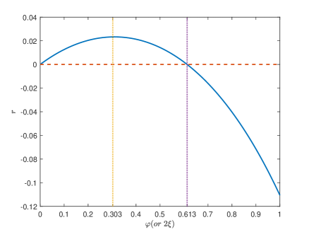
Figure 2: The violation ratio $r$ for the first (second) inequality, as a function of $\varphi$ ($2\xi$ ) for $\eta_{c}$ ($\chi_{c_{0}}$).

3.2 The process with polarization effects

Now we consider the process $e^{+}e^{-}\to\Lambda\bar{\Lambda}\to p\pi^{0}\bar{p}\pi^{+}$ and $e^{+}e^{-}\to J/\Psi\to\Lambda\bar{\Lambda}\to p\pi^{0}\bar{p}\pi^{+}$, with polarizations. The joint angular distribution can be parameterized as LambdaPRL ; LambdaNature

$$\begin{split}&\frac{d\sigma}{d\Omega_{\Lambda}d\Omega_{p}d\Omega_{\bar{p}}}\propto 1+\eta\cos^{2}\theta_{\Lambda}-\alpha^{2}_{\Lambda}\left(\sin^{2}\theta_{\Lambda}\left(n_{px}n_{\bar{p}x}-\eta n_{py}n_{\bar{p}y}\right)+\left(\cos^{2}\theta_{\Lambda}+\eta\right)n_{pz}n_{\bar{p}z}\right)\\ &-\alpha^{2}_{\Lambda}\sqrt{1-\eta^{2}}\cos(\Delta\Phi)\sin\theta_{\Lambda}\cos\theta_{\Lambda}\left(n_{px}n_{\bar{p}z}+n_{pz}n_{\bar{p}x}\right)\\ &+\alpha_{\Lambda}\sqrt{1-\eta^{2}}\sin(\Delta\Phi)\sin\theta_{\Lambda}\cos\theta_{\Lambda}(n_{py}-n_{\bar{p}y}),\\ \end{split}$$ (12)

where $n_{px}$ is the x-component of $n_{p}$, and so on, $\theta_{\Lambda}$ is the angle between momenta of $\Lambda$ and $e^{-}$, as shown in Fig. 1, $\eta$ and $\Delta\Phi$ are parameters related to polarization effects. It has been noticed that, the maximal violation of BI is related to degree of entanglement ViolationOfBI . We find that the violation of BI given in Ref. MomemtumRepresentation reaches the maximum when $\theta_{\Lambda}=\pi/2$, where the polarization effect is minimal. Therefore we consider this region, where incidently the event number is found to be large in experiments LambdaPRL ; LambdaNature . Hence we only consider these events, for which

$$\begin{split}&\frac{d\sigma(\theta_{\Lambda}=\frac{\pi}{2})}{d\Omega_{p}d\Omega_{\bar{p}}}\propto 1-\alpha^{2}_{\Lambda}\left(n_{px}n_{\bar{p}x}-\eta n_{py}n_{\bar{p}y}+\eta n_{pz}n_{\bar{p}z}\right)\\ \end{split}$$ (13)

Therefore we find

$$\begin{split}&\hat{E}^{\bf xy}_{4}(\xi)=-\frac{\alpha^{2}_{\Lambda}}{9}\eta\cos(2\xi),\;\;\hat{E}^{\bf zy}_{4}(\xi)=-\frac{\alpha^{2}_{\Lambda}}{9}\frac{1+\eta}{2}\cos(2\xi).\end{split}$$ (14)

If our second inequality Eq. (9) is violated, the violation is maximal at $\xi=\pi-\tan^{-1}\left(u_{N}/\sqrt{\left(1+3\eta\right)^{2}-u_{N}^{2}}\right)$. For this maximal violation ratio to be positive, the necessary condition is $\eta>\left(1+\sqrt{4-u_{N}^{2}}\right)/3\approx 0.97$, as shown in Fig. 3. However, it is known from the experiments that $\eta=0.46$ for $e^{+}e^{-}\to J/\psi\to\Lambda\bar{\Lambda}$ LambdaNature , and $\eta=0.12$ for $e^{+}e^{-}\to\Lambda\bar{\Lambda}$ LambdaPRL . Therefore this inequality cannot be violated in either case. Besides, for any $\eta$, the first inequality Eq. (6) cannot be violated.

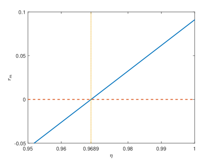
Figure 3: The maximum $r_{m}$ of the violation ratio $r$, as a function of the parameter $\eta$, for entangled $\Lambda\bar{\Lambda}$ pairs with polarization effects.

4 Summary and discussions

In this Letter, we consider local realistic theories with the specifications that the local hidden variables for different objects with spacelike distances are separated and that the physical states are statistical mixtures of subensembles with definite polarizations. We present two inequalities that are shown to be violated by entangled baryons.

In the usual BI test using entangled spins or polarizations, one needs to choose the guide axis of the measurement. When the choices of the two guild axes are not independent, or only limited choices of the axes are allowed, or the guide axes are determined by hidden variables, it is possible that even a local realistic theory can violate BI. This measurement-setting or free-will loophole has been a general defect in most of the previous approaches to BI based on decays of high energy particles. In using $\Lambda\to p\pi^{-}$ ($\bar{\Lambda}\to\bar{p}\pi^{+}$), where the momentum direction of the proton (antiproton) acts as an effective guide axis for the the spin of $\Lambda$ ( $\bar{\Lambda}$), the momentum of the proton (antiproton) cannot be freely set by the experimentalists, and could be determined by hidden variables carried over from the generation of the entangled particle. All these possibilities are different manifestations of measurement or free-will setting loophole.

In the local realistic theories considered here, the dependence of the guide axes, or the momenta of the protons and the antiprotons, on the hidden variables is taken as an assumption in deriving the inequalities. Therefore the violations of these inequalities close the measurement-setting or free-will loophole once and for all.

We find that for $\eta_{c}\to\Lambda\bar{\Lambda}$ and $\chi_{c0}\to\Lambda\bar{\Lambda}$, our inequalities can be violated. For $e^{+}e^{-}\to\Lambda\bar{\Lambda}$ and $e^{+}e^{-}\to J/\Psi\to\Lambda\bar{\Lambda}$, the inequalities are sensitive to the polarization effect, and cannot be violated.

We propose to test our inequalities in experiments. The relative significance of the violation of the first inequality is $r_{m}\approx 0.0233$. Typically, to observe a relative significance at the order of $10^{-2}$, the number of events are required to be at the order of $1/r_{m}^{2}\sim 10^{4}$. For example, the $\eta_{c}$ can be produced from $J/\Psi\to\gamma\eta_{c}$ at BESIII, with the branch ratio ${\rm Br}\left(J/\Psi\to\gamma\left(\eta_{c}\to\Lambda\bar{\Lambda}\to p\pi^{-}\bar{p}\pi^{+}\right)\right)=9.8\pm 2.6\times 10^{-6}$ MomemtumRepresentation . A data sample of $10$ billion $J/\Psi$ events has been collected by BESIII li , updating the $1.31\times 10^{9}$ events used in the previous analysis LambdaNature . $\eta_{c}$ and $\chi_{c}$ processes, with event numbers up to millions and tens of thousands respectively, are also under analyses in BESIII li . It is likely that the violation of our inequalities can be tested using these data.

- (1) D. R. Inglis, Rev. Mod. Phys. 33, 1 (1961); T. B. Day, Phys. Rev. 121, 1204 (1961); H. J. Lipkin, Phys. Rev. 176, 1715 (1968).
- (2) J. Six, Phys. Lett. B 114, 200, (1982); F. Selleri, Lett. Nuovo Cimento 36, 521, (1983); A. Datta and D. Home, Phys. Lett. A119, 3, (1986); A. Afriat and F. Selleri, The Einstein, Podolsky and Rosen Paradox in Atomic, Nuclear and Particle Physics (Plenum Press, New York, 1998); R. A. Bertlmann, W. Grimus, Phys. Rev. D58, 034014, (1998); R. A. Bertlmann, W. Grimus, and B. C. Hiesmayr, Phys. Rev. D60, 114032, (1999); R. A. Bertlmann, W. Grimus, Phys. Rev. D64, 056004, (2001); A. Apostolakis et al. (CPLEAR collaboration), Phys. Lett. B422, 339, (1998); F. Ambrosino et al. (KLOE Collaboration), Phys. Lett. B642, 315, (2006); Y. Shi, Phys. Lett. B 641, 75, (2006); erratum, ibid, 641, 492, (2006); Y. Shi and Y. L. Wu, Eur. Phys. J. C 55, 477 (2008); G. Amelino-Camelia et al., Europhys. J. C68, 619, (2010); A. J. Bevan et al., Eur. Phys. J. C 74, 3026 (2014).
- (3) R. M. Baltrusaitis et al. (MARK-III Collaboration), Phys. Rev. Lett. 56, 2140, (1986); J. Adler et al. (MARK-III Collaboration), Phys. Rev. Lett. 60, 89, (1988).
- (4) I. Dunietz, J. Hauser and J. L. Rosner, Phys. Rev. D35, 2166, (1987); H. J. Lipkin, Phys. Lett. B219, 474-480, (1989); C. D. Buchanan et al., Phys. Rev. D45, 4088, (1992); A. F. Falk and A. A. Petrov, Phys. Rev. Lett. 85, 252, (2000); M. Gronau, Y. Grossman, J. L. Rosner, Phys. Lett. B508, 37-43, (2001), arXiv:hep-ph/0103110; D. Atwood, A. A. Petrov, Phys. Rev. D71, 054032, (2005), arXiv:hep-ph/0207165; Y. Shi, Eur. Phys. J. C 72, 1907 (2012) Z. J. Huang and Y. Shi, Eur. Phys. J. C 72, 1900 (2013); Y. Shi, Eur .Phys. J. C 73, 2506 (2013), arXiv:1306.2676; Z. J. Huang and Y. Shi, Phys. Rev. D 89, 016018 (2014), arXiv:1307.4459; B. Aubert et al. (BABAR Collaboration), Phys. Rev. Lett 99, 171803, (2007), arXiv:hep-ex/0703021; A. Di Domenico (KLOE Collaboration), Found. Phys. 40, 852, (2010); D. Atwood and A. Soni, Phys. Rev. D82, 036003, (2010); B. Aubert, et al. (BABAR Collaboration), Phys. Rev. D79, 072009, (2009), arXiv:0902.1708; M. Ablikim et al. (BESIII Collaboration), Phys. Lett. B734, 227-233, (2014), arXiv:1404.4691; M. Ablikim et al. (BESIII Collaboration), Phys. Lett. B744, 339-346, (2015), arXiv:1501.01378.
- (5) M. C. Bañuls and J. Bernabéu, Phys. Lett. 464, 117, (1999), arXiv:hep-ph/9908353; M. C. Bañuls and J. Bernabéu, Nucl. Phys. B 590, 19, (2000), arXiv:hep-ph/0005323; J. P. Lees et al. (BaBar Collaboration), Phys. Rev. Lett. 109, 211801, (2012), arXiv:1207.5832; J. Bernabu, F. Martinez-Vidal, P. Villanueva-Perez, JHEP, 1208, 064, (2012), arXiv:1203.0171; J. Bernabu, A. Di Domenico, and P. Villanueva-Perez, Nucl. Phys. B868, 102, (2013), arXiv:1208.0773; E. M. Henley, Time Reversal Symmetry, Int. J. Mod. Phys. E 22, 1330010 (2013); J. Bernabu, F. Martinez-Vidal, Rev. Mod. Phys. 87, 165, (2015), arXiv:1410.1742; J. Bernabu, F. J. Botella, M. Nebot, JHEP, 06, 100, (2016), arXiv:1605.03925; Y. Shi and J. Yang, Phys. Rev. D 98, 075019, (2018), arXiv:1612.07628.
- (6) J. S. Bell, Physics 1, 195-200, (1964).
- (7) J. F. Clauser et al., Phys. Rev. Lett. 23, 880 (1969).
- (8) P. H. Eberhard, Nucl. Phys. B398, 155, (1993); A. Di Domenico, Testing Quantum Mechanics in the Neutral Kaon System at a Phi Factory, Nucl. Phys. B450, 293, (1995), hep-ex/0312032; F. Uchiyama, Phys. Lett. A231, 295, (1997); F. Benatti and R. Floreanini, Phys. Rev. D57, R1332, (1998); A. Bramon and M. Nowakowski, Phys. Rev. Lett. 83, 1, (1999); R. A. Bertlmann, W. Grimus, B.C. Hiesmayr, Phys. Lett. A289, 21-26, (2001), arXiv:quant-ph/0107022; N. Gisin and A. Go, Am. J. Phys. 69, 264, (2001); R. H. Dalitz and G. Garbarino, Nucl. Phys. B606, 483 (2001), arXiv:quant-ph/0011108; A. Go (Belle Collaboration), J. Mod. Opt. 51, 991, (2004), arXiv:quant-ph/0310192. J. Li and C. F. Qiao, Phys. Rev. D 74, 076003, (2006).
- (9) N. A. Tönqvist, Found. Phys. 11, 171-177, (1981); N. A. Tönqvist, Phys. Lett. A117, 1, (1986); S. P. Baranov, J. Phys. G: Nucl. Part. Phys. 35, 075002, (2008); X. Hao, H. Ke, Y. Ding, P. Shen and X. Li, Chin. Phys. C34, 311-318, (2010); B. C. Hiesmayr, Sci. Rep. 5, 11591, (2015).
- (10) S. Chen, Y. Nakaguchi and S. Komamiya, Prog. Theor. Exp. Phys. 2013, 063A01 (2013).
- (11) S. A. Abel, M. Dittmar and H. Dreiner, Phys. Lett. B 280, 304-312, (1992); R. A. Bertlmann, A. Bramon, G. Garbarino and B.C. Hiesmayr, Phys. Lett. A332, 355-360, (2004), arXiv:quant-ph/0409051; A. Bramon, R. Escribano and G. Garbarino, J. Mod. Opt. 52, 1681-1684, (2005), arXiv:quant-ph/0410122.
- (12) J. Handsteiner et al., Phys. Rev. Lett. 118, 060401, (2017); M. Li et al., Phys. Rev. Lett. 121, 080404 (2018); The BIG Bell Test Collaboration, Nature 557, 212 (2018).
- (13) Y. Shi, J. Yang, arXiv:1909.10626.
- (14) A. J. Leggett, Found. Phys. 33, 1469, (2003).
- (15) S. Gröblacher, T. Paterek, R. Kaltenbaek, . Brukner, M. Zukowski, M. Aspelmeyer, A. Zeilinger, Nature 446, 871-875, (2007).
- (16) A. Z. Dubnickova, S. Dubnika, and M. P. Rekalo, Nuovo Cimento A109, 241 (1996).
- (17) M. Ablikim et al. (BESIII Collaboration), Phys. Rev. Lett. 123, 122003, (2019).
- (18) M. Ablikim et al. (BESIII Collaboration), Nature Physics. 15, 631-634, (2019).
- (19) M. Ablikim et al. (BESIII Collaboration), Phys. Rev. D91, 112004 (2015), arXiv:1504.02680; D. X. Lin (BESIII Collaboration), Nuclear and Particle Physics Proceedings, 282-284, 111-115, (2017); Alaa Dbeyssi (BESIII Collaboration), EPJ Web of Conferences, 138, 01011, (2017); M. Ablikim et al. (BESIII Collaboration), Phys. Rev. D97, 032013 (2018), arXiv:1709.10236.
- (20) G. Fldt, Eur. Phys. J. A51, 74, (2015); S. Pacetti, R. Baldini Ferroli, and E. Tomasi-Gustafsson, Phys. Rep. 550-551, 1, (2015); V. Punjabi, C.F. Perdrisat, M. K. Jones, E. J. Brash, and C. E. Carlson, Eur. Phys. J. A51, 79, (2015); Gran Fldt, Eur. Phys. J. A52, 141, (2016); J. Haidenbauer, U. G. Meiner, Phys. Lett. B761, 456-461, (2016); Gran Fldt, Andrzej Kupsc, Phys. Lett. B772, 16-20, (2017); Liang-Liang Liu, Chao Wang and Xin-Heng Guo, Chin. Phys. C, 42, 10, (2018), arXiv:1801.08417.
- (21) G. A. Miller, Phys. Rev. Lett. 99, 112001 (2007).
- (22) C. Branciard et al., Phys. Rev. Lett. 99, 210407, (2007), arXiv:0708.0584.
- (23) N. Gisin, Phys. Lett. A 154, 201, (1991).
- (24) H. Li, private communication.