On the Boson-Fermion resonant model on a lattice

Abstract

We review briefly the properties of a mixture of mutually interacting bosons (bound electron pairs) and itinerant fermions on a lattice (the boson-fermion model). The calculations of the superconducting phase transition temperature ($T_{c}$) and the phase diagram are the main concern. The self-consistent $T$-matrix method is applied to determine the superconducting critical temperature from a pseudogap phase. The method takes into account the pairing fluctuations effects. The $T$-matrix results for $T_{c}$ are given for a 3D cubic lattice with tight-binding dispersion of electrons and standard bosons, and they are also compared with those of the BCS- mean-field approximation (MFA). Our results describe the BCS-Bose-Einstein condensation (BEC) crossover in the boson-fermion mixture with resonant interaction. The energy scales involved in the pseudogap formation are also analysed.

1 Introduction

The scenario of coexisting local pairs (LPs) and itinerant electrons (a mixture of charged $2e$ bosons and fermions), i.e. the boson-fermion model, for non-conventional superconductors, chalcogenide glasses, and systems with alternating valence, was introduced about two decades ago [1, 2, 3]. Because of the intersubsystem charge exchange coupling, an induced (resonant) pairing mechanism can be active in this model, which prompts the superconducting state involving both boson and fermion components. A related resonance-boson model of superconductivity was developed in Refs.[4]. A mixture of interacting bosons and itinerant electrons can display superconducting characteristics which are intermediate between those of the local pair superconductors and those of the homogeneous BCS systems [2, 3, 4, 5]. The relevance of this two-component model for high temperature superconductors (HTS) and other short-coherence length superconductors has been the concern of many authors [2, 3, 4, 5, 6, 7, 8, 9, 10, 11, 12, 13, 14, 15, 16, 17, 18, 19, 20, 21, 22, 23]. It has also been applied as the two-channel model for description of the BCS–BEC crossover from the atom Cooper pairs to molecules in ultra-cold fermionic atomic gases with a Feshbach resonance [24, 25, 23].

Even though for HTS the boson-fermion (BF) model has been proposed phenomenologically, it can also be obtained as an effective low-energy model from microscopic formulation. For instance, within the polaron scenario, it has been derived from the generalized periodic Anderson model with on-site hybridization of wide- and narrow-band electrons, in which the narrow-band electrons are locally strongly coupled with the lattice deformation [2]. In this context, LPs (bipolarons) are formed which are hard-core (charged $2e$) bosons made up of two tightly bound fermions. Next, the plaquette BF model, an effective model for hole pairing in cuprates, has been obtained from the strongly correlated Hubbard model on the square lattice by the contractor renormalization method [14]. Several authors have considered the BF scenarios in the investigations of superconductivity mechanism, exploring heterogeneity of the electronic structure of cuprate HTS, especially in the pseudogap phase, either in the momentum space (the Fermi arcs model) [11, 12, 16, 17, 18, 22] or in the real space (charge and spin inhomogeneities) [13, 15].

For a review of two-component scenarios for non-conventional (exotic) superconductors, see Ref. [18]. Also, disorder and inhomogeneity effects have been recently investigated in the (hard core) boson-fermion model for non-conventional superconductors [26, 27].

Thus, the boson-fermion model with resonant interaction is the basic model for superconductivity that has been adopted to explain high-Tc superconductivity and the BCS-BEC crossover in ultra-cold fermionic atomic gases [2, 3, 4, 5, 6, 7, 8, 9, 10, 11, 12, 13, 14, 15, 16, 17, 18, 19, 20, 21, 22, 23, 24, 25, 26, 27, 28, 29, 30, 31, 32, 33].

The purpose of this paper is analysis of the phase diagrams of the BF model on a lattice and detail evaluation of the superconducting transition temperature beyond BCS-MFA. We extend our previous study [19] based on a generalized $T$-matrix approach adapted to the BF model and provide further results. Our method explores the pairing fluctuation theory of the BCS-BEC crossover for single-channel fermion systems with attraction [34, 35, 23, 36, 37]. In Sec.2 we briefly outline the $T$-matrix formalism for the BF model and present derivation of equations which determine $T_{c}$ from the pseudogap phase, not described in Ref.[19]. The numerical solutions to these equations for a simple cubic lattice, with the tight-binding dispersion for fermions, are reviewed in Sec. 3.

2 $T$-matrix formalism: Equations for $T_{c}$ in the Boson–Fermion model

We will consider the boson-fermion model on a lattice described by the following Hamiltonian [19]:

$${\cal{H}}=\sum_{\mathbf{k}\sigma}(\varepsilon_{\mathbf{k}}-\mu)c^{\dagger}_{\mathbf{k}\sigma}c_{\mathbf{k}\sigma}+\sum_{\mathbf{q}}(E^{0}_{\mathbf{q}}+2\Delta_{B}-2\mu)b^{\dagger}_{\mathbf{q}}b_{\mathbf{q}}$$

$$-\frac{U}{N}\sum_{\mathbf{k},\mathbf{k}^{\prime},\mathbf{q}}c^{\dagger}_{\mathbf{k}+\mathbf{q}/2,\uparrow}c^{\dagger}_{-\mathbf{k}+\mathbf{q}/2,\downarrow}c_{-\mathbf{k}^{\prime}+\mathbf{q}/2,\downarrow}c_{\mathbf{k}^{\prime}+\mathbf{q}/2,\uparrow}$$

$$+\frac{I}{\sqrt{N}}\sum_{\mathbf{q}}\left(b^{\dagger}_{\mathbf{q}}B_{\mathbf{q}}+B^{\dagger}_{\mathbf{q}}b_{\mathbf{q}}\right),$$ (1)

$$B^{\dagger}_{\mathbf{q}}=\sum_{\mathbf{k}}c^{\dagger}_{{\mathbf{k}}+{\mathbf{q}}/2,\uparrow}c^{\dagger}_{-{\mathbf{k}}+{\mathbf{q}}/2,\downarrow}~{},$$ (2)

where, $\sigma=\{\uparrow,\downarrow\}$, $c^{\dagger}_{\mathbf{k}\sigma}$ and $c_{\mathbf{k}\sigma}$ are the fermion creation (annihilation) operators with momentum ${\mathbf{k}}$ and spin ${\sigma}$. $b_{\mathbf{q}},b^{\dagger}_{\mathbf{q}}$ represent the boson operators satisfying the standard commutation relations: $[b_{\mathbf{q}},b^{\dagger}_{\mathbf{q}^{\prime}}]=\delta_{{\mathbf{q}}{\mathbf{q}^{\prime}}},[b_{\mathbf{q}},b_{\mathbf{q}^{\prime}}]=0=[b^{\dagger}_{\mathbf{q}},b^{\dagger}_{\mathbf{q}^{\prime}}]$. $B^{\dagger}_{\mathbf{q}}$ stands for the singlet pair creation operator of $c$-electrons. $\varepsilon_{\mathbf{k}}$ is the electron band energy, $E^{0}_{\mathbf{q}}$ is the boson kinetic energy, and they are both defined on the hypercubic lattice. $E^{0}_{\mathbf{0}}=0$. $2\Delta_{B}$ is the bottom of the boson band and $\mu$ is the chemical potential. $I$ is the intersubsystem (resonant) coupling constant. $U$ - the direct (non-resonant) interaction between fermions. The total number of particles per site is $n=n_{F}+2n_{B}$, where $n_{F}=\frac{1}{N}\sum_{\mathbf{k}\sigma}\langle c^{\dagger}_{\mathbf{k}\sigma}c_{\mathbf{k}\sigma}\rangle$ is the electron concentration and $n_{B}=\frac{1}{N}\sum_{\mathbf{q}}\langle b^{\dagger}_{{\mathbf{q}}}b_{\mathbf{q}}\rangle$ - the boson concentration, $N$ - the number of lattice sites.
The inherent property of the model is the presence of pair exchange interaction ($I$) (or interconversion term), i.e. when a boson is created ($b^{\dagger}_{{\mathbf{q}}}$) simultaneously a singlet-pair of c-electrons is annihilated ($B_{\mathbf{q}}$) and vice versa. If $I=0$, we have two subsystems decoupled from each other and they can undergo a transition at $T_{BCS}$ (at weak $U$, for fermions) and $T_{BEC}$ (for bosons). However, if the intersubsystem interaction $I\neq 0$, one common transition to the superfluid state will occur.
At first we consider the case of the absence of the direct fermion interaction, i.e. the case of $U=0$.

In the self-consistent $T$-matrix approximation the fermionic ($G(k)$) and bosonic ($D(q)$) Green’s functions (GF) in the normal state satisfy the equations [5, 7]:

$$G(k)=\frac{1}{G_{0}^{-1}(k)-\Sigma_{F}(k)}~{},$$ (3)

$$\Sigma_{F}(k)=\sum_{q}\Gamma(q)G(q-k)~{},$$ (4)

$$\Gamma(q)=I^{2}D(q)~{},$$ (5)

$$D(q)=\frac{1}{D^{-1}_{0}(q)-\Sigma_{B}(q)}~{},$$ (6)

$$\Sigma_{B}(q)=-I^{2}\Pi(q)~{},$$ (7)

$$\Pi(q)=\sum_{k}G(k)G(q-k)~{},$$ (8)

where we used the four-vector notation: $k=({\mathbf{k}},i\omega_{n}),~{}q=({\mathbf{q}},i\nu_{m})$, $\sum_{k}=\frac{1}{\beta N}\sum_{{\mathbf{k}}}\sum_{\omega_{n}}$, $\sum_{q}=\frac{1}{\beta N}\sum_{{\mathbf{q}}}\sum_{\nu_{m}}$. $\omega_{n}=(2n+1)\pi/\beta$ and $\nu_{m}=2m\pi/\beta$ are the fermionic and bosonic Matsubara frequencies, respectively. $\beta=1/k_{B}T$. The free fermionic GF is $G_{0}^{-1}(k)=i\omega_{n}-{\bar{\varepsilon}_{\mathbf{k}}}$, while the free bosonic GF: $D^{-1}_{0}(q)=i\nu_{m}-2{\bar{\Delta}_{B}}-E^{0}_{\mathbf{q}}$. ${\bar{\varepsilon}}_{\mathbf{k}}=\varepsilon_{\mathbf{k}}-\mu$, $\bar{\Delta}_{B}=\Delta_{B}-\mu$. $\Sigma_{F}(k)$ and $\Sigma_{B}(q)$ are the fermion and boson self-energies, respectively. $\Pi(q)$ is the pair susceptibility and $\Gamma(q)$ - the $T$-matrix.

The basic idea in the calculations of the critical temperature consists in the following approximation for the fermionic self-energy $\Sigma_{F}(k)$. We consider only slow fluctuations of the pairing field and neglect temporal and spatial variations, i.e. the terms with $q\approx 0$ are the dominant ones in Eq.(4) [35, 38, 39]

$$\Sigma_{F}(k)\approx G_{0}(-k)\sum_{q}\Gamma(q)=\frac{\Delta_{pg}^{2}}{i\omega_{n}+{\bar{\varepsilon}_{-{\mathbf{k}}}}}\,.$$ (9)

$$\Delta_{pg}^{2}=-\sum_{q}\Gamma(q)=-\frac{1}{\pi N}\sum_{\mathbf{q}}\int_{-\infty}^{\infty}Im\Gamma({\mathbf{q}},\Omega)b(\Omega)d\Omega\,,$$ (10)

$b(\Omega)=1/\left[\exp{(\beta\Omega)}-1\right]$ is the Bose function. Eq.(10) determines a pseudogap parameter $\Delta_{pg}$. The fermionic GF (Eq.(3)) takes the following form:

$$G(k)=\frac{i\omega_{n}+{\bar{\varepsilon}_{\mathbf{k}}}}{(i\omega_{n})^{2}-E_{\mathbf{k}}^{2}}\;,\;E_{\mathbf{k}}=\ \sqrt{{\bar{\varepsilon}_{\mathbf{k}}}^{2}+\Delta_{pg}^{2}}\,,$$ (11)

which is reminiscent of the standard BCS expression with the quasiparticle energy $E_{\mathbf{k}}$. Using this GF, the pair susceptibility $\Pi(q)$ is calculated. In the following instead of the full calculation of $\Pi(q)$ [38, 39, 37] the partial dressing is adopted which was considered in detail by Kadanoff and Martin [40] and Levin et al. [35]

$$\Pi(q)\approx\sum_{k}G(k)G_{0}(q-k)~{},$$ (12)

which with the use of Eq.(11) and after performing the summation over the Matsubara frequencies takes the form:

$$\Pi(q)=-\frac{1}{N}\sum_{\mathbf{k}}\left[\frac{f(E_{\mathbf{k}})+f({\bar{\varepsilon}_{{\mathbf{q}}-{\mathbf{k}}}})-1}{{\bar{\varepsilon}_{{\mathbf{q}}-{\mathbf{k}}}}+E_{\mathbf{k}}-i\nu_{m}}u_{\mathbf{k}}^{2}+\frac{f({\bar{\varepsilon}_{{\mathbf{q}}-{\mathbf{k}}}})-f(E_{\mathbf{k}})}{{\bar{\varepsilon}_{{\mathbf{q}}-{\mathbf{k}}}}-E_{\mathbf{k}}-i\nu_{m}}v_{\mathbf{k}}^{2}\right]\;,$$ (13)

$u_{\mathbf{k}}^{2}+v_{\mathbf{k}}^{2}=1$,   $u_{\mathbf{k}}^{2}=\frac{1}{2}(1+\frac{{\bar{\varepsilon}_{\mathbf{k}}}}{E_{\mathbf{k}}})$, $f(\omega)=1/\left[\exp{(\beta\omega)}+1\right]$ is the Fermi function.

In the single channel fermion system the $T$-matrix is given by $\Gamma^{-1}(q)=g^{-1}+\Pi(q)$, where $g$ is the coupling constant. Thus, the condition $\Gamma^{-1}(0)=0$ determines $T_{c}$ and we obtain the system of three coupled equations for $\Delta_{pg}$, $T_{c}$ and $\mu$, which were studied in detail for the continuum and lattice fermions with attractive interaction in Refs.[23, 35, 37]. We call this $T$-matrix approach as the $(GG_{0})G_{0}$ scheme, which indicates the way the Greens functions enter the pair susceptibility and the fermion self-energy.

In our boson-fermion model we have to consider the bosonic GF Eq.(6), which is given by

$$\Gamma(q)=I^{2}D(q)=\frac{I^{2}}{i\nu_{m}-2{\bar{\Delta}_{B}}-E^{0}_{\mathbf{q}}+I^{2}\Pi(q)}\,.$$ (14)

The divergence of the generalized $T$-matrix $\Gamma(q)$ at $q=0$, i.e. $({\mathbf{q}}=0,\Omega=0)$ is the same as for the bosonic GF $D(q)$ and yields the equation for $T_{c}$:

$$2{\bar{\Delta}_{B}}+E^{0}_{\mathbf{0}}-I^{2}\Pi(0)=0\;,$$ (15)

$$2{\bar{\Delta}_{B}}+E^{0}_{\mathbf{0}}=\frac{I^{2}}{N}\sum_{\mathbf{k}}\frac{\tanh(\beta_{c}E_{\mathbf{k}}/2)}{2E_{\mathbf{k}}}~{},$$ (16)

where we used Eq.(13): $\Pi(0)=\Pi({\mathbf{0}},0;T_{c})=\frac{1}{N}\sum_{\mathbf{k}}\frac{\tanh(\beta_{c}E_{\mathbf{k}}/2)}{2E_{\mathbf{k}}}~{}.$ The number of fermions is given by:

$$n_{F}=\frac{2}{\beta N}\sum_{{\mathbf{k}},\,\omega_{n}}e^{i\omega_{n}\eta}G(k)=\frac{1}{N}\sum_{\mathbf{k}}\left[1-\frac{{\bar{\varepsilon}_{\mathbf{k}}}}{E_{\mathbf{k}}}\tanh{(\beta_{c}E_{\mathbf{k}}/2)}\right]\;.$$ (17)

The number of bosons is:

$$n_{B}=-\frac{1}{\beta N}\sum_{{\mathbf{q}},\,\nu_{m}}e^{i\nu_{m}\eta}D(q)=-{\frac{1}{\pi N}\sum_{\mathbf{q}}}\int_{-\infty}^{\infty}ImD({\mathbf{q}},\Omega)b(\Omega)d\Omega\;.$$ (18)

($\eta=0^{+}$). The total number of particles in the system $n$ is conserved

$$n=n_{F}+2n_{B}\;.$$ (19)

Thus, by comparing Eq.(10) and Eq.(18) one gets that at $T_{c}$:

$$\Delta_{pg}^{2}=I^{2}n_{B}\;.$$ (20)

The above system of self-consistent equations (10,16,19,20) determines $\Delta_{pg}$, $T_{c}$ and the chemical potential $\mu$. In comparison with BCS-MFA, we have taken into account the boson self-energy effect and included pairing fluctuations.

Next, we examine the direct interaction between fermions. The effect of $U$ will be included in the Random Phase Approximation - like method, just treating it in the ladder approximation [8, 25]. This amounts to generalization of the $T$-matrix as follows:

$$\Gamma(q)=\frac{-U_{eff}(q)}{1-U_{eff}(q)\Pi(q)}~{},$$ (21)

where $U_{eff}(q)=U-I^{2}D_{0}(q)$ is the effective pairing interaction and the bosonic self-energy is given by:

$$\Sigma_{B}(q)=-I^{2}{\tilde{\Pi}}(q)~{},~{}{\tilde{\Pi}}(q)=\frac{\Pi(q)}{1-U\Pi(q)}~{}.$$ (22)

The transition temperature is given by the Thouless criterion of the divergent $T$-matrix, i.e. $1-U_{eff}(0)\Pi(0)=0$. Simultaneously one checks that the bosonic GF is divergent indicating a common transition in the system. The pseudogap parameter and the number of bosons still satisfy the same general equations (10) and (18).

Furthermore, in the numerical calculations of $T_{c}$, we use the following procedure to determine the pseudogap parameter $\Delta_{pg}$. Such a procedure should be reasonable for moderate to strong intersubsystem coupling. The analytically continued pair susceptibility (Eq.(13)) has the expansion:

$$\Pi({\mathbf{q}},\Omega)-\Pi(0,0)\approx A_{0}^{\prime}(\Omega-\Omega_{{\mathbf{q}}})+iA_{0}^{\prime\prime}\Omega\;.$$ (23)

We make an assumption that: $\epsilon\equiv A_{0}^{\prime\prime}/A_{0}^{\prime}\ll 1$ , and use te relation: $\lim_{\epsilon\rightarrow 0}\frac{\epsilon}{x^{2}+\epsilon^{2}}=\pi\delta(x)$. Using Eq.(10) and Eq.(15), the equation for pseudogap parameter takes the following form at $T_{c}$ for $U=0$:

$$\Delta_{pg}^{2}=\frac{I^{2}}{1+I^{2}A_{0}^{\prime}}{\frac{1}{N}}\sum_{\mathbf{q}\neq 0}b\left(\frac{E^{0}_{\mathbf{q}}+I^{2}A_{0}^{\prime}\Omega_{\mathbf{q}}}{1+I^{2}A_{0}^{\prime}}\right)~{},$$ (24)

$$\Omega_{\mathbf{q}}=\frac{1}{A_{0}^{\prime}}\frac{1}{N}\sum_{\mathbf{k}}\left[\frac{f(E_{\mathbf{k}})+f({\bar{\varepsilon}}_{{\mathbf{q}}-{\mathbf{k}}})-1}{{\bar{\varepsilon}}_{{\mathbf{q}}-{\mathbf{k}}}+E_{\mathbf{k}}}u_{\mathbf{k}}^{2}+\frac{f({\bar{\varepsilon}}_{{\mathbf{q}}-{\mathbf{k}}})-f(E_{\mathbf{k}})}{{\bar{\varepsilon}}_{{\mathbf{q}}-{\mathbf{k}}}-E_{\mathbf{k}}}v_{\mathbf{k}}^{2}\right.$$

$$+\left.\frac{1-2f(E_{\mathbf{k}})}{2E_{\mathbf{k}}}\right]\;,\;\;$$ (25)

$$A_{0}^{\prime}=\frac{1}{2\Delta_{pg}^{2}}\left[n_{F}-\frac{1}{N}\sum_{\mathbf{k}}2f(\bar{\varepsilon}_{\mathbf{k}})\right]~{}.$$ (26)

We point out that two kinds of (coupled) bosonic contributions are present in $\Delta_{pg}$ (Eq.(24)). The one ($\Omega_{\mathbf{q}}$) is from long-lived pairs of $c$-electrons with finite ${\mathbf{q}}$ and the second is from the direct hopping of bosons $E_{\mathbf{q}}^{0}$. The pair dispersion $\Omega_{{\mathbf{q}}}$ in the small ${\mathbf{q}}$ expansion is of the form:

$$\Omega_{{\mathbf{q}}}=C{\mathbf{q}}^{2}=\frac{{\mathbf{q}}^{2}}{2M^{\star}}~{},$$ (27)

$M^{\star}$ is the effective mass.

For the case $I\neq 0$, $U\neq 0$ we obtain the following equation for $T_{c}$:

$$1=\left(U+\frac{I^{2}}{2(\Delta_{B}-\mu)}\right)\frac{1}{N}\sum_{\mathbf{k}}\frac{\tanh(\beta_{c}E_{\mathbf{k}}/2)}{2E_{\mathbf{k}}}~{}.$$ (28)

With the expansion Eq.(23) the pseudogap parameter and the number of bosons satisfy the following equations:

$$\Delta_{pg}^{2}=\frac{I_{eff}^{2}}{1+I_{eff}^{2}A_{0}^{\prime}}{\frac{1}{N}}\sum_{\mathbf{q}\neq 0}b\left(\frac{E^{0}_{\mathbf{q}}+I_{eff}^{2}A_{0}^{\prime}\Omega_{\mathbf{q}}}{1+I_{eff}^{2}A_{0}^{\prime}}\right)~{}~{},$$ (29)

$$I_{eff}^{2}=(2{\bar{\Delta}_{B}}U+I^{2})^{2}/I^{2}~{}~{},$$

$$n_{B}=\frac{1}{1+K_{eff}^{2}A_{0}^{\prime}}{\frac{1}{N}}\sum_{\mathbf{q}\neq 0}b\left(\frac{E^{0}_{\mathbf{q}}+K_{eff}^{2}A_{0}^{\prime}\Omega_{\mathbf{q}}}{1+K_{eff}^{2}A_{0}^{\prime}}\right)~{}~{},$$ (30)

$$K_{eff}^{2}=I^{2}/(1-U\Pi(0))^{2}~{},$$

where $\Omega_{\mathbf{q}}$ and $A_{0}^{\prime}$ are given by Eqs.(2-26) and $\Pi(0)$ by

$$\Pi(0)=\frac{1}{N}\sum_{\mathbf{k}}\frac{\tanh(\beta_{c}E_{\mathbf{k}}/2)}{2E_{\mathbf{k}}}.$$ (31)

Using Eq.(28) and expression for $I_{eff}^{2}$ one gets $K_{eff}^{2}=I_{eff}^{2}$, thus a similar relationship to that of (20) holds at $T_{c}$:

$$\Delta_{pg}^{2}=I_{eff}^{2}n_{B}~{}.$$ (32)

The above equations for $T_{c}$ and $\Delta_{pg}$ have to be solved together with the condition for conservation of the total number of particles (19), where $n_{F}$ is given by Eq.(17). [19].

3 Numerical results

The numerical solutions to the equations for $T_{c}$ are presented below for a simple cubic (sc) lattice. The electron band energy is given by: $\varepsilon_{\mathbf{k}}=D(1-\gamma_{\mathbf{k}})$; $D=zt$, $\gamma_{\mathbf{k}}=\left[\cos(k_{x})+\cos(k_{y})+\cos(k_{z})\right]/3$, where $t$ - nearest neighbour hopping parameter of c-electrons and $z$ -the coordination number. For the kinetic energy of free bosons we take: $E^{0}_{\mathbf{q}}=J_{0}-J_{{\mathbf{q}}}$ $J_{\mathbf{q}}=J_{0}\gamma_{\mathbf{q}},~{}J_{0}={\it z}J$, $J$ -the direct boson hopping amplitude. The momentum summations are over the first Brillouin zone. Furthermore, in the plots we will use the half of the electron bandwidth ($D$) as an energy unit.

Figs.1-3 show the plots of $T_{c}$, $\Delta_{pg}(T_{c})$, and $\mu(T_{c})$, together with fractions of $n_{F}$ and $n_{B}$ versus the bosonic level position $\Delta_{B}$, across the BCS-BEC crossover. (See also Fig.1 in Ref. [19], for different $n$ and interaction parameters). The direct boson hopping (Figs.1,3) and interaction between fermions are taken into regard (Figs.1-3). In Figs. (1,3) we set $E^{0}_{\mathbf{q}}\simeq J{\mathbf{q}}^{2}$ and $J/t=1/2$ , this corresponds to $m_{B}=2m_{F}$, where $m_{B}=1/(2J)$, $m_{F}=1/(2t)$ are (bare) masses of bosons and fermions on the lattice, respectively, ($\hbar=a=1$, $a$ - the lattice spacing).

As it is clearly seen from Fig.1 and 2 the superfluid phase transition changes in a smooth way from BCS-like to BEC-like when the pairing correlations are incorporated.

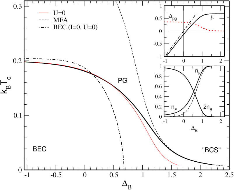
Figure 1: Computed self-consistent $T$-matrix results for the boson-fermion model with resonant interaction (units $D=1$). $n=0.45$, $|I_{0}|/D=0.75$, ($I=-|I_{0}|$), $U/D=0.125$, $D=6t$. $J/t=0.5$. The superfluid transition temperature obtained in $T$-matrix: $T_{c}$ vs $\Delta_{B}$ is shown by the solid curve; the thin red solid curve is for $U=0$. The dashed curve – the BCS-MFA transition temperature. The dash-dotted curve – the $T_{BEC}$ for free boson-fermion mixture but with the constraint $n=n_{F}+2n_{B}$. Upper inset shows the variation of chemical potential $\mu(T_{c})$ (solid curve) and pseudogap parameter $\Delta_{pg}(T_{c})$ (red dotted curve) vs $\Delta_{B}$ ; the dash-dotted line – the chemical potential for BEC transition without interactions ($\mu=\Delta_{B}$). Lower inset: fractions of $n_{F}$, $n_{B}$ and $n^{0}_{F}$ (dashed) vs $\Delta_{B}$ at $T_{c}$, normalized to the total n, across the BCS-BEC crossover; $n^{0}_{F}$-fraction of unpaired fermions at $T_{c}$. See also Fig.1 in Ref.[19].

Let us summarize the main features of three regimes of this evolution.
(i) The renormalized level energy (by the boson self-energy) $\Delta^{*}_{B}$ is negative, i.e. $2\Delta^{*}_{B}=2\Delta_{B}+\Sigma_{B}(q)<0$. In such boson predominant region, the bosons are essentially undamped (do not decay), the $\mu$ is negative, and for large negative $\Delta_{B}$, the $T_{c}$ approaches the $T_{BEC}$ for free bosons from below. What is more, the strong effective attractive interaction mediated by the bosons leads to formation of preformed fermion pairs on the bosonic side of the crossover (compare $n_{F}$ and $n^{0}_{F}$ in lower inset in Fig.1).
(ii) If $\Delta^{*}_{B}>0$, the interconversion boson-pair of fermions (c-electrons) process gives rise to the resonance superfluidity and to the elevation of $T_{c}$. In addition, the range of resonant (or mixed) superfluidity is associated with a pseudogap (PG).
(iii) At last, in the BCS-like regime, predominant by fermions, the boson fraction $n_{B}/n$ is small, and $T_{c}$ approaches the BCS-MFA result. In this case the chemical potential is very close to the Fermi energy and the pseudogap becomes quite small (upper and lower inset in Fig.1). Even a weak direct attraction $U$ enlarges the BCS-like regime (See Fig.1 for $U/D=0.125$ and $U=0$, respectively), but the repulsive $U$ reduces it [19].

It is clear that with decreasing $J$, the BEC asymptote to $T_{c}$ will be lower because of larger $m_{B}$, however the BCS-like regime will be only little affected because of small $n_{B}$. In consequence, the smooth crossover plot of $T_{c}$ will exhibit a round maximum inside the resonance regime for a definite $J/t<0.5$.

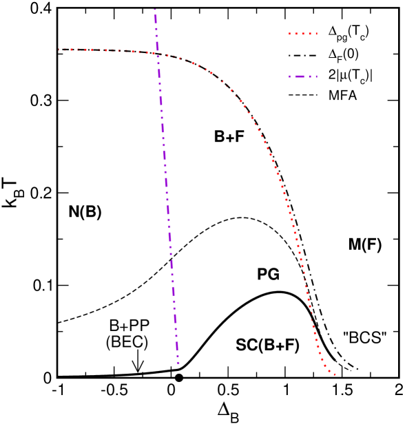
Figure 2: Phase diagram of the boson-fermion model on a sc lattice with the direct boson hopping suppressed (units $D=1$). $n=1$, $|I_{0}|/D=0.5$, $U/D=0.05$, $J=0$. The solid line shows $T_{c}$ vs. $\Delta_{B}$ calculated from the self-consistent $T$-matrix approach. The dash-double-dotted line is for the chemical potential (from $T$-matrix) when $\mu$ is negative. B+PP - region of hybridized bosons and preformed pairs of c-electrons. SC(B+F) - resonance superconductivity phase. M(F) - metallic phase dominated by fermions. PG - pseudogap region. N(B) - normal phase dominated by bosons. Dot marks the crossover point in the superconducting ground state. See text.

Fig.2 shows the phase diagram of the BF model in the case when the direct boson hopping is suppressed ($J=0$), i.e. the bosons are initially immobile, and $n=n_{F}+2n_{B}=1$. It has been obtained from $T$-matrix calculations supplemented by the analysis of superconducting ground state in BCS-MFA [7]. Let us stress that the presence of the resonant coupling ($I$) alone is sufficient to establish superfluidity in the BF mixture, with the region of resonance (or mixed) superfluid. In addition (Fig.2), the energy scale for the pseudogap obtained in the $T$-matrix ($\Delta_{pg}(T_{c})$) is compared with the superconducting gap parameter at $T=0K$ ($\Delta_{F}(0)$), determined in the BCS-MFA. We note that these characteristic parameters are close to each other in the regime dominated by bosons and differ in the BCS-like regime. The MFA $T_{c}$ (thin dashed line in Fig.2), beyond the BCS-region, provides only the pairing scale for the formation of incoherent Cooper (fermion) pairs, and bounds a PG region. The dash-double-dotted line for $2\mu$ negative (being close to the molecule binding energy) separates the bosonic regime. In the bosonic regime (B+PP) we have hybridized bosons and preformed fermion pairs, with the unique branch of excitations given by the pole of bosonic GF $D(\mathbf{q},\Omega)$.

In our numerical computations we assumed the parabolic spectrum for the bosons, but keep the full tight-binding dispersion for the fermions. It was mainly dictated by the simplifications due to the long-wave expansion of the pair susceptibility. For the parabolic boson dispersion we have a simple result for BEC transition of free bosons $k_{B}T_{c}/2J=\frac{2\pi}{\zeta(3/2)^{2/3}}n_{B}^{2/3}=3.3125n_{B}^{2/3}$. Inclusion of the lattice dispersion for bosons $E^{0}_{\mathbf{q}}$, is numerically possible, and it results in quantitative improvement of $T_{c}$, in the BEC regime [7].

3.1 Low-density and broad resonance case

In this subsection we discuss the low density case. For moderate resonant coupling $I$ the evolution of $T_{c}$ vs $\Delta_{B}$ is similar to that presented above. Particularly interesting case is the limit of large $I$, large $\Delta_{B}$, for low density (in cold gases referred to as a broad resonance). We observe that in such a case ($I\rightarrow\infty,\Delta_{B}\rightarrow\infty$, but $-\frac{I^{2}}{2\Delta_{B}}$ finite) the model effectively reduces to the single band (or one-channel) fermion model with an effective attraction. Fig.3 shows the numerical results for (relatively) large coupling $I$. In contrast to the continuum model, with decreasing $\Delta_{B}$ the critical temperature sharply decreases away from the unitarity (before reaching $T_{BEC}$), which is specific to the lattice model. In Fig.3, in the fermion dominated regime, we find that $T_{c}$ in the BF model determined in the $T$-matrix approach, practically follows the behavior of $T_{c}$ in the attractive Hubbard model with an effective attraction ${\bar{U}}_{eff}=U+\frac{I^{2}}{2\Delta_{B}}$.

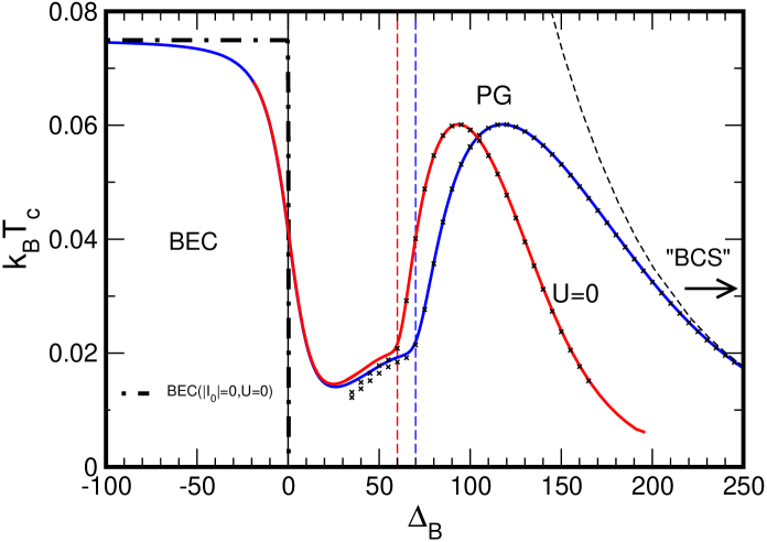
Figure 3: Evolution of $T_{c}$ from BEC to BCS like limit calculated in the $T$-matrix approach for large intersubsystem coupling and low density (units $D=1$). $n=0.1$, $|I_{0}|/6t=15$, $U/6t=0.25$, $J/t=0.5$ $~{}(m_{B}=2m_{F})$. The denotations as in Fig.1. Crosses mark $T_{c}$ obtained in $T$-matrix for the Hubbard model with an effective attraction ${\bar{U}}_{eff}$ and filling $n_{F}=0.1$. The dashed curve is for BCS-MFA. Thin dashed vertical lines denote the points for which the chemical potential passes zero, thus marking the beginning of a Bose regime.

4 Outlook

In summary, we have further investigated the superfluid phase transition temperature and the phase diagram of the boson-fermion model with resonant interaction on the lattice. We also discussed, in terms of $T$-matrix many-body formalism, the way the pseudogap physics can be incorporated in the description of boson-fermion system with resonant interaction. The results obtained, describe mostly the BCS-BEC crossover for $T_{c}$, with variable bosonic (LP) level position, and complement those of Ref.[19]. The interesting region of the resonant (or mixed) superconductivity is preceded by the pseudogap appearing because of pairing fluctuations.

We considered the BF system with standard lattice bosons, however the presented approach can be extended to the important case of hard-core bosons [18, 7, 19]. In addition, our study can be applied to: (i) the BF model with resonant d-wave pairing on quasi 2D lattice [7] (ii) description of the BCS-BEC crossover in a neighbourhood of the quantum superfluid-band insulator transition, which occurs in the model (2) for n=2 [2, 7],[32]. Another extension concerns the application of the $(GG)G_{0}$ $T$-matrix scheme to the BF model [7, 37].

The boson-fermion model we studied can also be treated as special case of a general coupled boson-fermion-Hubbard model written in the Wannier basis:

$${\cal H}={\cal H}_{B}+{\cal H}_{F}+{\cal H}_{1},$$ (33)

$${\cal H}_{B}=\sum_{i}(2\Delta_{B}-2\mu)b^{\dagger}_{i}b_{i}-\sum_{i,j}J_{ij}b^{\dagger}_{i}b_{j}+\frac{1}{2}U_{B}\sum_{i}n^{B}_{i}(n^{B}_{i}-1),\$$ (34)

$${\cal H}_{F}=\sum_{i,j,\sigma}t_{ij}c^{\dagger}_{i\sigma}c_{j\sigma}+\sum_{i,\sigma}(D-\mu)c^{\dagger}_{i\sigma}c_{i\sigma}+\frac{1}{2}U_{F}\sum_{i}n^{F}_{i}(n^{F}_{i}-1),$$ (35)

$${\cal H}_{1}=I\sum_{i}(b^{\dagger}_{i}c_{i\downarrow}c_{i\uparrow}+c^{\dagger}_{i\uparrow}c^{\dagger}_{i\downarrow}b_{i})+U_{BF}\sum_{i}n^{F}_{i}n^{B}_{i},$$ (36)

and $n=n_{F}+2n_{B}.$
$n^{F}_{i}=n_{i\uparrow}+n_{i\downarrow}$, $n_{i\sigma}=c^{\dagger}_{i\sigma}c_{i\sigma}$, $n^{B}_{i}=b^{\dagger}_{i}b_{i}$. $[b_{i},b^{\dagger}_{j}]=\delta_{ij}$. $\{c_{i\sigma},c^{\dagger}_{j\sigma^{\prime}}\}=\delta_{ij}\delta_{\sigma\sigma^{\prime}}$ $n_{F}=\frac{1}{N}\sum_{i\sigma}\langle n_{i\sigma}\rangle$, $n_{B}=\frac{1}{N}\sum_{i}\langle n^{B}_{i}\rangle$. $D=zt$. The bosonic part ${\cal{H}}_{B}$ (34) is described by the boson Hubbard model with the on-site repulsion $U_{B}$ and fermionic part ${\cal{H}}_{F}$ (35) by the Hubbard model with the on-site interaction $U_{F}$. The intersubsystem interactions are specified by the interconversion term ($I$) and the boson-fermion repulsion ($U_{BF}$).
If $U_{B}=U_{BF}=0$, after transforming to ${\bf k}$ - space: $c_{j\sigma}=\frac{1}{\sqrt{N}}\sum_{\mathbf{k}}e^{i{\mathbf{k}}\cdot{\mathbf{R}}_{j}}c_{\mathbf{k}\sigma},~{}b_{j}=\frac{1}{\sqrt{N}}\sum_{\mathbf{q}}e^{i{\mathbf{q}}\cdot{\mathbf{R}}_{j}}b_{\mathbf{q}}$, we obtain the boson-fermion model (2), where $\varepsilon_{\mathbf{k}}$ ($J_{\mathbf{q}})$ is related to Fourier transform of $t_{ij}$ ($J_{ij}$), $\Delta_{B}\rightarrow\Delta_{B}-J_{0}/2$ and $U_{F}=-U$.
If $U_{B}\rightarrow\infty$, and keeping only the two lowest boson states, one gets the case of hard-core bosons (or pseudospins), which satisfy the Pauli spin $1/2$ commutation relations (see Refs.[2, 19]).
The above general model is of interest for non-conventional superconductors as well as for boson-fermion mixtures loaded in optical lattices.

5 Acknowledgements

I would like to thank S. Robaszkiewicz for helpful discussions.

References

• [1] J. Ranninger and S. Robaszkiewicz, Physica B 135 (1985) p.468; R. Micnas, J.Ranninger, and S. Robaszkiewicz, J. Magn. Magn. Mater. 63-64 (1987) p.420.
• [2] S. Robaszkiewicz, R. Micnas, and J. Ranninger, Phys. Rev. B 36 (1987) p.180.
• [3] R. Micnas, J. Ranninger, and S. Robaszkiewicz, Rev. Mod. Phys. 62 (1990) p.113 and Refs. therein.
• [4] R. Friedberg and T. D. Lee, Phys. Rev. B 40 (1989) p.6745; R. Friedberg, T.D. Lee, and H.C. Ren, Phys. Rev. B 42 (1990) p.4122.
• [5] J. Ranninger and J.M. Robin Sol. State Comm. 98 (1996) p.559; Phys. Rev. B 53 (1996) p.R11961; Phys. Rev. B 56 (1997) p.8330.
• [6] R. Micnas and S. Robaszkiewicz, in ”High-$T{c}$ Superconductivity 1996: Ten Years after the Discovery”, NATO ASI Series E 343 (1997), pp.31-93. (Kluwer, The Netherlands).
• [7] R. Micnas (unpublished).
• [8] T. Kostyrko, Acta Phys. Polon. A91 (1997) p.399.
• [9] T. Domanski and J. Ranninger, Phys. Rev. B 63 (2001) p.134505; ibid. 70 (2004) p.184503.
• [10] J. Ranninger and L. Tripodi, Phys. Rev. B 67 (2003) p.174521.
• [11] V.B. Geshkenbein, L.B. Ioffe, and A.I. Larkin, Phys. Rev. B 55 (1997) p.3173.
• [12] A. Perali, C. Castellani, C. Di Castro, M. Grilli, E. Piegari, and A. A. Varlamov, Phys. Rev. B 62 (2000) p.R9295.
• [13] A.H. Castro Neto, Phys. Rev. B 64 (2001) p. 104509.
• [14] E. Altman and A. Auerbach, Phys. Rev. B 65 (2002) p.104508.
• [15] W.-F. Tsai and S.A. Kivelson Phys. Rev. B 73 (2006) p.214510.
• [16] R. Micnas, S. Robaszkiewicz, and A. Bussmann-Holder, Phys. Rev. B 66 (2002) p.104516.
• [17] R. Micnas, S. Robaszkiewicz, and A.Bussmann-Holder, Physica C 387, 58 (2003).
• [18] R. Micnas, S. Robaszkiewicz, and A. Bussmann-Holder, Structure and Bonding: ”Superconductivity in Complex Systems” 114 (2005), pp.13-69 and Refs. therein.
• [19] R. Micnas, Phys. Rev. B 76 (2007) p.184507.
• [20] A. Mihlin and A. Auerbach, Phys. Rev. 80 (2009) p.134521.
• [21] J. Ranninger and T. Domański, Phys. Rev. B 81 (2010) p.014514.
• [22] Kai-Yu Yang, E. Kozik, Xin Wang, and M. Troyer, Phys. Rev. B 83 (2011) p.214516.
• [23] Q. Chen, J. Stajic, S. Tan, and K. Levin, Phys. Rep. 412 (2005) p.1.
• [24] M. Holland, S. J. J. M. F. Kokkelmans, M. L. Chiofalo, and R. Walser, Phys. Rev. Lett. 87 (2001) p.120406.
• [25] Y. Ohashi and A. Griffin, Phys. Rev. Lett. 89 (2002) p.130402; Phys. Rev. A 67 (2003) p.033603.
• [26] G. Pawłowski, R. Micnas, and S. Robaszkiewicz, Phys. Rev. B 81 (2010) p.064514.
• [27] J. Krzyszczak, T. Domański, K. I. Wysokiński, R. Micnas, and S. Robaszkiewicz, J. Phys: Condens. Matter 22,(2010) p.255702.
• [28] T. Mamedov and M. de Llano, J. Phys. Soc. Jpn. 80(2011) p.074718.
• [29] M. Zapalska and T. Domański, Phys. Rev. B 84 (2011) p.174520.
• [30] Y. Yildirim and W. Ku, Phys. Rev. X 1 (2011) p.011011.
• [31] Chih-Chun Chien, Yan He, Qijin Chen, and K. Levin, Phys. Rev. A77 (2008) p.011601.
• [32] Zhaochuan Shen, L. Radzihovsky, and V. Gurarie, Phys. Rev. Lett. 109 (2012) p.245302;
M. Cuoco and J. Ranninger, Phys. Rev. B 70 (2004) p.104509; ibid. B 74 (2006) p. 094511.
• [33] M. L. Wall and L. D. Car, Phys. Rev. A 87 (2013) p.033601.
• [34] R. Micnas, M. H. Pedersen, S. Schafroth, T. Schneider, J. J. Rodríguez-Núñez, and H. Beck, Phys. Rev. B 52 (1995) p.16223.
• [35] Q. Chen, I.Kosztin, B. Janko, and K. Levin, Phys. Rev. B 59 (1999) p.7083; I. Kosztin, Q. Chen, Y.-J. Kao, and K. Levin, Phys. Rev. B 61 (2000) p.11662.
• [36] R. Micnas, Acta Phys. Polon. 100 (s) (2001) p.177.
• [37] A. Cichy and R. Micnas, Annals of Physics 347 (2014) p.207.
• [38] A. Schmid, Z. Physik 231 (1970) p.324.
• [39] O. Tchernyshyov, Phys. Rev. B 56 (1997) p.3372.
• [40] L. P. Kadanoff and P. C. Martin, Phys. Rev. 124 (1961) p.670.