Full exact solution of the out-of-equilibrium
boundary sine Gordon model

Abstract

The massless boundary sine-Gordon (SG) model is the only interacting impurity model with a known exact solution out-of-equilibrium, yet existing so far only for integer values of the sine Gordon coupling $\lambda$ [Phys. Rev. Lett. 74, 3005 (1995)]. We present here a full exact solution for arbitrary rational values of $\lambda$, at arbitrary voltage $V$ and temperature $T$. We use the “string” solutions of the bulk SG model, here regarded as genuine quasiparticles avoiding charge diffusion in momentum space. We carefully present the finite voltage and temperature thermodynamics of this gas of interacting exotic quasiparticles, whose very nature depends on subtle arithmetic properties of the rational SG parameter $\lambda$, and explicitly check that the string representation is thermodynamically complete. By considering a Loschmidt echo, we derive the exact transmission probability of strings on the impurity. We obtain the exact universal scaling function for the electrical current $I(V,T)$. Our results are in excellent agreement with recent experimental out-of-equilibrium data and question the reality of these exotic quasiparticles.

I Introduction

Large assemblies of interacting entities can be the siege of emergence, i.e. manifestation of more complex “entities” with new features that were absent at the elementary level. Restricting this vastly fertile concept of emergence to the study of its manifestations when elementary entities are the microscopic degrees of freedom of inert matter (electrons, atoms…) is certainly at the heart of condensed matter physics, as expressed by the famous statement by P.W. Anderson: “More is different”MoreIsDifferent . In condensed matter a typical scale for “more” is the number of involved particles $N={\cal O}({{\cal N}_{A}^{\vphantom{\dagger}}})$ with ${{\cal N}_{A}^{\vphantom{\dagger}}}\simeq 6\times 10^{23}$ the Avogadro number, or, best conveying the idea of the complexity in a quantum interacting system, the number of states given by the dimension of the many-body Hilbert space $\mathscr{H}$: $\ln(\mbox{dim}\mathscr{H})={\cal O}({{\cal N}_{A}^{\vphantom{\dagger}}})$. Understanding such correlated systems defines notoriously-hard-to-solve “quantum many-body problem” (QMBP). The other side of the coin of the QMBP is the vast phenomenology of the possible collective arrangement of the microscopic degrees of freedom, leading to the large collection of observed, as well as yet-to-be-discovered, states of matter.

The new, emergent properties of such states of matter can be ultimately traced back to the very nature of the low energy states of the system, which, very often, can be described as collections of “quasiparticles” (QPs) emerging, as the result of interactions, as genuinely new elementary excitations, possessing new features like new quantum numbersWoelfle08 .

Historically the earliest occurence of QPs in the QMBP stems from the study of ${}^{3}\mbox{He}$, a strongly interacting liquid of fermions. The theory that has been developed to describe this situation, the Landau-Fermi liquid theoryFermiLiquids , is also the paradigm for the description of ordinary metals: even in the case where electron-electron interactions are strong, low energy states in a metal are described in terms of emergent QPs, the quasi-electrons, that are (weakly) interacting objects still carrying charge $e$ but with renormalized mass $m^{*}$. Due to certain interactions however, this metal can turn into a BCS superconductorBCS : there the Fermi-liquid picture breaks down, but the concept of QP is still relevant: the groundstate can be described as a condensate of charge $e^{*}=2e$ Cooper pairs, and the QPs describing excitations above it have no definite chargeBookFetterWalecka .

Interactions can shape in an even more dramatic way the nature of QPs: a striking example is provided by Tomonaga-Lüttinger liquids (TLL), that replace the paradigm of Landau-Fermi liquid for massless electrons in one dimension with short-range interactionsLuttinger63 ; BookGiamarchi : there, the notion of quasi-electron becomes ineffectual, QPs exhibit spin-charge separation Auslaender02 ; Jompol09 , and carry fractional charge – in clean realization of chiral TLL in edge states of the $\nu=\frac{1}{3}$ Fractional Quantum Hall state, charge $e^{*}=\frac{e}{3}$ QPs could be observed by noise measurement in the tunnelling current Saminadayar1997 ; dePicciotto1997 . This example emphasizes that tunnelling experiments constitute a central tool to probe the nature of the QPs.

On the theoretical side it is important to keep in mind that the relationship between the original microscopic entities and the emergent QPs is of many-body nature: due to interactions it consists in a change of basis in $\mathscr{H}$ (roughly speaking, a $e^{{\cal N}_{A}^{\vphantom{\dagger}}}\times e^{{\cal N}_{A}^{\vphantom{\dagger}}}$ unitary matrix), making it extremely complex and most of the time out of reach of any exact description. On top of this, a second major difficulty in the theoretical approach stems from the fact that spectroscopic experiments probing the QPs are typically carried on in non-equilibrium situations, whereas the available analytical tools for tackling strong correlations are designed for equilibrium situations. While on the one hand we still clearly lack a general efficient theoretical framework for treating in a controlled way both strong interactions and out-of-equilibrium physics, on the other hand such conditions are routinely produced, controlled and measured with high precision in milli-Kelvin experiments, making any progress in the theoretical effort a valuable one.

With respect to the first difficulty, integrable systems constitute a remarkable exception: they are interacting many-body systems where a rich underlying structure (they enjoy an infinite number of conservation laws) allows for an exact description of the emergent QPs, in spite of strong interactions – see e.g. the spin-charge separation phenomenon in the 1D Hubbard modelBookEsslerHubbard . As ideal 1D systems with no dissipation mechanism, although integrable models can sometimes apply to the description of realistic experimental situations, they cannot address the non-equilibrium regime where dissipation is at play – they can be viewed as sophisticated interacting generalizations of the ideal perfect gas in 1D. The situation at hand is however different for quantum impurity integrable systems, describing homogeneous, free systems, except at one point in space where interaction is concentrated. Since dissipation in a realistic system typically occurs far from the impurity, they can be directly relevant to the quantitive description of coherent transport. Therefore, QIIS are unique systems where one can hope to capture exactly the physics of strong correlations in a non-equilibrium context.

Considerable efforts have been devoted to the description of quantum impurities in out-of-equilibrium situations by numerical approaches implementing elaborate approximate solutions of the QMBP – by using e.g. functional renormalization group (RG) FRG-Review ; Meden08 , real-time RG andergassen10 , time dependent density matrix RG or time dependent numerical RG Schmitteckert14 or fermionic representation for transport through TLL Aristov14 . Yet, numerical approaches ultimately rely on some sort of approximation to tackle the QMBP. Moreover, those methods are usually designed to compute specific physical quantities, so that the access to the nature of the QPs – which we believe is part of the elucidation of the physics – either requires their a priori knowledge or remains out of reach.

The boundary sine Gordon (BSG) model is an archetypical QIIS which, in several respects, plays a central role. First, it has a wide range of applications in condensed matter physics, and even beyond. This variety of realizations has its root in the minimal character of this model, which can be considered as the simplest non-linear impurity model: it describes a free boson $\phi(x)$ interacting via a cosine potential $\cos(\beta\phi(x\!\!=\!\!0))$. Introducing the SG parameter:

$$\lambda\equiv\frac{8\pi}{\beta^{2}}-1$$ (1)

the BSG describes, for example: $(i)$ transport through an impurity in a 1D conducting wire with Tomonaga-Lüttinger parameter $K=\frac{1}{\lambda+1}$KaneFisher92 ; $(ii)$ electron tunnelling between edge states of the Fractional Quantum Hall Effect (FQHE) at filling $\nu=\frac{1}{\lambda+1}$ with $\nu^{-1}$ an integer FLS-PRL ; FLS-PRB ; $(iii)$ low-energy transport through a quantum coherent conductor coupled to an electromagnetic environnement with low energy impedance $Z=\lambda\frac{h}{e^{2}}$SafiSaleur ; $(iv)$ quantum Brownian motion in a cosine potential, the out-of-equilibrium drive being a global tilt of the potentialSchmid83 ; Fisher85 ; Guinea85 ; BookWeiss . It also appears in the FQHE at more exotic fillingsKane95 ; Chang03 , in arrays of Josephson junctionsLukyanov2007 , and even in high-energy physics in the context of string theoryCallan90 ; Sen02 .

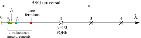
Figure 1: Out-of-equilibrium investigations of the BSG model. The BSG model describes the (low energy) universal features (i.e. independent of the microscopic details) of realistic situations when $\lambda\leq 3$. Crosses indicate the diagonal BSG models $\lambda\in\mathbb{N}$ which were up to now the only out-of-equilibrium solvable pointsFLS-PRL . The present work addresses the off-diagonal case $\lambda\notin\mathbb{N}$. Coloured circles indicate values for which transport experimental dataAnthore18 is available. We mention that there are also available transport measurements at $\lambda=2$ in the $\nu=1/3$ FQHE Saminadayar1997 .

Second, is a remarkable fact that as of today, excluding interacting systems that are unitarily related to free systemsSchillerHershfieldFreeSystems ; KomnikGogolin03 ; SelaAffleck09 , the only genuinely interacting system for which there is an exact solution yielding explicitly the out-of-equilibrium universal scaling functions say for the current, is the diagonal BSG model FLS-PRL ; FLS-PRB ; Bazhanov99 ; NoteSDIRLM ; Boulat08 defined by very specific values of the SG parameter ($\lambda$ an integer) where the system enjoys additional symmetries. More than 20 years after this breakthrough, the general solution of the out-of-equilibrium BSG away from diagonal points (defining the off-diagonal regime), is still missing (see Fig.1).

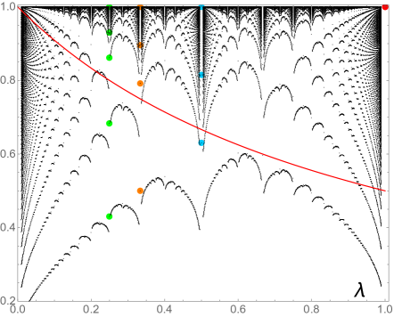
Figure 2: [Black] Normalized cumulative plot ($x_{a}=\frac{N_{a}}{\sum_{b}N_{b}}$) of the number $N_{a}(V,T,\lambda)$ of quasiparticles of type “$a$” involved in the exact description (shown here at vanishing bias voltage) as a function of the rational SG parameter $\lambda=\frac{{\mathfrak{p}}}{{\mathfrak{q}}}\leq 1$ with ${\mathfrak{q}}<100$. Note the very complex, self-similar structure that develops. Colored bullets emphasize the data at values $\lambda=\frac{1}{2},\frac{1}{3},\frac{1}{4}$ where our theory successfully accounts for the experimental data of Ref.Anthore18 , see section V. In spite of this complicated structure, interactions and the charge ${\mathfrak{q}}$ of the quasiparticles combine to yield perfectly regular transport properties when $\lambda$ is varied, e.g. the large temperature conductance $\frac{h}{e^{2}}\,G_{\rm max}=\frac{1}{\lambda+1}$ of the BSG model [Red, same dimensionless scale].

In this paper, motivated by recent high-precision measurements of the transport properties of chiral TLL Anthore18 , we present an exact solution when $\lambda$ is an arbitrary rational number giving access to the exact universal scaling function for the conductance at arbitrary voltage and temperature. Our solution proceeds in exploiting an equivalence (see Fig.3) between the original gas of QPs with off-diagonal scattering (that leads to charge diffusion in momentum space), and a gas involving exotic QPs diagonalizing charge transport, namely the string solutions of the XXZ modelTakahashi72 ; TakahashiBook whose number, nature and charge depend in a subtle way on the BSG parameter $\beta$ (see Fig. 2): for example the charge of the QPs is an everywhere discontinuous function of $\beta$.

This article, in addition to exposing the exact solution to the out-of-equilibrium BSG model, aims at giving the opportunity to the non-specialist reader to grasp the spirit of the solution in spite of complicated technicalities. The paper is organized as follows: in Section II, we sketch the main features of the solution and give the main results, deferring all the technical details to the subsequent sections. In Section III, after motivating their origin, we present the strings and spend some time gathering known results to present the (bare and dressed) basis of QPs and their thermodynamical properties. In Section IV we establish the main features of the impurity scattering in the string basis and we derive exactly the QP transmission probability using the boundary Yang Baxter equation and a Loschmidt echo. Finally in Section V we discuss our solution and present its remarkable agreement with recent experimental data for the tunnelling in a resistive environnement.

II Description of main results

II.1 The model, obstacles and route towards its solution

The boundary sine Gordon (BSG) model is defined by its Hamiltonian:

$$H_{\mbox{\scriptsize BSG}}=H_{0}+H_{\textsc{b}}$$ (2)

$$H_{0}=\hbar v_{\textsc{f}}\int_{-\infty}^{\infty}dx(\partial_{x}\phi)^{2}\,;\;\;H_{\textsc{b}}=\gamma\cos(\beta\phi(0))$$

It describes a free, chiral (right-moving) one-dimensional boson $\phi(x-t)$ defined on the whole line $x\in]-\infty,+\infty[$, the non-linear SG interaction $H_{\textsc{b}}$ acting as an impurity at $x=0$. The model is forced out-of-equilibrium by a constant voltage $\frac{eV}{2}\int dx\,Q(x)$ and we choose to normalize the charge density as

$$Q(x)=\frac{\beta}{2\pi}\,\partial_{x}\phi,$$ (3)

ensuring that the fundamental soliton of the SG model carries charge unityNoteChargeNormalization . The parameter $v_{\textsc{f}}$ sets the velocity scale of the problem. The parameter $\beta$, that fixes the period of the impurity potential, also determines the scaling dimension $\frac{\beta^{2}}{8\pi}=\frac{1}{\lambda+1}$ of the impurity perturbing operator, the later being relevant when $\beta<\sqrt{8\pi}$ or $\lambda>0$. The strength $\gamma$ of the impurity coupling generates a typical energy scale, the “impurity temperature” $T_{\textsc{b}}\propto\gamma^{\frac{\lambda+1}{\lambda}}$ that encapsulates all the microscopic, non-universal details of the problem (coupling strengths of possible additional irrelevant operators, e.g. band curvature, high-energy cut-off…) in a realistic situation. Note that when $\beta<\sqrt{2\pi}$, the operator $\cos(2\beta\phi(0))$ becomes relevant ; moreover, as being essentially the square of $H_{\textsc{b}}$, it is allowed by symmetries: therefore it is present, generates a new scale $T_{\textsc{b}}^{(2)}$ and universality is lost, defining the universal regime $\lambda\in[0,3]$.

It is clear that the BSG model (2) defines a scattering problem: given an arbitrary many-body state $\left|\psi\right\rangle_{\mbox{\scriptsize in}}$, incoming on the far left of the impurity, what is the final, outgoing state $\left|\psi\right\rangle_{\mbox{\scriptsize out}}$ on the far right? The central object encoding the physics is the scattering matrix ${\cal R}$, defined by $\left|\psi\right\rangle_{\mbox{\scriptsize out}}={\cal R}\left|\psi\right\rangle_{\mbox{\scriptsize in}}$. The scattering matrix ${\cal R}$ is a many-body object, and the non-linear character of $H_{\textsc{b}}$ forbids any simple description of the scattering in the basis of elementary excitations of the free boson $\phi(x)$ (see left column of Table 1).

$\color[rgb]{1,0,0}\hskip 45.52458pt\overset{\rm{\bf B.A.}}{\bm{\Longrightarrow}}\hskip 43.81705pt\overset{\rm{\bf A.B.A.}}{\bm{\Longrightarrow}}\color[rgb]{0,0,0}$
Basis free boson $\phi(x)$ (anti)solitons $\SS{\pm}(\theta)$ solitons/strings ${A}_{a}(\theta)$ Bulk scattering trivial factorized off-diagonal factorized diagonal Impurity scattering many-body factorized factorized

Table 1: Three different many-body basis for representing the BSG model. Gray boxes highlight an obstruction to the exact solution. The last column allows for an exact solution of the finite temperature BSG model out-of-equilibrium for arbitrary rational SG parameter $\lambda$, whereas the central one suffices for the diagonal case $\lambda$ integer.

The central idea to solve the problem is to identify a basis for many-body states built on QPs that diagonalizes the impurity scattering matrix ${\cal R}$. This will be done by exploiting the integrability of the BSG modelGhoshal94 to identify QP modesZamolodchikov79 , with specifically the following properties: $(i)$ the thermal gas of bosons (i.e. the finite temperature and voltage density matrix) incoming towards the impurity, can be represented in the QP basis ; $(ii)$ the QPs interact but the resulting scattering between QPs is factorized, with no particle production ; $(iii)$ the scattering of QPs on the impurity is factorized, with no particle production.

Introducing the symbol ${A}_{a}(\theta)$ to represent a QP mode with quantum number $a$, where the rapidity $\theta$ parametrizes the momentum $p\propto e^{\theta}$, point $(i)$ means that a many-body basis for the many-body Hilbert space $\mathscr{H}$ of bosons is made of Fock states: $\left|\psi\right\rangle=\prod_{i}{A}_{a_{i}}(\theta_{i})\left|0\right\rangle$ where $\left|0\right\rangle$ is the many-body vacuum and that the states $\left|\psi\right\rangle$ are suited for implementing the Thermodynamical Bethe Ansatz (TBA)Zamolodchikov90 allowing for a finite temperature $T$ and finite voltage $V$ description of the interacting QP gas. Point $(ii)$ means that the interaction amongst arbitrary colliding many-body states can be decomposed into elementary two-QP scattering processes ${A}_{a_{1}}(\theta_{1}){A}_{a_{2}}(\theta_{2})\longrightarrow{A}_{b_{2}}(\theta_{2}){A}_{b_{1}}(\theta_{1})$ the amplitude of this process being given by the bulk scattering matrix $S_{a_{1},a_{2}}^{b_{1},b_{2}}(\theta_{1}-\theta_{2})$. Third $(iii)$, factorization of the impurity scattering means that the latter can be described by a one-body scattering matrix $R_{ab}$, in the sense that ${\cal R}\left|\psi\right\rangle=\sum_{b_{1},b_{2},...}\prod_{i}R_{a_{i},b_{i}}(\theta_{i}){A}_{b_{i}}(\theta_{i})\left|0\right\rangle$, i.e. the QPs scatter one by one on the impurity with no QP production.

In the case of the BSG, the QPs fulfilling points $(\!ii\!\!-\!\!iii)$ have been identified by Goshal and Zamolodchikov Ghoshal94 as the solitons and antisolitons $\SS{\varepsilon}(\theta)$ of the SG modelZamolodchikov79 where $\varepsilon=\pm$ is a charge quantum number (center column of table 1). This QP basis has lead to the solutionFLS-PRB ; FLS-PRL of the diagonal BSG model ($\lambda\in\mathbb{N}$) out-of-equilibrium. For those exceptional values, the scattering amongst the QPs is diagonal or “reflectionless” (the process $\SS{+}(\theta_{1})\SS{-}(\theta_{2})\longrightarrow\SS{+}(\theta_{2})\SS{-}(\theta_{1})$ is forbidden) ensuring that point $(i)$ is satisfied.

However, in the generic case $\lambda\notin\mathbb{N}$ the scattering is off-diagonal meaning that solitons and antisolitons can exchange their quantum numbers during a scattering event, leading to diffusion of the soliton charge in momentum space (see Fig.3 [Top] and [Bottom Left]). As a consequence the (anti)solitons do not fulfill point ($i$), and one faces a major difficulty: that of finding yet another many-body basis allowing for the finite $T,V$ description of the QP gas and for the exact description of its scattering on the impurity. The Algebraic Bethe Ansatz (ABA) technique Takahashi72 ; TakahashiBook ; Fendley92 ; KorepinBook ; FaddeevHouches circumvents the issue of diffusion and furnishes a QP basis in which scattering becomes diagonal (third column of table 1). ABA therefore yields an equivalence between the original soliton/antisoliton gas with off-diagonal scattering, and a gas of new QPs with diagonal scattering, fulfilling point ($i$-$ii$) (see Fig.3[Bottom Right]). We then show that this basis fulfils point ($iii$) and derive exactly the impurity scattering in this new basis to complete the toolbox for the exact out-of-equilibrium solution.

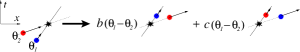
OR: 

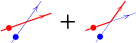
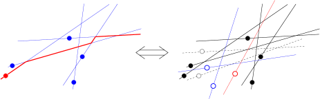
Figure 3: [Top] Illustration in the ($x,t$) plane of the off-diagonal scattering of solitons/antisolitons ( / ) $\SS{\pm}$ of the SG model with rational parameter $\lambda=\frac{{\mathfrak{p}}}{{\mathfrak{q}}}$. The trajectories have slopes $\propto e^{\theta}$ and in the short-hand notation [Right] the colour indicates the value of the charge quantum number $\varepsilon=\pm$. $b$ and $c$ are scattering amplitudes. [Bottom] Equivalence between a gas [Left] of solitons/antisolitons with off-diagonal scattering (note that only one of the many ”diffusive” trajectories of the soliton has been represented) and a gas [Right] of new quasiparticles ${A}_{a}$ with diagonal scattering, i.e. all quantum numbers $a$ (or colours) follow straight lines. In this equivalence the original SG soliton/antisoliton becomes a neutral soliton ${A}_{s}$ () carrying the energy, whereas new QPs emerge (open circles): two strings ${A}_{c}^{\pm}$ carrying charge $\pm{\mathfrak{q}}$ ( / ), and additional neutral strings (for the case $\lambda=\frac{1}{3}$ illustrated here, a single string ${A}_{1}$ (), see Appendix VII.1.1 for details). Whereas the total number $N_{a}$ of excited strings is fixed by the thermodynamics of the gas, the equivalence preserves $N_{{\includegraphics[width=5.12149pt]{SymbolSolPlus.pdf}}}+N_{{\includegraphics[width=5.12149pt]{SymbolSolMoins.pdf}}}=N_{{\includegraphics[width=5.12149pt]{SymbolSolABA.pdf}}}$ and $N_{{\includegraphics[width=5.12149pt]{SymbolSolPlus.pdf}}}-N_{{\includegraphics[width=5.12149pt]{SymbolSolMoins.pdf}}}={\mathfrak{q}}\big{(}N_{{\includegraphics[width=5.12149pt]{SymbolStringPlus.pdf}}}-N_{{\includegraphics[width=5.12149pt]{SymbolStringMoins.pdf}}}\big{)}$.

II.2 Main results

In order to solve the BSG model out-of-equilibrium, two different kinds of data is needed: first, the QP content and the thermodynamics of those QPs representing the (voltage biased) free boson gas incoming towards the impurity: this is reviewed in section III ; second, the impurity scattering matrix $R_{ab}$ of those QPs ; our original derivation is presented in section IV.

The particular value $\lambda=1$ of the SG parameter (1), where the model can mapped onto free fermions KaneFisher92 , marks the boundary between the repulsive ($\lambda<1$) and the attractive ($\lambda>1$) regime of the SG model. The attractive regime is characterized by the appearance of neutral soliton-antisoliton bound states (breathers), in the spectrum. In order to keep the presentation simple as possible, we focus here on the repulsive case that retains the full richness of the solution, while deferring the attractive case to Appendix VII.6. We also illustrate what needs to be done in pratice to obtain the current $I(V,T)$ in two specific examples $\lambda=\frac{1}{3}$ and $\lambda=\frac{6}{19}$ in Appendix VII.1.

For arbitrary rational $\lambda$ one introduces the continued fraction:

$$\lambda=\frac{{\mathfrak{p}}}{{\mathfrak{q}}}=\frac{1}{\nu_{1}+\frac{1}{\nu_{2}+...+\frac{1}{\nu_{\alpha}}}},$$ (4)

where $\nu_{i}$ are strictly positive integers ($\nu_{\alpha}>1$). The decomposition (4) is unique ContinuedFractions . Introducing the integers

$$m_{0}=0\;\;;\;\;m_{i}=\sum_{i^{\prime}=1}^{i}\nu_{i^{\prime}}\quad(i\leq\alpha),$$ (5)

there are in total ${m_{\alpha}}+1$ different kinds of QPs, whose creation operator is denoted ${A}_{a}(\theta)$ where the quantum number (or “species”) $a\in\{s,1,2,...,{m_{\alpha}}\}$.

The first particle ${A}_{s}$ is a neutral soliton, carrying kinetic energy, whereas the ${m_{\alpha}}$ other particles are massless particles (carrying no energy) called strings. All particles are neutral, except the last two ones ${A}_{{m_{\alpha}}}\equiv{A}_{c}^{+}$ and ${A}_{{m_{\alpha}}-1}\equiv{A}_{c}^{-}$, carrying $\pm{\mathfrak{q}}$ units of the SG-soliton charge. The main features of the QP spectrum are summarized in Table 2.

( particle	symbol	energy	charge	entropy
( soliton	${A}_{s}\equiv{A}_{0}$	✓	0	✓
neutral strings	$\begin{array}[]{c}{A}_{j}\\ {\mbox{\scriptsize$(1\!\leq\!j\!<\!{m_{\alpha}}\!\!-\!\!1)$}\vspace*{.1cm}}\end{array}$	.	0	✓
charged strings	$\begin{array}[]{l}{A}_{c}^{-}\equiv{A}_{{m_{\alpha}}\!-1}\\ {A}_{c}^{+}\equiv{A}_{{m_{\alpha}}}\vspace*{.1cm}\end{array}$	$\begin{array}[]{l}.\\ .\vspace*{.1cm}\end{array}$	$\begin{array}[]{l}-{\mathfrak{q}}\\ +{\mathfrak{q}\vspace*{.1cm}}\end{array}$	$\begin{array}[]{l}\checkmark\\ \checkmark\vspace*{.1cm}\end{array}$

Table 2: The dressed quasiparticle spectrum

The QPs can also be grouped in families $\big{(}{\cal F}_{i}\big{)}_{i=1...\alpha}$ characterized by distinct scattering properties. Each family ${\cal F}_{i}$ is made of the QPs $\big{(}{A}_{j}\big{)}_{m_{i-1}\leq j<m_{i}}$ (except for the last ${\cal F}_{\alpha}\!=\!\big{(}{A}_{j}\big{)}_{m_{\alpha-1}\leq j\leq{m_{\alpha}}}$) and each QP ${A}_{a}\in{\cal F}_{i}$ is assigned a sign $\eta_{a}=(-1)^{i+1}$.

The QPs have diagonal scattering and the thermodynamics of the QP gas at finite $T,V$ – i.e. precisely the density matrix describing our many-body system incoming towards the impurity – can be encoded by pseudoenergies $\epsilon_{a}(\theta)$, dimensionless functions that determine the total densities of QPs per unit length $\frac{k_{\textsc{b}}T}{hv_{\textsc{f}}}P_{a}(\theta)$ with $P_{a}=\eta_{a}\partial_{\theta}\epsilon_{a}$. The density of occupied particles per unit length is $\frac{k_{\textsc{b}}T}{hv_{\textsc{f}}}\rho_{a}(\theta)$ with $\rho_{a}=P_{a}f_{a}$ that also expresses as $\rho_{a}=-\eta_{a}\partial_{\theta}L_{a}$ with $L_{a}(\theta)=\ln(1+e^{\mu_{a}-\epsilon_{a}(\theta)})$, and $f_{a}=\frac{1}{1+e^{\epsilon_{a}(\theta)-\mu_{a}}}$ a Fermi function ; in view of Table 2 all (reduced) chemical potentials $\mu_{a}$ vanish except $\mu_{c}^{\pm}=\pm{\mathfrak{q}}\frac{eV}{2k_{\textsc{b}}T}$.

(i)aaaaaaaaaaaaaaaaaaaaaaaaaaaaaaaaaaaaaaaaaaaaaaa

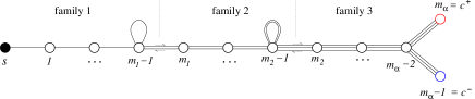
(ii.a)		$:\;\;\hat{K}_{a,b}=\hat{\Phi}^{\vphantom{\dagger}}_{p_{i}}\equiv\frac{1}{2\cosh(p_{i}\frac{\pi\omega}{2})}$
(ii.b)		$:\;\;\hat{K}_{b,a}=-\hat{K}_{a,b}=\hat{\Phi}^{\vphantom{\dagger}}_{p_{i}}$
(ii.c)		$:\;\;\hat{K}_{a,a}=\frac{\hat{\Phi}^{\vphantom{\dagger}}_{p_{i}}\hat{\Phi}^{\vphantom{\dagger}}_{p_{i+1}}}{\hat{\Phi}^{\vphantom{\dagger}}_{p_{i}-p_{i+1}}}$

Figure 4: (i) Dynkin diagram for the kernel $K_{ab}(\theta)$ entering the TBA equations, here depicted for $\alpha=3$, $(\nu_{1},\nu_{2},\nu_{3})=(4,3,4)$ (i.e. $\lambda=\frac{13}{56}$). The nodes represent the different kinds of particles: the massive soliton (black node) and a collection of massless strings (open nodes). The lines connecting the nodes encode non-vanishing entries of the kernel $K_{ab}$ made explicit in (ii). While most of the kernel is symmetric (ii.a), it also has non-symmetric entries (ii.b), as well as diagonal entries (ii.c).

The pseudoenergies obey a set of non-linear coupled integral equations, the TBA equations:

$$\epsilon_{a}=\delta_{a,s}e^{\theta}-\frac{1}{2\pi}K_{ba}\star L_{b}$$ (6)

where a sum over $b$ is implied, the convolution is defined as $(f\star g)(\theta)=\int_{-\infty}^{\infty}d\theta^{\prime}f(\theta^{\prime})g(\theta-\theta^{\prime})$, and the kernel entries $K_{ab}(\theta)$ (see Fig.4) are more conveniently given by their Fourier transforms $\hat{K}_{ab}(\omega)=\frac{1}{2\pi}\int_{-\infty}^{\infty}d\theta\,e^{-i\omega\theta}K_{ab}(\theta)$ in terms of elementary functions:

$$\Phi^{\vphantom{\dagger}}_{p_{i}}(\theta)=\frac{1/p_{i}}{\cosh(\theta/p_{i})}\quad\leftrightarrow\quad\hat{\Phi}^{\vphantom{\dagger}}_{p_{i}}(\omega)=\frac{1}{2\cosh(\frac{\pi p_{i}\omega}{2})}$$ (7)

where the numbers $p_{i}$ are defined by:

$$p_{0}=\lambda^{-1},\;\;p_{1}=1,\;\;p^{\vphantom{\dagger}}_{i>1}=p_{i-2}-\nu_{i-1}p_{i-1}.$$ (8)

The symmetry of the kernel apparent in Fig.4 implies that the two charged QPs share the same pseudoenergy $\epsilon_{c+}=\epsilon_{c^{-}}\equiv\epsilon_{c}$.

Our derivation of the impurity scattering matrix $R_{ab}(\theta)$ for the QPs ${A}_{a}(\theta)$ (see Section IV), completes the description, and allows to establish a universal formula for the current flowing through the impurity at arbitrary voltage and temperature, as a function of ${\overline{T}}=\frac{T}{T_{\textsc{b}}}$ and ${\overline{V}}=\frac{eV}{k_{\textsc{b}}T_{\textsc{b}}}$ (the boundary temperature $T_{\textsc{b}}$ was introduced below Eq. (3)) :

$$I(V,T) = \frac{({\mathfrak{q}}e)k_{\textsc{b}}T}{h}\,\int_{-\infty}^{\infty}\!\!\!d\theta\;{\cal T}_{\lambda}(\theta)\big{(}\rho_{c}^{+}(\theta)-\rho_{c}^{-}(\theta)\big{)},$$ (9)

$${\cal T}_{\lambda} = \frac{1}{1+\big{(}{\overline{T}}e^{\theta}\big{)}^{-2{\mathfrak{p}}}}\;\;;\;\;\rho_{c}^{\pm}=\frac{(-1)^{\alpha+1}\frac{\partial\epsilon_{c}(\theta)}{\partial_{\theta}}}{1+e^{\epsilon_{c}(\theta)\mp{\mathfrak{q}}\frac{\overline{V}}{2\overline{T}}}},$$

where ${\cal T}_{\lambda}(\theta)=|R_{c^{\pm},c^{\pm}}(\theta)|^{2}$ is the transmission probability of an incoming particle ${A}_{c}^{\pm}(\theta)$ through the impurity.

Although Eq. (9), that solve the BSG model out-of-equilibrium by yielding exactly the full universal scaling in the ($V,T$)-plane, look similar to those of the diagonal case $\lambda\in\mathbb{N}$ of Ref. FLS-PRB , it constitutes a novel prediction when $T\neq 0$. A first difference is that the involved QPs are now strings (and no longer solitons) carrying a non-trivial charge $\pm{\mathfrak{q}}$. Second, owing to our original derivation of the boundary scattering of strings, the transmission probability ${\cal T}_{\lambda}$ depends solely on ${\mathfrak{p}}$, the numerator of $\lambda$. Neither ${\mathfrak{q}}$ nor ${\mathfrak{p}}$ are smooth functions of $\lambda$, nor is the whole continued fraction representation (4) of the SG parameter that fixes the QP content and its scattering. Therefore the structure of Equations (6,9) for the pseudoenergies and the current is highly irregular when $\lambda$ is varied in sharp contrast with the behavior of physical quantities computed here that appear to be smooth functions of $\lambda$ (see Fig.2). As the simplest illustration, the expected high-energy limit of the conductance $G(V,T\gg T_{\textsc{b}})=\frac{e^{2}}{h}\frac{1}{\lambda+1}$ appears to be the result of a non-trivial calculation involving the complicated details of the QP spectrum when starting from our Eq. (10), see Appendix VII.5.2.

At small voltage, the scaling function for the linear conductance $G_{0}(T)\equiv\frac{\partial I(V,T)}{\partial V}\Big{|}_{V=0}$ can be expressed as:

$$G_{0}(T)=\frac{({\mathfrak{q}}\>e)^{2}}{h}\,(-1)^{\alpha}\!\!\int_{-\infty}^{\infty}d\theta\;{\cal T}_{\lambda}(\theta)\,\partial_{\theta}f_{c}(\theta)$$ (10)

where $f_{c}=f_{c^{+}}=f_{c^{-}}$ is the $V=0$ Fermi factor for the strings $A^{\vphantom{\dagger}}_{c}{\!{}^{\pm}}$. In particular, Eq.(10) predicts a universal temperature dependance in the linear regime $V\to 0$ that differs from the universal voltage dependance at $T=0$.

In the following, we work within units where $k_{\textsc{b}}=e=\hbar=v_{\textsc{f}}=1$, and sums over repeated indices are omitted.

III The quasiparticle basis

The quasiparticles ${A}_{a}$ involved in the exact out-of-equilibrium solution have their origin in the off-diagonal character of bulk scattering. To grasp how this can happen, let us consider the following simple situation: the scattering of a single soliton $\SS{+}(\theta)$ through a gas of $N$ antisolitons at rapidities $(\theta_{1},...,\theta_{N})$. In the diagonal case the soliton $\SS{+}(\theta)$ goes through the gas and just pick up a phase factor $Z(\{\theta_{i}\},\theta)=\prod_{i}S_{+-}^{+-}(\theta-\theta_{i})$, with $|Z|=1$. Off-diagonal scattering results in a final state which is a superposition of states where the positive charge can have moved at any rapidity $\theta_{i}$ simply by the off-diagonal process $\SS{+}(\theta)\SS{-}(\theta_{i})\to\SS{+}(\theta_{i})\SS{-}(\theta)$. The probability $|Z|^{2}=\prod_{i}|S_{+-}^{+-}|^{2}(\theta-\theta_{i})$ that the particle exiting the gas at rapidity $\theta$ is still the soliton is exponentially small in the number of antisolitons (since $|S_{+-}^{+-}|<1$). Hence with exponential precision the final wave function consists in states where an antisoliton $\SS{-}(\theta)$ exits leaving a positive charge $\SS{+}(\theta_{i})$ in the gas. This diffusion, in rapidity space, of the charge carried by solitons means that the soliton positive charge does not propagate in rapidity space through the antisoliton gas.

Obtaining the QP basis that allows to solve the off-diagonal BSG model requires the use of the Algebraic Bethe Ansatz method, that can be viewed as a (considerable) generalization of the preceding protocole, whereby ones send solitons at well chosen (complex) rapidities $\{\theta^{\prime}_{r}\}$ so that in the overall final state the charge distribution is unchanged and $Z(\{\theta_{i}\},\{\theta^{\prime}_{r}\})$ is again a pure phase shift. The additional rapidities organize into “strings” (a bunch of complex rapidities with given length $k$ centered around a real rapidity, defined in sections III.2.1 and III.2.2) that can be considered as genuine QPs, diagonalizing the problem of the aforementioned diffusion in many-body rapidity space. To do so, the rapidities $\{\theta^{\prime}_{r}\}$ are adjusted in a very precise way such that all the diffusive trajectories in many-body rapidity space interfere completely destructively, leading to diagonal bulk scattering in this new basis.

The string QPs are needed here to keep track of the reorganization of charge in rapidity space after each scattering event. As a matter of fact, those QPs carry only entropy (no energy nor momentum), and charge.

We first present the soliton/antisoliton basis that solves the problem in the diagonal BSG model. We then move on with the introduction of strings within ABA. Since some details will be crucial when introducing the impurity in Section IV, we review the main ingredients of this well known technique, by presenting the central idea of ABA (section III.2.1), then by introducing the “bare” strings (section III.2.2), and by finally presenting the “dressed” strings in Section III.2.3, and we also discuss some important features of the finite ($V,T$) thermodynamics of the QP gas in Section III.2.4.

III.1 Solitons and antisolitons

The basis factorizing the scattering amongst QPs and on the impurity can be identified by considering a massive generalization of the BSG model. It is convenient for this purpose to “fold” the model, defining a total (non-chiral) boson living on the semi-infinite line $x<0$, $\Phi(x)=\phi(x)+\phi(-x)$, as a sum of right- and left-moving bosons $\phi(x)$ and $\phi(-x)$ respectively BookDifrancesco ; BookTsvelikEtAl , which together with the boundary condition $\phi(0^{+})=\phi(0^{-})$ leads to:

$$H_{0} = \frac{1}{2}\int_{-\infty}^{0}dx\,{\cal H}_{0}(x)\;;\quad{\cal H}_{0}(x)=(\partial_{x}\Phi)^{2}+(\partial_{t}\Phi)^{2},$$

$$H_{\textsc{b}} = \gamma\cos(\frac{\beta}{2}\Phi(0)).$$ (11)

The well known trick FendleySaleurWarner is then to introduce a SG term ${\cal H}_{\mbox{\scriptsize SG}}(x)=\cos(\beta\Phi(x))$ in the bulk, replacing $H_{0}$ in (11) by $H_{0}^{M}=H_{0}+\Gamma\int_{-\infty}^{0}dx\,{\cal H}_{\mbox{\scriptsize SG}}(x)$. The resulting total Hamiltonian $H_{0}^{M}+H_{\textsc{b}}$, the massive BSG model, is integrable Ghoshal94 , with a QP content and bulk scattering matrix $S$ coinciding with that of the bulk sine-Gordon model defined of the full line with Hamiltonian $\int_{-\infty}^{\infty}({\cal H}_{0}+{\cal H}_{\mbox{\scriptsize SG}})$. In the repulsive regime $\lambda<1$, the QPs consist in a pair of massive solitons and antisolitons $\SS{\pm}(\theta)$, where the rapidity $\theta$ parametrizes the momentum $p=M\sinh\theta$ and energy $E=M\cosh\theta$ of the QPs, and $M$ is the mass gap of solitons. Then, the limit of vanishing $\Gamma$ (implying a vanishing mass gap $M\to 0$), is taken and the bulk part recovers its original nature of a free boson described by $H_{0}$. In the meantime, the rapidity is redefined $\theta\longrightarrow\theta+\ln\frac{2E_{0}}{M}$ where $E_{0}$ is an arbitrary reference energy scale (which we will later choose as $E_{0}=T$) so that the dispersion relation for QPs becomes that of massless particles, $E=p=E_{0}\,e^{\theta}$.

At the end of this procedure, one obtains a representation of the many-body Hilbert space of the original free boson (central column of Table 1) with basis the Fock states built with solitons $\SS{+}$ and antisolitons $\SS{-}$:

$$\left|\left\{\theta_{j},\varepsilon_{j}\right\}\right\rangle_{N}=\prod_{i=1}^{N}\SS{\varepsilon_{i}}(\theta_{i})\left|0\right\rangle\quad\varepsilon_{i}\in\{+,-\}$$ (12)

Our normalisation of the charge (3) ensures that the QPs $\SS{\pm}(\theta)$ carry charge $\pm 1$. The interaction amongst those QPs is encoded in the bulk scattering matrix $S$, defined by the relation $A^{\vphantom{\dagger}}_{\varepsilon_{1}}(\theta_{1})A^{\vphantom{\dagger}}_{\varepsilon_{2}}(\theta_{2})=S_{\varepsilon_{1}\varepsilon_{2}}^{\varepsilon^{\prime}_{1}\varepsilon^{\prime}_{2}}(\theta_{1}-\theta_{2})A^{\vphantom{\dagger}}_{\varepsilon^{\prime}_{2}}(\theta_{2})A^{\vphantom{\dagger}}_{\varepsilon^{\prime}_{1}}(\theta_{1})$. Charge symmetry leaves only few with non-zero entries Zamolodchikov79 :

$$S_{\pm\pm}^{\pm\pm}(\theta) = a(\theta)=e^{i\varphi_{z}^{\vphantom{\dagger}}(\theta)}$$ (13)

$$S_{\pm\mp}^{\pm\mp}(\theta) = b(\theta)=\frac{-\sinh(\lambda\theta)}{\sinh(\lambda(\theta-i\pi))}e^{i\varphi_{z}^{\vphantom{\dagger}}(\theta)}$$ (14)

$$S_{\pm\mp}^{\mp\pm}(\theta) = c(\theta)=\frac{-i\sin(\lambda\pi)}{\sinh(\lambda(\theta-i\pi))}e^{i\varphi_{z}^{\vphantom{\dagger}}(\theta)}$$ (15)

$$\varphi_{z}^{\vphantom{\dagger}}(\theta) = \int_{-\infty}^{\infty}\frac{d\omega}{2\omega}\sin(\omega\theta)\frac{\sinh\frac{\pi\omega(1-\lambda)}{2\lambda}}{\sinh\frac{\pi\omega}{2\lambda}\;\cosh\frac{\pi\omega}{2}}$$ (16)

For the integer SG model $\lambda\in\mathbb{N}$, the off-diagonal scattering amplitude vanishes, $c(\theta)=0$, resulting in the existence of an additional symmetry: not only the charge, and the individual momenta of the QPs are conserved during a scattering event, but also the momentum-resolved charge. It results that the $N$-particle states (12) are stable under (bulk) scattering, and therefore allow for a thermodynamical treatment of the gas of solitons/antisolitons in the grand-canonical ensemble, with micro-states of the form (12).

In the generic case with off-diagonal scattering $c(\theta)\neq 0$, this additional symmetry is absent: momentum and charge degrees of freedom are mixed by scattering leading to the aforedmentionned diffusion and the states (12) can no longer be used as the microstates of a thermodynamical treatement.

III.2 Solitons and strings

We now present the ABA approach, that allows to circumvent the off-diagonal character of the scattering and leads to the identification of the correct states, i.e. that are stable under bulk scattering (right-most column of table 1). Initially developed to solve the closely related XXZ model by Takahashi and coworkers Takahashi72 ; TakahashiBook ; KorepinBook ; FaddeevHouches , ABA has been implemented with success in the bulk SG model for various specific values of $\beta$ (see e.g. Refs Fowler82 ; Chung83 ; Fendley92 ; FendleySaleur94 ; Tateo95 ), but the results are somehow scattered in the literature. Moreover, the solution is presented in a variety of forms, sometimes making use of a remarkable identity leading to simplifications Zamolodchikov91 . We aim here at gathering all the information relevant for the derivation of the impurity scattering in Section IV, and at presenting a unified TBA system for arbitrary $\lambda\in\mathbb{Q}$. We also carefully derive the asymptotic behavior of the TBA equations when $\theta\to\pm\infty$.

III.2.1 Transfer matrix

Let us consider $\mathscr{H}^{\left\{\theta_{i}\right\}}$, the Hilbert space with $N$ particles (indifferently solitons or antisolitons) at rapidities $\left\{\theta_{i}\right\}_{i=1...N}$. A basis for $\mathscr{H}^{\left\{\theta_{i}\right\}}$ are the states (12) but due to non-diagonal scattering, the later are not stable under scattering and eigenvectors are to be sought in the more generic form:

$$\left|\Psi\right\rangle=\sum_{\varepsilon_{1},...,\varepsilon_{N}}\psi_{\varepsilon_{1},...\varepsilon_{N}}(\theta_{1},...\theta_{N})\left|\left\{\theta_{j},\varepsilon_{j}\right\}\right\rangle.$$ (17)

The allowed values for the rapidities $\left\{\theta_{i}\right\}$ are determined by a self-consistency condition: considering periodic boundary conditions and passing particle $k$ with rapidity $\theta_{k}$ through all others should leave the system invariant (up to a phase shift multiple of $2\pi$):

$$e^{ip^{\vphantom{\dagger}}_{j}L}\;\tau^{(s)}(\theta_{j})=e^{2i\pi{\cal N}_{s}(\theta_{j})}$$ (18)

where $p^{\vphantom{\dagger}}_{j}=E_{0}e^{\theta_{j}}$ is the momentum of particle $j$, $L$ is the size of the system, and the function ${\cal N}_{s}(\theta)$ takes integer values when $\theta=\theta_{j}$, an allowed rapidity. Equation (18) is the analog, for our gas of interacting particles where $\tau^{(s)}\neq 1$, of the usual quantization condition $e^{ipL}=1$ for a free gas in a box of size $L$.

In our case, off-diagonal scattering results in that the soliton transfer matrix $\tau^{(s)}(\theta)$ entering the quantization equation (18), is a $2^{N}\times 2^{N}$ matrix. First, the transfer matrix can be elegantly relatedFendley92 to the monodromy matrix $T_{\varepsilon}^{\;\varepsilon^{\prime}}(\theta)=\left(\!\!{\small\begin{array}[]{cc}A&B\\ C&D\end{array}}\!\!\right)$, where $A,B,C,D$ are $2^{N}\times 2^{N}$ $\theta$-dependent matrices, via (we make use of $\lim_{\theta\to 0}S_{\varepsilon_{1}\varepsilon_{2}}^{\varepsilon^{\prime}_{1}\varepsilon^{\prime}_{2}}(\theta)=\delta_{\varepsilon_{1}}^{\varepsilon^{\prime}_{2}}\delta_{\varepsilon_{2}}^{\varepsilon^{\prime}_{1}}$):

$$\tau^{(s)}(\theta)={\rm Tr}\big{(}T(\theta)\big{)}=(A+D)(\theta)$$ (19)

The monodromy matrix expresses the fate of a single particle with initial quantum number $\varepsilon\in\{+,-\}$ and rapidity $\theta$ passing through a bunch of $N$ particles with initial quantum numbers $\left\{c_{i}\right\}_{i=1...N}$ and rapidities $\left\{\theta_{i}\right\}$. It is a dynamical statement (time evolution of a particle scattering through a gas) that directly translates at the level of the solitons/antisolitons modes’ algebra as: $\SS^{\vphantom{\dagger}}_{\varepsilon}(\theta)\SS^{\vphantom{\dagger}}_{c_{1}}(\theta_{1})...\SS^{\vphantom{\dagger}}_{c_{N}}(\theta_{N})=\big{[}T_{\varepsilon}^{\;\varepsilon^{\prime}}\big{]}^{\{d_{i}\}}_{\{c_{i}\}}\SS^{\vphantom{\dagger}}_{d_{1}}\!(\theta_{1})...\SS^{\vphantom{\dagger}}_{d_{N}}\!(\theta_{N})\SS^{\vphantom{\dagger}}_{\varepsilon^{\prime}}(\theta)$. Explicitly, one has: $[T_{{\varepsilon}}^{\;\varepsilon^{\prime}}(\theta)]^{\left\{d_{i}\right\}}_{\left\{c_{i}\right\}}(\left\{\theta_{i}\right\})=\sum_{k_{1},...,k_{N-1}}S_{{\varepsilon}c_{1}}^{k_{1}d_{1}}(\theta\!-\!\theta_{1})\times S_{k_{1}c_{2}}^{k_{2}d_{2}}(\theta\!-\!\theta_{2})\ldots S_{k_{N-1}c_{N}}^{{\varepsilon^{\prime}}d_{N}}(\theta-\theta_{N})$. Coming back to our initial problem, the task of building the eigenfunctions $\psi$ in (17) requires diagonalizing the transfer matrix $\tau^{(s)}(\theta)$ at least for rapidities $\theta=\theta_{j}$. Remarkably, this can be done at any $\theta$ following the ABA method, yielding $\theta$-independent eigenvectors but $\theta$-dependent eigenvalues.

III.2.2 Bare strings

The essence of ABA is that eigenstates of $\tau^{(s)}(\theta)$ can be obtained by repeated applications of the $B$ matrix, evaluated at well chosen (complex) rapidities $\{\theta_{r}^{\prime}\}$, on the lowest state in $\mathscr{H}^{\left\{\theta_{i}\right\}}$ consisting of $N$ antisolitons:

$$\left|\Psi\{\theta^{\prime}_{r}\}\right\rangle = \prod_{r=1}^{N_{f}}B(\theta^{\prime}_{r})\left|\Omega\right\rangle,$$ (20)

$$\left|\Omega\right\rangle = \prod_{i=1}^{N}A^{\vphantom{\dagger}}_{-}(\theta_{i})\left|0\right\rangle.$$ (21)

The operator $B$, called the magnon operator, converts an antisoliton into a soliton and thus carries a charge $2$. Since we have $N_{f}$ flipped antisolitons, the charge of the state (20) is $Q=-N_{s}+2N_{f}$. The requirement that $\left|\Psi\{\theta^{\prime}_{r}\}\right\rangle$ be an eigenstate of $\tau^{(s)}$ results in that the rapidities $\{\theta^{\prime}_{r}\}$ are organized in so-called strings NoteCompleteness ; Hao13 . “Bare” strings of length $k$ with rapidity $\theta$ (as opposed to dressed ones, see Section III.2.4) will be denoted by $B_{k}(\theta)$ and consist in $k$ insertions of the magnon operator $B_{k}$ at $k$ different complex rapidities with common real part $\theta$ ; they are also characterized by a parity $\varepsilon=\pm 1$ Takahashi72 ; TakahashiBook :

$$\begin{array}[]{ll}B_{k}(\theta)=\prod_{\ell=1}^{k}B\big{(}\theta+i\frac{\pi(2\ell-k)}{2}\big{)}\hphantom{\;+\lambda^{-1}}&\varepsilon=+1\\ B_{k}(\theta)=\prod_{\ell=1}^{k}B\big{(}\theta+i\frac{\pi(2\ell-k+\lambda^{-1})}{2}\big{)}&\varepsilon=-1\end{array}$$ (22)

The allowed lengths $k_{j}$ are constrained by the normalizability of the wave function that leaves $n=m_{\alpha}$ strings with lengths (in the first line $j>0$ and $m_{i-1}\leq j<m_{i}$):

$$k_{j} = y_{i-2}+(j-m_{i-1})y_{i-1}$$ (23)

$$k_{{m_{\alpha}}} = y_{\alpha-1}$$ (24)

where the integers $y_{i}$ read:

$$y_{i}=y_{i-2}+\nu_{i}y_{i-1}\quad;\quad y_{-1}=0\;,\;y_{0}=1.$$ (25)

The parities are given by $\varepsilon_{m_{1}}=-1$ and otherwise $\varepsilon_{j}=(-1)^{[\lambda(k_{j}-1)]}$.

Strings do interact with each other and with solitons; the scattering matrix is diagonal (to simplify notations we introduce $S_{ab}\equiv S_{ab}^{ab}$) and is given by ($j,j^{\prime}\in\{1,...,{m_{\alpha}}\}$ are string indices):

$$S_{s,j}(\theta) = g_{-k_{j}}^{(\varepsilon_{j})}(\theta)$$ (26)

$$S_{1,j}(\theta) = g_{k_{j}+1}^{(\varepsilon_{j})}(\theta)g_{k_{j}-1}^{(\varepsilon_{j})}(\theta)$$

$$S_{j,j^{\prime}}(\theta) = \prod_{\ell=1}^{k_{j}}S_{1,j^{\prime}}\big{(}\theta+i\frac{\pi}{2}(k_{j}+1-2\ell)\big{)}$$ (27)

with the functions $g$:

$$g^{\!(\!+\!)}_{k}\!(\theta)=\frac{\sinh\lambda(\theta-\frac{ik\pi}{2})}{\sinh\lambda(\theta+\frac{ik\pi}{2})}\;;\;g^{\!(\!-\!)}_{k}\!(\theta)=g^{\!(\!+\!)}_{k}\!(\theta+\textstyle{\frac{i\pi}{2\lambda}}).$$ (28)

The (now diagonal) scattering data (26,27), together with (13), allows to derive in a standard way the Bethe equations defining the allowed rapidities for solitons and strings (see Appendix VII.2.1), which become after a continuum limit where the number of particles per unit length is sent to infinity:

$$\tilde{\eta}_{a}\,P_{a}=\delta_{a,s}e^{\theta}+\frac{1}{2\pi}\Phi_{a,b}\star\tilde{\rho}_{b}$$ (29)

where $\tilde{\eta}_{a}=-\eta_{a}\,(-1)^{\delta_{a,s}+\delta_{a,{m_{\alpha}}}}$ are some signs required to have a positive total density. Here the density of occupied QP (solitons or bare string) of type $a$ per unit length is written $\frac{T}{2\pi}\rho_{a}$, and $\frac{T}{2\pi}P_{a}$ is the total (occupied and empty) density of allowed QP rapidities.

III.2.3 Dressing

The complicated structure of the scattering (26,27) (all QPs scatter non-trivially with all QPs) can be greatly simplified by performing a dressing operation consisting in a particle-hole transformation on all strings but the last one, defining the dressed modes ${A}_{a}(\theta)$ (third column of Table 1). The dressing also has the advantage to reveal reveal a simple implementation of the U(1) charge symmetry of the QP gas, facilitating the coupling to an external bias voltage to later address non-equilibrium transport. Technical details about the dressing can be found in Appendix VII.2.

We check that after dressing the continuous Bethe equations relating $\frac{T}{2\pi}P_{a}(\theta)$, the total density (per unit length) of allowed rapidities for the modes ${A}_{a}(\theta)$ ($a=s,1,...,{m_{\alpha}}$), to $\frac{T}{2\pi}\rho_{a}(\theta)$, the QP density (per unit length) of occupied allowed rapidities, become:

$$P_{a}(\theta)=\delta_{a,s}e^{\theta}+\frac{1}{2\pi}\,\big{(}K_{ab}\star\rho_{b}\big{)}(\theta),$$ (30)

where the kernel $K_{ab}(\theta)$ is made explicit in Fig. 4. Note that the source term $\propto e^{\theta}$ is present for solitons only, indicating that strings carry no momentum nor kinetic energy.

The dressing operation affects not only the scattering properties, but also the charge quantum number of the QPs. One checks (see Appendix VII.2.3) that the dressed modes are neutral except for the last two dressed strings ${A}_{{m_{\alpha}}}\equiv{A}_{c}^{+}$ and ${A}_{{m_{\alpha}}-1}\equiv{A}_{c}^{-}$, carrying respectively $\pm{\mathfrak{q}}$ units of the original soliton $\SS{+}$. The features of the QP spectrum at arbitrary $\lambda\in\mathbb{Q}$ are summarized in Table 2.

III.2.4 Thermodynamics of the QP gas

The thermodynamics of this gas of interacting QPs is then derived in a standard way leading to the TBA (Thermodynamical Bethe Ansatz) equations Zamolodchikov90 that we already gave in Eq. (6). One can check explicitly (see Appendix VII.4.1) that the complicated description of the original free boson gas at finite $(V,T)$ in terms of the new QP modes, is exact, in the sense that the finite $V,T$ partition functions do coincide in the thermodynamical limit, providing an a posteriori check of the thermodynamical completeness of the soliton/string basis.

A few remarks are in order regarding those exotic QP modes ${A}_{a\neq s}$. Physically, those modes have their origin in the mixing of charge and momentum degrees of freedom that the original solitons/antisolitons experience due to off-diagonal scattering. It results that the modes ${A}_{a\neq s}$ are purely entropic: they do not carry energy (the later being carried only by solitons) but solely entropy that we can interpret as connected to the redistribution of the charge degrees of freedom after each off-diagonal scattering event.

In the limit of vanishing temperature, where only original solitons modes $\SS{+}$ (for positive voltage $V$) are occupied and the scattering effectively becomes diagonalFLS-PRL ; FLS-PRB (only the matrix element $S_{++}^{++}$ is involved, see Eq. (13)), the entropic QPs become frozen and, we can check, as illustrated in Fig. 5, that the solitons carry all the entropy (see Appendix VII.4.2). Formally, the freezing of the entropic QPs in this limit results in all the densities $\rho_{a\neq s}(\theta)$ being linearly determined by the soliton density $\rho_{s}(\theta)$ (see Eq. (40)).

In the opposite limit $V/T\ll 1$ the strings’s entropy $S_{a}(V,T)$ is at its highest, and reaches (see Appendix VII.4.2) a universal limit that remarkably does not depend on $\lambda$:

$$\frac{hv_{\textsc{f}}}{k_{\textsc{b}}T}\sum_{a=1}^{{m_{\alpha}}}\frac{S_{a}(0,T)}{k_{\textsc{b}}L}=2\mbox{Li}_{2}\Big{(}\frac{1}{4}\Big{)}+\ln 4\ln\frac{4}{3}\simeq 0.934...$$ (31)

where $\mbox{Li}_{2}(x)$ is the polylogarithm.

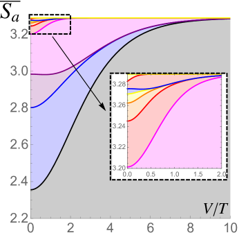
Figure 5: Cumulative plot of the dimensionless entropy per unit length $\overline{S}_{a}=\frac{hv_{\textsc{f}}}{k_{\textsc{b}}^{2}T}\frac{S_{a}}{L}$ carried by the $10=3+6+1$ QPs ($a=s,1,...,7,c^{-},c^{+}$ from bottom to top) as a function of $V/T$, for $\lambda=\frac{6}{19}=\big{(}3+\frac{1}{6}\big{)}^{-1}$ ; the inset is a zoom. The total entropy $\sum_{a}\overline{S}_{a}=\frac{\pi^{2}}{3}$ matches that of the original free boson gas. Note the vanishing of $\overline{S}_{a\neq s}$ in the low temperature limit where strings freeze and the soliton carries all the entropy.

The complex structure of the QP spectrum when $\lambda$ is varied is illustrated in Fig.2 where we display the fraction $x_{a}(\lambda,\frac{V}{T})=\frac{N_{a}(\lambda,\frac{V}{T}}{\sum bN_{b}(\lambda,\frac{V}{T})}$ of occupied QPs in the finite $T$ description (see Appendix VII.4.3 for the explicit calculation of the number of occupied particles $N_{a}(\lambda,\frac{V}{T})$). It is sometimes advocated that the strings are not QPs in the strict sense. We believe that this statement applies to the dressed description, but not to the bare one. The dressing operation, although drastically simplifying the structure of both the scattering and the charge carried by strings, comes with a (double) price: first, the TBA equations have a non-symmetric kernel, and second, the charge density of the dressed modes ${A}_{a}(\theta)$ (even of the neutral ones) is not localized but has some spreading in rapidity space (see Appendix VII.2.3), making the modes ${A}_{a}(\theta)$ rather unconventional. However, in the bare soliton/strings basis, the modes $B_{k_{j}}(\theta)$ have diagonal, symmetric scattering, and possess all the features of ”usual” QPs: they are localized in momentum space, carry some entropy (but oddly no energy). Ultimately, the physical meaning of these strings is clear: they are ”book-keeping” particles (hence their entropic character) that are necessary to account for the diffusion in momentum space experienced in the original (anti)soliton basis.

IV Impurity scattering

In this section we derive the structure of the impurity scattering matrix for the QPs. We note that it was derived, in the particular (off-diagonal) case where $\lambda^{-1}$ is an integer, in Ref. FendleySaleur94 , but in the different case where the boson $\phi$ has fixed boundary conditions. We need here the general case $\lambda\in\mathbb{Q}$ and free boundary conditions, which, as far as we know, has not been considered. After constraining the structure of the $R-$matrix in Section IV.1 we will relate the scattering in the original soliton/antisoliton, and in the dressed QP basis in Section IV.2 and derive the exact transmission probability of charged strings when crossing the impurity.

The SG model with impurity being integrableGhoshal94 , it results that the scattering over the impurity in the BSG model (2) factorizes, i.e. it can be decomposed as a product of elementary one QP processes. Formally, this is described by introducing the (many-body) impurity scattering matrix ${\cal R}$. This object relates (incoming) states on the left of the impurity, built out of the modes ${A}_{a}^{\mbox{\scriptsize in}}(\theta)$, to (outgoing) states living on the right of the impurity and built out of the modes ${A}_{a}^{\mbox{\scriptsize out}}(\theta)$. Then, factorization means that a generic incoming state $\left|\psi\right\rangle_{\mbox{\scriptsize in}}=\prod_{i=1}^{N}{A}_{a_{i}}^{\mbox{\scriptsize in}}(\theta_{i})\left|0\right\rangle$ ($\left|0\right\rangle$ is the many-body vacuum) will evolve into a new state $\left|\psi\right\rangle_{\mbox{\scriptsize out}}={\cal R}\left|\psi\right\rangle_{\mbox{\scriptsize in}}=\sum_{b_{1},b_{2},...}\prod_{i=1}^{N}R_{a_{i},b_{i}}(\theta_{i}-\theta_{\textsc{b}}){A}_{b_{i}}^{\mbox{\scriptsize out}}(\theta_{i})\left|0\right\rangle$ where $R_{ab}$ is the one-body impurity scattering matrix, and the dependence on the energy scale $T_{\textsc{b}}$ generated by the impurity interaction is simply encoded in $\theta_{\textsc{b}}$, the impurity rapidity defined by $\theta_{\textsc{b}}=\log(T_{\textsc{b}}/T)$. The one-body impurity scattering matrix $R_{ab}$, describing the fate of a single incoming QP with quantum number $a\in\{+,-\}$ is well known in the soliton/antisoliton basis. Since the impurity interaction term $H_{\textsc{b}}$ in Eq. (2) does not conserve charge, it is a $2$ matrix over the soliton-antisoliton space (at fixed rapidity) ; charge conjugation symmetry implies that it has only two distinct elements $R_{\pm\pm}=P$ and $R_{\pm\mp}=Q$, that are given by Ghoshal94 ; FendleySaleurWarner :

$$P^{(\lambda)}(\theta) = \frac{e^{\lambda\theta}}{1+ie^{\lambda\theta}}\;e^{i\varphi_{\textsc{b}}^{(\lambda)}}(\theta)$$

$$Q^{(\lambda)}(\theta) = \frac{i}{1+ie^{\lambda\theta}}\;e^{i\varphi_{\textsc{b}}^{(\lambda)}}(\theta)$$ (32)

$$\varphi_{\textsc{b}}^{(\lambda)}(\theta) = C_{\lambda}+\int_{-\infty}^{\infty}\frac{dt}{2t}\sin\Big{(}\frac{2\lambda\theta t}{\pi}\Big{)}\,\frac{\sinh((1-\lambda)t)}{\cosh(\lambda t)\sinh(2t)}$$

with $C_{\lambda}$ a constant that will not be needed here.

IV.1 Structure of the impurity scattering

However, what is needed here is the impurity scattering matrix ${\cal R}$ in the string/soliton basis. It is not obvious at all how to derive this object, since the strings are built out of the magnon operator $B(\theta)$ (flipping an antisoliton into a soliton) and not directly out of the soliton/antisoliton modes $\SS{\pm}(\theta)$. To this aim we compute a Loschmidt echo in both QP basis. We will see that this allows to determine the structure of ${\cal R}$, that also factorizes in the new string/soliton basis.

Integrability in the presence of an impurity demands that the impurity scattering $R$ is compatible with the bulk scattering $S$, i.e. the side of the impurity where the bulk scattering takes place does not matter. This requirement, the boundary Yang Baxter equationGhoshal94 , reads:
where in this graphical representation the impurity is figured by the red dashed line, and an empty (respectively full) circle stands for an insertion of the impurity scattering matrix $R$ (respectively bulk scattering matrix $S$). Repeated applications of the BYBE equation allow to derive a self consistency equation for the monodromy matrix $T_{a}^{\;b}$. It is more difficult to make mistakes when drawing this equation:

than when writing it down:

$$[T_{a}^{\;\;b^{\prime}}(\theta)]_{\{\alpha_{i}\}}^{\;\;\{\beta_{i}^{\prime}\}}{\cal R}_{\{\beta_{i}^{\prime}\}}^{\;\;\{\beta_{i}\}}(\theta_{\textsc{b}})R_{b^{\prime},b}(\theta-\theta_{\textsc{b}})=$$

$$R_{a,a^{\prime}}(\theta-\theta_{\textsc{b}}){\cal R}_{\{\alpha_{i}\}}^{\;\;\{\alpha^{\prime}_{i}\}}(\theta_{\textsc{b}})[T_{a^{\prime}}^{\;\;b}(\theta)]_{\{\alpha^{\prime}_{i}\}}^{\;\;\{\beta_{i}\}}.$$ (33)

Now from (33) we can derive four relations (by fixing the free indices $a,b$) which, combined together, yield $[A+D,{\cal R}]=\frac{P}{Q}[{\cal R},B+C]=\frac{Q}{P}[{\cal R},B+C]$ $\forall\,(\theta,\theta_{\textsc{b}})$, implying that all those commutators vanish. Remembering that $(A+D)(\theta)$ is nothing but the transfer matrix defined in (19), we arrive at:

$$[\tau^{(s)}(\theta),{\cal R}(\theta_{\textsc{b}})]=0.$$ (34)

A direct consequence of this equation is that all non-degenerate eigenstates of $\tau^{(s)}$ are eigenstates of ${\cal R}$. The non accidental degeneracies of the eigenvalues of $\tau^{(s)}$, for two different configurations $\mathscr{C}\neq\mathscr{C}^{\prime}$, are actually linked to the U(1) charge symmetry of the problem: it turns out that $S_{{m_{\alpha}}-1,a}(\theta)S_{{m_{\alpha}},a}(\theta)=1$, $\forall\,\theta\;,\forall\,a=s,1,...,{m_{\alpha}}$ (see Appendix VII.5.1). Hence a pair of the last two (bare) strings, $B_{k_{{m_{\alpha}}-1}}(\theta)B_{k_{{m_{\alpha}}}}(\theta)$, does not produce any scattering at all, i.e. it can be added or removed without affecting the quantization condition of the other QPs. More precisely, let us consider an allowed configuration $\mathscr{C}=\{\theta^{(a)}_{r}\}$, $a=s,1,...,{m_{\alpha}}$; $r=1...N_{a}$ with $N_{s}$ solitons, and $N_{j}$ insertions of strings of type $j$ in the state (20). Consider then a given rapidity $\theta_{0}$ that is doubly occupiedfootnoteDoubly for the last two strings, i.e. both strings $B_{k_{{m_{\alpha}}}}(\theta_{0})$ and $B_{k_{{m_{\alpha}}-1}}(\theta_{0})$ appear in the state (20). We can immediately deduce that the configuration $\mathscr{C}^{\prime}$ obtained from $\mathscr{C}$ by removing the pair $B_{k_{{m_{\alpha}}-1}}(\theta_{0})B_{k_{{m_{\alpha}}}}(\theta_{0})$ from the state (20), is (i) an allowed configuration and (ii) degenerate with $\mathscr{C}$ in the sense that they share the same $\tau^{(s)}(\theta)$ eigenvalue.

Moving towards the dressed picture and performing the particle-hole transformation, we can conclude that eigenvalues of the transfer matrix $\tau^{(s)}(\theta)$ are degenerate $\forall\,\theta$ for configurations that are obtained from each other by the conversion of an arbitrary number of occupied positive strings ${A}_{c}^{+}$ into (initially empty) negative strings ${A}_{c}^{-}$, and vice versa. From this analysis we can conclude that the structure of the one-particle dressed $R-$matrix is diagonal for all the neutral sector $a\in\{s,1,...,{m_{\alpha}}-2\}$, and consists of a $2\times 2$ block for the charged sector:

$$R_{a,a}(\theta) = e^{i\xi^{\vphantom{\dagger}}_{a}(\theta)}\quad{\rm if\;\;}a\neq c^{\pm},$$

$$R_{c^{\pm},c^{\pm}}(\theta) = P_{\rm dr}(\theta),$$

$$R_{c^{\pm},c^{\mp}}(\theta) = Q_{\rm dr}(\theta).$$ (35)

IV.2 Impurity scattering matrix for strings and solitons

We now determine the scattering data in (35), by translating the details of the impurity scattering (32) for solitons/antisolitons into the dressed ABA picture involving strings and solitons. To this end, we study the system with impurity chosing a particular many-body incoming state, namely the fully polarized state $|\Omega\rangle$ defined in (21). This situation physically corresponds to setting the temperature to zero with a finite negative voltage bias.

Let us prepare the system in the reference state $\left|\Psi\right\rangle_{0}=\left|\Omega\right\rangle_{\rm in}$, then evolve it in time until it has crossed the impurity so that it now consists of a many-body coherent superposition of outgoing modes (ending up in state $\left|\Psi\right\rangle_{\infty}={\cal R}\left|\Omega\right\rangle_{\rm in}$, where arbitrarily many $\SS{-}$ have been converted in $\SS{+}$ on the impurity), and finally project it onto the reference state $\left|\Omega\right\rangle_{\rm out}$. The overlap is a Loschmidt echo, and we define:

$${\cal L}=-\ln\big{[}\;^{\vphantom{\dagger}}_{\rm out}\!\langle\Omega\big{|}\Psi\rangle_{\infty}\big{]}.$$ (36)

Using the explicit form for the matrix ${\cal R}$ we want to evaluate ${\cal L}$ in the original soliton/antisoliton basis and in the dressed basis, therefore relating the impurity scattering in the two descriptions. In the original basis, since the incoming state is made of $N_{s}$ antisolitons, it is straightforward to evaluate the overlap in (36): it selects only the $R_{--}=P$ processes yielding:

$$e^{-{\cal L}}=\prod_{j=1}^{N_{s}}P(\theta_{j}-\theta_{\textsc{b}}).$$ (37)

Let us now turn to the dressed description. We first need to express the state $\left|\Omega\right\rangle$ in the new basis: at the bare level all strings are empty, so that after dressing by the particle-hole transformation, all QP modes ${A}_{a}$ with $a\neq s,{m_{\alpha}}$ are fully occupied and all modes ${A}_{c}^{+}$ are empty: $\left|\Omega\right\rangle=\prod_{i=1}^{N_{s}}{A}_{s}(\theta_{i}^{(s)})\prod_{j=1}^{{m_{\alpha}}-1}\prod_{r=1}^{N_{j}}{A}_{j}(\theta_{r}^{(j)})\left|0\right\rangle_{\rm dr}$ where the dressed vacuum $\left|0\right\rangle_{\rm dr}$ is defined in Eq.(58).

After scattering on the impurity, the state $\left|\psi\right\rangle_{\infty}$ still has all QP states of type $j<{m_{\alpha}}-1$ fully occupied, but some QPs ${A}_{c}^{-}$ have been converted into ${A}_{c}^{+}$. Projecting onto $\left|\Omega\right\rangle_{\rm out}$ selects the events $R_{c^{-},c^{-}}$ for all $\theta_{r}^{({m_{\alpha}}-1)}$ so that we get from (35) the following alternate form for the Loschmidt echo:

$$e^{-{\cal L}}=\prod_{r=1}^{N_{{m_{\alpha}}-1}}P_{\rm dr}(\theta_{r}^{({m_{\alpha}}-1)}-\theta_{\textsc{b}})$$

$$\times\prod_{j=1}^{{m_{\alpha}}-2}\prod_{r=1}^{N_{j}}e^{i\xi_{j}(\theta_{r}^{(j)}-\theta_{\textsc{b}})}\prod_{i=1}^{N_{s}}e^{i\xi_{s}(\theta_{i}^{(s)}-\theta_{\textsc{b}})}.$$ (38)

In the thermodynamical limit the system is described by the density of occupied antisolitons $\rho_{s^{-}}(\theta)$ in the bare description, or moving to the ABA basis, by densities of occupied solitons and strings $\rho_{j}(\theta)$. Note that since there are only antisolitons in $\left|\Omega\right\rangle$, one has $\rho_{s^{-}}=\rho_{s}$. It is actually more convenient to evaluate $\chi^{\vphantom{\dagger}}_{\textsc{b}}(\theta_{\textsc{b}})\equiv-\frac{i}{L}\partial_{\theta_{\textsc{b}}}{\cal F}$: introducing $\Phi_{\textsc{b}}^{(\lambda)}=-i\partial_{\theta}\ln P^{(\lambda)}$, $\Phi_{\textsc{b}}^{\rm dr}=-i\partial_{\theta}\ln P_{\rm dr}$, and Fourier transforming with respect to $\theta_{\textsc{b}}$ we obtain:

$$\hat{\chi}_{\textsc{b}}^{\vphantom{\dagger}}(\omega) = \hat{\rho}_{s}(-\omega)\hat{\Phi}_{\textsc{b}}^{(\lambda)}(\omega)$$

$$= \hat{\rho}_{c^{-}}(-\omega)\hat{\Phi}_{\rm dr}^{\textsc{b}}(\omega)+i\omega\!\!\!\!\!\!\sum_{a=s,1,...,{m_{\alpha}}-2}\!\!\!\!\!\!\hat{\rho}_{a}(-\omega)\hat{\xi}_{a}(\omega).$$

String bands being either full and empty (hence the entropy is totally fully carried by antisolitons, see fig. 5) in the state $\left|\Omega\right\rangle$, the string densities in the continuum limit satisfy $\rho_{j}(\theta)=P_{j}(\theta)$ $\forall j\notin\{s,{m_{\alpha}}\}$ and $\rho_{{m_{\alpha}}}(\theta)=0$. Moreover, they are not independent of each other: from (56) and using the relationship between bare and dressed densities, $\tilde{\rho}_{j}=P_{j}-\rho_{j}$ ($j\notin\{s,{m_{\alpha}}\}$) one gets $-2\pi\,\eta_{j}\,P_{j}=\Phi_{s,j}\star\rho_{s}$ ($j\neq s$) so that finally:

$$\hat{\rho}_{j}(\omega)=-\eta_{j}\,\hat{\Phi}_{s,j}(\omega)\,\hat{\rho}_{s}(\omega)\quad(1\leq j<{m_{\alpha}})$$ (40)

where $\Phi_{s,j}$ is the log derivative of the bare scattering (26).

Now focusing for a moment on the imaginary part of $\chi_{\textsc{b}}$, that is responsible for the decay of the Loschmidt echo, it receives contributions only from those entries of the $R-$matrix that have modulus $|R_{ab}|\neq 1$, that is, in the first line of Eq. (IV.2), from the modulus of the soliton transmission amplitude, and in the second line from the term $j={m_{\alpha}}-1$ involving the charged QP ${A}_{c}^{-}$. The explicit form for the bare scattering $\hat{\Phi}_{\textsc{b}}^{(\lambda)}$ that one deduces from (32):

$$\hat{\Phi}_{\textsc{b}}^{(\lambda)}(\omega)=-\frac{i\lambda}{2}\,\delta(\omega)+\frac{1-\tanh\frac{\pi\omega}{2}}{4\sinh\frac{\pi\omega}{2\lambda}},$$ (41)

combined with the relationship between densities (40) allow to derive a remarkable relation, relating the imaginary part of $\chi_{\textsc{b}}$ in the original soliton/antisoliton basis and in the dressed string/soliton basis:

$$\hat{\rho}_{s}(-\omega)\hat{\Phi}_{\textsc{b}}^{(\lambda)}(\omega)=\hat{\rho}_{c^{-}}(-\omega)\hat{\Phi}_{\textsc{b}}^{({\mathfrak{p}})}(\omega)$$ (42)

where one has used the soliton-charged string bare scattering $\hat{\Phi}_{s,c^{-}}=\hat{\varphi}_{-k_{{m_{\alpha}}-1}}^{(\varepsilon_{{m_{\alpha}}-1})}=(-1)^{\alpha}\frac{\sinh\frac{\pi\omega}{2{\mathfrak{p}}}}{\sinh\frac{\pi\omega}{2\lambda}}$ (as obtained from Eqs.(26,57) and the explicit parities for the charged strings, see Appendix VII.5.1).

Plugging (42) into Eq. (IV.2), we conclude that the dressed $R-$matrix can be written as:

$$R_{a,a}(\theta) = e^{i\xi_{a}(\theta)}\quad(a\neq c^{\pm}),$$

$$P_{\rm dr}(\theta) = P^{({\mathfrak{p}})}(\theta)\;e^{i\xi_{c}(\theta)},$$ (43)

$$Q_{\rm dr}(\theta) = Q^{({\mathfrak{p}})}(\theta)\;e^{i\xi_{c}(\theta)},$$

where $P^{({\mathfrak{p}})}(\theta)$ and $Q^{({\mathfrak{p}})}(\theta)$ are defined in (32) with the replacement $\lambda\to{\mathfrak{p}}$, i.e. the dressed $R-$matrix in the off-diagonal BSG model, up to phases, is essentially that of a diagonal BSG model: as far as impurity scattering is concerned, everything happens as if the SG parameter were renormalized to an integer value, $\lambda=\frac{{\mathfrak{p}}}{{\mathfrak{q}}}\longrightarrow{\mathfrak{p}}$. The phases $\xi_{a}(\theta)$, which we will not need in the following, are furthermore constrained by the relation:

$$\sum_{a=s,1,...,{m_{\alpha}}-2,c}\!\!\!\!\!\!\eta_{a}\;\hat{\Phi}_{a,s}(\omega)\;\hat{\xi}_{a}(\omega)=0.$$ (44)

IV.3 Rate equation for the current

With the dressed scattering (43) at hand, we can derive the exact transmission probabilities for the QPs, as a function of the rapidity and the impurity temperature $T_{\textsc{b}}$. As enforced by the degeneracies of the eigenvalues of the transfer matrix $\tau_{s}$, all neutral particles have transmission one (including the eventual breathers in the attractive case, see Appendix VII.6), while the charged strings ${A}_{c}^{\pm}(\theta)$ are transmitted with probability ${\cal T}_{\lambda}(\theta)=|R_{c^{\pm},c^{\pm}}(\theta-\theta_{\textsc{b}})|^{2}$ (and are scattered as the anti-QP ${A}_{c}^{\mp}$ with probability $1-{\cal T}_{\lambda}(\theta)$):

$${\cal T}_{\lambda}(\theta)=\frac{1}{1+\big{(}\overline{T}\,e^{\theta}\big{)}^{-2\hskip 0.28436pt{\mathfrak{p}}}}$$ (45)

Note that the apparent temperature dependence (we still have $\overline{T}=\frac{T}{T_{\textsc{b}}}$) observed in (45) is just an artefact of our choice of the arbitrary scale $E_{0}=T$ parametrizing momentum $p=Te^{\theta}$. A formula for the current can be established by evaluating the rate of change of the charge due to the scattering QPs, following closely the diagonal solutionFLS-PRB but with charged strings replacing solitons/antisolitons.

The charge $\delta Q=\delta Q_{+}+\delta Q_{-}$ flowing through the impurity during a time interval $\delta t$, receives contributions from positive strings ${A}_{c}^{+}(\theta)$ as well as negative strings ${A}_{c}^{-}(\theta)$ incoming towards the impurity at rapidity $\in[\theta,\theta+d\theta]$, that are both transmitted with probability ${\cal T}_{\lambda}(\theta)$. The number of incoming strings ${A}_{c}^{\pm}(\theta)$ during $\delta t$ being $\delta n^{\pm}(\theta)=(v_{\textsc{f}}\delta t)\frac{k_{\textsc{b}}T}{hv_{\textsc{f}}}\rho_{c}^{\pm}(\theta)d\theta$, the transmitted charge reads $\delta Q_{\pm}=(\pm{\mathfrak{q}}e)\times\delta n^{\pm}\times{\cal T}_{\lambda}$ leading to $\frac{\delta Q_{\pm}}{\delta t}=\pm\frac{{\mathfrak{q}}ek_{\textsc{b}}T}{h}\rho_{c}^{\pm}$, so that the total current $I=(\delta t)^{-1}\int d\theta(\delta Q_{+}-\delta Q_{-})$ finally evaluates to Eq. (9).

V Discussion

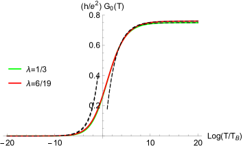
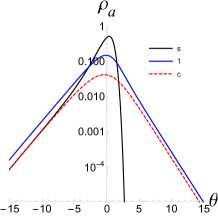
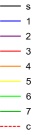
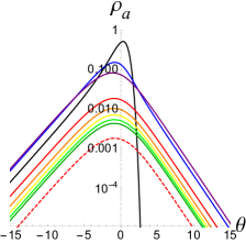
Figure 6: [Top] Universal scaling curves for the (reduced) linear conductance $\frac{h}{e^{2}}G_{0}(T/T_{\textsc{b}})$ obtained from Eq. (10), and shown here for $\lambda_{1}=\frac{1}{3}$ and $\lambda_{2}=\frac{6}{19}$, illustrating the smoothness of the conductance when $\lambda$ is varied. The dashed lines are the exact asymptotics (46) and (47). [Bottom] QP densities as a function of $\theta$, shown here at $V=0$, for the case $\lambda_{1}$ [Left] and $\lambda_{2}$ [Right]. For those two close values at relative distance $\frac{\lambda_{1}-\lambda_{2}}{\lambda_{1}}\simeq 0.053$, the QP contents from which the conductance is evaluated are largely different (see also Figs.8,9 in Appendix VII.1). Note in particular the different scales in the values of $\rho_{c}$, which decreases when the denominator ${\mathfrak{q}}$ increases.

Our prediction (9) for the finite voltage and temperature universal form of the current $I(V,T)$ allows for a certain number of checks. First, at vanishing temperature, as discussed in Section III.2.4, the strings freeze ; a possible description involving antisolitons only becomes possible, and our prediction coincides with the $T=0$ predictions of Ref. FLS-PRB exploiting the diagonal character of the scattering.

At finite temperature strings enter the stage and our prediction for the current is novel. A fist available benchmark is the high energy ($T\gg T_{\textsc{b}}$) limit of the the linear conductance $G_{0}(T)=\lim_{V\to 0}(\partial I(V,T)/\partial V)$, $G_{\mbox{\scriptsize max}}=\frac{e^{2}}{h}\frac{1}{\lambda+1}$. From Eq. (10) one gets $\frac{h}{e^{2}}G_{\mbox{\scriptsize max}}=(-1)^{\alpha}{\mathfrak{q}}^{2}[f_{c}]_{-\infty}^{\infty}$ and using the asymptotic values of the pseudoenergies, we show in Appendix VII.5.2 that $[f_{c}]_{-\infty}^{\infty}=\frac{(-1)^{\alpha}}{{\mathfrak{q}}^{2}(\lambda+1)}$. A second benchmark are the asymptotic regimes (large and small $\frac{T}{T_{\textsc{b}}}$) for the conductance, that read (see Appendix VII.7):

$$\frac{G_{0}(T)}{G_{\mbox{\scriptsize max}}} \underset{T\ll T_{\textsc{b}}}{\sim} \alpha^{\vphantom{\dagger}}(\lambda)\,\Big{(}B({\textstyle\frac{1}{2},1+\frac{1}{2\lambda}})\frac{T}{T_{\textsc{b}}}\Big{)}^{2\lambda},$$ (46)

$$\frac{G_{0}(T)}{G_{\mbox{\scriptsize max}}} \underset{T\gg T_{\textsc{b}}}{\sim} 1-\alpha^{\vphantom{\dagger}}({\textstyle\frac{-\lambda}{\lambda+1}})\,\Big{(}B({\textstyle\frac{1}{2},1+\frac{1}{2\lambda}})\frac{T}{T_{\textsc{b}}}\Big{)}^{{\textstyle\frac{-2\lambda}{\lambda+1}}}$$ (47)

where the coefficients read $\alpha^{\vphantom{\dagger}}(\lambda)=\frac{(\lambda+1)\Gamma(\lambda+1)^{2}B\big{(}\lambda+1,\frac{1}{2}\big{)}}{2}$ and $B(a,b)=\frac{\Gamma(a)\Gamma(b)}{\Gamma(a+b)}$ is the Euler beta function.

The linear conductance $G_{0}(T)$ is shown in the top panel of Fig.6 for two close values of the SG parameter $\lambda_{1}=\frac{1}{3}$ and $\lambda_{2}=\frac{6}{19}$ While the conductance varies smoothly between the two cases, the QP spectrum changes drastically. One observes that the last band $\epsilon_{c}$ corresponding to the charged particle flattens when the denominator ${\mathfrak{q}}$ increases and consequently $P_{c}$ and $\rho_{c}$ decrease. For large $V/T$ a simple charge counting argument leads to a reduction of the number of charged QP states scaling as ${\mathfrak{q}}^{-1}$, and at small $V/T$ we show in Appendix VII.5.2 that the number of charged QPs is even further reduced by an additional factor and scales as $\frac{1}{{\mathfrak{q}}^{2}}$, for large ${\mathfrak{q}}$ and typical fractions $\lambda$. This of course makes the approach to any given value $\lambda$ by a rational series $\lambda_{\ell}\underset{\ell\to\infty}{\longrightarrow}\lambda$ highly singular, the charge ${\mathfrak{q}}^{\vphantom{\dagger}}_{\ell}$ becoming infinitely large while the number of excited charged particles $N_{c}^{\pm}$ (at fixed $V,T$) goes to zero.

The number of such strings, or “book-keeping” particles (they keep track of the diffusion of charge in momentum space), turns out to be finite ($={m_{\alpha}}$) when $\lambda=\frac{{\mathfrak{p}}}{{\mathfrak{q}}}$ is a rational number, simply because then any scattering matrix element is periodic: $S(\theta+i{\mathfrak{q}}\pi)=S(\theta)$, implying that strings above a certain length (that scales as ${\mathfrak{q}}$) are not to be taken into account in the QP spectrum (or more precisely the description of their effects are incorporated into the first ${m_{\alpha}}$ strings). One can interpret this fact in the following way: when the denominator ${\mathfrak{q}}$ of $\lambda$ grows, it becomes more and more demanding to impose that all the diffusion interferes destructively, requiring the introduction of more and more species of book-keeping particles.

Figure 7: Transport measurements in the off-diagonal BSG model: universal comparison. Plotted here is the dimensionless and universal quantity $\beta_{\rm RG}=\frac{\partial g}{\partial\ln T}$ as a function of $g=\frac{G_{0}(T)}{G_{\rm max}}=\frac{(\lambda+1)hG_{0}}{e^{2}}$. The symbols display the raw experimental data extracted from conductance measurements in the experimental setting of Ref.Anthore18 , that is described at low energy by the BSG model. The SG parameter is fixed at $\lambda=\{1,\frac{1}{2},\frac{1}{3},\frac{1}{4}\}$. A vertical shift of 0.1 is applied for clarity. The averaged and noise-filtered raw data (coloured curves) are compared to the theoretical predictions (full black lines) for free fermions ($\lambda=1$) and in the off-diagonal case by the TBA equations (6,10) ($\lambda<1$). Dashed straight lines at $g=0$ and $g=1$ indicate the asymptotic behaviors (46,47). Note that there are no fitting parameters.

Last, we compare our predictions to recent measurements of the $I(V,T)$ characteristics of a device implementing the tunnelling in a resistive environment, with a resistance $R_{n}=\frac{1}{n}\frac{h}{e^{2}}$ that can be tuned with high precision to the values $n=1,2,3,4$ Anthore18 . The universal low energy regime ($E\ll E_{c}$ with $E_{c}$ the charging energy of the environment) is describedSafiSaleur by the sine-Gordon model out-of-equilibrium with $\lambda=\frac{1}{n}$. It is possible to get rid of the non-universal scale $T_{\textsc{b}}$ by considering $\beta_{\rm RG}=\frac{\partial g}{\partial\ln T}$ with the dimensionless conductance $g=\frac{G_{0}}{G_{\rm max}}$ and $G_{\rm max}=\frac{e^{2}}{h}\frac{1}{\lambda+1}$. The universal quantity $\beta_{\rm RG}(g)$ is the renormalization group $\beta$-function for the conductance ; it vanishes at the low energy fixed point where the impurity is at full opacity ($g=0$) and at the high energy fixed point where the systems reaches its maximal conductance $g=1$. Note the remarkable agreement (Fig.7), at the level of this universal quantity and with no fitting parameter, between our predictions and the averaged experimental data.

VI Conclusion

In this paper we have shown that the boundary sine-Gordon model subject to a constant voltage bias bears an exact solution for arbitrary rational value of the sine-Gordon coupling $\lambda$. This gives explicit access to the universal scaling function for the current $I(V,T)$ at arbitrary voltage and temperature, and virtually for arbitrary real value of $\lambda$ by successive approximations. This yields amongst other the exact solution to the problem of tunnelling between Tomonaga Lüttinger liquids with arbitrary TLL parameter $K=\frac{1}{\lambda+1}$, and of a tunnelling junction coupled to a resistive environment with resistance $R=\lambda\frac{h}{e^{2}}$. We believe that our results can also be of interest to the analysis of transport in the fractional quantum Hall effect, whose analysis sometimes resorts to an extrapolation of the results of Ref.FLS-PRL ; FLS-PRB , obtained for $\lambda$ integer, to non-integer values Chang03 .

As soon as $\lambda$ is not an integer, the exact solution requires the use of the string solutions of the Algebraic Bethe Ansatz, that are additional quasiparticles, carrying entropy but no kinetic energy, with a quasiparticle spectrum displaying an astonishingly complex structure as a function of $\lambda$.

There is an adage, that can be phrased as ”tunnelling selects the basis”, applying to all interacting quantum impurity models that could be solved so far. It means that the “good” basis of many-body states that solves the problem is built out of the quasiparticles that scatter one by one at the impurity, without particle production (in technical terms, factorizing the scattering on the impurity). In the off-diagonal sine-Gordon model, although solitons/antisolitons do factorize the impurity scattering, they don’t constitute the good basis: charge transport, that is ballistic in the diagonal case, becomes diffusive in momentum space in the off-diagonal case. The “good” basis is that of the entropic string QPs, that factorize the impurity scattering and diagonalize the bulk scattering.

Although strings are sometimes considered as “fictitious” particles, we show that taking seriously their existence and using them to compute the electrical current $I(V,T)$, fits with excellent quantitative agreement experiments carried for $\lambda\in\{\frac{1}{2},\frac{1}{3},\frac{1}{4}\}$. Although this does not a constitute a proof of “existence” of the string QPs, in particular because the current $I(V,T)$ being a continuous function of $\lambda$ is a blind observable to the internal string QP spectrum, we can at least assess that their formal mathematical existence leads to prediction of physical quantities. It would be very interesting to have experimental investigations at more complicated fractions than $\lambda^{-1}$ integer, where ($i$) the QP charge differs from the simple form ${\mathfrak{q}}=\lambda^{-1}$ and ($i\!i$) the transmission probability ${\cal T}(\theta)$ displays the non-trivial dependence on the numerator ${\mathfrak{p}}\neq 1$ of $\lambda$. It seems fractions of the type $\frac{5}{6}=\frac{1}{2}+\frac{1}{3}$, or $\frac{7}{12}=\frac{1}{3}+\frac{1}{4}$ would be the simplest candidates obtained by lining up two resistors $\frac{h}{ne^{2}}$ and $\frac{h}{n^{\prime}e^{2}}$ in series in the setting of Ref.Anthore18 .

The fluctuations of the charge transferred across the impurity is under investigation, but is expected on general ground to be a continuous function of $\lambda$ therefore not revealing the charge ${\mathfrak{q}}$ of the dressed strings QPs – we know at least that in the limit $V/T\to\infty$ this is the case. We believe this is consistent with the fact that the bare strings basis, in which the QPs’ charge is localized in momentum space, is then the correct basis. The noise will therefore involve contributions from all bare strings $j$ (carrying charge $2k_{j}$) compatible with a net effect washing out the charge ${\mathfrak{q}}$.

If “existence” is taken in the strong sense of directly observable, one could think of modifying the probing conditions of the system (e.g. by AC forcing, different temperatures, quenches…) so as to observe strings. It might also be that any such attempt destroys their existence in the sense that the breaking of the integrable structure would lead to an immediate blurring of the complex structure of the string QPs spectrum.

Acknowledgments. The author thanks A. Anthore, B. Doyon and F. Pierre for valuable discussions.

VII Supplementary Material

VII.1 Practical implementation of the TBA by the example: $\lambda=\frac{1}{3}$ and $\lambda=\frac{6}{19}$

We present the QP spectrum ${A}_{a}$ and the TBA equations determining the pseudo energies $\epsilon_{a}(\theta)$. The TBA equations are coupled equations of the form $\epsilon_{a}={\cal F}_{a}(\{\epsilon_{b}\})$ where ${\cal F}_{a}$ is a non-linear integral operator taking as arguments all pseudoenergies. A numerical solution can be obtained by successive approximations, starting from an initial guess $\epsilon_{a}^{(n=0)}$ (e.g. $\epsilon_{a}^{(n=0)}=\delta_{a,s}e^{\theta}$) and iterating $\epsilon_{a}^{(n+1)}={\cal F}_{a}(\{\epsilon_{b}^{(n)}\})$ until convergence is reached.

Once the pseudo-energies have been computed, they give explicit access to the finite $V,T$ densities of occupied QPs per unit length $\frac{k_{\textsc{b}}T}{hv_{\textsc{f}}}\rho_{a}$ and total densities (occupied+empty) QPs per unit length $\frac{k_{\textsc{b}}T}{hv_{\textsc{f}}}P_{a}$ as $P_{a}=\eta_{a}\partial_{\theta}\epsilon_{a}$ and $\rho_{a}=P_{a}f_{a}=-\eta_{a}\partial_{\theta}L_{a}$ with $L_{a}=\log\big{(}1+e^{\mu_{a}-\epsilon_{a}}\big{)}$ and $f_{a}^{-1}=1+e^{\epsilon_{a}-\mu_{a}}$.

In the following we use the notation $\overline{V}=\frac{eV}{k_{\textsc{b}}T_{\textsc{b}}}$ and $\overline{T}=\frac{T}{T_{\textsc{b}}}$.

VII.1.1 $\lambda=\frac{1}{3}$

In this case the continued fraction decomposition (4) terminates immediately so $\alpha=1$, $\nu_{1}=m_{\alpha}=3$ and we have $m_{\alpha}+1=4$ QPs:      $\bullet$ the soliton ${A}_{s}$, carrying energy and entropy, $\bullet$ the first string ${A}_{1}$, carrying entropy only, $\bullet$ and two charged strings ${A}_{c}^{-}={A}_{2}$, ${A}_{c}^{+}={A}_{3}$ carry- ing entropy and charge $\pm{\mathfrak{q}}=\pm 3$. The TBA diagram encoding the scattering kernel is shown in Fig. 8.(a)

The non-vanishing chemical potentials are $\mu_{c}^{\pm}=\pm 3\frac{eV}{2k_{\textsc{b}}T}$. There are $m_{\alpha}=3$ independent pseudo-energies $\epsilon_{s}$, $\epsilon_{1}$ and $\epsilon_{c}$, and a single family ${\cal F}_{1}$ so the kernel $K_{i,j}$ involves a single function $\Phi^{\vphantom{\dagger}}_{p_{1}}=\frac{1}{\cosh\theta}$ and a sign $\eta_{1}=1$. The finite $V,T$ dimensionless densities $P_{a},\rho_{a}$ are determined by the TBA equations:

$$\epsilon_{s} = e^{\theta}-\frac{1}{2\pi}\frac{1}{\cosh\theta}\star L_{1}$$

$$\epsilon_{1} = -\frac{1}{2\pi}\frac{1}{\cosh\theta}\star\big{(}L_{s}+L_{c^{+}}+L_{c^{-}}\big{)}$$

$$\epsilon_{c} = -\frac{1}{2\pi}\frac{1}{\cosh\theta}\star L_{1}$$ (48)

The denominator ${\mathfrak{p}}=1$ of $\lambda$ fixes the form of the transmission probability:

$${\cal T}_{\frac{1}{3}}(\theta)=\frac{1}{1+\big{(}\overline{T}e^{\theta}\big{)}^{-2}}$$ (49)

so the reduced current $\overline{I}=\frac{h}{ek_{\textsc{b}}T}I$ reads:

$$\overline{I}_{\frac{1}{3}}^{\vphantom{\dagger}}({\overline{V}},{\overline{T}})=3\int_{-\infty}^{\infty}\!\!\!d\theta\;{\cal T}_{\frac{1}{3}}(\theta)\;\frac{\partial}{\partial\theta}\ln\frac{1+e^{-\epsilon_{c}(\theta)-\frac{3{\overline{V}}}{2{\overline{T}}}}}{1+e^{-\epsilon_{c}(\theta)+\frac{3{\overline{V}}}{2{\overline{T}}}}}$$ (50)

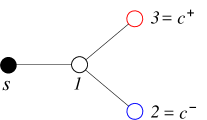
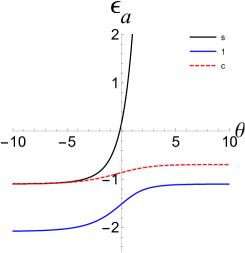
Figure 8: [Top] TBA diagram for $\lambda=\frac{1}{3}$. The black node is ”massive” (i.e. the associated QP, namely the soliton, carries energy) whereas empty nodes are associated to strings. [Bottom] QP spectrum for $\lambda=\frac{1}{3}$: the pseudo-energies $\epsilon_{a}(\theta)$ as a function of $\theta$, for $a\in\{s,1,c\}$, obtained by numerical integration of the TBA equations (48) at $V=0$.

Numerical integration of the TBA equations (48) at fixed $\frac{{\overline{V}}}{{\overline{T}}}$ yields the pseudo-energies $\epsilon_{a}(\frac{{\overline{V}}}{{\overline{T}}};\theta)$ that are displayed for $\frac{{\overline{V}}}{{\overline{T}}}=0$ in Fig. 8.(b).

VII.1.2 $\lambda=\frac{6}{19}$

The continued fraction decomposition $\lambda=\frac{1}{3+\frac{1}{6}}$ has $\alpha=2$ terms $\nu_{1}=3$, $\nu_{2}=6$, so from the numbers (Eq. (5)) $m_{1}=3$, $m_{\alpha}=9$ we see that we have $10=m_{\alpha}+1$ QPs, grouped in two families ${\cal F}_{1}=\{{A}_{s},{A}_{1},{A}_{2}\}$, ${\cal F}_{2}=\{{A}_{3},...,{A}_{7},{A}_{c}^{-}={A}_{8},{A}_{c}^{+}={A}_{9}\}$:     $\bullet$ the soliton ${A}_{s}$, carries energy and entropy, $\bullet$ the two charged strings ${A}_{c}^{\pm}$ carry entropy and charge $\pm{\mathfrak{q}}=\pm 19$, $\bullet$ all the other strings ${A}_{a=1,...,7}$ carry entropy only. The TBA diagram encoding the kernel is shown in Fig. 9.(a). The non-vanishing chemical potentials are $\mu_{c}^{\pm}=\pm\frac{19\overline{V}}{2\overline{T}}$. There are $m_{\alpha}=9$ independent pseudo-energies $\epsilon_{s}$, $\epsilon_{1,...,7}$ and $\epsilon_{c}$. The kernel has nearest neighbours entries involving two independent functions $\overline{\Phi}_{1}=\frac{1}{2\pi}\Phi^{\vphantom{\dagger}}_{p_{i}}$ with with $p_{1}=1$, $p_{2}=\frac{1}{6}$:

$$\overline{\Phi}^{\vphantom{\dagger}}_{1}(\theta)=\frac{1}{2\pi}\frac{1}{\cosh\theta}\qquad;\qquad\overline{\Phi}^{\vphantom{\dagger}}_{2}(\theta)=\frac{1}{2\pi}\frac{3}{\cosh 3\theta}$$

as well as a self-interaction entry involving the function $\frac{1}{2\pi}{\rm TF}^{-1}\big{[}\frac{\hat{\Phi}^{\vphantom{\dagger}}_{1}\hat{\Phi}^{\vphantom{\dagger}}_{1/6}}{\hat{\Phi}^{\vphantom{\dagger}}_{5/6}}\big{]}$:

$$\overline{\Phi}^{\vphantom{\dagger}}{}^{\mbox{\scriptsize self}}_{1,2}(\theta)=\frac{1}{4\pi}\int_{-\infty}^{\infty}d\omega\,e^{i\omega\theta}\,\frac{\cosh\frac{5\pi\omega}{12}}{\cosh\frac{\pi\omega}{2}\cosh\frac{\pi\omega}{12}.}$$

(a)    

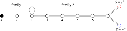
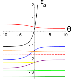
Figure 9: [Top] TBA diagram for $\lambda=\frac{6}{19}$. The black node is ”massive” (i.e. the associated QP, namely the soliton, carries energy) whereas empty nodes are associated to strings. [Bottom] QP spectrum for $\lambda=\frac{6}{19}$: the pseudo-energies $\epsilon_{a}(\theta)$ as a function of $\theta$, for $a\in\{s,1,2...,7,c\}$, obtaned by numerical integration of the TBA equations (51) at $V=0$. Compare the additional complexity in the spectrum with respect to the close value $\lambda=\frac{1}{3}$ in Fig. 8. Compare also the scales, in particular for the flatness of the last band (charged QPs ${A}_{c}^{\pm}$) when the denominator ${\mathfrak{q}}$ increases.

The signs of the two families are $\eta_{1}=$ and $\eta_{2}=-1$. The finite $V,T$ dimensionless densities $P_{a},\rho_{a}$ are determined by the TBA equations (6) which become:

$$\epsilon_{s} = e^{\theta}-\overline{\Phi}^{\vphantom{\dagger}}_{1}\star L_{1}$$

$$\epsilon_{1} = -\overline{\Phi}^{\vphantom{\dagger}}_{1}\star\big{(}L_{s}+L_{2}\big{)}$$

$$\epsilon_{2} = -\overline{\Phi}^{\vphantom{\dagger}}_{1}\star L_{1}-\overline{\Phi}^{\vphantom{\dagger}}{}^{\mbox{\scriptsize self}}_{1,2}\star L_{2}-\overline{\Phi}^{\vphantom{\dagger}}_{2}\star L_{3}$$

$$\epsilon_{3} = -\overline{\Phi}^{\vphantom{\dagger}}_{2}\star\big{(}-L_{2}+L_{4}\big{)}$$

$$\epsilon_{a} = -\overline{\Phi}^{\vphantom{\dagger}}_{2}\star\big{(}L_{a-1}+L_{a+1}\big{)}\qquad a=4,5,6$$

$$\epsilon_{7} = -\overline{\Phi}^{\vphantom{\dagger}}_{2}\star\big{(}L_{6}+L_{c^{+}}+L_{c^{-}}\big{)}$$

$$\epsilon_{c} = -\overline{\Phi}^{\vphantom{\dagger}}_{2}\star L_{7}$$ (51)

The denominator ${\mathfrak{p}}=6$ of $\lambda$ fixes the form of the transmission probability:

$${\cal T}_{\frac{6}{19}}(\theta)=\frac{1}{1+\big{(}{\overline{T}}e^{\theta}\big{)}^{-12}}$$ (52)

so the reduced current $\overline{I}=\frac{h}{ek_{\textsc{b}}T}I$ reads:

$$\overline{I}_{\!\frac{6}{19}}^{\vphantom{\dagger}}({\overline{V}},{\overline{T}})=19\!\int_{-\infty}^{\infty}\!\!\!d\theta\;{\cal T}_{\!\frac{6}{19}}(\theta)\;\frac{\partial}{\partial\theta}\ln\frac{1+e^{-\epsilon_{c}(\theta)-\frac{19\overline{V}}{2\overline{T}}}}{1+e^{-\epsilon_{c}(\theta)+\frac{19\overline{V}}{2\overline{T}}}}$$ (53)

Numerical integration of the TBA equations (51) at fixed $\frac{\overline{V}}{\overline{T}}$ yields the pseudo-energies $\epsilon_{a}(\frac{\overline{V}}{\overline{T}};\theta)$ that are displayed for $\frac{\overline{V}}{\overline{T}}=0$ in Fig. 9.(b).

VII.2 Bethe equations for solitons and strings

In this Appendix one gathers some technical details about the Algebraic Bethe Anstatz (ABA). One first starts (section VII.2.1) by presenting the discrete ABA equations constraining the allowed configurations $\mathscr{C}$ of QPs in terms of bare strings $B_{k_{j}}(\theta)$ (defined in Eq.(22)), and their continuum limit when the number of QPs goes to infinity. We then describe the dressing operation in section VII.2.2, implementing a transformation on the ensemble of solitons ${A}_{s}(\theta)$ and “bare” strings $B_{k_{j}}(\theta)$ to reproduce (a variant of) the quantization equations for solitons and strings first derived (for the string sector only) by Takahashi Takahashi72 ; TakahashiBook . Finally the effect of dressing on the charge is presented in section VII.2.3.

VII.2.1 Bare BA equations

We consider a configuration $\mathscr{C}$ comprising $N=N_{s}$ solitons at rapidities $\{\theta^{(s)}_{i}\}$ $(i=1,...,N_{s})$ and $N_{j}$ occupied strings of type $j$ at rapidities $\{\theta^{(j)}_{i}\}$ $(i=1,...,N_{j})$: $\mathscr{C}=\{\{\theta^{(s)}_{1},...,\theta^{(s)}_{N_{s}}\},\{\theta^{(1)}_{1},...,\theta^{(1)}_{N^{(1)}}\},...,\{\theta^{({m_{\alpha}})}_{1},...,\theta^{({m_{\alpha}})}_{N_{{m_{\alpha}}}}\}\}$. The requirement that the system be left invariant when an arbitrary particle is moved through all other particles and brought back to its initial position, for a system of finite length $L$, leads to the fundamental equations that define an allowed configuration:

$$e^{2i\pi{\cal N}_{s}(\theta)} = \tau^{(s)}_{\mathscr{C}}(\theta)\,e^{i\pi\delta_{s}}\,e^{-iLE_{0}\,e^{\theta}}$$

$$e^{2i\pi{\cal N}_{j}(\theta)} = \tau^{(j)}_{\mathscr{C}}(\theta)\,e^{i\pi\delta_{j}}\quad(j=1,...,{m_{\alpha}})$$ (54)

where the function ${\cal N}_{a}(\theta)$ evaluates to integers when $\theta=\theta^{(a)}_{i}$ is an occupied rapidity for species $a=s,1,...,{m_{\alpha}}$ (i.e. $\theta^{(a)}_{i}\in\mathscr{C}$), $\delta_{a}\in\{0,1\}$ is a constant (depending on $\mathscr{C}$) that will not be needed here, and where, in addition to the transfer matrix for solitons $\tau^{(s)}(\theta)$, one has introduced the transfer matrices for strings $\tau^{(j)}(\theta)$:

$$\tau_{\mathscr{C}}^{(j)}(\theta)=\prod_{i=1}^{N_{s}}S_{j,s}(\theta^{(s)}_{i}-\theta)\prod_{j^{\prime}=1}^{{m_{\alpha}}}\prod_{i=1}^{N_{j^{\prime}}}S_{j,j^{\prime}}(\theta^{(j^{\prime})}_{i}-\theta),$$ (55)

the scattering matrices being given in Eqs. (26,27). Note the presence of the factor $e^{ipL}$ in Eqs.(54) for solitons only, showing that the strings are fictitious particles carrying no momentum and no kinetic energy. The set of rapidities for which the right-hand side of Eqs.(54) evaluates to one is actually larger than $\mathscr{C}$: this defines additional, empty states called holes, at rapidities $\mathscr{C}^{h}=\{\theta^{(a),h}_{i}\}$. Thus, the total set of allowed rapidities (or “Bethe roots”) is $\mathscr{C}\cup\mathscr{C}^{h}$.

Introducing the (reduced) total density of Bethe roots per unit length, $P_{a}=-\eta_{a}\,(-1)^{\delta_{a,s}+\delta_{a,{m_{\alpha}}}}\,\frac{1}{E_{0}L}\frac{d{\cal N}_{a}}{d\theta}$ (the signs $\eta_{a}$ are necessary to obtain a positive densityTakahashi72 ) as well as the (reduced) density of occupied Bethe roots per unit length $\tilde{\rho}_{a}$, and taking the derivative of the logarithm of Eqs.(54) yields in the thermodynamical limit $L\to\infty$:

$$-\eta_{a}\,(-1)^{\delta_{a,s}+\delta_{a,{m_{\alpha}}}}\,P_{a}=\delta_{a,s}e^{\theta}+\frac{1}{2\pi}\Phi_{a,b}\star\tilde{\rho}_{b}$$ (56)

with $\Phi_{ab}(\theta)=-i\partial_{\theta}\log S_{ab}(\theta)$ and the scattering matrix elements are given in Eqs. (26,27). Since all particles scatter non-trivially on all others, the bare kernel $\Phi_{ab}(\theta)$ has a complicated structure. It can be made explicit in Fourier space using the elementary function $\hat{\varphi}_{k}^{(\varepsilon)}(\omega)=\frac{1}{2i\pi}\int d\theta e^{-i\omega\theta}\partial_{\theta}\log g^{(\varepsilon)}_{k}(\theta)$ (the function $g_{k}^{(\varepsilon)}$ is defined in (28)), that reads

$$\hat{\varphi}_{k}^{(+)}(\omega) = (1-\delta_{\tilde{k},0})\;\;\frac{\sinh((1-\tilde{k}\lambda)\frac{\pi\omega}{2\lambda})}{\sinh(\frac{\pi\omega}{2\lambda})}$$ (57)

$$\hat{\varphi}_{k}^{(-)}(\omega) = \hat{\varphi}_{k+\lambda^{-1}}^{(+)}(\omega)$$

where $\tilde{k}=\frac{2}{\lambda}\big{]}\frac{k\lambda}{2}\big{[}$ and $]x[=x-[x]$ is the fractional part of $x$.

VII.2.2 Dressed BA equations

It is very convenient, to simplify the continuous Bethe equations (56), to perform a particle-hole transformation by defining $\rho_{j}=\rho_{j}^{(-)}$ (and $\tilde{\rho}^{(+)}=P_{j}-\rho_{j}$) on all strings of type $j<{m_{\alpha}}$. It means that we describe an allowed, but empty Bethe root $\theta^{(j)}_{i}\in\mathscr{C}^{h}$ – i.e. $\theta^{(j)}_{i}$ is solution of the Bethe equation $\tau^{(j)}(\theta^{(j)}_{r})=e^{i\pi\delta_{j}}$, but there is no insertion of the corresponding operator $B_{k_{j}}(\theta^{(j)}_{r})$ in the product (20) – as an occupied state for a new particle ${A}_{j}(\theta)$ at $\theta=\theta^{(j)}_{i})$, whereas an initially occupied $B_{k_{j}}(\theta^{(j)}_{i})$ string is described as an allowed but empty ${A}_{j}(\theta^{(j)}_{i})$ state. Thus the new particles ${A}_{j}$ are holes in an (interacting) sea of strings. This sea could be termed the Zamalodchikov-Fateev sea ; it is the new vacuum, and formally reads:

$$\left|0\right\rangle_{\rm dr}=\prod_{j=1}^{{m_{\alpha}}-1}\;\;\prod_{\theta^{(j)}_{i}\in\mathscr{C}\cup\mathscr{C}^{h}}B_{k_{j}}(\theta^{(j)}_{i})\;\;|\Omega\rangle.$$ (58)

We also introduce ${A}_{{m_{\alpha}}}(\theta)=B_{k_{{m_{\alpha}}}}(\theta)$, with density $\rho_{{m_{\alpha}}}=\tilde{\rho}_{{m_{\alpha}}}$, and define $\rho_{s}=\tilde{\rho}_{s}$ since the soliton mode is unaffected by dressing. The new reference state $(\ref{defZFS})$, is a highly interacting object, causing the excitations ${A}_{j}(\theta)\left|0\right\rangle_{\rm dr}$ above it to be dressed by their interaction with the sea. This dressing affects both the scattering and the charge densities.

The effect of the particle-hole transformation is described by introducing the projector $\mathbb{P}$ onto strings that are affected by the particle-hole transformation (i.e. $\mathbb{P}_{ab}=\delta_{ab}(1-\delta_{a,{m_{\alpha}}}-\delta_{as})$), the diagonal matrix ${\bm{\eta}}$ with entries $\eta_{j,j^{\prime}}=\delta_{j,j^{\prime}}\eta_{j}^{\vphantom{\dagger}}$, the vector $\hat{\bm{P}}$ in Fourier space with components $\hat{P}_{j}$, the bare kernel $\hat{\bm{\Phi}}$ with components $\hat{\Phi}_{j,j^{\prime}}$, and the vector $\hat{\bm{\Phi}}^{(s)}$ with components $\hat{\Phi}_{s,j}$. Using $\tilde{\bm{\rho}}^{(+)}=\mathbb{P}{\bm{P}}+(1-2\mathbb{P}){\bm{\rho}}$, we have from (56): $-{\bm{\eta}}\hat{\bm{P}}=\hat{\bm{\Phi}}\Big{(}\mathbb{P}\hat{\bm{P}}+(1-2\mathbb{P})\hat{\bm{\rho}}\Big{)}+\hat{\bm{\Phi}}^{(s)}\hat{\rho}_{s}$ which can be recast as $\hat{\bm{P}}=\hat{\bm{K}}\hat{\bm{\rho}}+\hat{\bm{K}}^{(s)}\hat{\rho}_{s}$, defining the dressed string-string kernel $\hat{\bm{K}}=({\bm{\eta}}+\hat{\bm{\Phi}}\mathbb{P})^{-1}\hat{\bm{\Phi}}(2\mathbb{P}-1)$ and the dressed string-soliton kernel $\hat{\bm{K}}^{(s)}=-({\bm{\eta}}+\hat{\bm{\Phi}}\mathbb{P})^{-1}\hat{\bm{\Phi}}^{(s)}$. We have checked explicitly that the resulting dressed kernel for the QPs ${A}_{a}(\theta)$ has the minimal simple structure given in Fig. 4), leading to the continuous dressed BA equations Eq. (30). The dressed kernel $K$ is non symmetric but rather $K_{ba}=\eta_{a}\eta_{b}K_{ab}$.

VII.2.3 Charge dressing

Here we discuss how the charge of the QPs is affected by dressing. The presentation (30) of the BA equations is very close to that initially obtained by Takahashi Takahashi72 ; TakahashiBook with the difference of the explicitation of the ZF-sea (58) (the dressed vacuum). After the particle-hole transformation it is not so clear a priori how we should, if we can, attach definite charges to the new QPs: indeed, they are holes in a filled interacting ZF-sea, and the structure of this filled sea itself (depth, density of states, etc…) depends on the whole configuration ; we furthermore expect a non-trivial effect of the scattering of the new QPs ${A}_{j}$ on the (configuration-dependent) background seas. This question is answered by considering the charge density whose Fourier transform can be expressed at the bare level as $\hat{\rho}_{Q}=\sum_{a=s,1,...,{m_{\alpha}}}\tilde{Q}_{a}\widehat{\tilde{\rho}}^{(+)}_{a}$ where $\tilde{\rho}_{a}^{(+)}$ are the bare densities entering (56), with the bare components of the charge vector reading $\tilde{Q}_{s}=-1$ (the state $\left|\Omega\right\rangle$ is filled with antisolitons) and $\tilde{Q}_{j}=+2k_{j}$ with $k_{j}$ given by Eq. (23) (since the string $B_{k_{j}}$ consists in $k_{j}$ magnons each contributing twice the elementary soliton charge). We then get the dressed charge vector $Q_{a}$ defining the charge in the dressed basis as (we use $K_{ba}=\eta_{a}\eta_{b}K_{ab}$):

$$\rho_{Q}(\theta) = \frac{1}{2\pi}(Q_{a}\star\rho_{a})(\theta)$$ (59)

$$\hat{\bm{Q}}(\omega) = (\bm{\eta K}(\omega){\bm{\eta}}\mathbb{P}+1-2\mathbb{P})\tilde{\bm{Q}}$$ (60)

Observe in Eq. (59) how the convolution with the function $Q_{a}(\theta)$ describes a spreading of the charge due to scattering of the dressed QPs with the ZF-sea: writing $\hat{Q}_{a}(\omega)=2\pi\delta(\theta)\hat{Q}_{a}(0)+(\hat{Q}_{a}(\theta)-2\pi\delta(\theta)\hat{Q}_{a}(0))$ the second term shows that indeed charge is not local in rapidity space. But due to the sort-range nature of the matrix elements of $K_{ab}(\theta)$ (they all have exponential decay), for quantities that are obtained by integration over a sizeable ($\gg 1$) $\theta-$range one can replace $K_{ab}(\theta)\to(\int K_{ab})\delta(\theta)$. In particular when doing thermodynamics in the grand canonical ensemble one only needs the total charge of the configuration $Q_{\mathscr{C}}^{\vphantom{\dagger}}=^{\vphantom{\dagger}}\int_{-\infty}^{\infty}d\theta\;\rho_{Q}(\theta)$ so the aforementionned spreading is washed out by $\theta-$averaging. We check explicitly that

$$\hat{\bm{Q}}(\omega)\underset{\omega\to 0}{\longrightarrow}(0,...,0,-{\mathfrak{q}},{\mathfrak{q}})$$ (61)

with ${\mathfrak{q}}$ the denominator of $\lambda$ so that finally:

$$Q_{\mathscr{C}}^{\vphantom{\dagger}}={\mathfrak{q}}\;\Big{(}N_{{m_{\alpha}}}-N_{{m_{\alpha}}-1}\Big{)}={\mathfrak{q}}\Big{(}N_{c}^{+}-N_{c}^{-}\Big{)},$$ (62)

establishing that effectively all QPs are neutral except for the last two strings carry charge $\pm{\mathfrak{q}}$, and motivating the introduction of the final notation ${A}_{c}^{+}\equiv{A}_{{m_{\alpha}}}$ and ${A}_{c}^{-}\equiv{A}_{{m_{\alpha}}-1}$ for the last two QPs. This readily fixes the chemical potentials $\mu_{a}=\frac{{\mathfrak{q}}V}{2T}(\delta_{a,c^{+}}-\delta_{a,c^{-}})$ for the description of the finite bias $V$ situation.

VII.2.4 Alternative dressing

In this section one gives a last change of basis (an alternative kind of dressing) leading to yet another presentation of the TBA equations sometimes used in the literature. It can be obtained, starting from the dressed basis used in the main text, by performing a particle-hole transformation on those dressed QPs having $\eta_{j}=-1$. It leads to a modified dressed vacuum, and affects the scattering in a way that we will shortly describe, as well as the charge that now reads: $Q=\eta_{\alpha}{\mathfrak{q}}(\tilde{N}_{{m_{\alpha}}}-\tilde{N}_{{{m_{\alpha}}}-1})$: the QPs $A_{{m_{\alpha}}}$ now has charge $\eta_{\alpha}{\mathfrak{q}}$. Defining $\tilde{\epsilon}_{a}=\eta_{a}\epsilon_{a}$, $\tilde{L}^{(\pm)}_{a}=\ln(1+e^{\pm\big{(}\mu_{a}-\epsilon_{a})}\big{)}$, as well as the densities $\tilde{\rho}_{a}^{(\pm)}$ of occupied and empty QP states as $\tilde{\rho}_{a}^{(\pm)}=\rho_{a}$ if $\eta_{a}=\pm 1$, $\tilde{\rho}_{a}^{(\pm)}=P_{a}-\rho_{a}$ if $\eta_{a}=\mp 1$. This leads to a new presentation of the BA equations (30) and of the TBA equations (6):

$$P_{a} = \delta_{as}\,e^{\theta}+\frac{1}{2\pi}\big{(}\tilde{K}_{ab}\star\tilde{\rho}^{(\eta_{b})}\big{)}(\theta)$$

$$\tilde{\epsilon}_{a} = \delta_{as}e^{\theta}-\frac{1}{2\pi}\big{(}\tilde{K}_{ab}\star\tilde{L}^{(\eta_{b})}\big{)}(\theta)$$ (63)

The new BA/TBA system has a symmetric dressed Kernel $\tilde{K}_{ab}=-\eta_{a}K_{ab}$, this nevertherless comes with the price that the BA/TBA system has a less homogeneous form since it now involves explicitly the signs $\eta_{a}$. This has the physical meaning, that when a QP $a$ goes through the gas of other QPs, it accumulates a phase-shift that is determined by the particles $b$ it crosses when $\eta_{b}=1$, or by the holes it crosses when $\eta_{b}=-1$.

VII.3 Asymptotics of the TBA equations

In this Appendix one gives the explicit form of the asymptotics of the pseudo energies $\epsilon_{a}(\theta)$ in the limits $\theta\to+\infty$ (UV limit) and $\theta\to-\infty$ (IR limit), starting from the TBA equations (6). It is convenient to work with the quantities $X_{a}=e^{-\epsilon_{a}(+\infty)}$ and $Y_{a}=e^{-\epsilon_{a}(-\infty)}$ (one also defines $X_{c}\equiv X_{{m_{\alpha}}-1}=X_{{m_{\alpha}}}$, $X_{0}\equiv X_{s}$, and $Y_{c}\equiv Y_{{m_{\alpha}}-1}=Y_{{m_{\alpha}}}$, $Y_{0}\equiv Y_{s}$). The analysis in the diagonal case can be found e.g. in Ref. Klassen90 and we give here its off-diagonal generalization.

In the UV limit, the source term $\delta_{as}e^{\theta}$ in (6) dominates and fixes the behavior $\epsilon_{s}(\theta)\sim e^{\theta}$, implying $X_{s}=0$. On the other hand, the string pseudo-energies have finite limits. Using $\frac{1}{2\pi}\int_{\mathbb{R}}d\theta K_{ij}(\theta)=\frac{1}{2}I_{ij}$ where $I_{ij}$ is the (signed) incidence matrix of the TBA diagram (see Fig. 4) yields ${m_{\alpha}}-1$ coupled equations for the quantities $X_{a}\big{(}\lambda,\frac{V}{T}\big{)}$:

$$\begin{array}[]{rll}&&a\notin\{m_{i}-1,m_{i},{m_{\alpha}}-2,c\}:\\ X_{a}^{2}&=&(1+X_{a-1})(1+X_{a+1})\\ &&i<\alpha:\\ X_{m_{i}-1}^{2}&=&(1\!+\!X_{m_{i}-2})(1\!\!+\!\!X_{m_{i}-1})(1+X_{m_{i}}),\\ X_{m_{i}}^{2}&=&\frac{1+X_{m_{i}+1}}{1+X_{m_{i}-1}},\\ X^{2}_{{m_{\alpha}}-2}&=&(1\!\!+\!\!X_{{m_{\alpha}}-3})(1\!\!+\!\!X_{c}e^{{\mathfrak{q}}V/2T})(1\!\!+\!\!X_{c}e^{-{\mathfrak{q}}V/2T})\\ X_{c}^{2}&=&1+X_{{m_{\alpha}}-2}\end{array}$$ (64)

The solution is found to be

$$X_{s} = 0$$

$$(a\neq s,c)\qquad\quad X_{a} = \Big{(}\frac{\sinh((y_{\mathfrak{i}(a)-1}+k_{a})\frac{V}{2T})}{\sinh(y_{\mathfrak{i}(a)-1}\frac{V}{2T})}\Big{)}^{2}-1$$

$$X_{c} = \frac{\sinh(({\mathfrak{q}}-y_{\alpha-1})\frac{V}{2T})}{\sinh(y_{\alpha-1}\frac{V}{2T})}$$ (65)

where the integer $\mathfrak{i}(a)$ is defined by the fact that QP $a$ belongs to the family ${\cal F}_{\mathfrak{i}(a)}$.

In the IR limit $\theta\to-\infty$, the source term $\delta_{as}e^{\theta}$ in the TBA equations (6) vanishes and the $``s"$ node behaves as if it where a massless node added to the family ${\cal F}_{1}$. All pseudo-energies have finite limit and one readily obtains

$$\{Y_{s},Y_{1}...Y_{{m_{\alpha}}-2},Y_{c}\}=\{\tilde{X}_{1},\tilde{X}_{2}...\tilde{X}_{{m_{\alpha}}-1},\tilde{X}_{c}\}$$ (66)

where $\tilde{X}_{a}=X_{a}\big{(}\tilde{\lambda},\frac{{\mathfrak{q}}}{\tilde{\mathfrak{q}}}\frac{V}{T}\big{)}$ and $\tilde{\lambda}=\frac{\lambda}{\lambda+1}=\frac{\tilde{\mathfrak{p}}}{\tilde{\mathfrak{q}}}$ is the rational number with continued fraction $\{\nu_{1}+1,\nu_{2},..,\nu_{\alpha}\}$.

VII.4 Bulk thermodynamical quantities

In this Appendix we present the expressions of the thermodynamical quantities for the gas of interacting dressed QPs ${A}_{a}(\theta)$.

VII.4.1 Free energy

As a fundamental check of the consistency of the approach, one can compare the free energy of the interacting QP gas at finite $(V,T)$, to that of a free boson under the same conditions – the massless limit of the SG model being indeed a very complicated representation of a free massless boson.

Writing the free energy of the bulk massless SG model as $F=\frac{LT^{2}}{2\pi}\bar{F}$, one decomposes the free energy as $\bar{F}=\bar{E}-T\bar{S}-\sum_{a}\mu_{a}\bar{N}_{a}$ with the reduced energy $\bar{E}=\int d\theta\,\rho_{s}(\theta)\,e^{\theta}$ (remember that only the soliton carries energy), the particle numbers $\bar{N}_{a}=\int d\theta\rho_{a}(\theta)$ and the entropy $-T\bar{S}=\int d\theta P_{a}(\theta)\left[f_{a}(\theta)\ln f_{a}(\theta)+(1-f_{a}(\theta))\ln(1-f_{a}(\theta))\right]$. After a few manipulations it can be recast as:

$$\bar{F}=\bar{E}-\widetilde{\bar{E}}-\sum_{a}\int d\theta\,P_{a}L_{a}$$ (67)

where the last term can be expressed as an ordinary definite integral on the variables $\epsilon_{a}$ using $P_{a}=\eta_{a}\partial_{\theta}\epsilon_{a}$ and one has introduced the (reduced) “total pseudo energy” of the system $\widetilde{\bar{E}}=\sum_{a}\int d\theta\,\rho_{a}(\theta)\,\epsilon_{a}(\theta)$.

Using a remarkable trick FreeEnergyCalc , the difference $\bar{E}-\widetilde{\bar{E}}$ can be expressed in a closed form involving only the limiting values $\epsilon_{a}(\pm\infty)$: $\bar{E}-\widetilde{\bar{E}}=\int\rho_{a}(K_{ba}\star L_{b})=-\eta_{a}\int L_{a}^{\prime}(K_{ba}\star L_{b})=-\eta_{a}[L_{a}(K_{ba}\star L_{b})]_{-\infty}^{\infty}+\eta_{a}\int L_{a}(K_{ba}\star L_{b}^{\prime})$ where the last term of this last form can be shown to be nothing but $-(\bar{E}-\widetilde{\bar{E}})$ using $\int f(g\star h)=\int h(g\star f)$ valid for arbitrary functions $f,h$ and any even function $g$. Finally we obtain $\bar{E}-\widetilde{\bar{E}}=-\frac{1}{2}\eta_{a}[L_{a}(K_{ba}\star L_{b})]_{-\infty}^{+\infty}$.

Collecting all terms one ends up with the following explicit expression for the free energy per unit length:

$$\frac{F(V,T)}{L}=\frac{T^{2}}{2\pi}\;\!\!\sum_{a=s,1,...,{m_{\alpha}}}\!\!\!\!\eta_{a}\Big{[}{\cal F}_{\mu_{a}}(x)\Big{]}_{x=X_{a}}^{x=Y_{a}},$$ (68)

where the function ${\cal F}_{\mu}$ is given by

$${\cal F}_{\mu}(x)=\mbox{Li}_{2}\big{(}-xe^{\mu}\big{)}+\frac{1}{2}\ln(x)\ln(1+xe^{\mu}).$$ (69)

Here $\mbox{Li}_{2}(x)=-\int_{0}^{x}\frac{dt}{t}\,\ln(1-t)$ is the second polylogarithm function and $(X_{a},Y_{a})$ are respectively the UV and IR limits of $e^{-\tilde{\epsilon}_{a}}$ given in (65) and (66), and one reminds that the chemical potential are given by $\mu_{a}=\frac{{\mathfrak{q}}V}{2T}(\delta_{a,c^{+}}-\delta_{a,c^{-}})=\frac{{\mathfrak{q}}V}{2T}(\delta_{a,{m_{\alpha}}}-\delta_{a,{m_{\alpha}}-1})$.

The interacting QP gas should be equivalent at the level of the free energy to a free massless boson with Hamiltonian $H_{\mbox{\scriptsize free}}=\int_{0}^{L}\left[(\partial_{x}\phi(x))^{2}-\frac{V}{2}Q(x)\right]$ and periodic boundary conditions, or

$$H_{\mbox{\scriptsize free}}=\int_{0}^{L}\big{[}(\partial_{x}\phi(x))^{2}-\frac{V}{\sqrt{2\pi(\lambda+1)}}\,\partial_{x}\phi(x)\big{]}$$ (70)

where one has used the normalization (3) of the charge. The computation of the free energy is standard and one finds (see e.g. BookDifrancesco ):

$$\frac{F_{{\mbox{\scriptsize free}}}}{L}=-\frac{T^{2}}{2\pi}\bigg{(}\frac{\pi^{2}}{6}+\frac{1}{\lambda+1}\Big{(}\frac{V}{2T}\Big{)}^{2}\bigg{)}.$$ (71)

It is not obvious that the expressions (68) and (71) do actually coincide for all $\lambda$. We checked that it is indeed the case with numerical accuracy $\sim 10^{-15}$ and for all rational $\lambda$’s with lengths $m_{\alpha}$ up to 15: this expresses the equivalence of the partition functions of the free bose gas and of the interacting QP gas (thanks to a infinity of polylogarithm identities).

VII.4.2 Entropy

The entropy carried by each particle can be computed directly using the same arguments. For species $a=s,1,...,{m_{\alpha}}$, defining the dimensionless entropy $\overline{S}_{a}=\frac{hv_{\textsc{f}}}{Lk_{\textsc{b}}^{2}T}S_{1}$, one finds:

$$\overline{S}_{a}=-\eta_{a}\Big{[}2{\cal F}_{\mu_{a}}(x)+\mu_{a}\ln(1+xe^{\mu_{a}})\Big{]}_{X_{a}}^{Y_{a}}$$ (72)

In the large voltage limit, using (65, 66) we get that for all $a\neq s$, $X_{a}$ and $Y_{a}$ are exponentially large. Using the limit ${\cal F}_{0}(x)\underset{x\to\infty}{\longrightarrow}-\frac{\pi^{2}}{6}$, we conclude immediately that $S_{a}\longrightarrow 0$. Taken care of the additional chemical potential term, we also get $S_{c}\to 0$: this expresses the freezing of the string entropies in the limit $V/T\to 0$. In the means time the solitons carry all the entropy $\overline{S}_{s}=\frac{\pi^{2}}{3}$ that coincides with the (voltage independent) entropy of the original free thermal boson.

On the other hand, in the low voltage limit, strings do carry a finite entropy. The part of the entropy carried by the solitons can be estimated using (65, 66) : we have $X_{s}=0$ and $Y_{s}=3$. Note that these limiting values are independent of $\lambda$. Plugging those values into (72), using that $\sum_{a}\overline{S}_{a}=\frac{\pi^{2}}{3}$ and after a little algebra, we get the universal formula (31).

VII.4.3 Particle number

The reduced particle number for species $a$, $\overline{N}_{a}=\frac{2\pi}{LT}\big{\langle}\hat{N}_{a}\big{\rangle}_{V,T}=\int d\theta\rho_{a}(\theta)$, can be easily related to the asymptotic values $X_{a},Y_{a}$ Eqs. (65,66) of the function $e^{\epsilon_{a}(\theta)}$ at $\theta=\pm\infty$. Since $\rho_{a}=-\eta_{a}\partial_{\theta}L_{a}(\theta)$ we get

$$\overline{N}_{a}\Big{(}\lambda;\frac{{\overline{V}}}{{\overline{T}}}\,\Big{)}=\eta_{a}\ln\bigg{(}\frac{1+Y_{a}e^{\mu_{a}}}{1+X_{a}e^{\mu_{a}}}\bigg{)}.$$ (73)

VII.4.4 Average charge

The average charge accumulated in the system at finite $(V,T)$ can be of course obtained by differentiating the free energy (68) with respect to $V$. But it can also more directly be computed by just counting (${\mathfrak{q}}$ times) the difference in the occupation number of charged QPs $\overline{Q}\equiv\frac{2\pi}{LT}\langle\hat{Q}\rangle_{V,T}={\mathfrak{q}}\int d\theta(\rho_{c}^{+}-\rho_{c}^{+})$. Using $\rho_{c}^{\pm}=-\eta_{\alpha}\partial_{\theta}^{\vphantom{\dagger}}L_{c}^{\pm}$ one arrives at:

$$\overline{Q} = {\mathfrak{q}}\,\eta_{\alpha}\Bigg{[}\ln\bigg{(}\frac{1+Y_{c}e^{\frac{{\mathfrak{q}}V}{2T}}}{1+X_{c}e^{\frac{{\mathfrak{q}}V}{2T}}}\bigg{)}-\;\ln\bigg{(}\frac{1+Y_{c}e^{-\frac{{\mathfrak{q}}V}{2T}}}{1+X_{c}e^{-\frac{{\mathfrak{q}}V}{2T}}}\bigg{)}\Bigg{]}$$ (74)

$$= \frac{1}{\lambda+1}\;\frac{V}{T}$$

where the last equality uses (65,66). This is of course consistent with a direct calculation within the free boson model (70).

VII.5 Some properties of the continued fraction decomposition

In this Appendix one presents some basic useful elements about the continued fraction defining the rational SG parameter $\lambda<1$ (in the repulsive case)

$$\lambda=\frac{{\mathfrak{p}}}{{\mathfrak{q}}}=\frac{1}{\nu_{1}+\frac{1}{\nu_{2}+...\frac{1}{\nu_{\alpha}}}}\equiv\{\nu_{1},\nu_{2},...,\nu_{\alpha}\}.$$ (75)

The recursive nature of the continued fraction representation can be elucidated by associating to $\lambda$ the function $F_{\lambda}(x)$ defined by the continued fraction $F_{\lambda}(x)=\{\nu_{1},...,\nu_{\alpha},x\}=\frac{1}{\nu_{1}+\frac{1}{\nu_{2}+...+\frac{1}{\nu_{\alpha}+x}}}$. One has $F_{\lambda}(0)=\lambda$ and $F_{\lambda}(\infty)=\breve{\lambda}=\{\nu_{1},...,\nu_{\alpha-1}\}$. Of course this function can be obtained repeated applications of elementary functions $F_{\frac{1}{\nu}}(x)=\frac{1}{\nu+x}$, i.e. $F_{\lambda}(x)=F_{\frac{1}{\nu_{1}}}\circ...\circ F_{\frac{1}{\nu_{\alpha}}}(x)$.

A connexion with $GL(2,\mathbb{Z})$, the group of $2\times 2$ unimodular matrices, emerges if one associates to $F_{\lambda}$ a matrix $M_{\lambda}$ with positive integer coefficients such that $F_{\lambda}(x)=\frac{(M_{\lambda})_{11}x+(M_{\lambda})_{12}}{(M_{\lambda})_{21}x+(M_{\lambda})_{22}}$. For elementary functions $M_{\frac{1}{\nu}}=\Big{(}{\small\begin{array}[]{cc}0&1\\ 1&\nu\end{array}}\Big{)}$ and it is easy to check that the matrix associated to $\lambda$ is $M_{\lambda}=M_{\frac{1}{\nu_{1}}}M_{\frac{1}{\nu_{1}}}...M_{\frac{1}{\nu_{\alpha}}}$. The function $-F_{\lambda}(-x)$ is an element of the modular group, and the matrix $M_{\lambda}$ is an element of $GL(2,\mathbb{Z})$. Since $\mbox{Det}(M_{\frac{1}{\nu}})=-1$, one has immediately $\mbox{Det}(M_{\lambda})=(-1)^{\alpha}$. Furthermore, by looking at the definition of the integers $y_{i}$ (defined in Eq. (25)), one can express explicitly the function $F_{\lambda}$ (and hence the matrix $M_{\lambda}$) as $F_{\lambda}(x)=\frac{\breve{y}_{\alpha-2}x+\breve{y}_{\alpha-1}}{y_{\alpha-1}x+y_{\alpha}}$ or

$$F_{\lambda}(x)=\frac{{\mathfrak{p}}^{\prime}x+{\mathfrak{p}}}{{\mathfrak{q}}^{\prime}x+{\mathfrak{q}}}$$ (76)

where the last equality defines the integers ${\mathfrak{p}}^{\prime}[\lambda]=\breve{y}_{\alpha-2}$ and ${\mathfrak{q}}^{\prime}[\lambda]=y_{\alpha-1}$. From this we deduce the relation

$${\mathfrak{p}}^{\prime}{\mathfrak{q}}-{\mathfrak{p}}\,{\mathfrak{q}}^{\prime}=(-1)^{\alpha}.$$ (77)

This gives a (not so practical) way to obtain the value of the integer ${\mathfrak{q}}^{\prime}[\lambda]=y_{\alpha-1}$ starting from the integers $({\mathfrak{p}},{\mathfrak{q}})$: it is (up to a sign $(-1)^{\alpha+1}$) the multiplicative inverse of ${\mathfrak{p}}$ in the cyclic group $\mathbb{Z}_{\mathfrak{q}}=\mathbb{Z}/({\mathfrak{q}}\mathbb{Z})$ (this inverse exists since ${\mathfrak{p}}\wedge{\mathfrak{q}}=1$), so that denoting by $\star_{{\mathfrak{q}}}$ the multiplication in $\mathbb{Z}_{\mathfrak{q}}$ one has ${\mathfrak{p}}\star_{{\mathfrak{q}}}{\mathfrak{q}}^{\prime}=(-1)^{\alpha+1}$.

VII.5.1 Scattering matrix for the pair of strings $B_{k_{{m_{\alpha}}}}(\theta)B_{k_{{m_{\alpha}}-1}}(\theta)$

Here we gives details about the representation of the U(1) charge symmetry at the level of bare ABA: the particle-hole operation exchanges the two last strings $B_{{m_{\alpha}}}$ and $B_{{m_{\alpha}}-1}$. We first check that the pair of strings $B_{k_{{m_{\alpha}}}}(\theta)B_{k_{{m_{\alpha}}-1}}(\theta)$ is transparent in the sense that

$$S_{a,{m_{\alpha}}}(\theta)S_{a,{m_{\alpha}}-1}(\theta)=1\quad\forall\,\theta,\quad\forall\,a=s,1,...,{m_{\alpha}}.$$ (78)

To see this, in view of Eq. (26), it is enough to show that $S_{1,{m_{\alpha}}}(\theta)S_{1,{m_{\alpha}}-1}(\theta)=1$ $\forall\theta$. Let us compute the parities: using (77) we get $\varepsilon_{{m_{\alpha}}}=(-1)^{{\mathfrak{p}}^{\prime}}e^{i\pi[((-1)^{\alpha+1}-{\mathfrak{p}})/{\mathfrak{q}}]}=(-1)^{{\mathfrak{p}}^{\prime}+1}$ (the exceptional case $\alpha=1$ has to be treated separately and yields the same result) and similarly $\varepsilon_{{m_{\alpha}}-1}=(-1)^{{\mathfrak{p}}+{\mathfrak{p}}^{\prime}+1}$ so that $\varepsilon_{{m_{\alpha}}}\varepsilon_{{m_{\alpha}}-1}=(-1)^{{\mathfrak{p}}}$. When ${\mathfrak{p}}$ is even, the strings have same parities and the imaginary shifts $\lambda k\frac{\pi}{2}$ in the functions $g_{k}$ are such that $\lambda(k_{{m_{\alpha}}}+k_{{m_{\alpha}}-1})$ is an even integer so that $S_{1,{m_{\alpha}}}S_{1,{m_{\alpha}}-1}=1$. On the other hand when ${\mathfrak{p}}$ is odd, the strings have opposite parities and the scattering matrix of the negative parity string is built on $g^{(-)}_{k}=g^{(+)}_{k+\lambda^{-1}}$ : the imaginary shifts are then such that $\lambda(k_{{m_{\alpha}}}+k_{{m_{\alpha}}-1})+1$ is again an even integer so that again $S_{1,{m_{\alpha}}}S_{1,{m_{\alpha}}-1}=1$.

An immediate consequence is that (see the definition of the transfer matrices for strings, Eqs. (55) in Appendix VII.2) the spectrum for the last two strings is degenerate, i.e. a given rapidity $\theta$ is an allowed rapidity for the last string $B_{k_{{m_{\alpha}}}}$ if and only if it is an allowed rapidity for the one-but-last string $B_{k_{{m_{\alpha}}-1}}$. This degeneracy is of course related to charge conjugation symmetry, and results in the last two pseudo-energies coinciding, $\epsilon_{c^{+}}=\epsilon_{c^{-}}$, in the continuous limit.

VII.5.2 Computation of $G_{0}\propto[f_{c}(\theta)]_{-\infty}^{+\infty}$, and $N_{c}^{\pm}\propto[L^{\pm}_{c}(\theta)]_{-\infty}^{+\infty}$

Here we compute the the quantity $\Delta f_{c}=f_{c}(+\infty)-f_{c}(-\infty)$ that determines the high temperature linear conductance. Taking the limit $V\to 0$ in Eqs. (65) and (66), one has $X_{c}=\frac{{\mathfrak{q}}-{\mathfrak{q}}^{\prime}}{{\mathfrak{q}}^{\prime}}$ and $Y_{c}=\frac{\tilde{\mathfrak{q}}-\tilde{\mathfrak{q}}^{\prime}}{\tilde{\mathfrak{q}}^{\prime}}$. From this we deduce $f_{c}(\infty)=\frac{1}{1+X_{c}^{-1}}=1-\frac{{\mathfrak{q}}^{\prime}}{{\mathfrak{q}}}$ and a similar expression for $f_{c}(-\infty)$ so that $\Delta f_{c}=\frac{\tilde{\mathfrak{q}}^{\prime}}{\tilde{\mathfrak{q}}}-\frac{{\mathfrak{q}}^{\prime}}{{\mathfrak{q}}}$. Since $\tilde{\lambda}=\frac{\lambda}{\lambda+1}$, we immediately have $\tilde{\mathfrak{q}}={\mathfrak{p}}+{\mathfrak{q}}$, while $\tilde{\mathfrak{q}}^{\prime}$ is determined by the relation ${\mathfrak{p}}\star_{{\mathfrak{p}}+{\mathfrak{q}}}\tilde{\mathfrak{q}}^{\prime}=(-1)^{\alpha+1}$: but this does not give an explicit value for $\tilde{\mathfrak{q}}^{\prime}$. To proceed, we consider the function $F_{\tilde{\lambda}}(x)$: one has $F_{\tilde{\lambda}}=\frac{1}{1+\frac{1}{F_{\lambda}}}=\frac{{\mathfrak{p}}^{\prime}x+{\mathfrak{p}}}{({\mathfrak{p}}^{\prime}+{\mathfrak{q}}^{\prime})x+{\mathfrak{p}}+{\mathfrak{q}}}$ showing that $\tilde{\mathfrak{q}}^{\prime}={\mathfrak{p}}^{\prime}+{\mathfrak{q}}^{\prime}$. After a little algebra we conclude that

$$\Delta f_{c}=\frac{(-1)^{\alpha}}{{\mathfrak{q}}^{2}(\lambda+1)}.$$ (79)

This yields the expected result for the linear conductance $G_{0}(T)=\partial_{V}I(V,T)\big{|}_{V=0}$

$$\frac{h}{e^{2}}G_{0}(\infty)=-\,\eta_{\alpha}\,{\mathfrak{q}}^{2}\Delta f_{c}=\frac{1}{\lambda+1},$$ (80)

which is indeed a continuous function of $\lambda$.

Using the same tricks one calculates the number of occupied charged strings per unit length, $\frac{2\pi}{LT}N_{c}^{\pm}=\bar{N}_{c}^{\pm}=\eta_{\alpha}\rho_{c}^{\pm}=-\eta_{\alpha}[\ln\big{(}1+e^{-\epsilon_{c}\pm{\mathfrak{q}}L/(2T)}\big{)}]_{-\infty}^{\infty}=\eta_{\alpha}\ln\bigg{(}\frac{1+e^{\pm\frac{{\mathfrak{q}}V}{2T}}Y_{c}}{1+e^{\pm\frac{{\mathfrak{q}}V}{2T}}X_{c}}\bigg{)}$. We give the expressions in the two limits of small and large voltage w.r.t. the temperature:

$$\begin{array}[]{lll}V\ll T&&{\displaystyle N_{c}^{+}=N_{c}^{-}=\eta_{\alpha}\;\ln\bigg{(}1+\frac{\eta_{\alpha}}{{\mathfrak{q}}({\mathfrak{p}}^{\prime}+{\mathfrak{q}}^{\prime})}\bigg{)},\vspace*{.1cm}}\\ V\gg T&&{\displaystyle N_{c}^{+}=\frac{1}{{\mathfrak{q}}}\;\frac{1}{\lambda+1}\,\frac{V}{T}\;\;;\quad N_{c}^{-}=0.}\end{array}$$ (81)

At large voltage the number of charged particles in the thermodynamical limit shows an expected suppression $\propto{\mathfrak{q}}^{-1}$ (on the basis of charge counting) of the number of charged particles. At small voltage and for large ${\mathfrak{q}}$ we get $N_{c}^{\pm}\simeq\frac{1}{{\mathfrak{q}}{\mathfrak{q}}^{\prime}}\;\frac{1}{\lambda^{\prime}+1}$ where again $\lambda^{\prime}=\{\nu_{1},...,\nu_{\alpha-1}\}$, so that for complex fractions $\lambda$ with large $\alpha$, the suppression $\propto{\mathfrak{q}}^{-2}$ of charged QPs is even more pronounced.

VII.6 Attractive case

In this Appendix one considers the attractive case $\lambda>1$, where the analysis can be carried out in a similar way. The main difference is that in addition to solitons/antisolitons, the spectrum contains neutral boundstates, the breathers. There are $\nu_{0}=[\lambda]$ distinct breathers, whose mass parameter scales as the soliton/antisoliton mass $m_{s}$ according to $m_{b}=2m_{s}\sin\frac{\pi b}{2\lambda}$, $b=1,...,\nu_{0}$.

The scattering data (13-16) has to be complemented with the breather-soliton and breather-breather scattering, which turns out to be diagonal with Zamolodchikov79 :

$$S_{bs} = \frac{\sinh\theta+i\cos\frac{b\pi}{2\lambda}}{\sinh\theta-i\cos\frac{b\pi}{2\lambda}}\;\prod_{b^{\prime}=1}^{b-1}\Big{(}g^{\frac{1}{2}}_{\frac{b-2b^{\prime}}{\lambda}-1}(\theta)\Big{)}^{2}$$

$$S_{b,b^{\prime}} = \frac{\sinh\theta+i\sin\frac{(b+b^{\prime})\pi}{2\lambda}}{\sinh\theta-i\sin\frac{(b+b^{\prime})\pi}{2\lambda}}\;\;\frac{\sinh\theta+i\sin\frac{(b-b^{\prime})\pi}{2\lambda}}{\sinh\theta-i\sin\frac{(b-b^{\prime})\pi}{2\lambda}}$$ (82)

$$\;\;\;\;\times\prod_{\ell=1}^{b^{\prime}-1}\Big{(}g^{\frac{1}{2}}_{\frac{b^{\prime}-b-2\ell}{\lambda}}(\theta)\,g^{\frac{1}{2}}_{\frac{b^{\prime}+b-2\ell}{\lambda}-2}(\theta)\Big{)}^{2}$$

where $b\geq b^{\prime}$ in the last line and the functions $g^{\frac{1}{2}}_{k}$ are defined from the function $g^{(+)}_{k}$ in (28) with the replacement $\lambda\to\frac{1}{2}$. Taking the Fourier transform of the log derivative of Eqs.(82) yields the bare scattering elements $\hat{\Phi}_{ij}=\hat{\Phi}_{ji}=\frac{1}{2i\pi}\int d\theta\,e^{-i\omega\theta}\partial_{\theta}\ln S_{ij}(\theta)$, $i,j=1,2,...,\nu_{0},s$ (note the tilda over the first entry, introduced for later convenience):

$$\widehat{\tilde{\Phi}}_{s,s} = {\cal A}\;\frac{\sinh\big{(}\frac{\pi\omega}{2\lambda}(\lambda-1)\big{)}}{2\cosh\big{(}\frac{\pi\omega}{2\lambda}\big{)}}\quad;\quad{\cal A}=\frac{\coth\big{(}\frac{\pi\omega}{2\lambda}\big{)}}{\cosh\big{(}\frac{\pi\omega}{2}\big{)}}$$

$$\hat{\Phi}_{b,s} = -{\cal A}\;\sinh\big{(}\frac{\pi\omega}{2\lambda}b\big{)}$$ (83)

$$\hat{\Phi}_{b,b^{\prime}} = \delta_{b,b^{\prime}}-2{\cal A}\;\cosh\big{(}\frac{\pi\omega}{2\lambda}(\lambda-b)\big{)}\,\sinh\big{(}\frac{\pi\omega}{2\lambda}b^{\prime}\big{)}$$

where in the last line $b\geq b^{\prime}$ is assumed.

To proceed we now need to treat the off-diagonal scattering of solitons/antisolitons by introducing strings within the ABA. Note, however, that since the scattering (82) is diagonal, it results that, in the transfer matrix for solitons the part depending on the breathers can be factorized and is a mere (scalar) prefactor, so that the string-breather scattering is trivial, $\Phi_{b,str}\equiv 0$.

It is easy to show that the whole string structure is independent of the presence of breathers. Indeed, writing $\lambda=\nu_{0}+\lambda_{f}$, where $\lambda_{f}<1$ is the fractional part of $\lambda$, the scattering matrix $S_{1s}$ between solitons and the $1^{\mbox{\scriptsize th}}$ string reads: $S_{1s}^{(\lambda)}(\theta)=(-1)^{\nu_{0}}\,S_{1s}^{(\lambda_{f})}(\frac{\lambda}{\lambda_{f}}\theta)$ (we mention explicitly, by a subscript, the SG parameter). Now $S_{1s}$ is the building block (see Eqs. (26,27)) for any $S_{a,a^{\prime}}$ ($a,a^{\prime}\in\{s,1...{m_{\alpha}}\}$, $(a,a^{\prime})\neq(s,s)$), Hence, up to a rescaling of $\theta$, all the scattering involving strings is that of the repulsive model with SG parameter $\lambda_{f}$, even after dressing, $\hat{K}^{(\lambda)}_{a,a^{\prime}}(\omega)=\hat{K}_{a,a^{\prime}}^{(\lambda_{f})}\big{(}\frac{\lambda_{f}}{\lambda}\omega\big{)}$ from which $K^{(\lambda)}_{s,1}(\theta)=\Phi^{\vphantom{\dagger}}_{\lambda_{f}/\lambda}(\theta)$.

We now bring the TBA system to its final form, by dressing the breather sector. First, the string dressing operation is the same as in the $\lambda_{f}$ case, we arrive at the following equations for the pseudo energies ($\tilde{\epsilon}_{b}$,$\epsilon_{s}$) of the breathers and soliton (the tilda is introduced for later convenience):

$$\tilde{\epsilon}_{b}^{\mbox{\scriptsize br}} = m_{b}e^{\theta}-\frac{1}{2\pi}\Phi_{bb^{\prime}}\star\tilde{L}^{\mbox{\scriptsize br}}_{b^{\prime}}-\frac{1}{2\pi}\Phi_{bs}\star L_{s}^{(+)}$$ (84)

$$\epsilon_{s} = m_{s}e^{\theta}-\frac{1}{2\pi}\Phi_{sb}\star\tilde{L}^{\mbox{\scriptsize br}}_{b}-\frac{1}{2\pi}\Phi_{ss}\star L_{s}-\frac{1}{2\pi}\Phi^{\vphantom{\dagger}}_{\lambda_{f}/\lambda}\star L^{{\mbox{\scriptsize str}}}_{1}$$

where the soliton-soliton scattering is renormalized by strings and reads $\Phi_{ss}=\tilde{\Phi}_{ss}-\Delta_{\mbox{\scriptsize str}}$ where the shift $\Delta_{\mbox{\scriptsize str}}$ due the dressing on the string sector can be easily identified without calculations: in the repulsive case, the final TBA system has a vanishing soliton-soliton scattering, so that $\Delta_{\mbox{\scriptsize str}}^{(\lambda_{f})}(\theta)=\tilde{\Phi}_{ss}^{(\lambda_{f})}(\theta)$, yielding:

$$\hat{\Phi}^{(\lambda)}_{ss}=\widehat{\tilde{\Phi}}^{(\lambda)}_{ss}-\widehat{\tilde{\Phi}}^{(\lambda_{f})}_{ss}={\cal A}\;\frac{\sinh\big{(}\frac{\pi\omega}{2\lambda}\nu_{0}\big{)}}{2\cosh\big{(}\frac{\pi\omega}{2\lambda}\lambda_{f}\big{)}}$$ (85)

Now defining the projectors $\mathbb{P}_{\mbox{\scriptsize br}}$ on breathers and $\mathbb{P}_{\mbox{\scriptsize m}}$ on massive particles (i.e. excluding strings), and introducing the matrix $\widetilde{\hat{K}}_{ij}(\omega)=\mathbb{P}_{{\mbox{\scriptsize br}},i}\mathbb{P}_{{\mbox{\scriptsize br}},j}(\delta_{i,j+1}+\delta_{i,j-1})\;\hat{\Phi}^{\vphantom{\dagger}}_{1/\lambda}(\omega)+\delta_{i,\nu_{0}}\delta_{j,\nu_{0}}\;\frac{\hat{\Phi}^{\vphantom{\dagger}}_{\lambda_{f}/\lambda}(\omega)\hat{\Phi}^{\vphantom{\dagger}}_{1/\lambda}(\omega)}{\hat{\Phi}^{\vphantom{\dagger}}_{(1-\lambda_{f})/\lambda}(\omega)}+(\delta_{i,\nu_{0}}\delta_{j,s}+\delta_{j,\nu_{0}}\delta_{i,s})\;\hat{\Phi}^{\vphantom{\dagger}}_{\lambda_{f}/\lambda}(\omega)$, we have the following identity: $\mathbb{P}_{\mbox{\scriptsize m}}(1-\widetilde{\bm{\hat{K}}}\mathbb{P}_{\mbox{\scriptsize br}})\bm{\hat{\Phi}}\mathbb{P}_{\mbox{\scriptsize m}}=\mathbb{P}_{\mbox{\scriptsize m}}\widetilde{\bm{\hat{K}}}\mathbb{P}_{\mbox{\scriptsize m}}$. This identity simplifying the breather sector was first used in the diagonal SG model Zamolodchikov91 , and is in fact very close in nature to that used in the string sector of the XXZ modelTakahashi72 . Multiplying both sides of Eqs. (84) by $(1-\widetilde{\bm{\hat{K}}}\mathbb{P}_{\mbox{\scriptsize br}})$, and using $f(\theta)\star e^{\theta}=\hat{f}(\omega=-i)\,e^{\theta}$ valid when the convolution is well defined, one obtains:

$$\tilde{\epsilon}^{\mbox{\scriptsize br}}_{b} = \frac{1}{2\pi}\widetilde{K}_{bb^{\prime}}\star(\tilde{\epsilon}^{\mbox{\scriptsize br}}_{b^{\prime}}+\tilde{L}^{\mbox{\scriptsize br}}_{b^{\prime}})+\frac{1}{2\pi}\widetilde{K}_{bs}\star L_{s}$$

$$\epsilon_{s} = \frac{1}{2\pi}\widetilde{K}_{bs}\star(\tilde{\epsilon}^{\mbox{\scriptsize br}}_{b}+\tilde{L}^{\mbox{\scriptsize br}}_{b})-\frac{1}{2\pi}\Phi^{\vphantom{\dagger}}_{\lambda_{f}/\lambda}\star L^{{\mbox{\scriptsize str}}}_{1}$$

Note that the mass terms have disappeared from the equations ; they are however still present through the boundary conditions on pseudoenergies at $\theta\to+\infty$: $\tilde{\epsilon}^{\mbox{\scriptsize br}}_{b}(\theta)\sim m_{b}e^{\theta}$ ($b=1,...,\nu_{0}$) and $\epsilon_{s}(\theta)\sim e^{\theta}$.

We then define the final pseudo energies $\epsilon^{\mbox{\scriptsize br}}_{b}=\eta_{0}\tilde{\epsilon}^{\mbox{\scriptsize br}}_{b}$ with the sign $\eta_{0}=-1$: noticing that $\tilde{\epsilon}^{\mbox{\scriptsize br}}_{b}+\tilde{L}^{\mbox{\scriptsize br}}_{b}=L^{\mbox{\scriptsize br}}_{b}$ and considering the entire spectrum including the strings, we check that the full TBA equations in the attractive case $\lambda=\lambda_{f}+\nu_{0}$ can be recast as $\epsilon_{i}=-\frac{1}{2\pi}K^{(\lambda_{R})}_{ji}\star L_{j}$, where $K^{(\lambda_{R})}$ is the kernel (see Fig. 4) of the repulsive SG model with SG parameter $\lambda_{R}=\lambda^{-1}$. Hence, the TBA system in the attractive case can be obtained from the repulsive case $\lambda_{R}=\lambda^{-1}$ in the following way: the first family of strings of the $\lambda_{R}$ case corresponds to the breathers of the $\lambda$ case, the $(i+1)^{\mbox{\scriptsize th}}$ family of strings in the $\lambda_{R}$ case corresponds to the $i^{\mbox{\scriptsize th}}$ family of strings in the $\lambda$ case, the mass term for the soliton is suppressed, and the kernel and signs read:

$$K^{(\lambda)}(\theta)=K^{(\lambda_{R})}(\theta)\quad;\quad\eta^{(\lambda)}_{a}=-\eta^{(\lambda_{R})}_{a}.$$ (86)

Note also that one can obtain a presentation of the TBA system where the breathers’ pseudonergies are positive by moving to the alternate dressed basis introduced in Appendix VII.2.4.

Adding the impurity in the attractive case is done exactly in the same way as in the repulsive one: due to the trivial breathers-strings scattering, the structure of the dressed one-particle impurity scattering matrix is the same: all neutral particles scatter diagonally, i.e. $R_{aa}=e^{i\xi_{a}(\theta)}$ and $\xi_{a}$ a real odd function of rapidity, and the two charged strings scatter via a $2\times 2$ matrix. The Loschmidt echo can be written as ${\cal L}={\cal L}_{\mbox{\scriptsize br}}+{\cal L}_{f}$ where the breather contribution reads the same in both the original soliton/antisoliton basis and in the soliton/strings basis. The other piece ${\cal L}_{f}$ is the contribution of the antisolitons in the original soliton/antisoliton, and of the soliton and strings in the dressed basis, so that introducing again $\chi^{(\lambda)}_{\textsc{b}}(\theta_{\textsc{b}})=-iL^{-1}\partial_{\theta_{\textsc{b}}}{\cal L}_{f}$, one has explicitly :

$$\hat{\chi}^{(\lambda)}(\omega)=\hat{\rho}_{s}(-\omega)\hat{\Phi}_{\textsc{b}}^{(\lambda)}=\hat{\rho}_{c^{-}}(-\omega)\hat{\Phi}_{\textsc{b}}^{({\mathfrak{p}})}(\omega),$$ (87)

allowing to conclude that the impurity scattering of the charged strings coincides again (up to phases) with that of the soliton/antisoliton of a diagonal BSG model with integer SG parameter ${\mathfrak{p}}$, the numerator of $\lambda$.

VII.7 Perturbative calculation

In this Appendix one computes the leading behavior of the current at small and large $V,T$ using a Keldysh perturbation theory.

VII.7.1 Perturbative evaluation of the current

Close to the high energy fixed point, the conductance vanishes, so the tunnelling term $H_{\textsc{b}}=\gamma\cos\beta\phi(0)$ can be treated in perturbation. It describes a homogeneous system with conductance $G_{\rm max}=\frac{1}{2\pi(\lambda+1)}$, weak perturbed by back-scattering terms, so that the current can be written as $I=G_{\rm max}V-I_{\rm BS}$ defining the back-scattered current. An expansion in powers of $\gamma$ will yield the asymptotical form of the conductance at large $V,T$. On the other hand, at small $V,T$, a similar calculation can be carried on in the dual picture, by perturbing with the operator $\tilde{H}_{\textsc{b}}=\tilde{\gamma}\cos\tilde{\beta}\phi(0)$ with $\tilde{\beta}=\frac{8\pi}{\beta}$ being now irrelevant, and physically describing the tunnelling of electrons in the context of tunnelling between Tomonaga Lüttinger liquids.

Let us start with the high energy expansion. The high fixed point itself, incorporating the voltage bias, is described by a free boson $\tilde{\phi}(x,t)=\phi(x,t)-V\sqrt{\frac{1}{8\pi(\lambda+1)}}\,(x-t)$ with Hamiltonian $H_{0}[\tilde{\phi}]=\int_{\mathbb{R}}dx\,(\partial_{x}\tilde{\phi})^{2}$, and the total Hamiltonian reads $H=H_{0}+H_{\mbox{\scriptsize T}}$ where the tunneling term reads:

$$H_{T}=\gamma\cos\big{(}\beta\tilde{\phi}(0,t)-Vt\big{)}=\gamma{\cal O}_{\mbox{\scriptsize T}}(t).$$ (88)

We want to evaluate the current $I=-\frac{1}{2}\Delta_{0}\langle Q(x)\rangle$ where $\Delta_{0}f(x)=f(0^{+})-f(0^{-})$ is the discontinuity at $x=0$ and the charge density $Q(x)$ is defined in Eq. (3).

In the framework of Keldysh perturbation theory, the average of the back scattered current bears an expansion in powers of $\gamma$ starting at order 2. Since $H_{T}$ is a relevant perturbation, the $\gamma$-expansion will have a meaning only close to the high-energy fixed point, i.e. for $\mbox{max}(V,T)\gg T_{\textsc{b}}$. At the fixed point itself, $I=G_{\mbox{\scriptsize max}}V=\frac{e^{2}}{h(\lambda+1)}V$ ; finite but small $\gamma$ gives rise to a weak back-scattered current $I_{\rm BS}=G_{\rm max}V-I$:

$$I_{\rm BS}=\frac{\gamma^{2}}{4}\Delta_{0}\left\langle Q(x)\right\rangle^{(2)}+{\cal O}(\gamma^{4})$$

$$\left\langle Q(x)\right\rangle^{(2)}=\int_{\mathscr{C}_{K}}dt\,dt^{\prime}\,{\cal G}_{\beta}^{\vphantom{\dagger}}(t,t^{\prime},-x)$$ (89)

where the finite $V,T$ correlator ${\cal G}_{\beta}^{\vphantom{\dagger}}(t,t^{\prime},-x)=\big{\langle}{\cal O}_{\mbox{\scriptsize T}}(t)\;{\cal O}_{\mbox{\scriptsize T}}(t^{\prime})\;Q(x,t=0)\big{\rangle}_{\!0}$ is evaluated in the unperturbed theory ($\gamma=0$). A building block of the correlator is $h(t-t^{\prime})\equiv e^{i\frac{\pi}{\lambda+1}\mbox{sign}(t-t^{\prime})}\langle e^{\pm i\beta\tilde{\phi}(t)}e^{\mp i\beta\tilde{\phi}(t^{\prime})}\rangle=|t-t^{\prime}|^{-\frac{2}{\lambda+1}}$ at $T=0$, with the finite temperature expression obtained via the usual mappingBookDifrancesco of the plane geometry onto the cylindrical with circumference $T^{-1}$, $z\to\omega=\frac{1}{2i\pi T}\ln z$:

$$h(t-t^{\prime})=\frac{(\pi T)^{\frac{2}{\lambda+1}}}{\sinh(\pi T|t-t^{\prime}|)^{\frac{2}{\lambda+1}}}.$$ (90)

Note that there will be short-distance divergencies when integrating over $t-t^{\prime}$ for $\lambda\leq 1$. As already arguedFLS-PRB , one can instead do the calculations at $\lambda>1$, where the integral converges, and then analytically continue to other values of $\lambda$ keeping in mind that the final results for physical quantities should be smooth, analytical functions of the parameter $\lambda$. The (half) Fourier transform of this function, $h^{+}(k)\equiv\int_{0}^{\infty}dt\,e^{-ikt}h(t)$, will also be useful:

$$h^{+}(k)=(2\pi T)^{1-\frac{2\lambda}{\lambda+1}}\;\Gamma\Big{(}\frac{\lambda-1}{\lambda+1}\Big{)}\frac{\Gamma(\frac{1}{\lambda+1}+i\frac{k}{2\pi T})}{\Gamma(\frac{\lambda}{\lambda+1}+i\frac{k}{2\pi T})}$$ (91)

Next, the zero temperature correlator $\langle e^{\pm i\beta\tilde{\phi}(t)}e^{\mp i\beta\tilde{\phi}(t^{\prime})}\,\partial_{x}\tilde{\phi}(-x)\rangle=\frac{\beta}{4\pi}\;(i(t-t^{\prime}))^{-\frac{2\lambda}{\lambda+1}}\;\big{(}\frac{1}{i(t+x)}+\frac{1}{i(t^{\prime}+x)}\big{)}$ is brought to finite temperature by the usual mapping, and finally the Keldysh correlator in (89) reads:

$${\cal G}_{\beta}(t,t^{\prime},-x)=-\frac{1}{2\pi}\,e^{-i\frac{\pi}{\lambda+1}{{\rm sign}}(t-t^{\prime})}\sin(V(t-t^{\prime}))\;h(t-t^{\prime})$$

$$\hskip 2.84544pt\times\Big{[}\frac{\pi T}{\tanh\big{(}\pi T(x+t+i\eta 0^{+})\big{)}}-\frac{\pi T}{\tanh\big{(}\pi T(x+t^{\prime}+i\eta^{\prime}0^{+})\big{)}}\Big{]}$$ (92)

where $(\eta,\eta^{\prime})=\mbox{sign}(\mathfrak{Im}(t,t^{\prime}))\in\{\pm\}$ label the different Keldysh paths contributing to $\mathscr{C}_{K}$ in (89). Since $Q$ is a conserved quantity, one has simple $x$ dependence in (92), that allows for an important simplification upon Fourier transforming w.r.t. $x$: $\hat{\cal G}_{\beta}(t,t^{\prime},k)=\frac{i}{2\pi}e^{-i\frac{\pi}{\lambda+1}{\rm sign}(t-t^{\prime})}\;\sin(V(t-t^{\prime}))\;g(t-t^{\prime})\Big{[}C_{\eta}(k)e^{ikt}-C_{\eta^{\prime}}(k)e^{ikt^{\prime}}\Big{]}$ where $C_{\eta}(k)=\frac{\eta}{1+e^{-\eta k/T}}$.

The next step is to perform the integration over $t,t^{\prime}$. The Keldysh integration can be split in four pieces, $\mathscr{C}=\bigcup\limits_{(\eta,\eta^{\prime})\in\{\pm\}}\mathscr{C}_{(\eta,\eta^{\prime})}$, where $\mathscr{C}_{(-,-)}$ (respectively $\mathscr{C}_{(+,+)}$) corresponds to the two times $t<t^{\prime}$ lying on the forward (respectively backward) branch, $\mathscr{C}_{(-,+)}$ corresponds to half the piece with $t$ lying on the forward branch and $t^{\prime}$ on the backward branch with $t<t^{\prime}$, and last $\mathscr{C}_{(+,-)}$ corresponds to the other half of the mixed forward/backward contour, with $t>t^{\prime}$. All those expressions can be combined to yield:

$$\int_{-\infty}^{\infty}dx\left\langle Q(x)\right\rangle^{(2)}e^{-ikx} = -i\sum_{\eta,\eta^{\prime}}\eta\eta^{\prime}\;e^{-i\eta\frac{\pi}{\lambda+1}}$$ (93)

$$\times\;\int_{-\infty}^{0}dt^{\prime}e^{ikt^{\prime}}\int_{-\infty}^{0} d\tau \;\sin(V\tau)h(\tau)[C_{\eta}e^{ik\tau}-C_{\eta^{\prime}}]$$

$$=-i\sin\Big{(}\frac{\pi}{\lambda+1}\Big{)}\;(\hat{h}^{+}(V) - \hat{h}^{+}(-V))\;\times\int_{0}^{\infty}dxe^{-ikx}$$

where the discontinuity appearing in $\left\langle Q(x)\right\rangle^{(2)}$ (the last term is the integral representation of the Heaviside function) is reminiscent from the breaking of translation symmetry by the impurity interaction term. After a little algebra this yields the following expression for the current:

$$I_{\rm BS}^{(2)} = -\frac{\gamma^{2}}{2}\;(2\pi T)^{1-\frac{2\lambda}{\lambda+1}}\sin\Big{(}\frac{\pi}{\lambda+1}\Big{)}\Gamma\Big{(}\frac{\lambda-1}{\lambda+1}\Big{)}$$ (94)

$$\times\;\mathfrak{Im}\bigg{[}\frac{\Gamma(\frac{1}{\lambda+1}+i\frac{V}{2\pi T})}{\Gamma(\frac{\lambda}{\lambda+1}+i\frac{V}{2\pi T})}\bigg{]}.$$

VII.7.2 Conductance in the high energy limit

The expression (94) is valid as soon as $V\gg T_{\textsc{b}}$ or $T\gg T_{\textsc{b}}$ but the ratio $V/T$ is arbitrary. Two particular limits are interesting:
$\bullet$ Low $V$ i.e. $\frac{V}{T}\ll 1$. Defining $K=\frac{1}{\lambda+1}=\frac{\beta^{2}}{8\pi}$ (it has the physical meaning of the TLL parameter in the case where the BSG model describes tunnelling between TLL’s) and using $\mathfrak{Im}\big{[}\frac{\Gamma(K+iy)}{\Gamma(1-K+iy)}\big{]}\underset{y\ll 1}{\simeq}-y\cos(\pi K)\Gamma(K)^{2}$ one gets the linear conductance

$$G_{\mbox{\scriptsize BS}}(V=0,T)=\frac{\pi\gamma^{2}{\rm B}(K,K)}{4}(2\pi T)^{2K-2}$$ (95)

$\bullet$ Low $T$ i.e. $\frac{V}{T}\gg 1$. Using $\mathfrak{Im}\big{[}\frac{\Gamma(K+iy)}{\Gamma(1-K+iy)}\big{]}\underset{y\gg 1}{\simeq}-y^{2K-1}\cos(\pi K)$, the zero temperature non-linear conductance reads

$$G_{\mbox{\scriptsize BS}}(V,T=0)=\frac{\pi\gamma^{2}(2K-1)}{4\Gamma(2K)}V^{2K-2}.$$ (96)

Therefore a universal ratio (in the sense that it no longer depends on $T_{\textsc{b}}$) can be defined,

$${\mathscr{R}}_{K}=\frac{G_{\mbox{\scriptsize BS}}(V=0,T\gg T_{\textsc{b}})}{G_{\mbox{\scriptsize BS}}(V\gg T_{\textsc{b}},T=0)}=\frac{\Gamma(K)^{2}}{2K-1}\bigg{(}{eV\over 2\pi k_{\textsc{b}}T}\bigg{)}^{\!2-2K}$$ (97)

The non-universal relation between $\gamma$ and $T_{\textsc{b}}$ (it depends on the high regularization scheme) can be fixed in the scaling limit where $T_{\textsc{b}}$ is infinitely smaller than the bandwidth $W$ using the zero-temperature solution FLS-PRB :

$$\frac{G_{\mbox{\scriptsize BS}}(V,T=0)}{G_{\mbox{\scriptsize max}}}\underset{V\gg T_{\textsc{b}}}{\simeq}\textstyle{\frac{K(2K-1)\,{\rm B}(K,\frac{1}{2})}{2}}\big{(}{\rm B}({\textstyle\frac{1}{2},\frac{1}{2}+\frac{1}{2\lambda}})\frac{eV}{k_{\textsc{b}}T_{\textsc{b}}}\big{)}^{2K-2}$$ (98)

with $G_{\mbox{\scriptsize max}}=\frac{e^{2}}{h(\lambda+1)}=G(V,\infty)=G(\infty,T)$ the high-energy maximal conductance. Using the universal ratio (97) finally leads to the finite temperature $(T\gg T_{\textsc{b}})$ conductance:

$$\frac{G_{{\mbox{\scriptsize BS}}}(V=0,T)}{G_{\mbox{\scriptsize max}}}\underset{T\gg T_{\textsc{b}}}{\simeq}{\textstyle\frac{K\Gamma(K)^{2}{\rm B}(K,\frac{1}{2})}{2}}\big{(}{\rm B}({\textstyle\frac{1}{2},\frac{1}{2}+\frac{1}{2\lambda}})\textstyle\frac{2\pi T}{T_{\textsc{b}}}\big{)}^{2K-2}$$ (99)

which is nothing but Eq. (47).

VII.7.3 Conductance in the low energy limit

On the other hand, in the low energy limit $V,T\ll T_{\textsc{b}}$ the effective coupling constant $\gamma$ blows up and perturbation theory in $\gamma$ breaks down. In this limit the boson $\phi(x=0)$ tends to be pined to the minima of the boundary potential and it results that the current is small. A valid perturbative approach is possible in a dual picture LesageSaleur99 , where the system is again described by a free boson $\tilde{\phi}$ perturbed by a dual boundary term $\tilde{H}_{\textsc{b}}=\tilde{\gamma}\cos(\tilde{\beta}\tilde{\phi}(0))$ with $\tilde{\beta}=\frac{8\pi}{\beta}$. This term is now irrelevant in the renormalization group sense, so that perturbation theory in $\tilde{\gamma}$ is now valid. All the details of the calculations are the same, except $K=\frac{1}{\lambda+1}=\frac{\beta^{2}}{8\pi}$ is replaced by $\tilde{K}=\frac{1}{K}$ or $\tilde{\lambda}=-\frac{\lambda}{\lambda+1}$ so the current reads:

$$I^{(2)} = \frac{\tilde{\gamma}^{2}}{2}\;(2\pi T)^{2\lambda}\sin(\pi\lambda)\Gamma(-1-2\lambda)$$ (100)

$$\times\;\mathfrak{Im}\bigg{[}\frac{\Gamma(\lambda+1+i\frac{V}{2\pi T})}{\Gamma(-\lambda+i\frac{V}{2\pi T})}\bigg{]}.$$

We again find a universal ratio relating the zero voltage and zero temperature limits:

$$\widetilde{\mathscr{R}}_{K}=\frac{G_{\mbox{\scriptsize}}(V=0,T\ll T_{\textsc{b}})}{G_{\mbox{\scriptsize}}(V\ll T_{\textsc{b}},T=0)}=\frac{\Gamma\big{(}\frac{1}{K}\big{)}^{2}}{\frac{2}{K}-1}\bigg{(}\!{eV\over 2\pi k_{\textsc{b}}T}\!\bigg{)}^{2-\frac{2}{K}}$$ (101)

Combining this last result with the zero temperature limitFLS-PRB :

$$\frac{G(V,T=0)}{G_{\mbox{\scriptsize max}}}\underset{V\ll T_{\textsc{b}}}{\simeq}\frac{{(\frac{2}{K}-1)\rm B}(\frac{1}{K},\frac{1}{2})}{2K}\big{(}{\rm B}({\textstyle\frac{1}{2},\frac{1}{2}+\frac{1}{2\lambda}})\textstyle\frac{eV}{k_{\textsc{b}}T_{\textsc{b}}}\big{)}^{\frac{2}{K}-2}$$ (102)

we thus arrive at:

$$\frac{G(V=0,T)}{G_{\mbox{\scriptsize max}}}\underset{T\ll T_{\textsc{b}}}{\simeq}{\textstyle\frac{\Gamma(\frac{1}{K})^{2}{\rm B}(\frac{1}{K},\frac{1}{2})}{2K}}\big{(}{\rm B}({\textstyle\frac{1}{2},\frac{1}{2}+\frac{1}{2\lambda}})\textstyle\frac{2\pi T}{T_{\textsc{b}}}\big{)}^{\frac{2}{K}-2}$$ (103)

which is nothing but the zero voltage limiting form (46).

References

- [1] P.W. Anderson, Science 177, 4047 (1972).
- [2] For a recent review see P. Wölfle, Rep. Prog. Phys. 81, 032501 (2008).
- [3] L.D. Landau and E.M. Lifshitz, Statistical Physics, Part 2, Pergamon, Oxford, 1980 ; P. Nozières, Theory of interacting Fermi systems, Benjamin, New York, 1964.
- [4] J. Bardeen, L. Cooper, and J. Schrieffer, Phys. Rev. 106, 162 (1957).
- [5] A. Fetter and J.D. Walecka, Quantum theory of many-particle systems, Dover Pub., New York, 2003.
- [6] J. Luttinger, J. Math. Phys. 4, 1154 (1963).
- [7] T. Giamarchi, Quantum physics in one dimension, Oxford University Press, Oxford, 2003.
- [8] O. M. Auslaender, Science 295, 825 (2002).
- [9] Y. Jompol, C.J.B. Ford, J.P. Griffiths, I. Farrer, G.A.C. Jones, D. Anderson, D.A. Ritchie, T.W. Silk, and A.J. Schofield, Science 325, 597 (2009).
- [10] L.Saminadayar , Y. Jin, B. Etienne, and D.C Glattli, Phys. Rev Lett. 79, 2526 (1997).
- [11] R. de Picciotto et al., Nature 389, 162 (1997).
- [12] F. H. Essler, H. Frahm, F. Göhmann, A. Klïmper, and V.E. Korepin, The one-dimensional Hubbard model, Cambridge University Press, Cambridge, 2005.
- [13] W. Metzner, M. Salmhofer, C. Honerkamp, V. Meden, and K. Schönhammer, Rev. Mod. Phys. 84, 299 (2012).
- [14] V. Meden, S. Andergassen, T. Enss, H. Schoeller, and K. Schoenhammer, New J. Phys. 10, 045012 (2008).
- [15] S. Andergassen, V. Meden, H. Schoeller, J. Splettstoesser, and M.R. Wegewijs Nanotech. 21, 272001 (2010).
- [16] P. Schmitteckert, S.T. Carr, and H. Saleur, Phys. Rev. B89, 081401 (2014).
- [17] D.N. Aristov and P. Wölfle, Phys. Rev. B 90, 245414 (2014).
- [18] C.L. Kane and M.P. A. Fisher, Phys. Rev. B 46, 15233 (1992).
- [19] P. Fendley, A.W.W. Ludwig, and H. Saleur, Phys. Rev. Lett. 74, 3005 (1995).
- [20] P. Fendley, A.W.W. Ludwig, and H. Saleur, Phys. Rev. B52, 8934 (1995).
- [21] I. Safi and H. Saleur, Phys. Rev. Lett. 93, 126602 (2004).
- [22] A. Schmid, Phys. Rev. Lett. 51, 1506 (1983).
- [23] F. Guinea, V. Hakim, and A. Muramatsu, Phys. Rev. Lett. 54, 263 (1985).
- [24] U. Weiss, Quantum dissipative systems, 4th Edition, World Scientific, 2012.
- [25] M.P.A. Fisher and W. Zwerger, Phys. Rev. B32, 4190 (1985).
- [26] C.L. Kane and M.P.A. Fisher, Phys. Rev. B 52, 17393 (1995).
- [27] A.M. Chang, Rev. Mod. Phys. 75, 1449 (2003).
- [28] S. Lukyanov and P. Werner, J. Stat. Mech. 2007, P06002 (2007).
- [29] C. G. Callan and L. Thorlacius, Nucl. Phys. B329, 117 (1990).
- [30] A. Sen, JHEP 0204, 048 (2002).
- [31] A. Schiller and S. Hershfield, Phys. Rev. Lett. 77, 1821 (1996) ; Phys. Rev. B51, 12896(R) (1995); 58, 14978 (1998); 62, R16271(R) (2000).
- [32] A. Komnik and A.O. Gogolin, Phys. Rev. Lett. 90, 246403 (2003).
- [33] E. Sela and I. Affleck, Phys. Rev. Lett. 102, 047201 (2009).
- [34] V.V. Bazhanov, S.L. Lukyanov, and A.B. Zamolodchikov, Nuclear Physics B 549 , 529 (1999).
- [35] To be complete, one should add to the list the solution to the self dual interacting resonant level model [36], which is actually a (non-trivial) unitary deformation of the BSG model at the particular reflectionless value where the BSG model enjoys an enlarged SU(2) symmetry.
- [36] E. Boulat, H. Saleur, and P. Schmitteckert Phys. Rev. Lett. 101, 140601 (2008).
- [37] A. Anthore, Z. Iftikhar, E. Boulat, F.D. Parmentier, A. Cavanna, A. Ouerghi, U. Gennser, and F. Pierre, Phys. Rev. X 8, 031075 (2018).
- [38] M. Takahashi and M. Susuki, Prog. Theor. Phys. 48, 6, 2187 (1972).
- [39] M. Takahashi, Thermodynamics of one-dimensional solvable models, Cambridge University Press, Cambridge, 2005.
- [40] The charge of soliton, expressed in units of the electron charge , will of course depend on the precise situation modeled by the BSG model. The general case is obtained by rescaling .
- [41] S. Ghoshal and A. Zamolodchikov, Int. J. Mod. Phys. A09, 21, 3841 (1994).
- [42] A.B. Zamolodchikov and A.B. Zamolodchikov, Annals of Physics 120, 253 (1979).
- [43] A.B. Zamolodchikov, Nuclear Physics B342, 695 (1990).
- [44] P. Fendley and K. Intriligator, Nucl.Phys. B372, 533 (1992).
- [45] V. E. Korepin, G. Izergin, and N.M. Bogoliubov, Quantum inverse scattering method and correlation functions, Cambridge University Press, Cambridge, 1993.
- [46] L. D. Faddeev, How Algebraic Bethe Ansatz Works for Integrable Model, p. 149 in Symétries Quantiques/Quantum Symmetries: Les Houches, Session LXIV, A. Connes, K. Gawedzki, and J. Zinn-Justin eds, North-Holland Publishing, 1998.
- [47] L. Lorentzen and H. Waadeland, Continued fractions with applications Studies in computational Mathematics 3, North-Holland, 1992.
- [48] P. Di Francesco, P. Mathieu, and D. Sénéchal, Conformal field theory, Springer, New York, 1997.
- [49] A. Gogolin, A. Nersesyan, and A. Tsvelik, Bosonization and strongly correlated systems, Cambridge University Press, Cambridge, 1998.
- [50] P. Fendley, H. Saleur, and N. Warner, Nucl. Phys. B430, 577 (1994).
- [51] M. Fowler and X. Zotos, Phys. Rev B25, 5806 (1982).
- [52] G. Chung and Y.C. Chang, Phys. Rev. Lett 50, 791 (1983).
- [53] P. Fendley and H. Saleur, Nucl. Phys. B428, 681 (1994).
- [54] R. Tateo, Int. J. Mod. Phys. A10, 1357 (1995).
- [55] A. Zamolodchikov, Phys. Lett. B253, 391 (1991).
- [56] There are also exceptional solutions that do not obey the ”string hypothesis”[57]. However, string solutions in the SG model appear to be complete in the thermodynamical sense, i.e. considering string states only leads to the correct partition function in the thermodynamical limit.
- [57] Wenrui Hao, Rafael I. Nepomechie, and Andrew J. Sommese, Phys. Rev. E88, 052113 (2013).
- [58] This does not break the basic requirement that the ZF pseudo particles cannot by more than singly occupied, since we have here two different species
- [59] T.R. Klassen and E. Melzer, Nucl. Phys. B338, 485 (1990).
- [60] G.E. Andrews, R.J. Baxter, and P.J. Forrester, J. Stat. Phys. 35, 93 (1984) ; V.V. Bazhanov, A.N. Kirillov, and N.Y. Reshetikhin, Pisma ZhETF 46, 500 (1987).
- [61] F. Lesage and H. Saleur, Nucl. Phys. B546, 585 (1999).