Effective Attention Modeling for Neural Relation Extraction

Abstract

Relation extraction is the task of determining the relation between two entities in a sentence. Distantly-supervised models are popular for this task. However, sentences can be long and two entities can be located far from each other in a sentence. The pieces of evidence supporting the presence of a relation between two entities may not be very direct, since the entities may be connected via some indirect links such as a third entity or via co-reference. Relation extraction in such scenarios becomes more challenging as we need to capture the long-distance interactions among the entities and other words in the sentence. Also, the words in a sentence do not contribute equally in identifying the relation between the two entities. To address this issue, we propose a novel and effective attention model which incorporates syntactic information of the sentence and a multi-factor attention mechanism. Experiments on the New York Times corpus show that our proposed model outperforms prior state-of-the-art models.

1 Introduction

Relation extraction from unstructured text is an important task to build knowledge bases (KB) automatically. Banko et al. (2007) used open information extraction (Open IE) to extract relation triples from sentences where verbs were considered as the relation, whereas supervised information extraction systems extract a set of pre-defined relations from text. Mintz et al. (2009), Riedel et al. (2010), and Hoffmann et al. (2011) proposed distant supervision to generate the training data for sentence-level relation extraction, where relation tuples (two entities and the relation between them) from a knowledge base such as Freebase Bollacker et al. (2008) were mapped to free text (Wikipedia articles or New York Times articles). The idea is that if a sentence contains both entities of a tuple, it is chosen as a training sentence of that tuple. Although this process can generate some noisy training instances, it can give a significant amount of training data which can be used to build supervised models for this task.

Mintz et al. (2009), Riedel et al. (2010), and Hoffmann et al. (2011) proposed feature-based learning models and used entity tokens and their nearby tokens, their part-of-speech tags, and other linguistic features to train their models. Recently, many neural network-based models have been proposed to avoid feature engineering. Zeng et al. (2014, 2015) used convolutional neural networks (CNN) with max-pooling to find the relation between two given entities. Though these models have been shown to perform reasonably well on distantly supervised data, they sometimes fail to find the relation when sentences are long and entities are located far from each other. CNN models with max-pooling have limitations in understanding the semantic similarity of words with the given entities and they also fail to capture the long-distance dependencies among the words and entities such as co-reference. In addition, all the words in a sentence may not be equally important in finding the relation and this issue is more prominent in long sentences. Prior CNN-based models have limitations in identifying the multiple important factors to focus on in sentence-level relation extraction.

To address this issue, we propose a novel multi-factor attention model focusing on the syntactic structure of a sentence for relation extraction. We use a dependency parser to obtain the syntactic structure of a sentence. We use a linear form of attention to measure the semantic similarity of words with the given entities and combine it with the dependency distance of words from the given entities to measure their influence in identifying the relation. Also, single attention may not be able to capture all pieces of evidence for identifying the relation due to normalization of attention scores. Thus we use multi-factor attention in the proposed model. Experiments on the New York Times (NYT) corpus show that the proposed model outperforms prior work in terms of F1 scores on sentence-level relation extraction.

2 Task Description

Sentence-level relation extraction is defined as follows: Given a sentence $S$ and two entities $\{E_{1},E_{2}\}$ marked in the sentence, find the relation $r(E_{1},E_{2})$ between these two entities in $S$ from a pre-defined set of relations $R\cup\{\mathit{None}\}$. None indicates that none of the relations in $R$ holds between the two marked entities in the sentence. The relation between the entities is argument order-specific, i.e., $r(E_{1},E_{2})$ and $r(E_{2},E_{1})$ are not the same. Input to the system is a sentence $S$ and two entities $E_{1}$ and $E_{2}$, and output is the relation $r(E_{1},E_{2})\in R\cup\{\mathit{None}\}$.

3 Model Description

We use four types of embedding vectors in our model: (1) word embedding vector $\mathbf{w}\in\mathbb{R}^{d_{w}}$ (2) entity token indicator embedding vector $\mathbf{z}\in\mathbb{R}^{d_{z}}$, which indicates if a word belongs to entity $1$, entity $2$, or does not belong to any entity (3) a positional embedding vector $\mathbf{u}^{1}\in\mathbb{R}^{d_{u}}$ which represents the linear distance of a word from the start token of entity $1$ (4) another positional embedding vector $\mathbf{u}^{2}\in\mathbb{R}^{d_{u}}$ which represents the linear distance of a word from the start token of entity $2$.

We use a bi-directional long short-term memory (Bi-LSTM) Hochreiter and Schmidhuber (1997) layer to capture the interaction among words in a sentence $S=\{w_{1},w_{2},.....,w_{n}\}$, where $n$ is the sentence length. The input to this layer is the concatenated vector $\mathbf{x}\in\mathbb{R}^{d_{w}+d_{z}}$ of word embedding vector $\mathbf{w}$ and entity token indicator embedding vector $\mathbf{z}$.

$$\mathbf{x}_{t}=\mathbf{w}_{t}~{}||~{}\mathbf{z}_{t}$$

$$\overrightarrow{\mathbf{h}_{t}}=\overrightarrow{\mathrm{LSTM}}(\mathbf{x}_{t},\mathbf{h}_{t-1})$$

$$\overleftarrow{\mathbf{h}_{t}}=\overleftarrow{\mathrm{LSTM}}(\mathbf{x}_{t},\mathbf{h}_{t+1})$$

$$\mathbf{h}_{t}=\overrightarrow{\mathbf{h}_{t}}||\overleftarrow{\mathbf{h}_{t}}$$

$\overrightarrow{\mathbf{h}_{t}}\in\mathbb{R}^{d_{w}+d_{z}}$ and $\overleftarrow{\mathbf{h}_{t}}\in\mathbb{R}^{d_{w}+d_{z}}$ are the output at the $t$th step of the forward LSTM and backward LSTM respectively. We concatenate them to obtain the $t$th Bi-LSTM output $\mathbf{h}_{t}\in\mathbb{R}^{2(d_{w}+d_{z})}$.

3.1 Global Feature Extraction

We use a convolutional neural network (CNN) to extract the sentence-level global features for relation extraction. We concatenate the positional embeddings $\mathbf{u}^{1}$ and $\mathbf{u}^{2}$ of words with the hidden representation of the Bi-LSTM layer and use the convolution operation with max-pooling on concatenated vectors to extract the global feature vector.

$$\mathbf{q}_{t}=\mathbf{h}_{t}\|\mathbf{u}_{t}^{1}\|\mathbf{u}_{t}^{2}$$

$$c_{i}=\mathbf{f}^{T}(\mathbf{q}_{i}\|\mathbf{q}_{i+1}\|....\|\mathbf{q}_{i+k-1})$$

$$c_{max}=\mathrm{max}(c_{1},c_{2},....,c_{n})$$

$$\mathbf{v}_{g}=[c_{max}^{1},c_{max}^{2},....,c_{max}^{f_{g}}]$$

$\mathbf{q}_{t}\in\mathbb{R}^{2(d_{w}+d_{z}+d_{u})}$ is the concatenated vector for the $t$th word and $\mathbf{f}$ is a convolutional filter vector of dimension $2k(d_{w}+d_{z}+d_{u})$ where $k$ is the filter width. The index $i$ moves from $1$ to $n$ and produces a set of scalar values $\{c_{1},c_{2},.....,c_{n}\}$. The max-pooling operation chooses the maximum $c_{max}$ from these values as a feature. With $f_{g}$ number of filters, we get a global feature vector $\mathbf{v}_{g}\in\mathbb{R}^{f_{g}}$.

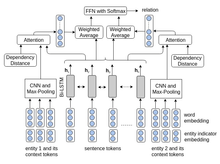
Figure 1: Architecture of our attention model with $m=1$. We have not shown the CNN-based global feature extraction here. FFN=feed-forward network.

3.2 Attention Modeling

Figure 1 shows the architecture of our attention model. We use a linear form of attention to find the semantically meaningful words in a sentence with respect to the entities which provide the pieces of evidence for the relation between them. Our attention mechanism uses the entities as attention queries and their vector representation is very important for our model. Named entities mostly consist of multiple tokens and many of them may not be present in the training data or their frequency may be low. The nearby words of an entity can give significant information about the entity. Thus we use the tokens of an entity and its nearby tokens to obtain its vector representation. We use the convolution operation with max-pooling in the context of an entity to get its vector representation.

$$c_{i}=\mathbf{f}^{T}(\mathbf{x}_{i}\|\mathbf{x}_{i+1}\|....\|\mathbf{x}_{i+k-1})$$

$$c_{max}=\mathrm{max}(c_{b},c_{b+1},....,c_{e})$$

$$\mathbf{v}_{e}=[c_{max}^{1},c_{max}^{2},....,c_{max}^{f_{e}}]$$

$\mathbf{f}$ is a convolutional filter vector of size $k(d_{w}+d_{z})$ where $k$ is the filter width and $\mathbf{x}$ is the concatenated vector of word embedding vector ($\mathbf{w}$) and entity token indicator embedding vector ($\mathbf{z}$). $b$ and $e$ are the start and end index of the sequence of words comprising an entity and its neighboring context in the sentence, where $1\leq b\leq e\leq n$. The index $i$ moves from $b$ to $e$ and produces a set of scalar values $\{c_{b},c_{b+1},.....,c_{e}\}$. The max-pooling operation chooses the maximum $c_{max}$ from these values as a feature. With $f_{e}$ number of filters, we get the entity vector $\mathbf{v}_{e}\in\mathbb{R}^{f_{e}}$. We do this for both entities and get $\mathbf{v}_{e}^{1}\in\mathbb{R}^{f_{e}}$ and $\mathbf{v}_{e}^{2}\in\mathbb{R}^{f_{e}}$ as their vector representation. We adopt a simple linear function as follows to measure the semantic similarity of words with the given entities:

$$\mathrm{f_{score}^{1}}(\mathbf{h}_{i},\mathbf{v}_{e}^{1})=\mathbf{h}_{i}^{T}\mathbf{W}_{a}^{1}\mathbf{v}_{e}^{1}$$

$$\mathrm{f_{score}^{2}}(\mathbf{h}_{i},\mathbf{v}_{e}^{2})=\mathbf{h}_{i}^{T}\mathbf{W}_{a}^{2}\mathbf{v}_{e}^{2}$$

$\mathbf{h}_{i}$ is the Bi-LSTM hidden representation of the $i$th word. $\mathbf{W}_{a}^{1},\mathbf{W}_{a}^{2}\in\mathbb{R}^{2(d_{w}+d_{z})\times f_{e}}$ are trainable weight matrices. $\mathrm{f_{score}^{1}}(\mathbf{h}_{i},\mathbf{v}_{e}^{1})$ and $\mathrm{f_{score}^{2}}(\mathbf{h}_{i},\mathbf{v}_{e}^{2})$ represent the semantic similarity score of the $i$th word and the two given entities.

Not all words in a sentence are equally important in finding the relation between the two entities. The words which are closer to the entities are generally more important. To address this issue, we propose to incorporate the syntactic structure of a sentence in our attention mechanism. The syntactic structure is obtained from the dependency parse tree of the sentence. Words which are closer to the entities in the dependency parse tree are more relevant to finding the relation. In our model, we define the dependency distance to every word from the head token (last token) of an entity as the number of edges along the dependency path (See Figure 2 for an example). We use a distance window size $ws$ and words whose dependency distance is within this window receive attention and the other words are ignored. The details of our attention mechanism follow.

$$d_{i}^{1}=\begin{cases}\frac{1}{2^{l_{i}^{1}-1}}\mathrm{exp(f_{score}^{1}}(\mathbf{h}_{i},\mathbf{v}_{e}^{1}))&\text{if }l_{i}^{1}\in[1,ws]\\ \frac{1}{2^{ws}}\mathrm{exp(f_{score}^{1}}(\mathbf{h}_{i},\mathbf{v}_{e}^{1}))&\text{otherwise}\end{cases}$$

$$d_{i}^{2}=\begin{cases}\frac{1}{2^{l_{i}^{2}-1}}\mathrm{exp(f_{score}^{2}}(\mathbf{h}_{i},\mathbf{v}_{e}^{2}))&\text{if }l_{i}^{2}\in[1,ws]\\ \frac{1}{2^{ws}}\mathrm{exp(f_{score}^{2}}(\mathbf{h}_{i},\mathbf{v}_{e}^{2}))&\text{otherwise}\end{cases}$$

$$p_{i}^{1}=\frac{d_{i}^{1}}{\sum_{j}{d_{j}^{1}}},\quad\quad\quad\quad p_{i}^{2}=\frac{d_{i}^{2}}{\sum_{j}{d_{j}^{2}}}$$

$d_{i}^{1}$ and $d_{i}^{2}$ are un-normalized attention scores and $p_{i}^{1}$ and $p_{i}^{2}$ are the normalized attention scores for the $i$th word with respect to entity 1 and entity 2 respectively. $l_{i}^{1}$ and $l_{i}^{2}$ are the dependency distances of the $i$th word from the two entities. We mask those words whose average dependency distance from the two entities is larger than $ws$. We use the semantic meaning of the words and their dependency distance from the two entities together in our attention mechanism. The attention feature vectors $\mathbf{v}_{a}^{1}$ and $\mathbf{v}_{a}^{1}$ with respect to the two entities are determined as follows:

$$\mathbf{v}_{a}^{1}=\sum_{i=1}^{n}p_{i}^{1}\mathbf{h}_{i},\quad\quad\mathbf{v}_{a}^{2}=\sum_{i=1}^{n}p_{i}^{2}\mathbf{h}_{i}$$

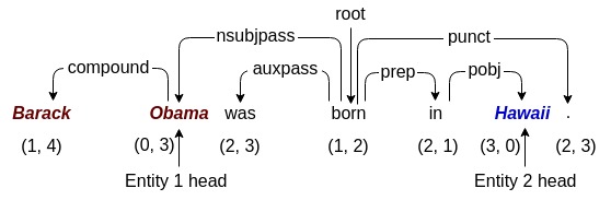
Figure 2: An example dependency tree. The two numbers indicate the distance of the word from the head token of the two entities respectively along the dependency tree path.

3.3 Multi-Factor Attention

Two entities in a sentence, when located far from each other, can be linked via more than one co-reference chain or more than one important word. Due to the normalization of the attention scores as described above, single attention cannot capture all relevant information needed to find the relation between two entities. Thus we use a multi-factor attention mechanism, where the number of factors is a hyper-parameter, to gather all relevant information for identifying the relation. We replace the attention matrix $\mathbf{W}_{a}$ with an attention tensor $\mathbf{W}_{a}^{1:m}\in\mathbb{R}^{m\times 2(d_{w}+d_{z})\times 2f_{e}}$ where $m$ is the factor count. This gives us $m$ attention vectors with respect to each entity. We concatenate all the feature vectors obtained using these attention vectors to get the multi-attentive feature vector $\mathbf{v}_{ma}\in\mathbb{R}^{4m(d_{w}+d_{z})}$.

3.4 Relation Extraction

We concatenate $\mathbf{v}_{g}$, $\mathbf{v}_{ma}$, $\mathbf{v}_{e}^{1}$, and $\mathbf{v}_{e}^{2}$, and this concatenated feature vector is given to a feed-forward layer with softmax activation to predict the normalized probabilities for the relation labels.

$$\mathbf{r}=\mathrm{softmax}(\mathbf{W}_{r}(\mathbf{v}_{g}~{}||~{}\mathbf{v}_{ma}~{}||~{}\mathbf{v}_{e}^{1}~{}||~{}\mathbf{v}_{e}^{2})+\mathbf{b}_{r})$$

$\mathbf{W}_{r}\in\mathbb{R}^{(f_{g}+2f_{e}+4m(d_{w}+d_{z}))\times(|R|+1)}$ is the weight matrix, $\mathbf{b}_{r}\in\mathbb{R}^{|R|+1}$ is the bias vector of the feed-forward layer for relation extraction, and $\mathbf{r}$ is the vector of normalized probabilities of relation labels.

3.5 Loss Function

We calculate the loss over each mini-batch of size $B$. We use the following negative log-likelihood as our objective function for relation extraction:

$$\begin{split}\mathcal{L}=-\frac{1}{B}\sum_{i=1}^{B}\mathrm{log}(p(r_{i}|s_{i},e_{i}^{1},e_{i}^{2},\theta))\end{split}$$

where $p(r_{i}|s_{i},e_{i}^{1},e_{i}^{2},\theta)$ is the conditional probability of the true relation $r_{i}$ when the sentence $s_{i}$, two entities $e_{i}^{1}$ and $e_{i}^{2}$, and the model parameters $\theta$ are given.

4 Experiments

4.1 Datasets

We use the New York Times (NYT) corpus Riedel et al. (2010) in our experiments. There are two versions of this corpus: (1) The original NYT corpus created by Riedel et al. (2010) which has $52$ valid relations and a None relation. We name this dataset NYT10. The training dataset has $455,412$ instances and $330,776$ of the instances belong to the None relation and the remaining $124,636$ instances have valid relations. The test dataset has $172,415$ instances and $165,974$ of the instances belong to the None relation and the remaining $6,441$ instances have valid relations. Both the training and test datasets have been created by aligning Freebase Bollacker et al. (2008) tuples to New York Times articles. (2) Another version created by Hoffmann et al. (2011) which has $24$ valid relations and a None relation. We name this dataset NYT11. The corresponding statistics for NYT11 are given in Table 1. The training dataset is created by aligning Freebase tuples to NYT articles, but the test dataset is manually annotated.

		NYT10	NYT11
	# relations	53	25
Train	# instances	455,412	335,843
	# valid relation tuples	124,636	100,671
	# None relation tuples	330,776	235,172
	avg. sentence length	41.1	37.2
	avg. distance between entity pairs	12.8	12.2
Test	# instances	172,415	1,450
	# valid relation tuples	6,441	520
	# None relation tuples	165,974	930
	avg. sentence length	41.7	39.7
	avg. distance between entity pairs	13.1	11.0

Table 1: Statistics of the NYT10 and NYT11 dataset.

4.2 Evaluation Metrics

We use precision, recall, and F1 scores to evaluate the performance of models on relation extraction after removing the None labels. We use a confidence threshold to decide if the relation of a test instance belongs to the set of relations $R$ or None. If the network predicts None for a test instance, then it is considered as None only. But if the network predicts a relation from the set $R$ and the corresponding softmax score is below the confidence threshold, then the final class is changed to None. This confidence threshold is the one that achieves the highest F1 score on the validation dataset. We also include the precision-recall curves for all the models.

4.3 Parameter Settings

We run word2vec Mikolov et al. (2013) on the NYT corpus to obtain the initial word embeddings with dimension $d_{w}=50$ and update the embeddings during training. We set the dimension of entity token indicator embedding vector $d_{z}=10$ and positional embedding vector $d_{u}=5$. The hidden layer dimension of the forward and backward LSTM is $60$, which is the same as the dimension of input word representation vector $\mathbf{x}$. The dimension of Bi-LSTM output is $120$. We use $f_{g}=f_{e}=230$ filters of width $k=3$ for feature extraction whenever we apply the convolution operation. We use dropout in our network with a dropout rate of $0.5$, and in convolutional layers, we use the tanh activation function. We use the sequence of tokens starting from $5$ words before the entity to $5$ words after the entity as its context. We train our models with mini-batch size of $50$ and optimize the network parameters using the Adagrad optimizer Duchi et al. (2011). We use the dependency parser from spaCy to obtain the dependency distance of the words from the entities and use $ws=5$ as the window size for dependency distance-based attention.

	NYT10			NYT11
Model	Prec.	Rec.	F1	Prec.	Rec.	F1
CNN Zeng et al. (2014)	0.413	0.591	0.486	0.444	0.625	0.519
PCNN Zeng et al. (2015)	0.380	0.642	0.477	0.446	0.679	0.538†
EA Shen and Huang (2016)	0.443	0.638	0.523†	0.419	0.677	0.517
BGWA Jat et al. (2017)	0.364	0.632	0.462	0.417	0.692	0.521
BiLSTM-CNN	0.490	0.507	0.498	0.473	0.606	0.531
Our model	0.541	0.595	0.566*	0.507	0.652	0.571*

Table 2: Performance comparison of different models on the two datasets. * denotes a statistically significant improvement over the previous best state-of-the-art model with $p<0.01$ under the bootstrap paired t-test. ^† denotes the previous best state-of-the-art model.

4.4 Comparison to Prior Work

We compare our proposed model with the following state-of-the-art models.

(1) CNN Zeng et al. (2014): Words are represented using word embeddings and two positional embeddings. A convolutional neural network (CNN) with max-pooling is applied to extract the sentence-level feature vector. This feature vector is passed to a feed-forward layer with softmax to classify the relation.

(2) PCNN Zeng et al. (2015): Words are represented using word embeddings and two positional embeddings. A convolutional neural network (CNN) is applied to the word representations. Rather than applying a global max-pooling operation on the entire sentence, three max-pooling operations are applied on three segments of the sentence based on the location of the two entities (hence the name Piecewise Convolutional Neural Network (PCNN)). The first max-pooling operation is applied from the beginning of the sentence to the end of the entity appearing first in the sentence. The second max-pooling operation is applied from the beginning of the entity appearing first in the sentence to the end of the entity appearing second in the sentence. The third max-pooling operation is applied from the beginning of the entity appearing second in the sentence to the end of the sentence. Max-pooled features are concatenated and passed to a feed-forward layer with softmax to determine the relation.

(3) Entity Attention (EA) Shen and Huang (2016): This is the combination of a CNN model and an attention model. Words are represented using word embeddings and two positional embeddings. A CNN with max-pooling is used to extract global features. Attention is applied with respect to the two entities separately. The vector representation of every word is concatenated with the word embedding of the last token of the entity. This concatenated representation is passed to a feed-forward layer with tanh activation and then another feed-forward layer to get a scalar attention score for every word. The original word representations are averaged based on the attention scores to get the attentive feature vectors. A CNN-extracted feature vector and two attentive feature vectors with respect to the two entities are concatenated and passed to a feed-forward layer with softmax to determine the relation.

(4) BiGRU Word Attention (BGWA) Jat et al. (2017): Words are represented using word embeddings and two positional embeddings. They are passed to a bidirectional gated recurrent unit (BiGRU) Cho et al. (2014) layer. Hidden vectors of the BiGRU layer are passed to a bilinear operator (a combination of two feed-forward layers) to compute a scalar attention score for each word. Hidden vectors of the BiGRU layer are multiplied by their corresponding attention scores. A piece-wise CNN is applied on the weighted hidden vectors to obtain the feature vector. This feature vector is passed to a feed-forward layer with softmax to determine the relation.

(5) BiLSTM-CNN: This is our own baseline. Words are represented using word embeddings and entity indicator embeddings. They are passed to a bidirectional LSTM. Hidden representations of the LSTMs are concatenated with two positional embeddings. We use CNN and max-pooling on the concatenated representations to extract the feature vector. Also, we use CNN and max-pooling on the word embeddings and entity indicator embeddings of the context words of entities to obtain entity-specific features. These features are concatenated and passed to a feed-forward layer to determine the relation.

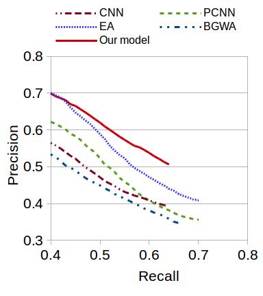
Figure 3: Precision-Recall curve for the NYT10 dataset.

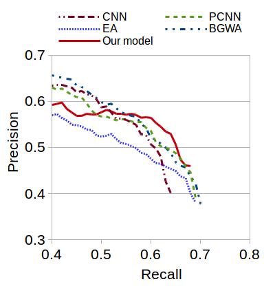
Figure 4: Precision-Recall curve for the NYT11 dataset.

4.5 Experimental Results

We present the results of our final model on the relation extraction task on the two datasets in Table 2. Our model outperforms the previous state-of-the-art models on both datasets in terms of F1 score. On the NYT10 dataset, it achieves $4.3\%$ higher F1 score compared to the previous best state-of-the-art model EA. Similarly, it achieves $3.3\%$ higher F1 score compared to the previous best state-of-the-model PCNN on the NYT11 dataset. Our model improves the precision scores on both datasets with good recall scores. This will help to build a cleaner knowledge base with fewer false positives. We also show the precision-recall curves for the NYT10 and NYT11 datasets in Figures 3 and 4 respectively. The goal of any relation extraction system is to extract as many relations as possible with minimal false positives. If the recall score becomes very low, the coverage of the KB will be poor. From Figure 3, we observe that when the recall score is above $0.4$, our model achieves higher precision than all the competing models on the NYT10 dataset. On the NYT11 dataset (Figure 4), when recall score is above $0.6$, our model achieves higher precision than the competing models. Achieving higher precision with high recall score helps to build a cleaner KB with good coverage.

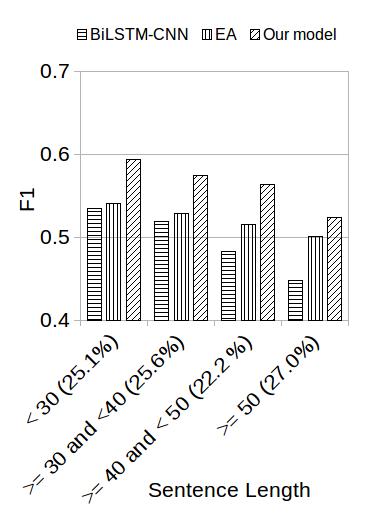
Figure 5: Performance comparison across different sentence lengths on the NYT10 dataset.

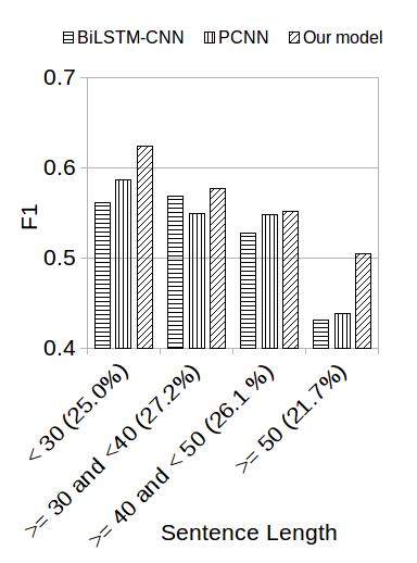
Figure 6: Performance comparison across different sentence lengths on the NYT11 dataset.

5 Analysis and Discussion

5.1 Varying the number of factors ($m$)

We investigate the effects of the multi-factor count $(m)$ in our final model on the test datasets in Table 3. We observe that for the NYT10 dataset, $m=\{1,2,3\}$ gives good performance with $m=1$ achieving the highest F1 score. On the NYT11 dataset, $m=4$ gives the best performance. These experiments show that the number of factors giving the best performance may vary depending on the underlying data distribution.

	NYT10			NYT11
$m$	Prec.	Rec.	F1	Prec.	Rec.	F1
${1}$	0.541	0.595	0.566	0.495	0.621	0.551
${2}$	0.521	0.597	0.556	0.482	0.656	0.555
${3}$	0.490	0.617	0.547	0.509	0.633	0.564
${4}$	0.449	0.623	0.522	0.507	0.652	0.571
${5}$	0.467	0.609	0.529	0.488	0.677	0.567

Table 3: Performance comparison of our model with different values of $m$ on the two datasets.

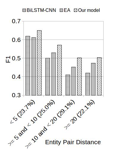
Figure 7: Performance comparison across different distances between entities on the NYT10 dataset.

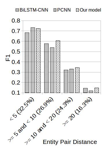
Figure 8: Performance comparison across different distances between entities on the NYT11 dataset.

5.2 Effectiveness of Model Components

We include the ablation results on the NYT11 dataset in Table 4. When we add multi-factor attention to the baseline BiLSTM-CNN model without the dependency distance-based weight factor in the attention mechanism, we get $0.8\%$ F1 score improvement (A2$-$A1). Adding the dependency weight factor with a window size of $5$ improves the F1 score by $3.2\%$ (A3$-$A2). Increasing the window size to $10$ reduces the F1 score marginally (A3$-$A4). Replacing the attention normalizing function with softmax operation also reduces the F1 score marginally (A3$-$A5). In our model, we concatenate the features extracted by each attention layer. Rather than concatenating them, we can apply max-pooling operation across the multiple attention scores to compute the final attention scores. These max-pooled attention scores are used to obtain the weighted average vector of Bi-LSTM hidden vectors. This affects the model performance negatively and F1 score of the model decreases by $3.0\%$ (A3$-$A6).

	Prec.	Rec.	F1
(A1) BiLSTM-CNN	0.473	0.606	0.531
(A2) Standard attention	0.466	0.638	0.539
(A3) Window size $(ws)=5$	0.507	0.652	0.571
(A4) Window size $(ws)=10$	0.510	0.640	0.568
(A5) Softmax	0.490	0.658	0.562
(A6) Max-pool	0.492	0.600	0.541

Table 4: Effectiveness of model components ($m=4$) on the NYT11 dataset.

5.3 Performance with Varying Sentence Length and Varying Entity Pair Distance

We analyze the effects of our attention model with different sentence lengths in the two datasets in Figures 5 and 6. We also analyze the effects of our attention model with different distances between the two entities in the two datasets in Figures 7 and 8. We observe that with increasing sentence length and increasing distance between the two entities, the performance of all models drops. This shows that finding the relation between entities located far from each other is a more difficult task. Our multi-factor attention model with dependency-distance weight factor increases the F1 score in all configurations when compared to previous state-of-the-art models on both datasets.

6 Related Work

Relation extraction from a distantly supervised dataset is an important task and many researchers Mintz et al. (2009); Riedel et al. (2010); Hoffmann et al. (2011) tried to solve this task using feature-based classification models. Recently, Zeng et al. (2014, 2015) used CNN models for this task which can extract features automatically. Shen and Huang (2016) and Jat et al. (2017) used attention mechanism in their model to improve performance. Surdeanu et al. (2012), Lin et al. (2016), Vashishth et al. (2018), Wu et al. (2019), and Ye and Ling (2019) used multiple sentences in a multi-instance relation extraction setting to capture the features located in multiple sentences for a pair of entities. In their evaluation setting, they evaluated model performance by considering multiple sentences having the same pair of entities as a single test instance. On the other hand, our model and the previous models that we compare to in this paper Zeng et al. (2014, 2015); Shen and Huang (2016); Jat et al. (2017) work on each sentence independently and are evaluated at the sentence level. Since there may not be multiple sentences that contain a pair of entities, it is important to improve the task performance at the sentence level. Future work can explore the integration of our sentence-level attention model in a multi-instance relation extraction framework.

Not much previous research has exploited the dependency structure of a sentence in different ways for relation extraction. Xu et al. (2015) and Miwa and Bansal (2016) used an LSTM network and the shortest dependency path between two entities to find the relation between them. Huang et al. (2017) used the dependency structure of a sentence for the slot-filling task which is close to the relation extraction task. Liu et al. (2015) exploited the shortest dependency path between two entities and the sub-trees attached to that path (augmented dependency path) for relation extraction. Zhang et al. (2018) and Guo et al. (2019) used graph convolution networks with pruned dependency tree structures for this task. In this work, we have incorporated the dependency distance of the words in a sentence from the two entities in a multi-factor attention mechanism to improve sentence-level relation extraction.

Attention-based neural networks are quite successful for many other NLP tasks. Bahdanau et al. (2015) and Luong et al. (2015) used attention models for neural machine translation, Seo et al. (2017) used attention mechanism for answer span extraction. Vaswani et al. (2017) and Kundu and Ng (2018) used multi-head or multi-factor attention models for machine translation and answer span extraction respectively. He et al. (2018) used dependency distance-focused word attention model for aspect-based sentiment analysis.

7 Conclusion

In this paper, we have proposed a multi-factor attention model utilizing syntactic structure for relation extraction. The syntactic structure component of our model helps to identify important words in a sentence and the multi-factor component helps to gather different pieces of evidence present in a sentence. Together, these two components improve the performance of our model on this task, and our model outperforms previous state-of-the-art models when evaluated on the New York Times (NYT) corpus, achieving significantly higher F1 scores.

References

- Bahdanau et al. (2015) Dzmitry Bahdanau, Kyunghyun Cho, and Yoshua Bengio. 2015. Neural machine translation by jointly learning to align and translate. In Proceedings of the International Conference on Learning Representations.
- Banko et al. (2007) Michele Banko, Michael J Cafarella, Stephen Soderland, Matthew Broadhead, and Oren Etzioni. 2007. Open information extraction from the web. In Proceedings of the International Joint Conference on Artificial Intelligence.
- Bollacker et al. (2008) Kurt Bollacker, Colin Evans, Praveen Paritosh, Tim Sturge, and Jamie Taylor. 2008. Freebase: A collaboratively created graph database for structuring human knowledge. In Proceedings of the ACM SIGMOD International Conference on Management of Data.
- Cho et al. (2014) Kyunghyun Cho, Bart Van Merriënboer, Dzmitry Bahdanau, and Yoshua Bengio. 2014. On the properties of neural machine translation: Encoder-decoder approaches. In Proceedings of Eighth Workshop on Syntax, Semantics and Structure in Statistical Translation.
- Duchi et al. (2011) John Duchi, Elad Hazan, and Yoram Singer. 2011. Adaptive subgradient methods for online learning and stochastic optimization. Journal of Machine Learning Research.
- Guo et al. (2019) Zhijiang Guo, Yan Zhang, and Wei Lu. 2019. Attention guided graph convolutional networks for relation extraction. In Proceedings of the 57nd Annual Meeting of the Association for Computational Linguistics.
- He et al. (2018) Ruidan He, Wee Sun Lee, Hwee Tou Ng, and Daniel Dahlmeier. 2018. Effective attention modeling for aspect-level sentiment classification. In Proceedings of the 27th International Conference on Computational Linguistics.
- Hochreiter and Schmidhuber (1997) Sepp Hochreiter and Jürgen Schmidhuber. 1997. Long short-term memory. Neural Computation.
- Hoffmann et al. (2011) Raphael Hoffmann, Congle Zhang, Xiao Ling, Luke Zettlemoyer, and Daniel S Weld. 2011. Knowledge-based weak supervision for information extraction of overlapping relations. In Proceedings of the 49th Annual Meeting of the Association for Computational Linguistics.
- Huang et al. (2017) Lifu Huang, Avirup Sil, Heng Ji, and Radu Florian. 2017. Improving slot filling performance with attentive neural networks on dependency structures. In Proceedings of the 2017 Conference on Empirical Methods in Natural Language Processing.
- Jat et al. (2017) Sharmistha Jat, Siddhesh Khandelwal, and Partha Talukdar. 2017. Improving distantly supervised relation extraction using word and entity based attention. In Proceedings of the 6th Workshop on Automated Knowledge Base Construction.
- Kundu and Ng (2018) Souvik Kundu and Hwee Tou Ng. 2018. A question-focused multi-factor attention network for question answering. In Proceedings of the Association for the Advancement of Artificial Intelligence.
- Lin et al. (2016) Yankai Lin, Shiqi Shen, Zhiyuan Liu, Huanbo Luan, and Maosong Sun. 2016. Neural relation extraction with selective attention over instances. In Proceedings of the 54th Annual Meeting of the Association for Computational Linguistics.
- Liu et al. (2015) Yang Liu, Furu Wei, Sujian Li, Heng Ji, Ming Zhou, and Houfeng Wang. 2015. A dependency-based neural network for relation classification. In Proceedings of the 53rd Annual Meeting of the Association for Computational Linguistics and the 7th International Joint Conference on Natural Language Processing.
- Luong et al. (2015) Minh-Thang Luong, Hieu Pham, and Christopher D Manning. 2015. Effective approaches to attention-based neural machine translation. In Proceedings of the 2015 Conference on Empirical Methods in Natural Language Processing.
- Mikolov et al. (2013) Tomas Mikolov, Kai Chen, Greg Corrado, and Jeffrey Dean. 2013. Efficient estimation of word representations in vector space. In Proceedings of the International Conference on Learning Representations.
- Mintz et al. (2009) Mike Mintz, Steven Bills, Rion Snow, and Dan Jurafsky. 2009. Distant supervision for relation extraction without labeled data. In Proceedings of the 47th Annual Meeting of the Association for Computational Linguistics and the 4th International Joint Conference on Natural Language Processing.
- Miwa and Bansal (2016) Makoto Miwa and Mohit Bansal. 2016. End-to-end relation extraction using LSTMs on sequences and tree structures. In Proceedings of the 54th Annual Meeting of the Association for Computational Linguistics.
- Riedel et al. (2010) Sebastian Riedel, Limin Yao, and Andrew McCallum. 2010. Modeling relations and their mentions without labeled text. In Proceedings of the European Conference on Machine Learning and Knowledge Discovery in Databases.
- Seo et al. (2017) Minjoon Seo, Aniruddha Kembhavi, Ali Farhadi, and Hannaneh Hajishirzi. 2017. Bidirectional attention flow for machine comprehension. In Proceedings of the International Conference on Learning Representations.
- Shen and Huang (2016) Yatian Shen and Xuanjing Huang. 2016. Attention-based convolutional neural network for semantic relation extraction. In Proceedings of the 26th International Conference on Computational Linguistics.
- Surdeanu et al. (2012) Mihai Surdeanu, Julie Tibshirani, Ramesh Nallapati, and Christopher D. Manning. 2012. Multi-instance multi-label learning for relation extraction. In Proceedings of the 2012 Joint Conference on Empirical Methods in Natural Language Processing and Computational Natural Language Learning.
- Vashishth et al. (2018) Shikhar Vashishth, Rishabh Joshi, Sai Suman Prayaga, Chiranjib Bhattacharyya, and Partha Talukdar. 2018. Reside: Improving distantly-supervised neural relation extraction using side information. In Proceedings of the 2018 Conference on Empirical Methods in Natural Language Processing.
- Vaswani et al. (2017) Ashish Vaswani, Noam Shazeer, Niki Parmar, Jakob Uszkoreit, Llion Jones, Aidan N Gomez, Łukasz Kaiser, and Illia Polosukhin. 2017. Attention is all you need. In Proceedings of Advances in Neural Information Processing Systems.
- Wu et al. (2019) Shanchan Wu, Kai Fan, and Qiong Zhang. 2019. Improving distantly supervised relation extraction with neural noise converter and conditional optimal selector. In Proceedings of the Association for the Advancement of Artificial Intelligence.
- Xu et al. (2015) Yuning Xu, Lili Mou, Ge Li, Yunchuan Chen, Hao Peng, and Zhi Jin. 2015. Classifying relations via long short term memory networks along shortest dependency paths. In Proceedings of the 2015 Conference on Empirical Methods in Natural Language Processing.
- Ye and Ling (2019) Zhi-Xiu Ye and Zhen-Hua Ling. 2019. Distant supervision relation extraction with intra-bag and inter-bag attentions. In Proceedings of the 2019 Conference of the North American Chapter of the Association for Computational Linguistics.
- Zeng et al. (2015) Daojian Zeng, Kang Liu, Yubo Chen, and Jun Zhao. 2015. Distant supervision for relation extraction via piecewise convolutional neural networks. In Proceedings of the 2015 Conference on Empirical Methods in Natural Language Processing.
- Zeng et al. (2014) Daojian Zeng, Kang Liu, Siwei Lai, Guangyou Zhou, and Jun Zhao. 2014. Relation classification via convolutional deep neural network. In Proceedings of the 25th International Conference on Computational Linguistics.
- Zhang et al. (2018) Yuhao Zhang, Peng Qi, and Christopher D. Manning. 2018. Graph convolution over pruned dependency trees improves relation extraction. In Proceedings of the 2018 Conference on Empirical Methods in Natural Language Processing.