DG Approach to Large Bending Plate Deformations with Isometry Constraint
Abstract.
We propose a new discontinuous Galerkin (dG) method for a geometrically nonlinear Kirchhoff plate model for large isometric bending deformations. The minimization problem is nonconvex due to the isometry constraint. We present a practical discrete gradient flow that decreases the energy and computes discrete minimizers that satisfy a prescribed discrete isometry defect. We prove -convergence of the discrete energies and discrete global minimizers. We document the flexibility and accuracy of the dG method with several numerical experiments.
Key words and phrases:
Nonlinear elasticity; plate bending; isometry constraint; discontinuous Galerkin; iterative solution; -convergence.1. Introduction
Large bending deformations of thin plates is a critical feature for many modern engineering applications due to the extensive use of plate actuators in a variety of systems like thermostats, nano-tubes, micro-robots and micro-capsules [9, 24, 27, 33, 34]. From the mathematical viewpoint, there is an increasing interest in the modeling and the numerical treatment of such plates. A rigorous analysis of large bending deformations of plates was conducted by Friesecke, James and Müller [23], who derived the geometrically non-linear Kirchhoff model from three dimensional hyperelasticity via -convergence. Since then, there have been various other interesting models, such as the models of prestrained plates derived in [10, 28]. Previous work on the numerical treatment of large bending deformations includes the single layer problem by Bartels [5], the bilayer problem by Bartels, Bonito and Nochetto [8] and the modeling and simulation of thermally actuated bilayer plates by Bartels, Bonito, Muliana and Nochetto [7]. In all three approaches [5, 7, 8] the model involves minimizing an energy functional that is dominated by the Hessian of the deformation of the mid-plane of the undeformed plate. Given functions , the minimization takes place under Dirichlet boundary conditions for and on part of the boundary of and the isometry constraint
| (1.1) |
where stands for the identity matrix in . The authors of [5, 7, 8] employ Kirchhoff elements in order to impose the isometry constraint at the nodes of the triangulation and rely on an - gradient flow that allows them to construct solutions of decreasing discrete energy. In [5, 8] it is also proved that the discrete energy -converges to the continuous one. Since for fourth order problems a conforming approach would be very costly, the Kirchhoff elements offer a natural non-conforming space for the model that allows the imposition of (1.1) nodewise.
1.1. Our contribution
In this paper we focus on the single layer problem, as in [5], in order to investigate the applicability of a more flexible approach that hinges on a non-conforming space of discontinuous functions. We use interior penalty terms for the discrete energy along with a Nitsche’s approach to enforce the boundary conditions in the limit. We start with the Dirichlet and forcing data
| (1.2) |
and the affine manifold of
| (1.3) |
where is an open non-empty subset of the boundary . We wish to approximate a minimizer of the continuous energy
| (1.4) |
in the nonconvex set of admissible functions
| (1.5) |
where denotes the Frobenius norm. To avoid the costly use of a conforming finite element subspace of , we resort to a space of discontinuous piecewise polynomials of degree over a shape-regular but possibly graded mesh (constructed either using the reference unit triangle or unit square). Since our estimates below are all local, hereafter stands for a mesh density function locally equivalent to the element size. However, to de-emphasize this aspect of our approach in favor of others (non-convexity, Hessian reconstruction, -convergence) and to simplify notation, written as a parameter signifies the meshsize of (i.e. the largest element size). We denote by the discrete energy that approximates and accounts for the discontinuities of the functions and of their broken (i.e. piecewise) gradients ; see (2.16).
It is important to notice that the energy in (1.4) is convex but the isometry constraint (1.1) is not. Therefore, we must approximate (1.1), and thus the admissible set in a way amenable to computation, as well as construct an algorithm able to find critical points. We define the discrete admissible set to be the set of functions whose boundary jumps include and (see (2.9) and (2.10) below) and whose discrete isometry defect satisfies
| (1.6) |
where as . We then search for that minimizes the discrete energy . To this end, we propose a discrete -gradient flow with fictitious time step that can be made arbitrarily small. We show that it gives rise to iterates with decreasing discrete energy , whenever , and guarantees the discrete isometry defect (1.6) for all provided the initial guess is an approximate isometry such that . This is achieved by selecting proportional to , depending on .
We also prove -convergence of the discrete energy to the continuous energy and that global minimizers of converge in to global minimizers of as . A key ingredient for -convergence is reconstruction of a suitable discrete Hessian of , which uses the broken Hessian and the jumps and of and across interelement boundaries. Such is an -function in that converges weakly to under suitable mesh conditions. A similar approach is employed in [20] for second order problems and later in [31] for the biharmonic equation, where . We refer to Section 4 for a discussion of properties of and critical differences with [20, 31].
Our approach is motivated by the flexibility of dG compared to Kirchhoff elements [5, 6]. First of all, Kirchhoff elements require polynomial degree and suffer from a complicated implementation that involves a discrete gradient that maps the gradient of the discrete deformation to another space. Since this is not implemented in standard finite element libraries, the above difficulty hinders the impact of the method in the engineering community. In contrast, the proposed dG approach works for , does not require such map (or more precisely, the map is the trivial elementwise differentiation) and its implementation is standard. Moreover, quadrilateral Kirchhoff elements are not amenable to adaptively refined partitions, at least in theory; the current dG theory, instead, allows for graded meshes . It is worth mentioning as well that imposing Dirichlet boundary conditions weakly, instead of directly in the admissible set as in [5, 6, 8, 7], allows for more flexibility. In particular, this alleviates the constraints on the construction of the recovery sequence necessary for the -convergence of towards ; see Section 5.3. Upon dropping the penalty term of jumps of across a prescribed curve, dG naturally accommodates configurations with kinks, as is the case of origami. Lastly, imposing the isometry constraint numerically with Kirchhoff elements at each vertex seems to be very rigid at the expense of approximation accuracy. In contrast, our experiments with dG indicate that this approach is more accurate and adjusts better to the geometry of the problem; see Section 6.1.
1.2. Outline
We first construct our discrete energy functional in Section 2, and prove key properties for functions , including the coercivity of with respect to an appropriate mesh-dependent energy norm. We introduce in Section 3 the discrete -gradient flow and show it is able to find discrete minimizers of that satisfy the desired discrete isometry defect (1.6); this sets the stage for relations between and in (1.6). In Section 4 we define the discrete Hessian and derive a bound in and its weak convergence in . This leads to the proof of -convergence of the discrete energy to the exact energy , in Section 5, as well as the convergence of global minimizers of to global minimizers of . In Section 6 we present experiments that corroborate numerically the excellent properties of our method and compare it with the Kirchhoff element approach. In Section 7 we provide some details for our implementation and justify the choice of a discontinuous versus a continuous space of functions . We draw conclusions in Section 8 and present some technical estimates for isoparametric maps in the appendix of Section 9.
2. Discrete Energy and Properties of dG
We start this section by providing intuition on the derivation of the discrete energy , but without presenting all the details. We then introduce the discrete dG space for scalar functions along with an interpolation operator , and discuss its properties. We finally prove coercivity of .
2.1. Continuous energy
Starting from a three-dimensional hyperelasticity model, dimension reduction as the thickness of the plate decreases to zero leads to the two-dimensional energy functional [5, 6, 23]
| (2.1) |
up to a multiplicative constant for the first term. Hereafter, is an isometric deformation from into , is the unit normal and is the second fundamental form of the deformed plate . The connection between (2.1) and (1.4) follows from (1.1), namely
where is the Kronecker delta. Differentiating with respect to the cartesian coordinates and and using simple algebraic manipulations, these relations imply
This, combined with the definition , leads in turn to
Similarly, using that
we obtain
Therefore, the isometry property (1.1) yields the pointwise relations
| (2.2) |
so that the nonlinear expression (2.1) of coincides with (1.4), namely
| (2.3) |
The Euler-Lagrange equation for a minimizer of (2.3) reads
| (2.4) |
where is defined in (1.3). If , then the strong form of (2.4) is
| (2.5) |
whereas the natural boundary conditions imposed on are
| (2.6) |
Hereafter, denotes the outward unit normal to .
2.2. Discrete energy
We denote by (resp. ) the space of polynomial functions of degree at most (resp. at most on each variable). Moreover, stands for the reference element, which is either the unit triangle for or the unit square for . A generic element is given by a map (resp. ) provided is the unit triangle (resp. square). Notice that when , is affine for triangles and bi-linear for quadrilaterals .
We consider a sequence of meshes of made of closed shape regular but possibly graded elements [19]. We assume that can be exactly represented by such subdivisions, i.e. we do not account in the analysis below for variational crimes induced by the approximation of the boundary . Hereafter, we denote by a mesh density function which is equivalent locally to the size of and of an edge ; written as a parameter also signifies the largest value of . In order to handle hanging nodes (necessary for graded meshes based on quadrilaterals), we assume that all the elements within each domain of influence have comparable diameters (independently of ). We refer to Sections 2.2.4 and 6 of Bonito-Nochetto [11] for precise definitions and properties. At this point, we only point out that sequences of meshes made of quadrilaterals with at most one hanging node per side satisfy this assumption. We append a sub-index to differential operators to indicate that they are applied element-wise. For instance, is defined by , .
From now on and are generic constants independent of but perhaps depending on the shape-regularity constant of the mesh sequence . Also, we use the notation to indicate , where is a constant independent of , and .
Let be the space of discontinuous functions over the mesh
| (2.7) |
of degree . We point out that the discrete functions are not polynomials on the physical elements unless . This is consistent with the implementation in the deal.ii library[1] used to obtain the numerical illustrations of Section 6. Similarly, the Hessians of and are not proportional because , except when . We account for this delicate issue in Section 9.
We denote by the collection of edges of contained in and by those contained in ; hence is the set of active interelement boundaries. We further denote the interior skeleton and the boundary counterpart by
| (2.8) |
and by the full skeleton.
As is customary for dG methods, we need to introduce jumps and averages on edges. For we fix to be one of the two unit normals to in ; this choice is irrelevant for the discussion below. Given , we denote its broken gradient by and the jumps of and across interior edges by
| (2.9) |
where and . In order to deal with Dirichlet boundary data we resort to a Nitsche’s approach; hence we do not impose essential restrictions on the discrete space . However, to simplify the notation later it turns out to be convenient to introduce the discrete sets and which mimic the continuous counterparts and but coincide with . In fact, we say that belongs to provided the boundary jumps of are defined to be
| (2.10) |
We stress that and imply and in as ; hence the connection between and . Therefore, the sets and coincide but the latter is not a space because it carries the additional information of boundary jumps, namely
| (2.11) |
In the same vein, we will deal with discrete test functions for which boundary jumps are given by and for all , which is consistent with (2.10) for , . We observe again that the sets and are the same. We will not write the subscript whenever no confusion arises. On the other hand, the definiton of average of across an edge is independent of Dirichlet conditions and is thus given by
| (2.12) |
Definitions (2.9), (2.10) and (2.12) extend to the broken energy space
| (2.13) |
Before introducing the discrete energy , we derive the corresponding bilinear form in the usual manner. This is the first instance where the definitions of and become critical. We integrate by parts twice the strong equation (2.5) over elements against a test function . We assume to be smooth, whence the jumps and vanish on edges , to arrive at
We next use that and for all edges : for interior edges this is because is smooth, whereas for boundary edges it is a consequence of and on and definition (2.10). We can thus symmetrize the previous equality and add vanishing penalty terms
| (2.14) | ||||
with penalty parameters to be determined. Hereafter, we denote by the scalar product and vector versions of it. Since (2.14) reduces to (2.4) for , we resort to (2.14) to define the discrete equation for
| (2.15) |
We point out that the Dirichlet conditions in (1.3) are enforced in the Nitsche’s sense. Since is symmetric by construction, we define the discrete energy to be
| (2.16) |
The first variation of in the direction yields (2.15).
In order for (2.16) to be meaningful with respect to the original minimization problem in (1.4)-(1.5), we define the discrete admissible set , a discrete analogue of in (1.5) that involves the discrete isometry defect , to be
| (2.17) |
with parameter as . We will see in Section 3 that the discrete gradient flow used to construct discrete solutions yields , where depends on , being the initial iterate, and other geometric constants.
2.3. Interpolation onto Continuous Piecewise Polynomials
For several reasons we need to interpolate from the broken energy space defined in (2.13) onto the space of continuous functions which are polynomials of degree over the reference element . We refer to [3, 11, 13, 15, 17] for such interpolation estimates. We now construct a Clément type interpolation operator , thereby extending [3, 11] to , because of its simplicity and fitness with our application of it.
We construct in two steps. We first compute the local -projection , which for every and reduces to the equation
| (2.18) |
where (resp. ) stands for the restriction of functions in (resp. ) to . We next define the Clément interpolation operator of [3, 11] as follows. Given the canonical basis functions of with supports associated with nodes , we compute the -projection of on stars
| (2.19) |
and define and
| (2.20) |
If has hanging nodes, the stars are related to the notion of domain of influence; we refer to Section 6 of [11] for details. We make the same assumptions as [11] on , which in turn imply that all elements of within possess comparable size.
Lemma 2.1 (interpolation).
Proof.
The operator is invariant in because so are and . We next examine properties of , and separately. Recall that all are closed.
Step 1: Operator . Since is an elementwise -projection, we easily deduce
Given an interior edge , let be the two adjacent elements that satisfy and be the restrictions of to . If , a simple calculation now shows
Step 2: Operator . Let be the union of stars alluded to in (2.19) that intersect ; note that all elements within have comparable size [11]. Moreover, let and be the skeletons of and (interelement boundaries internal to these sets). We recall (see e.g. [11]) that to prove the estimate
for all , it suffices to derive the bounds
where is defined in (2.19). Since the dimension of the space is finite and depends only on shape regularity, all norms in are equivalent and independent of meshsize upon rescaling to unit size. We further observe that if the right hand side of the last inequality vanishes, then is constant in . The definition of thus gives and the left hand side vanishes, thereby showing that the desired estimate is valid in the rescaled . The powers of meshsize result from a standard scaling argument from unit size back to actual size.
Step 3: Operator . Combining the estimates for and yields
A similar estimate is valid for . This concludes the proof. ∎
We have written (2.21) in a convenient form for our later application. Note that it only requires that contains piecewise constants and make no reference to the actual polynomial degree . However, since is invariant on , we may apply (2.21) to where is the best -approximation of to get
see Lemma 9.4 (error estimates for curved quadrilaterals). Another consequence of the proof of Lemma 2.1 is the local interpolation estimate
for all ; recall that and are defined in Step 2 of Lemma 2.1.
Corollary 2.1 (boundary error estimate).
The following estimate is valid
| (2.22) |
Proof.
Let be a generic boundary edge, not necessarily in , and be an adjacent element (i.e. ). The scaled trace inequality reads
Adding over , the desired estimate follows from (2.21). ∎
The following Friedrichs inequality is another straightforward application of (2.21); similar estimates are proved in [13, 15]. We observe that the jumps of in (2.21) are computed on the interior skeleton , but the desired estimate requires control of the trace of on .
Corollary 2.2 (discrete Friedrichs inequality).
There exists a constant , depending on and , such that for all there holds
| (2.23) |
Proof.
In view of (2.21), it suffices to prove (2.23) for . The standard form of the Friedrichs inequality is valid for , namely
where the hidden constant depends only on and . Let be a boundary edge in and be an element so that . The scaled trace inequality
for , in conjunction with (2.21), yields
and shows (2.23) as desired. ∎
2.4. Coercivity of the Discrete Energy
We now prove that the discrete energy (2.16) is coercive with respect to a suitable dG quantity that substitutes the -norm. As motivation, we start with a similar coercivity estimate for the continuous case.
Proof.
We observe that the Friedrichs inequality plays a crucial role in the previous proof to control and , which vanish on . At the discrete level we face two difficulties: the lack of regularity that leads to interior jumps for and the Nitsche’s approach that circumvents the explicit imposition of Dirichlet boundary conditions. To deal with the first issue, we introduce a discrete -scalar product
| (2.25) | ||||
and corresponding discrete -norm for all . We point out that the jumps are computed in the full skeleton and for boundary edges we have and according to the definition of in (2.11) for and .
In order to account for the second issue, the Nitsche’s approach, we need to allow and thus utilize the convention that boundary jumps in
| (2.26) |
are defined as in (2.11) for . This convention will simplify notation and will not lead to confusion because we will always specify the membership of in the sequel. Notice that is not a norm on .
In addition, we can derive a Friedrichs-type estimate for any . We simply apply (2.23) to and , and add and subtract and to the boundary terms and , to obtain
| (2.27) |
where (not relabeled) is proportional to the constant in (2.23).
Lemma 2.3 (coercivity of ).
Proof.
We examine the various terms in defined in (2.14) with . We start with , recall the definition (2.12) of averages, and use the inverse estimate (9.8) for isoparametric elements to obtain
for all , where is either the union of two elements containing for or a single element for . Consequently, Young’s inequality yields for any
We next consider . The inverse inequality (9.8) again implies
whence Young’s inequality gives
In light of definition (2.26) of , we choose and sufficiently large, depending on the geometric constants , to absorb the above terms into , and of . We thus deduce coercivity of and, according to (2.16), we find
We apply the Friedrichs-type estimate (2.27) to deal with the forcing term, namely
We finally see that can be hidden on the left-hand side of the previous coercivity estimate via Young’s inequality, and conclude the proof. ∎
Lemma 2.3 and its proof yield the following bounds on
| (2.29) |
3. Discrete Gradient Flow
We now design a discrete -gradient flow to construct discrete minimizers. A key aspect of this flow is to guarantee the discrete isometry defect (1.6), namely
We start with the first variation of the isometry constraint (1.1) evaluated at in the direction , the so-called linearized isometry constraint, which reads
| (3.1) |
This serves to describe the tangent manifold to (1.1) at
In view of (3.1), let the discrete linearized isometry constraint at be
| (3.2) |
which imposes the pointwise equality (3.1) on average over each element . This in turn leads to the subspace of defined as
We are now in a position to describe the discrete -gradient flow. Let be a suitable initial guess with energy as small as possible and isometry defect , where is a fictituous time-step to be determined later. Given an iterate for , we seek to minimize the functional
where the discrete -norm is defined in (2.26). We thus minimize but penalizing the deviation of from zero in the norm . If is a minimizer, then it satisfies the optimality condition
| (3.3) |
where is the variational derivative of at in the direction of . In view of (2.15) and (2.16), the Euler-Lagrange equation (3.3) is equivalent to
| (3.4) | ||||
Remark 3.1 (solvability of (3.4)).
Remark 3.2 (saddle point formulation).
Instead of solving (3.4) within the manifold we could pose the problem in the entire space provided we append the constraint via a Lagrange multiplier. To this end, consider the bilinear form given by
| (3.6) |
The saddle point system equivalent to (3.4) reads: find such that for all there holds
| (3.7) | ||||
It is an open question whether a uniform inf-sup condition is valid for (3.7). We will get back to (3.7) in Section 7 as a practical procedure to find .
We now show that the discrete -gradient flow (3.3) reduces the energy .
Lemma 3.3 (energy decay).
Proof.
We now show that the discrete -gradient flow guarantees the discrete isometry defect (1.6) for any provided the time step in (3.3) is suitably chosen. This is due to the presence of the dissipative leftmost term in (3.8).
Lemma 3.4 (discrete isometry defect).
Proof.
We start by quantifying the increase of the discrete isometry defect in each iteration of the discrete gradient flow. Combining with the property , which is (3.2) for , we get the identity
Summing for to , and exploiting telescopic cancellation, we obtain
Consequently, adding over and employing (3.9), we deduce
We finally combine the Friedrichs-type inequality (2.27) for (i.e. corresponding to Dirichlet boundary data and ) with the energy decay relation (3.8) and the lower bound in (2.29) to get
Inserting this in the bound for yields the asserted estimate (3.11). ∎
4. Discrete Hessian
In this section we provide a suitable definition of discrete Hessian for . Central to this concept is the following question: if the discontinuous function converges strongly in to , under what conditions could converge weakly in to , namely
| (4.1) |
It is apparent that the information contained in the broken Hessian is insufficient for this purpose, and that the jumps and do not provide directly the missing information because they are singular with respect to the Lebesgue measure. To bridge this gap, in Section 4.1 we introduce lifting operators of and and use them to construct . Another important property of critical for the lim-inf argument is
| (4.2) |
with constant on the right-hand side. We will prove (4.1) and (4.2) in Section 4.2.
Our approach is similar in spirit to that developed by Pryer[31], who in turn is inspired by Di Pietro and Ern[20] for second order problems. However, an important distinction is worth pointing out. The finite element spaces considered in [20, 31] consist of polynomial functions (of total degree ) on the physical elements . Instead, the dG method proposed in this work uses polynomial functions on the reference element (see (2.7)), which is consistent with the implementation within the deal.ii library[1, 4] responsible for the numerical experiments of Section 6. Consequently, several challenges arise when dealing with isoparametric elements (in particular quadrilaterals elements): (i) the mappings between and are non-affine and do not produce polynomial functions on ; (ii) does not embed in for some as required, for example, for the analyses in [20, 16, 18]; (iii) the Hessians of and are not proportional because . As a consequence, the space of Hessians
| (4.3) |
where the reconstructed Hessian of a function belongs to, is not a subspace of in general; might not be piecewise polynomial.
4.1. Lifting operators and definition of
Given a scalar-valued function , we define two lifting operators and that extend the jumps and of and from the full skeleton to the bulk , as in Brezzi et al.[16]. It turns out that of the many ways to achieve this, there is only one that leads to (4.1) and (4.2). We describe this next.
Given an edge , let be the patch associated with (i.e. the union of two elements sharing for interior edges or just one single element for boundary edges ), and let stand for the restriction of functions in to . The first lifting operator hinges on the local liftings which, for all and , are defined by
| (4.4) |
and vanish outside . Notice that upon taking , we get
| (4.5) |
The second lifting operator relies on the local liftings which, for all and , are given by
| (4.6) |
and vanish outside . In this case, taking again and observing that elementwise, we obtain
| (4.7) |
It is worth realizing that, in view of (4.5) and (4.7), we readily find
| (4.9) | ||||
for all and , and that the boundary jumps on are given by and , according to (2.10) and (2.11). Relation (4.9) is a key tool in the analysis of our dG method and justifies using the Hessian space (4.3) for the definition of reconstructed Hessian . In contrast, Pryer [31] assumes that is piecewise polynomial of total degree in and is piecewise polynomial of total degree in .
4.2. Properties of
We start with a priori bounds for and .
Lemma 4.2 (-bounds of lifting operators).
Proof.
We argue as in [16] but with emphasis on boundary edges because they contain the Dirichlet data in view of (2.10); see also [11, 20, 31]. We prove the first bound because the other one is identical. Definition (4.4) of yields
Since for all , according to (2.12), invoking the inverse estimate (9.8) for implies
and yields the desired bound for . For interior edges , we replace with given by (2.9), and apply the same argument. ∎
Since each element intersects at most sets , we immediately get
| (4.10) | ||||
as well as the following corollary.
Corollary 4.1 (-bound of discrete Hessian).
If with data satisfying (1.2), then the following bound holds
While there is some flexibility in the definitions (4.4) and (4.6) of local lifts and for Lemma 4.2 (-bounds of lifting operators) to be valid, the following result reveals that these definitions are just right for the weak convergence of provided the following condition holds on the sequence of meshes
| (4.11) |
for all and . Note that (4.11) is valid for affine equivalent elements because is affine and . However, (4.11) is more restrictive for non-affine mappings (i.e. for or for ).
Proposition 4.3 (weak convergence of ).
Proof.
Since we know by assumption, we need to show that
for all . First we show this property relying on a suitable approximation of , and next we construct such using (4.11).
Step 1: Weak convergence. We argue with each component of , integrate by parts elementwise and utilize the definition (4.8) of and elementary calculations to deduce
provided is a discrete Hessian. We point out that there is a contribution of boundary terms because they appear in Definition 4.1 (discrete Hessian). Combining the bound with (2.26) and (4.10) gives
| (4.12) |
Suppose that there exists such that satisfies
| (4.13) |
The scaled trace inequalities
together with (4.12) and (4.13), readily yield
Since in , we obtain
| (4.14) |
because and . This is the asserted limit.
Step 2: Proof of (4.13). We argue componentwise and construct a scalar such that satisfies (4.13) for . To this end, we choose an arbitrary element with isoparametric map from the reference element ; see Section 9. We assume that contains the origin, and let . If quadratic polynomials were contained in , the obvious idea would be to construct a quadratic approximation of in by Taylor expansion. Since this is not true for isoparametric maps , we build a quadratic approximation in instead. We denote by the meanvalue of within , set
and note that . Let where is the quadratic function in ; hence for all . According to (9.4), the Hessian of within reads
Since , we infer that
whence Poincaré inequality implies
We need to control the deviation of from constant due to ; for affine equivalent elements, turns out to be constant. It is here that we exploit (4.11) to deal with . Differentiating and using , we discover
whence satisfies
and as because . Moreover, we also see that
Arguing with similarly to , we easily derive
as well as as . This shows (4.13) as desired. ∎
We reiterate that condition (4.11) is innocuous for affine equivalent elements because , but is rather restrictive otherwise (e.g quadrilateral meshes). In order to avoid (4.11), we content ourselves with a weaker statement yet sufficient for -convergence of towards . We state this next.
Proposition 4.4 (lim-inf property of the reconstructed Hessian).
Let and with data satisfying (1.2). If , with independent of , and in , and , in as , then there exists such that in and
| (4.15) |
Furthermore, the following estimate holds
| (4.16) |
Proof.
We assume that the reference element is the unit square and omit the somewhat simpler case of the unit triangle for which interpolations estimates such as (9.14) are standard. We split the proof into two steps.
Step 1: Proof of (4.15). Thanks to Corollary 4.1 (-bound on the Hessian) and the boundedness assumption , there exists such that
| (4.17) |
Proceeding as in Step 1 of the proof of Proposition 4.3 with we get boundary terms involving both and which result in the last line of the expression for being replaced by , where
Let for and where is chosen as follows: given , let , be the -projection of onto the space , and . We intend to prove the estimates
| (4.18) |
which are refinements of (4.13) for . In view of (4.18), employing the same argument as in Step 1 of Proposition 4.3, together with the assumption that and in , we infer that as well as
as for all . Integrating twice back by parts, we deduce
| (4.19) |
Upon approximating any by functions in , relation (4.19) is also valid for any . This combined with (4.17) yields the orthogonality property (4.15). The latter in turn implies as well as (4.16).
Step 2: Proof of (4.18). We recall that is the isoparametric map between and . The first estimate in (4.18) is similar to (9.14):
upon replacing the Lagrange interpolant by defined in Step 1. To prove the middle estimate in (4.18) we observe that if , then (9.14) yields
However, this estimate is inadequate for for which we revisit the proof of Lemma 9.3 (error estimate for quadrilaterals) and add and subtract the -projection onto the space of polynomials of degree to arrive at
For the first term, we use the Bramble-Hilbert estimate in to deduce
in view of (9.15). For the second term, instead, we use an inverse estimate
and next add and subtract . We first realize that may be tackled as in the case whereas
according to (9.15) again. Altogether, we obtain the bound
which implies the desired middle estimate in (4.18). Exactly the same procedure leads to the remaining estimate for provided , except that this time we invoke the -projection onto polynomials of degree and an inverse estimate to relate to for polynomial; we thus deduce . This concludes the proof. ∎
Another consequence of Definition 4.1 (discrete Hessian) and Lemma 4.2 (-bounds of lifting operators) is (4.2) with constant . This is crucial for the rest.
Proposition 4.5 (relation between and ).
Proof.
It is convenient to point out that sufficiently large in (4.21) also yields
| (4.22) |
5. -Convergence of
In this section we prove the -convergence of to . This consists of three parts. We first show equi-coercivity and compactness for in Section 5.1. We next prove a lim-inf inequality for in Section 5.2 and a lim-sup property in Section 5.3; the former uses lower semicontinuity of the -norm whereas the latter hinges on constructing a recovery sequence for any via regularization and interpolation. These three results are responsible for -convergence of as well as convergence (up to a subsequence) of global minimizers of in to global minimizers of in ; this is the topic of Section 5.4. Lastly, we combine these results in Section 5.5 to show that the stabilization terms
for such and that in Proposition 4.4 (lim-inf property of the reconstructed Hessian) as well as converge to strongly in .
5.1. Equi-coercivity and compactness
If data satisfies (1.2) and possesses a uniform bound for all , then Lemma 2.3 (coercivity of ) guarantees equi-coercivity
| (5.1) |
where is independent of . This, together with Friedrichs-type estimate (2.27), leads to weakly converging subsequences.
We now establish the -compactness property.
Proposition 5.1 (compactness in ).
Let data satisfy (1.2) and let the sequence satisfy the uniform bound for all with independent of . Then there exists a subsequence (not relabeled) and a function such that in , in , in and in as .
Proof.
We proceed in several steps.
Step 1: Weak convergence in . We first use (5.1) to deduce that for all . We next employ the Friedrichs-type inequality (2.27) to obtain for all . Consequently, there exists a subsequence of (not relabeled) converging weakly in to some . We must show that .
Step 2: -regularity of and -strong convergence. To prove that we need to regularize . To this end, we employ the smoothing interpolation operator defined in Section 2.3 and let . In view of the stability bound (2.21) and the Friedrichs-type estimate (2.27), we find that
because of equi-coercivity property (5.1). Since is uniformly bounded in , (a subsequence of) converges weakly to some and strongly to in and . Properties (2.21) and (2.22) of yield
whence as
The uniqueness of the weak limit implies that and that converges to strongly in . Regarding the trace, we first observe that
according to (2.26) and (5.1); hence as . Since
and as , in view of 2.1 (boundary error estimate) and (5.1), we infer that on .
Step 3: -regularity of and -strong convergence. This entails repeating Step 2 with . We thus define . Applying again the stability bound (2.21) in conjunction with (2.26) and (5.1) gives the uniform bound
Hence, (a subsequence of) converges weakly in and strongly in and to a function . Moreover, an argument similar to Step 2, again relying on 2.1, yields on and as .
It remains to show that , whence . For any test function , elementwise integration by parts leads to
We next show that the last term tends to as . Note that
because while . This in turn implies that as
or equivalently .
Step 4: Isometry constraint. To show that satisfies (1.1), we combine the discrete isometry defect (1.6) with a bound for the broken Hessian . The former controls the isometry constraint mean over elements, whereas the latter controls oscillations of . In fact, we prove
| (5.2) |
Let denote the mean of the isometry constraint over
and write
For the second term, we use that , defined in (2.17)), to deduce that
For the first term, instead, we apply the Poincaré inequality in to obtain
Summing over and using the Friedrichs-type inequality (2.27), together with Lemma 2.3 (coercivity of ) and the uniform bound on , we get
where the hidden constant depends on and data . This shows (5.2).
With this at hand, we now show that . We observe
which implies
as , upon recalling the strong convergence of to in from Step 3 and the uniform bound of from (2.27). The proof is thus complete. ∎
5.2. Lim-inf property of
The lim-inf property easily follows from the preceding results, but we prove it here for completeness. Instead of looking at a general sequence with in , we assume for all and uniform constant , since otherwise and the lim-inf inequality is trivial.
Proposition 5.2 (lim-inf property).
Proof.
Since and , we invoke Proposition 5.1 (compactness in ) to get , namely satisfies the Dirichlet boundary conditions on and the isometry constraint (1.1), whereas satisfies in , in , in and in as . Furthermore, the equi-coercivity bound (5.1) in conjunction with Proposition 4.4 ( for the reconstructed Hessian) guarantees that
This, together with as , yields
We next employ Proposition 4.5 (relation between and ), i.e.
and combine the last two inequalities to deduce the asserted estimate. ∎
5.3. Lim-sup property of
Since we are interested in minimizers of within the admissible set , to show the lim-sup property we construct a recovery sequence in for a function via regularization and Lagrange interpolation. Since the isometry and Dirichlet boundary contraints are relaxed via (1.6) and the Nitsche’s approach, we do not need to preserve them in the regularization and interpolation procedures. This extra flexibility is an improvement over [5, 8], where the lim-sup property is proven under the assumption that both procedures preserve those constraints at the nodes using an intricate approximation argument by P. Hornung [26].
Proposition 5.3 (lim-sup property).
If the parameters and in (2.14) are sufficiently large, then for any , there exists a recovery sequence with uniformly in such that
and
provided and , where
| (5.3) |
and is an interpolation constant that depends on the shape regularity of .
Proof.
We proceed in several steps.
Step 1: Recovery sequence. Let and let be the standard Lagrange interpolant of , which is well-defined in because . We first resort to the local estimate (9.9), namely
| (5.4) |
which is valid for isoparametric maps. Moreover, for all because , whereas combining a trace inequality with (9.10) yields
because on and (2.10). Similarly, for all we have
where and are adjacent elements such that and . Moreover, for we have according to (2.10), because on , and we proceed as before. Therefore, we infer that
where the last inequality is a consequence of the upper bound in (2.29).
Step 2: Discrete isometry defect. We claim that satisfies (1.6) for . Since
in light of (9.10), adding and substracting and recalling we obtain
whence defined in (1.6) satisfies for
Therefore, if , we deduce that for .
Step 3: Convergence of . It remains to show that as
with . We focus on two critical terms in in (2.16), namely
because similar arguments yield as well as convergence of the remaining terms in upon proceeding as in Lemma 2.3 (coercivity of ).
Since is merely in , we argue by density. Let be a sequence of regularizations of such that in as , and let be the Lagrange interpolant of . Estimate (5.4) implies
whence writing gives
because the polynomial degree is . This can be made arbitrarily small upon choosing first the coarse scale and next , and implies as by the triangle inequality.
We finally examine the stabilization term . We recall that for all interior edges and for boundary edges . We next utilize the scaled trace inequality in conjunction with (2.10) to write
whence as . This concludes the proof. ∎
We point out the occurrence of the -seminorm on the right-hand side of (5.4) for both affine equivalent and isoparametric elements (including subdivisions made of quadrilaterals). We present a proof in Section 9 and refer to [19] and Chapter 13 of [22] for a comprehensive discussion of isoparametric elements.
5.4. Convergence of global minimizers
We now show that cluster points of global minimizers of are global minimizers of , without assuming the existence of the latter. The proof combines Propositions 5.1 (compactness in ), 5.2 (lim-inf property) and 5.3 (lim-sup property).
We now collect properties of the nonconvex discrete admissible set of (2.17), the discrete counterpart of the nonconvex set of (1.5). Given an initial guess with isometry defect and energy independently of , Lemma 3.4 (discrete isometry defect) guarantees that the discrete -gradient flow produces a sequence with and
This shows that is non-empty provided and that can be made arbitrarily small as . We could take proportional to , which is the choice in Section 6. Moreover, Lemma 3.3 (energy decay) shows that whereas Lemma 2.3 (coercivity of ) gives
This is the setting for -convergence and is discussed next.
Theorem 5.4 (convergence of global minimizers).
Let data satisfy (1.2). Let the penalty parameters and in (2.14) be chosen sufficiently large. Let be a sequence of functions such that , for a constant independent of , and let the discrete isometry defect parameter satisfy
where is an interpolation constant depending on the shape regularity of . If is an almost global minimizer of in the sense that
where as , then is precompact in and every cluster point of belongs to and is a global minimizer of , namely Moreover, up to a subsequence (not relabeled), the energies converge
Proof.
This proof is standard and given for completeness. Since , we invoke Proposition 5.2 (lim-inf property) to deduce the existence of such that a (non-relabeled) subsequence of in and
This means that is non-empty and that
To show that is a global minimizer of , we let and satisfy
Lemma 2.2 (coercivity of ) yields whence, if , Proposition 5.3 (lim-sup property) gives a recovery sequence of such that in as and
We next utilize that , because is an almost global minimizer of within , to deduce
Taking implies that is an global minimizer of and
This concludes the proof. ∎
5.5. Strong Convergence of and Scaled Jumps
We now exploit Theorem 5.4 (convergence of global minimizers) to strengthen the assertions of 5.1 (compactness in ), in the spirit of [20, 31]. In fact, we show strong convergence of the scaled jump terms to zero and of the discrete Hessian as well as broken Hessian of to as .
Corollary 5.1 (strong convergence of Hessian and scaled jumps).
Let satisfy (1.2) and the penalty parameters and in (2.14) be chosen sufficiently large so that (4.22) holds. Let be a subsequence of almost global minimizers of converging to a global minimizer of , as established in 5.4. Then, the following statements are valid as
-
(i)
strongly in ;
-
(ii)
;
-
(iii)
strongly in .
Proof.
We first observe that Theorem 5.4 (convergence of global minimizers) yields
We apply Propositions 4.5 (relation between and ) to deduce
We now resort to Proposition 4.4 (lim-inf property of the reconstructed Hessian). In fact, combining (4.16) with the previous inequality gives the convergence in norm
In addition, Proposition 4.4 guarantees that in where satisfies the orthogonality property (4.15). This leads to
The above property and the convergence of norms imply strong convergence, namely
This in turn yields (i). To prove (ii) we make use of (i) to infer that as
where we have used the definition (4.20) of . In view of (4.22), we thus get
This not only establishes (ii), but combined with (i), the definition (4.8) of , and the bounds (4.10) for and , directly implies (iii). ∎
6. Numerical Experiments
In this section we explore and compare the performance of our method with that of Kirchhoff elements [5, 6, 7, 8]. We are interested in the speed and accuracy of the method, as well as its ability to capture the essential physics and geometry of the problems appropriately. We observe that our dG approach seems to be more flexible with comparable or better speed. We present below specific examples computed within the platform deal.ii with polynomial degree and uniform meshes made of rectangles [1, 4]; hence we use for all . Moreover, one might notice that we consistently use rather large penalty parameters relative to the second-order case [1, 2, 4, 11, 16, 32]. These choices hinge mostly on experiments performed for the vertical load example of Subsection 6.1 and are not dictated by stability considerations exclusively. In fact, they are a compromise between the discrete initial energy and the fictitious time step of the gradient flow, which obey the relations (3.9) and (3.10) and control the discrete isometry defect according to (3.11). We point out that enforcing Dirichlet conditions via the Nitsche’s approach depends on the magnitude of and , which in turn affects . We examined a very wide range of and and compared with the rate at which it decreases for each tested pair. We selected those values that lead to the smallest defect and the largest rate of convergence. We made similar choices for all subsequent examples without exhaustive testing for each of them. We note that our theory does not explicitly predict why the best convergence behavior manifests for such large values of and . We do not provide our computational study leading to and , for the sake of brevity.
6.1. Vertical load on a square domain
This is a simple example of bending due to a vertical load. We use the same configuration as in [5] in order to present a faithful comparison of the two methods. We deal with a square domain with two of the non-parallel sides being clamped.
Example 6.1.
Let and be the part of the boundary where we enforce the Dirichlet boundary conditions
| (6.1) |
We apply a vertical force of magnitude .
| No. Cells | DoFs | Iterations | |||
|---|---|---|---|---|---|
| 256 | 7680 | -7.53e-3 | 4.02e-3 | 13 | |
| 1024 | 30,720 | -5.76e-3 | 1.63e-3 | 28 | |
| 4096 | 122,880 | -4.26e-3 | 6.07e-4 | 76 | |
| 16384 | 491,520 | -3.30e-3 | 2.28e-4 | 140 |
We first illustrate the convergence of the energy and the isometry defect as decreases. We set , and choose and observe that the isometry defect decays super-linearly with , which is better than the linear convergence predicted in Lemma 3.4 (discrete isometry defect). Compared to [5], we obtain a more clear rate, while the defect itself is up to one order of magnitude smaller. The number of gradient flow iterations is similar for both methods.
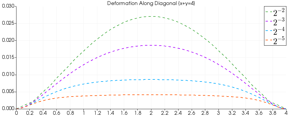
We now explore the geometric behavior of our method. More precisely, it was observed in [5] that there was an artificial displacement along the diagonal , which does not correspond to the actual physics of the problem, namely for . This displacement decreases with smaller mesh size . Our method introduces the same artificial deformation. However, we can see in Figure 1 that this displacement is smaller now, up to one order of magnitude for the last refinement.
6.2. Obstacle Problem
In Example 6.1 we document the flexibility of the dG approach to capture the correct bending behavior of plates. To explore this further, we introduce an extra element to the deformation: a rigid obstacle. We use a square plate clamped on one side and we exert a vertical force. We require that the plate does not penetrate the obstacle. This example is motivated by [7], where the deformation of the plate is the result of thermal actuation of bilayer hinges connected to the plate.
Example 6.2.
Let and be the Dirichlet boundary where we enforce clamped boundary conditions (6.1). We apply the vertical force . We choose a simple case where the obstacle is a rigid flat plate at height . From a mathematical viewpoint, this obstacle problem can be treated by introducing the convex set of admissible deformations
along with splitting of variables. We introduce another deformation , such that always and penalize the -distance between and . If is an obstacle penalty parameter, we add the following extra term to the energy
At the discrete level, this affects the gradient flow at each step, where we use as the -projection of the previous solution in . We refer to [7] for more details about the variable splitting and the projection.
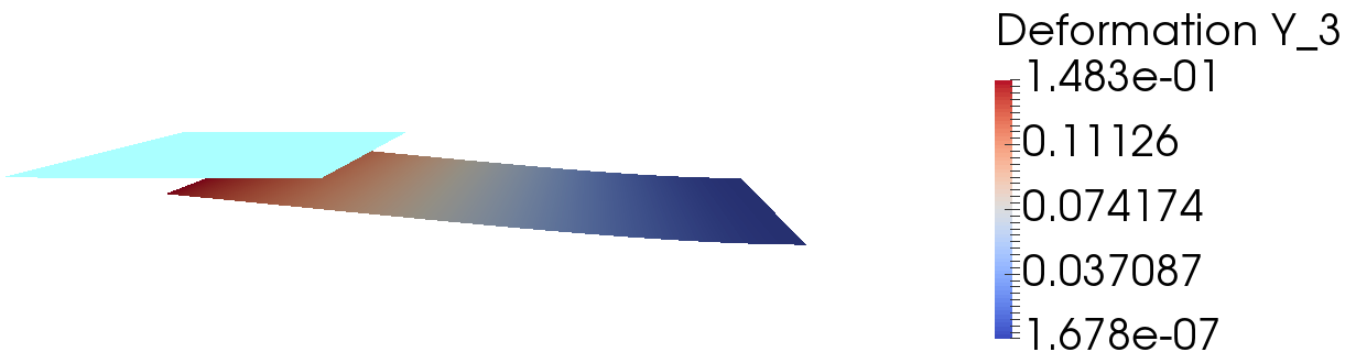
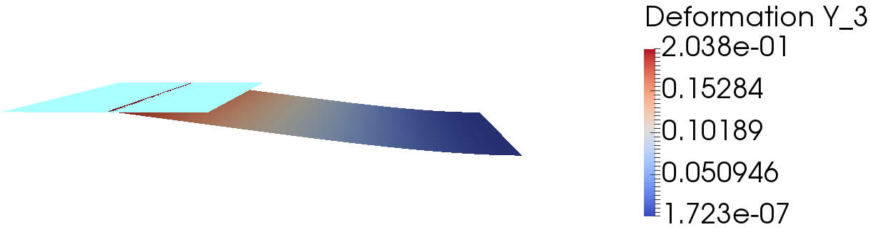
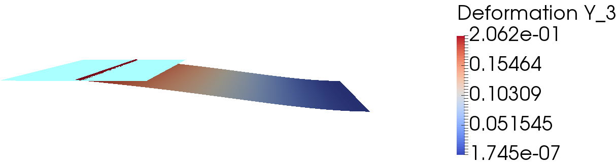
The plate configurations before contact are unaffected by the obstacle presence and dictated by pure bending. Contact occurs with minor penetration of the obstacle because we do not force the deformation to belong to the set , but rather penalize its -distance from its projection to . As time evolves, the plate bends backwards trying to decrease the obstacle crossing because it is energetically costly. This behavior can be enhanced by further mesh refinement and by choosing a smaller obstacle parameter . To illustrate the obstacle-plate interaction, we provide six different steps of the gradient flow in Figure 2. The illustration corresponds to 1024 cells, and time step . The penalty parameters are , and the isometry defect at the end of this simulation is .
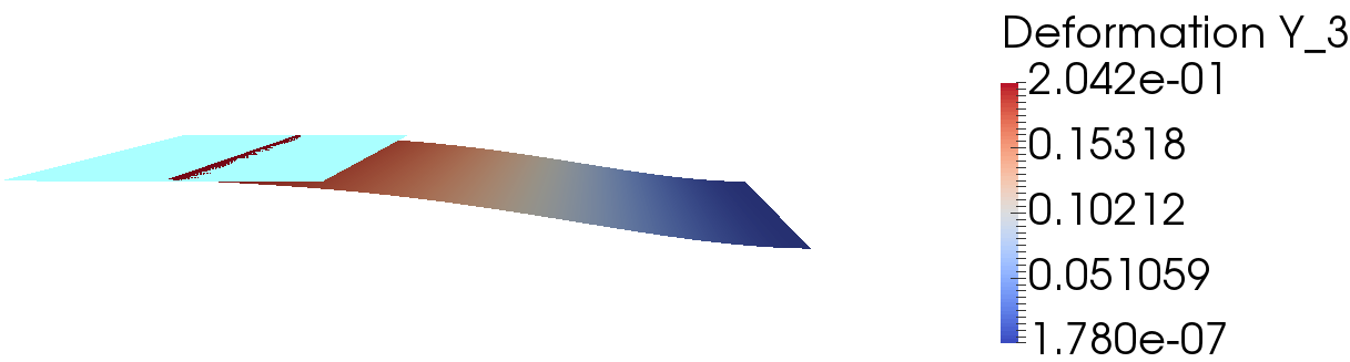
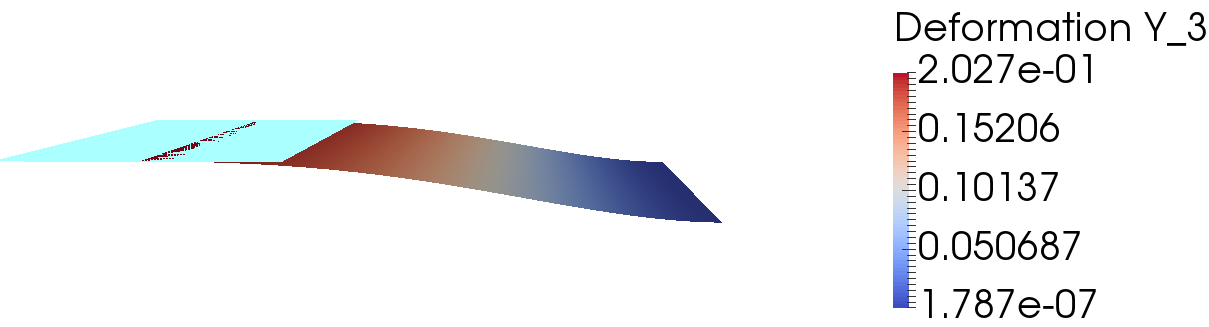
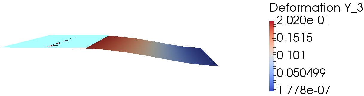
6.3. Compressive Case: Buckling
We finally investigate the geometrically and physically interesting case of buckling. We use a rectangular plate with a small vertical load, that induces a bias for bending, and we impose compressive boundary conditions on two opposite sides. The latter reveals the delicate interplay between the Nitsche’s approach for enforcement of Dirichlet boundary conditions and the choice of suitable initial configurations, for the performance of the gradient flow. This example is also motivated by [5].
Example 6.3.
Let and be the two sides where we impose the compressive boundary conditions
We apply a vertical force of magnitude . Given the compressive nature of the problem, the plate could bend either upwards or downwards (buckling), resulting in two deformations which are the reflection of each other with respect to the plane and have the same minimal energy. This is why we apply a small force upwards to select the deformation with positive third component. Since our initial configuration is flat, there is a boundary mismatch that leads to large boundary penalty terms in the Nitsche’s approach and correspondingly large initial energy . This in turn gives rise to either large isometry defects, because of (3.10) and (3.11), or tiny time steps and very slow evolution. This might explain why we need a stronger force than the one in [5] (i.e. ) because is dominated by the boundary terms. Moreover, to prevent a large from creating very abrupt and non-physical deformations during the gradient flow for moderate , we employ a quasi-static approach: we enforce the boundary conditions gradually thereby avoiding a large mismatch (parameter continuation). We use a parameter that starts from zero and increases throughout the flow until it reaches the value 1. In order to achieve a gradual adjustment to the boundary conditions, we let
and be the Dirichlet boundary conditions for and , where stands for the identity function. As the mesh becomes finer, the growth of parameter must be slower to compensate for the larger initial energy associated with mesh-dependent boundary terms as well as to allow for smooth flow evolutions.
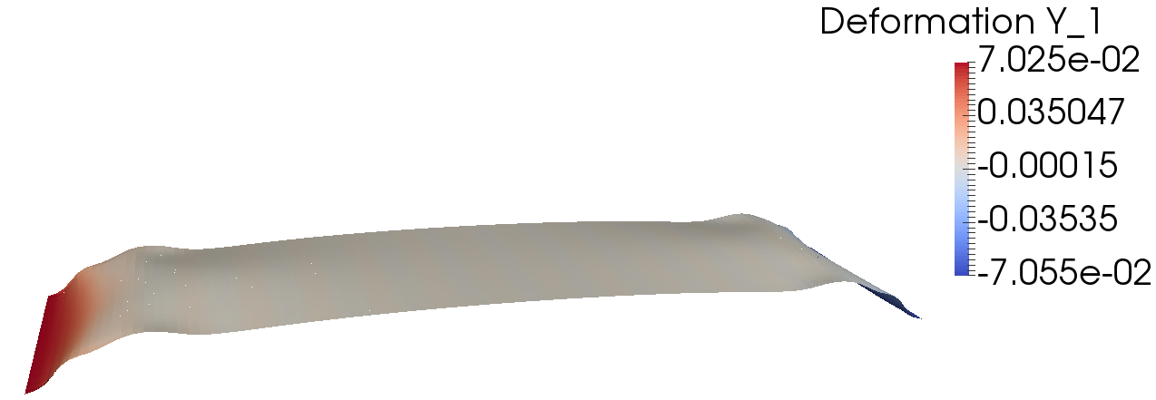

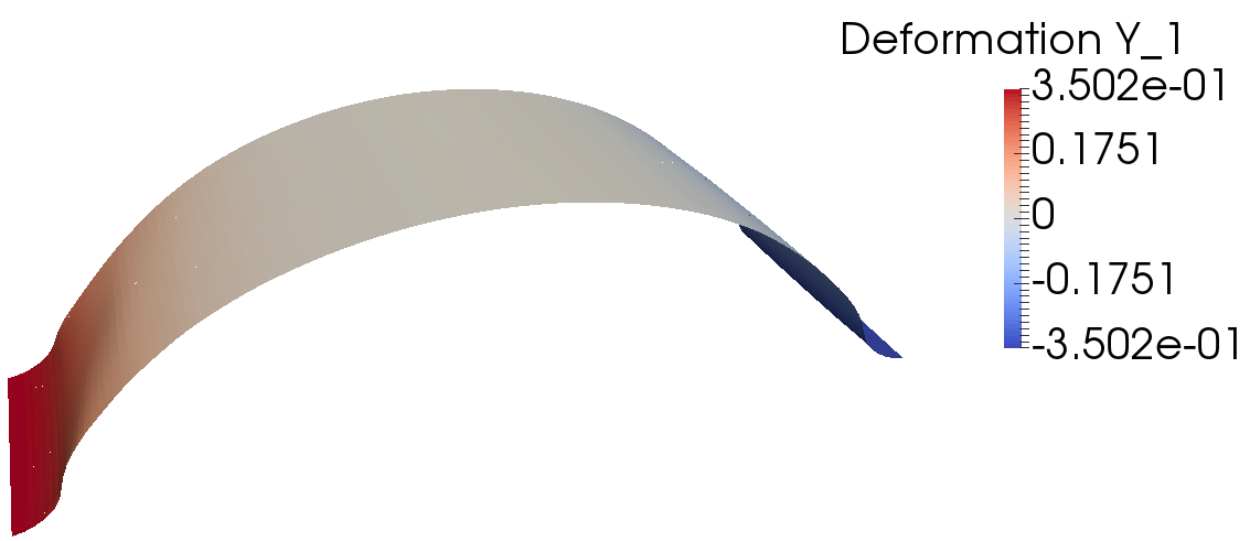
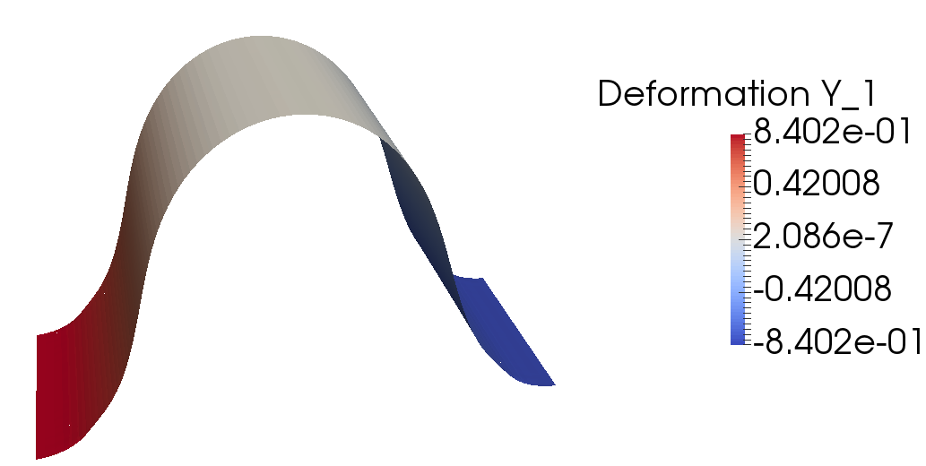
To illustrate the effect of , we depict deformations in Figure 3 that corresponds to various stages of the gradient flow with and time step . The parameter increases linearly by the amount in each iteration. We see that the compressive nature of the boundary conditions becomes more apparent after exceeds the value and that the boundary conditions are attained at the end of the deformation. The final isometry defect is , one order of magnitude smaller than observed in [5].
7. Implementation
We now make some implementation remarks and connect them with the theory in Sections 2 and 3. If are the nodal values of functions , then the matrix form of the saddle point problem (3.7) reads
| (7.1) |
where is the matrix corresponding to the left-hand side of (3.4) and is the matrix associated with (3.6), which depends on . Since does not depend on we can assemble it and perform its LU decomposition once and subsequently use a direct solver whenever we need the action of . For the full system we use the Schur complement approach with a conjugate gradient iterative solver, to first solve for and next recover . The numerical experiments of Section 6 reveal the existence of solution of the discrete gradient flow (3.7), which exhibits small isometry defects asymptotically as grows and confirm the validity of an inf-sup condition for (3.7). However, this issue remains open (see Remark 3.2).
Lastly, it is important to mention that our choice in Section 2 of a space of discontinuous polynomials is strongly motivated by the structure of (7.1). More precisely, if were continuous then the inf-sup condition for in (3.6) would not be local and be harder to achieve. In fact, computational experiments for continuous functions (not reported here) indicate that the conjugate gradient method becomes significantly slower if the functions of are required to be continuous; this justifies our choice of a fully discontinuous space . We refer to [29] for details.
8. Conclusions
In this work we design, analyze and implement a dG approach to construct minimizers for large bending deformations under a nonlinear isometry constraint. The problem is nonconvex and falls within the nonlinear Kirchhoff plate theory. We propose a discrete energy functional and provide a flexible approximation of the isometry constraint. We devise a discrete gradient flow for computing discrete minimizers and enforcing a discrete isometry defect. We construct a discrete approximation of the Hessian inspired by [20, 31] that turns out to be instrumental to prove convergence: convergence of the discrete energy to the continuous one as well as -convergence of global minimizers of the discrete energy to global minimizers of the continuous energy. The existence of the latter is not assumed a-priory, but is rather a consequence of our analysis. Our dG approach simplifies some implementation details and theoretical constructions needed in [5, 8] for the Kirchhoff elements. The dG formulation is also valid for graded isoparametric elements of degree , which is considerably more general than [5, 8]. Moreover, we present numerical experiments that indicate that the dG approach also captures the physics of some problems better than the Kirchhoff approach, while also giving rise to a more accurate approximation of the isometry constraint.
9. Appendix: Estimates for Isoparametric Mappings
In this appendix we present inverse and error estimates involving the Hessian for elements obtained by isoparametric transformations; this includes quadrilaterals mapped by bilinear maps . The issue at stake is that the isoparametric map from the reference element to a generic element is no longer affine but rather belongs to or , whence for . Since the considerations below are local to a single element , we drop the sub-index in . Moreover, we denote by the pullback of a function defined on . Property does not affect the first derivatives of a function but it does influence its higher derivatives. To quantify this effect we recall that we assume that is shape-regular so that and , where the hidden constants depend on shape regularity of . Furthermore, because , Lemma 13.4 in Ern and Guermond[22] (see also Ciarlet and Raviart[19]) guarantees that
| (9.1) |
Our estimates below rely on the following key property of isoparametric maps :
| (9.2) |
If is the Lagrange interpolation operator over of degree and is the corresponding operator induced by the map , then (9.2) translates into
| (9.3) |
If , , then the chain rule gives
| (9.4) | |||
| (9.5) |
This, together with (9.1), yields
| (9.6) | |||
| (9.7) |
This gives relations between the Hessians of and that involve lower order terms. The next two estimates connect higher order derivatives of isoparametric maps.
Lemma 9.1 (inverse estimate).
Let and be an edge of . Then the following estimates are valid for all
| (9.8) |
Proof.
Let be a linear polynomial to be chosen later. Combining (9.4) and (9.1) with an inverse estimate for , according to (9.2), yields
We now map back to using (9.7) for to get
We finally choose as the best linear approximation of in , whence the Bramble-Hilbert lemma yields and gives the first assertion. The remaining assertion follows along the same lines upon differenciating (9.4) once more and using (9.1) with together with the inverse estimate . The proof is complete. ∎
Lemma 9.2 (-stability).
Let for and be the Lagrange interpolant of of degree . The following bound is then valid
| (9.9) |
Proof.
We first note that is well defined because (recall that is closed). In view of (9.3), we see that for any . We utilize (9.6) to deduce
We choose to equal at three vertices of , and observe that vanishes at the corresponding three vertices of and the associated linear Lagrange interpolant vanishes as well. Concatenating an inverse estimate with the interpolation error estimate , valid because , yields
We finally invoke (9.7) to infer that
This leads to the asserted estimate (9.9). ∎
We point out that the usual interpolation estimate
| (9.10) |
with -seminorm on the right-hand side is valid for isoparametric elements with polynomial degree . In fact, transforming to and back to via (9.7) gives
Applying this estimate to , with , and recalling (9.3) leads to (9.10). However, this argument fails for . We now state, and prove for completeness, a key error estimates for quadrilaterals valid for due to Ciarlet and Raviart (see Examples 7 and 8 in [19]). We also refer to (13.27) in Ern and Guermond [22].
Lemma 9.3 (error estimate for quadrilaterals).
Let be so that with bilinear. If and is the Lagrange interpolant of with , then for there holds
| (9.11) |
Proof.
Expression (9.4) in conjunction with (9.1) reveals that mapping from to involves computing all derivatives according to
where stands for all pure derivatives of order . The latter inequality is a consequence of the Bramble-Hilbert estimate for elements; see Theorem 1 in [12]. We now resort to a variant of (9.5) involving derivatives but simplified by the fact that pure derivatives if because is bilinear:
Since , this yields
| (9.12) |
and combined with the previous estimate gives the asserted estimate (9.11). ∎
Lemma 9.3 extends to isoparametric maps for . We quote here Theorem 6 of Ciarlet and Raviart [19]; see also (13.30) in Ern and Guermond [22].
Lemma 9.4 (error estimates for curved quadrilaterals).
Let be so that with and let be the bilinear function that maps the vertices of to those of . Let satisfy
| (9.13) |
If and is the Lagrange interpolant of with , then for there holds
| (9.14) |
References
- [1] D. Arndt, W. Bangerth, D. Davydov, T. Heister, L. Heltai, M. Kronbichler, M. Maier, J.-P. Pelteret, B. Turcksin, D. Wells, The deal.II Library, Version 8.5, Journal of Numerical Mathematics, 25(3):137–146, 2017.
- [2] D. N. Arnold, F. Brezzi, B. Cockburn, L. D. Marini, Unified analysis of discontinuous Galerkin methods for elliptic problems, SIAM J. Numer. Anal., 39(5), 1749–1779, 2002.
- [3] E. Bänsch, P. Morin, R.H. Nochetto, An adaptive Uzawa FEM for the Stokes problem: Convergence without the inf-sup condition, SIAM J. Numer. Anal. 40, 1207–1229, 2002.
- [4] W. Bangerth, R. Hartmann, G. Kanschat, deal.II – a general purpose object oriented finite element library, ACM Trans. Math. Softw., 33(4):24/1–24/27, 2017.
- [5] S. Bartels, Finite element approximation of large bending isometries, Numer. Math. 124, 3, 415-440, 2013.
- [6] S. Bartels, Numerical Methods for Nonlinear Partial Differential Equations, Springer International Publishing, 2015.
- [7] S. Bartels, A. Bonito, Anastasia H. Muliana, R. H. Nochetto, Modeling and simulation of thermally actuated bilayer plates, J. Comp. Phys. 354, 512–528, 2018.
- [8] S. Bartels, A. Bonito, R. H. Nochetto, Bilayer plates: Model reduction, -convergent finite element approximation and discrete gradient flow, Commun. Pure Appl. Math. 70, 3, 547-–589, 2017.
- [9] N. Bassik, B. Abebe, K. Laflin, D. Gracias, Photolithographically patterned smart hydrogel based bilayer actuators, Polymer 51, 6093-6098, 2010.
- [10] K. Bhattacharya, M. Lewicka, M. Schaffner, Plates with incompatible prestrain, Arch. Rational Mech. Anal. 221, 143-–181, 2016.
- [11] A. Bonito, R. H. Nochetto, Quasi-optimal convergence rate of an adaptive discontinuous Galerkin method, SIAM J. Numer. Anal., 48(2), 734-771, 2010.
- [12] J.H. Bramble, S.R. Hilbert, Bounds for a class of linear functionals with applications to Hermite interpolation, Numer. Math., 16, 362–369, 1970/71.
- [13] S. C. Brenner,Poincaré-Friedrichs inequalities for piecewise functions, SIAM J. Numer. Anal., 41(1), 306-324, 2003.
- [14] S. C. Brenner,Two-level additive Schwarz preconditioners for nonconforming finite elements, Math. Comp., 65(215), 897-921, 1996.
- [15] S. C. Brenner, K. Wang, J. Zhao,Poincaré-Friedrichs inequalities for piecewise functions, Numer. Funct. Anal. Optim., 25, 463-478, 2004.
- [16] F. Brezzi, G. Manzini, D. Marini, P. Pietra, A. Russo, Discontinuous Galerkin approximations for elliptic problems, Numer. Methods Partial Differential Equations, 16(4), 365-378, 2000.
- [17] A. Buffa, C. Ortner,Compact embeddings of broken Sobolev spaces and applications, IMA Numer. Anal., 29, 827-855, 2009.
- [18] P. Castillo, B. Cockburn, I. Perugia, D. Schötzau,An a priori error analysis of the local discontinuous Galerkin method for elliptic problems, SIAM J. Numer. Anal., 38, 1676–1706, 2000.
- [19] P.G. Ciarlet, P.-A. Raviart,Interpolation theory over curved elements, with applications to finite element methods, Comput. Methods Appl. Mech. Engrg., 1, 217–249, 1972.
- [20] D. A. Di Pietro, A. Ern, Discrete functional fnalysis tools for discontinuous Galerkin methods with application to the incompressible Navier-Stokes equations, Math. Comp., 79(271), 1303-1330, 2010.
- [21] A. Ern, J-L Guermond, Finite element quasi-interpolation and best approximation, ESAIM: M2AN 51, 1367-1385, 2017.
- [22] A. Ern, J-L Guermond, Finite Elements I: Approximation and interpolation, to appear.
- [23] G. Friesecke, R.D. James, S. Müller, A theorem on geometric rigidity and the derivation of nonlinear plate theory from three-dimensional elasticity, Comm. Pure Appl. Math. 55, 11, 1461-1506, 2002.
- [24] E. Jager, E. Smela, O. Inganäs, Microfabricating conjugated polymer actuators, Science 290, 1540-1545, 2000.
- [25] R.H.W. Hoppe, B. Wohlmuth, Element-oriented and edge-oriented local error estimators for nonconforming finite element methods, RAIRO Modél. Math. Anal. Numér., 30(2), 237-263, 1996.
- [26] P. Hornung, Approximation of flat isometric immersions by smooth ones, Arch. Ration. Mech. Anal. 199, 1015- 1067, 2011.
- [27] J.-N. Kuo, G.-B. Lee, W.-F. Pan, H.-L. Lee, Shape and thermal effects of metal films on stress-induced bending of micromachined bilayer cantilever, Japanese Journal of Applied Physics 44, 5R, 3180, 2005.
- [28] M. Lewicka, P. Ochoa, M.-R. Pakzad, Variational models for prestrained plates with Monge-Ampère constraint, Differential Integral Equations 28, no. 9/10, 861–898, 2015.
- [29] D. Ntogkas, Non-linear geometric PDEs: algorithms, numerical analysis and computation, PhD Thesis, University of Maryland, College Park, 2018.
- [30] P. Oswald, On a BPX-preconditioner for elements, Computing, 51(2), 125-133, 1993.
- [31] T. Pryer, Discontinuous Galerkin methods for the biharmonic equation from a discrete variational perspective, Electronic Transactions of Numerical Analysis, 2014.
- [32] B. Rivière, Discontinuous Galerkin Methods for Solving Elliptic and Parabolic Equations: Theory and Implementation, Society for Industrial and Applied Mathematics, 2008.
- [33] O. Schmidt, K. Eberl, Thin solid films roll up into nanotubes, Nature 410, 168, 2001.
- [34] E. Smela, O. Inganös, I. Lundström, Controlled folding of micrometer-size structures, Science 268, 5218, 1735–1738, 1995.