Group Fairness in Bandits with Biased Feedback

Abstract.

We propose a novel formulation of group fairness with biased feedback in the contextual multi-armed bandit (CMAB) setting. In the CMAB setting, a sequential decision maker must, at each time step, choose an arm to pull from a finite set of arms after observing some context for each of the potential arm pulls. In our model, arms are partitioned into two or more sensitive groups based on some protected feature(s) (e.g., age, race, or socio-economic status). Initial rewards received from pulling an arm may be distorted due to some unknown societal or measurement bias. We assume that in reality these groups are equal despite the biased feedback received by the agent. To alleviate this, we learn a societal bias term which can be used to both find the source of bias and to potentially fix the problem outside of the algorithm. We provide a novel algorithm that can accommodate this notion of fairness for an arbitrary number of groups, and provide a theoretical bound on the regret for our algorithm. We validate our algorithm using synthetic data and two real-world datasets for intervention settings wherein we want to allocate resources fairly across groups.

Knowing that one may be subject to bias is one thing; being able to correct it is another.

Jon Elster

1. Introduction

In many online settings, a computational or human agent must sequentially select an item from a slate, receive feedback on that selection, and then use that feedback to learn how to select the best items in the following rounds. Within computer science, economics, and operations research circles, this is typically modeled as a multi-armed bandit (MAB) problem Sutton and Barto (2017). Examples include algorithms for selecting what advertisements to display to users on a webpage Mary et al. (2015), systems for dynamic pricing Misra et al. (2019), and content recommendation services Li et al. (2010). Indeed, such decision-making systems continue to expand in scope, making ever more important decisions in our lives such as setting bail Corbett-Davies and Goel (2018), making hiring decisions Bogen (2019); Schumann et al. (2019a), and policing Rudin (2013). Thus, the study of the properties of these algorithms is of paramount importance as highlighted by Chouldechova and Roth (2018) motivating priorities for fairness research in machine learning.

In the basic MAB setting, there are $n$ arms, each associated with a fixed but unknown reward probability distribution Lai and Robbins (1985); Auer et al. (2002). At each time step $t\in T$, an agent pulls an arm and receives a reward that is independent of any previous action and follows the selected arm’s probability distribution. The goal of the agent is to maximize the total collected reward over time. A generalization of MAB is the contextual multi-armed bandit (CMAB) where the agent observes a $d$-dimensional context along with the observed rewards to choose a new arm. In the CMAB problem, the agent learns the relationship between contexts and rewards and selects the best arm Agrawal and Goyal (2013).

Yet, the use of MAB- and CMAB-based systems often results in behavior that is societally repugnant. Sweeney (2013a) noted that queries for public records on Google resulted in different contextual advertisements based on whether the query target had a traditionally African American or Caucasian name; in the former case advertisements were more likely to contain text relating to criminal incidents. Following that initial report similar instances continue to be observed, both in the bandit setting and in the general machine learning world O’Neil (2016). In lockstep, the academic community has begun developing approaches to tackling issues of (un)fairness in learning settings. We have an opportunity to identify and understand why the data we have may be causing the bias.

A Computing Community Consortium (CCC) report on fairness in ML identified that most studies of fairness are focused on classification problems Chouldechova and Roth (2018). These works define a statistical notion of fairness, typically a notion of equal treatment of equals Rawls (1971), and propose algorithms to abide by these constraints. Two issues identified by Chouldechova and Roth (2018) that we address in this paper are extensions to notions of group fairness and looking at fairness in online dynamic systems, e.g., CMABs. We address these gaps by formalizing and providing an algorithm for fairness with biased feedback when the arms of the bandit can be partitioned into groups. Direct applications of our work including scenarios discussed within the AAMAS community like aiding the allocation of human resources in talent sourcing Schumann et al. (2020).

The recent AI100 study Littman et al. (2021), whose goal is to take a broad and long term look at the opportunities and pitfalls for AI researchers, has highlighted the need to develop systems that work with humans, providing oversight, transparency, and explanation. Our bandit formulation is one step towards creating more human-centered AI Shneiderman (2020a), a new area of study that seeks to understand and balance computer automation and autonomy with the level of human control in a given system. Many of the negative applications of MAB based systems we have discussed so far too often occur because there is too much autonomy given to the system, and it optimizes away from what humans or society considers desirable. By explicitly modeling the underlying bias term, we hope to improve computer aided decision making by understanding and mitigating the dangers that can occur when there are excessive levels of human control or excessive levels of computer autonomy; leading to systems that are more transparent, auditable, and trustworthy.

Running Example. As a running example throughout the paper, imagine the position of an agent at a bank or a lender on a micro-lending site. Here, the agent must sequentially pick loans to fund. In many cases, such as the micro-lending site Kiva, a user is presented with a slate of potential loans they may fund when they log in and this slate is generated by a recommender system Sonboli et al. (2020). Each of these loans, i.e. arms, has a context which includes attributes of the applicant (e.g., personal statement, repayment history, business plan). The loans can also be partitioned into sets of $m$ sensitive attributes, e.g. location, race, or gender. In the simplest case, assume we have two female applicants and two male applicants on the slate at a given time. We also assume that when pulling an arm from, for example, a female applicant, there is some societal bias introduced into the reward. Yet, in many settings (and, as we assume in this work), the average true (i.e., unbiased) reward across groups is equal. We want to balance the number of times the agent selects women versus men given this societal bias built into the feedback.

While we use loans as our running example, our notion of regret could be extended to a number of other areas including recent work in MAB problems on hiring situations Schumann et al. (2019b), including the recent AAMAS Blue Sky Paper by Schumann et al. (2020) specifically calling for the community to contribute to fair hiring. One could imagine a situation where hiring decisions are made w.r.t. a short-term reward signal that is biased, versus a longer-term reward of performance which is less biased, e.g., via an end-of-year review that is based on a more quantitative metric such as on-the-job performance. A similar argument can be made about school admissions or matching workers to online tasks in a crowdwork setting.

Contributions.

We propose a novel formulation of group fairness in the contextual multi-armed bandit (CMAB) setting. In our model, arms are partitioned into two or more sensitive groups based on some protected feature, e.g., race. Despite the fact that there may be differences in expected payout between the groups, we may wish to ensure some form of fairness between picking arms from the various groups. Our goal is to capture the phenomena where we want to balance the arms being pulled from both groups and (learn to) ignore societal bias generated by sensitive group membership. We define two novel notions of reward and regret to capture implicit societal bias: proportional parity and equal group parity. We provide a novel algorithm that can accommodate these notions of fairness for an arbitrary number of groups, learn the societal bias term itself, and provide bounds on the regret for our algorithm. We validate our algorithms using synthetic data and real-world datasets for intervention settings wherein we want to allocate resources fairly across protected groups.

2. Related Work

Fairness in machine learning has become one of the most active topics in computer science Chouldechova and Roth (2018). The idea of using formal notions of fairness, i.e. axioms or properties, to design decision schemes has a long history in economics and political economy Rawls (1971); Young (1995). Typically within ML research, fairness is operationalized using the Rawlsian idea that similar individuals should be treated similarly; formally extended to the classification setting by Dwork et al. (2012), who provided algorithms to ensure individual fairness at the cost of the utility of the overall system. Their work underscores that in many cases statistical parity is not sufficient to ensure individual fairness, as we may treat groups fairly but in doing so may be very unfair to some specific individual. Determining when, how, and if to define fairness is an ongoing discussion with roots well before the time of computer science Smith (1776); indeed, it is known that many natural conditions for fairness cannot be achieved in tandem Kleinberg et al. (2016). Still, group fairness is found in many fielded systems Wexler et al. (2019); Bellamy et al. (2019), and we focus on it here.

The study of fairness in MAB was initiated by Joseph et al. (2016a), who showed for both MAB and CMAB one can implement a fairness definition where within a given pool of applicants, e.g., college admission or mortgages, a worse applicant is not favored over a better one, despite a learning algorithm’s uncertainty over the true payoffs. However, Joseph et al. (2016a) only focus on individual fairness, and do not formally treat the idea of group fairness. Individual fairness is, in some sense, group fairness taken to an extreme, where every arm is its own singleton group; it offers strong guarantees, but under strong assumptions Kearns et al. (2018); Binns (2020).

Celis et al. (2019) propose a bandit-based approach to personalization where arm pulls are constrained to fit some probability distribution defined by a fairness metric such as demographic parity. For example, when recommending news articles, their algorithm provides personalized articles from both left and right sources. Their formulation is perhaps closest in the literature to our formulation as it deals with group fairness, however it does not explicitly assume biased feedback. Instead, it enforces a fair probability distribution without learning about the bias present in the data.

There are a number of other recent studies of fairness in the MAB literature. Chen et al. (2020) investigate a task allocation setting with a fairness constraint that captures a minimum rate at which a task is assigned to a particular arm; their model is quite general and captures the adversarial and some non-stationary settings. Liu et al. (2017) look at fairness between arms under the assumption that arm reward distributions are similar (another interpretation of equal treatment of equals). Patil et al. (2019) define fairness such that each arm must be pulled for a predetermined required fraction over the total available rounds. Claure et al. (2019) use the MAB framework to distribute resources amongst teammates in human-robot interaction settings; again, fairness is defined as a pre-configured minimum rate that each arm must be pulled. Hossain et al. (2021) take a more theory-oriented approach to a similar setting, proposing a multi-agent varient of a stochastic MAB setting with a Nash social welfare definition of fairness.

Since preliminary versions of this work were presented Schumann et al. (2020, 2019c) there have been several papers that have investigated similar problems. Wang et al. (2021) look at fairness of exposure in CMAB base systems, specifically focusing on similarity of merit, which is more in line with individual rather than the group fairness we consider here. Tang et al. (2021) consider a setting inspired by liver transplantation where the objective is to trade off a more egalitarian, max-min, policy in allocating opportunities for surgeons to gain experience in liver transplant training. Finally, Ron et al. (2021) investigate a setting of allocating opportunities to sub-populations in a corporate decision making setting where each arm needs to pulled at least a budgeted number of times, but where the cost of allocating an opportunity to a non-optimal arm is known in advance. Interestingly, their algorithmt also achieves a $T^{2/3}$ regret, similar to our results.

One needs to be careful when appealing to purely statistical metrics for ensuring fairness. As argued by Corbett-Davies and Goel (2018), simply setting our sights on a form of classification parity, i.e., forcing that some statistical measure be normalized across groups, we may miss bigger picture issues. Specifically, by only focusing on the statistics of the data we have, we miss an opportunity to identify and understand why the data we have may be causing the bias. Later, we will argue that our novel formalization of regret allows us to actually learn particular sources of bias that may exist in our data.

3. Preliminaries

We follow the standard CMAB setting and assume that we are attempting to maximize a measure over a series of time steps $t\in T$. We assume that there is a $d$-dimensional domain for the context space, $\mathcal{X}=\mathbb{R}^{d}$. The agent is presented with a set $A$ of arms from which to select and we have $|A|=n$ total arms. Each of these arms is associated with a, possibly disjoint, context space $\mathcal{X}_{i}\subseteq\mathcal{X}$. Additionally, we assume that we have $m$ sensitive groups and that the arms are partitioned into these sensitive groups such that $P_{1}\cap\cdots\cap P_{m}=\emptyset$, $P_{1}\cup\cdots\cup P_{m}=A$, and $\forall_{i\in m}|P_{i}|>1$. For exposition’s sake, we assume a binary sensitive attribute with $m=2$ for the remaining of the paper. However, we show the generality of our results to any number of groups in Section 4.

Each arm $i$ has a true linear reward function $f_{i}:\mathcal{X}\rightarrow\mathbb{R}$ such that $f_{i}(x)=\beta_{i}\cdot x$ where $\beta_{i}$ is a vector of coefficients that is unknown to the agent. During each round $t\in T$, a context $x_{t,i}\in\mathcal{X}_{i}$ is given for each arm $i$. One arm is pulled per round. When arm $i$ is pulled during round $t$, a reward is returned: $r_{t,i}=f_{i}(x_{t,i})+e_{t,i}$ where $e_{t,i}\sim\mathcal{N}(0,1)$. The goal of the agent is to minimize the regret over all timesteps in $T$. Formally, the regret of the agent at timestep $t$ is the difference between the arm selected and the best arm that could have been selected. Let $i^{*}$ denote the optimal arm that could be selected and $a$ be the selected arm. Then, the regret at $T$ is

$$R(T)=\sum_{t=1}^{T}f(x_{i^{*},t})-f(x_{a,t}).$$ (1)

In this paper we compare our proposed algorithm against three other algorithms: TopInterval, a variation of LinUCB from Li et al. (2010) with additional annotations to track group membership and treatment of arms, NaiveFair which randomly picks a sensitive group and then applies TopInterval to that group, and IntervalChaining, an individually fair algorithm from Joseph et al. (2016b). All algorithms use ordinary least squares (OLS) estimators of the arm coefficients $\hat{\beta}_{i}$ with a confidence variable $w_{i,t}$ such that the true utility lies within $[\hat{\beta}_{i}\cdot x_{i,t}-w_{i,t},\hat{\beta}_{i}\cdot x_{i,t}+w_{i,t}]$ with probability $1-\delta$. NaiveFair implements a naive version of demographic parity without explicitly looking at societal bias. TopInterval either explores by pulling an arm uniformly at random or exploits by pulling the arm with the highest upper confidence $\hat{\beta}_{i}\cdot x_{i,t}+w_{i,t}$. To ensure individual fairness, IntervalChaining either explores by choosing an arm uniformly at random or exploits by pulling arms that have overlapping confidence intervals with the arm with the highest upper confidence.

3.1. Regret with Societal Bias

As mentioned before, ground truth rewards for sensitive groups can be noisy due to societal or measurement bias. We now formalize this bias in terms of multi-armed bandits. For ease of exposition we assume two groups, but we generalize this in our results. Again, we assume that $n$ arms can be partitioned into two sets $P_{1}$ and $P_{2}$ such that $P_{1}\cap P_{2}=\emptyset$ and $P_{1}\cup P_{2}=[n]$. We consider $P_{1}$, with $|P_{1}|>1$ as the sensitive set, or set with some societal bias. In this situation, each arm $i$ has another true utility function $f^{*}(x_{i,t})=\beta_{i}\cdot x_{i,t}$ where $\beta_{i}$ is a vector of coefficients; if arm $i$ is pulled at timestep $t$ the following reward is returned:

$$r_{i,t}=\beta_{i}\cdot x_{i,t}+\mathbbm{1}[i\in P_{1}]\psi_{P_{1}}\cdot x_{i,t}+\mathcal{N}(0,1),$$ (2)

where $\mathbbm{1}[i\in P_{1}]=1$ when $i\in P_{1}$ and 0 otherwise, and $\psi_{P_{1}}$ is a societal or systematic bias against group $P_{1}$. Note that $\psi_{P_{2}}$ is a zero vector for the non-sensitive group. Hence, the underlying biased utility function can be written as $f(x_{i,t})=\beta_{i}\cdot x_{i,t}+\mathbbm{1}[i\in P_{1}]\psi_{P_{1}}\cdot x_{i,t}$.

Using our running example, let’s assume that the down payment reward received has some bias against the male applicants compared to the female applicants, while the final repayment does not. Note that the final repayment is not measured after accepting a loan and is only measured much later. The loan agency should then take the bias into account while learning what ‘good’ applications look like. Or, in a hiring setting, an applicant may have a biased interview (initial reward) while their true performance is measured only after working for a year (later true reward).

We define true regret for pulling an arm $a$ at time $T$ as

$$R^{*}(T)=\sum_{t=1}^{T}f^{*}(x_{i^{*},t})-f^{*}(x_{a,t})$$ (3)

where $i^{*}$ is the optimal arm to pull at timestep $t$ and $f^{*}(x_{i,t})$ is the true reward with no bias terms $\psi_{P_{1}}\cdot x_{i,t}$. We also assume that the average true reward (with no bias) for group $P_{1}$ should be the same as the average reward for group $P_{2}$. Compare this to Equation 1, which would return the regret on the biased reward function $f(x_{i,t})$. In the loan agency example, this real regret $f^{*}(x_{i,t})$ would measure the regret of the final repayments instead of the biased down payment regret.

One can view the societal bias term $\psi_{i}$ that we learn for some group $i$ as our algorithm learning how to automatically identify and adjust for anti-discrimination for group $i$ compared to all other groups. Anti-discrimination is the practice of identifying a relevant feature in data and adjusting it to provide fairness under that measure Corbett-Davies and Goel (2018). One example of this, discussed by Dwork et al. (2012), Joseph et al. (2016a), and in the official White House algorithmic decision making statement of the President et al. (2016), comes up in college admissions. Given other factors, specifically income level, some colleges weight SAT scores less in wealthy populations due to the presence of tutors while increasing the weight of working-class populations Belkin (2019). While in these admissions settings the adjustments may be ad-hoc, we learn our bias term from data. Past work has compared the vector $\beta$ learned for each arm as akin to adjusting for these biases Dwork et al. (2012). While this is true at an individual level, our explicit modeling of bias allows us to discover these adjustments at a group level.

4. Group Fair Contextual Bandits

In this section, given our new definition of reward (Equation 2) and corresponding new definition of regret (Equation 3), we present the algorithm GroupFairTopInterval (Algorithm 1) which takes societal bias into account. We also give a bound on its regret in this new reward and regret setting. Subsequently, we briefly describe the algorithm.

In GroupFairTopInterval, each round $t$ is randomly chosen with probability $\frac{1}{t^{1/3}}$ to be an exploration round. The exploration round randomly chooses an arm to pull.

The remaining rounds become exploitation rounds, where linear estimates are used to pull arms. GroupFairTopInterval learns two different types of standard OLS linear estimators Kuan (2004). The first is a coefficient vector $\hat{\beta}_{i,t}$ for each arm $i$ (line 7). Additionally, GroupFairTopInterval learns a group coefficient vector $\hat{\psi}_{P_{j},t}$ for each group $P_{j}$ (lines 4 and 5). To calculate these coefficient vectors, the algorithm keeps track of previous arm pull rewards for each arm $i$ at every timestep $t$ in a vector $Y_{i,t}$, and the corresponding contexts for each arm pull in a matrix $X_{i,t}$. A similar vector $\mathcal{Y}_{P_{j},t}$ and matrix $\mathcal{X}_{P_{j},t}$ is kept for both groups $P_{j}$. As mentioned previously, we treat $P_{1}$ as the sensitive group of arms. An arm $i$ in the non-sensitive group $P_{2}$ has a reward estimation of $\hat{\beta}_{i,t}\cdot x_{i,t}$, while an arm $i$ in the sensitive group $P_{1}$ has a bias corrected reward estimation of $\hat{\beta}_{i,t}\cdot x_{i,t}-\hat{\psi}_{P_{1},t}+\hat{\psi}_{P_{2},t}$.

For each arm $i$, the algorithm calculates confidence intervals $w_{i,t}$ around the linear estimates $\hat{\beta}_{i,t}\cdot x_{i,t}$ using a Quantile function $Q$ (line 9). This means that the true utility (including some bias) falls within $[\hat{\beta}_{i,t}\cdot x_{i,t}-w_{i},\hat{\beta}_{i,t}\cdot x_{i,t}+w_{i}]$ with probability $1-\delta$ at every arm $i$ and every timestep $t$. Similarly, for each group $P_{j}$ and context $w_{i,t}$ for a given arm $i$ at timestep $t$, the algorithm calculates a confidence interval $b_{P_{j},i,t}$ using a Quantile function $Q$ (lines 4 and 5). This means that the true group utility (or true average group utility) falls within $[\hat{\psi}_{P_{j},i,t}\cdot x_{i,t}-b_{P_{j},i,t},\hat{\psi}_{P_{j},i,t}\cdot x_{i,t}+b_{P_{j},i,t}]$ with probability $[1-\delta]$. Using the confidence intervals $w_{i,t}$ and $b_{P_{j},i,t}$, and the linear estimates $\hat{\beta}_{i,t}\cdot x_{i,t}$ and $\hat{\psi}_{P_{j},i,t}\cdot x_{i,t}$, we calculate the upper bound of the estimated reward for each arm $i$ (lines 15 and 17), pulling the arm with the highest upper bound (line 18).

Algorithm 1 GroupFairTopInterval

0:  $\delta$, $P_{1}$, $P_{2}$

1:  for $t=1\ldots T$ do

2:     With probability $\frac{1}{t^{1/3}}$, play $i_{t}\in_{R}\{1,\ldots,n\}$ and observe reward $y_{i_{t},t}$

3:     otherwise:

4:        $\hat{\psi}_{P_{1},t}\vcentcolon=\left(\mathcal{X}_{P_{1},t}^{T}\mathcal{X}_{P_{1},t}\right)^{-1}\mathcal{X}_{P_{1},t}^{T}\mathcal{Y}_{P_{1},t-1}$

5:        $\hat{\psi}_{P_{2},t}\vcentcolon=\left(\mathcal{X}_{P_{2},t}^{T}\mathcal{X}_{P_{2},t}\right)^{-1}\mathcal{X}_{P_{2},t}^{T}\mathcal{Y}_{P_{2},t-1}$

6:        for $i=1\ldots n$ do

7:           $\hat{\beta}_{i,t}\vcentcolon=\left(X_{i,t}^{T}X_{i,t}\right)^{-1}X_{i,t}^{T}Y_{i,t-1}^{T}$

8:           $F_{i,t}\vcentcolon=\mathcal{N}\left(0,\sigma^{2}x_{i,t}\left(X_{i,t}^{T}X_{i,t}\right)^{-1}x_{i,t}^{T}\right)$

9:           $w_{i,t}\vcentcolon=Q_{F_{i,t}}\left(\frac{\delta}{2nt}\right)$

10:           if $i\in P_{1}$ then

11:              $\mathcal{F}_{P_{1},i,t}\vcentcolon=\mathcal{N}\left(0,\sigma^{2}x_{i,t}\left(\mathcal{X}_{P_{1},t}^{T}\mathcal{X}_{P_{1},t}\right)x_{i,t}^{T}\right)$

12:              $\mathcal{F}_{P_{2},i,t}\vcentcolon=\mathcal{N}\left(0,\sigma^{2}x_{i,t}\left(\mathcal{X}_{P_{2},t}^{T}\mathcal{X}_{P_{2},t}\right)x_{i,t}^{T}\right)$

13:              $b_{P_{1},i,t}\vcentcolon=Q_{\mathcal{F}_{P_{1},i,t}}\left(\frac{\delta}{2\frac{n}{|P_{1}|}T}\right)$

14:              $b_{P_{2},i,t}\vcentcolon=Q_{\mathcal{F}_{P_{2},i,t}}\left(\frac{\delta}{2\frac{n}{|P_{2}|}T}\right)$

15:              $\hat{u}_{i,t}\vcentcolon=\hat{\beta}_{i,t}\cdot x_{i,t}+w_{i,t}-\hat{\psi}_{P_{1},t}\cdot x_{i,t}+b_{P_{1},i,t}+\hat{\psi}_{P_{2},t}\cdot x_{i,t}+b_{P_{2},i,t}$

16:           else

17:              $\hat{u}_{i,t}\vcentcolon=\hat{\beta}_{i,t}\cdot x_{i,t}+w_{i,t}$

18:        Play $\operatorname*{\arg\!\max}_{i}\hat{u}_{i,t}$ and observe reward $y_{i,t}$

Returning to our running example, using GroupFairTopInterval, the loan agency would learn a down payment reward function for each of the arms, i.e., a coefficient vector $\beta_{i}$ where $i\in[$young female arm, young male arm, older female arm, older male arm$]$, as well as the group average coefficients for the gender-grouped arms, $\psi_{P_{j}}$, for male and female. Using the gender-grouped coefficients, expected rewards for male arms are reweighted to account for the bias in down payment.

Standard algorithms like TopInterval would choose an arm $i=\operatorname*{\arg\!\max}(\hat{\beta}\cdot x_{i,t}+w_{i,t})$, ignoring societal bias (Equation 2, leading to a larger true regret (Equation 3)). Note that GroupFairTopInterval can be extended to multiple groups by defining an overall average reward.

GroupFairTopInterval is fair—in the context of our group fairness definitions—and satisfies the following theorem. Appendix B of the full paper provides a detailed, complete proof.

Theorem 1.

For two groups $P_{1}$ and $P_{2}$, where $P_{1}$ has a bias offset in rewards, GroupFairTopInterval has regret

Proof Sketch.

We start by proving two lemmas. The first of which states that with probability at least $1-\delta$:

$$\left|\hat{\beta}_{i,t}\cdot x_{i,t}-(\beta_{i}\cdot x_{i,t}+\mathbbm{1}[i\in P_{1}]\psi_{P_{1}}\cdot x_{i,t})\right|\leq w_{i,t}$$ (4)

holds for any $i$ at time $t$. Similarly, the second states that with probability at last $1-\delta$:

$$\left|\hat{\beta}_{i,t}\cdot x_{i,t}-\beta_{i}\cdot x_{i,t}\right|\leq w_{i,t}$$ (5)

holds for any group $P_{j}$, any arm $i$, and at any timestep $t$. By combining these two lemmas, we can see that arms should be treated fairly.

The regret for GroupFairTopInterval can be broken down into three terms:

$$R^{*}(T) =\sum_{t:\ t\textit{ is an explore round}}\mathit{regret}(t)$$ (6)

$$+\sum_{t:\ t\textit{ is an exploit round and }t<T_{1}}\mathit{regret}(t)$$

$$+\sum_{t:\ t\textit{ is an exploit round and }t\geq T_{1}}\mathit{regret}(t).$$ (7)

First, for any $t$ we have:

$$\sum_{t^{\prime}<t}\frac{1}{t^{1/3}}=\Theta(t^{2/3}).$$ (8)

We then show that the number of rounds $T_{1}$ after which we have sufficient samples such that the estimators are well concentrated is:

$$T_{1}=\Theta\left(\min_{a}\left(\frac{dnL}{\lambda_{min_{a,d}}}\left(\ln^{2}\frac{2}{\delta}+\ln d\right)\right)^{3/2}\right).$$ (9)

Finally, we bound the third term in Equation 6 as follows:

$$\sum_{t:\ t\textit{ is an exploit round and }t\geq T_{1}}regret(t)$$ (10)

$$\leq O\left(\sqrt{dn\frac{\ln\frac{2nT}{\delta}}{\min_{i}\lambda_{\min_{i,d}}}}T^{2/3}+\delta^{\prime}T\right).$$ (11)

Combining Equations 6, 8, 9, and 10, we have Theorem 1. ∎

Note that we can extend Algorithm 1 to $m$ groups. In this setting, we make the strong assumption that true rewards are centered about $\rho$ defined by the user. In this adaption of the algorithm, we set the upper bound radius for arm $i$ as:

$$\hat{u}_{i,t}=\hat{\beta}_{i,t}\cdot x_{i,t}+w_{i,t}+\rho-\hat{\psi}_{P_{j},t}\cdot x_{i,t}+b_{P_{j},i,t}$$

where $i\in P_{j}$. We then have the following theorem for multiple groups:

Theorem 2.

For $m$ groups $P_{1},\ldots,P_{m}$, GroupFairTopInterval (Multiple Groups) has regret

where $l=\min_{i}\lambda_{min_{i,d}}$, with $\lambda_{min_{i,d}}$ the smallest eigenvalue of $X_{i,t}^{T}X_{i,t}$; and $L>\max_{t}\lambda_{\max}(x_{i,t}^{T}x_{i,t})$.

5. Experiments

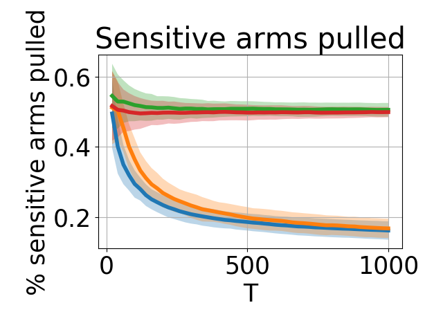
(a) Increasing the total budget $T$, for $n=10$, $\mu=10$, and number of sensitive arms = $5$

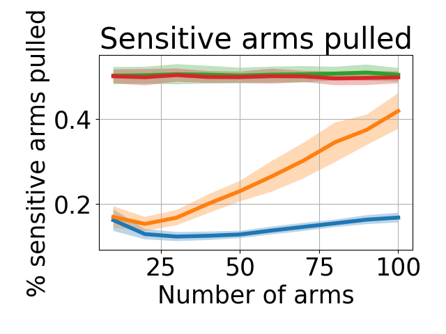
(b) Increasing the number of arms $n$, for $T=1000$, $\mu=10$, and number of sensitive arms = $5$

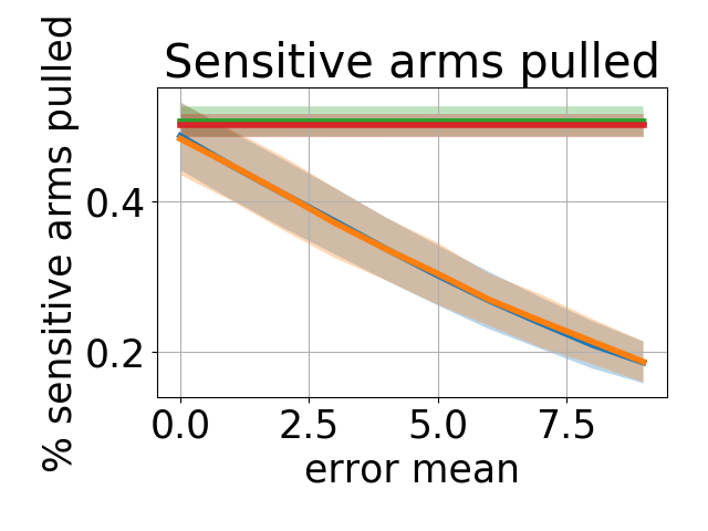
(c) Increasing $\mu$, for $n=10$, $T=1000$, and number of sensitive arms = $5$

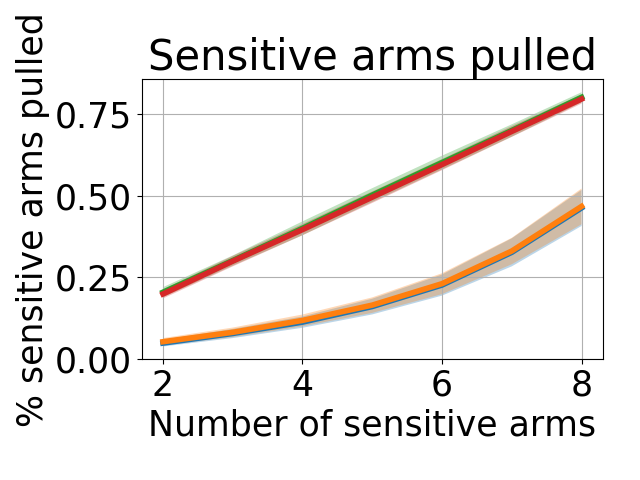
(d) Increasing the fraction of overall sensitive arms, for $n=10$, $T=1000$, $\mu=10$

(e) Legend

Figure 1. Percentage of total arm pulls that were pulled using sensitive arms.

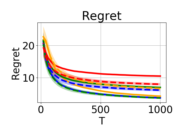
(a) $n=10$, $\mu=10$, # of sensitive arms = 5

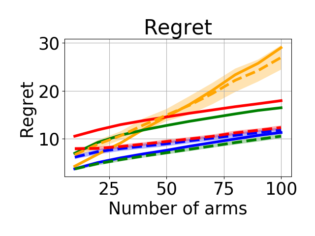
(b) $T=1000$, $\mu=10$, # of sensitive arms = 5

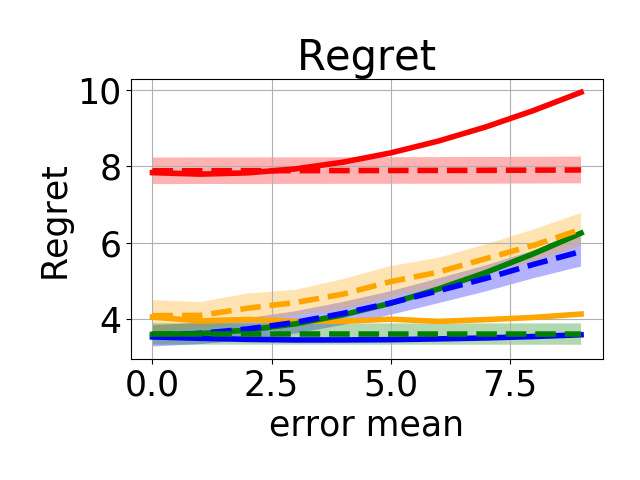
(c) $n=10$, $T=1000$, # of sensitive arms = 5

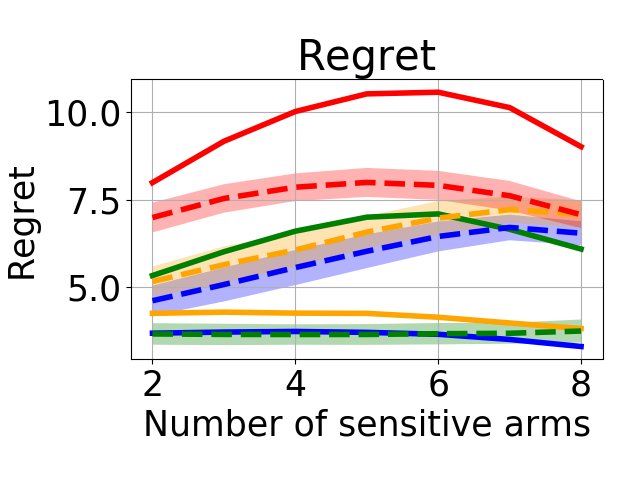
(d) $n=10$, $T=1000$, $\mu=10$

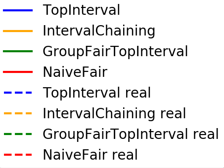
(e) Legend

Figure 2. Regret for synthetic experiments. The solid lines are regret given the rewards received from pulling the arms (including the group bias). The dashed lines is the true regret (without the group bias).

To empirically evaluate GroupFairTopInterval, we perform experiments on synthetic data to demonstrate the effects of various parameters, and on real datasets to demonstrate how GroupFairTopInterval performs in the wild. In each of these sections we compare to TopInterval, due to Li et al. (2010), NaiveFair (See Section 5.1), and IntervalChaining, due to Joseph et al. (2016a).

5.1. NaiveFair

One popular definition of group fairness in classification is the notion of demographic parity. Formally, given a protected demographic group $A$, we want:

$$\Pr(\hat{Y}=1|A=0)=\Pr(\hat{Y}=1|A=1),$$ (12)

where the probability of assigning a classification label $\hat{Y}=1$ does not change based on the sensitive attribute class $A$. Demographic parity is important when ground truth classes $Y$ are extremely noisy for sensitive groups due to some societal or measurement bias. Assume that we have a classifier that predicts whether an individual should receive a loan where our sensitive attribute $A$ is binary gender. Demographic parity states that the probability of getting a loan should be the same for males ($A=0$) and females ($A=1$).

In converting this definition of demographic parity to the the multi-armed bandit setting, we alter the definition to be that the probability of pulling an arm $a$ does not change based on group membership $P_{j}$:

$$\Pr(\textit{pull }a|a\in P_{0})=\Pr(\textit{pull }a|a\in P_{1}).$$ (13)

Continuing our running example, assume we are a loan agency. The loan agency receives 4 applications at every timestep $t$: an applicant from a young female, an applicant from a young male, an applicant from a older female, an applicant from an older male; we must choose one application to grant at each timestep. After granting a loan the loan agency receives a down payment on that loan as reward. This reward is then used to update the estimates of whether or not a “good” loan application was received for the pulled arm. Assume that the loan agency wants to act fairly using the binary sensitive attribute of gender. Then, the probability that the loan agency chooses a female applicant at timestep $t$ should be the same as the probability of choosing a male applicant.

Algorithm 2 NaiveGroupFair

0:  $\delta$, $P_{1}$, $P_{2}$

1:  for $t=1\ldots T$ do

2:     $P\leftarrow$ Randomly choose group $P_{1}$ or $P_{2}$.

3:     Pull arm in $P$ based on TopInterval

A naive algorithm to enforce this definition of fairness is defined in Algorithm 2. We first pick from the groups uniformly at random, and then apply a regular CMAB algorithm like TopInterval or ContextualThompsonSampling Agrawal and Goyal (2013) to choose which arm to pull within the group. Using our running example, NaiveGroupFair would randomly pick between male or female, and then choose the best applicant between the younger and older pair.

5.2. Synthetic Experiments

In each synthetic experiment, we generate true coefficient vectors $\beta_{i}$ by choosing coefficients uniformly at random for each arm $i$. Contexts at each timestep $t$ are chosen randomly for each arm $i$. Bias coefficients $\psi_{1}$ are set uniformly at random with mean $\mu=10$. Seeds are set at the beginning of each experiment to keep arms consistent between algorithms.

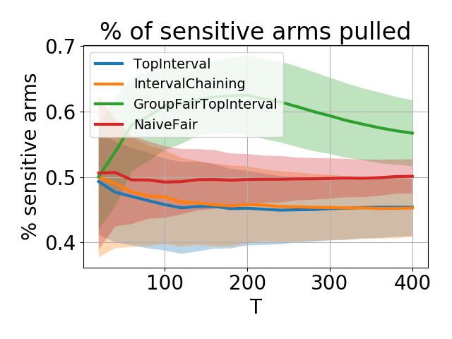
(a) Sensitive arm pulls (%)

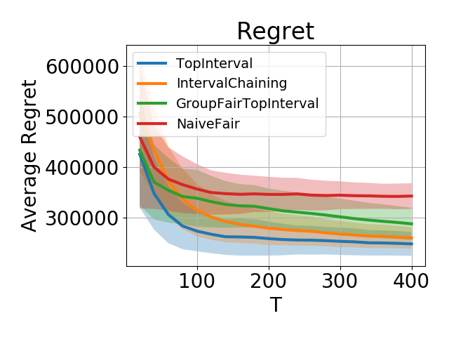
(b) Regret

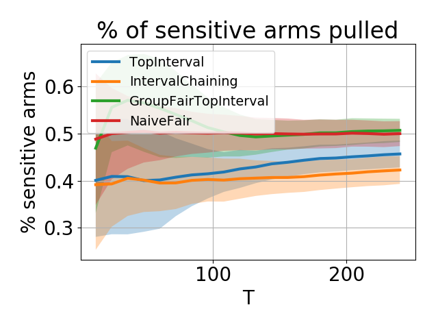
(c) Sensitive arm pulls (%)

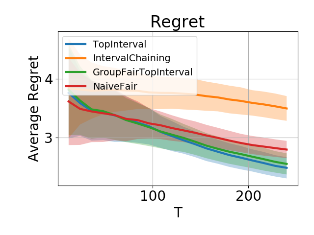
(d) Regret

Figure 3. Results of running contextual bandit algorithms on the family income and expenditure dataset (Figures 3(a) and 3(b)), as well as the COMPAS dataset (Figures 3(c) and 3(d)). Figures 3(a) and 3(c) show the percentage of pulls that were of sensitive arms. Figures 3(b) and 3(d) show the biased regret for each of the algorithms. Note that the “real” regret like that shown in the synthetic experiments cannot be calculated.

We run four different types of experiments: a) Varying the total budget for pulling arms ($T$) while setting number of arms $n=10$, error mean $\mu=10$, number of sensitive arms equal to 5, and context dimension $d=2$ (Figures 2(a) and 1(a)). b) Varying the total number of arms $n$ while setting total budget $T=1000$, error mean $\mu=10$, ratio of sensitive arms to 50%, and context dimension $d=2$ (Figures 2(b) and 1(b)). c) Varying the error mean $\mu$ while setting total budget $T=1000$, number of arms $n=10$, number of sensitive arms equal to 5, and context dimension $d=5$ (Figures 2(c) and 1(c)). d) Varying the number of sensitive arms while setting total budget $T=1000$, number of arms $n=10$, error mean $\mu=10$, and context dimension $d=2$ (Figures 2(d) and 1(d)).

The plots in Figure 1 show the percentage of times an algorithm pulled a sensitive arm over the full budget $T$. In order to be fair, the percentage of sensitive arms pulled should be proportional to the number of sensitive arms, i.e., when there are 5 sensitive arms out of 10 total, the percentage of sensitive arms pulled is roughly 50%. Figure 2 shows the perceived regret that includes bias $\psi$ as solid lines, and real regret that corrects bias (see Equations 2 and 3) as dashed lines. Algorithms with low real regret are considered ‘good’.

Figure 1(a) shows that once exploration is over, GroupFairTopInterval pulls sensitive arms roughly 50% of the time, matching the 50% of sensitive arms. Figure 2(a) shows that GroupFairTopInterval performs comparably on real regret as TopInterval performs on biased regret. This means GroupFairTopInterval should be used over TopInterval in contexts where bias is anticipated. NaiveFair performs poorly in the context of societal bias.

Figure 1(b) illustrates that IntervalChaining becomes more group fair as the number of arms increase. This is because many arms are chained together and therefore, arms are chosen uniformly at random. Figure 2(b) illustrates this random picking of arms as real regret and biased regret increases dramatically for IntervalChaining.

As expected, Figure 1(c) illustrates that when the error mean $\mu$ is large, both IntervalChaining and TopInterval choose fewer sensitive arms. This leads to a high real regret as shown in Figure 2(c). Following Kleinberg et al. (2016), Figure 2(c) also suggests that one cannot have both individual and group fairness in a scenario with high mean error. The randomness in NaiveFair leads to a very high regret for both perceived regret and real regret.

Figure 1(d) demonstrates the fairness property of proportionality. The percentage of sensitive arms pulled by GroupFairTopInterval matches the number of sensitive arms. As shown in Figure 2(d), the number of sensitive arms does not affect the real regret of GroupFairTopInterval.

5.3. Experiments on Real-World Data

After exploring GroupFairTopInterval on synthetic data, we move on to using both the Philippines family income and expenditure dataset on Kaggle and the ProPublica COMPAS dataset. When one looks at the gender and age breakdown in the family income dataset, one can see that quite often female heads of households make more money than males in the Philippines. This is most likely due to the large number of Filipino women who work out of the country; it is estimated that up to 20% of the GDP of the Philippines is actually remittances from these overseas—primarily female—workers. In fact, almost 60% of overseas workers are women and 75% of these women are between the ages of 25 and 44. In the COMPAS dataset ProPublica observed a societal bias over recidivism risk scores for African-Americans.

Experimental Setup.

Given the skew of high income coming from female head of households in the family income dataset, we treat the binary ‘Household Head Sex’ feature as the sensitive attribute. To create arms, we split up households based on ‘Household Head Age’ bucketed into the following five groups: (8, 27], (27, 45], (45, 63], (63, 81], and (81, 99]. We then have 10 different arms (for example, two arms would be Female head of household between 8 and 27, and Male head of household between 8 and 27).

Similarly, we treat African-American individuals from the COMPAS dataset as the sensitive attribute. We create arms by splitting up households based on the three age categories found in the data. We therefore have six different arms.

At each timestep $t$, we randomly select an individual from each arm. The context vector is the remaining features where any nominal features are transformed into integers. After an arm is pulled, a reward of the household income (for the family income dataset) or violent decile score (for COMPAS) is returned. We use these datasets for illustrative purposes.

Results.

We see the same behavior of arm pulls in the real world data. Figures 3(a) and 3(c) show that after a period of exploration, the percentage of sensitive arms (male-grouped arms) pulled gets very close to 50%, matching the proportion of sensitive-grouped arms.

Figures 3(b) and 3(d) are perhaps more interesting. Since we cannot measure the “real” regret without the bias we assumed from the sensitive-grouped arms, we consider the gap between GroupFairTopInterval and TopInterval as the price of fairness. The gap in regret is small compared to the increase in percentage of sensitive arms pulled. However, the gap in regret for NaiveFair is large in comparison. This suggests that explicitly learning a societal bias term will help in biased settings with low price to perceived regret. Note that there is a difference between regret scales for the two different datasets. This is due to the family income and expenditure dataset reporting regret in income, while the COMPAS dataset reports regret in recidivism score.

6. General Discussion & Ethical Implications of the Work

This work was directly motivated by research into bias found in machine learning models. There have also been calls to action for more research to be done on bias mitigation in online learning settings Chouldechova and Roth (2018); Bogen and Rieke (2018), specifically in multi-armed bandit settings Schumann et al. (2020) and related areas such as recommender systems Singh et al. (2020); Burke et al. (2020); Sonboli et al. (2020). Directly addressing these calls, in this work we propose a method of alleviating societal or measurement bias introduced into reward feedback. Using our CMAB model should help mitigate biased behaviors found in bandit systems currently in use Sweeney (2013b).

Additionally, as noted by O’Neil (2016), models can provide a biased feedback loop. We hope that by incorporating a societal bias term we can learn something about the bias that is being introduced. The coefficient vector will show which features are incorporating bias into the model. This allows users to address these features outside of the model and potentially find the sources of the societal bias. We do note that addressing societal bias and fixing the solution is a nontrivial task, the societal bias term provides the initial step of measurement.

On the other hand, as noted by Schumann et al. (2020), Shneiderman (2020b), and many others, humans should still be active participants in decision making. If models such as our CMAB model are used to replace more and more human decision makers, this could have unintended and potentially negative medium- and long-term side effects. All models should be monitored for biased feedback loops in the given contexts that they are being used O’Neil (2016).

Choosing a particular definition of fairness—conditioned on deciding that it is even appropriate to formally define a notion of fairness in the first place—is a morally-laden decision. We note that, as machine learning practitioners, in many societally-relevant applications it is paramount that we maintain an open dialogue with stakeholders. In this work, we analyze a sequential decision-making system under one particular definition, group fairness; it is certainly not the case that this is a one-size-fits-all solution that would be deployable without receiving input from that larger set of stakeholders. Indeed, recent research Saha et al. (2020) shows that non-expert users may have vastly varying degrees of comprehension of different definitions of fairness, and that the degree of comprehension may be a function in part of education level and other features that may correlate with measures of marginalization; this hints that the consequences of incorporating fairness definitions into machine-learning-based systems may not be uniformly understood by participants, and indeed that those participants who may be impacted the most by that change could comprehend that potential impact the least. In an allocative system like the one we describe in the main paper, nuanced considerations must be considered.

Our new definitions of reward (Equation 2) and regret (Equation 3) for the MAB setting provide an opportunity to look at biased data in a new light. In many cases, ground truths provided during learning are noisy with respect to sensitive groups. Additionally, debiased ground truths may be very expensive to receive or may take a long time to acquire. For instance, if looking at loans, true rewards of repayment may take years to receive. Or, for example, in hiring—the true reward of hiring an individual may take over a year to estimate, while the initial estimate may be influenced by a hiring team’s unconscious bias over features such as ethnicity, gender, or orientation.

Our proposed algorithm, GroupFairTopInterval, learns societal bias in the data while still being able to differentiate between individual arms. Previous solutions relied on setting ad-hoc thresholds, requiring some form of quota, or choosing groups uniformly at random. While it is true that GroupFairTopInterval can easily be extended to a case where we know that the average of a group is a constant offset from the other group. That being said, defining such offsets raises a host of other ethical questions. For instance, in the US, the EEOC (Equal Employment Opportunity Commision) poposed that the ratio of the most favored group compared to the least favored group must not be less than 0.8. Meanwhile, this type of comparison is forbidden in some countries Lieberman (2001). In any case, these prior solutions either lead to high regret, or require a large amount of domain knowledge for the chosen application.

7. Conclusion & Future Research

This paper explores group fairness in the contextual multi-armed bandit (MAB) setting. Our main contributions are: (1) we provide a new definition of reward and regret which captures societal bias; (2) we provide an algorithm that learns and corrects for that definition of societal bias; and (3) we empirically explore the effects different CMAB algorithms have in the setting of societal bias.

Future work could expand GroupFairTopInterval to enforce individual fairness within groups. Intersectional group fairness is also important to look at in the MAB setting where more than one type of sensitive attribute needs to be protected. Additionally, other group fairness definitions such as Equalized Opportunity should be converted to the MAB setting Hardt et al. (2016). Another interesting direction for future work is to mix ideas from the study of budget constrained bandits Ding et al. (2013); Wu et al. (2015) with our fairness definitions. We have also assumed individual arms have fixed group membership; generalizing to a setting where memberships in protected groups may change at every timestep $t$ would fit more real world applications.

Dickerson and Schumann were supported by NSF CAREER Award IIS-1846237, NSF Award CCF-1852352, NSF Award SMA-2039862, NIST MSE Award #20126334, DARPA GARD #HR00112020007, DARPA SI3-CMD #S4761, DoD WHS Award #HQ003420F0035, and ARPA-E DIFFERENTIATE Award #1257037. Mattei was supported by NSF Awards IIS-RI-2007955 and IIS-III-2107505. We thank Aviva Prins and Aravind Srinivasan for helpful comments on earlier versions of this paper, and the anonymous reviewers for helpful comments and constructive critiques.

Appendix A Additional Related Research

We now discuss, and appropriately compare and contrast, additional related research in settings similar to some aspects of our own model.

Fairness in ranking. A closely related area to our work is the research into fairness in rankings Singh and Joachims (2018), multi-stakeholder recommender systems Abdollahpouri and Burke (2019), and item allocation Benabbou et al. (2018, 2019). When algorithms return rankings for an individual to select from, one must pay attention to the ordering and the positioning of various groups Singh and Joachims (2018). One can see this as an application of the group fairness concept to the slates that are chosen for display. A particular aspect of recommendation systems that one needs to keep in mind is that often there are different stakeholders: the person receiving the recommendation, the company giving the recommendation, and the businesses that are the subjects of recommendation Abdollahpouri and Burke (2019). Finally, when goods are allocated, such as housing or subsidies one may need to observe both individual and group fairness Benabbou et al. (2018). Indeed, group fairness is specifically important in, e.g., Singapore, which has specifically enforced notions of group fairness when allocating public housing Benabbou et al. (2019).

Constrained reasoning in MAB. There is also significant recent work in constrained reasoning in the MAB setting. Balakrishnan et al. (2019) study the idea of learning constraints over pulling arms by observation in a pre-training phase. Wu et al. (2015) study constraints in both number of pulls per arm, as well as number of rounds where arms are available to be pulled. Wu et al. (2016) study a different flavor of constrained bandits where the learned policy cannot fall below a certain threshold; modeling the case where one wants to explore, but not suffer too much of a penalty over a status-quo policy. A related and perhaps interesting direction for future work is the work on bandits that are budget-constrained (without fairness considerations). Ding et al. (2013) study budget-constrained bandits where each arm also has an unknown cost distribution and one must learn a policy that maximizes reward and minimizes cost. Our formulation is not captured in the current literature on constrained and budgeted bandits and it is not obvious how to formalize a budget constraint as an inter-group fairness constraint. Indeed, a simplistic version of this would just lead to exhausting the budget of the “better” arm pulls before moving to the next best.

Legal motivation. Fairness in bandits is a particularly important area as the online, dynamic nature makes the task challenging and the use of bandits in a number of areas makes the problem particularly relevant. The motivating factor for group fairness is that one does not want to cause disparate impact, or the idea that groups should be treated differently based only on non-relevant aspects Feldman et al. (2015). Indeed, discrimination in certain areas including housing, credit, and jobs is forbidden in the US by the Civil Rights Act of 1965. It is specifically in these areas where bandit algorithms are deployed: advertising (where discrimination has been found) Sweeney (2013b), college admissions Schumann et al. (2019a), and interviewing Schumann et al. (2019b).

Appendix B Proofs

B.1. Two Groups

In order to prove Theorem 1, we first prove two lemmas.

Lemma 0.

The following holds for any $i$ at any time $t$, with probability at least $1-\delta$:

$$\left|\hat{\beta}_{i,t}\cdot x_{i,t}-(\beta_{i}\cdot x_{i,t}+\mathbbm{1}[i\in P_{1}]\psi_{P_{1}}\cdot x_{i,t})\right|\leq w_{i,t}.$$ (14)

Proof.

There are two cases: $i\in P_{1}$ or $i\not\in P_{1}$.

Focusing on the first case, inequality 14 becomes:

$$\left|\hat{\beta}_{i,t}\cdot x_{i,t}-\beta_{i}\cdot x_{i,t}\right|\leq w_{i,t}.$$

By the standard properties of OLS estimators Kuan (2004),

$$\hat{\beta}{i,t}\sim\mathcal{N}\left(\beta_{i},\sigma^{2}(X_{i,t}^{T},X_{i,t})^{-1}\right).$$

Then, for any fixed $x_{i,t}$:

$$\hat{\beta}_{i,t}\cdot x_{i,t}\sim\mathcal{N}\left(\beta_{i}\cdot x_{i,t},x_{i,t}^{T}\sigma^{2}(X_{i,t}^{T},X_{i,t})^{-1}x_{i,t}\right).$$

Using the definition of the Quantile function and the symmetric property of the normal distribution, with probability at least $1-\frac{\delta}{nT}$,

$$\hat{\beta}_{i,t}\sim\mathcal{N}\left(\beta_{i},\sigma^{2}(X_{i,t}^{T},X_{i,t})^{-1}\right).$$

Exploring the second case where $i\in P_{1}$, inequality 14 can be replaced with

$$\left|\hat{\beta}_{i,t}\cdot x_{i,t}-C_{i}\cdot x_{i,t}\right|\leq w_{i,t}$$

where $C_{i}=\beta_{i}+\psi_{P_{1}}$. Again, by the standard properties of OLS estimators $\hat{\beta}{i,t}\sim\mathcal{N}\left(C_{i},\sigma^{2}(X_{i,t}^{T},X_{i,t})^{-1}\right)$, we have for any fixed $x_{i,t}$:

$$\hat{\beta}_{i,t}\cdot x_{i,t}\sim\mathcal{N}\left(C_{i}\cdot x_{i,t},x_{i,t}^{T}\sigma^{2}(X_{i,t}^{T},X_{i,t})^{-1}x_{i,t}\right).$$

This uses the definition of the Quantile function and the symmetric property of the normal distribution, with probability at least $1-\frac{\delta}{nT}$.

Therefore, the probability that inequality 14 fails to hold for any $i$ at any timestep $t$ is at most $nT\cdot\frac{\delta}{nT}=\delta$. ∎

Lemma 0.

The following holds for any group $P_{j}$, any arm $i$, at any time $t$, with probability at least $1-\delta$:

$$\left|\hat{\psi}_{P_{j},t}\cdot x_{i,t}-\bar{\psi}_{P_{j}}\cdot x_{i,t}\right|\leq b_{P_{j},i,t}.$$ (15)

Proof.

By the standard properties of OLS estimators $\hat{\psi}_{P_{j},t}\sim\mathcal{N}\left(\bar{\psi}_{P_{j}},\sigma^{2}(\mathcal{X}_{P_{j},t}^{T},\mathcal{X}_{P_{j},t})^{-1}\right)$. For any fixed $x_{i,t}$,

$$\hat{\psi}_{i,t}\cdot x_{i,t}\sim\mathcal{N}\left(\bar{\psi}_{P_{j}}\cdot x_{i,t},x_{i,t}^{T}\sigma^{2}(\mathcal{X}_{P_{j},t}^{T},\mathcal{X}_{P_{j},t})^{-1}x_{i,t}\right).$$

Using the definition of the quantile function and the symmetric property of the normal distribution, with probability at least $1-\frac{\delta}{\frac{n}{|P_{j}|}T}$, inequality 15 holds. Therefore, the probability that this fails to hold for any $i$ at any timestep $t$ is at most $\frac{n}{|P_{j}|}T\cdot\frac{\delta}{\frac{n}{|P_{j}|}T}=\delta$. ∎

With Lemma 3 and Lemma 4, we can now prove Theorem 1.

Proof.

Regret for GroupFairTopInterval can be grouped into three terms for any $T_{1}\leq T$:

$$R^{*}(T) =\sum_{t:\ t\textit{ is an explore round}}\mathit{regret}(t)$$

$$+\sum_{t:\ t\textit{ is an exploit round and }t<T_{1}}\mathit{regret}(t)$$

$$+\sum_{t:\ t\textit{ is an exploit round and }t\geq T_{1}}\mathit{regret}(t)$$ (16)

Starting with the first term, define $p_{t}=\frac{1}{t^{1/3}}$ to be the probability that timestep $t$ is an exploration round. Then, for any $t$,

$$\sum_{t^{\prime}<t}p_{t^{\prime}}=\Theta(t^{2/3}).$$ (17)

We now focus on the third term of Equation 16, where $t$ is an exploit round and $t>T_{1}$. Throughout the rest of the proof we assume Lemma 3 and Lemma 4. Fix a exploit timestep $t$ where arm $i^{t}$ is played. Then,

$$\mathit{regret}(t) \leq 2w_{i^{t},t}+2b_{P_{1},i^{t},t}+2b_{P_{2},i^{t},t}$$

$$\leq 2\max_{i}\left(w_{i,t}+b_{P_{1},i,t}+b_{P_{2},i,t}\right)$$

$$\leq 2\left(\max_{i}w_{i,t}+\max_{i}b_{P_{1},i,t}+\max_{i}b_{P_{2},i,t}\right).$$ (18)

Note that:

$$w_{i,t}=Q_{\mathcal{N}\left(0,x_{i,t}\left(X_{i,t}^{T}X_{i,t}\right)^{-1}x_{i,t}^{T}\right)}\left(\frac{\delta}{2nT}\right).$$

Similarly,

$$b_{P_{j},i,t}=Q_{\mathcal{N}\left(0,x_{i,t}\left(\mathcal{X}_{P_{j},t}^{T}\mathcal{X}_{P_{j},t}\right)^{-1}x_{i,t}^{T}\right)}\left(\frac{\delta}{2\frac{n}{\left|P_{j}\right|}T}\right).$$

We first bound

$$x_{i,t}\left(X_{i,t}^{T}X_{i,t}\right)^{-1}x_{i,t} \leq||x_{i,t}||\lambda_{\max}\left(\left(X_{i,t}^{T}X_{i,t}\right)^{-1}\right)$$

$$=||x_{i,t}||\frac{1}{\lambda_{\min}\left(X_{i,t}^{T}X_{i,t}\right)}$$

$$\leq\frac{1}{\lambda_{\min}\left(X_{i,t}^{T}X_{i,t}\right)}$$ (19)

where the last inequality holds since $||x_{i,t}||\leq 1$ for all $i$ and $t$. Using similar logic,

$$x_{i,t}\left(\mathcal{X}_{P_{j},t}^{T}\mathcal{X}_{P_{j},t}\right)^{-1}x_{i,t}\leq\frac{1}{\lambda_{\min}\left(\mathcal{X}_{P_{j},t}^{T}\mathcal{X}_{P_{j},t}\right)}.$$ (20)

Let $G_{i,t}$ be the number of observations of arm $i$ with contexts drawn uniformly from the distribution for arm $i$ prior to timestep $t$. Similarly, let $\mathcal{G}_{P_{j},t}$ be the number of observations of group $P_{j}$ with contexts drawn uniformly from the distribution for group $P_{j}$ prior to timestep $t$. Let $L>\max_{t}\lambda_{\max}(x_{i,t}^{T},x_{i,t})$. For any $\alpha\in[0,1]$, using the superaddivity of minimum eigenvectors for positive semidefinite matrices, we get

$$\mathbb{E}\left[\lambda_{\min}(X_{i,t}^{T}X_{i,t})\right]\geq\frac{G_{i,t}}{d}\lambda_{\min_{i,d}}\geq\left\lfloor\frac{G_{i,t}}{d}\right\rfloor\lambda_{\min_{i,d}}.$$ (21)

Similarly,

$$\mathbb{E}\left[\lambda_{\min}(\mathcal{X}_{P_{j},t}^{T}\mathcal{X}_{P_{j},t})\right]\geq\frac{\mathcal{G}_{P_{j},t}}{d}\lambda_{\min_{P_{j},d}}\geq\left\lfloor\frac{\mathcal{G}_{P_{j},t}}{d}\right\rfloor\lambda_{\min_{P_{j},d}}.$$ (22)

Equation 21 implies that

$$\ \Pr_{X_{i,t}}\left[\lambda_{\min}(X_{i,t}^{T},X_{i,t})\leq\alpha\left\lfloor\frac{G_{i,t}}{d}\right\rfloor\lambda_{\min_{i,d}}\right]$$

$$\leq\Pr_{X_{i,t}}\left[\lambda_{\min}(X_{i,t}^{T},X_{i,t})\leq\alpha\mathbb{E}[\lambda_{\min}(X_{i,t}^{T}X_{i,t})]\right]$$ (23)

$$\leq\Pr_{X_{i,t}}\left[\lambda_{\min}(X_{i,t}^{T},X_{i,t})\leq\alpha\lambda_{\min}(\mathbb{E}[X_{i,t}^{T}X_{i,t}])\right]$$ (24)

$$\leq d\exp\left(\frac{-(1-\alpha)^{2}\lambda_{\min}(\mathbb{E}[X_{i,t}^{T}X_{i,t}])}{2L}\right)$$ (25)

$$\leq d\exp\left(\frac{-(1-\alpha)^{2}\mathbb{E}[\lambda_{\min}(X_{i,t}^{T}X_{i,t})]}{2L}\right)$$ (26)

$$\leq d\exp\left(\frac{-(1-\alpha)^{2}\left\lfloor\frac{G_{i,t}}{d}\right\rfloor\lambda_{\min_{i,d}}}{2L}\right)$$ (27)

where Inequalities 23 and 27 are from equation 21, Inequalities 24 and 26 are from Jensen’s inequality Mitzenmacher and Upfal (2017), and Inequality 25 uses a Matrix Chernoff Bound Mitzenmacher and Upfal (2017).

Using Inequality 27 after rearranging with probability $1-\delta$:

$$\lambda_{\min}(X_{i,t}^{T}X_{i,t})\geq\alpha\left\lfloor\frac{G_{i,t}}{d}\right\rfloor\lambda_{\min_{i,d}}$$ (28)

when

$$G_{i,t}\geq d\left(\frac{L}{(1-\alpha)^{2}\lambda_{\min_{i,d}}}\right)\left(\ln\frac{1}{\delta}+\ln d\right).$$ (29)

Using similar logic with probability $1-\delta$, we have

$$\lambda_{\min}(\mathcal{X}_{P_{j},t}^{T}\mathcal{X}_{P_{j},t})\geq\alpha\left\lfloor\frac{\mathcal{G}_{P_{j},t}}{d}\right\rfloor\lambda_{\min_{P_{j},d}}$$ (30)

when

$$\mathcal{G}_{P_{j},t}\geq d\left(\frac{L}{(1-\alpha)^{2}\lambda_{\min_{P_{j},d}}}\right)\left(\ln\frac{1}{\delta}+\ln d\right).$$ (31)

Using a multiplicative Chernoff bound Mitzenmacher and Upfal (2017) for a fixed timestep $t$ with probability $1-\delta^{\prime}$, the number of exploitation rounds prior to rounds $t$ will satisfy

$$\left|G_{t}-\sum_{t^{\prime}<t}p_{t^{\prime}}\right|\leq\sqrt{\ln\frac{2}{\delta^{\prime}}\sum_{t<t^{\prime}}p_{t^{\prime}}}$$ (32)

For a fixed $i$ and timestep $t$ using a multiplicative Chernoff bound, with probability $1-\delta^{\prime}$, the number of exploitation rounds for arm $i$ prior to round $t$ will satisfy

$$\left|G_{i,t}-\frac{G_{t}}{n}\right|\leq\sqrt{\ln\frac{2}{\delta^{\prime}}\frac{G_{t}}{n}}.$$ (33)

Similarly, for a fixed group $P_{j}$ and timestep $t$ with probaility $1-\delta^{\prime}$, the number of exploration rounds for group $P_{j}$ prior to round $t$ will satisfy

$$\left|\mathcal{G}_{i,t}-\frac{G_{t}}{|P_{j}|/n}\right|\leq\sqrt{\ln\frac{2}{\delta^{\prime}}\frac{G_{t}}{n/|P_{j}|}}$$ (34)

where $|P_{j}|$ is the size of group $P_{j}$.

Combining equations 32 and 33 with probability at least $1-2\delta^{\prime}$ for a fixed arm $i$ and timestep $t$, if $\sum_{t^{\prime}<t}P_{t^{\prime}}\geq 36n\ln^{2}\frac{2}{\delta^{\prime}}$ we have

$$\left|G_{i,t}-\frac{\sum_{t^{\prime}<t}p_{t^{\prime}}}{n}\right|\leq\frac{\sum_{t^{\prime}<t}p_{t^{\prime}}}{2n}.$$ (35)

Similarly, combining equations 32 and 34 with probability at least $1-2\delta^{\prime}$ for a fixed group $P_{j}$ and timestep $t$:

$$\left|\mathcal{G}_{i,t}-\frac{\sum_{t^{\prime}<t}P_{t^{\prime}}}{n/|P_{j}|}\right|\leq\frac{\sum_{t^{\prime}<t}p_{t^{\prime}}}{2n}.$$ (36)

Therefore, equation 28 holds with probability $1-\delta^{\prime}$ when

$$\frac{\sum_{t^{\prime}<t}p_{t}}{2n}\geq d\left(\frac{L}{(1-\alpha)^{2}\lambda_{\min_{i,d}}}\right)\left(\ln\frac{1}{\delta}+\ln d\right).$$ (37)

Similarly, equation 30 holds with probability $1-\delta^{\prime}$ when

$$\frac{\sum_{t^{\prime}<t}p_{t}}{2n/|P_{j}|}\geq d\left(\frac{L}{(1-\alpha)^{2}\lambda_{\min_{P_{j},d}}}\right)\left(\ln\frac{1}{\delta}+\ln d\right).$$ (38)

Therefore, since $n/|P_{j}|<n$, the number of rounds after which we have sufficient samples such that the estimators are well-concentrated is

$$T_{1}=\Theta\left(\min_{a}\left(\frac{dnL}{\lambda_{min_{a},d}}\left(\ln^{2}\frac{2}{\delta}+\ln d\right)\right)^{3/2}\right)$$ (39)

where $a\in[n]\cup P_{1}\cup P_{2}$.

Also note that for any $t\geq T_{1}$ we have

$$\sum_{t^{\prime}<t}p_{t^{\prime}}=\Omega\left(\min_{a}\left(\frac{dnL}{\lambda_{\min_{a,d}}}\left(\ln^{2}\frac{2}{\delta^{\prime}}+\ln d\right)\right)\right).$$ (40)

We can now bound the third term in Equation 16.

$$\sum_{t:\ t\textit{ is an exploit round and }t\geq T_{1}}regret(t)$$

$$\leq 2\sum_{t\geq T_{1}}\left(\max_{i}w_{i,t}+\max_{i}b_{P_{1},i,t}+\max_{i}b_{P_{2},i,t}\right)$$ (41)

$$\leq 2\sum_{t\geq T_{1}}\left(\max_{i}Q_{\mathcal{N}\left(0,\lambda_{\max}((X_{i,t}^{T}X_{i,t}))^{-1}\right)}\left(\frac{\delta}{2nT}\right)\right.$$

$$\ \ \ \ +\max_{i}Q_{\mathcal{N}\left(0,\lambda_{\max}((\mathcal{X}_{P_{1},t}^{T}\mathcal{X}_{P_{1},t}))^{-1}\right)}\left(\frac{\delta}{2\frac{n}{|P_{1}|}T}\right)$$

$$\ \ \ \ \left.+\max_{i}Q_{\mathcal{N}\left(0,\lambda_{\max}((\mathcal{X}_{P_{2},t}^{T}\mathcal{X}_{P_{2},t}))^{-1}\right)}\left(\frac{\delta}{2\frac{n}{|P_{2}|}T}\right)\right)$$

$$\leq 2\sum_{t\geq T_{1}}\left(Q_{\mathcal{N}\left(0,\frac{1}{\min_{i}\lambda_{\min}((X_{i,t}^{T}X_{i,t}))^{-1}}\right)}\left(\frac{\delta}{2nT}\right)\right.$$

$$\ \ \ \ +Q_{\mathcal{N}\left(0,\frac{1}{\min_{i}\lambda_{\min}((\mathcal{X}_{P_{1},t}^{T}\mathcal{X}_{P_{1},t}))^{-1}}\right)}\left(\frac{\delta}{2\frac{n}{|P_{1}|}T}\right)$$

$$\ \ \ \ \left.+\ Q_{\mathcal{N}\left(0,\frac{1}{\min_{i}\lambda_{\min}((\mathcal{X}_{P_{2},t}^{T}\mathcal{X}_{P_{2},t}))^{-1}}\right)}\left(\frac{\delta}{2\frac{n}{|P_{2}|}T}\right)\right)$$

$$\leq 2\sum_{t\geq T_{1}}\left(Q_{\mathcal{N}\left(0,\frac{1}{\min_{i}\alpha\left\lfloor\frac{G_{i,t}}{d}\right\rfloor\lambda_{\min_{i,d}}}\right)}\left(\frac{\delta}{2nT}\right)\right.$$

$$\ \ \ \ +Q_{\mathcal{N}\left(0,\frac{1}{\alpha\left\lfloor\frac{\mathcal{G}_{P_{1},t}}{d}\right\rfloor\lambda_{\min_{P_{1},d}}}\right)}\left(\frac{\delta}{2\frac{n}{|P_{1}|}T}\right)$$

$$\ \ \ \ \left.+\ Q_{\mathcal{N}\left(0,\frac{1}{\alpha\left\lfloor\frac{\mathcal{G}_{P_{2},t}}{d}\right\rfloor\lambda_{\min_{P_{2},d}}}\right)}\left(\frac{\delta}{2\frac{n}{|P_{2}|}T}\right)\right)+3\delta^{\prime}T$$ (42)

$$\leq 2\sum_{t\geq T_{1}}\left(\sqrt{\frac{\ln\frac{2nT}{\delta}}{\min_{i}\alpha\left\lfloor\frac{G_{i,t}}{d}\right\rfloor\lambda_{\min_{i,d}}}}\right.$$

$$\ \ \ \ +\sqrt{\frac{\ln\frac{2\frac{n}{|P_{1}|}T}{\delta}}{\min_{i}\alpha\left\lfloor\frac{\mathcal{G}_{P_{1},t}}{d}\right\rfloor\lambda_{\min_{P_{1},d}}}}$$

$$\ \ \ \ \left.+\sqrt{\frac{\ln\frac{2\frac{n}{|P_{2}|}T}{\delta}}{\min_{i}\alpha\left\lfloor\frac{\mathcal{G}_{P_{2},t}}{d}\right\rfloor\lambda_{\min_{P_{2},d}}}}\right)+6\delta^{\prime}T$$ (43)

$$\leq 2\sum_{t\geq T_{1}}\left(3\sqrt{\frac{\ln\frac{2nT}{\delta}}{\min_{i}\alpha\left\lfloor\frac{G_{i,t}}{d}\right\rfloor\lambda_{\min_{i,d}}}}\right)$$ (44)

$$=O\left(\sum_{t\geq T_{1}}\sqrt{d\frac{\ln\frac{2nT}{\delta}}{\min_{i}G_{i,t}\lambda_{\min_{i,d}}}}+\delta^{\prime}T\right)$$

$$=O\left(\sqrt{d\frac{\ln\frac{2nT}{\delta}}{\min_{i}\lambda_{\min_{i,d}}}}\sum_{t\geq T_{1}}\sqrt{\frac{1}{\min_{i}G_{i,t}}}+\delta^{\prime}T\right)$$

$$=O\left(\sqrt{d\frac{\ln\frac{2nT}{\delta}}{\min_{i}\lambda_{\min_{i,d}}}}\sum_{t\geq T_{1}}\sqrt{\frac{n}{\sum_{t^{\prime}<t}p_{t^{\prime}}}}+\delta^{\prime}T\right)$$

$$=O\left(\sqrt{d\frac{\ln\frac{2nT}{\delta}}{\min_{i}\lambda_{\min_{i,d}}}}\sum_{t\geq T_{1}}\sqrt{\frac{n}{t^{2/3}}}+\delta^{\prime}T\right)$$ (45)

$$=O\left(\sqrt{dn\frac{\ln\frac{2nT}{\delta}}{\min_{i}\lambda_{\min_{i,d}}}}\sum_{t\in[T_{1},T]}\frac{1}{t^{1/3}}+\delta^{\prime}T\right)$$

$$=O\left(\sqrt{dn\frac{\ln\frac{2nT}{\delta}}{\min_{i}\lambda_{\min_{i,d}}}}T^{2/3}+\delta^{\prime}T\right)$$ (46)

where (41) is due to Equation 18, (42) is due to Equations 21 and 22, (43) is due to Chernoff bounds, (44) is due to the fact that $\frac{n}{|P_{j}|}<n$ and $G_{P_{j},t}>\min_{i}G_{i,t}$, and (45) is due to Equation 17. Theorem 1 follows by combining Equations 16, 17, 39, and 46 and setting $\delta^{\prime}=\min\left(\frac{1}{3nT},\frac{1}{T^{1/3}}\right)$.

∎

B.2. Multiple Groups

Algorithm 3 GroupFairTopInterval (Multiple Groups)

0:  $\delta$, ($P_{1},\ldots,P_{m}$), $\rho$

1:  for $t=1\ldots T$ do

2:     with probability $\frac{1}{t^{1/3}}$, play $i_{t}\in_{R}\{1,\ldots,n\}$

3:     Else

4:        for $j=1\ldots,m$ do

5:           Let $\hat{\psi}_{P_{j},t}=\left(\mathcal{X}_{P_{j},t}^{T}\mathcal{X}_{P_{j},t}\right)^{-1}\mathcal{X}_{P_{j},t}^{T}\mathcal{Y}_{P_{j},t}$

6:        for $i=1\ldots n$ do

7:           Let $\hat{\beta}_{i,t}=\left(X_{i,t}^{T}X_{i,t}\right)^{-1}X_{i,t}^{T}Y_{i,t}^{T}$

8:           Let $F_{i,t}=\mathcal{N}\left(0,\sigma^{2}x_{i,t}\left(X_{i,t}^{T}X_{i,t}\right)^{-1}x_{i,t}^{T}\right)$

9:           Let $w_{i,t}=Q_{F_{i,t}}\left(\frac{\delta}{2nt}\right)$

10:           for $j$ where $i\in P_{j}$ do

11:              Let $\mathcal{F}_{P_{j},i,t}=\mathcal{N}\left(0,\sigma^{2}x_{i,t}\left(\mathcal{X}_{P_{j},t}^{T}\mathcal{X}_{P_{j},t}\right)x_{i,t}^{T}\right)$

12:              Let $b_{P_{j},i,t}=Q_{\mathcal{F}_{P_{j},i,t}}\left(\frac{\delta}{2\frac{n}{|P_{j}|}T}\right)$

13:              Let $\hat{u}_{i,t}=\hat{\beta}_{i,t}\cdot x_{i,t}+w_{i,t}+\rho-\hat{\psi}_{P_{j},t}\cdot x_{i,t}+b_{P_{j},i,t}$

14:        Play $\operatorname*{\arg\!\max}_{i}\hat{u}_{i,t}$ and observe reward $y_{i,t}$

In in order to prove Theorem 7, we first prove two lemmas.

Lemma 0.

The following holds for any $i$ at any time $t$, with probability at least $1-\delta$

$$\left|\hat{\beta}_{i,t}\cdot x_{i,t}-\left(\beta_{i}\cdot x_{i,t}+\sum_{j=1}^{m}\mathbbm{1}\left[i\in P_{j}\right]\psi_{P_{j}}\cdot x_{i,t}\right)\right|$$

$$\leq w_{i,t}$$ (47)

Proof.

Inequality 47 can be replaced with

$$\left|\hat{\beta}_{i,t}\cdot x_{i,t}-C_{i}\cdot x_{i,t}\right|\leq w_{i,t}$$

where $C_{i}=\beta_{i}+\psi_{P_{j}}$ and $i\in P_{j}$. By the standard properties of OLS estimators $\hat{\beta}_{i,t}\sim N\left(C_{i},\sigma^{2}(X_{i,t}^{T}X_{i,t})^{-1}\right)$. For any fixed $x_{i,t}$:

$$\hat{\beta}_{i,t}\cdot x_{i,t}\sim N\left(C_{i}\cdot x_{i,t},x_{i,t}^{T}\sigma^{2}(X_{i,t}^{T}X_{i,t})^{-1}x_{i,t}\right)$$

Using the definition of the quantile function and the symmetric property of the normal distribution, with probability at least $1-\frac{\delta}{nT}$, Inequality 47 holds. Therefore, the probability that inequality 47 fails to hold for any $i$ at any timestep $t$ is at most $nT\frac{\delta}{nT}=\delta$. ∎

Lemma 0.

The following holds for any group $P_{j}$, any arm $i$, at any timestep $t$, with probability at least $1-\delta$:

$$\left|\hat{\psi}_{P_{j},t}\cdot x_{i,t}-\psi_{P_{j},t}\cdot x_{i,t}\right|\leq b_{P_{j},i,t}.$$ (48)

Proof.

By the standard properties of OLS estimators,

$$\hat{\psi}_{P_{j},t}\sim N\left(\psi_{P_{j}},\sigma^{2}(\mathcal{X}_{P_{j},t}^{T}\mathcal{X}_{P_{j},t})^{-1}\right).$$

For any fixed $x_{i,t}$:

$$\hat{\psi}_{P_{j},t}\cdot x_{i,t}\sim N\left(\psi_{P_{j}}\cdot x_{i,t},x_{i,t}^{T}\sigma^{2}(\mathcal{X}_{P_{j},t}^{T}\mathcal{X}_{P_{j},t})^{-1}x_{i,t}\right).$$

Using the definition of the quantile function and the symmetric property of the normal distribution, with probability of at least $1-\frac{\delta}{\frac{n}{|P_{j}|}T}$ inequality 48 holds. Therefore the probability this fails to hold for any $i$ at timestep $t$ is at most $\frac{n}{|P_{j}|}T\frac{\delta}{\frac{n}{|P_{j}|}T}=\delta$. ∎

Theorem 7.

For $m$ groups $P_{1},\ldots,P_{m}$, where $\rho$ is the expected average reward, GroupFairTopInterval (Multiple Groups) has regret

$$R^{*}(T) =O\left(\sqrt{\frac{dn\ln\frac{2nT}{\delta}}{l}}T^{2/3}\right.$$

$$\left.+\left(\frac{dnmL}{l}\left(\ln^{2}\frac{2nT}{\delta}+\ln d\right)\right)^{2/3}\right)$$ (49)

where $l=\min_{i}\lambda_{min_{i,d}}$ and $L>\max_{t}\lambda_{\max}(x_{i,t}^{T}x_{i,t})$.

We can now prove Theorem 7.

Proof.

Assume that both Lemma 5 and Lemma 6 hold for all arms $i$ and all timesteps $t$.

Regret for GroupFairTopInterval (Multiple Groups) can be grouped into three terms for any $T_{1}\leq T$:

$$R^{*}(T) =\sum_{t:\ t\text{ is an explore round}}\mathit{regret}(t)$$

$$+\sum_{t:\ t\text{ is an exploit round and }t<T_{1}}\mathit{regret}(t)$$

$$+\sum_{t:\ t\text{ is an exploit round and }t\geq T_{1}}\mathit{regret}(t)$$ (50)

Starting with the first term in Equation 50, define $p_{t}=\frac{1}{t^{1/3}}$ to be the probability that timestep $t$ is an exploration round. Then, for any $t$,

$$\sum_{t^{\prime}<t}p_{t^{\prime}}=\Theta(t^{2/3})$$ (51)

Focusing on the third term of Equation 50, fix an exploit timestep $t$ where arm $i_{t}$ is played. Then,

$$\mathit{regret}(t) \leq 2w_{i_{t},t}+\max_{j}(2b_{P_{j},i_{t},t})$$

$$\leq 2\max_{i,j}(w_{i,t}+b_{P_{j},i,t})$$

$$\leq 2\left(\max_{i}w_{i,t}+\max_{i,j}b_{P_{j},i,t}\right)$$ (52)

From Algorithm 3, note that

$$w_{i,t}=Q_{N\left(0,x_{i,t}\left(X_{i,t}^{T}X_{i,t}\right)^{-1}x_{i,t}^{T}\right)}\left(\frac{\delta}{2nT}\right).$$

Similarly,

$$b_{P_{j},i,t}=Q_{N\left(0,x_{i,t}\left(\mathcal{X}_{P_{j},t}^{T}\mathcal{X}_{P_{j},t}\right)^{-1}x_{i,t}^{T}\right)}\left(\frac{\delta}{2\frac{n}{|P_{j}|}T}\right)$$

We will first bound $x_{i,t}\left(X_{i,t}^{T}X_{i,t}\right)^{-1}x_{i,t}^{T}$.

$$x_{i,t}\left(X_{i,t}^{T}X_{i,t}\right)^{-1}x_{i,t}^{T} \leq||x_{i,t}||\lambda_{\max}\left(\left(X_{i,t}^{T}X_{i,t}\right)^{-1}\right)$$

$$=||x_{i,t}||\frac{1}{\lambda_{\min}(X_{i,t}^{T}X_{i,t})}$$

$$\leq\frac{1}{\lambda_{\min}(X_{i,t}^{T}X_{i,t})}$$ (53)

where inequality 53 is due to $||x_{i,t}||\leq 1$ for all arms $i$ and all timesteps $t$.

Using similar logic:

$$x_{i,t}\left(\mathcal{X}_{P_{j},t}^{T}\mathcal{X}_{P_{j},t}\right)^{-1}x_{i,t}^{T}\leq\frac{1}{\lambda_{\min}\left(\mathcal{X}_{P_{j},t}^{T}\mathcal{X}_{P_{j},t}\right)}.$$ (54)

Let $G_{i,t}$ be the number of observations of arm $i$ with context $i$ drawn uniformly from the distribution for arm $i$ prior to timestep $t$. Similarly, let $\mathcal{G}_{P_{j},t}$ be the number of observations of group $P_{j}$ with context drawn uniformly from the distribution for group $P_{j}$ prior to timestep $t$. Let $L>\max_{t}\lambda_{\max}\left(x_{i,t}^{T}x_{i,t}\right)$.

For any $\alpha\in[0,1]$, using the superadditivity of minimum eugenvectors for positive semi-definite matrices, we get:

$$\mathbb{E}\left[\lambda_{\min}(X_{i,t}^{T}X_{i,t})\right] \geq\frac{G_{i,t}}{d}\lambda_{\min_{i,d}}$$

$$\geq\left\lfloor\frac{G_{i,t}}{d}\right\rfloor.$$ (55)

Similarly,

$$\mathbb{E}\left[\lambda_{min}(\mathcal{X}_{P_{j},t}^{T}\mathcal{X}_{P_{j},t})\right] \geq\left\lfloor\frac{G_{P_{j},t}}{d}\right\rfloor\lambda_{\min_{P_{j}.d}}.$$ (56)

Equation 55 implies that:

$$\Pr_{x_{i,t}}\left[\lambda_{\min}(X_{i,t}X_{i,t})\leq\alpha\left\lfloor\frac{G_{i,t}}{d}\right\rfloor\lambda_{\min_{i,d}}\right]$$

$$\leq\Pr_{x_{i,t}}\left[\lambda_{\min}(X_{i,t}^{T}X_{i,t})\leq\alpha\mathbb{E}\left[\lambda_{\min}(X_{i,t}^{T}X_{i,t})\right]\right]$$ (57)

$$\leq\Pr_{x_{i,t}}\left[\lambda_{\min}(X_{i,t}^{T}X_{i,t})\leq\alpha\lambda_{\min}\left(\mathbb{E}\left[X_{i,t}^{T}X_{i,t}\right]\right)\right]$$ (58)

$$\leq d\exp\left(\frac{-(1-\alpha)^{2}\lambda_{\min}\left(\mathbb{E}\left[X_{i,t}^{T}X_{i,t}\right]\right)}{2L}\right)$$ (59)

$$\leq d\exp\left(\frac{-(1-\alpha)^{2}\mathbb{E}\left[\lambda_{\min}\left(X_{i,t}^{T}X_{i,t}\right)\right]}{2L}\right)$$ (60)

$$\leq d\exp\left(\frac{-(1-\alpha)^{2}\left\lfloor\frac{G_{i,t}}{d}\right\rfloor\lambda_{\min_{i,d}}}{2L}\right)$$ (61)

where inequality 57 comes from inequality 55, inequality 58 is due to Jensen’s inequality, inequality 59 is due to a matrix Chernoff Bound, inequality 60 is due to Jensen’s inequality, and inequality 61 is due to inequality 55. After rearranging inequality 61, with probability $1-\delta$,

$$\lambda_{min}(X_{i,t}^{T}X_{i,t})\geq\alpha\left\lfloor\frac{G_{i,t}}{d}\right\rfloor\lambda_{\min_{i,d}}$$ (62)

when

$$G_{i,t}\geq d\left(\frac{L}{(1-\alpha)^{2}\lambda_{\min_{i,d}}}\right)\left(\ln{\frac{1}{\delta}}+\ln{d}\right).$$ (63)

Using similar logic with probability $1-\delta$, we have

$$\lambda_{\min}\left(\mathcal{X}_{P_{j},t}^{T}\mathcal{X}_{P_{j},t}\right)\geq\alpha\left\lfloor\frac{G_{P_{j},t}}{d}\right\rfloor\lambda_{\min_{P_{j},d}}$$ (64)

when

$$\mathcal{G}_{P_{j},t}\geq d\left(\frac{L}{(1-\alpha)^{2}\lambda_{\min_{P_{j},d}}}\right)\left(\ln\frac{1}{\delta}+\ln d\right).$$ (65)

Using a multiplicative Chernoff bound for a fixed timestep $t$ with probability $1-\delta^{\prime}$, the number of exploitation rounds prior to rount $t$ will satisfy

$$\left|G_{t}-\sum_{t^{\prime}<t}p_{t^{\prime}}\right|\leq\sqrt{\ln\frac{2}{\delta^{\prime}}\sum_{t^{\prime}<t}p_{t^{\prime}}}.$$ (66)

For a fixed $i$ and timestep $t$, using a multiplicative Chernoff bound for a fixed timestep $t$ with probability $1-\delta^{\prime}$, the number of exploitation rounds for arm $i$ prior to round $t$ will satisfy

$$\left|G_{i,t}-\frac{G_{t}}{n}\right|\leq\sqrt{\ln\frac{2}{\delta^{\prime}}\frac{G_{t}}{n}}$$ (67)

Similarly, for a fixed group $P_{j}$ and timestep $t$ with probability $1-\delta^{\prime}$, the number of exploration rounds for group $P_{j}$ prior to round $t$ will satisfy

$$\left|G_{P_{j},t}-\frac{G_{t}}{n/|P_{j}|}\right|\leq\sqrt{\ln\frac{2}{\delta^{\prime}}\frac{G_{t}}{n/|P_{j}|}}$$ (68)

where $|P_{j}|$ is the size of group $P_{j}$.

Combining inequality 66 and inequality 67, with probability $1-2\delta^{\prime}$ for a fixed arm $i$ and timestep $t$, if $\sum_{t^{\prime}<t}p_{t^{\prime}}\geq 36n\ln^{2}\frac{2}{\delta^{\prime}}$ we have

$$\left|G_{i,t}-\frac{\sum_{t^{\prime}<t}p_{t^{\prime}}}{n}\right|\leq\frac{\sum_{t^{\prime}<t}p_{t^{\prime}}}{2n}.$$ (69)

Similarly, combining inequality 66 and inequality 68 with probability at least $1-2\delta^{\prime}$ for a fixed group $P_{j}$ and fixed timestep $t$:

$$\left|G_{i,t}-\frac{\sum_{t^{\prime}<t}p_{t^{\prime}}}{n/|P_{j}|}\right|\leq\frac{\sum_{t^{\prime}<t}p_{t^{\prime}}}{2n/|P_{j}|}.$$ (70)

Therefore inequality 62 holds with probability $1-\delta^{\prime}$ when

$$\frac{\sum_{t^{\prime}<t}p_{t^{\prime}}}{2n}\geq d\left(\frac{L}{(1-\alpha)^{2}\lambda_{\min_{i,d}}}\right)\left(\ln\frac{1}{\delta}+\ln d\right).$$ (71)

Similarly, inequality 64 holds with probability $1-\delta^{\prime}$ when

$$\frac{\sum_{t^{\prime}<t}p_{t^{\prime}}}{2n/|P_{j}|}\geq d\left(\frac{L}{(1-\alpha)^{2}\lambda_{\min_{i,d}}}\right)\left(\ln\frac{1}{\delta}+\ln d\right).$$ (72)

Therefore, since $\frac{n}{|P_{j}|}<n$, the number of rounds after which we have sufficient samples such that the estimators are well-concentrated is

$$T_{1}=\Theta\left(\min_{a}\left(\frac{dnmL}{\lambda_{\min_{a,d}}}\left(\ln^{2}\frac{2}{\delta}+\ln d\right)\right)^{3/2}\right)$$ (73)

where $a\in[n]\cup P_{1}\cup\cdots\cup P_{m}$.

Also note that for any $t>T_{1}$ we have:

$$\sum_{t^{\prime}<t}p_{t^{\prime}}=\Omega\left(\min_{a}\left(\frac{dnmL}{2\min_{a,d}}\left(\ln^{2}\frac{2}{\delta^{\prime}}+\ln d\right)\right)\right).$$ (74)

Now we can bound the third term in equation 50.

$$\sum_{t:\ t\text{ is an exploit round and }t>T_{1}}\mathit{regret}(t)$$

$$\leq 2\sum_{t>T_{1}}\left(\max_{i}w_{i,t}+\max_{i,j}b_{P_{j},i,t}\right)$$ (75)

$$\leq 2\sum_{t>T_{1}}\left(\max_{i}Q_{N\left(0,\lambda_{\max}(X_{i,t}^{T}X_{i,t})^{-1}\right)}\left(\frac{\delta}{2nT}\right)\right.$$

$$\ \left.+\max_{j}Q_{N\left(0,\lambda_{\max}(\mathcal{X}_{P_{j},t}^{T}\mathcal{X}_{P_{j},t})^{-1}\right)}\left(\frac{\delta}{2\frac{n}{|P_{j}|}T}\right)\right)$$

$$\leq 2\sum_{t>T_{1}}\left(Q_{N\left(0,\frac{1}{\min_{i}\lambda_{\min}(X_{i,t}^{T}X_{i,t})}\right)}\left(\frac{\delta}{2nT}\right)\right.$$

$$\ \left.+\ Q_{N\left(0,\frac{1}{\min_{j}\lambda_{\min}(\mathcal{X}_{P_{j},t}^{T}\mathcal{X}_{P_{j},t})}\right)}\left(\frac{\delta}{2\frac{n}{|P_{j}|}T}\right)\right)$$

$$\leq 2\sum_{t>T_{1}}\left(Q_{N\left(0,\frac{1}{\min_{i}\alpha\left\lfloor\frac{G_{i,t}}{d}\right\rfloor\lambda_{\min_{i,d}}}\right)}\left(\frac{\delta}{2nT}\right)\right.$$

$$\ \left.+\ Q_{N\left(0,\frac{1}{\min_{j}\alpha\left\lfloor\frac{\mathcal{G}_{P_{j},t}}{d}\right\rfloor\lambda_{\min_{P_{j},d}}}\right)}\left(\frac{\delta}{2\frac{n}{|P_{j}|}T}\right)\right)+3\delta^{\prime}T$$ (76)

$$\leq 2\sum_{t>T_{1}}\left(\sqrt{\frac{\ln\frac{2nT}{\delta}}{\min_{i}\alpha\left\lfloor\frac{G_{i,t}}{d}\right\rfloor\lambda_{\min_{i,d}}}}\right.$$

$$\ \left.+\sqrt{\frac{\ln\frac{2\frac{n}{min_{j}|P_{j}|}T}{\delta}}{\min_{i}\alpha\left\lfloor\frac{\mathcal{G}_{P_{j},t}}{d}\right\rfloor\lambda_{\min_{i,d}}}}\right)+6\delta^{\prime}T$$ (77)

$$\leq 2\sum_{t>T_{1}}\left(2\sqrt{\frac{\ln\frac{2nT}{\delta}}{\min_{i}\alpha\left\lfloor\frac{G_{i,t}}{d}\right\rfloor\lambda_{\min_{i,d}}}}\right)+6\delta^{\prime}T$$ (78)

$$=O\left(\sum_{t>T_{1}}\sqrt{d\frac{\ln\frac{2nT}{\delta}}{\min_{i}G_{i,t}\lambda_{\min_{i,d}}}}+\delta^{\prime}T\right)$$

$$=O\left(\sqrt{d\frac{\ln\frac{2nT}{\delta}}{\min_{i}\lambda_{\min_{i,d}}}}\sum_{t>T_{1}}\sqrt{\frac{1}{\min_{i}G_{i,t}}}+\delta^{\prime}T\right)$$

$$=O\left(\sqrt{d\frac{\ln\frac{2nT}{\delta}}{\min_{i}\lambda_{\min_{i,d}}}}\sum_{t>T_{1}}\sqrt{\frac{n}{\sum_{t^{\prime}<t}p_{t^{\prime}}}}+\delta^{\prime}T\right)$$

$$=O\left(\sqrt{d\frac{\ln\frac{2nT}{\delta}}{\min_{i}\lambda_{\min_{i,d}}}}\sum_{t>T_{1}}\sqrt{\frac{n}{t^{2/3}}}+\delta^{\prime}T\right)$$ (79)

$$=O\left(\sqrt{dn\frac{\ln\frac{2nT}{\delta}}{\min_{i}\lambda_{\min_{i,d}}}}\sum_{t\in[T_{1},T]}\frac{1}{t^{1/3}}+\delta^{\prime}T\right)$$

$$=O\left(\sqrt{dn\frac{\ln\frac{2nT}{\delta}}{\min_{i}\lambda_{\min_{i,d}}}}T^{2/3}+\delta^{\prime}T\right)$$ (80)

where inequality 75 is due to equation 52, inequality 76 is due to equation 55 and equation 56, inequality 77 is due to a Chernoff bound, inequality 78 is due to the fact that $\frac{n}{\min_{j}|P_{j}|}<n$ and $\min_{j}\mathcal{G}_{P_{j},t}\geq min_{i}G_{i,t}$, and equation 79 is due to equation 51.

Combining equation 50, equation 51, equation 74, and equation 80 and setting $\delta^{\prime}=\min(\frac{1}{3nT},\frac{1}{T^{1/3}})$ we get Theorem 7. ∎

Appendix C Additional Experiments

Additionally to the experiments found in Section 5.2, we ran the following experiments and found no interesting effects:

1. Varying the range in which coefficients are chosen (between [0,c]) while setting the total budget $T=1000$, the number of arms $n=10$, the error mean $\mu=10$, the number of sensitive arms equal to 5, and the context dimension $d=2$ (Figures 4(a) and 5(a)).

2. Varying the context dimension while setting the total budget $T=1000$, the number of arms $n=10$, the error mean $\mu=10$, and the number of sensitive arms equal to 5 (Figures 4(b) and 5(b)).

3. Varying probability $\delta$ while setting the total budget $T=1000$, the number of arms $n=10$, the error mean $\mu=10$, the number of sensitive arms equal to 5, and the context dimension $d=2$ (Figures 4(c) and 5(c)).

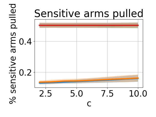
(a) $n=10$, $\mu=10$, number of sensitive arms = 5

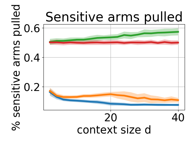
(b) $T=1000$, $\mu=10$, number of sensitive arms = 5

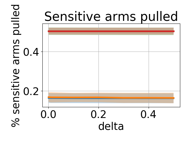
(c) $n=10$, $T=1000$, number of sensitive arms = 5

(d) legend

Figure 4. Percentage of total arm pulls that were pulled using sensitive arms.

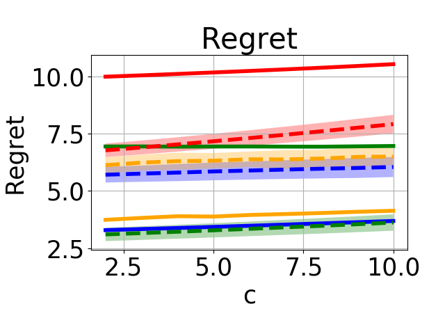
(a) $n=10$, $\mu=10$, number of sensitive arms = 5

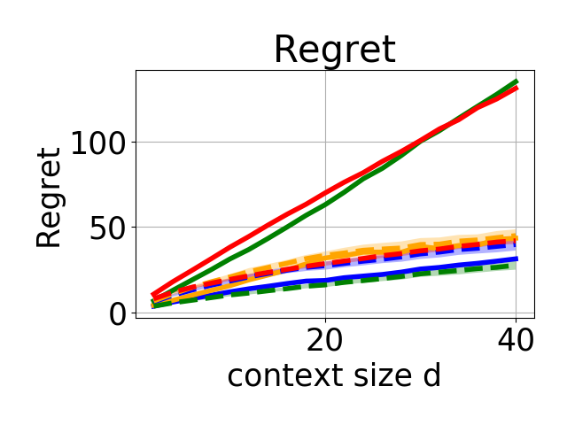
(b) $T=1000$, $\mu=10$, number of sensitive arms = 5

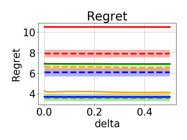
(c) $n=10$, $T=1000$, number of sensitive arms = 5

(d) legend

Figure 5. Regret for synthetic experiments. The solid lines are regret given the rewards received from pulling the arms (including the group bias). The dashed lines is the true regret (without the group bias).

References

- (1)
- Abdollahpouri and Burke (2019) Himan Abdollahpouri and Robin Burke. 2019. Multi-stakeholder Recommendation and its Connection to Multi-sided Fairness. arXiv preprint arXiv:1907.13158 (2019).
- Agrawal and Goyal (2013) Shipra Agrawal and Navin Goyal. 2013. Thompson Sampling for Contextual Bandits with Linear Payoffs. In Proceedings of the 30th International Conference on Machine Learning (ICML). 127–135.
- Auer et al. (2002) Peter Auer, Nicolò Cesa-Bianchi, and Paul Fischer. 2002. Finite-time Analysis of the Multiarmed Bandit Problem. Machine Learning 47, 2-3 (2002), 235–256.
- Balakrishnan et al. (2019) A. Balakrishnan, D. Bouneffouf, N. Mattei, and F. Rossi. 2019. Incorporating Behavioral Constraints in Online AI Systems. In Proc. of the 33rd AAAI Conference on Artificial Intelligence (AAAI).
- Belkin (2019) Douglas Belkin. 2019. SAT to give students ‘adversity score’ to capture social and economic background. The Wall Street Journal (2019).
- Bellamy et al. (2019) Rachel KE Bellamy, Kuntal Dey, Michael Hind, Samuel C Hoffman, Stephanie Houde, Kalapriya Kannan, Pranay Lohia, Jacquelyn Martino, Sameep Mehta, A Mojsilović, et al. 2019. AI Fairness 360: An extensible toolkit for detecting and mitigating algorithmic bias. IBM Journal of Research and Development (2019).
- Benabbou et al. (2019) Nawal Benabbou, Mithun Chakraborty, Edith Elkind, and Yair Zick. 2019. Fairness Towards Groups of Agents in the Allocation of Indivisible Items. In Proceedings of the 28th International Joint Conference on Artificial Intelligence (IJCAI). 95–101.
- Benabbou et al. (2018) Nawal Benabbou, Mithun Chakraborty, Xuan-Vinh Ho, Jakub Sliwinski, and Yair Zick. 2018. Diversity constraints in public housing allocation. In Proceedings of the 17th International Conference on Autonomous Agents and MultiAgent Systems (AAMAS). 973–981.
- Binns (2020) Reuben Binns. 2020. On the apparent conflict between individual and group fairness. In Proceedings of the 2020 Conference on Fairness, Accountability, and Transparency (FAT*). 514–524.
- Bogen (2019) Miranda Bogen. 2019. All the Ways Hiring Algorithms Can Introduce Bias. https://hbr.org/2019/05/all-the-ways-hiring-algorithms-can-introduce-bias [2019-08-22].
- Bogen and Rieke (2018) M. Bogen and A. Rieke. 2018. Help Wanted: An Examination of Hiring Algorithms, Equity, and Bias. Technical Report. Upturn.
- Burke et al. (2020) Robin Burke, Amy Voida, Nicholas Mattei, and Nasim Sonboli. 2020. Algorithmic Fairness, Institutional Logics, and Social Choice. In Harvard CRCS Workshop on AI for Social Good at 29th International Joint Conference on Artificial Intelligence (IJCAI 2020).
- Celis et al. (2019) L. Elisa Celis, Sayash Kapoor, Farnood Salehi, and Nisheeth Vishnoi. 2019. Controlling Polarization in Personalization: An Algorithmic Framework. In Proceedings of the Conference on Fairness, Accountability, and Transparency (FAT*). 160–169.
- Chen et al. (2020) Yifang Chen, Alex Cuellar, Haipeng Luo, Jignesh Modi, Heramb Nemlekar, and Stefanos Nikolaidis. 2020. Fair contextual multi-armed bandits: Theory and experiments. In Conference on Uncertainty in Artificial Intelligence (UAI). PMLR, 181–190.
- Chouldechova and Roth (2018) Alexandra Chouldechova and Aaron Roth. 2018. The Frontiers of Fairness in Machine Learning. CoRR abs/1810.08810 (2018). arXiv:1810.08810 http://arxiv.org/abs/1810.08810
- Claure et al. (2019) Houston Claure, Yifang Chen, Jignesh Modi, Malte Jung, and Stefanos Nikolaidis. 2019. Reinforcement Learning with Fairness Constraints for Resource Distribution in Human-Robot Teams. arXiv preprint arXiv:1907.00313 (2019).
- Corbett-Davies and Goel (2018) Sam Corbett-Davies and Sharad Goel. 2018. The measure and mismeasure of fairness: A critical review of fair machine learning. arXiv preprint arXiv:1808.00023 (2018).
- Ding et al. (2013) Wenkui Ding, Tao Qin, Xu-Dong Zhang, and Tie-Yan Liu. 2013. Multi-armed bandit with budget constraint and variable costs. In Twenty-Seventh AAAI Conference on Artificial Intelligence.
- Dwork et al. (2012) Cynthia Dwork, Moritz Hardt, Toniann Pitassi, Omer Reingold, and Richard Zemel. 2012. Fairness through awareness. In Proceedings of the 3rd Innovations in Theoretical Computer Science Conference. ACM, 214–226.
- Feldman et al. (2015) Michael Feldman, Sorelle A. Friedler, John Moeller, Carlos Scheidegger, and Suresh Venkatasubramanian. 2015. Certifying and Removing Disparate Impact. In Proceedings of the 21th ACM SIGKDD International Conference on Knowledge Discovery and Data Mining. 259–268.
- Hardt et al. (2016) Moritz Hardt, Eric Price, , and Nati Srebro. 2016. Equality of Opportunity in Supervised Learning. In Advances in Neural Information Processing Systems (NeurIPS). 3315–3323.
- Hossain et al. (2021) Safwan Hossain, Evi Micha, and Nisarg Shah. 2021. Fair Algorithms for Multi-Agent Multi-Armed Bandits. In Neural Information Processing Systems (NeurIPS).
- Joseph et al. (2016b) Matthew Joseph, Michael Kearns, Jamie Morgenstern, Seth Neel, and Aaron Roth. 2016b. Rawlsian fairness for machine learning. arXiv preprint arXiv:1610.09559 (2016).
- Joseph et al. (2016a) Matthew Joseph, Michael Kearns, Jamie H Morgenstern, and Aaron Roth. 2016a. Fairness in Learning: Classic and Contextual Bandits. In Advances in Neural Information Processing Systems (NeurIPS) 29, D. D. Lee, M. Sugiyama, U. V. Luxburg, I. Guyon, and R. Garnett (Eds.). 325–333.
- Kearns et al. (2018) Michael Kearns, Seth Neel, Aaron Roth, and Zhiwei Steven Wu. 2018. Preventing Fairness Gerrymandering: Auditing and Learning for Subgroup Fairness. In International Conference on Machine Learning. 2569–2577.
- Kleinberg et al. (2016) Jon Kleinberg, Sendhil Mullainathan, and Manish Raghavan. 2016. Inherent trade-offs in the fair determination of risk scores. Proceesings of the 2018 ACM International Conference on Measurement and Modeling of Computer Systems (2016).
- Kuan (2004) Chung-Ming Kuan. 2004. Classical least squares theory. http://homepage.ntu.edu.tw/~ckuan/pdf/et_ch3_Fall2009.pdf
- Lai and Robbins (1985) Tallai Andherbertrobbins Lai and Herbert Robbins. 1985. Asymptotically Efficient Adaptive Allocation Rules. Advances in Applied Mathematics 6, 1 (1985), 4–22.
- Li et al. (2010) Lihong Li, Wei Chu, John Langford, and Robert E Schapire. 2010. A contextual-bandit approach to personalized news article recommendation. In Proceedings of the 19th International Conference on World Wide Web (WWW). ACM, 661–670.
- Lieberman (2001) Robert Lieberman. 2001. A tale of two countries: the politics of color blindness in France and the United States. French Politics, Culture & Society 19, 3 (2001), 32–59.
- Littman et al. (2021) Michael L. Littman, Ifeoma Ajunwa, Guy Berger, Craig Boutilier, Morgan Currie, Finale Doshi-Velez, Gillian Hadfield, Michael C. Horowitz, Charles Isbell, Hiroaki Kitano, Karen Levy, Terah Lyons, Melanie Mitchell, Julie Shah, Steven Sloman, Shannon Vallor, and Toby Walsh. 2021. Gathering Strength, Gathering Storms: The One Hundred Year Study on Artificial Intelligence (AI100) 2021 Study Panel Report. Stanford University (2021).
- Liu et al. (2017) Yang Liu, Goran Radanovic, Christos Dimitrakakis, Debmalya Mandal, and David C Parkes. 2017. Calibrated fairness in bandits. In Workshop on Fairness, Accountability, and Transparency in Machine Learning (FAT-ML).
- Mary et al. (2015) Jérémie Mary, Romaric Gaudel, and Philippe Preux. 2015. Bandits and Recommender Systems. In Machine Learning, Optimization, and Big Data. 325–336.
- Misra et al. (2019) Kanishka Misra, Eric M Schwartz, and Jacob Abernethy. 2019. Dynamic Online Pricing with Incomplete Information Using Multiarmed Bandit Experiments. Marketing Science 38, 2 (2019), 226–252.
- Mitzenmacher and Upfal (2017) Michael Mitzenmacher and Eli Upfal. 2017. Probability and computing: randomization and probabilistic techniques in algorithms and data analysis. Cambridge university press.
- of the President et al. (2016) Executive Office of the President, Cecilia Munoz, Domestic Policy Council Director, Megan (US Chief Technology Officer Smith (Office of Science, Technology Policy)), DJ (Deputy Chief Technology Officer for Data Policy, Chief Data Scientist Patil (Office of Science, and Technology Policy)). 2016. Big data: A report on algorithmic systems, opportunity, and civil rights. Executive Office of the President.
- O’Neil (2016) Cathy O’Neil. 2016. Weapons of math destruction: How big data increases inequality and threatens democracy. Broadway Books.
- Patil et al. (2019) Vishakha Patil, Ganesh Ghalme, Vineet Nair, and Y Narahari. 2019. Achieving fairness in the stochastic multi-armed bandit problem. arXiv preprint arXiv:1907.10516 (2019).
- Rawls (1971) J. Rawls. 1971. A Theory of Justice. Harvard University Press.
- Ron et al. (2021) Tom Ron, Omer Ben-Porat, and Uri Shalit. 2021. Corporate Social Responsibility via Multi-Armed Bandits. In Proceedings of the 2021 ACM Conference on Fairness, Accountability, and Transparency (FAccT). 26–40.
- Rudin (2013) Cynthia Rudin. 2013. Predictive policing using machine learning to detect patterns of crime. Wired Magazine (2013).
- Saha et al. (2020) Debjani Saha, Candice Schumann, Duncan C. McElfresh, John P. Dickerson, Michelle L Mazurek, and Michael Carl Tschantz. 2020. Measuring Non-Expert Comprehension of Machine Learning Fairness Metrics. In Proceedings of the International Conference on Machine Learning (ICML).
- Schumann et al. (2019a) Candice Schumann, Samsara N. Counts, Jeffrey S. Foster, and John P. Dickerson. 2019a. The Diverse Cohort Selection Problem. In Proceedings of the 18th International Conference on Autonomous Agents and MultiAgent Systems (AAMAS). 601–609.
- Schumann et al. (2020) Candice Schumann, Jeffrey S Foster, Nicholas Mattei, and John P Dickerson. 2020. We Need Fairness and Explainability in Algorithmic Hiring. In Proceedings of the 19th International Conference on Autonomous Agents and MultiAgent Systems (AAMAS). 1716–1720.
- Schumann et al. (2019b) Candice Schumann, Zhi Lang, Jeffrey S. Foster, and John P. Dickerson. 2019b. Making the Cut: A Bandit-based Approach to Tiered Interviewing. In Proc. Advances in Neural Information Processing Systems (NeurIPS).
- Schumann et al. (2019c) Candice Schumann, Zhi Lang, Nicholas Mattei, and John P. Dickerson. 2019c. Group Fairness in Bandit Arm Selection. In NeurIPS Workshop on Machine Learning and Causal Inference for Improved Decision Making.
- Shneiderman (2020a) Ben Shneiderman. 2020a. Human-centered artificial intelligence: Reliable, safe & trustworthy. International Journal of Human–Computer Interaction 36, 6 (2020), 495–504.
- Shneiderman (2020b) Ben Shneiderman. 2020b. Human-centered Artificial Intelligence: Reliable, safe & trustworthy. International Journal of Human–Computer Interaction 36, 6 (2020), 495–504.
- Singh et al. (2020) Ashudeep Singh, Yoni Halpern, Nithum Thain, Konstantina Christakopoulou, Ed H. Chi, Jilin Chen, and Alex Beutel. 2020. Building Healthy Recommendation Sequences for Everyone: A Safe Reinforcement Learning Approach. In FAccTRec Workshop on Responsible Recommendation at RecSys-20.
- Singh and Joachims (2018) Ashudeep Singh and Thorsten Joachims. 2018. Fairness of exposure in rankings. In Proceedings of the 24th ACM SIGKDD International Conference on Knowledge Discovery & Data Mining. ACM, 2219–2228.
- Smith (1776) Adam Smith. 1776. The Wealth of Nations. New York: The Modern Library (1776).
- Sonboli et al. (2020) Nasim Sonboli, Robin Burke, Nicholas Mattei, Farzad Eskandanian, and Tian Gao. 2020. ”And the Winner Is…”: Dynamic Lotteries for Multi-group Fairness-Aware Recommendation. CoRR abs/2009.02590 (2020). arXiv:2009.02590
- Sutton and Barto (2017) Richard S. Sutton and Andrew Barto. 2017. Reinforcement Learning: An Introduction (2nd ed.). MIT Press.
- Sweeney (2013a) Latanya Sweeney. 2013a. Discrimination in online ad delivery. Commun. ACM 56, 5 (2013), 44–54.
- Sweeney (2013b) Latanya Sweeney. 2013b. Discrimination in online ad delivery. arXiv preprint arXiv:1301.6822 (2013).
- Tang et al. (2021) Yanhan Savannah Tang, Alan Andrew Scheller-Wolf, and Sridhar R Tayur. 2021. Generalized Bandits with Learning and Queueing in Split Liver Transplantation. Available at SSRN 3855206 (2021).
- Wang et al. (2021) Lequn Wang, Yiwei Bai, Wen Sun, and Thorsten Joachims. 2021. Fairness of Exposure in Stochastic Bandits. In International Conference on Machine Learning (ICML).
- Wexler et al. (2019) James Wexler, Mahima Pushkarna, Tolga Bolukbasi, Martin Wattenberg, Fernanda Viégas, and Jimbo Wilson. 2019. The What-If Tool: Interactive probing of machine learning models. IEEE transactions on visualization and computer graphics (2019).
- Wu et al. (2015) Huasen Wu, Rayadurgam Srikant, Xin Liu, and Chong Jiang. 2015. Algorithms with logarithmic or sublinear regret for constrained contextual bandits. In Advances in Neural Information Processing Systems. 433–441.
- Wu et al. (2016) Yifan Wu, Roshan Shariff, Tor Lattimore, and Csaba Szepesvári. 2016. Conservative bandits. In International Conference on Machine Learning. 1254–1262.
- Young (1995) H Peyton Young. 1995. Equity: in theory and practice. Princeton University Press.