IPMU19-0176

Kazushi Ueda^a and Yutaka Yoshida^b

^aGraduate School of Mathematical Sciences, The University of Tokyo,

3-8-1 Komaba Meguro-ku, Tokyo 153-8914 Japan

kazushi@ms.u-tokyo.ac.jp

^bKavli IPMU (WPI), UTIAS, The University of Tokyo
Kashiwa, Chiba 277-8583, Japan
yutaka.yoshida@ipmu.jp

3d $\mathcal{N}=2$ Chern–Simons–matter theory, Bethe ansatz, and quantum $K$-theory of Grassmannians

1 Introduction and summary

$\mathcal{N}=(2,2)$ supersymmetric gauged linear sigma models (GLSM) in two dimensions [1] play important roles in connection with quantum cohomology, Gromov–Witten invariants, and mirror symmetry. Correlation functions of the vector multiplet scalars of abelian A-twisted GLSM on the two-sphere $S^{2}$ was studied in [2]. When the Higgs branch of $\mathcal{N}=(2,2)$ GLSM is a toric Fano manifold, the three-point correlation functions give the three-point genus-zero Gromov–Witten invariants of that manifold. When the Higgs branch is a Calabi–Yau 3-fold, the identification of the three-point functions with the B-model Yukawa couplings of the mirror is known as toric residue mirror symmetry [3, 4, 5, 6, 7]. Three-point functions of non-abelian A-twisted GLSMs on $S^{2}$, possibly with the $\Omega$-background, are computed in [8] using supersymmetric localization. It was suggested in [9] that the resulting formulas give genus-zero quasimap invariants of the space of Higgs branch vacua of the GLSM, and proved mathematically in [10] for Grassmannians and their Calabi–Yau complete intersections defined by equivariant vector bundles. It follows that the twisted chiral ring of 2d A-twisted GLSM, whose Higgs branch is the Grassmannian, agrees with the small quantum cohomology ring of the Grassmannian.

When a supersymmetric quantum field theory on a manifold $M$ is related to a cohomological object, an $S^{1}$ uplift of the theory, i.e., a supersymmetric quantum field theory on $S^{1}\times M$, is often related to a $K$-theoretic object. A typical example is Nekrasov’s instanton partition functions; roughly speaking, instanton partition functions on $\mathbb{R}^{4}$ [11] are integrals of cohomology classes over instanton moduli spaces [12], whereas five-dimensional instanton partition functions on $S^{1}\times\mathbb{R}^{4}$ [13] are indices of instanton moduli spaces ($K$-theoretic instanton partition functions) [14]. Hence it is natural to expect the existence of 3d (topologically twisted) supersymmetric gauge theories relevant to quantum $K$-theory [15], which is a $K$-theoretic analogue of quantum cohomology.

In this paper, we establish a relation between certain 3d topologically twisted supersymmetric gauge theories and the quantum $K$-rings of Grassmannians. Although there are earlier works in this direction, starting with [16] which pointed out a similarity between the small $K$-theoretic $J$-function of $\mathbb{P}^{M-1}$ and the vortex partition function of a certain 3d $U(1)$ gauge theory in the context of open BPS state counting, to our best knowledge, an identification of the small quantum $K$-ring of Grassmannians (or even projective spaces) with the level of precision of this paper is new.

To find the precise relation between the 3d supersymmetric theories and the quantum $K$-ring of Grassmannians, we focus on Bethe/Gauge correspondence. It was pointed out in [17, 18] that the saddle point equations of the mass deformations of a 2d $\mathcal{N}=(4,4)$ $U(N)$ GLSM coincide with the Bethe ansatz equation of the spin-$\frac{1}{2}$ XXX spin chain. The relation between the twisted chiral ring and the quantum cohomology mentioned above implies that the Bethe ansatz equation is closely related to the relations of the equivariant quantum cohomology ring of the cotangent bundle of the Grassmannian, which appears as the Higgs branch of the $\mathcal{N}=(4,4)$ GLSM. See e.g. [19] for a mathematical formulation of this observation.

For the quantum cohomology of the Grassmannian, a description in terms of the algebraic Bethe ansatz of a five-vertex model is given by Gorbounov–Korff [20]. In a subsequent work [21], they introduced a finite-dimensional commutative Frobenius algebra depending on a parameter $\beta$. They showed that the Frobenius algebra with $\beta=-1$ is isomorphic to the small quantum $K$-ring of Grassmannian and the Frobenius algebra with $\beta=0$ reproduces their previous result on the quantum cohomology in [20].

By using supersymmetric localization formulas, we show that the saddle point equations of the 3d $U(N)$ Chern–Simons-matter theory with $M$ chiral multiplets coincide with the Bethe ansatz equations for $\beta=-1$. This implies that the operator product expansions (OPEs) of Wilson loop operators $\mathcal{W}_{\lambda}$ can be identified with the quantum products of the equivariant quantum $K$-theory ring $QK_{T}(\mathrm{Gr}(N,M))$ of the Grassmannian;

$$\mathcal{W}_{\mu}\mathcal{W}_{\nu}=\sum_{\lambda}C_{\mu\nu}^{\lambda}\mathcal{W}_{\lambda}\Longleftrightarrow[\mathcal{O}_{\mu}]\star[\mathcal{O}_{\nu}]=\sum_{\lambda}C_{\mu\nu}^{\lambda}[\mathcal{O}_{\lambda}].$$ (1.1)

Here $\star$ is the quantum product in $QK_{T}(\mathrm{Gr}(N,M))$ and $[\mathcal{O}_{\lambda}]$’s are the $K$-theory classes of Schubert varieties of the Grassmannian. We also revisit the relation between A-twisted 2d GLSM and quantum cohomology from the viewpoint of Bethe/Gauge correspondence, and derive an isomorphism of the twisted chiral ring with the equivariant small quantum cohomology of the Grassmannians.

Generalizations of the supersymmetric localization formula from $S^{1}\times S^{2}$ (resp. $S^{2}$) to higher genus cases $S^{1}\times\Sigma_{g}$ (resp. $\Sigma_{g}$) were studied in [23, 24]. We show that the correlation functions at higher genus can be identified with the correlation functions of the 2d topological quantum field theories (TQFTs) associated with the Frobenius algebra.

Besides the correspondence between the algebra of Wilson loops in the topologically twisted CS–matter theories and the quantum $K$-rings of Grassmannians, we discuss several other aspects of CS–matter theories; CS–matter theories with $\Omega$-background, $K$-theoretic $I$-functions of Grassmannians with level structures, supersymmetric index on $S^{1}\times D^{2}$, and deformations of Verlinde algebra in terms of indices over moduli stacks of $G$-bundles on Riemann surfaces.

This article is organized as follows. In section 2.1, we recall results by Gorbounov–Korff which will be used later to show the relation between quantum $K$-ring (resp. quantum cohomology) and CS–matter theory (resp. GLSM). In section 2.2, we compute the correlation functions of 2d TQFT on a genus $g$ surface associated with the Frobenius algebra. In section 2.3, we evaluate the inner product of the on-shell Bethe vectors by the Izergin–Korepin method. In section 3, we show that the genus $g$ correlation function of the 2d TQFT associated with the Frobenius algebra with $\beta=0$ agrees with the genus $g$ correlation functions of the A-twisted GLSM. In section 4, which is the main part of our paper, we study the correspondence between CS–matter theories and the quantum $K$-theory of Grassmannians. In section 4.1, we show that the supersymmetric localization formulas of the correlation functions of Wilson loops on $S^{1}\times\Sigma_{g}$ agree with the genus $g$ correlation functions of 2d TQFT associated with the Frobenius algebra with $\beta=-1$. These equalities lead to the isomorphism between the algebras of Wilson loops and the quantum $K$-ring of Grassmannians. In section 4.2, we turn on the $\Omega$-background and show that the partition function of topologically twisted CS–matter theory with specific choices of CS levels factorizes to a pair of $K$-theoretic $I$-functions, and discuss the relation between CS levels and level structures of quantum $K$-theory. In section 4.3, we show that $K$-theoretic $I$-function derived in section 4.2 can be derived from a supersymmetric index on $S^{1}\times D^{2}$. In section 5, we discuss connections between CS–matter theories and deformations of Verlinde algebra.

Note added: When our paper was being completed, we became aware of the paper [25] by H. Jockers et al. on the arXiv, which has partial overlap with some results in our paper.

2 Quantum $K$-ring, quantum cohomology and algebraic Bethe ansatz

Gorbounov–Korff [21] defined a Frobenius algebra depending on a parameter $\beta$ in terms of algebraic Bethe ansatz. The elements of the Frobenius algebra are defined by the $N$ excitations (particle states) in the Hilbert space of the quantum integrable system with $M$-sites. The Frobenius bilinear form is defined in terms of the inner product of states and dual of states in the Hilbert spaces. They showed that the structure constants in the spin basis agree with the structure constants of the equivariant quantum $K$-ring of Grassmannian ${QK}_{T}(\mathrm{Gr}(N,M))$ for $\beta=-1$ and the equivariant quantum cohomology of Grassmannian ${QH}_{T}(\mathrm{Gr}(N,M))$ for $\beta=0$.

In section 2.1, we summarize results from [21] which will be useful later. In particular, we recall the definition and properties of the Frobenius algebra introduced in [21]. In section 2.2, we describe the correlation functions of the 2d TQFT associated with the Frobenius algebra. In section 2.3, we evaluate the on-shell square norm of Bethe vectors and dual Bethe vectors.

2.1 Results of Gorbounov–Korff

First we introduce the R-matrix and L-operator which characterize the quantum integrable model in [21]. The R-matrix ${\sf R}({x},{y})\in\mathrm{End}[\mathbb{C}^{2}({x})\otimes\mathbb{C}^{2}({y})]$ is defined by

$${\sf R}({x},{y}):=\left(\begin{array}[]{cccc}1&0&0&0\\ 0&0&1&0\\ 0&1+\beta({y}\ominus{x})&{y}\ominus{x}&0\\ 0&0&0&1\\ \end{array}\right),$$ (2.5)

where $\ominus$ is defined in Appendix A. The R-matrix satisfies the following Yang-Baxter equation:

$${\sf R}_{12}({x,y}){\sf R}_{13}({x,z}){\sf R}_{23}({y,z})={\sf R}_{13}({x,z}){\sf R}_{23}({y,z}){\sf R}_{12}({x,y}),$$ (2.6)

with

$${\sf R}_{12}({x,y}):={\sf R}({x,y})\otimes\mathbb{I}_{2},$$ (2.7)

$${\sf R}_{23}({x,y}):=\mathbb{I}_{2}\otimes{\sf R}({x,y}),$$ (2.8)

$${\sf R}_{13}({x,y}):=(\mathbb{I}_{2}\otimes{\sf P}){\sf R}_{12}({x,y})(\mathbb{I}_{2}\otimes{\sf P}).$$ (2.9)

Here $\mathbb{I}_{2}$ is the identity matrix of size two and ${\sf P}$ is a permutation matrix defined by ${\sf P}(v\otimes u)=u\otimes v$ for $u,v\in\mathbb{C}^{2}$. The L-operator ${\sf L}({x|t})\in\mathrm{End}[\mathbb{C}^{2}({x})\otimes\mathbb{C}^{2}({t})]$ is defined by

$${\sf L}({x|t})=\left(\begin{array}[]{cc}\sigma^{+}\sigma^{-}+({x}\ominus{t})\sigma^{-}\sigma^{+}&(1+\beta({x}\ominus{t}))\sigma^{+}\\ \sigma^{-}&\sigma^{-}\sigma^{+}\\ \end{array}\right),$$ (2.12)

with

$$\sigma^{+}=\left(\begin{array}[]{cc}0&0\\ 1&0\\ \end{array}\right),\quad\sigma^{-}=\left(\begin{array}[]{cc}0&1\\ 0&0\\ \end{array}\right).$$ (2.17)

The R-matrix and the L-operator satisfy the following Yang-Baxter type relation (RLL relation);

$${\sf R}_{12}({x,y})\left({\sf L}({x|t})\otimes{\sf L}({y|t})\right)=\left({\sf L}({y|t})\otimes{\sf L}({x|t})\right){\sf R}_{12}({x,y}).$$ (2.18)

From (2.18) one can show that the monodromy matrix ${\sf M}({x|t})\in\mathrm{End}[\mathbb{C}^{2}({x})\otimes\otimes_{i=1}^{M}\mathbb{C}^{2}({t}_{i})]$ defined by

$${\sf M}({x|t})=\left(\begin{array}[]{cc}{\sf A}({x|t})&{\sf B}({x|t})\\ {\sf C}({x|t})&{\sf D}({x|t})\\ \end{array}\right):={\sf L}({x}|{t}_{M})\cdots{\sf L}({x}|{t}_{2}){\sf L}({x}|{t}_{1})$$ (2.21)

also satisfies the Yang-Baxter type relation (RTT relation)

$${\sf R}_{12}(x,y)\left({\sf M}(x|t)\otimes{\sf M}(y|t)\right)=\left({\sf M}(y|t)\otimes{\sf M}(x|t)\right){\sf R}_{12}(x,y).$$ (2.22)

Here ${\sf L}({x}|{t}_{i})$ non-trivially acts on $\mathbb{C}^{2}({x})\otimes\mathbb{C}^{2}({t}_{i})$. (2.22) gives the sixteen relations between four $2^{M}\times 2^{M}$ matrices ${\sf A}(x|t),{\sf B}(x|t),{\sf C}(x|t)$ and ${\sf D}(x|t)$ listed in appendix B. The twisted transfer matrix is defined by the trace taken over the auxiliary space as

$${\sf T}(y|t):=\mathrm{Tr}\left({\sf M}(y|t)\left(\begin{array}[]{cc}1&0\\ 0&q\\ \end{array}\right)\right)={\sf A}({y|t})+q{\sf D}({y|t}).$$ (2.25)

The periodic boundary condition is given by $q=1$. Note that the twist parameter $q$ will be identified with the quantum parameter of the quantum $K$-ring for $\beta=-1$ and the quantum parameter of the quantum cohomology for $\beta=0$. From the relation (2.22), the transfer matrices commute with each other:

$$[{\sf T}({y}|t),{\sf T}({y^{\prime}|t})]=0.$$ (2.26)

The coefficients of ${y}^{l}$ for $l=0,1,\cdots$ in ${\sf T}({y}|{t})$ give conserved charges.

The states and dual states on which ${\sf A,B,C,D}$ act are defined as follows. First we introduce a basis of the $2^{M}$-dimensional space $\otimes_{i=1}^{M}\mathbb{C}^{2}({t}_{i})$ by

$$\otimes_{i=1}^{M}{v}_{\ell_{i}}\,\text{ with }\,\ell_{i}\in\{0,1\},$$ (2.27)

where $v_{0}$ and $v_{1}$ are defined by

$$v_{0}:=\left(\begin{array}[]{c}1\\ 0\\ \end{array}\right),v_{1}:=\left(\begin{array}[]{c}0\\ 1\\ \end{array}\right),$$ (2.32)

and we also introduce the dual space spanned by

$$\otimes_{i=1}^{M}{v}_{\ell_{i}}^{T}\,\text{ with }\,\ell_{i}\in\{0,1\}.$$ (2.33)

The $2^{M}$-dimensional space is decomposed to the direct sum $\bigoplus_{N=0}^{M}\mathcal{V}_{N,M}$, where $\mathcal{V}_{N,M}$ is a $M!/N!(M-N)!$-dimensional vector space spanned by the vectors $\otimes_{i=1}^{M}{v}_{\ell_{i}}$ with $\sum_{i=1}^{M}\ell_{i}=N$. The vectors $\otimes_{i=1}^{M}{v}_{\ell_{i}}$ with $\sum_{i=1}^{M}\ell_{i}=N$ are in one-to-one correspondence with the elements of a set of partitions $\mathcal{P}_{N,M}$ defined by

$$\mathcal{P}_{N,M}:=\{\lambda=(\lambda_{1},\dots\lambda_{N})|M-N\geq\lambda_{1}\geq\lambda_{2}\geq\cdots\geq\lambda_{N}\geq 0\}.$$ (2.34)

We define a vector $|v_{\lambda}\rangle$ by $\otimes_{i=1}^{M}{v}_{\ell_{i}}$ which correspond to a partition $\lambda\in\mathcal{P}_{N,M}$ . We call $\{|v_{\lambda}\rangle\}_{\lambda\in\mathcal{P}_{N,M}}$ as the spin basis of $\mathcal{V}_{N,M}$. The dual spin basis $\{\langle v_{\lambda}|\}_{\lambda\in\mathcal{P}_{N,M}}$ for the dual space of $\mathcal{V}_{N,M}$ is defined in a similar way and the inner products satisfy $\langle v_{\lambda}|v_{\mu}\rangle=\delta_{\lambda\mu}$. We define $\emptyset$ by $\emptyset:=(0,\cdots,0)\in\mathcal{P}_{N,M}.$

The pseudo vacuum $|0\rangle$ and the dual pseudo vacuum $\langle 0|$ are defined by

$$|0\rangle:=\otimes_{i=1}^{M}v_{1},\quad\langle 0|:=\otimes_{i=1}^{M}v_{1}^{T}.$$ (2.35)

The ${\sf A},{\sf B},{\sf C},{\sf D}$ act on the pseudo vacuum as

$${\sf A}({y}|{t})|0\rangle={\sf a}({y},{t})|0\rangle,\,\langle 0|{\sf B}({y}|{t})=0,\,{\sf C}({y}|{t})|0\rangle=0,\,{\sf D}({y}|{t})|0\rangle={\sf d}({y},{t})|0\rangle,$$ (2.36)

with

$${\sf a}({y},{t}):=\prod_{i=1}^{M}(y\ominus t_{i}),\quad{\sf d}({y},{t}):=1.$$ (2.37)

Suppose $\prod_{a=1}^{N}{\sf B}({y}_{a})|0\rangle$ is an eigen vector of the transfer matrix (2.25), then $\{{y}_{1},\cdots,{y}_{N}\}$ have to satisfy the following system of equations called the Bethe ansatz equation:

$$\frac{(-1)^{N-1}q(1+\beta y_{a})^{N}}{\prod_{b=1}^{N}(1+\beta y_{b})\prod_{i=1}^{M}(y_{a}\ominus t_{i})}=1,\quad a=1,\cdots,N.$$ (2.38)

A root $\{y_{a}\}_{a=1}^{N}$ of the Bethe ansatz equation is called as a Bethe root. When $\{y_{a}\}_{a=1}^{N}$ is a Bethe root, $\prod_{a=1}^{N}{\sf B}(y_{a})|0\rangle$ $(\text{resp. }\langle 0|\prod_{a=1}^{N}{\sf C}(y_{a})$) is called an on-shell Bethe vector, (resp. on-shell dual Bethe vector), vice versa. When $\{y_{a}\}_{a=1}^{N}$ is indeterminate, Bethe vectors are called off-shell.

The Bethe ansatz equation has $\frac{M!}{N!(M-N)!}$ distinct Bethe roots. The $\frac{M!}{N!(M-N)!}$ Bethe roots are characterized by the partitions in $\mathcal{P}_{N,M}$ as

$${y}_{\lambda}=(y_{\lambda_{N}+1},\cdots,y_{\lambda_{2}+N-1},y_{\lambda_{1}+N})\,\text{ for }\lambda\in\mathcal{P}_{M,N},$$ (2.39)

which has the following expansions:

$$y_{j}=\left\{\begin{array}[]{cc}t_{j}+q(-1)^{N-1}\frac{(1+\beta t_{j})^{N+1}}{\Pi(t_{\lambda})\prod_{l\neq j}t_{j}\ominus t_{l}}+O(q^{2}),&(\text{inhomogeneous}),\\ q^{\frac{1}{M}}e^{\frac{2\pi{\rm i}j}{M}}+\beta(-1)^{N-1}q^{\frac{2}{M}}e^{\frac{2\pi{\rm i}j}{M}}\sum_{l\neq j}(e^{\frac{2\pi{\rm i}l}{M}}-e^{\frac{2\pi{\rm i}j}{M}})+O(\beta^{2}),&(\text{homogeneous}).\end{array}\right.$$ (2.42)

Here homogeneous means $t_{i}=0$ for $i=1,\cdots,M$. Inhomogeneous means $t_{i}\neq 0$ for $i=1,\cdots,M$. On-shell (dual) Bethe vectors $|{y}_{\lambda}\rangle$ and $\langle{y}_{\lambda}|$ for $\lambda\in\mathcal{P}_{N,M}$ associated to the Bethe root (2.39), are defined by

$$|{y}_{\lambda}\rangle:=\prod_{a=1}^{N}{\sf B}(y_{\lambda_{a}+N+1-a})|0\rangle,\quad\langle{y}_{\lambda}|:=\langle 0|\prod_{a=1}^{N}{\sf C}(y_{\lambda_{a}+N+1-a}).$$ (2.43)

$\{|{y}_{\lambda}\rangle\}_{\lambda\in\mathcal{P}_{N,M}}$ forms a basis of $\mathcal{V}_{N,M}$. From the orthogonality and completeness conditions of the on-shell Bethe vectors, the following relations hold:

$$\delta_{\lambda\mu} =\sum_{\alpha\in\mathcal{P}_{M,N}}\frac{\Pi(y_{\lambda})}{\Pi(t_{\alpha})}\frac{G_{\alpha^{\vee}}(y_{\lambda}|\ominus t^{\prime})G_{\alpha}(y_{\mu}|\ominus t)}{{\sf e}(y_{\lambda},y_{\lambda})},$$ (2.44)

$$\delta_{\lambda\mu} =\sum_{\alpha\in\mathcal{P}_{M,N}}\frac{\Pi(y_{\alpha})}{\Pi(t_{\lambda})}\frac{G_{\lambda^{\vee}}(y_{\alpha}|\ominus t^{\prime})G_{\mu}(y_{\alpha}|\ominus t)}{{\sf e}(y_{\alpha},y_{\alpha})}.$$ (2.45)

Here $G_{\lambda}(y|t)=G_{\lambda}(y_{1},\cdots,y_{N}|t)$ is a factorial Grothendieck polynomial which is given by a determinant [26] as

$$G_{\lambda}(y|t)=\frac{\det_{1\leq a,b\leq N}[(y_{b}|t)^{\lambda_{a}+N-a}(1+\beta y_{b})]}{\det_{1\leq a,b\leq N}[y_{b}^{N-a}]}.$$ (2.46)

$\Pi(y)$, $\Pi(t_{\lambda})$, $\ominus t$, $\ominus t^{\prime}$ and $(y_{b}|t)^{k}$ are defined in Appendix A . The partition $\lambda^{\vee}$ associated to $\lambda=(\lambda_{1},\cdots,\lambda_{N})\in\mathcal{P}_{N,M}$ is defined by

$$\lambda^{\vee}:=(M-N-\lambda_{N},M-N-\lambda_{N-1},\cdots,M-N-\lambda_{1}).$$ (2.47)

Note that $G_{\lambda}(y|t)$ for $\beta=0$ agrees with a factorial Schur polynomial given by

$$s_{\lambda}(y|t)=\frac{\det_{1\leq a,b\leq N}[\prod_{i=1}^{{\lambda_{a}+N-a}}(y_{b}+t_{i})]}{\det_{1\leq a,b\leq N}[\prod_{i=1}^{{N-a}}(y_{b}+t_{i})]}.$$ (2.48)

When $t_{i}=0$, a factorial Schur polynomial $s_{\lambda}(y|t)$ is reduced to a Schur polynomial $s_{\lambda}(y)$. ${\sf e}({y},{y})$ in (2.44) and (2.45) is the on-shell square norm defined by the inner product of an on-shell Bethe vector and an on-shell dual Bethe vector;

$${\sf e}({y},{y}):=\langle 0|\prod_{a=1}^{N}{\sf C}(y_{a})\prod_{a=1}^{N}{\sf B}(y_{a})|0\rangle.$$ (2.49)

Here the inner product is called on-shell (resp. off-shell), when $\{y_{a}\}_{a=1}^{N}$ are a Bethe root (resp. indeterminate). As we will see (2.44) and (2.45) are useful to show the equality of the equivalence between the partition function of 2d TQFT on $\Sigma_{g}$ and the topologically twisted index (for simplicity we call partition function) of a Chern–Simons–matter theory on $S^{1}\times\Sigma_{g}$ for $\beta=-1$ and also the partition function of a 2d A-twisted GLSM on $\Sigma_{g}$ for $\beta=0$.

The definition and properties of the Frobenius algebra

Now we explain the definition and properties of the Frobenius algebra in [21]. Let $\{Y_{\lambda}\}_{\lambda\in\mathcal{P}_{N,M}}$ be a basis of $\mathcal{V}_{N,M}$ defined by

$$Y_{\lambda}:=\frac{1}{{\sf e}(y_{\lambda},y_{\lambda})}|y_{\lambda}\rangle.$$ (2.50)

The associative product $*:\mathcal{V}_{N,M}\otimes\mathcal{V}_{N,M}\to\mathcal{V}_{N,M}$ is defined by

$$Y_{\mu}*Y_{\nu}:=\delta_{\mu\nu}Y_{\nu}.$$ (2.51)

The identity element is given by $|v_{\emptyset}\rangle=\sum_{\lambda\in\mathcal{P}_{N,M}}Y_{\lambda}$. A Frobenius bilinear form $\eta:\mathcal{V}_{M,N}\otimes\mathcal{V}_{M,N}\to R$ is defined by

$$\eta(Y_{\mu},Y_{\nu}):=\frac{\delta_{\mu\nu}}{{\sf e}(y_{\mu},y_{\mu})}.$$ (2.52)

Here the coefficient ring is defined by $R:=\mathbb{Z}[\![q]\!]\otimes\mathcal{R}(t_{1},t_{2},\cdots,t_{M})$ and $\mathcal{R}$ is the ring of rational function of $\beta$ regular at $\beta=0,-1$. $\eta$ is non-degenerate, since $\{|y_{\lambda}\rangle\}_{\lambda\in\mathcal{P}_{N,M}}$ is a basis. $(\mathcal{V}_{N,M},*,\eta)$ is a finite dimensional commutative Frobenius algebra. For simplicity we call $\mathcal{V}_{N,M}$ as the Frobenius algebra.

Next we explain the relations between the Frobenius algebra, quantum $K$-ring and quantum cohomology. Let $\{C_{\mu\nu}^{\lambda}(q,t,\beta)\}_{\lambda,\mu,\nu\in\mathcal{P}_{N,M}}$ be the structure constants of $\mathcal{V}_{N,M}$ in the spin basis $\{|v_{\lambda}\rangle\}_{\lambda\in\mathcal{V}_{N,M}}$:

$$|v_{\mu}\rangle*|v_{\nu}\rangle=\sum_{\lambda\in\mathcal{P}_{N,M}}C_{\mu\nu}^{\lambda}(q,t,\beta)|v_{\lambda}\rangle.$$ (2.53)

The transformation from the on-shell Bethe vectors to the spin basis, $C_{\mu\nu}^{\lambda}(q,t,\beta)$ is written as

$$C_{\mu\nu}^{\lambda}(q,t,\beta)=\sum_{\alpha\in\mathcal{P}_{M,N}}\frac{\Pi(y_{\alpha})}{\Pi(t_{\lambda})}\frac{G_{\mu}(y_{\alpha}|\ominus t)G_{\nu}(y_{\alpha}|\ominus t)G_{\lambda^{\vee}}(y_{\alpha}|\ominus t^{\prime})}{{\sf e}({y}_{\alpha},{y}_{\alpha})}.$$ (2.54)

Gorbounov–Korff showed that the structure constants (2.54) for $\beta=-1$ agree with the structure constants of the $K$-theory classes of structure sheaves of the $T:=(\mathbb{C}^{\times})^{M}$ equivariant quantum $K$-ring of Grassmannian $QK_{T}(\mathrm{Gr}(N,M))$, i.e.,

$$[\mathcal{O}_{\mu}]\star[\mathcal{O}_{\nu}]=\sum_{\lambda\in\mathcal{P}_{N,M}}C_{\mu\nu}^{\lambda}(q,t,\beta=-1)[\mathcal{O}_{\lambda}].$$ (2.55)

Here $\{[\mathcal{O}_{\lambda}]\}_{\lambda\in\mathcal{P}_{N,M}}$ are the $K$-theory classes of the structure sheaves of the Schubert varieties $\{X_{\lambda}\}_{\lambda\in\mathcal{P}_{N,M}}$ of $\mathrm{Gr}(N,M)$. $\star$ is the quantum product of the small quantum $K$-ring of Grassmannian. Then the isomorphism between $\mathcal{V}_{N,M}/(\beta+1)$ and $QK_{T}(\mathrm{Gr}(N,M))$ is given by $|v_{\lambda}\rangle\mapsto[\mathcal{O}_{\lambda}]$ and $t_{i}\mapsto 1-e^{\varepsilon_{M-i+1}}$. Here $\varepsilon_{i}:T\to\mathbb{C}^{\times}$ is the character defined by $\varepsilon_{i}(\mathrm{\tau}_{1},\cdots,\tau_{M})=\tau_{i}$ and $e^{\varepsilon_{i}}:=[\mathbb{C}_{\varepsilon_{i}}]\in K_{T}(\mathrm{pt})$.

When $\beta=0$, the structure constants (2.54) agree with the structure constants of the equivariant Schubert classes $\{[X_{\lambda}]\}_{\lambda\in\mathcal{P}_{N,M}}$ in the $T$-equivariant quantum cohomology of Grassmannian $QH_{T}(\mathrm{Gr}(N,M))$:

$$[X_{\mu}]\cup_{q}[X_{\nu}]=\sum_{\lambda\in\mathcal{P}_{N,M}}C_{\mu\nu}^{\lambda}(q,t,\beta=0)[X_{\lambda}].$$ (2.56)

Therefore the isomorphism between $\mathcal{V}_{N,M}/(\beta)$ and $QH_{T}(\mathrm{Gr}(N,M))$ is given by $|v_{\lambda}\rangle\mapsto[X_{\lambda}]$.

We define $\eta_{\mu\nu}\in R$ as the elements of the Frobenius bilinear form $\eta$ in the spin basis:

$$\eta_{\mu\nu}(q,t,\beta):=\eta(|v_{\mu}\rangle,|v_{\nu}\rangle)=\sum_{\lambda\in\mathcal{P}_{N,M}}\frac{G_{\mu}(y_{\lambda}|\ominus t)G_{\nu}(y_{\lambda}|\ominus t)}{{\sf e}({y}_{\lambda},{y}_{\lambda})}.$$ (2.57)

We define the genus zero three point function $C^{(0)}_{\lambda\mu\nu}(q,t,\beta)$ by

$$C^{(0)}_{\lambda\mu\nu}(q,t,\beta) :=\eta(|v_{\lambda}\rangle,|v_{\mu}\rangle*|v_{\nu}\rangle)=\sum_{\rho\in\mathcal{P}_{N},M}\eta_{\lambda\rho}C^{\rho}_{\mu\nu}$$

$$=\sum_{\alpha\in\mathcal{P}_{M,N}}\frac{G_{\mu}(y_{\alpha}|\ominus t)G_{\nu}(y_{\alpha}|\ominus t)G_{\lambda}(y_{\alpha}|\ominus t)}{{\sf e}({y}_{\alpha},{y}_{\alpha})}.$$ (2.58)

Note that $\eta(|v_{\lambda}\rangle,|v_{\mu}\rangle*|v_{\nu}\rangle)=\eta(|v_{\lambda}\rangle*|v_{\mu}\rangle,|v_{\nu}\rangle)$. $C^{(0)}_{\lambda\mu\nu}$ is invariant under the permutations of the indices $\lambda,\mu,\nu$ and satisfies $C^{(0)}_{\emptyset\mu\nu}=\eta_{\mu\nu}$.

Level-rank duality

The level-rank duality is a ring isomorphism between $\mathcal{V}_{N,M}\simeq\mathcal{V}_{M-N,M}$ which leads to $QK_{T}(\mathrm{Gr}(N,M))\simeq QK_{T}(\mathrm{Gr}(M-N,M))$ and $QH_{T}(\mathrm{Gr}(N,M))\simeq QH_{T}(\mathrm{Gr}(M-N,M))$. In the spin basis, the level-rank duality follows from the equalities between the structure constants and the Frobenius bilinear forms between $\mathcal{V}_{N,M}$ and $\mathcal{V}_{M-N,M}$:

$$C^{\lambda}_{\mu\nu}(q,t,\beta) =C^{\lambda^{\prime}}_{\mu^{\prime}\nu^{\prime}}(q,\ominus t^{\prime},\beta),$$ (2.59)

$$\eta_{\mu\nu}(q,t,\beta) =\eta_{\mu^{\prime}\nu^{\prime}}(q,\ominus t^{\prime},\beta).$$ (2.60)

Here $\lambda^{\prime}$ is the conjugate (transpose) partition of $\lambda$. We will see the level-rank duality leads to a Seiberg-like (level-rank) duality between correlation function of $U(N)$ Chern–Simons–matter theory and a $U(M-N)$ Chern–Simons–matter theory on $S^{1}\times\Sigma_{g}$ and also leads to Seiberg-like duality of two A-twisted GLSMs on $\Sigma_{g}$.

2.2 Frobenius algebra and genus $g$ $n$-point correlation functions in 2d TQFT

Figure 1: $(a)$ The identity of the Frobenius algebra $\mathcal{V}_{N,M}$ corresponds to a sphere with an out-boundary (right boundary). $(b)$: The Frobenius form $\eta:\mathcal{V}_{N,M}\otimes\mathcal{V}_{N,M}\to R$ corresponds to a annulus with two in-boundaries (left boundaries). $(c)$: The product $*:\mathcal{V}_{N,M}\otimes\mathcal{V}_{N,M}\to\mathcal{V}_{N,M}$ corresponds to a pant with two in-boundaries and an out-boundary .

In order to show the correspondence between the quantum $K$-rings and CS–matter theories on $S^{1}\times\Sigma_{g}$ and also the correspondence between the quantum cohomologies and A-twisted GLSMs on $\Sigma_{g}$, it is useful to introduce a pictorial description [27] (see also [28] for a more rigorous treatment) of the finite dimensional commutative Frobenius algebras in terms of 2d TQFTs. After explaining the 2d TQFT aspect of the Frobenius algebra, we will calculate quantities associated to the surface $\Sigma_{g,n}$ with genus $g$ and $n$ in-boundaries which will be identified with genus $g$ correlation function of topologically twisted gauge theories in two and three dimensions.

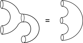
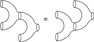
Figure 2: $(a)$: The composition $\eta\circ(*\otimes\mathrm{id})=\eta\circ(\mathrm{id}\otimes*):\mathcal{V}_{N,M}^{\otimes 3}\to R$ corresponds to gluing an in-boundary of an annulus and an out-boundary of a pant which is equivalent to a sphere with three in-boundaries. $(b)$: The associativity condition for $\mathcal{V}_{N,M}^{\otimes 3}\to\mathcal{V}_{N,M}$ means the equivalence of two different gluing of two pants .

First we introduce $\eta^{\mu\nu}$ defined by

$$\eta^{\mu\nu}:=\sum_{\alpha\in\mathcal{P}_{N,M}}\frac{\Pi(y_{\alpha})^{2}}{\Pi(t_{\mu})\Pi(t_{\nu})}\frac{G_{\mu^{\vee}}(y_{\alpha}|\ominus t^{\prime})G_{\nu^{\vee}}(y_{\alpha}|\ominus t^{\prime})}{{\sf e}(y_{\alpha},y_{\alpha})}.$$ (2.61)

Then $\eta^{\mu\nu}$ is the inverse of $\eta_{\mu\nu}$, since these satisfy the relation $\sum_{\nu\in\mathcal{P}_{N,M}}\eta_{\mu\nu}\eta^{\nu\rho}=\delta^{\rho}_{\mu}$ which follows from the formula (2.45). We introduce the pictorial expression of the product $*$, the bilinear form $\eta$, and identity $|v_{\emptyset}\rangle$ as depicted in Figure 1. The inverse of $\eta$ is associated to an annulus with two out-boundaries. A contraction of an upper index and a lower index corresponds to a gluing of an in-boundary and an out-boundary (See Figure 3).

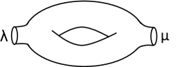
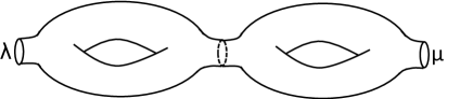
Figure 3: $(a)$: We associate $C^{(1)\mu}_{\quad\lambda}$ to a genus one surface with an in-boundary and out-boundary. $\lambda$ at the in-boundary and $\mu$ at the out-boundary denote the lower and upper indices of $C^{(1)\mu}_{\quad\lambda}$, respectively. $(b)$: A contraction $\sum_{\nu}C^{(1)\mu}_{\quad\nu}C^{(1)\nu}_{\quad\lambda}$ corresponds to gluing two genus one surface with an in-boundary and out-boundary, which is a genus two surface with an in-boundary and out-boundary and is expressed by $C^{(2)\mu}_{\quad\lambda}$.

We introduce $C^{(g)\mu_{1}\cdots\mu_{l}}_{\quad\lambda_{1}\cdots\lambda_{n}}(q,t,\beta)$ defined by contractions of $C^{\lambda_{1}}_{\lambda_{2}\lambda_{3}}$’s, $\eta_{\mu_{1}\mu_{2}}$’s, and $\eta^{\nu_{1}\nu_{2}}$’s which corresponds to the genus $g$ surface with $n$ in-boundaries and $l$ out-boundaries. $\lambda_{i}$ is assigned to an in-boundary and $\mu_{i}$ is assigned to an out-boundary. For example, $g=1,2$ with $n=l=1$ are depicted in Figure 3.

Note that $C^{(g)\mu_{1}\cdots\mu_{l}}_{\quad\lambda_{1}\cdots\lambda_{n}}$ satisfies the following properties

$$C^{(0)\lambda}_{\quad\mu\nu} =C^{\lambda}_{\mu\nu},\quad C^{(0)}_{\quad\mu\nu}=\eta_{\mu\nu},\quad C^{(0)\mu\nu}=\eta^{\mu\nu},$$ (2.62)

$$C^{(g)\mu_{1}\cdots\mu_{l-1}\emptyset}_{\quad\lambda_{1}\cdots\lambda_{n}} =C^{(g)\mu_{1}\cdots\mu_{l-1}}_{\quad\lambda_{1}\cdots\lambda_{n}},$$ (2.63)

$$C^{(g)\mu_{1}\cdots\mu_{l}}_{\quad\lambda_{1}\cdots\lambda_{n-1}\emptyset} =C^{(g)\mu_{1}\cdots\mu_{l}}_{\quad\lambda_{1}\cdots\lambda_{n-1}},$$ (2.64)

$$C^{(g_{1}+g_{2})\mu_{1}\cdots\mu_{l_{1}+l_{2}}}_{\quad\quad\lambda_{1}\cdots\lambda_{n_{1}+n_{2}}} =\sum_{\nu_{1}\nu_{2}}C^{(g_{1})\mu_{1}\cdots\mu_{l_{1}}}_{\quad\lambda_{1}\cdots\lambda_{n_{1}}\nu_{1}}\eta^{\nu_{1}\nu_{2}}C^{(g_{2})\mu_{l_{1}+1}\cdots\mu_{l_{1}+l_{2}}}_{\quad\nu_{2}\lambda_{n_{1}+1}\cdots\lambda_{n_{1}+n_{2}}},$$ (2.65)

$$C^{(g_{1}+g_{2})\mu_{1}\cdots\mu_{l_{1}+l_{2}}}_{\quad\quad\lambda_{1}\cdots\lambda_{n_{1}+n_{2}}} =\sum_{\nu_{1}\nu_{2}}C^{(g_{1})\mu_{1}\cdots\mu_{l_{1}}\nu_{1}}_{\quad\lambda_{1}\cdots\lambda_{n_{1}}}\eta_{\nu_{1}\nu_{2}}C^{(g_{2})\nu_{2}\mu_{l_{1}+1}\cdots\mu_{l_{1}+l_{2}}}_{\quad\lambda_{n_{1}+1}\cdots\lambda_{n_{1}+n_{2}}}.$$ (2.66)

$C^{(1)\mu}_{\quad\lambda}$ is written in terms of Grothendieck polynomial as

$$C^{(1)\mu}_{\quad\lambda}(q,t,\beta) =\sum_{\nu_{1},\nu_{2}\nu_{3}\in\mathcal{P}_{N,M}}\eta^{\nu_{2}\nu_{3}}C^{\nu_{1}}_{\lambda\nu_{2}}C^{\mu}_{\nu_{1}\nu_{3}}$$

$$=\sum_{\alpha\in\mathcal{P}_{N,M}}\frac{\Pi(y_{\alpha})}{\Pi(t_{\mu})}{G_{\lambda}(y_{\alpha}|\ominus t)G_{\mu^{\vee}}(y_{\alpha}|\ominus t^{\prime})}.$$ (2.67)

Here we used (2.44). $C^{(g)\mu}_{\quad\lambda}$ is calculated by contracting upper and lower indices of $C^{(1)\mu}_{\quad\lambda}$ as

$${C}^{(g)\mu}_{\quad\lambda} =\sum_{\nu_{1},\cdots,\nu_{g-1}\in\mathcal{P}_{N,M}}C^{(1)\mu}_{\quad\nu_{1}}\left(\prod_{k=1}^{g-2}C^{(1)\nu_{k}}_{\quad\nu_{k+1}}\right)C^{(1)\nu_{g-1}}_{\quad\lambda}$$

$$=\sum_{{\alpha}\in\mathcal{P}_{N,M}}\frac{\Pi(y_{\alpha})}{\Pi(t_{\mu})}\frac{G_{\lambda}(y_{\alpha}|\ominus t)G_{\mu^{\vee}}(y_{\alpha}|\ominus t^{\prime})}{{\sf e}(y_{\alpha},y_{\alpha})^{1-g}}.$$ (2.68)

The genus $g$ Riemann surface corresponds to the contraction $\sum_{\mu\in\mathcal{P}_{N,M}}C^{(g)\mu}_{\quad\mu}$ given by

$$Z(\Sigma_{g}) :=\sum_{\mu\in\mathcal{P}_{N,M}}C^{(g)\mu}_{\quad\mu}=\sum_{\alpha\in\mathcal{P}_{M,N}}{\sf e}(y_{\alpha},y_{\alpha})^{g-1}.$$ (2.69)

Although we defined $Z(\Sigma_{g})$ in a particular basis $\{v_{\lambda}\}_{\lambda\in\mathcal{P}_{N,M}}$ of $\mathcal{V}_{N,M}$, $Z(\Sigma_{g})$ is independent of the choices of bases. $Z(\Sigma_{g})$ is sometimes called the genus $g$ partition function of 2d TQFT. In section 3, we will show $Z(\Sigma_{g})$ for $\beta=0$ agrees with a partition function of A-twisted GLSM on $\Sigma_{g}$ and, in section 4.1, we will show $Z(\Sigma_{g})$ for $\beta=-1$ agrees with the partition function (topologically twisted index) of a CS–matter theory on $S^{1}\times\Sigma_{g}$.

Next we express $C^{(g)}_{\mu_{1}\mu_{2}\cdots\mu_{n}}$ in terms of Grothendieck polynomials and the on-shell square norms. By using the relation (2.44), we obtain

$$C^{(0)}_{\lambda_{1}\lambda_{2}\cdots\lambda_{n}}(q,t,\beta) =\sum_{\nu_{1},\cdots,\nu_{n-2}\in\mathcal{P}_{N,M}}C^{\nu_{1}}_{\lambda_{1}\lambda_{2}}C^{\nu_{2}}_{\nu_{1}\lambda_{3}}C^{\nu_{3}}_{\nu_{2}\lambda_{4}}\cdots C^{\nu_{n-2}}_{\nu_{n-3}\lambda_{n-1}}C^{\emptyset}_{\nu_{n-2}\lambda_{n}}$$

$$=\sum_{\alpha\in\mathcal{P}_{M,N}}\frac{\prod_{l=1}^{n}G_{\lambda_{l}}(y_{\alpha}|\ominus t)}{{\sf e}({y}_{\alpha},{y}_{\alpha})}.$$ (2.70)

From (2.68) and (2.70), $C^{(g)}_{\lambda_{1}\lambda_{2}\cdots\lambda_{n}}$ is given by

$$C^{(g)}_{\lambda_{1}\lambda_{2}\cdots\lambda_{n}}(q,t,\beta) =\sum_{\nu\in\mathcal{P}_{N,M}}C^{(0)}_{\lambda_{1}\lambda_{2}\cdots\lambda_{n-1}\nu}C^{(g)\nu}_{\quad\lambda_{n}}$$

$$=\sum_{\alpha\in\mathcal{P}_{M,N}}\frac{\prod_{l=1}^{n}G_{\lambda_{l}}(y_{\alpha}|\ominus t)}{{\sf e}({y}_{\alpha},{y}_{\alpha})^{1-g}}.$$ (2.71)

We will show that $C^{(g)}_{\lambda_{1}\lambda_{2}\cdots\lambda_{n}}(q,t,\beta)$ is same as an $n$-point correlation function in A-twisted GLSM on $\Sigma_{g}$ for $\beta=0$ and an $n$-point correlation function in CS–matter theory on $S^{1}\times\Sigma_{g}$ for $\beta=-1$. We call (2.71) as a genus $g$ correlation function of 2d TQFT.

The level-rank duality (2.59) and (2.60) leads to the equality of $C^{(g)}_{\lambda_{1}\lambda_{2}\cdots\lambda_{n}}$ between $\mathcal{V}_{N,M}$ and $\mathcal{V}_{M-N,M}$:

$$C^{(g)}_{\lambda_{1}\lambda_{2}\cdots\lambda_{n}}(q,t,\beta) =C^{(g)}_{\lambda^{\prime}_{1}\lambda^{\prime}_{2}\cdots\lambda^{\prime}_{n}}(q,\ominus t^{\prime},\beta).$$ (2.72)

2.3 Determinant representation of the on-shell square norm

In order to relate the quantum $K$-ring with the inner product (2.52) to correlation functions and the algebra of supersymmetric Wilson loops in a supersymmetric Chern–Simons–matter theory, we have to express the on-shell inner product ${\sf e}(y_{\lambda},y_{\lambda})$ in (2.58) as a nice function of the Bethe roots $\{y_{\lambda}\}_{\lambda\in\mathcal{P}_{N,M}}$ and the inhomogeneous parameters $\{t_{i}\}_{i=1}^{M}$. It was shown in [29, 30] that the partition functions of $U(N)/U(N)$ gauged Wess-Zumino-Witten (WZW) model and its deformation (called gauged WZW–matter model) are written in terms of the determinant type formulas of the on-shell norms for the phase model and $q$-boson, respectively. Moreover the partition functions of the gauged WZW model and the gauged WZW-matter model on the Riemann surfaces agree with the partition functions of 2d TQFTs associated to the Frobenius algebras in [32, 33]. Motivated by these agreements between gauge theories and 2d TQFTs observed in [29, 30, 34, 35], we apply Izergin-Korepin method [36] and express the on-shell square norm by the determinant type formula. See also [37] for a review of derivation of the norm for the spin-$\frac{1}{2}$ XXZ spin chain. The derivation of determinant type formula for ${\sf e}(y_{\lambda},y_{\lambda})$ is parallel to that for the XXZ spin chain.

First we study the off-shell inner product between the Bethe vector and the dual Bethe vector for indeterminate variables $\{x\}:=\{x_{1},\cdots,x_{N}\}$ and $\{y\}=\{y_{1},\cdots,y_{N}\}$. Recall that the off-shell inner product is defined by

$$S_{N}(\{x\},\{y\}):=\langle 0|\prod_{a=1}^{N}{\sf C}(x_{a})\prod_{a=1}^{N}{\sf B}(y_{a})|0\rangle.$$ (2.73)

From (B.8) and (2.36), the most general form of (2.73) is expressed as

$$S_{N}(\{x\}|\{y\}) =\sum_{\alpha\cup\overline{\alpha}\atop\gamma\cup\overline{\gamma}}\prod_{j\in\gamma}{\sf a}(x_{j})\prod_{k\in\overline{\gamma}}{\sf d}(x_{k})\prod_{k\in\overline{\alpha}}{\sf a}(y_{k})\prod_{j\in\alpha}{\sf d}(y_{j})$$

$$\qquad\qquad\times{\sf K}_{N}(\{x\}_{\gamma},\{x\}_{\overline{\gamma}}|\{y\}_{\alpha},\{y\}_{\overline{\alpha}}).$$ (2.74)

Here $\{x\}_{\alpha}$ and $\{x\}_{\overline{\alpha}}$ are two disjoint subsets of $\{x\}$ with $\{x\}_{\alpha}\cup\{x\}_{\overline{\alpha}}=\{x\}$. $\{y\}_{\gamma}$ and $\{y\}_{\overline{\gamma}}$ are two disjoint subsets of $\{y\}$ with $\{y\}_{\gamma}\cup\{y\}_{\overline{\gamma}}=\{y\}$. The subsets $\{x\}_{\alpha}$, $\{x\}_{\overline{\alpha}}$, $\{y\}_{\gamma}$, and $\{y\}_{\overline{\gamma}}$ are ordered as $\{x\}_{\alpha}=\{x_{\alpha_{1}},\cdots,x_{\alpha_{n}}\}$, if $\alpha_{1}<\cdots<\alpha_{n}$ and so on. Note that ${\sf K}_{N}(\{x\}_{\gamma},\{x\}_{\overline{\gamma}}|\{y\}_{\alpha},\{y\}_{\overline{\alpha}})$ depends on the R-matrix (2.5), but is independent of the eigen values of ${\sf A}$ and ${\sf D}$ in the monodromy matrix. In the following evaluation of ${\sf K}_{N}(\{x\}_{\gamma},\{x\}_{\overline{\gamma}}|\{y\}_{\alpha},\{y\}_{\overline{\alpha}})$, we fix the partition $\alpha,\overline{\alpha}$ and $\gamma,\overline{\gamma}$.

The leading coefficient ${\sf K}_{N}(\{x\},\{y\})$ and the conjugate leading coefficient $\overline{{\sf K}}_{N}(\{x\},\{y\})$ are defined by

$${\sf K}_{N}(\{x\}|\{y\}):={\sf K}_{N}(\{x\}_{\gamma},\{x\}_{\overline{\gamma}}=\emptyset|\{y\}_{\alpha},\{y\}_{\overline{\alpha}}=\emptyset),$$ (2.75)

$$\overline{{\sf K}}_{N}(\{x\}|\{y\}):={\sf K}_{N}(\{x\}_{\gamma}=\emptyset,\{x\}_{\overline{\gamma}}|\{y\}_{\alpha}=\emptyset,\{y\}_{\overline{\alpha}}).$$ (2.76)

An important property is that ${\sf K}_{N}(\{x\}_{\gamma},\{x\}_{\overline{\gamma}}|\{y\}_{\alpha},\{y\}_{\overline{\alpha}})$ is expressed in terms of the leading and conjugate leading coefficients as follows.

$${\sf K}_{N}(\{x\}_{\gamma},\{x\}_{\overline{\gamma}}|\{y\}_{\alpha},\{y\}_{\overline{\alpha}}) =\prod_{a\in\alpha}\prod_{b\in\overline{\alpha}}g(y_{a},y_{b})\prod_{a\in\gamma}\prod_{b\in\overline{\gamma}}g(x_{a},x_{b})$$

$$\times{\sf K}_{n}(\{x\}_{\gamma}|\{y\}_{\alpha})\overline{{\sf K}}_{N-n}(\{x\}_{\overline{\gamma}}|\{y\}_{\overline{\alpha}}).$$ (2.77)

Here $g(x,y)$ is a coefficient in the RTT relation given by

$${\sf C}(x){\sf B}(y)=g(y,x)\left({\sf A}(x){\sf D}(y)-{\sf A}(y){\sf D}(x)\right),$$ (2.78)

with

$$g(y,x):=\frac{1}{x\ominus y}.$$ (2.79)

Then, it is enough to evaluate the leading and the conjugate leading coefficients to evaluate the off-shell inner product (2.74). Let us consider to evaluate the leading and the conjugate leading coefficients. From (2.78), we obtain

$${\sf C}(x_{N})\prod_{j=1}^{N}{\sf B}(y_{j})|0\rangle =\sum_{l=1}^{N}{\sf a}(x_{N}){\sf d}(y_{l})g(y_{l},x_{N})\left(\prod_{j=1\atop j\neq l}^{N}g(y_{j},x_{N})g(y_{l},y_{j})\right)\prod_{j=1\atop j\neq l}^{n}{\sf B}(y_{j})|0\rangle+\cdots$$ (2.80)

Here the ellipses denote the terms which are irrelevant to the evaluation of the leading coefficient. Multiplying (2.80) by $\langle 0|\prod_{i=1}^{N-1}{\sf C}(x_{i})$ , we find the leading coefficients satisfy the following recurrence relation.

$${\sf K}_{N}(\{x\}|\{y\}) =\sum_{l=1}^{N}g(y_{l},x_{N})\left(\prod_{a=1\atop a\neq l}^{N}g(y_{a},x_{N})g(y_{l},y_{a})\right){\sf K}_{N-1}(\{x\neq x_{N}\}|\{y\neq y_{l}\}).$$ (2.81)

In a similar way, the recurrence relation for the conjugate leading coefficients is given by

$$\overline{{\sf K}}_{N}(\{x\}|\{y\}) =-\sum_{l=1}^{N}g(y_{l},x_{N})\left(\prod_{a=1\atop a\neq l}^{N}g(x_{N},y_{a})g(y_{a},y_{l})\right)\overline{{\sf K}}_{N-1}(\{x\neq x_{N}\}|\{y\neq y_{l}\}).$$ (2.82)

With the following initial condition

$${\sf K}_{1}(\{x\}|\{y\})=\frac{1+\beta y}{x-y},\quad\overline{{\sf K}}_{1}(\{x\}|\{y\})=\frac{1+\beta y}{y-x},$$ (2.83)

the recurrence relations (2.81) and (2.82) are solved as

$${\sf K}_{N}(\{x\}|\{y\}) =\frac{\prod_{b=1}^{N}(1+\beta y_{b})^{N+1}}{\prod_{a>b}^{N}(x_{b}-x_{a})(y_{a}-y_{b})}\det_{k,j}{\sf t}(x_{k},y_{j}),$$ (2.84)

$$\overline{{\sf K}}_{N}(\{x\}|\{y\}) =\frac{\prod_{a=1}^{N}(1+\beta y_{a})(1+\beta x_{a})^{N}}{\prod_{a>b}^{N}(x_{b}-x_{a})(y_{a}-y_{b})}\det_{j,k}{\sf t}(y_{j},x_{k}),$$ (2.85)

where ${\sf t}(x,y)$ is defined by

$${\sf t}(x,y):=\frac{1}{(x-y){(1+\beta y)}}.$$ (2.86)

$\mathrm{det}_{j,k}$ denotes the determinant with respect to indices $j,k$. We show that (2.84) satisfies the recurrence relation (2.81) as follows. By adding the $j$-th row of the matrix ${\sf t}(x_{j},y_{k})$ multiplied by $u_{j}/u_{N}$ with $j=1,\cdots,N-1$ to the $N$-th row of ${\sf t}(x_{j},y_{k})$, we obtain the following relation between determinants for ${\sf t}(x_{j},y_{k})$:

$$\det_{j,k}{\sf t}(x_{j},y_{k}) =\frac{1}{u_{N}}\sum_{l=1}^{N}(-1)^{N+l}G_{l}\det_{j,k\atop j\neq Nk\neq l}{\sf t}(x_{j},y_{k}),$$ (2.87)

where $G_{l}$ is defined by $G_{l}:=\sum_{k=1}^{N}u_{k}{\sf t}(x_{k},y_{l})$. If $u_{k}$ is chosen as

$$u_{k}=\frac{\prod_{a=1}^{N}(x_{k}-y_{a})}{\prod_{a=1\atop a\neq k}^{N}(x_{k}-x_{a})},$$ (2.88)

then $G_{l}$ satisfies the following identity:

$$G_{l}=\frac{1}{1+\beta y_{l}}.$$ (2.89)

To show (2.89), we consider the integral:

$$I=\frac{1}{1+\beta y_{l}}\oint_{\Gamma}\frac{dz}{2\pi{\rm i}}\frac{\prod_{a=1\atop a\neq l}^{N}(z-y_{a})}{\prod_{a=1}^{N}(z-x_{a})}\,.$$ (2.90)

Here the contour encloses all the poles of the integrand; $z=\infty,x_{1},\cdots,x_{N}$. The residues at $z=\infty$ and $z=x_{1},\cdots,x_{N}$ are evaluated as

$$\frac{1}{1+\beta y_{l}}\oint_{z=\infty}\frac{dz}{2\pi{\rm i}}\frac{\prod_{a=1\atop a\neq l}^{N}(z-y_{a})}{\prod_{a=1}^{N}(z-x_{a})} =-\frac{1}{1+\beta y_{l}}\,,$$

$$\frac{1}{1+\beta y_{l}}\sum_{k=1}^{N}\oint_{z=x_{k}}\frac{dz}{2\pi{\rm i}}\frac{\prod_{a=1\atop a\neq l}^{N}(z-y_{a})}{\prod_{a=1}^{N}(z-x_{a})} =G_{l}\,.$$ (2.91)

Since $I=0$, we obtain (2.89)

From (2.87) with the identity (2.89), we find that (2.84) satisfies the recurrence relation (2.81). Thus the right hand side of (2.84) is the leading coefficient. In a similar way, we can show that (2.85) satisfies the recurrence relation for $\bar{K}_{N}$.

Substituting the solutions of the recurrence relations to (2.74), we have

$$S_{N}(\{x\}|\{y\}) =\left(\prod_{b=1}^{N}(1+\beta y_{b})\right)\left(\prod^{N}_{a>b}(x_{b}-x_{a})^{-1}(y_{a}-y_{b})^{-1}\right)$$

$$\times\sum_{\alpha\cup\overline{\alpha}\atop\gamma\cup\overline{\gamma}}(-1)^{P_{\alpha}+P_{\gamma}}\prod_{j\in\gamma}{\sf a}(x_{j})\prod_{k\in\overline{\gamma}}{\sf d}(x_{k})\prod_{k\in\overline{\alpha}}{\sf a}(y_{k})\prod_{j\in\alpha}{\sf d}(y_{j})\det_{j\in\alpha\atop k\in\gamma}{\sf t}(x_{k},y_{j})\det_{j\in\overline{\alpha}\atop k\in\overline{\gamma}}{\sf t}(y_{j},x_{k})$$

$$\times\prod_{a\in{\alpha}}\prod_{b\in{\gamma}}h(y_{a},x_{b})\prod_{a\in\overline{\alpha}}\prod_{b\in\overline{\gamma}}h(x_{b},y_{a})\prod_{a\in\alpha}\prod_{b\in\overline{\alpha}}h(y_{a},y_{b})\prod_{a\in\gamma}\prod_{b\in\overline{\gamma}}h(x_{b},x_{a})$$ (2.92)

with

$$h(x,y):=g(x,y)(y-x)=1+\beta x.$$ (2.93)

$P_{\alpha}$ is the parity of the partition $(\alpha_{1},\cdots,\alpha_{n},\bar{\alpha}_{1},\cdots,\bar{\alpha}_{N-n})$, defined as 0 (resp. 1) when $(\alpha_{1},\cdots,\bar{\alpha}_{N-n})$ is an even (resp. odd) permutation of $(1,2,\cdots,N)$. Now assume that $\{y\}$ in (2.92) is a Bethe root. By using the Bethe ansatz equation and the identity

$$\det_{j,k}\left(U(y_{j},x_{k})+V(y_{j},x_{k})\right)=\sum_{\alpha\cup\bar{\alpha}\atop\gamma\cup\bar{\gamma}}(-1)^{P_{\alpha}+P_{\gamma}}\det_{j\in\alpha\atop k\in\gamma}U(y_{j},x_{k})\det_{j\in\bar{\alpha}\atop k\in\bar{\gamma}}V(y_{j},x_{k})\,,$$ (2.94)

we obtain the following expression of the square norm after some calculation:

$$S_{N}(\{x\}|\{y\}) =\frac{\prod_{b=1}^{N}(1+\beta y_{b})}{\prod_{a>b}^{N}(x_{b}-x_{a})(y_{a}-y_{b})}\det_{a,b}\Omega_{q}(y_{a},x_{b}),$$ (2.95)

where

$$\Omega_{q}(y_{a},x_{b}) :={\sf a}(x_{b}){\sf t}(x_{b},y_{a})\prod_{c=1}^{N}(1+\beta y_{c})-(-1)^{N}q\,{\sf t}(y_{a},x_{b})(1+\beta x_{b})^{N}.$$ (2.96)

Finally, by taking limit $x_{a}\to y_{a}$, we obtain the determinant formula of the on-shell square norm given by

$${\sf e}(y,y) =\frac{\prod_{i=1}^{M}\prod_{a=1}^{N}(y_{a}-t_{i})}{\prod_{i=1}^{M}(1+\beta t_{i})^{N}}\frac{\prod_{a=1}^{N}(1+\beta y_{a})^{N-1}}{\prod_{a>b}^{N}(y_{a}-y_{b})^{2}}\det_{a,b}\left[\delta_{a,b}\left(\sum_{i=1}^{M}\frac{1+\beta y_{a}}{y_{a}-t_{i}}-N\beta\right)+\beta\right].$$ (2.97)

We are interseted in the expression of ${\sf e}(y,y)$ with slices $\beta=-1,0$. When $\beta=0$, the inverse of ${\sf e}(y,y)$ is given by

$${\sf e}(y,y)^{-1}= \frac{\prod_{a>b}^{N}(y_{a}-y_{b})^{2}}{\prod_{i=1}^{M}\prod_{a=1}^{N}(y_{a}-t_{i})}\prod_{a=1}^{N}\left[\left(\sum_{i=1}^{M}\frac{1}{y_{a}-t_{i}}\right)\right]^{-1}.$$ (2.98)

When $\beta=-1$, the inverse of ${\sf e}(y,y)$ is given by

$${\sf e}(y,y)^{-1} =\frac{\prod_{i=1}^{M}(1-t_{i})^{N}\prod_{a>b}^{N}(y_{a}-y_{b})^{2}}{\prod_{a=1}^{N}(1-y_{a})^{N-1}\prod_{i=1}^{M}(y_{a}-t_{i})}\det_{a,b}\left[\delta_{a,b}\left(\sum_{i=1}^{M}\frac{1-y_{a}}{y_{a}-t_{i}}+N\right)-1\right]^{-1}.$$ (2.99)

3 2d A-twisted GLSM and quantum coholomogy of Grassmannian

In this section we study a 2d A-twisted GLSM on the genus $g$ Riemann surface $\Sigma_{g}$. The gauge group of GLSM is taken to be $G=U(N)$ and the $M$ chiral multiplets are in the fundamental representation of $U(N)$ with $M>N$. If we put the GLSM on $\mathbb{R}^{2}$, the Higgs branch vacua is a Grassmannian $\text{Gr}(N,M)$ in the positive Fayet–Iliopoulos (FI) parameter region.

The motivation of this section is threefold. The first is to establish Bethe/Gauge correspondence between the algebraic Bethe ansatz for $\beta=0$ and the 2d $U(N)$ GLSM with $M$ fundamental chiral multiplets. As far as we know, Bethe/Gauge correspondence for A-twisted GLSM for $M$ fundamental chiral multiplet has not been studied. The second is to explain how the expression (2.58) of three-point Gromov–Witten invariants appears in A-twisted 2d GLSM on $S^{2}$ . The third is to show that the correlation functions of A-twisted 2d GLSM on higher-genus Riemann surfaces agree with those of 2d TQFT associated with the Frobenius algebra. This suggests that these correlation functions are quasimap invariants with fixed domains.

3.1 A-twisted GLSM on $S^{2}$ and genus zero quasimap invariants

First we consider the genus zero case. In terms of supersymmetric localization formula [8], the $n$-point correlation functions of gauge invariant functions $\widehat{\mathcal{O}}_{\text{2d}.l}$ of the $U(N)$ vector multiplet scalar in the A-twisted GLSM on $S^{2}$ is written as the following form:

$$\langle\prod_{l=1}^{n}\widehat{\mathcal{O}}_{\text{2d}.l}\rangle_{S^{2}} =\frac{1}{N!}\sum_{a=1}^{N}\sum_{k_{a}=0}^{\infty}\oint\prod_{a=1}^{N}\frac{d\sigma_{a}}{2\pi{\rm i}}\left(\prod_{l=1}^{n}\mathcal{O}_{\text{2d}.l}(\sigma,m)\right)Z_{\text{FI}}Z^{(0)}_{\text{2d.vec}}(\sigma,k)Z^{(0)}_{\text{2d.chi}}(\sigma,k)$$

$$=\frac{1}{N!}\sum_{a=1}^{N}\sum_{k_{a}=0}^{\infty}\oint\prod_{a=1}^{N}\frac{d\sigma_{a}}{2\pi{\rm i}}\left(\prod_{l=1}^{n}\mathcal{O}_{\text{2d}.l}(\sigma,m)\right)$$

$$\qquad\qquad\times((-1)^{N-1}q)^{\sum_{a=1}^{N}k_{a}}\frac{\prod_{1\leq a<b\leq N}(\sigma_{a}-\sigma_{b})^{2}}{\prod_{i=1}^{M}\prod_{a=1}^{N}\left(\sigma_{a}-m_{i}\right)^{k_{a}+1-r}}.$$ (3.1)

Here the residues in (3.1) are evaluated at $\sigma_{a}=m_{i_{a}}$ with $a=1,\cdots,N$ and $i_{a}=1,\cdots,M$. $\{\sigma_{a}\}_{a=1}^{N}$ is the saddle point value of $\mathfrak{u}(N)\otimes\mathbb{C}$ valued scalar $\sigma$ in the $U(N)$ vector multiplet:

$$\sigma|_{\text{saddle point}}=:\mathrm{diag}(\sigma_{1},\cdots,\sigma_{N}).$$ (3.2)

$\{k_{a}\}_{a=1}^{N}$ is magnetic charges of gauge fields for the maximal torus of $U(N)$. $Z_{\text{FI}}$ is the contribution from the saddle point value of the FI term and theta term which is given by

$$Z_{\text{FI}}=e^{-S_{\text{FI}}}|_{\text{saddle point}}=q^{\sum_{a=1}^{N}k_{a}},$$ (3.3)

where $S_{\text{FI}}$ is the actions of FI-term and theta-term. $\log q=2\pi{\rm i}\theta-\xi$ is the holomorphic combination of the FI parameter $\xi$ and the theta angle $\theta$. $q$ is identified with the quantum parameter or equivalently the parameter of twisted boundary condition in the algebraic Bethe ansatz. $Z^{(0)}_{\text{2d.vec}}(\sigma,k)$ and $Z^{(0)}_{\text{2d.chi}}(\sigma,k)$ are the one-loop determinant of the 2d A-twisted super Yang-Mills action on $S^{2}$ and the one-loop determinant of the $M$ chiral multiplets on $S^{2}$ given by

$$Z^{(0)}_{\text{2d.vec}}(\sigma,k) =(-1)^{(N-1)\sum_{a=1}^{N}k_{a}}\prod_{1\leq a<b\leq N}(\sigma_{a}-\sigma_{b})^{2},$$ (3.4)

$$Z^{(0)}_{\text{2d.chi}}(\sigma,k) =\prod_{i=1}^{M}\prod_{a=1}^{N}\left(\frac{1}{\sigma_{a}-m_{i}}\right)^{k_{a}+1-r}.$$ (3.5)

Here $m_{i}$ is the twisted mass of the $i$-th chiral multiplet and $r\in\mathbb{Z}_{\geq 0}$ is a vector type $U(1)$ R-charge.

$\widehat{\mathcal{O}}_{\text{2d}.l}$ is a gauge invariant operator consisting of $\sigma$. $\mathcal{O}_{\text{2d}.l}(\sigma)$ in the right hand side in (3.1) expresses the saddle point value of $\widehat{\mathcal{O}}_{\text{2d}.l}$ which is a symmetric polynomial of $\{\sigma_{a}\}_{a=1}^{N}$ and is a polynomial of the mass parameters $\{m_{i}\}_{i=1}^{M}$. For example, let us consider the saddle point value of a gauge invariant operator $\mathrm{Tr}\sigma$. Here $\mathrm{Tr}$ is the trace of a $N\times N$ matrix. The saddle point value is given by

$$\mathrm{Tr}\sigma|_{\text{saddle point}}=\mathrm{Tr}\,\mathrm{diag}(\sigma_{1},\cdots,\sigma_{N})=\sum_{a=1}^{N}\sigma_{a}.$$ (3.6)

Note that the A-twisted GLSM is topologically twisted theory and the correlation function of vector multiplet scalar ($\mathcal{Q}$-closed operator) are independent of the coordinates of $S^{2}$ on which the operators are inserted. Then an $n$-point correlation function have the same value of the expectation value of the single operator consisting of the product of $n$-operators inserted on a point on $S^{2}$.

For any given symmetric polynomial $f(\sigma_{1},\cdots,\sigma_{N})$ of $\sigma_{1},\cdots,\sigma_{N}$, there exists a gauge invariant operator of $\sigma$ whose saddle value is given by $f(\sigma_{1},\cdots,\sigma_{N})$. We may define $\hat{s}_{\lambda}$ by the gauge invariant operator of $\sigma$ including $m_{i}$, whose saddle point is given by a factorial Schur polynomial $s_{\lambda}(\sigma|m)$. It is enough to consider the correlation functions of $\hat{s}_{\lambda}$, since $\{s_{\lambda}(\sigma|m)\}_{\lambda\in\mathcal{P}_{N,M}}$ generate the symmetric polynomials of $\sigma_{1},\cdots,\sigma_{N}$.

The algebra of scalars in the vector multiplet (twisted chiral ring) is given by

$$\langle\cdots\widehat{\mathcal{O}}_{\mathrm{2d.}i}\widehat{\mathcal{O}}_{\mathrm{2d.}j}\cdots\rangle_{S^{2}}=\langle\cdots\sum_{k}N^{\prime k}_{ij}\,\widehat{\mathcal{O}}_{\mathrm{2d.}k}\cdots\rangle_{S^{2}}.$$ (3.7)

Here ellipses denote the arbitrary insertions of gauge invariant combination of vector multiplet scalar and $N^{\prime k}_{ij}$’s are the coefficients of OPEs.

We remark on properties of the algebra of scalars. The $\mathcal{Q}$-exact terms in the correlation functions vanish and do not contribute to the OPEs. If there exist a basis of the algebra of vector multiplet scalars such that the coefficients $N^{\prime k}_{ij}$ agree with the structure constants $C^{\lambda}_{\mu\nu}$ of the quantum cohomology, then the algebra of vector multiplet scalar is isomorphic to the quantum cohomology of Grassmannian $\mathrm{Gr}(N,M)$. When we regard A-twisted GLSM as a Frobenius algebra, Taking the expectation values of $\widehat{\mathcal{O}}_{\text{2d}.l}$ correspond to a Frobenius bilinear form and a choice of R-charges $r$ corresponds to a choice of Frobenius bilinear form. Although the expectation values depend on the R-charge, The coefficients of OPE of $\widehat{\mathcal{O}}_{\text{2d}.l}$, i.e., the structure constants are independent of $r$, we will show this later. We will choose a particular integer of R-charge $r$ to give identification with the Frobenius algebra with $\beta=0$.

It is shown in [10] that (3.1) with $r=0$ is the generating function of genus zero degree-$k$ ($k:=k_{1}+\cdots+k_{N}$) quasimap invariants, which imply that the three point function correlation functions of factorial Schur polynomials agrees with the genus zero three points $T$-equivariant Gromov–Witten invariants of Schubert classes $[X_{\lambda}],[X_{\mu}],$ and $[X_{\nu}]$ of $\mathrm{Gr}(N,M)$:

$$\langle\hat{s}_{\lambda}\hat{s}_{\mu}\hat{s}_{\nu}\rangle_{S^{2}} =C^{(0)}_{\lambda\mu\nu}(q,t,\beta=0).$$ (3.8)

We show (3.8) as follows. We first perform sums of $\{k_{a}\}_{a=1}^{N}$ in (3.1) and deform the integration contours. Then we obtain the following expression of $n$-point correlation function:

$$\langle\prod_{l=1}^{n}\hat{s}_{\lambda_{l}}\rangle_{S^{2}} =\frac{1}{N!}\oint\prod_{a=1}^{N}\frac{d\sigma_{a}}{2\pi{\rm i}}\left(\prod_{l=1}^{n}s_{\lambda_{l}}(\sigma|m)\right)\frac{Z^{(0)}_{\text{2d.vec}}(\sigma,k=0)Z^{(0)}_{\text{2d.chi}}(\sigma,k=0)}{\prod_{a=1}^{N}(1-\exp\left({\partial_{\sigma_{a}}W_{\text{2d.eff}}}\right))}$$

$$=\sum_{\sigma}\left(\prod_{l=1}^{n}s_{\lambda_{l}}(\sigma|m)\right)Z^{(0)}_{\text{2d.vec}}(\sigma,0)Z^{(0)}_{\text{2d.chi}}(\sigma,0)\left[\det_{a,b}\left(\frac{\partial^{2}W_{\text{2d.eff}}}{\partial\sigma_{a}\partial\sigma_{b}}\right)\right]^{-1}$$

$$=\sum_{\sigma}\left(\prod_{l=1}^{n}s_{\lambda_{l}}(\sigma|m)\right)\frac{\prod_{a<b}(\sigma_{a}-\sigma_{b})^{2}}{\prod_{i=1}^{M}\prod_{a=1}^{N}(\sigma_{a}-m_{i})^{1-r}}\prod_{a=1}^{N}\left(\sum_{i=1}^{M}\frac{1}{\sigma_{a}-m_{i}}\right)^{-1}.$$ (3.9)

Here $W_{\text{2d.eff}}$ is the effective twisted superpotential defined by

$$W_{\text{2d.eff}} :=\left(\log q+\pi{\rm i}(N-1)\right)\sum_{a=1}^{N}\sigma_{a}-\sum_{i=1}^{M}\sum_{a=1}^{N}(\sigma_{a}-m_{i})\left[\log(\sigma_{a}-m_{i})-1\right].$$ (3.10)

From the first to the second line in (3.9), the residues are evaluated at roots of the saddle point equations of the twisted superpotential; $\exp\left(\partial_{\sigma_{a}}W_{\mathrm{2d.eff}}\right)=1,a=1,\cdots,N$.

$$\exp\left({\partial_{\sigma_{a}}W_{\text{2d.eff}}}\right)=1\Leftrightarrow\prod_{i=1}^{N}(\sigma_{a}-m_{i})=(-1)^{N-1}q,\quad a=1,\cdots,N.$$ (3.11)

with $\sigma_{a}\neq\sigma_{b}$ for $a\neq b$ and up to the permutations of $\sigma_{1},\cdots,\sigma_{N}$. When $N=1$, (3.11) agrees with the ring relation of $QH_{T}(\mathbb{P}^{M-1})$. The sum $\sum_{\sigma}$ runs over the solutions of the saddle point equation of twisted superpotential. We find that the saddle point equation (3.11) is same as the Bethe ansatz equation (2.38) for $\beta=0$ with the following identification of variables between the GLSM and the Bethe ansatz (2.38).

$$\sigma_{a}\equiv y_{a},\quad m_{i}\equiv t_{i},\quad\text{for }\beta=0.$$ (3.12)

In this article a symbol ”$\equiv$” is used to express identifications of variables between two different theories.

From the determinant formula of on-shell square norm (2.98), if we choose $r=0$, (3.9) perfectly agrees with the genus zero correlation functions (2.70) for $\beta=0$ obtained by gluing the genus zero three point functions, i.e., the axiom of 2d TQFT.

$$\langle\prod_{l=1}^{n}\hat{s}_{\lambda_{l}}\rangle_{S^{2}} =C^{(0)}_{\lambda_{1}\lambda_{2}\cdots\lambda_{n}}(q,t,\beta=0)\quad\text{for }r=0.$$ (3.13)

Then we obtained the two equivalent expressions of the genus zero three point Gromov–Witten invariants of $\mathrm{Gr}(N,M)$ given by

$$\langle\prod_{l=1}^{3}\hat{s}_{\lambda_{i}}\rangle_{S^{2}} =\frac{1}{N!}\sum_{a=1}^{N}\sum_{k_{a}=0}^{\infty}\oint\prod_{a=1}^{N}\frac{d\sigma_{a}}{2\pi{\rm i}}\left(\prod_{l=1}^{3}s_{\lambda_{l}}(\sigma|t)\right)((-1)^{N-1}q)^{\sum_{a=1}^{N}k_{a}}\frac{\prod_{1\leq a<b\leq N}(\sigma_{a}-\sigma_{b})^{2}}{\prod_{i=1}^{M}\prod_{a=1}^{N}(\sigma_{a}-m_{i})^{k_{a}+1}}$$ (3.14)

$$=\sum_{\sigma}\left(\prod_{l=1}^{3}s_{\lambda_{l}}(\sigma|t)\right)\frac{\prod_{a<b}(\sigma_{a}-\sigma_{b})^{2}}{\prod_{i=1}^{M}\prod_{a=1}^{N}(\sigma_{a}-m_{i})}\prod_{a=1}^{N}\left(\sum_{i=1}^{M}\frac{1}{\sigma_{a}-m_{i}}\right)^{-1}.$$ (3.15)

Here the expression of the right hand side in the first line is same as the generating function of quasimap invariants and the expression in the second line is the equivariant version of genus zero Intriligator–Vafa formula. Note that three point functions in the quasimaps gives genus zero three point Gromov–Witten invariants. When $r=0$, the residues for $q^{k}$ with $k\geq 1$ in the two point functions $\langle\hat{s}_{\mu}\hat{s}_{\nu}\rangle_{S^{2}}$ in the GLSM with $\mu,\nu\in\mathcal{P}_{N,M}$ vanish and the two point functions agree with the equivariant integral of Schubert classes $[X_{\mu}],[X_{\nu}]\in H^{*}_{T}(\mathrm{Gr}(N,M))$ as

$$\langle\hat{s}_{\mu}\hat{s}_{\nu}\rangle_{S^{2}} =\frac{1}{N!}\sum_{i_{1},\cdots,i_{N}=1}^{M}\oint_{\sigma_{a}=m_{i_{a}}}\prod_{a=1}^{N}\frac{d\sigma_{a}}{2\pi{\rm i}}s_{\mu}(\sigma|t)s_{\nu}(\sigma|t)\frac{\prod_{1\leq a<b\leq N}(\sigma_{a}-\sigma_{b})^{2}}{\prod_{i=1}^{M}\prod_{a=1}^{N}(\sigma_{a}-m_{i})}$$

$$=\int_{\mathrm{Gr}(N,M)}^{T}[X_{\mu}]\cup[X_{\nu}].$$ (3.16)

Since the saddle point equations is independent of the R-charge $r$, the structure constants of the algebra of $\hat{\mathcal{O}}_{\text{2d}}$ in the correlation functions are independent of the R-charge. This can been seen as follows. From the saddle point equation (3.11), the genus zero $n$-correlation function with $r$ is related to that with $r=0$ as

$$\langle\prod_{l=1}^{n}\hat{s}_{\lambda_{l}}\rangle_{S^{2},r}=\langle\prod_{i=1}^{M}\prod_{a=1}^{N}(\sigma_{a}-m_{i})^{r}\prod_{l=1}^{n}\hat{s}_{\lambda_{l}}\rangle_{S^{2},r=0}=((-1)^{N-1}q)^{Nr}\langle\prod_{l=1}^{n}\hat{s}_{\lambda_{l}}\rangle_{S^{2},r=0}$$ (3.17)

Here $\langle\cdots\rangle_{S^{2},r}$ denotes the correlation functions on $S^{2}$ with R-charge $r$. Then we find that the R-charge dependence is canceled out in the structure constants $C^{\lambda}_{\mu\nu}=\eta^{\lambda\rho}C^{(0)}_{\rho\mu\nu}$.

3.2 A-twisted GLSM on the general Riemann surfaces and 2d TQFT

Next we consider A-twisted GLSM on $\Sigma_{g}$ and show that the correlation functions of A-twisted GLSM agree with (2.71). In terms of the supersymmetric localization computation [23], an $n$-point correlation function on $\Sigma_{g}$ is written as

$$\langle\prod_{l=1}^{n}\widehat{\mathcal{O}}_{\text{2d}.l}\rangle_{\Sigma_{g}} =\frac{1}{N!}\oint\prod_{a=1}^{N}\frac{d\sigma_{a}}{2\pi{\rm i}}\sum_{a=1}^{N}\sum_{k_{a}=0}^{\infty}\left(\prod_{l=1}^{n}\mathcal{O}_{\text{2d}.l}(\sigma,m)\right)$$

$$\qquad\times Z_{\text{FI}}Z^{(g)}_{\text{2d.vec}}(\sigma,k)Z^{(g)}_{\text{2d.chi}}(\sigma,k)\left[\det_{a,b}\left(\frac{\partial^{2}W_{\text{2d.eff}}}{\partial\sigma_{a}\partial\sigma_{b}}\right)\right]^{g}.$$ (3.18)

Here the one-loop determinants for genus $g$ case are given by

$$Z^{(g)}_{\text{2d.vec}}(\sigma,k) =(-1)^{(N-1)\sum_{a=1}^{N}k_{a}}\prod_{1\leq a<b\leq N}(\sigma_{a}-\sigma_{b})^{2-2g},$$ (3.19)

$$Z^{(g)}_{\text{2d.chi}}(\sigma,k) =\prod_{i=1}^{M}\prod_{a=1}^{N}\left(\frac{1}{\sigma_{a}-m_{i}}\right)^{k_{a}+(1-r)(1-g)}.$$ (3.20)

When $g=0$, the formula is same as the localization formula on $S^{2}$ (3.1). We comment on the contour integrals in (3.1), (3.2). When $g=0$, in the order by order residue computations in the power of $q$, the contour integrals are determined by Jeffrey–Kirwan (JK) residues [39]. As we have seen in the previous section, we have two expressions (3.14) and (3.15) of the genus zero correlation functions in the A-twisted GLSM, both of them give the same result. In the derivation of the JK residue in supersymmetric localization, it is required that the singular hyperplane arrangement is projective, for example see [40]. When $g>1$, the one-loop determinant of the vector multiplet of non-abelian gauge group ($N\geq 2$) violates the projective condition and the order by order residue operations are not well-defined. We first perform the sums and obtain the following expression of the correlation function

$$\langle\prod_{l=1}^{n}\hat{s}_{\lambda_{l}}\rangle_{\Sigma_{g}} =\frac{1}{N!}\oint\prod_{a=1}^{N}\frac{d\sigma_{a}}{2\pi{\rm i}}\left(\prod_{l=1}^{n}{s}_{\lambda_{l}}(\sigma|m)\right)Z^{(g)}_{\text{2d.vec}}(\sigma,0)Z^{(g)}_{\text{2d.chi}}(\sigma,0)\frac{\left[\det_{a,b}\left(\partial_{\sigma_{a}}\partial_{\sigma_{b}}W_{\text{2d.eff}}\right)\right]^{g}}{\prod_{a=1}^{N}(1-\exp\left({\partial_{\sigma_{a}}W_{\text{2d.eff}}}\right))}$$ (3.21)

$$=\sum_{\sigma}\left(\prod_{l=1}^{n}{s}_{\lambda_{l}}(\sigma|m)\right)Z^{(g)}_{\text{2d.vec}}(\sigma,0)Z^{(g)}_{\text{2d.chi}}(\sigma,0)\left[\det_{a,b}\left(\frac{\partial^{2}W_{\text{2d.eff}}}{\partial\sigma_{a}\partial\sigma_{b}}\right)\right]^{g-1}$$ (3.22)

$$=\sum_{\sigma}\left(\prod_{l=1}^{n}{s}_{\lambda_{l}}(\sigma|m)\right)\left(\frac{\prod_{a<b}(\sigma_{a}-\sigma_{b})^{2}}{\prod_{i=1}^{M}\prod_{a=1}^{N}(\sigma_{a}-m_{i})^{1-r}}\prod_{a=1}^{N}\left(\sum_{i=1}^{M}\frac{1}{\sigma_{a}-m_{i}}\right)^{-1}\right)^{(1-g)}.$$ (3.23)

Again, if we choose $r=0$, (3.23) perfectly agrees with the correlation function on a genus $g$ correlation function obtained from the axiom of 2d TQFT;

$$\langle\prod_{l=1}^{n}\hat{s}_{\lambda_{l}}\rangle_{\Sigma_{g}}=C^{(g)}_{\lambda_{1}\lambda_{2}\cdots\lambda_{n}}(q,t,\beta=0)\quad\text{for }r=0.$$ (3.24)

In particular the partition function of the A-twisted GLSM with $r=0$ on $\Sigma_{g}$ agrees with the genus $g$ partition function of 2 TQFT with $\beta=0$;

$$\langle 1\rangle_{\Sigma_{g}}=\sum_{\lambda\in\mathcal{P}_{N,M}}{\sf e}(y_{\lambda},y_{\lambda})^{g-1}=Z(\Sigma_{g})\quad\text{for }\beta=0.$$ (3.25)

When $r=0$ and $m=0$, (3.23) reproduces the genus $g$ Intriligator–Vafa formula [41, 42, 43].

Seiberg-like duality for A-twisted GLSMs

We explain Seiberg-like duality of a $U(N)$ A-twisted GLSM and a $U(M-N)$ A-twisted GLSM. Let $\{m_{i}\}_{i=1}^{M}$, (resp. $\{m^{\prime}_{i}\}_{i=1}^{M}$ ) be the twisted masses of $M$ chiral multiplets in $U(N)$ GLSM, (resp. $U(M-N)$ GLSM). When $\beta=0$, $\ominus t^{\prime}=(-t_{M},-t_{M-1},\cdots,-t_{1})$. Therefore (2.72) and (3.24) lead to the following equality of correlation functions between two A-twisted GLSMs.

$$\langle\prod_{l=1}^{n}\hat{s}_{\lambda_{l}}\rangle_{U(N),\Sigma_{g}}=\langle\prod_{l=1}^{n}\hat{s}_{\lambda^{\prime}_{l}}\rangle_{U(M-N),\Sigma_{g}}$$ (3.26)

under the identification of mass parameters $m^{\prime}_{i}=-m_{M+1-i}$ for $i=1,\cdots,M$. Here $\langle\cdots\rangle_{U(N),\Sigma_{g}}$ denotes the correlation functions of A-twisted GLSM with gauge group $U(N)$ on $\Sigma_{g}$.

4 3d $\mathcal{N}=2$ Chern–Simons–matter theory and quantum $K$-theory

4.1 Algebra of Wilson loops and quantum $K$-ring of Grassmannian

In this section we introduce topologically twisted 3d $\mathcal{N}=2$ Chern–Simons (CS) theories coupled to chiral multiplets (CS–matter theory) on $S^{1}\times\Sigma_{g}$. We consider the gauge group $G=U(N)$. The $M$ chiral multiplets are in the fundamental representation of the gauge group $U(N)$. We will show the correspondence between the algebra of supersymmetric Wilson loops and the equivariant small quantum $K$-theory ring of Grassmannian $\mathrm{Gr}(N,M)$. For the moment we take supersymmetric gauge, flavor, R-symmetry mixed Chern–Simons terms with the generic CS levels:

$${\rm S}_{\text{CS}} =\int_{S^{1}\times\Sigma_{g}}\Bigl{(}\frac{\kappa^{(1)}}{4\pi{\rm i}}\mathrm{Tr}\left(A\wedge dA-\frac{2{\rm i}}{3}A^{3}\right)+\frac{\kappa^{(2)}}{4\pi{\rm i}}\mathrm{Tr}A\wedge d\mathrm{Tr}A+\sum_{i=1}^{M}\frac{\kappa^{(3)}_{i}}{4\pi{\rm i}}C^{(i)}\wedge d\mathrm{Tr}A$$

$$+\frac{1}{2\pi{\rm i}}B\wedge d\mathrm{Tr}A+\frac{\kappa^{(4)}}{4\pi{\rm i}}\mathrm{Tr}A\wedge dA^{(R)}+\sum_{i=1}^{M}\frac{\kappa^{(5)}_{i}}{4\pi{\rm i}}C^{(i)}\wedge dA^{(R)}+\sum_{i,j=1}^{M}\frac{\kappa^{(6)}_{ij}}{4\pi{\rm i}}C^{(i)}\wedge dC^{(j)}+\cdots\Bigr{)}.$$ (4.1)

Here $A$ is the $U(N)$ dynamical gauge field. $B$ is the background gauge field which couples to the topological $U(1)$-current. $A^{(R)}$ is the background gauge field for $U(1)$ R-symmetry. $C^{(i)}$ is the background gauge field for a $U(1)$ flavor symmetry non-trivially acting on the $i$-th chiral multiplet for $i=1,\cdots,M$. The ellipses denote supersymmetric completion of the CS-terms which includes 3d $\mathcal{N}=2$ super partners of the dynamical and background gauge fields. $\kappa^{(1)},\kappa^{(2)},\kappa^{(3)}_{i}\kappa^{(4)},\kappa^{(5)}_{i},\kappa^{(6)}_{ij}$ denote integer or half integer valued CS levels $\kappa^{(1)},\kappa^{(2)}$ are the gauge CS levels, $\kappa^{(3)}_{i}$’s are the gauge-flavor mixed CS levels, $\kappa^{(4)}$ is the gauge-R-symmetry mixed CS level, $\kappa^{(5)}_{i}$’s are the flavor-R-symmetry mixed CS levels, and $\kappa^{(6)}_{ij}$’s are the flavor CS levels. The CS levels in the Lagrangian have to satisfy the condition for the absence of anomaly. The values of CS levels will be determined later.

By supersymmetric localization formula [44, 23, 24] (see also an earlier work [45]), the path integrals of the topologically twisted 3d $\mathcal{N}=2$ CS–matter theory on $S^{1}\times\Sigma_{g}$ is reduced to $N$-dimensional multi-contour integrals and infinite magnetic sums. An $n$-point correlation function of supersymmetric gauge and flavor Wilson loops is given by

$$\langle\prod_{l=1}^{n}\widehat{\mathcal{O}}_{\text{3d}.l}\rangle_{S^{1}\times\Sigma_{g}} =\frac{1}{N!}\oint\prod_{a=1}^{N}\frac{dx_{a}}{2\pi{\rm i}x_{a}}\sum_{a=1}^{N}\sum_{k_{a}=0}^{\infty}\left(\prod_{l=1}^{n}\mathcal{O}_{\text{3d}.l}(x,z)\right)$$

$$\times Z^{(g)}_{\text{CS}}Z^{(g)}_{\text{3d.vec}}(x)Z^{(g)}_{\text{3d.chi}}(x)\left[\det_{a,b}\left(\frac{\partial^{2}W_{\text{3d.eff}}}{\partial\log x_{a}\partial\log x_{b}}\right)\right]^{g}.$$ (4.2)

Here the integrand is given as follows. $x_{a}$ for $a=1,\cdots,N$ are the saddle point value of supersymmetric Wilson loop for the $a$-th diagonal $U(1)\subset U(N)$. $z_{i}:=e^{\oint_{S^{1}}({\rm i}C^{(i)}_{\tau}-\sigma^{(i)})d\tau}$ is the supersymmetric Wilson loop for background flavor $U(1)$ vector multiplet. $\sigma^{(i)}$ is the $U(1)$ scalar (real mass) belonging to the same background vector multiplet of $C^{(i)}$. $\tau$ is a coordinate of $S^{1}$. All the gauge and flavor Wilson loops we consider wrap on the $S^{1}$-direction of $S^{1}\times\Sigma_{g}$ and are located on points on $\Sigma_{g}$.

$\widehat{\mathcal{O}}_{\text{3d}.l}$ in the left hand side is a polynomial function of supersymmetric gauge Wilson loops and background flavor Wilson loops. $\mathcal{O}_{\text{3d}.l}(x,z)$ is the saddle point value of $\widehat{\mathcal{O}}_{\text{3d}.l}$, which is symmetric Laurent polynomial of $\{x_{a}\}_{a=1}^{N}$ and a Laurent polynomial of $\{z_{i}\}_{i=1}^{M}$. Note that for any Laurent polynomial $f$, there exists a polynomial function of Wilson loops whose saddle point value is given by $f$. For example, the saddle point value of the Wilson loop $W_{\wedge^{\ell}{\Box}}$ (resp. $W_{\wedge^{\ell}\overline{\Box}}$) in the $\ell$-th anti-symmetric products of fundamental (resp. anti-fundamental) representation of $U(N)$ is written as

$$W_{\wedge^{\ell}{\Box}}|_{\text{saddle point}} =\mathrm{Tr}_{\wedge^{\ell}{\Box}}\mathrm{Pexp}\left(\oint({\rm i}A_{\tau}-\sigma^{\prime})d\tau\right)\Big{|}_{\text{saddle point}}=\sum_{1\leq a_{1}<\cdots<a_{\ell}\leq N}\prod_{i=1}^{\ell}x_{a_{i}},$$ (4.3)

$$W_{\wedge^{\ell}\overline{\Box}}|_{\text{saddle point}} =\mathrm{Tr}_{\wedge^{\ell}\overline{\Box}}\mathrm{Pexp}\left(\oint({\rm i}A_{\tau}-\sigma^{\prime})d\tau\right)\Big{|}_{\text{saddle point}}=\sum_{1\leq a_{1}<\cdots<a_{\ell}\leq N}\prod_{i=1}^{\ell}x^{-1}_{a_{i}}.$$ (4.4)

$\sigma^{\prime}$ is the adjoint scalar in the $U(N)$ vector multiplet.

The algebra of Wilson loop is defined by the following OPE

$$\langle\cdots\widehat{\mathcal{O}}_{\mathrm{3d.}i}\widehat{\mathcal{O}}_{\mathrm{3d.}j}\cdots\rangle_{S^{1}\times\Sigma_{g}}=\langle\cdots\sum_{k}N^{k}_{ij}\,\widehat{\mathcal{O}}_{\mathrm{3d.}k}\cdots\rangle_{S^{1}\times\Sigma_{g}}.$$ (4.5)

Here ellipses denote the arbitrary insertions of Wilson loop operators and $N^{k}_{ij}$ is the coefficient of OPE (structure constants). If there exist a basis of the algebra of Wilson loops such that the coefficients $N^{k}_{ij}$ agree with the structure constants $C^{\lambda}_{\mu\nu}$ of the quantum $K$-ring, then the algebra of Wilson loops is isomorphic to the quantum $K$-ring. Note that the correlation functions and the coefficients of OPE do not depend on the coordinates of $S^{1}\times\Sigma_{g}$, since topologically twisted CS–matter theories are topological field theories.

$Z^{(g)}_{\text{CS}}$ is the saddle point value of the mixed CS terms (4.1) given by

$$Z^{(g)}_{\text{CS}} =e^{-{\rm S}_{\text{CS}}}\Big{|}_{\text{saddle point}}$$

$$=q^{\sum_{a=1}^{N}k_{a}}\left(\prod_{a=1}^{N}x_{a}^{\kappa^{(1)}k_{a}+\kappa^{(2)}\sum_{b=1}^{N}k_{b}+\sum_{i=1}^{M}\kappa^{(3)}_{i}n_{i}+(g-1)\kappa^{(4)}}\right)$$

$$\quad\quad\qquad\times\left(\prod_{i=1}^{M}z_{i}^{\kappa^{(3)}_{i}\sum_{a=1}^{N}k_{a}+\sum_{j=1}^{M}\kappa^{(6)}_{ij}n_{j}+(g-1)\kappa^{(5)}_{i}}\right).$$ (4.6)

Here $q=e^{\oint_{S^{1}}({\rm i}B_{\tau}-\sigma_{B})d\tau}$ is the supersymmetric Wilson loop for the background gauge field $B$. $\sigma_{B}$ is $U(1)$ scalar belonging to the same background supermultiplet of $B$, which is the FI-parameter in three dimensions. $k_{a}$ and $n_{i}$ are magnetic charges (the first Chern numbers) of the gauge field of the $a$-th diagonal $U(1)\subset U(N)$ and a $U(1)$ background gauge field $C^{(i)}$ in the Riemann surface direction, respectively.

$Z^{(g)}_{\mathrm{3d.vec}}$ and $Z^{(g)}_{\text{3d.chi}}$ are the one-loop determinants of the 3d $U(N)$ super Yang-Mills action and the one-loop determinant of $M$-tuple chiral multiplets in the fundamental representation of $U(N)$ given by

$$Z^{(g)}_{\mathrm{3d.vec}}(x,z,k) =(-1)^{(N-1){\sum_{a=1}^{N}k_{a}}}\prod_{1\leq a\neq b\leq N}(1-x_{a}x^{-1}_{b})^{1-g},$$ (4.7)

$$Z^{(g)}_{\text{3d.chi}}(x,z,k,n,r) =\prod_{i=1}^{M}\prod_{a=1}^{N}\left(\frac{(x_{a}z^{-1}_{i})^{\frac{1}{2}}}{1-x_{a}z^{-1}_{i}}\right)^{k_{a}+n_{i}+(1-g)(1-r)}.$$ (4.8)

$r\in\mathbb{Z}_{\geq 0}$ is an integer valued $U(1)$ R-charge of the 3d chiral multiplets. $W_{\text{3d.eff}}$ is the effective twisted superpotential given by

$$W_{\text{3d.eff}} =\frac{\kappa^{(1)}+\frac{M}{2}}{2}\sum_{a=1}^{N}(\log x_{a})^{2}+\frac{\kappa^{(2)}}{2}\left(\sum_{a=1}^{N}\log x_{a}\right)^{2}+\sum_{i=1}^{M}\sum_{a=1}^{N}\left(\kappa^{(3)}_{i}+\frac{1}{2}\right)\log z_{i}\log x_{a}$$

$$\quad+\left(\log q+\pi{\rm i}(N-1)\right)\sum_{a=1}^{N}\log x_{a}+\sum_{i=1}^{M}\sum_{a=1}^{N}\mathrm{Li}_{2}(x_{a}z^{-1}_{i})$$

$$\qquad\qquad\qquad\qquad+\sum_{i=1}^{M}\frac{N}{4}(\log z_{i})^{2}+\sum_{i,j=1}^{M}\frac{\kappa^{(6)}_{ij}}{2}(\log z_{i})(\log z_{j}).$$ (4.9)

The last two terms in (4.9) do not contribute to the computation of the correlation functions on $S^{1}\times\Sigma_{g}$. As explained in the section 3.2, when $g=0,1$, the singular hyperplane arrangements are projective and the integration contours in (4.2), order by order in powers of $q$ are determined by the JK residue operations. The contours are chosen to enclose $x_{a}=z_{i}$ for all $a=1,\cdots,N$ and $i=1,\cdots,M$. On the other hand, when $g\geq 2$ and $N\geq 2$, the singular hyperplane arrangements including the one-loop determinant of the super Yang-Mills action are not projective. We expect the ordering of the sums and the contour integrals does not commute in general. When the sums of $k_{a}$ for $a=1,\cdots,N$ are performed before the integration, we obtain the following expression of the correlation function.

$$\langle\prod_{l=1}^{n}\widehat{\mathcal{O}}_{\text{3d}.l}\rangle_{S^{1}\times\Sigma_{g}}$$

$$=\frac{1}{N!}\oint\prod_{a=1}^{N}\frac{dx_{a}}{2\pi{\rm i}x_{a}}\left(\prod_{l=1}^{n}{\mathcal{O}}_{\text{3d}.l}(x,z)\right)\left(\prod_{a=1}^{N}x_{a}^{\sum_{i=1}^{M}\kappa^{(3)}_{i}n_{i}+(g-1)\kappa^{(4)}}\right)\left(\prod_{i=1}^{M}z_{i}^{(g-1)\kappa^{(5)}_{i}+\sum_{j=1}^{M}\kappa^{(6)}_{ij}n_{j}}\right)$$

$$\qquad\qquad\times\frac{Z^{(g)}_{\text{3d.vec}}(k=0)Z^{(g)}_{\text{3d.chi}}(k=0)}{\prod_{a=1}^{N}(1-e^{\partial_{\log x_{a}}W_{\text{eff}}})}\left[\det_{a,b}\left(\frac{\partial^{2}W_{\text{3d.eff}}}{\partial\log x_{a}\partial\log x_{b}}\right)\right]^{g}$$ (4.10)

$$=\left(\prod_{i=1}^{M}z_{i}^{\sum_{j=1}^{M}\kappa^{(6)}_{ij}n_{j}}\right)\sum_{x}\left(\prod_{l=1}^{n}{\mathcal{O}}_{\text{3d}.l}(x,z)\right)\left(\prod_{a=1}^{N}x_{a}^{\sum_{i=1}^{M}\kappa^{(3)}_{i}n_{i}}\right)\mathcal{H}^{1-g}(x,z,\kappa,r).$$ (4.11)

Here we introduced $\mathcal{H}(x,z,\kappa,r)$ to shorten the formulas by

$$\mathcal{H}(x,z,\kappa,r) :=\left(\prod_{i=1}^{M}z_{i}^{\frac{N(1-r)}{2}-\kappa^{(5)}_{i}}\right)\left(\prod_{a>b}(x_{a}-x_{b})^{2}\right)\left(\prod_{a=1}^{N}x_{a}^{\frac{M(1-r)}{2}-\kappa^{(4)}-(N-1)}\right)$$

$$\qquad\qquad\times\prod_{a=1}^{N}\prod_{i=1}^{M}\left(\frac{1}{z_{i}-x_{a}}\right)^{1-r}\left[\det_{a,b}\left(\frac{\partial^{2}W_{\text{3d.eff}}}{\partial\log x_{a}\partial\log x_{b}}\right)\right]^{-1}.$$ (4.12)

The Hessian of the 3d effective twisted superpotential is written as

$$\frac{\partial W_{\text{3d.eff}}}{\partial\log x_{a}\partial\log x_{b}}=\delta_{ab}\left(\kappa^{(1)}+\frac{M}{2}\right)+\kappa^{(2)}+\delta_{ab}\sum_{i=1}^{M}\frac{x_{a}}{z_{i}-x_{a}}.$$ (4.13)

In (4.10), the residues are evaluated at the roots of the saddle point equations of the 3d twisted superpotential $\exp\left(\partial_{\log x_{a}}W_{\mathrm{3d.eff}}\right)=1,a=1,\cdots,N$ with $x_{a}\neq x_{b}$ for $1\leq a\neq b\leq N$. The sum $\sum_{x}$ runs over the solution of the saddle point equation of twisted superpotential;

$$1=\exp\left(\frac{\partial W_{\text{3d.eff}}}{\partial\log x_{a}}\right)=\frac{(-1)^{N-1}qx^{\kappa^{(1)}+\frac{M}{2}}_{a}}{\prod_{b=1}^{N}x^{-\kappa^{(2)}}_{b}}\prod_{i=1}^{M}\frac{z_{i}^{\kappa^{(3)}_{i}+\frac{1}{2}}}{z_{i}-x_{a}}.$$ (4.14)

Note that the expression of the correlation functions in terms of the roots of the saddle point equation (the Bethe roots) (4.11) is useful to show the isomorphism between the Wilson loop algebra and the quantum $K$-ring $QK_{T}(\mathrm{Gr}(N,M))$ for general $N,M$, but it is not easy to compute correlation functions explicitly from it, since we do not have simple closed expressions of the Bethe roots for $\beta=-1$ and $N\geq 2$. , On the other hand (4.2) for $g=0$ gives an explicit procedure to compute genus zero correlation functions, order by order in the $q$-expansions in terms of JK residues, which will be useful to compute structure constants of quantum $K$-rings.

Now we verify the correspondence between the algebra of Wilson loops and the quantum $K$-ring. We choose the gauge CS levels and the gauge-flavor mixed CS levels as

$$\kappa^{(1)}=N-\frac{M}{2},\,\,\kappa^{(2)}=-1,\,\,\kappa^{(3)}_{i}=\frac{1}{2}.$$ (4.15)

In particular, when $N=1$, (4.15) means that the effective level $\kappa^{(1)}+\kappa^{(2)}+M/2$ for $U(1)$ gauge CS term equals to zero. If we decompose the $U(N)$ gauge field to $SU(N)$ part and $U(1)$ part, we find that the choice (4.15) gives the zero effective CS level for $U(1)$ part and $U(1)$ gauge CS term vanishes in the quantum level. The gauge-flavor mixed CS terms also vanish, since the $U(1)$ flavor symmetries are the Cartan part of $SU(M)$ global symmetry. We will see in section 4.3 that the choice in (4.15) corresponds to the zero effective gauge CS levels and gauge-flavor mixed CS levels on $S^{1}\times D^{2}$.

When we choose gauge, gauge-flavor mixed CS levels as (4.15), the saddle point equation (4.14) becomes

$$1=\frac{(-1)^{N-1}qx^{N}_{a}}{\prod_{b=1}^{N}x_{b}}\prod_{i=1}^{M}\frac{z_{i}}{z_{i}-x_{a}},\quad a=1,\cdots,N.$$ (4.16)

We find that the saddle point equation (4.16) equals to the Bethe ansatz equation (2.38) for $\beta=-1$ with the following identification of variables:

$$x_{a}\equiv 1-y_{a},\,\,z_{i}\equiv 1-t_{i},$$ (4.17)

where the $x_{a}$ and $z_{i}$ are a root of the twisted superpotentials and a flavor Wilson loop in the CS–matter theory and $y_{a}$ and $t_{i}$ are a Bethe root and an inhomogeneous parameter in the algebraic Bethe ansatz.

For $U(1)$ gauge theory, it is easy to see the agreement between the algebra of Wilson loops and the quantum $K$-ring of projective space as follows. In this case, the saddle point value of a $U(1)$ gauge Wilson loop is an element of $\mathbb{C}[x,x^{-1}]$, where $x:=x_{1}$ and the saddle point equation is written as

$$\exp\left(\frac{\partial W_{\text{3d.eff}}}{\partial\log x}\right)=1\Leftrightarrow\prod_{i=1}^{M}(1-xz^{-1}_{i})-q=0.$$ (4.18)

From (4.11), the following relation holds in the correlation function

$$\left\langle\widehat{\mathcal{O}}_{\mathrm{3d}}(x,z_{i})\left(\prod_{i=1}^{M}(1-\hat{x}z^{-1}_{i})-q\right)\right\rangle_{S^{1}\times\Sigma_{g}}=0.$$ (4.19)

Here we express (polynomials of) $U(1)$ Wilson loops as $\hat{x}$ and $\widehat{\mathcal{O}}_{\mathrm{3d}}(x,z_{i})$ such that the saddle point values are given by $x$ and $\mathcal{O}_{\mathrm{3d}}(x,z_{i})$, respectively. ${\mathcal{O}}_{\mathrm{3d}}(x,z_{i})$ is an arbitrary element of $\mathbb{C}[q,\{z^{\pm}_{i}\}_{i=1}^{M},x^{\pm 1}]$. Then the algebra of Wilson loop for $U(1)$ theory with $M$ chiral multiplets is identified with

$$R[x,x^{-1}]/(\prod_{i=1}^{M}(1-xz^{-1}_{i})-q).$$ (4.20)

If $x$ is identified with $K$-theory class of a line bundle $\mathcal{O}(-1)$ of $\mathbb{P}^{M-1}$, we find that the algebra of Wilson loops (4.20) reproduces the equivariant quantum $K$-ring $QK_{T}(\mathbb{P}^{M-1})$. Note that the coefficients of OPEs of Wilson loops or equivalently the structure constants are independent of choices of $\kappa^{(4)},\kappa^{(5)}_{i},\kappa^{(6)}_{ij},n_{i}$ and $r$. A choice of $\kappa^{(4)},\kappa^{(5)}_{i},\kappa^{(6)}_{ij},n_{i}$ and $r$ fixes the value of the Wilson loop correlation functions (4.11) which corresponds to a choice of Frobenius bilinear form.

For general $N$, it is not easy to find the ring relation of the quotient of Laurent polynomial ring for the Wilson loop algebra. But, to show the isomorphism between the Wilson loop algebra and the quantum $K$-ring, it is enough to see the equality between the three point correlation functions of basis of Wilson loop algebra on $S^{1}\times S^{2}$ and $C^{(0)}_{\lambda\mu\nu}$ for $\beta=-1$ since genus zero three point functions fix the ring structure.

To show the agreement between the quantum $K$-ring and the CS–matter theory, we define an operator $\mathcal{W}_{\lambda}$ in the algebra of the Wilson loops such that the saddle point value of ${\mathcal{W}}_{\lambda}$ equals to a Grothendieck polynomial $G_{\lambda}(y|\ominus t)$ for $\beta=-1$ with the identification of variables (4.17):

$$\mathcal{W}_{\lambda}|_{\text{saddle point}}={G}_{\lambda}(y|\ominus t),\quad\beta=-1,\,x_{i}\equiv 1-y_{i}\text{ and }z_{i}\equiv 1-t_{i}.$$ (4.21)

For example, an operator $\mathcal{W}_{(1,0^{N-1})}$ with $(1,0^{N-1}):=(1,0,\cdots,0)\in\mathcal{P}_{N,M}$ corresponds to the following combination gauge and flavor Wilson loops

$${\mathcal{W}}_{(1,0^{N-1})}=1-\left(\prod_{i=1}^{N}z^{-1}_{i}\right)W_{\wedge^{N}\Box}\Leftrightarrow G_{(1,0^{N-1})}(y|\ominus t)=1-\prod_{a=1}^{N}\frac{1-y_{a}}{1-t_{a}},$$ (4.22)

where $W_{\wedge^{N}\Box}$ is the gauge Wilson loop in the $N$-th anti-symmetric products of the fundamental representation of $U(N)$. Since Grothendieck polynomials $\{G_{\lambda}(y|\ominus t)\}_{\lambda\in\mathcal{P}_{N,M}}$ generate the symmetric polynomials of a Bethe root $y_{1},\cdots,y_{N}$ [21], the arbitrary functions of Wilson loops are generated by $\{\mathcal{W}_{\lambda}\}_{\lambda\in\mathcal{P}_{N,M}}$. Here the structure constants is determined by the Bethe ansatz equation.

We choose the R-charge, flavor charges, the gauge–R-symmetry mixed CS level, flavor–R-symmetry mixed CS levels as

$$r=0,\quad n_{i}=0,\quad\kappa^{(4)}=\frac{M}{2},\quad\kappa^{(5)}_{i}=-\frac{N}{2}.$$ (4.23)

From the determinant formula of the on-shell square norm evaluated in the section 2.3, we find that $\mathcal{H}$ equals to the inverse of the on-shell square norm of Bethe vectors (2.99) for $\beta=-1$ under the choice (4.15), (4.23) and the identification of variables (4.17):

$$\mathcal{H} =\prod_{a>b}(x_{a}-x_{b})^{2}\left(\prod_{a=1}^{N}x_{a}^{1-N}\right)\left(\prod_{a=1}^{N}\prod_{i=1}^{M}\frac{z_{i}}{z_{i}-x_{a}}\right)\det_{a,b}\left[\delta_{a,b}\left(\sum_{i=1}^{M}\frac{x_{a}}{z_{i}-x_{a}}+N\right)-1\right]^{-1}$$

$$={\sf e}(y,y)^{-1}.$$ (4.24)

Therefore the arbitrary $n$-point correlation functions of $\mathcal{W}_{\lambda_{l}}$ for $l=1,\cdots,n$ on $S^{1}\times\Sigma_{g}$ perfectly agree with $C^{(g)}_{\lambda_{1},\cdots,\lambda_{n}}$ obtained by the contractions of structure constants of $QK_{T}(\mathrm{Gr}(N,M))$, $\eta_{\mu\nu}$ and $\eta^{\mu\nu}$:

$$\langle\prod_{l=1}^{n}\mathcal{W}_{\lambda_{l}}\rangle_{S^{1}\times\Sigma_{g}}=\sum_{\alpha\in\mathcal{P}_{M,N}}\frac{\prod_{l=1}^{n}G_{\lambda_{l}}(y_{\alpha}|\ominus t)}{{\sf e}(y_{\alpha},y_{\alpha})^{1-g}}=C^{(g)}_{\lambda_{1},\cdots,\lambda_{n}}(q,t,\beta=-1).$$ (4.25)

In particular, (4.25) includes the agreement between the genus zero three point functions. Therefore the algebra of Wilson loops is isomorphic to the quantum $K$-ring of Grassmannian $QK_{T}(\mathrm{Gr}(N,M))$ with the Frobenius bilinear form in [21].

We comment on properties of the algebra of Wilson loops. If we choose different values of $\kappa^{(4)}$, $\kappa^{(5)}$, $\kappa^{(6)}_{ij}$, $n_{i}$, and $r$, then correlation functions correspond to different Frobenius bilinear forms. For example, a choice of parameters

$$r=0,\quad n_{i}=0,\quad\kappa^{(4)}=1+\frac{M}{2},\quad\kappa^{(5)}_{i}=-\frac{N}{2}.$$ (4.26)

agrees with a Frobenius bilinear form of the quantum $K$-ring in [46] (see also sentences below (5.42) in [21]). If (4.15) is satisfied, both of (4.23) and (4.26) gives the structure constants of quantum $K$-ring. Namely the OPEs of Wilson loop have the same form of the quantum products in the quantum $K$-ring;

$$\mathcal{W}_{\mu}\mathcal{W}_{\nu}=\sum_{\lambda\in\mathcal{P}_{N,M}}C^{\lambda}_{\mu\nu}\,\mathcal{W}_{\lambda}.$$ (4.27)

Here $C^{\lambda}_{\mu\nu}$ are the structure constants of $QK_{T}(\mathrm{Gr}(N,M))$.

If we choose as (4.23), $\langle\mathcal{W}_{\lambda}\mathcal{W}_{\mu}\mathcal{W}_{\nu}\rangle_{S^{1}\times S^{2}}$ is not polynomial with respect to the quantum parameter $q$. On the other hand, if we choose (4.26), $\langle\mathcal{W}_{\lambda}\mathcal{W}_{\mu}\mathcal{W}_{\nu}\rangle_{S^{1}\times S^{2}}$ is polynomials with respect to the quantum parameter $q$. For example we explicitly calculate the genus zero two point functions and the structure constants for $z_{i}=1$, $N=2$ and $M=4$ . Let us define operators $\{\widehat{\mathcal{O}}_{1},\widehat{\mathcal{O}}_{2},\widehat{\mathcal{O}}_{3},\widehat{\mathcal{O}}_{4},\widehat{\mathcal{O}}_{5},\widehat{\mathcal{O}}_{6}\}:=\{\mathcal{W}_{\emptyset},\mathcal{W}_{(1)},\mathcal{W}_{(1,1)},\mathcal{W}_{(2)},\mathcal{W}_{(2,1)},\mathcal{W}_{(2,2)}\}$ with fixed ordering; $\widehat{\mathcal{O}}_{1}=\mathcal{W}_{\emptyset}=1$, $\widehat{\mathcal{O}}_{2}=\mathcal{W}_{(1)}$ and so on. We also define $C_{abc}$ by $\langle\widehat{\mathcal{O}}_{a}\widehat{\mathcal{O}}_{b}\widehat{\mathcal{O}}_{c}\rangle_{S^{1}\times S^{2}}$ with the choices (4.15) and (4.23) and define $C^{\prime}_{abc}$ by $\langle\widehat{\mathcal{O}}_{a}\widehat{\mathcal{O}}_{b}\widehat{\mathcal{O}}_{c}\rangle_{S^{1}\times S^{2}}$ with the choices (4.15) and (4.26). From (4.2) for $g=0$, we can compute the two point correlation functions $C_{1ab}$ and $C^{\prime}_{1ab}$. In matrix notation $(C_{1})_{ab}:=C_{1ab}=\langle\widehat{\mathcal{O}}_{a}\widehat{\mathcal{O}}_{b}\rangle_{S^{1}\times S^{2}}$, the two point functions are given by

$$C_{1}=\frac{1}{1-q}\left(\begin{array}[]{cccccc}1&1&1&1&1&1\\ 1&1&1&1&1&0\\ 1&1&1&0&0&0\\ 1&1&0&1&0&0\\ 1&1&0&0&0&0\\ 1&0&0&0&0&0\\ \end{array}\right)+\frac{1}{1-q}\left(\begin{array}[]{cccccc}0&0&0&0&0&0\\ 0&0&0&0&0&q\\ 0&0&0&q&q&q\\ 0&0&q&0&q&q\\ 0&0&q&q&q&q\\ 0&q&q&q&q&q^{2}\\ \end{array}\right).$$ (4.40)

The matrix notation of two point functions $(C^{\prime}_{1})_{ab}:=C^{\prime}_{1ab}$ is given by

$$C^{\prime}_{1}=\left(\begin{array}[]{cccccc}0&0&0&0&0&1\\ 0&0&0&0&1&0\\ 0&0&1&0&0&0\\ 0&0&0&1&0&0\\ 0&1&0&0&0&0\\ 1&0&0&0&0&0\\ \end{array}\right).$$ (4.47)

In a similar way we compute all the $C_{abc}$ and $C^{\prime}_{abc}$ and obtain the same structure constants $C^{a}_{bc}=\sum_{d=1}^{6}(C_{1}^{-1})_{ad}C_{dbc}=\sum_{d=1}^{6}(C^{\prime\,-1}_{1})_{ad}C^{\prime}_{dbc}$ which reproduce the structure constants of $QK(\mathrm{Gr(2,4)})$ in [46]:

$$\mathcal{O}_{(1)}\star\mathcal{O}_{(1)} =\mathcal{O}_{(1,1)}+\mathcal{O}_{(2)}-\mathcal{O}_{(2,1)}, \mathcal{O}_{(1)}\star\mathcal{O}_{(1,1)} =\mathcal{O}_{(2,1)},$$ (4.48)

$$\mathcal{O}_{(1)}\star\mathcal{O}_{(2)} =\mathcal{O}_{(2,1)}, \mathcal{O}_{(1)}\star\mathcal{O}_{(2,1)} =q-q\mathcal{O}_{(1)}+\mathcal{O}_{(2,2)},$$

$$\mathcal{O}_{(1)}\star\mathcal{O}_{(2,2)} =q\mathcal{O}_{(1)}, \mathcal{O}_{(1,1)}\star\mathcal{O}_{(1,1)} =\mathcal{O}_{(2,2)},$$

$$\mathcal{O}_{(1,1)}\star\mathcal{O}_{(2)} =q, \mathcal{O}_{(1,1)}\star\mathcal{O}_{(2,1)} =q\mathcal{O}_{(1)},$$

$$\mathcal{O}_{(1,1)}\star\mathcal{O}_{(2,2)} =q\mathcal{O}_{(2)}, \mathcal{O}_{(2)}\star\mathcal{O}_{(2)} =\mathcal{O}_{(2,2)},$$

$$\mathcal{O}_{(2)}\star\mathcal{O}_{(2,1)} =q\mathcal{O}_{(1)}, \mathcal{O}_{(2)}\star\mathcal{O}_{(2,2)} =q\mathcal{O}_{(1,1)},$$

$$\mathcal{O}_{(2,1)}\star\mathcal{O}_{(2,1)} =q\mathcal{O}_{(1,1)}+q\mathcal{O}_{(2)}-q\mathcal{O}_{(2,1)}, \mathcal{O}_{(2,1)}\star\mathcal{O}_{(2,2)} =q\mathcal{O}_{(2,1)},$$

$$\mathcal{O}_{(2,2)}\star\mathcal{O}_{(2,2)} =q^{2}.$$

Here we write $[\mathcal{O}_{\lambda}]$ as $\mathcal{O}_{\lambda}$ to shorten the expression. We explicitly evaluate the structure constants for $QK_{T}(\mathrm{Gr}(N,M))$ for small $N,M$ in terms of supersymmetric localization formula. The values of structure constants for $QK_{T}(\mathbb{P}^{1})$, $QK_{T}(\mathbb{P}^{2})\simeq QK_{T}(\mathrm{Gr(2,3)})$, $QK_{T}(\mathbb{P}^{3})\simeq QK_{T}(\mathrm{Gr(3,4)})$, and also a non-equivariant case $QK(\mathrm{Gr(2,5)})\simeq QK(\mathrm{Gr(3,5)})$ are listed in Appendix C.

The correlation function (3.1) of the 2d A-twisted GLSM on $S^{2}$ gives the generating function of genus-zero quasimap invariants on $S^{2}$. Similarly, in three dimensions, the correlation functions

$$\langle\prod_{l=1}^{n}\widehat{\mathcal{O}}_{\text{3d}.l}\rangle_{S^{1}\times S^{2}} =\sum_{k=0}^{\infty}\frac{((-1)^{(N-1)}q)^{k}}{N!}\sum_{k_{1},\cdots,k_{N}\geq 0\atop\sum_{a=1}^{N}k_{a}=k}\sum_{i_{1},\cdots,i_{N}=1}^{M}\oint_{x_{a}=z_{i_{a}}}\prod_{a=1}^{N}\frac{dx_{a}}{2\pi{\rm i}x_{a}}\left(\prod_{l=1}^{n}\mathcal{O}_{\text{3d}.l}(x,z)\right)$$

$$\times\left(\prod_{a=1}^{N}x_{a}^{Nk_{a}-\sum_{b=1}^{N}k_{b}}\right)\prod_{1\leq a\neq b\leq N}(1-x_{a}x^{-1}_{b})\prod_{i=1}^{M}\prod_{a=1}^{N}\left(\frac{1}{1-x_{a}z^{-1}_{i}}\right)^{k_{a}+1}.$$ (4.49)

of the CS–matter theory on $S^{1}\times S^{2}$ with the choices (4.15) and (4.23) gives the generating function of indices of quasimap spaces.

For example, when $N=1$, the degree $k$ quasimap space is given by $\mathbb{P}^{(k+1)M-1}$, and (4.49) can be written as the equivariant Euler characteristics; the expectation value of $\widehat{\mathcal{O}}_{\text{3d}}=\hat{x}^{l}$ is given by

$$\langle\widehat{\mathcal{O}}_{\text{3d}}\rangle_{S^{1}\times S^{2}} =\sum_{k=0}^{\infty}q^{k}\oint\frac{dx}{2\pi{\rm i}x}x^{l}\prod_{i=1}^{M}\left(\frac{1}{1-xz^{-1}_{i}}\right)^{k+1}$$

$$=\sum_{k=0}^{\infty}q^{k}\chi_{T}(\mathbb{P}^{(k+1)M-1};\mathcal{O}(-l)),$$ (4.50)

where $\chi_{T}(\mathbb{P}^{(k+1)M-1};\mathcal{O}(-l))$ is the $T$-equivariant Euler characteristic and $x$ is identified with $\mathcal{O}(-1)$.

Seiberg-like duality for CS–matter theories

We explain Seiberg-like duality between $U(N)$ and $U(M-N)$ topologically twisted CS–matter theories with $M$ chiral multiplets. Let $\{z_{i}\}_{i=1}^{M}$, (resp. $\{z^{\prime}_{i}\}_{i=1}^{M}$ ) be the flavor Wilson loops in $U(N)$ CS–matter theory, (resp. $U(M-N)$ CS–matter theory). When $\beta=-1$,

$$\ominus t^{\prime}=\left(\frac{-t_{M}}{1-t_{M}},\frac{-t_{M-1}}{1-t_{M-1}},\cdots,\frac{-t_{1}}{1-t_{1}}\right).$$ (4.51)

Then (2.72) and (4.25) lead to the following equality of correlation functions between two CS–matter theories:

$$\langle\prod_{l=1}^{n}\mathcal{W}_{\lambda_{l}}\rangle_{U(N),S^{1}\times\Sigma_{g}}=\langle\prod_{l=1}^{n}\mathcal{W}_{\lambda^{\prime}_{l}}\rangle_{U(M-N),S^{1}\times\Sigma_{g}}\,,$$ (4.52)

under the identification of flavor Wilson loops $z^{\prime}_{i}=z_{M-i+1}^{-1}$ for $i=1,\cdots,M$ following from (4.51). $\langle\cdots\rangle_{U(N),S^{1}\times\Sigma_{g}}$ denotes correlation functions of $U(N)$ CS–matter theory on $S^{1}\times\Sigma_{g}$ with the CS levels and parameters taken as (4.15) and (4.23). $\langle\cdots\rangle_{U(M-N),S^{1}\times\Sigma_{g}}$ denotes correlation functions of $U(M-N)$ CS–matter theory on $S^{1}\times\Sigma_{g}$ with the CS levels and parameters taken as

$$\kappa^{(1)}=-N+\frac{M}{2},\,\,\kappa^{(2)}=-1,\,\,\kappa^{(3)}_{i}=\frac{1}{2},$$

$$r=0,\quad n_{i}=0,\quad\kappa^{(4)}=\frac{M}{2},\quad\kappa^{(5)}_{i}=-\frac{M-N}{2}.$$ (4.53)

4.2 CS–matter theory with $\Omega$-background and $K$-theoretic $I$-function

In the previous section we studied the correspondence between the algebra of Wilson loops in topologically twisted CS–matter theories without $\Omega$-background and the quantum $K$-ring of Grassmannians. When $g=0$, i.e., $S^{1}\times S^{2}$, a fugacity $\mathfrak{q}$ ($\log\mathfrak{q}$ is proportional to the $\Omega$-background parameter) for the rotation of $S^{2}$ can be included in the partition function (supersymmetric index) or the correlation functions of supersymmetric Wilson loops. The supersymmetric localization computation was performed in [44]. In this section we study the geometric aspects of topologically twisted CS–matter theory with the $\Omega$-background and relate it to the $K$-theoretic $I$-function of Grassmannians.

For 2d A-twisted GLSM on $S^{2}$ with the $\Omega$-background parameter ($\Omega$-deformed A-twisted GLSM, also called equivariant A-twist), the supersymmetric localization computation was performed in [8]. The supersymmetric localization formula of 2d $\Omega$-deformed A-twisted GLSMs has a nice mathematical interpretations; it was shown in [9, 10] that the partition function of $\Omega$-deformed A-twisted GLSM on $S^{2}$ factorizes to a pair of Givental $I$-function [47] for the Grassmannians [48], and also shown in [10] that supersymmetric localization fromula is equivalent to the generating function of integral over the graph spaces of Higgs branch vacuum manifold.

We will show a similar result in three dimensions; the partition function of topologically twisted CS–matter theory with $\Omega$-background factorizes to a pair of functions, which are related to the small $K$-theoretic $I$-function of Grassmannian. We choose an R-charge and flavor charges same as before; $r=n_{i}=0$ . On the other hand we take generic CS levels $\kappa^{(1)}$, $\kappa^{(2)}$, $\kappa^{(3)}_{i}$, $\kappa^{(4)}$ and $\kappa^{(5)}_{i}$ in order to compare physical results with $K$-theoretic $I$-functions with level structures [53, 54, 55]. It is convienient to introduce $\tilde{\kappa}^{(1)},\tilde{\kappa}^{(2)}$, $\tilde{\kappa}^{(3)}_{i}$, $\tilde{\kappa}^{(4)}$ and $\tilde{\kappa}^{(5)}_{i}$ to express the factorization defined by

$$\tilde{\kappa}^{(1)}:=\kappa^{(1)}-\left(N-\frac{M}{2}\right),\quad\tilde{\kappa}^{(2)}:=\kappa^{(2)}+1,$$

$$\tilde{\kappa}^{(3)}_{i}:=\kappa^{(3)}_{i}-\frac{1}{2},\quad\tilde{\kappa}^{(4)}:=\kappa^{(4)}-\frac{M}{2},\quad\tilde{\kappa}^{(5)}_{i}:=\kappa^{(5)}_{i}+\frac{N}{2}.$$ (4.54)

$\tilde{\kappa}^{(1)}=\tilde{\kappa}^{(2)}=\tilde{\kappa}^{(3)}_{i}=\tilde{\kappa}^{(4)}=\tilde{\kappa}^{(5)}_{i}=0$ corresponds to the $U(N)$ CS–matter theory in which the Wilson loop algebra is isomorphic to the quantum $K$-ring.

In the presence of $\Omega$-background, the one-loop determinants of the vector and chiral multiplets are modified to

$$Z^{\Omega}_{\mathrm{3d.vec}} =\prod_{a>b}^{N}(-1)^{k_{a}-k_{b}}((x_{a}x_{b}^{-1}\mathfrak{q}^{\frac{k_{a}-k_{b}}{2}})^{-\frac{1}{2}}-(x_{a}x_{b}^{-1}\mathfrak{q}^{\frac{k_{a}-k_{b}}{2}})^{\frac{1}{2}})$$

$$\qquad\qquad\qquad\times((x_{a}^{-1}x_{b}\mathfrak{q}^{\frac{k_{a}-k_{b}}{2}})^{-\frac{1}{2}}-(x_{a}^{-1}x_{b}\mathfrak{q}^{\frac{k_{a}-k_{b}}{2}})^{\frac{1}{2}})$$

$$=\left(\prod_{a=1}^{N}x_{a}^{-Nk_{a}+\sum_{b=1}^{N}k_{b}}\right)\prod_{a\neq b}^{N}\frac{\prod_{l=-\infty}^{k_{b}-k_{a}}\left(1-x^{-1}_{a}x_{b}\mathfrak{q}^{-l-\frac{1}{2}(k_{a}-k_{b})}\right)}{\prod_{l=-\infty}^{-1}\left(1-x^{-1}_{a}x_{b}\mathfrak{q}^{-l-\frac{1}{2}(k_{a}-k_{b})}\right)},$$ (4.55)

$$Z^{\Omega}_{\text{3d.chi}} =\prod_{i=1}^{M}\prod_{a=1}^{N}\prod_{j=-\frac{k_{a}}{2}}^{\frac{k_{a}}{2}}\frac{1}{(x_{a}z^{-1}_{i}\mathfrak{q}^{j})^{-\frac{1}{2}}-(x_{a}z^{-1}_{i}\mathfrak{q}^{j})^{\frac{1}{2}}}$$

$$=\left(\prod_{a=1}^{N}x_{a}^{\frac{M}{2}(k_{a}+1)}\right)\left(\prod_{i=1}^{M}z_{i}^{-\frac{1}{2}(N+\sum_{a}k_{a})}\right)\prod_{i=1}^{M}\prod_{a=1}^{N}\prod_{j=-\frac{k_{a}}{2}}^{\frac{k_{a}}{2}}\left(\frac{1}{1-x_{a}z^{-1}_{i}\mathfrak{q}^{j}}\right).$$ (4.56)

When $\Omega$-background is turned off, i.e., $\mathfrak{q}=1$, the one-loop determinants is reduced to the one-loop determinant without $\Omega$-background (4.7) and (4.8) for $g=0$, $n_{i}=0$ and $r=0$. The CS-terms are independent of $\mathfrak{q}$ and given by (4.6) for $g=0$. Then the partition function with the $\Omega$-background $\langle 1\rangle_{S^{1}\times S^{2}_{\Omega}}$ is rewritten as

$$\langle 1\rangle_{S^{1}\times S^{2}_{\Omega}} =\sum_{1\leq i_{1}<i_{2}<\cdots<i_{N}\leq M}\sum_{b=1}^{N}\sum_{k_{b}=0}^{\infty}\sum_{j^{\prime}_{b}=-\frac{k_{b}}{2}}^{\frac{k_{b}}{2}}q^{\sum_{a=1}^{N}k_{a}}\oint_{x_{a}=z_{i_{a}}\mathfrak{q}^{-j^{\prime}_{a}}}\prod_{a=1}^{N}\frac{dx_{a}}{2\pi{\rm i}x_{a}}Z^{(0)}_{\text{CS}}Z^{\Omega}_{\mathrm{3d.vec}}Z^{\Omega}_{\mathrm{3d.chi}}.$$ (4.57)

To show the factorization, we introduce $k^{(1)}_{a},k^{(2)}_{a}$ and $x_{a}^{\prime}$ for $a=1,\cdots,N$ by

$$k_{a}=k^{(1)}_{a}+k^{(2)}_{a},\quad 2j^{\prime}_{a}=k^{(2)}_{a}-k^{(1)}_{a},\quad x_{a}^{\prime}=x_{a}\mathfrak{q}^{j^{\prime}_{a}}.$$ (4.58)

Sums in (4.57) are written in terms of $k^{(1)}_{a}$ and $k^{(2)}_{a}$ as

$$\sum_{k_{b}=0}^{\infty}\sum_{j^{\prime}_{b}=-\frac{k_{b}}{2}}^{\frac{k_{b}}{2}}=\sum_{k^{(1)}_{b}=0}^{\infty}\sum_{k^{(2)}_{b}=0}^{\infty},$$ (4.59)

Then we obtain the factorization of the partition function (4.57) given by

$$\langle 1\rangle_{S^{1}\times S^{2}_{\Omega}} =\sum_{1\leq i_{1}<i_{2}<\cdots<i_{N}\leq M}\prod_{i=1}^{M}z_{i}^{\tilde{\kappa}^{(5)}_{i}}\oint_{x_{a}^{\prime}=z_{i_{a}}}\prod_{a=1}^{N}\frac{dx_{a}^{\prime}}{2\pi{\rm i}x^{\prime 1+\tilde{\kappa}^{(4)}}_{a}}$$

$$\qquad\times\frac{\prod_{a\neq b}^{N}(1-x_{a}^{\prime}x^{\prime-1}_{b})}{\prod_{i=1}^{M}\prod_{a=1}^{N}(1-x_{a}^{\prime}z^{-1}_{i})}I(x^{\prime},z,q,\mathfrak{q},\tilde{\kappa})I(x^{\prime},z,q,\mathfrak{q}^{-1},\tilde{\kappa}),$$ (4.60)

where $I$ is given by

$$I(x,z,q,\mathfrak{q},\tilde{\kappa})$$

$$=\sum_{c=1}^{N}\sum_{{k}_{c}=0}^{\infty}((-1)^{N-1}q)^{\sum_{a=1}^{N}k_{a}}\mathfrak{q}^{\frac{1}{2}\left(\sum_{a=1}^{N}({\kappa}^{(1)}k^{2}_{a}-{\kappa}^{(4)}k_{a})+{\kappa}^{(2)}\sum_{a,b=1}^{N}k_{a}k_{b}\right)}$$

$$\qquad\times\prod_{i=1}^{M}z_{i}^{\kappa^{(3)}_{i}\sum_{a=1}^{M}k_{a}}\prod_{a=1}^{N}x_{a}^{{\kappa}^{(1)}k_{a}+{\kappa}^{(2)}\sum_{b=1}^{N}k_{b}}$$

$$\qquad\times\frac{\prod_{a>b}^{N}((x_{a}x_{b}^{-1}\mathfrak{q}^{k_{a}-k_{b}})^{-\frac{1}{2}}-(x_{a}x_{b}^{-1}\mathfrak{q}^{k_{a}-k_{b}})^{\frac{1}{2}})}{\prod_{a>b}^{N}((x_{a}x_{b}^{-1})^{-\frac{1}{2}}-(x_{a}x_{b}^{-1})^{\frac{1}{2}})\prod_{i=1}^{M}\prod_{a=1}^{N}\prod_{l=1}^{k_{a}}((x_{a}z^{-1}_{i}\mathfrak{q}^{l})^{-\frac{1}{2}}-(x_{a}z^{-1}_{i}\mathfrak{q}^{l})^{\frac{1}{2}})}$$ (4.61)

$$=\sum_{c=1}^{N}\sum_{{k}_{c}=0}^{\infty}q^{\sum_{a=1}^{N}k_{a}}\mathfrak{q}^{\frac{1}{2}\left(\sum_{a=1}^{N}(\tilde{\kappa}^{(1)}k^{2}_{a}-\tilde{\kappa}^{(4)}k_{a})+\tilde{\kappa}^{(2)}\sum_{a,b=1}^{N}k_{a}k_{b}\right)}\prod_{i=1}^{M}z_{i}^{\tilde{\kappa}^{(3)}_{i}\sum_{a=1}^{M}k_{a}}$$

$$\quad\times\prod_{a=1}^{N}x_{a}^{\tilde{\kappa}^{(1)}k_{a}+\tilde{\kappa}^{(2)}\sum_{b=1}^{N}k_{b}}\prod_{a\neq b}^{N}\frac{\prod_{l=-\infty}^{k_{a}-k_{b}}(1-x_{a}x^{-1}_{b}\mathfrak{q}^{l})}{\prod_{l=-\infty}^{0}(1-x_{a}x^{-1}_{b}\mathfrak{q}^{l})}\frac{1}{\prod_{i=1}^{M}\prod_{a=1}^{N}\prod_{l=1}^{k_{a}}(1-x_{a}z^{-1}_{i}\mathfrak{q}^{l})}.$$ (4.62)

We obtained two equivalent expressions (4.61) and (4.62) of $I$ associated to two expressions of the one-loop determinants (4.55) and (4.56). If $\tilde{\kappa}^{(1)}$ and $\tilde{\kappa}^{(2)}$ are integers, all the square roots of $x_{a}$’s in $I$ are canceled out.

If CS levels are chosen to reproduce quantum $K$-ring, i.e. $\tilde{\kappa}^{(1)}=\tilde{\kappa}^{(2)}=\tilde{\kappa}^{(3)}_{i}=\tilde{\kappa}^{(4)}=0$, the function $I$ becomes

$$I_{\mathrm{Gr}(N,M)} (x,z,q,\mathfrak{q}):=I(x,z,q,\mathfrak{q},\tilde{\kappa})|_{\tilde{\kappa}^{(1)}=\tilde{\kappa}^{(2)}=\tilde{\kappa}^{(3)}_{i}=\tilde{\kappa}^{(4)}=0}$$

$$=\sum_{c=1}^{N}\sum_{{k}_{c}=0}^{\infty}q^{\sum_{a=1}^{N}k_{a}}\prod_{a\neq b}^{N}\frac{\prod_{l=-\infty}^{k_{a}-k_{b}}(1-x_{a}x^{-1}_{b}\mathfrak{q}^{l})}{\prod_{l=-\infty}^{0}(1-x_{a}x^{-1}_{b}\mathfrak{q}^{l})}\frac{1}{\prod_{i=1}^{M}\prod_{a=1}^{N}\prod_{l=1}^{k_{a}}(1-x_{a}z^{-1}_{i}\mathfrak{q}^{l})}.$$ (4.63)

When $x^{-1}_{a},(\text{resp. }x_{a})$ for $a=1,\cdots N$ is identified with the $K$-theoretic Chern roots of universal subbundle $S$ (resp. it dual $S^{\vee}$) of the Grassmannian $\mathrm{Gr}(N,M)$, we find that $I_{\mathrm{Gr}(N,M)}$ reproduces the $K$-theoretic $I$-function of $\mathrm{Gr}(N,M)$ up to a overall factor $(1-\mathfrak{q})$ . When $\tilde{\kappa}^{(1)}=-\tilde{\kappa}^{(4)}$ and $\tilde{\kappa}^{(2)},\tilde{\kappa}^{(3)}_{i}=0$, (4.62) reproduces $K$-theoretic $I$-function with level structures. For example, when $N=1$, (4.62) is written as

$$I(x,z_{i},q,\mathfrak{q}) =\sum_{{k}=0}^{\infty}\frac{q^{k}\mathfrak{q}^{\tilde{\kappa}^{(1)}\frac{k(k+1)}{2}}}{\prod_{i=1}^{M}\prod_{l=1}^{k}(1-xz^{-1}_{i}\mathfrak{q}^{l})}.$$ (4.64)

This agrees with the equivariant $K$-theoretic $I$-function of $\mathbb{P}^{M-1}$ with level structures [53].

We comment on generalizations of the factorization formula (4.60) to the correlation functions with the $\Omega$-background. In the presence of the $\Omega$-background, the operators can be inserted only on the fixed points of $\Omega$-rotation of $S^{2}$ which we call the north and south poles of $S^{2}$, respectively. If we insert a Wilson loop $\widehat{\mathcal{O}}_{3d}$, $(\widehat{\mathcal{O}}^{\prime}_{3d})$ on the north (south) pole, we obtain the following expressions

$$\langle\widehat{\mathcal{O}}_{3d}|_{\mathrm{N}}\widehat{\mathcal{O}}^{\prime}_{3d}|_{\mathrm{S}}\rangle_{S^{1}\times S^{2}_{\Omega}} =\!\!\!\sum_{1\leq i_{1}<i_{2}<\cdots<i_{N}\leq M}\prod_{i=1}^{M}z_{i}^{\tilde{\kappa}^{(5)}_{i}}\oint_{x_{a}=z_{i_{a}}}\prod_{a=1}^{N}\frac{dx_{a}}{2\pi{\rm i}x^{1+\tilde{\kappa}^{(4)}}_{a}}$$

$$\quad\times\frac{\prod_{a\neq b}^{N}(1-x_{a}x^{-1}_{b})}{\prod_{i=1}^{M}\prod_{a=1}^{N}(1-x_{a}z^{-1}_{i})}I(x,z,q,\mathfrak{q},\tilde{\kappa};\mathcal{O}_{3d})I(x,z,q,\mathfrak{q}^{-1},\tilde{\kappa};\mathcal{O}^{\prime}_{3d}),$$ (4.65)

with

$$I(x,z,q,\mathfrak{q},\tilde{\kappa};\mathcal{O}_{3d})$$

$$:=\sum_{c=1}^{N}\sum_{{k}_{c}=0}^{\infty}q^{\sum_{a=1}^{N}k_{a}}\mathcal{O}_{3d}(x\mathfrak{q}^{-k},z)\mathfrak{q}^{\frac{1}{2}\left(\sum_{a=1}^{N}(\tilde{\kappa}^{(1)}k^{2}_{a}-\tilde{\kappa}^{(4)}k_{a})+\tilde{\kappa}^{(2)}\sum_{a,b=1}^{N}k_{a}k_{b}\right)}\prod_{i=1}^{M}z_{i}^{\tilde{\kappa}^{(3)}_{i}\sum_{a=1}^{M}k_{a}}$$

$$\quad\times\prod_{a=1}^{N}x_{a}^{\tilde{\kappa}^{(1)}k_{a}+\tilde{\kappa}^{(2)}\sum_{b=1}^{N}k_{b}}\prod_{a\neq b}^{N}\frac{\prod_{l=-\infty}^{k_{a}-k_{b}}(1-x_{a}x^{-1}_{b}\mathfrak{q}^{l})}{\prod_{l=-\infty}^{0}(1-x_{a}x^{-1}_{b}\mathfrak{q}^{l})}\frac{1}{\prod_{i=1}^{M}\prod_{a=1}^{N}\prod_{l=1}^{k_{a}}(1-x_{a}z^{-1}_{i}\mathfrak{q}^{l})}.$$ (4.66)

Here $|_{\mathrm{N}/\mathrm{S}}$ denotes the operator insertion on the north/south pole, respectively. $\mathcal{O}_{3d}(x,z)$, $(\text{resp. }\mathcal{O}^{\prime}_{3d}(x,z))$ is the saddle point value of $\widehat{\mathcal{O}}_{3d}$, $(\text{resp. }\widehat{\mathcal{O}}^{\prime}_{3d})$ without $\Omega$-background. $x\mathfrak{q}^{k}$ expresses $(x_{1}\mathfrak{q}^{k_{1}},\cdots,x_{N}\mathfrak{q}^{k_{N}})$.

4.3 Comparison with $K$-theoretic $I$-function from supersymmetric index on $S^{1}\times D^{2}$

In [57], a supersymmetric index $Z_{S^{1}\times D^{2}}$ for 3d $\mathcal{N}\geq 2$ CS–matter theories on $S^{1}\times D^{2}$ was defined and also evaluated in terms of supersymmetric localization techniques. When the Higss branch is $\mathbb{P}^{M-1}$, it was found in [57] that $Z_{S^{1}\times D^{2}}$ factorizes to products of $K$-theoretic $I$-function of $\mathbb{P}^{M-1}$ and $q$-pochhammer symbol which is regarded as $q$-deformation of Gamma class . We expect a similar story also holds for $\mathrm{Gr}(N,M)$ and study a relation between $Z_{S^{1}\times D^{2}}$ and $I_{\mathrm{Gr}(N,M)}$.

The supersymmetric localization formula of $Z_{S^{1}\times D^{2}}$ for the CS–matter theory treated in section 4.1 is written as

$$Z_{S^{1}\times D^{2}}(z,q,\mathfrak{q})=\frac{1}{N!}\oint\prod_{a=1}^{N}\frac{dx_{a}}{2\pi{\rm i}x_{a}}Z_{\text{CS}}(x,q,\mathfrak{q})Z_{\text{FI}}(x,q,\mathfrak{q})Z_{\text{vec}}(x,\mathfrak{q})Z_{\text{chi}.N}(x,\mathfrak{q}).$$ (4.67)

Here the contributions from the CS-terms, the FI-term, and the one-loop determinants of vector and chiral multiplets on $S^{1}\times D^{2}$ are given by

$$Z_{\text{CS}}(x,q,\mathfrak{q}) =\exp\left(\frac{-1}{2\log(\mathfrak{q})}\left[\sum_{a=1}^{N}\right.\right.\kappa^{(1)}(\log x_{a})^{2}+\kappa^{(2)}\left(\sum_{a=1}^{N}\log x_{a}\right)^{2}$$

$$\qquad\qquad+2\sum_{i=1}^{M}\sum_{a=1}^{N}\kappa^{(3)}_{i}\log(x_{a})\log(z_{i})+\kappa^{(4)}\log(\mathfrak{q})\sum_{a=1}^{N}\log(x_{a})$$

$$\left.\left.\qquad\qquad+\log(\mathfrak{q})\sum_{i=1}^{M}\kappa^{(5)}_{i}\log(z_{i})+\sum_{i,j=1}^{M}\kappa^{(6)}_{ij}\log(z_{i})\log(z_{j})\right]\right),$$ (4.68)

$$Z_{\text{FI}}(x,q,\mathfrak{q}) =\exp\left(-\sum_{a=1}^{N}\frac{\log(q)\log(x_{a})}{\log(\mathfrak{q})}\right),$$ (4.69)

$$Z_{\text{vec}}(x,\mathfrak{q}) =e^{\frac{\sum_{a\neq b}^{N}(\log(x_{a}x^{-1}_{b}))^{2}}{4\log(\mathfrak{q})}}\prod_{a\neq b}^{N}(x_{a}x^{-1}_{b};\mathfrak{q})_{\infty},$$ (4.70)

$$Z_{\text{chi}.N}(x,z,\mathfrak{q}) =\prod_{i=1}^{M}\prod_{a=1}^{N}e^{{E}(\log(x_{a}z_{i}^{-1}))}(x_{a}z^{-1}_{i};\mathfrak{q})_{\infty}^{-1}.$$ (4.71)

Here $(a;\mathfrak{q})_{\infty}:=\prod_{i=0}^{\infty}(1-a\mathfrak{q}^{i})$, ${E}(a)$ is defined by

$${E}(a):=-\frac{\log(\mathfrak{q})}{24}-\frac{1}{4}a-\frac{1}{4\log(\mathfrak{q})}a^{2}.$$ (4.72)

There are two possible BPS boundary conditions for each chiral multiplet. (4.71) is the one-loop determinant of chiral multiplets with the Neumann boundary condition.

In the presence of the boundary, CS-terms are not invariant under gauge transformations in general. It was observed in [57] that the cancellation of the logarithmic terms arising from the CS-terms and the ones from the one-loop determinants are correlated with the gauge anomaly cancellation. If we choose the gauge and gauge-flavor and gauge-R-symmetry mixed CS levels as (4.15) and (4.23), all the $\log(x_{a})$ and $\log(x_{a})\log(x_{b})$ terms in $Z_{\text{CS}}$, $Z_{\text{vec}}$ and $Z_{\text{chi}.N}$ are canceled out. Moreover, if we choose $\kappa^{(6)}_{ij}=-\frac{N}{2}\delta_{ij}$, $\log(z_{i})\log(z_{j})$ terms in $Z_{S^{1}\times D^{2}}$ also vanish, which is the signal of the zero effective flavor CS levels. Up to overall $\mathfrak{q}$-factors, $Z_{S^{1}\times D^{2}}(z,q,\mathfrak{q})$ can be written as

$$Z_{S^{1}\times D^{2}}(z,q,\mathfrak{q})=\frac{1}{N!}\oint\prod_{a=1}^{N}\frac{dx_{a}}{2\pi{\rm i}x_{a}}e^{-\sum_{a=1}^{N}\frac{\log(q)\log(x_{a})}{\log(\mathfrak{q})}}\prod_{a\neq b}^{N}(x_{a}x_{b}^{-1};\mathfrak{q})_{\infty}\prod_{i=1}^{M}\prod_{a=1}^{N}\frac{1}{(x_{a}z_{i}^{-1};\mathfrak{q})_{\infty}}.$$ (4.73)

The residues are evaluated at $x_{a}=z_{i_{a}}\mathfrak{q}^{-k_{a}}$ with $i_{a}=1,\cdots,M$ and $k_{a}\in\mathbb{N}_{\geq 0}$. We obtain the following expression of the supersymmetric index ond $S^{1}\times D^{2}$;

$$Z_{S^{1}\times D^{2}}(z,q,\mathfrak{q}) =\frac{1}{N!}\sum_{c=1}^{N}\sum_{i_{c}=1}^{M}\sum_{k_{c}=0}^{\infty}\oint_{x_{a}=z_{i_{a}}}\prod_{a=1}^{N}\frac{dx_{a}}{2\pi{\rm i}x_{a}}e^{-\sum_{a=1}^{N}\frac{\log(q)\log(x_{a})}{\log(\mathfrak{q})}}q^{\sum_{a=1}^{N}k_{a}}$$

$$\qquad\qquad\times\prod_{a\neq b}^{N}(x_{a}x_{b}^{-1}\mathfrak{q}^{k_{b}-k_{a}};\mathfrak{q})_{\infty}\cdot\prod_{i=1}^{M}\prod_{a=1}^{N}\frac{1}{(x_{a}\mathfrak{q}^{-k_{a}}z_{i}^{-1};\mathfrak{q})_{\infty}}$$

$$=\frac{1}{N!}\sum_{i_{1},\cdots,i_{N}=1}^{M}\oint_{x_{a}=z_{i_{a}}}\prod_{a=1}^{N}\frac{dx_{a}}{2\pi{\rm i}x_{a}}e^{-\sum_{a=1}^{N}\frac{\log(q)\log(x_{a})}{\log(\mathfrak{q})}}$$

$$\qquad\times\prod_{a\neq b}^{N}(x_{a}x_{b}^{-1};\mathfrak{q})_{\infty}\cdot\prod_{i=1}^{M}\prod_{a=1}^{N}\frac{1}{(x_{a}z_{i}^{-1};\mathfrak{q})_{\infty}}\cdot I_{\mathrm{Gr}(N,M)}(x,z,q,\mathfrak{q}^{-1}).$$ (4.74)

Therefore we find the $K$-theoretic $I$-function of the Grassmannians can be derived from the supersymmetric index on $S^{1}\times D^{2}$. In other choices of CS levels, we have to introduce the elliptic genus of 2d $\mathcal{N}=(0,2)$ multiplets on the boundary of $S^{1}\times D^{2}$ to cancel the gauge anomaly by anomaly inflow mechanism.

5 Levels in CS–matter theory and deformations of $U(N)$ Verlinde algebra

The correlation functions of Wilson loops in $G$ Chern–Simons theory on $S^{1}\times\Sigma_{g}$, described by the Verlinde formula [61, 62], are indices of line bundles on moduli stacks of $G_{\mathbb{C}}$-bundles on $\Sigma_{g}$. Similarly, we expect that correlation functions in CS–matter theories are indices of vector bundles on moduli stacks of $G_{\mathbb{C}}$-bundles with sections. In this section, we briefly discuss choices of CS levels in $U(N)$ CS–matter theories with $M$ fundamental chiral multiplets in connection with variants of Verlinde algebra. Precise relations between CS–matter theories and indices on moduli stacks will be studied elsewhere.

5.1 CS–matter theory and quantum cohomology of Grassmannian

First we study the connection between $U(N)$ CS–matter theories with $M$ fundamental chiral multiplets and a deformation of Verlinde algebra, which is isomorphic to quantum cohomology of Grassmannian. It was shown in [31] that Verlinde algebra of $U(N)$ Chern–Simons theory or equivalently $U(N)/U(N)$ gauged WZW model with the level $\kappa=M-N$ have the same structure constants of quantum cohomology of Grassmannian $\mathrm{Gr}(N,M)$ or equivalently A-twisted GLSM treated in section 3, by setting quantum parameter $q=1$. But these two algebras have different Frobenius bilinear forms. If we choose the parameters of CS–matter theory as

$$r=0,\quad n_{i}=0,\quad\kappa^{(1)}=-\frac{M}{2},\quad\kappa^{(2)}=0,$$

$$\kappa^{(3)}_{i}=-\frac{1}{2},\quad\kappa^{(4)}=\frac{M}{2}-N,\quad\kappa^{(5)}_{i}=\frac{N}{2}.$$ (5.1)

The correlation function (4.11) of CS–matter theory on $S^{1}\times\Sigma_{g}$ is written as

$$\langle\prod_{l}\widehat{\mathcal{O}}_{\mathrm{3d},l}\rangle_{S^{1}\times\Sigma_{g}} =\sum_{x}\left(\prod_{l=1}^{n}\mathcal{O}_{\mathrm{3d},l}(x,z_{i})\right)\left(\frac{\prod_{a>b}^{N}(x_{a}-x_{b})^{2}}{\prod_{i=1}^{M}\prod_{a=1}^{N}(x_{a}-z_{i})}\left[\prod_{a=1}^{N}\left(\sum_{i=1}^{M}\frac{1}{x_{a}-z_{i}}\right)\right]^{-1}\right)^{1-g}$$ (5.2)

where the sum is taken over the disctinct roots of the 3d saddle point equations

$$1=\exp\left(\frac{\partial W_{\text{3d.eff}}}{\partial\log x_{a}}\right)\Leftrightarrow\prod_{i=1}^{M}(z_{i}-x_{a})=(-1)^{N-1}q.$$ (5.3)

We find that correlation functions in the CS–matter theory on $S^{1}\times\Sigma_{g}$ agree with correlation functions in A-twisted GLSM (up to overall sign) on $\Sigma_{g}$ with $r=0$;

$$\langle\prod_{l}\widehat{\mathcal{O}}_{\mathrm{3d},l}\rangle_{S^{1}\times\Sigma_{g}}=\langle\prod_{l}\widehat{\mathcal{O}}_{\mathrm{2d},l}\rangle_{\Sigma_{g}}\Big{|}_{r=0},$$ (5.4)

if the saddle point values of 2d and 3d operators are same ${\mathcal{O}}_{\mathrm{3d},l}={\mathcal{O}}_{\mathrm{2d},l}$ under the following identification of variables

$$\sigma_{a}\equiv 1-x_{a},\quad m_{i}\equiv 1-z_{i}.$$ (5.5)

Therefore we obtain the CS–matter theory in which the algebra of Wilson loop has the same structure constant of $U(N)$ Verlinde algebra with level $M-N$, but a different Frobenius bilinear form.

5.2 CS–matter theory and Telemann–Woodward index

For a line bundle $L$ on a Riemann surface $\Sigma$, an admissible line bundle $\mathcal{L}$ on the moduli stack $\mathcal{M}$ of $G_{\mathbb{C}}$-bundle on $\Sigma$, and representations $V_{1},\ldots,V_{M},U$ of $G$, the index formula of Telemen–Woodward [63] gives

$$\mathrm{Ind}\left(\mathcal{M};\mathcal{L}\otimes\mathcal{E}\otimes E^{*}_{x}U\right)$$

$$\qquad=\sum_{f\in F^{\mathrm{reg}}/W}\theta_{\vec{t}}(f_{\vec{t}})^{1-g}\left(\prod_{i=1}^{M}\prod_{\rho}\left(1-t_{i}e^{\rho}(f_{\vec{t}})\right)^{g-1-\mathrm{deg}(L)}\right)\mathrm{Tr}_{U}f_{\vec{t}}$$ (5.6)

for

$$\mathcal{E}=\otimes_{i=1}^{M}\exp\left[-\sum_{p>0}\frac{t^{p}_{i}}{p^{2}}E_{\Sigma}(\psi^{p}V_{i})\right]\otimes_{i=1}^{M}(E^{*}_{x}\lambda_{t_{i}}V_{i})^{\otimes(1-g+\mathrm{deg}(L))},$$ (5.7)

where $\psi^{p}$ is the $p$-th Adams operation and $\rho$ runs over the set of weights of $V_{i}$. It was shown in [64, 65] that the index (5.6) for $M=1$ and $V=\mathfrak{g}_{\mathbb{C}}$ agrees with the correlation functions of Wilson loops in $G$ CS–matter theory with a chiral multiplet in the adjoint representation and R-charge $r=\deg(L)$.

When $G=U(N)$ and $V_{i}$ is the fundamental representation of $G$ for all $i$, we have

$$\theta_{\vec{t}}(f_{\vec{t}}) =\frac{\prod_{a\neq b}^{N}(1-e^{\xi_{a}-\xi_{b}})}{N!\det H}$$ (5.8)

where $\det H$ is the Hessian of

$$\frac{l_{1}+N}{2}\sum_{a=1}^{N}\xi^{2}_{a}+\frac{l_{2}}{2}\left(\sum_{a=1}^{N}\xi_{a}\right)^{2}+\sum_{i=1}^{M}\sum_{a=1}^{N}\mathrm{Li}_{2}(e^{\xi_{a}}t_{i})+\pi{\rm i}(N-1)\sum_{a=1}^{N}\xi_{a}$$ (5.9)

with respect to $\xi_{a}$ and $(l_{1},l_{2})$ is the level of $\mathcal{L}$. The sum in (5.6) runs over the saddle points of (5.9). If one has $q=1$, $\kappa^{(3)}_{1}=\kappa^{(3)}_{2}=\cdots=\kappa^{(3)}_{M}$, and $\prod_{i=1}^{M}z_{i}=1$, then (5.9) matches the 3d twisted superpotential by setting $e^{\xi_{a}}=x_{a}$, $t_{i}=z^{-1}_{i}$, $l_{1}+N=\kappa^{(1)}+\frac{M}{2}$, and $l_{2}=\kappa^{(2)}$, and the index (5.6) agrees with the genus $g$ correlation function of the CS–matter theory.

Appendix A Definitions of symbols

We give the definitions of symbols used in section 2.

$$x\oplus y :=x+y+\beta xy,$$ (A.1)

$$x\ominus y :=\frac{x-y}{1+\beta y},$$ (A.2)

$$(x_{a}|t)^{r} :=\prod_{i=1}^{r}x_{a}\oplus t_{i},$$ (A.3)

$$\Pi(x) :=\prod_{a=1}^{N}(1+\beta x_{a}),$$ (A.4)

$$\Pi(t_{\lambda}) :=\prod_{a=1}^{N}(1+\beta t_{\lambda_{a}+N+1-a}),$$ (A.5)

$$\ominus t :=(0\ominus t_{1},0\ominus t_{2},\cdots,0\ominus t_{M-1},0\ominus t_{M})$$

$$=\left(\frac{-t_{1}}{1+\beta t_{1}},\frac{-t_{2}}{1+\beta t_{2}},\cdots,\frac{-t_{M}}{1+\beta t_{M}}\right),$$ (A.6)

$$\ominus t^{\prime}: =(0\ominus t_{M},0\ominus t_{M-1},\cdots,0\ominus t_{2},0\ominus t_{1}).$$ (A.7)

Appendix B The components of RTT relation

From the RTT relation, the ${\sf A,\,B,\,C,\,D}$ in monodromy matrix ${\sf M}$ satisfy the following sixteen relations;

$$X(x|t)X(y|t)=X(y|t)X(x|t),\quad X={\sf A,\,B,\,C,\,D},$$ (B.1)

$${\sf C}(x|t){\sf A}(y|t)={\sf C}(y|t){\sf A}(x|t),$$ (B.2)

$${\sf D}(x|t){\sf B}(y|t)={\sf D}(y|t){\sf B}(x|t),$$ (B.3)

$${\sf A}(x|t){\sf B}(y|t)=(1+\beta y\ominus x){\sf A}(y|t){\sf B}(x|t),$$ (B.4)

$${\sf C}(x|t){\sf B}(y|t)=(1+\beta y\ominus x){\sf C}(y|t){\sf B}(x|t),$$ (B.5)

$${\sf C}(x|t){\sf D}(y|t)=(1+\beta y\ominus x){\sf C}(y|t){\sf D}(x|t),$$ (B.6)

$$(x\ominus y){\sf A}(x|t){\sf B}(y|t)={\sf B}(y|t){\sf A}(x|t)-{\sf B}(x|t){\sf A}(y|t),$$ (B.7)

$$(x\ominus y){\sf C}(x|t){\sf B}(y|t)={\sf A}(x|t){\sf D}(y|t)-{\sf A}(y|t){\sf D}(x|t),$$ (B.8)

$$(y\ominus x){\sf C}(y|t){\sf B}(x|t)={\sf D}(x|t){\sf A}(y|t)-{\sf D}(y|t){\sf A}(x|t),$$ (B.9)

$$(y\ominus x){\sf C}(y|t){\sf D}(x|t)={\sf D}(x|t){\sf C}(y|t)-{\sf D}(y|t){\sf C}(x|t),$$ (B.10)

$$(y\ominus x){\sf C}(x|t){\sf A}(y|t)={\sf A}(y|t){\sf C}(x|t)-{\sf A}(x|t){\sf C}(y|t),$$ (B.11)

$$(y\ominus x){\sf D}(x|t){\sf A}(y|t)+(1+\beta y\ominus x){\sf B}(x|t){\sf C}(y|t)$$

$$\qquad\qquad\qquad={\sf B}(y|t){\sf C}(x|t)+(y\ominus x){\sf A}(y|t){\sf D}(x|t),$$ (B.12)

$$(y\ominus x){\sf D}(x|t){\sf B}(y|t)+(1+\beta y\ominus x){\sf B}(x|t){\sf D}(y|t)={\sf B}(y|t){\sf D}(x|t).$$ (B.13)

Appendix C Examples of quantum $K$-ring of Grassmannian

We list the quantum products of quantum $K$-ring $QK_{T}(\mathrm{Gr}(N,M))$ for small $N,M$ evaluated in terms of supersymmetric localization formula of three point correlation functions of the Wilson loops $\{\mathcal{W}_{\lambda}\}_{\lambda\in\mathcal{P}_{N,M}}$ on $S^{1}\times S^{2}$. A Wilson loop $\mathcal{W}_{\lambda}$ is identified with $K$-theory class of a structure sheaf $\mathcal{O}_{\lambda}$. To shorten expressions, we write the $K$-theory class $[\mathcal{O}_{\lambda}]$ as $\mathcal{O}_{\lambda}$ and $\mathcal{O}_{\emptyset}=\mathcal{O}=1$. The isomorphism $QK_{T}(\mathrm{Gr}(N,M))\simeq QK_{T}(\mathrm{Gr}(M-N,M))$ is given by $\mathcal{O}_{\lambda}\mapsto\mathcal{O}_{\lambda^{\prime}}$ and $z_{i}\mapsto z^{-1}_{M-i+1}$ for $i=1,\cdots,M$, where $\lambda^{\prime}\in\mathcal{P}_{M-N,M}$ is the transpose of $\lambda\in\mathcal{P}_{N,M}$ and $z_{i}$’s are the flavor Wilson loops identified with the equivariant parameters $z_{i}\equiv e^{\varepsilon_{M-i+1}}$. We list quantum the $K$-ring of $\mathrm{Gr}(N,M)$ with $N\leq M-N$.

$QK_{T}(\mathbb{P}^{1})$

The structure sheaves of the Schurbert varieties of $\mathbb{P}^{1}$:$\{1,\mathcal{O}_{(1)}\}$.

$$\mathcal{O}_{(1)}\star\mathcal{O}_{(1)} =qz_{2}z_{1}^{-1}+\left(1-z_{2}z_{1}^{-1}\right)\mathcal{O}_{(1)}.$$ (C.1)

$QK_{T}(\mathbb{P}^{2})\simeq QK_{T}(\mathrm{Gr}(2,3))$

The structure sheaves of the Schurbert varieties of $\mathbb{P}^{2}$:$\{1,\mathcal{O}_{(1)},\mathcal{O}_{(2)}\}$.

$$\mathcal{O}_{(1)}\star\mathcal{O}_{(1)} =\left(1-z_{2}z_{1}^{-1}\right)\mathcal{O}_{(1)}+z_{2}z_{1}^{-1}\mathcal{O}_{(2)},$$ (C.2)

$$\mathcal{O}_{(1)}\star\mathcal{O}_{(2)} =qz_{3}z_{1}^{-1}+\left(1-z_{3}z_{1}^{-1}\right)\mathcal{O}_{(2)},$$

$$\mathcal{O}_{(2)}\star\mathcal{O}_{(2)} =q(1-z_{3}z_{2}^{-1})z_{3}z_{1}^{-1}+qz_{3}z_{2}^{-1}\mathcal{O}_{(1)}+(1-z_{3}z_{1}^{-1})(1-z_{3}z_{2}^{-1})\mathcal{O}_{(2)}.$$

$QK_{T}(\mathbb{P}^{3})\simeq QK_{T}(\mathrm{Gr}(3,4))$

The structure sheaves of the Schurbert varieties of $\mathbb{P}^{3}$: $\{1,\mathcal{O}_{(1)},\mathcal{O}_{(2)},\mathcal{O}_{(3)}\}$.

$$\mathcal{O}_{(1)}\star\mathcal{O}_{(1)} =\left(1-z_{2}z_{1}^{-1}\right)\mathcal{O}_{(1)}+z_{2}z_{1}^{-1}\mathcal{O}_{(2)},$$ (C.3)

$$\mathcal{O}_{(1)}\star\mathcal{O}_{(2)} =\left(1-z_{3}z_{1}^{-1}\right)\mathcal{O}_{(2)}+z_{3}z_{1}^{-1}\mathcal{O}_{(3)},$$

$$\mathcal{O}_{(1)}\star\mathcal{O}_{(3)} =qz_{4}z_{1}^{-1}+\left(1-z_{4}z_{1}^{-1}\right)\mathcal{O}_{(3)},$$

$$\mathcal{O}_{(2)}\star\mathcal{O}_{(2)} =qz_{3}z_{4}(z_{1}z_{2})^{-1}+(1-z_{3}z_{1}^{-1})(1-z_{3}z_{2}^{-1})\mathcal{O}_{(2)}+(z_{1}z_{2})^{-1}z_{3}(z_{1}+z_{2}-z_{3}-z_{4})\mathcal{O}_{(3)},$$

$$\mathcal{O}_{(2)}\star\mathcal{O}_{(3)} =q(1-z_{4}z_{2}^{-1})z_{4}z_{1}^{-1}+qz_{4}z_{2}^{-1}\mathcal{O}_{(1)}+(1-z_{4}z_{1}^{-1})(1-z_{4}z_{2}^{-1})\mathcal{O}_{(3)},$$

$$\mathcal{O}_{(3)}\star\mathcal{O}_{(3)} =q(1-z_{4}z_{2}^{-1})(1-z_{4}z_{3}^{-1})z_{4}z_{1}^{-1}+q(1-z_{4}z_{3}^{-1})z_{4}z_{2}^{-1}\mathcal{O}_{(1)}$$

$$\qquad+qz_{4}z^{-1}_{3}\mathcal{O}_{(2)}+(1-z_{4}z_{1}^{-1})(1-z_{4}z_{2}^{-1})(1-z_{4}z_{3}^{-1})\mathcal{O}_{(3)}.$$

$QK(\mathrm{Gr}(2,5))\simeq QK(\mathrm{Gr}(3,5))$

The structure sheaves of the Schurbert varieties of $\mathrm{Gr}(2,5)$:$\{\mathcal{O}_{\lambda}\}_{\lambda\in\mathcal{P}_{2,5}}$.

$$\mathcal{O}_{(1)}\star\mathcal{O}_{(1)} =\mathcal{O}_{(1,1)}+\mathcal{O}_{(2)}-\mathcal{O}_{(2,1)}, \mathcal{O}_{(1)}\star\mathcal{O}_{(1,1)} =\mathcal{O}_{(2,1)},$$

$$\mathcal{O}_{(1)}\star\mathcal{O}_{(2)} =\mathcal{O}_{(2,1)}+\mathcal{O}_{(3)}-\mathcal{O}_{(3,1)}, \mathcal{O}_{(1)}\star\mathcal{O}_{(2,1)} =\mathcal{O}_{(2,2)}+\mathcal{O}_{(3,1)}-\mathcal{O}_{(3,2)},$$

$$\mathcal{O}_{(1)}\star\mathcal{O}_{(2,2)} =\mathcal{O}_{(3,2)}, \mathcal{O}_{(1)}\star\mathcal{O}_{(3)} =\mathcal{O}_{(3,1)},$$

$$\mathcal{O}_{(1)}\star\mathcal{O}_{(3,1)} =q-q\mathcal{O}_{(1)}+\mathcal{O}_{(3,2)} \mathcal{O}_{(1)}\star\mathcal{O}_{(3,2)} =q\mathcal{O}_{(1)}-q\mathcal{O}_{(2)}+\mathcal{O}_{(3,3)},$$

$$\mathcal{O}_{(1)}\star\mathcal{O}_{(3,3)} =q\mathcal{O}_{(2)}, \mathcal{O}_{(1,1)}\star\mathcal{O}_{(1,1)} =\mathcal{O}_{(2,2)},$$

$$\mathcal{O}_{(1,1)}\star\mathcal{O}_{(2)} =\mathcal{O}_{(3,1)}, \mathcal{O}_{(1,1)}\star\mathcal{O}_{(2,1)} =\mathcal{O}_{(3,2)},$$

$$\mathcal{O}_{(1,1)}\star\mathcal{O}_{(2,2)} =\mathcal{O}_{(3,3)}, \mathcal{O}_{(1,1)}\star\mathcal{O}_{(3)} =q,$$

$$\mathcal{O}_{(1,1)}\star\mathcal{O}_{(3,1)} =q\mathcal{O}_{(1)}, \mathcal{O}_{(1,1)}\star\mathcal{O}_{(3,2)} =q\mathcal{O}_{(2)},$$

$$\mathcal{O}_{(1,1)}\star\mathcal{O}_{(3,3)} =q\mathcal{O}_{(3)}, \mathcal{O}_{(2)}\star\mathcal{O}_{(2)} =\mathcal{O}_{(2,2)}+\mathcal{O}_{(3,1)}-\mathcal{O}_{(3,2)},$$

$$\mathcal{O}_{(2)}\star\mathcal{O}_{(2,1)} =q-q\mathcal{O}_{(1)}+\mathcal{O}_{(3,2)}, \mathcal{O}_{(2)}\star\mathcal{O}_{(2,2)} =q\mathcal{O}_{(1)},$$

$$\mathcal{O}_{(2)}\star\mathcal{O}_{(3)} =\mathcal{O}_{(3,2)}, \mathcal{O}_{(2)}\star\mathcal{O}_{(3,1)} =q\mathcal{O}_{(1)}-q\mathcal{O}_{(2)}+\mathcal{O}_{(3,3)},$$

$$\mathcal{O}_{(2)}\star\mathcal{O}_{(3,2)} =q\mathcal{O}_{(1,1)}+q\mathcal{O}_{(2)}-q\mathcal{O}_{(2,1)} \mathcal{O}_{(2)}\star\mathcal{O}_{(3,3)} =q\mathcal{O}_{(2,1)},$$

$$\mathcal{O}_{(2,1)}\star\mathcal{O}_{(2,1)} =q\mathcal{O}_{(1)}-q\mathcal{O}_{(2)}+\mathcal{O}_{(3,3)}, \mathcal{O}_{(2,1)}\star\mathcal{O}_{(2,2)} =q\mathcal{O}_{(2)},$$

$$,\mathcal{O}_{(2,1)}\star\mathcal{O}_{(3)} =q\mathcal{O}_{(1)} \mathcal{O}_{(2,1)}\star\mathcal{O}_{(3,1)} =q\mathcal{O}_{(1,1)}+q\mathcal{O}_{(2)}-q\mathcal{O}_{(2,1)},$$

$$\mathcal{O}_{(2,1)}\star\mathcal{O}_{(3,2)} =q\mathcal{O}_{(2,1)}+q\mathcal{O}_{(3)}-q\mathcal{O}_{(3,1)}, \mathcal{O}_{(2,1)}\star\mathcal{O}_{(3,3)} =q\mathcal{O}_{(3,1)},$$

$$\mathcal{O}_{(2,2)}\star\mathcal{O}_{(2,2)} =q\mathcal{O}_{(3)}, \mathcal{O}_{(2,2)}\star\mathcal{O}_{(3)} =q\mathcal{O}_{(1,1)},$$

$$\mathcal{O}_{(2,2)}\star\mathcal{O}_{(3,1)} =q\mathcal{O}_{(2,1)}, \mathcal{O}_{(2,2)}\star\mathcal{O}_{(3,2)} =q\mathcal{O}_{(3,1)},$$

$$\mathcal{O}_{(2,2)}\star\mathcal{O}_{(3,3)} =q^{2}, \mathcal{O}_{(3)}\star\mathcal{O}_{(3)} =\mathcal{O}_{(3,3)},$$

$$\mathcal{O}_{(3)}\star\mathcal{O}_{(3,1)} =q\mathcal{O}_{(2)}, \mathcal{O}_{(3)}\star\mathcal{O}_{(3,2)} =q\mathcal{O}_{(2,1)},$$

$$\mathcal{O}_{(3)}\star\mathcal{O}_{(3,3)} =q\mathcal{O}_{(2,2)}, \mathcal{O}_{(3,1)}\star\mathcal{O}_{(3,1)} =q\mathcal{O}_{(2,1)}+q\mathcal{O}_{(3)}-q\mathcal{O}_{(3,1)},$$

$$\mathcal{O}_{(3,1)}\star\mathcal{O}_{(3,2)} =q\mathcal{O}_{(2,2)}+q\mathcal{O}_{(3,1)}-q\mathcal{O}_{(3,2)}, \mathcal{O}_{(3,1)}\star\mathcal{O}_{(3,3)} =q\mathcal{O}_{(3,2)},$$

$$\mathcal{O}_{(3,2)}\star\mathcal{O}_{(3,2)} =q^{2}-q^{2}\mathcal{O}_{(1)}+q\mathcal{O}_{(3,2)}, \mathcal{O}_{(3,2)}\star\mathcal{O}_{(3,3)} =q^{2}\mathcal{O}_{(1)},$$

$$\mathcal{O}_{(3,3)}\star\mathcal{O}_{(3,3)} =q^{2}\mathcal{O}_{(1,1)}.$$

References

- [1] E. Witten, “Phases of N=2 theories in two-dimensions,” Nucl.Phys. B403 (1993) 159–222, arXiv:hep-th/9301042 [hep-th].
- [2] D. R. Morrison and M. R. Plesser, “Summing the instantons: Quantum cohomology and mirror symmetry in toric varieties,” Nucl. Phys. B440 (1995) 279–354, arXiv:hep-th/9412236 [hep-th].
- [3] V. V. Batyrev and E. N. Materov, “Toric residues and mirror symmetry,” vol. 2, pp. 435–475. 2002. https://doi.org/10.17323/1609-4514-2002-2-3-435-475. Dedicated to Yuri I. Manin on the occasion of his 65th birthday.
- [4] V. V. Batyrev and E. N. Materov, “Mixed toric residues and Calabi-Yau complete intersections,” in Calabi-Yau varieties and mirror symmetry (Toronto, ON, 2001), vol. 38 of Fields Inst. Commun., pp. 3–26. Amer. Math. Soc., Providence, RI, 2003.
- [5] A. Szenes and M. Vergne, “Toric reduction and a conjecture of Batyrev and Materov,” Invent. Math. 158 no. 3, (2004) 453–495. https://doi.org/10.1007/s00222-004-0375-2.
- [6] L. A. Borisov, “Higher-Stanley-Reisner rings and toric residues,” Compos. Math. 141 no. 1, (2005) 161–174. https://doi.org/10.1112/S0010437X04000831.
- [7] K. Karu, “Toric residue mirror conjecture for Calabi-Yau complete intersections,” J. Algebraic Geom. 14 no. 4, (2005) 741–760. https://doi.org/10.1090/S1056-3911-05-00410-8.
- [8] C. Closset, S. Cremonesi, and D. S. Park, “The equivariant A-twist and gauged linear sigma models on the two-sphere,” JHEP 06 (2015) 076, arXiv:1504.06308 [hep-th].
- [9] K. Ueda and Y. Yoshida, “Equivariant A-twisted GLSM and Gromov–Witten invariants of CY 3-folds in Grassmannians,” JHEP 09 (2017) 128, arXiv:1602.02487 [hep-th].
- [10] B. Kim, J. Oh, K. Ueda, and Y. Yoshida, “Residue mirror symmetry for Grassmannians,” arXiv:1607.08317 [math.AG].
- [11] N. A. Nekrasov, “Seiberg-Witten prepotential from instanton counting,” Adv. Theor. Math. Phys. 7 no. 5, (2003) 831–864, arXiv:hep-th/0206161 [hep-th].
- [12] H. Nakajima and K. Yoshioka, “Instanton counting on blowup. 1.,” Invent. Math. 162 (2005) 313–355, arXiv:math/0306198 [math.AG].
- [13] N. Nekrasov and S. Shadchin, “ABCD of instantons,” Commun. Math. Phys. 252 (2004) 359–391, arXiv:hep-th/0404225 [hep-th].
- [14] H. Nakajima and K. Yoshioka, “Instanton counting on blowup. II. K-theoretic partition function,” arXiv:math/0505553 [math-ag].
- [15] A. Givental and Y.-P. Lee, “Quantum -theory on flag manifolds, finite-difference Toda lattices and quantum groups,” Invent. Math. 151 no. 1, (2003) 193–219. https://doi.org/10.1007/s00222-002-0250-y.
- [16] T. Dimofte, S. Gukov, and L. Hollands, “Vortex Counting and Lagrangian 3-manifolds,” Lett. Math. Phys. 98 (2011) 225–287, arXiv:1006.0977 [hep-th].
- [17] N. A. Nekrasov and S. L. Shatashvili, “Supersymmetric vacua and Bethe ansatz,” Nucl. Phys. Proc. Suppl. 192-193 (2009) 91–112, arXiv:0901.4744 [hep-th].
- [18] N. A. Nekrasov and S. L. Shatashvili, “Quantum integrability and supersymmetric vacua,” Prog. Theor. Phys. Suppl. 177 (2009) 105–119, arXiv:0901.4748 [hep-th].
- [19] D. Maulik and A. Okounkov, “Quantum Groups and Quantum Cohomology,” arXiv:1211.1287 [math.AG].
- [20] V. Gorbounov and C. Korff, “Equivariant quantum cohomology and Yang-Baxter algebras,” arXiv:1402.2907 [math.RT].
- [21] V. Gorbounov and C. Korff, “Quantum Integrability and Generalised Quantum Schubert Calculus,” Adv. Math. 313 (2017) 282–356, arXiv:1408.4718 [math.RT].
- [22] A. S. Buch, P.-E. Chaput, L. C. Mihalcea, and N. Perrin, “A Chevalley formula for the equivariant quantum -theory of cominuscule varieties,” Algebr. Geom. 5 no. 5, (2018) 568–595.
- [23] F. Benini and A. Zaffaroni, “Supersymmetric partition functions on Riemann surfaces,” Proc. Symp. Pure Math. 96 (2017) 13–46, arXiv:1605.06120 [hep-th].
- [24] C. Closset and H. Kim, “Comments on twisted indices in 3d supersymmetric gauge theories,” JHEP 08 (2016) 059, arXiv:1605.06531 [hep-th].
- [25] H. Jockers, P. Mayr, U. Ninad, and A. Tabler, “Wilson loop algebras and quantum K-theory for Grassmannians,” arXiv:1911.13286 [hep-th].
- [26] T. Ikeda and H. Naruse, “-theoretic analogues of factorial Schur - and -functions,” Adv. Math. 243 (2013) 22–66. https://doi.org/10.1016/j.aim.2013.04.014.
- [27] R. Dijkgraaf, “A geometrical approach to two-dimensional Conformal Field Theory,” Utrecht University (Ph.D thesis) (1989) .
- [28] J. Kock, Frobenius algebras and 2D topological quantum field theories, vol. 59 of London Mathematical Society Student Texts. Cambridge University Press, Cambridge, 2004.
- [29] S. Okuda and Y. Yoshida, “G/G gauged WZW model and Bethe Ansatz for the phase model,” JHEP 11 (2012) 146, arXiv:1209.3800 [hep-th].
- [30] S. Okuda and Y. Yoshida, “G/G gauged WZW-matter model, Bethe Ansatz for q-boson model and Commutative Frobenius algebra,” JHEP 03 (2014) 003, arXiv:1308.4608 [hep-th].
- [31] E. Witten, “The Verlinde algebra and the cohomology of the Grassmannian,” arXiv:hep-th/9312104 [hep-th].
- [32] C. Korff and C. Stroppel, “The -WZNW fusion ring: a combinatorial construction and a realisation as quotient of quantum cohomology,” Adv. Math. 225 no. 1, (2010) 200–268. https://doi.org/10.1016/j.aim.2010.02.021.
- [33] C. Korff, “Cylindric versions of specialised Macdonald functions and a deformed Verlinde algebra,” Comm. Math. Phys. 318 no. 1, (2013) 173–246. https://doi.org/10.1007/s00220-012-1630-9.
- [34] S. Okuda and Y. Yoshida, “Gauge/Bethe correspondence on and index over moduli space,” arXiv:1501.03469 [hep-th].
- [35] H. Kanno, K. Sugiyama, and Y. Yoshida, “Equivariant U(N) Verlinde algebra from Bethe/Gauge correspondence,” JHEP 02 (2019) 097, arXiv:1806.03039 [hep-th].
- [36] V. E. Korepin, “Calculation of norms of Bethe wave functions,” Commun. Math. Phys. 86 (1982) 391–418.
- [37] N. A. Slavnov, “The algebraic Bethe ansatz and quantum integrable systems,” Uspekhi Mat. Nauk 62 no. 4(376), (2007) 91–132. https://doi.org/10.1070/RM2007v062n04ABEH004430.
- [38] H.-J. Chung and Y. Yoshida, “Topologically Twisted SUSY Gauge Theory, Gauge-Bethe Correspondence and Quantum Cohomology,” JHEP 02 (2019) 052, arXiv:1605.07165 [hep-th].
- [39] L. C. Jeffrey and F. C. Kirwan, “Localization for nonabelian group actions,” Topology 34 no. 2, (1995) 291–327.
- [40] F. Benini, R. Eager, K. Hori, and Y. Tachikawa, “Elliptic Genera of 2d = 2 Gauge Theories,” Commun. Math. Phys. 333 no. 3, (2015) 1241–1286, arXiv:1308.4896 [hep-th].
- [41] C. Vafa, “Topological Landau-Ginzburg models,” Mod. Phys. Lett. A6 (1991) 337–346.
- [42] K. A. Intriligator, “Fusion residues,” Mod. Phys. Lett. A6 (1991) 3543–3556, arXiv:hep-th/9108005 [hep-th].
- [43] B. Siebert and G. Tian, “On quantum cohomology rings of Fano manifolds and a formula of Vafa and Intriligator,” Asian J. Math. 1 no. 4, (1997) 679–695. https://doi.org/10.4310/AJM.1997.v1.n4.a2.
- [44] F. Benini and A. Zaffaroni, “A topologically twisted index for three-dimensional supersymmetric theories,” JHEP 07 (2015) 127, arXiv:1504.03698 [hep-th].
- [45] K. Ohta and Y. Yoshida, “Non-Abelian Localization for Supersymmetric Yang-Mills-Chern-Simons Theories on Seifert Manifold,” Phys. Rev. D86 (2012) 105018, arXiv:1205.0046 [hep-th].
- [46] A. S. Buch and L. C. Mihalcea, “Quantum -theory of Grassmannians,” Duke Math. J. 156 no. 3, (2011) 501–538. https://doi.org/10.1215/00127094-2010-218.
- [47] A. B. Givental, “Homological geometry. I. Projective hypersurfaces,” Selecta Math. (N.S.) 1 no. 2, (1995) 325–345. https://doi.org/10.1007/BF01671568.
- [48] A. Bertram, I. Ciocan-Fontanine, and B. Kim, “Two proofs of a conjecture of Hori and Vafa,” Duke Math. J. 126 no. 1, (2005) 101–136. https://doi.org/10.1215/S0012-7094-04-12613-2.
- [49] D. A. Cox and S. Katz, Mirror symmetry and algebraic geometry, vol. 68 of Mathematical Surveys and Monographs. American Mathematical Society, Providence, RI, 1999. https://doi.org/10.1090/surv/068.
- [50] C. Hwang, P. Yi, and Y. Yoshida, “Fundamental Vortices, Wall-Crossing, and Particle-Vortex Duality,” JHEP 05 (2017) 099, arXiv:1703.00213 [hep-th].
- [51] M. Fujitsuka, M. Honda, and Y. Yoshida, “Higgs branch localization of 3d N= 2 theories,” PTEP 2014 no. 12, (2014) 123B02, arXiv:1312.3627 [hep-th].
- [52] F. Benini and W. Peelaers, “Higgs branch localization in three dimensions,” JHEP 05 (2014) 030, arXiv:1312.6078 [hep-th].
- [53] Y. Ruan and M. Zhang, “The level structure in quantum K-theory and mock theta functions,” arXiv:1804.06552 [math.AG].
- [54] Y. Ruan and M. Zhang, “Verlinde/Grassmannian Correspondence and Rank 2 -wall-crossing,” arXiv:1811.01377 [math.AG].
- [55] W. Yaoxiong, “ K-Theoretic -function of and Application,” arXiv:1906.00775 [math.AG].
- [56] K. Taipale, “K-theoretic J-functions of type A flag varieties,” arXiv:1110.3117 [math.AG].
- [57] Y. Yoshida and K. Sugiyama, “Localization of 3d Supersymmetric Theories on ,” arXiv:1409.6713 [hep-th].
- [58] C. Beem, T. Dimofte, and S. Pasquetti, “Holomorphic Blocks in Three Dimensions,” JHEP 12 (2014) 177, arXiv:1211.1986 [hep-th].
- [59] M. Aganagic and A. Okounkov, “Elliptic stable envelopes,” arXiv:1604.00423 [math.AG].
- [60] H. Jockers and P. Mayr, “A 3d Gauge Theory/Quantum K-Theory Correspondence,” arXiv:1808.02040 [hep-th].
- [61] E. P. Verlinde, “Fusion Rules and Modular Transformations in 2D Conformal Field Theory,” Nucl. Phys. B300 (1988) 360–376.
- [62] E. Witten, “Quantum Field Theory and the Jones Polynomial,” Commun. Math. Phys. 121 (1989) 351–399. [,233(1988)].
- [63] C. Teleman and C. T. Woodward, “The index formula for the moduli of -bundles on a curve,” Ann. of Math. (2) 170 no. 2, (2009) 495–527. https://doi.org/10.4007/annals.2009.170.495.
- [64] D. Halpern-Leistner, “The equivariant Verlinde formula on the moduli of Higgs bundles,” arXiv:1608.01754 [math.AG].
- [65] J. E. Andersen, S. Gukov, and D. Pei, “The Verlinde formula for Higgs bundles,” arXiv:1608.01761 [math.AG].