Monotone Submodular Diversity functions for Categorical Vectors with Application to Diversification of Seeds for Targeted Influence Maximization

Abstract

Embedding diversity into knowledge discovery tasks is of crucial importance to enhance the meaningfulness of the mined patterns with high-impact aspects related to novelty, serendipity, and ethics. Surprisingly, in the classic problem of influence maximization in social networks, relatively little study has been devoted to diversity and its integration into the objective function of an influence maximization method.

In this work, we propose the integration of a side-information-based notion of seed diversity into the objective function of a targeted influence maximization problem. Starting from the assumption that side-information is available at node level in the general form of categorical attribute values, we design a class of monotone submodular functions specifically conceived for determining the diversity within a set of categorical profiles associated with the seeds to be discovered. This allows us to develop an efficient scalable approximate method, with a constant-factor guarantee of optimality. More precisely, we formulate the attribute-based diversity-sensitive targeted influence maximization problem under the state-of-the-art reverse influence sampling framework, and we develop a method, dubbed ADITUM, that ensures a $(1-\frac{1}{e}-\epsilon)$-approximate solution under the general triggering diffusion model. We experimentally evaluated ADITUM on five real-world networks, including comparison with methods that exploit numerical-attribute-based diversity and topology-driven diversity in influence maximization.

1 Introduction

Online social networks (OSNs) have become the most profitable channel for “viral marketing” purposes. In this regard, a classic optimization problem in OSNs is influence maximization (IM), i.e., to discover a set of initial influencers, or seeds, that can maximize the spread of information through the network Kempe:2003 ; Chenbook . In most practical scenarios, companies want to tailor their advertisement strategies in order to address only selected OSN-users as potential customers. This is the perspective adopted in the context of targeted IM (e.g., kbtim ; Lu:2015:CCC:2850578.2850581 ; M.thai1 ; M.thai2 ; 8326536 ), which is also the focus of this work.

Besides trying to maximize the spread of information (e.g., advertising of a product), which is directly related to an a-priori specified budget, i.e., the number of seeds, a further yet less explicit issue in (targeted) IM is in the attempt of maximizing the “potential” of the selected seeds to influence, or engage, the users in the network. We believe that such a kind of potential can be well-explained in terms of diversity that may characterize the seeds. Intuitively, influencers that have different “features” (e.g., age, gender, socio-cultural aspects, preferences) bring unique opinions, experiences, and perspectives to bear on the influence propagation process. As a consequence, seed users that have more different characteristics are more likely to maximize their strategies to engage the target users. Also, from a different view, favoring diversity has important ethical implications in choosing the seeds as well as the target users.

Surprisingly, despite diversity has been recognized as a key-enabling dimension in data science (e.g., to improve user satisfaction in content recommendation based on novelty and serendipity), relatively few studies have considered diversity in the context of (targeted) IM problems. One of the earliest attempt is provided by Bao et al. BaoCZ13 , which extends the Independent Cascade model to account for the structural diversity of nodes’ neighborhood, however without addressing an optimization problem. Other works have studied relations between diversity and spreading ability, but focusing on a single node in a network HuangLCC13 . Node diversity into the IM task has been first introduced by Tang et al. 6921625 . They consider numerical attributes reflecting user’s preferences on some predefined categories (e.g., movie genres) to address a generic IM task. In 8326536 , we originally define an IM problem that is both targeted and diversity-sensitive, which however, only considers specific notions of diversity that are driven by the topology of the information diffusion graph.

Contributions.  We aim to advance research on IM by introducing a targeted IM problem that accounts for side-information-based diversity of the seeds to be identified. Our contributions are summarized as follows.

• We propose  the Attribute-based DIversity-sensitive   Targeted InflUence Maximization problem, dubbed ADITUM. Our notion of diversity assumes that nodes in the network are associated with side-information in the form of a schema of categorical attributes and corresponding values.

• We provide different definitions of diversity that are able to reflect the variety in the amount and type of categorical values that characterize the seeds being discovered. Remarkably, we design a class of nondecreasing monotone and submodular functions for categorical diversity, which also has the nice property of allowing incremental computation of a node’s marginal gain when added to the current seed set. To the best of our knowledge, we are the first to propose a formal systematization of approaches and functions for determining node-set diversity in influence propagation and related problems in information networks.

• We design our solution to the ADITUM problem under the Reverse Influence Sampling (RIS) paradigm doi:10.1137/1.9781611973402.70 ; Tang:2014:IMN:2588555.2593670 and recognized as the state-of-the-art approach for IM problems. One challenge that we address is revisiting the RIS framework to deal with both the targeted nature and the diversity-awareness of the ADITUM problem.

• We develop the ADITUM algorithm, which returns a $(1-1/e-\epsilon)$-approximation with at least $1-1/n^{l}$ probability in $O((k+l)(|\mbox{$\mathcal{E}$}|+|\mbox{$\mathcal{V}$}|)\log|\mbox{$\mathcal{V}$}|/\epsilon^{2})$ time, under the triggering model, a general diffusion model adopted by most existing work.

• We experimentally evaluated ADITUM on publicly available network datasets, three of which were used in a user engagement context, one in community interaction, and the other one in recommendation. This choice was mainly motivated by the opportunity of comparing our ADITUM with the aforementioned methods in 6921625 and 8326536 .

Plan of the paper.  The rest of this paper is organized as follows. Section 2 briefly discusses related work on targeted IM and diversity-aware IM. Section 3 formalizes the information diffusion context model, the objective function, and the optimization problem under consideration. Section 4 presents our study on monotone and submodular diversity functions for the categorical data modeling the profiles of nodes in a network. Section 5 describes our proposed approach and algorithm for the ADITUM problem. Sections 6 and 7 contain our experimental evaluation methodology and results, respectively. In Section 8, we provide our conclusions and pointers for future research.

2 Related work

The foundations of IM as an optimization problem, initially posed by Kempe et al. in their seminal work Kempe:2003 , rely on two main findings, namely the intractability of the problem in its two sources of complexity (i.e., given the budget $k$ and a diffusion model, to discover a size-$k$ seed set that maximizes the expected spread, and to estimate the expected spread of the final activated node-set) and the possibility of designing an approximate greedy solution with theoretical guarantee provided that the activation function is nondecreasing monotone and submodular. Upon the findings in the breakthrough work by Borgs et al. doi:10.1137/1.9781611973402.70 , Tang. et al. Tang:2014:IMN:2588555.2593670 proposed a randomized algorithm, TIM/TIM+, that can perform orders of magnitude faster than the greedy one, overcoming the bottleneck in the computation of the expected spread by exploiting a reverse sampling technique. Since then, other methods have followed, such as IMM IMM , BCT M.thai1 , TipTop M.thai2 . Also, Lu:2015:CCC:2850578.2850581 generalizes the theoretical results in doi:10.1137/1.9781611973402.70 ; Tang:2014:IMN:2588555.2593670 to any diffusion model with an equivalent live-edge model of the diffusion graph. In the following, we focus our discussion on targeted IM approaches, while for broader and more complete views on the IM topic, the interested reader can refer to recent surveys, such as lifan ; annappa ; Peng+18 .

Targeted influence maximization.  Research on targeted IM has also gained attention in recent years. A query processing problem for distinguishing specific users from others is considered in LeeChung15 . In the keyword-based targeted IM method proposed in kbtim , the target nodes are identified as those having preferences (i.e., keywords) in common with a certain advertisement. In Devotion , the targeted IM problem is studied in the context of user engagement, whereby a node is regarded as target on the basis of its social capital. The RIS-based BCT method is proposed in M.thai1 , whereby each node is associated with a cost (i.e., the effort required to engage a node as a seed), and a benefit score (i.e., the profit resulting from its involvement in the propagation).

A few studies focus on the special case of a single selected target-node GuoZZCG13 ; YangHLC13 ; GulerVTNZYO14 . By contrast, more general targeted IM methods, like ours, aim at maximizing the probability of activating a target set of arbitrary size by discovering a seed set which is neither fixed and singleton nor has constraints related to the topological closeness to a fixed initiator.

Other approaches incorporate information on the users’ profiles into the diffusion process or into the influence probability estimation. In LagnierDGG13 , a family of probabilistic diffusion models is proposed to exploit vectors of features representing the content of information to be diffused and the profile of users. In ZhouZC14 , the independent cascade model is adapted to accommodate user preferences, which are learned from a set of users’ documents labeled with topics. In the conformity-aware cascade model LiBSC15 the influence probability from node $u$ to node $v$ is computed based on a sentiment analysis approach and proportionally to the product of $u$’s influence and $v$’s conformity, where the latter refers to the inclination of a node to be influenced by others. User activity, sensitivity, and affinity are considered in Deng+16 to define node features, which are then used to adjust the influence between any two users.

A further perspective that can be regarded as related to targeted IM consists in exploiting network structures to drive the seed selection. In Suman+19 , a budget constraint on the cumulative cost of the seeds to be selected is divided among available communities, then seeds are selected inside each community based on some centrality measure. Community structure is also exploited in the three-phase greedy approach proposed in PHG . Yet, coreness is used in 8031449 for estimating nodes’ influence and developing a simulated annealing based algorithm for IM. Note that the aforementioned works, besides discarding any diversity notion, are concerned with the development of heuristics for IM while we are interested in designing a solution with approximation guarantee.

Diversity-aware influence maximization. Diversity notions have been considered in several research fields, such as web searching, recommendation, and information spreading (e.g., Santos:2015:SRD:2802186.2802187 ; Wu:2016:RMC:2885506.2700496 ; BaoCZ13 ; HuangLCC13 ). However, a relatively little amount of work has been devoted to integrating diversity in the objective function of IM problems. Tang et al. 6921625 proposed the first study on diversity-aware IM, where a linear combination of the expected spread function and a numerical-attribute-based diversity is maximized by means on heuristic search strategies, defined upon classic centrality measures. In 8326536 , we formulated the topology-driven diversity-sensitive targeted IM problem, dubbed DTIM, with an emphasis on maximizing the social engagement of a given network. The provided solution, built upon the Simpath method Simpath , supports only the Linear Threshold model. It should be noted that, although the optimization problem presented in this work is similar to the one in 8326536 , here we provide different formulation and algorithmic solution than the earlier ones, since unlike DTIM (i) ADITUM builds on state-of-the-art approximation methods for IM, and (ii) it is designed to handle different notions of attribute-based diversity. In Sects. 6–7 we present a comparative evaluation with the methods in 6921625 and 8326536 .

3 Problem statement

Representation model.  Given a social network graph $\mbox{$\mathcal{G}$}_{0}=\langle\mbox{$\mathcal{V}$},\mbox{$\mathcal{E}$}\rangle$, with set of nodes $\mathcal{V}$ and set of edges $\mathcal{E}$, let $\mbox{$\mathcal{G}$}=\mbox{$\mathcal{G}$}_{0}(b,t)=\langle\mbox{$\mathcal{V}$},\mbox{$\mathcal{E}$},b,t\rangle$ be a directed weighted graph representing the information diffusion context associated with $\mbox{$\mathcal{G}$}_{0}$, with $b:\mbox{$\mathcal{E}$}\rightarrow(0,1]$ edge weighting function, and $t:\mbox{$\mathcal{V}$}\rightarrow(0,1]$ node weighting function.

Function $t$ determines the status of each node as target, i.e., a node toward which the information diffusion process is directed. Given a user-specified threshold $\tau_{TS}\in[0,1]$, we define the target set $TS$ for $\mathcal{G}$ as:

$$TS=\{v\in\mbox{$\mathcal{V}$}|t(v)\geq\tau_{TS}\}.$$

Function $b$ corresponds to the parameter of the Triggering model Kempe:2003 , which in line with several existing studies on IM is also adopted here as information diffusion model. Under this model, each node chooses a random subset of its neighbors as triggers, where the choice of triggers for a given node is independent of the choice for all other nodes. If a node $u$ is inactive at a given time and a node in its trigger set becomes active, then $u$ becomes active at the subsequent time. Notably, Triggering has an equivalent interpretation as “reachability via live-edge paths”, such that an edge $(u,v)$ is designated as live when $v$ chooses $u$ to be in its trigger set. Therefore, $b(u,v)$ represents the probability that edge $(u,v)$ is live. Linear Threshold and Independent Cascade Kempe:2003 are special cases of Triggering with particular distributions of trigger sets.

Note also that function $b$ and $t$ are usually defined as data-driven. We will discuss possible instances of both functions in Sect. 6.2.

Objective function.  The objective function of our targeted IM problem is comprised of two functions. The first one, denoted as $C(\cdot)$, is determined as the cumulative amount of the scores associated with the target nodes that are activated by the seed set $S$. Following the terminology in 8326536 , we call this function social capital, or simply capital, which is defined as

$$C(\mu(S))=\sum\limits_{v\in\mu(S)\cap TS}t(v)$$ (1)

where $\mu(S)$ denotes the set of nodes that are active at the end of the diffusion starting from $S$.

The second term in our objective function, denoted as $div(\cdot)$, is introduced to determine the diversity of the nodes in any subset of $\mathcal{V}$. As previously mentioned, our approach is to measure node diversity in terms of a-priori knowledge provided in the form of symbolic values corresponding to a predetermined set of categorical attributes. In Section 4, we provide a class of diversity functions for categorical datasets.

We now formally define our proposed problem of targeted IM, Attribute-based DIversity-sensitive Targeted InflUence Maximization (ADITUM).

Definition 1

(Attribute-based Diversity-sensitive Targeted Influence Maximization) Given a diffusion graph $\mbox{$\mathcal{G}$}=\langle\mbox{$\mathcal{V}$},\mbox{$\mathcal{E}$},b,t\rangle$, a budget $k$, and a threshold $\tau_{TS}$, find a set $S\subseteq\mbox{$\mathcal{V}$}$ with $|S|\leq k$ of seed-nodes such that

$$S=\operatornamewithlimits{argmax}_{S^{\prime}\subseteq\mathcal{V}\ s.t.\ |S^{\prime}|\leq k}\alpha\times C(\mu(S^{\prime}))+(1-\alpha)\times div(S^{\prime})$$ (2)

where $\alpha\in[0,1]$ is a smoothing parameter that controls the weight of capital $C(\cdot)$ w.r.t diversity $div(\cdot)$.  ∎

The problem in Def. 1 preserves the NP-hard complexity of the IM problem. However, as for the classic IM problem, if we are able to design an objective function for which the natural diminishing property holds, then the output of a greedy solution provides a $(1-1/e-\epsilon)$-approximation guarantee w.r.t. the optimal solution. To this aim, we need to ensure that Eq. (2) is a linear combination of two monotone and submodular functions. Here we point out that monotonicity and submodularity of the capital function $C(\cdot)$ was previously demonstrated in 8326536 . In the next section, we provide our definitions of $div(\cdot)$.

4 Monotone and submodular diversity functions for a set of categorical tuples

We assume that nodes in the social network graph $\mbox{$\mathcal{G}$}_{0}=\langle\mbox{$\mathcal{V}$},\mbox{$\mathcal{E}$}\rangle$ are associated with side-information in the form of symbolic values that are valid for a predetermined set of categorical attributes, or schema, $\mbox{$\mathcal{A}$}=\{A_{1},\ldots,A_{m}\}$. For each $A\in\mbox{$\mathcal{A}$}$, we denote with $dom_{A}$ its domain, i.e., the set of admissible values known for $A$, and with $dom$ the union of attribute domains. Moreover, we define $val_{A}:\mbox{$\mathcal{V}$}\mapsto dom_{A}$ as a function that associates a node with a value of $A$. For any $S\subseteq\mbox{$\mathcal{V}$}$, we will also use symbols $dom_{A}(S)$ and $dom(S)$ to denote the subset of values in $dom_{A}$, resp. $dom$, that are associated with nodes in $S$.

Given the schema $\mathcal{A}$, we will refer to the categorical tuple associated to any $v\in\mbox{$\mathcal{V}$}$ as the profile of node $v$, and to the categorical dataset for all nodes in $\mathcal{V}$ as the profile set of $\mathcal{V}$. We will use symbol $\mbox{$\mathcal{A}$}[v]$ to denote the profile of $v$ and symbol $\mbox{$\mathcal{D}$}_{S}$ to denote the profile set of nodes in $S\subseteq\mbox{$\mathcal{V}$}$. Note that $\mbox{$\mathcal{D}$}_{S}$ is a multiset such that $\mbox{$\mathcal{D}$}_{S}=\bigcup_{v\in S}\mbox{$\mathcal{A}$}[v]$, and any $\mbox{$\mathcal{A}$}[v]$ is generally regarded as a sparse vector, as it could contain missing values for some attributes; i.e., if we denote with $\bot$ a missing attribute value, $\mbox{$\mathcal{A}$}[v]=\langle val_{A_{1}}(v)\vee\bot,\ldots,val_{A_{m}}(v)\vee\bot\rangle$. Moreover, we will use symbol $|\mbox{$\mathcal{A}$}[v]|$ to denote the actual length of $\mbox{$\mathcal{A}$}[v]$ as the number of attribute values contained in the profile.

General requirements.  

Given our setting of an information diffusion graph $\mbox{$\mathcal{G}$}=\mbox{$\mathcal{G}$}_{0}(b,t)=\langle\mbox{$\mathcal{V}$},\mbox{$\mathcal{E}$},b,t\rangle$ associated with $\mbox{$\mathcal{G}$}_{0}$, here we define a class of functions $div$ that, for any $S\subseteq\mbox{$\mathcal{V}$}$ with associated $\mbox{$\mathcal{D}$}_{S}$, satisfy the following requirements:

• $div(S)$ defines a notion of diversity of nodes in $S$ w.r.t. their categorical representation given in $\mbox{$\mathcal{D}$}_{S}$;

• $div(S)$ must be nondecreasing monotone and submodular; hereinafter, we will use the more simple term “monotone and submodular”.

• for any $v\in\mbox{$\mathcal{V}$}\setminus S$, the marginal gain $div(S\cup\{v\})-div(S)$ should be computed efficiently.

• $div(S)$ should be meaningful, in terms of ability in capturing the subtleties underlying the variety of node profiles according to their categorical attributes and values.

4.1 Challenges in defining set diversity functions

Before providing our definitions of diversity functions in Sects. 4.2–4.5, here we mention some of the negative outcomes that were drawn by an attempt of devising apparently simple and intuitive approaches based on attribute-wise functions as well as based on profile-wise functions, eventually demonstrating their unsuitability as diversity functions for the task at hand, as they do not satisfy one or more of the above listed general requirements.

Let us begin with attribute-wise functions. Given $A\in\mathcal{A}$ and $S\subseteq\mbox{$\mathcal{V}$}$, one simple approach would be to compute the number of unique values admissible for $A$ that occur in $\mbox{$\mathcal{D}$}_{S}$, normalized by the size of $S$; however, this coarse-grain function is not only unable to characterize the variety of nodes in terms of repetitions of the different values of the attribute under consideration, but also it is not nondecreasing monotone since it decreases by adding nodes with identical values of the attribute. The desired properties of monotonicity and submodularity could be satisfied by just counting the number of unique values of attribute in $\mbox{$\mathcal{D}$}_{S}$, however at the cost of a further worsening in meaningfulness, thus obtaining a useless notion of diversity.

An alternative approach would be to aggregate pairwise distances of the node profiles w.r.t. a given attribute. For instance, we could count the (normalized) number of mismatchings over each pair of nodes in a set; however, it is easy to prove that the derived function will not be submodular in general.

Let us now extend to calculating pairwise distances of the node profiles over the entire schema. In this regard, we could consider a widely-applied measure for computing the distance between two sequences of symbols, namely Hamming distance. However, for different varying set-size-based normalization schemes, this might result in a function that is not submodular or even not monotone. Alternatively, we could consider a standard statistic for dissimilarity of finite sample sets, namely Jaccard distance. This is defined as the complement of Jaccard similarity, that is, for any two sets, substracting from 1 the ratio between the size of the intersection and the size of the union of the sets. (In our context, a sample set corresponds to a categorical tuple, i.e., a node profile.) Again, the resulting function will not ensure submodularity. The interested reader can refer to the Appendix for analytical details of the aforementioned functions and relating examples that show their unsuitability as nondecreasing monotone submodular diversity functions.

Please note that, in Appendix, we also report Proofs for the main theoretical results that will be presented next in Sections 4.2–4.5.

4.2 Attribute-wise diversity

In this section, we discuss the first of our proposed diversity functions, which is attribute-wise. We consider a notion of diversity of nodes that builds on the variety in the amount and type of categorical values that characterize the nodes in a selected set. In particular, we consider a linear combination of the contributions the various attributes provide to the diversity of nodes in a set.

Definition 2

Given a set of categorical attributes $\mathcal{A}=\{A_{1},\ldots,A_{m}\}$ and associated profile set $\mathcal{D}$ for the nodes in a graph $\mbox{$\mathcal{G}$}_{0}=\langle\mbox{$\mathcal{V}$},\mbox{$\mathcal{E}$}\rangle$, we define the attribute-wise diversity of any set $S\subseteq\mbox{$\mathcal{V}$}$ as:

$$div(S)=\sum_{j=1..m}\omega_{j}\ div_{A_{j}}(S)$$ (3)

where $div_{A_{j}}(S)$ evaluates the diversity of nodes in $S$ w.r.t. attribute $A_{j}$, and $\omega$’s are real-valued coefficients in $[0,1]$, which sum up to 1 over $j=1..m$.  ∎

To meet the monotonicity, submodularity, meaningfulness and efficiency requirements, we provide the following attribute-specific set diversity function.

Definition 3

Given a categorical attribute $A$, with domain of values $dom_{A}$, and node set $S\subseteq\mathcal{V}$, we define the attribute-specific set diversity for $S$ as:

$$div_{A}(S)=\sum_{a\in dom_{A}(S)}\sum_{i=1}^{n_{a}}\frac{1}{i^{\lambda}}$$ (4)

where $n_{a}$ is the number of nodes in $S$ that have value $a$ for $A$, and $\lambda\geq 1$.  ∎

One nice property of the function in Eq. (4) is that the contribution of a node to the set diversity, i.e., the node’s marginal gain can be determined at constant time, thus without recomputing the set diversity from scratch. This holds based on the following fact.

Fact 1

The marginal gain of adding a node $v$ to $S$ is equal to

$$\sum_{j=1..m}\omega_{j}\sum_{a\in dom(A_{j})\ \wedge\ a\in\mathcal{A}[v]}(n_{a}+1)^{-\lambda},$$

where $n_{a}$ is the number of nodes in $S$ that have value $a$ for $A$, and $\lambda\geq 1$.

Proposition 1

The attribute-wise diversity function defined in Eq. (3) is monotone and submodular.

Lemma 1

Given a set $S$ and a categorical attribute $A$,  consider $M_{A}=\max_{a\in dom_{A}(S)}n_{a}$ and $m_{A}=\min_{a\in dom_{A}(S)}n_{a}$. For any

$$S=\operatornamewithlimits{argmax}_{S^{\prime}\subseteq\mathcal{V}\ s.t.\ |S^{\prime}|\leq k}div_{A}(S^{\prime}),$$

it holds that $M_{A}-m_{A}<=1.$

We also observed that the theoretical maximum value reached by Eq. (3) depends only on the budget $k$, as provided by the following result.

Proposition 2

Given the set of categorical attributes $\mathcal{A}=\{A_{1},\ldots,A_{m}\}$, $m$-real valued coefficients $\omega_{j}\in[0,1]$ ($j=[1..m]$), and a budget $k$, the theoretical maximum value for Eq. (3) is function of $k$ and determined as ($d_{j}\triangleq|dom_{A_{j}}|$):

$$div^{*}[k]=\sum_{j=1}^{m}\omega_{j}\left(d_{j}\sum_{i=1}^{k/d_{j}}\frac{1}{i^{\lambda}}+\frac{k~{}\mathrm{mod}~{}d_{j}}{\big{(}1+\frac{k}{d_{j}}\big{)}^{\lambda}}\right)$$ (5)

4.3 Distance-based diversity

In Sect. 4.1, we showed that an aggregation by sum of the profile-wise Hamming distances does not generally ensure submodularity or even monotonicity. Given the profiles of two nodes $u,v$, the Hamming distance is defined as:

$$dist^{H}(u,v)=\sum_{j=1}^{m}\mathbbm{1}[val_{A_{j}}(u)\neq val_{A_{j}}(v)],$$ (6)

where $\mathbbm{1}[\cdot]$ denotes the indicator function.

To design a set-function that satisfies both the properties of monotonicity and submodularity, we borrow the notion of Hamming ball introduced in hammingball , i.e., a set of objects each having a Hamming distance from a selected object-center at most equal to a predefined threshold, or radius. Our definition of Hamming ball for a given node in the network takes also into account the influence range of the node, i.e., all the nodes reachable starting from the node at the center of the “ball”. Formally, given $v\in\mbox{$\mathcal{V}$}$ and a positive integer $\xi$, we define the Hamming ball as:

$$\mathcal{B}_{v}^{\xi}=\{u\mid u\in\mathrm{IR}(v)\wedge dist^{H}(u,v)\leq\xi\},$$ (7)

where $\mathrm{IR}(v)\subseteq\mbox{$\mathcal{V}$}$ denotes the set of nodes $u$ for which there exists a path connecting $v$ to $u$. Restricting the Hamming balls to the center’s influence range is beneficial in terms of efficiency, but also licit since only the Hamming balls that are meaningful in an influence spread scenario might be considered.

Definition 4

Given a set of categorical attributes $\mathcal{A}=\{A_{1},\ldots,A_{m}\}$ and associated profile set $\mathcal{D}$ for the nodes in a graph $\mbox{$\mathcal{G}$}_{0}=\langle\mbox{$\mathcal{V}$},\mbox{$\mathcal{E}$}\rangle$ and a radius $\xi$, we define the Hamming-based diversity of any $S\subseteq\mbox{$\mathcal{V}$}$ as:

$$div(S)=\bigl{|}\bigcup\limits_{v\in S}B^{\xi}_{v}\bigr{|}$$ (8)

∎

Intuitively, as similar nodes have overlapping Hamming balls, by taking the union in Eq. (8) we implicitly force the selection of seeds so that nodes are as different as possible from each other. In fact, this eventually leads an extension of the Hamming ball given by the individual balls associated with every selected seed. Moreover, one nice effect of accounting for the influence reachable set in computing the Hamming balls, is that we inherently favor the selection of nodes with higher connectivity, since having a “large” Hamming ball also implies a large influence range, which is a particularly valuable aspect for our problem.

The above defined function has the property of allowing an incremental computation of the marginal gain of any node.

Fact 2

The marginal gain of adding a node $u$ to $S$, with $u$ having Hamming ball $B^{\xi}_{u}$, is equal to $\mid B^{\xi}_{u}\setminus B^{\xi}_{S}\mid$, where $B^{\xi}_{S}=\cup_{v\in S}B^{\xi}_{v}$.

Proposition 3

The Hamming-based diversity function defined in Eq. (8) is monotone and submodular.

4.4 Entropy-based diversity

Diversity for categorical data can naturally be associated with notions of heterogeneity, or variability, for discrete random variables, such as entropy and Gini-index. Unfortunately, it is easy to note that such measures cannot be used to define a monotone submodular function of diversity as long as they are evaluated on any discrete random variable whose sample space (i.e., set of admissible values) corresponds to the categorical content of $\mbox{$\mathcal{D}$}_{S}$, for any $S\subseteq\mbox{$\mathcal{V}$}$. For instance, if we describe each node-profile, resp. each attribute-value, in $\mbox{$\mathcal{D}$}_{S}$ by means of a vector whose generic entry represents the frequency of that profile, resp. attribute-value, then the entropy for the correponding probability mass function does not even preserve monotonicity for any $T\supseteq S$.

Nonetheless, it is known that entropy is monotone and submodular if defined for a set of discrete random variables Fujishige78 . Given a collection $\mathcal{X}=\{X_{i}\}_{i=1..|\mathcal{X}|}$ of discrete random variables, for the entropy function $H:2^{\mathcal{X}}\mapsto[0,+\infty)$ it holds that $H(\mathcal{X}_{S})\leq H(\mathcal{X}_{T})$ and that $H(\mathcal{X}_{S},X)-H(\mathcal{X}_{S})\geq H(\mathcal{X}_{T},X)-H(\mathcal{X}_{T})$, with $\mathcal{X}_{S}\subseteq\mathcal{X}_{T}\subseteq\mathcal{X}$ and $X\in\mathcal{X},X\notin\mathcal{X}_{T}$. Hence, one question here becomes how to suitably define the variables over $\mbox{$\mathcal{D}$}_{S}$, for any $S\subseteq\mbox{$\mathcal{V}$}$. We next provide an intuitive definition valid in our context.

Definition 5

Given any $S\subseteq\mbox{$\mathcal{V}$}$, we define a set $\mathcal{X}_{S}=\{X_{i}\}_{i=1..|S|}$ of discrete random variables associated with the profiles of nodes in $S$, where for each $v_{i}\in S$, $X_{i}:dom\mapsto\{0,1\}$, such that $dom$ is equipped with a probability function that assigns each $a\in dom$ with its relative frequency in $\mathcal{D}$, and $X_{i}$ takes the value 1 if $a$ is contained in $\mbox{$\mathcal{A}$}[v_{i}]$, 0 otherwise.  ∎

By definition, the entropy of a set of $n$ discrete random variables is the joint entropy $H(X_{1},\ldots,X_{n})=\mathbb{E}[-\log P(X_{1},$ $\ldots,X_{n})]$. This can be rewritten in terms of conditional entropy through a chain rule for discrete random variables CoverThomas2006 :

$$H(X_{1},\ldots,X_{n})=H(X_{1})+H(X_{2}|X_{1})+\ldots+H(X_{n}|X_{n-1},\ldots,X_{1}).$$

That is, the entropy of a collection of random variables is the sum of the conditional entropies. In particular, given three variables, it holds that:

$$\begin{split}H(X_{1},X_{2},X_{3})&=H(X_{1})+H(X_{2},X_{3}|X_{1})\\ &=H(X_{1})+H(X_{2}|X_{1})+H(X_{3}|X_{2},X_{1})\\ &=H(X_{1},X_{2})+H(X_{3}|X_{2},X_{1}).\end{split}$$

It should also be noted that a sequence of random variables can be considered as a single vector-valued random variable, therefore the joint probability distribution $p(\mathcal{X})$ can also be seen as the probability distribution $p(\mathbf{X})$ of the random vector $\mathbf{X}=[X_{1},\ldots,X_{n}]$. This naturally reflects as well on the computation of the conditional entropy of a variable given a sequence of random variables.

Definition 6

Given a set of categorical attributes $\mathcal{A}=\{A_{1},\ldots,A_{m}\}$ and associated profile set $\mathcal{D}$ for the nodes in a graph $\mbox{$\mathcal{G}$}_{0}=\langle\mbox{$\mathcal{V}$},\mbox{$\mathcal{E}$}\rangle$, we define the entropy-based diversity of any $S\subseteq\mbox{$\mathcal{V}$}$ as:

$$div(S)=H(X_{1},\ldots,X_{|S|})=\sum_{i=1}^{|S|}H(X_{i}|\mathbf{X}^{<i}),$$ (9)

where $\mathcal{X}_{S}=\{X_{i}\}_{i=1..|S|}$ is the set of discrete random variables corresponding to nodes in $S$, $\mathbf{X}^{<i}$ denotes the vector of variables $X_{1},\ldots,X_{i-1}$, and

$$\begin{split}H(X_{i}|\mathbf{X}^{<i})&=-\!\!\sum_{x\in\{0,1\}^{i-1}}p(\mathbf{X^{<i}}\!=\!x)\\ &\times\sum_{x_{i}\in\{0,1\}}p(x_{i}|\mathbf{X}^{<i}\!=\!x)\log p(x_{i}|\mathbf{X}^{<i}\!=\!x)\\ &=-\sum_{x\in\{0,1\}^{i-1}}p(\mathbf{X}^{<i}\!=\!x)\times H(X_{i}|\mathbf{X}^{<i}\!=\!x).\end{split}$$

∎

In the above equation, note that the enumeration of 0-1 tuples of length $i$ is only limited to the joint variable combinations corresponding to the attribute-values occurring in $\mathcal{D}$, whereas for all other attribute-values $a^{\prime}$ not in $\mathcal{D}$, the same tuple of all zeros is associated with the sum of probabilities of $a^{\prime}$ in $\mathcal{D}$.

The following fact states that the entropy-based diversity function allows for an incremental computation of a node’s marginal gain.

Fact 3

The marginal gain of adding a node $v$ to $S$ is equal to the conditional entropy $H(X_{|S|+1}\ |\ \mathbf{X}^{<|S|+1})$.

Proposition 4

The entropy-based diversity function defined in Eq. (9) is monotone and submodular.

4.5 Class-based diversity

We now introduce a subclass of diversity functions which differs from the ones previously described in that it exploits a-priori knowledge on a grouping of the node profiles. This might be particularly relevant in scenarios where we are interested in distinguishing the nodes based on a coarser grain than their individual profiles. An available organization of the profiles into categorically-cohesive groups could reflect some predetermined equivalence classes of the profiles w.r.t. a given schema of attributes $\mathcal{A}$. (This in principle also includes the opportunity of defining profile groups based on the availability of a community structure over the set of nodes in the network.)

A simple yet efficient approach to measure diversity based on the exploitation of profile groups is to cumulate the selection rewards for choosing nodes with a profile that belongs to any given class.

Definition 7

Given a set of categorical attributes $\mathcal{A}=\{A_{1},\ldots,A_{m}\}$ and associated profile set $\mathcal{D}$ for the nodes in a graph $\mbox{$\mathcal{G}$}_{0}=\langle\mbox{$\mathcal{V}$},\mbox{$\mathcal{E}$}\rangle$, we define the class-based diversity of any $S\subseteq\mbox{$\mathcal{V}$}$ as:

$$div(S)=\sum_{l=1..h}\mathrm{f}(\sum\limits_{v_{j}\in C_{l}\cap S}r_{j})$$ (10)

where $\mathcal{C}=\{C_{1},\ldots,C_{h}\}$ is a partition of $\mathcal{D}$ (i.e., $\bigcup_{l=1}^{h}C_{l}=\mbox{$\mathcal{D}$}$, and $C\cap C^{\prime}=\emptyset$, for each $C,C^{\prime}\in\mathcal{C}$, with $C\neq C^{\prime}$), $\mathrm{f}:\mathbb{R}\mapsto\mathbb{R}$ is any non-decreasing concave function, and $r_{j}>0$ is the selection reward for $v_{j}\in\mbox{$\mathcal{V}$}$.  ∎

The effect of $\mathrm{f}$ is that repeatedly selecting nodes of the same class yields increased diminishing gains for the previously selected nodes. In fact, since $\mathrm{f}$ is nonnegative concave and $\mathrm{f}(0)\geq 0$, $\mathrm{f}$ is also subadditive on $\mathbb{R}^{+}$, i.e., $\sum_{x_{i}=0}^{+\infty}\mathrm{f}(x_{i})\geq\mathrm{f}(\sum_{x_{i}=0}^{+\infty}x_{i}).$ Therefore, adding (to the set $S$ being discovered) a node from a different class is preferable in terms of marginal gain than adding a node from an already covered class. Example instances of $\mathrm{f}(x)$ are $\sqrt{(}x)$ and $\log(1+x)$, but any other non-decreasing concave function can in principle be adopted. We now provide the lower bound and upper bound of Eq. (10) when the logarithmic function is adopted.

Proposition 5

Given a budget $k$ and $h$ classes, the function in Eq. (10), equipped with $\mathrm{f}(x)=\log(1+x)$, with $r_{j}=1,\forall v_{j}\in\mbox{$\mathcal{V}$}$, achieves the minimum value of $\log(1+k)$ when all $k$ nodes belong to the same class (i.e., 1 class covered), and the maximum value of $k$ when all $k$ nodes belong to different classes (i.e., $k$ classes covered).

Again, the above defined function enables an incremental computation of the marginal gain of any node.

Fact 4

The marginal gain of adding a node $v$ to $S$, with $v$ belonging to class $C_{l}$, is equal to $\log(1+r/R_{l})$, where $r$ is the reward of adding $v$ and $R_{l}$ is one plus the sum of rewards of nodes in $S$ that belong to class $C_{l}$.

Proposition 6

The partition-based diversity function defined in Eq. (10) is monotone and submodular.

5 A RIS-based framework for the ADITUM problem

We develop our framework for the ADITUM problem based on the Reverse Influence Sampling (RIS) paradigm first introduced in doi:10.1137/1.9781611973402.70 and recognized as the state-of-the-art approach for IM problems.

The breakthrough study by Borgs et al. doi:10.1137/1.9781611973402.70 overcomes the limitations of a greedy, Monte Carlo based, approach to IM by proposing a novel solution based on the two following concepts.

Given the diffusion graph $\mathcal{G}$ with node set $\mathcal{V}$ and edge set $\mathcal{E}$, let $G$ be an instance of $\mathcal{G}$ obtained by removing each edge $e\in\mbox{$\mathcal{E}$}$ with probability $1-p(e)$. The reverse reachable set (RR-Set) rooted in $v$ w.r.t. $G$ contains all the nodes reachable from $v$ in a backward fashion. A random RR-Set is any RR-Set generated on an instance $G$, for a node selected uniformly at random from $G$.

The key idea of the RIS framework is that the more a node $u$ appears in a random RR-Set rooted in $v$, the higher the probability that $u$, if selected as seed node, will activate $v$. The design of the RIS framework follows a two-phase schema doi:10.1137/1.9781611973402.70 : (1) Generate a certain number of random RR-Sets, and (2) Select as seeds the $k$ nodes that cover the most RR-Sets. (The latter step can be solved by using any greedy algorithm for the Maximum Coverage problem.)

Based on RIS, Tang et al. Tang:2014:IMN:2588555.2593670 developed the TIM and TIM+ algorithms that achieves $(1-1/e-\epsilon)$-approximation with at least $1-|\mbox{$\mathcal{V}$}|^{-l}$ probability (by default $l=1$) in time $O((k+l)(|\mbox{$\mathcal{E}$}|+|\mbox{$\mathcal{V}$}|)\log|\mbox{$\mathcal{V}$}|/\epsilon^{2})$. TIM/TIM+ works in two major stages: parameter estimation and seed selection. The first stage aims at deriving a lower-bound for the maximum expected spread a size-$k$ seed set can achieve, from which depends the number $\theta$ of random RR-Sets that must be generated in the second stage; the latter essentially coincides with the second phase of the RIS method. The effectiveness of TIM/TIM+ is explained by Lemma 2 provided in Tang:2014:IMN:2588555.2593670 , which states that, if $\theta$ is sufficiently large, the fraction of random RR-Sets covered by any seed set $S$ is a good and unbiased estimator of the average node-activation probability.

5.1 Proposed approach

Our proposed RIS-based framework follows the typical two-phase schema, however it originally embeds both the targeted nature and the diversity-awareness in an influence maximization task. To accomplish this, we revise the two-phase schema as follows.

Parameter estimation.  

We want to understand how much capital can be captured from a size-$k$ seed set. Therefore, to compute the number $\theta$ of RR-Sets, we need to identify a lower-bound on the maximum capital score.

We select a node $v$ as the root of an RR-Set with probability $p(v)\propto t(v)$. Since we are interested in the activation of the target nodes only, we set $p(v)=\frac{t^{\prime}(v)}{\mathcal{T}_{TS}}$, where $\mathcal{T}_{TS}=\sum_{u\in TS}t(u)$, and $t^{\prime}(v)=t(v)$ if $v\in TS$ and $t^{\prime}(v)=0$ otherwise. We leverage on the TIM+ procedures KPTEstimation and RefineKPT, in order to estimate a lower-bound for the expected spread achieved by any optimal seed set of size $k$. More specifically, the first procedure generates a small number of RR sets upon which it provides an initial approximation that it is further improved by the second procedure.

We borrowed these procedures from TIM+ as our capital function is contingent on the activation process, thus we still need to have an unbiased estimator for the spread function. In fact, any target node will contribute in terms of capital as long as it has been activated starting from the seed set. The lower-bound on the expected spread allows us to derive a lower-bound on the average activation probability, from which we compute the expected capital score of a seed set as

$$\mathbb{E}[C(S)]=\mathcal{T}_{TS}(\mathbb{E}[\mu(S)])/|\mbox{$\mathcal{V}$}|.$$ (11)

Above, the rightmost term is the average fraction of total capital score, denoted by $\mathcal{T}_{TS}$, the seed set $S$ is able to capture. Moreover, since every random RR-Set is rooted in a target node, the aforementioned Lemma 2 Tang:2014:IMN:2588555.2593670 ensures that $\mathbb{E}[\mu(S)]/|\mbox{$\mathcal{V}$}|$ is very close to the average activation probability of the target nodes.

Seed selection.  

Once all $\theta$ RR-Sets are computed, this stage is in charge of detecting the $k$ seed sets. To this end, we need also to account for a notion of set-diversity to choose the candidate seeds. The selection of best seeds is accomplished in a greedy fashion, one seed at a time. A node $v$ is associated with a linear combination of (i) the node’s capital score, obtained by summing the target scores of the roots of the RR-Sets to which $v$ belongs and that are not already covered by seeds, and (ii) the node’s diversity score, which corresponds to the node’s marginal gain for the diversity function w.r.t. the current seed set.

Algorithm 1 Attribute-based DIversity-sensitive Targeted InflUence Maximization (ADITUM)

1:A diffusion graph $\mathcal{G}=\langle\mathcal{V},\mathcal{E},b,t\rangle$ based on triggering model $\mathcal{M}$, a budget $k$, a target selection threshold $\tau_{TS}\in[0,1]$, a smoothing parameter $\alpha\in[0,1]$.

2:Seed set $S$ of size $k$.

3:$TS\leftarrow\{v\mid t(v)\geq\tau_{TS}\}$$\{$Select the target nodes$\}$

4:Compute $\theta$ by using TIM+ procedures KPTEstimation and RefineKPT

5:$\mathcal{R}\leftarrow\emptyset$

6:for $i\leftarrow 1$ to $\theta$ do

7:    $R\leftarrow\textsl{computeRandomRRSet}(TS,\mathcal{M},i)$

8:    $\mathcal{R}\leftarrow\mathcal{R}\cup\{R\}$

9:$S\leftarrow\textsl{buildSeedSet}(\mathcal{R},k,\alpha)$$\{$Seed Selection stage$\}$

10:return $S$

11:procedure computeRandomRRSet($TS,\mathcal{M},id$)

12:    $R\leftarrow\emptyset$$\{$Initialize the RR-Set$\}$

13:    Select node $r\in TS$ as root, with probability $p(r)\propto t(r)$

14:    $R.id\leftarrow id,R.root\leftarrow r$$\{$Associate id and root to the RR-Set$\}$

15:    Add to $R$ the nodes that can reach $r$ according to live-edge model of $\mathcal{M}$

16:return $R$

17:procedure buildSeedSet($\mathcal{R},k,\alpha$)

18:    $q\leftarrow\emptyset$$\{$Priority queue for lazy-greedy optimization$\}$

19:    for $v\in\mbox{$\mathcal{V}$}$ do

20:         $v.pushedC\leftarrow\sum_{R\in\mathcal{R}(v)}c(root(R))$

21:         $v.pushedD\leftarrow\textsl{marginalGainInDiversity}(v,\emptyset)$

22:         $q.add(\langle(\alpha\times v.pushedC+(1-\alpha)\times v.pushedD),v,0\rangle)$     

23:    $S\leftarrow\emptyset,CS\leftarrow\emptyset$

24:    repeat

25:         $\langle aDC\_val,v,it\rangle\leftarrow q.removeFirst()$

26:         if $it=|S|$ then

27:             $S\leftarrow S\cup\{v\},CS\leftarrow CS\cup\mathcal{R}(v)$

28:         else

29:             for $R\in\mathcal{R}(v)\cap CS$ do

30:                 $v.pushedC\leftarrow v.pushedC-t(root(R))$

31:                 Remove $R$ from $\mathcal{R}(v)$              

32:             $v.pushedD\leftarrow\textsl{marginalGainInDiversity}(v,S)$

33:             $q.add(\langle(\alpha\times v.pushedC+(1-\alpha)\times v.pushedD),v,|S|\rangle)$          

34:    until $|S|=k$

35:return $S$

Remarks. The objective function we seek to maximize is a linear combination of two main quantities: the expected capital and the diversity of the seeds. Note that there is a key difference between these two measures: the former is defined globally over the whole network, while the latter is limited to the seed nodes, namely the solution itself.

Our approach hence reflects this inherent interplay between capital and diversity. In fact, the sampling procedure in the first stage corresponding to the parameter estimation, is driven by only the capital score – there are no seeds upon which the diversity must be assessed – whereas the diversity aspect comes into play only during the process of seed set formation, thus it drives the discovery of the seeds.

5.2 The ADITUM algorithm

Algorithm 1 shows the pseudocode of our implementation of ADITUM. The algorithm starts by identifying the target nodes (line 1), then it infers the number $\theta$ of RR-Sets to be computed, according to TIM+ subroutines of estimation and refinement of $KPT$, i.e., the mean of the expected spread of possible size-$k$ seed sets (line 2). In lines 4-6 the $\theta$ RR-Sets are generated by invoking the computeRandomRRSet procedure (lines 4-6). in $\mathcal{R}$. The procedure buildSeedSet eventually returns the size-$k$ seed set (lines 7-8). In the following, we provide details about the two procedures.

Procedure computeRandomRRSet starts by sampling node $r$ as the root of $R$ from a distribution of probability proportional to the target-node scores (line 11). Each RR-Set is associated with an integer identifier and the root node (line 12) — this information is needed since the capital associated with a set is given by the target score of its root. Finally, an instance of the influence graph $G\sim\mathcal{G}$ is computed according to the live-edge model related to $\mathcal{M}$, then all the nodes that can reach $r$ in $G$ are inserted in the RR-Set to be returned.

Procedure buildSeedSet exploits a priority queue $q$, which is initialized (line 16) to store triplets comprised of: value of the linear combination of capital and diversity, node and iteration to which the value refers to. The triplets are ordered by decreasing values of capital-diversity combination. For each node $v$, its capital score is computed by summing the target score of all nodes that are roots of an RR-Set $v$ belongs to (line 18). Moreover, the $v$’s diversity score is computed as its marginal gain for the $div$ function w.r.t. the current seed set (line 19); in particular, since the latter is initialized as empty, the initial $v$’s diversity score equals 1 (according to Eqs. (3–4) of the main paper). Once all the scores are computed, the procedure starts to select the seeds, by getting at each iteration the best triplet from the queue (line 23): if the choice is done at iteration $it$ equal to the number of nodes currently in the seed set (line 24), then $v$ is inserted in $S$, and all sets covered by $v$ are stored in $CS$; otherwise, all the score are to be recomputed. By denoting with $\mathcal{R}(v)$ the set of random RR-Set containing $v$, the $v$’s capital score is decreased by the target score of each node $r$ that is root of an already covered RR-Set (i.e., a set in $\mathcal{R}(v)\cap CS$) (line 28), and this set is also removed from $\mathcal{R}(v)$ (line 29). The diversity score needs also to be recomputed, finally the updated triplet is inserted into the priority queue (lines 30-31). The procedure loop ends when the desired size $k$ is reached for the seed set (line 32).

Proposition 7

ADITUM runs in $O((k+l)(|\mbox{$\mathcal{E}$}|+|\mbox{$\mathcal{V}$}|)$ $\log|\mbox{$\mathcal{V}$}|/\epsilon^{2})$ time and returns a $(1-1/e-\epsilon)$-approximate solution with at least $1-|\mbox{$\mathcal{V}$}|^{-l}$ probability.

6 Evaluation methodology

Table 1: Summary of evaluation network data.

network	#nodes	#edges	avg.	avg.	clust.	assort.	#sources	#sinks
			in-degree	path length	coeff.
FriendFeed	493 019	19 153 367	38.85	3.82	0.029	-0.128	41 953	292 003
GooglePlus	107 612	13 673 251	127.06	3.32	0.154	-0.074	35 341	22
Instagram	17 521	617 560	35.25	4.24	0.089	-0.012	0	0
MovieLens	943	229 677	243.5	1.87	0.752	-0.323	1	1
Reddit	11 224	91 924	8.18	4.11	0.083	-0.072	0	0

6.1 Data

We used five real-world OSN datasets, namely FriendFeed 8326536 , GooglePlus 8326536 , Instagram 8326536 , MovieLens 6921625 , and Reddit kumar2018community . Table 1 shows main statistics about the evaluation networks. It should be emphasized that we came to our choice of the datasets because of the following reasons:

• reproducibility, i.e., all of the networks are publicly available;

• diversification of the evaluation scenarios, which include user engagement and item recommendation;

• continuity w.r.t. previous studies;

• fair comparative evaluation, i.e., we based our choice also in relation of the competing methods include in our evaluation, so to enable a fair comparison between them and our ADITUM.

FriendFeed, GooglePlus, and Instagram network datasets refer to OSNs previously studied in a user engagement scenario, which has been recognized as an important case in point for demonstrating targeted IM tasks 8326536 . For each of these networks, the meaning of any directed edge $(u,v)$ is that user $v$ is “consuming” information received from $u$ (e.g., $v$ likes/comments/rates a $u$’s media post). No side information is originally provided with such datasets, therefore we synthetically generated the user profiles as follows: Given $m$ categorical attributes, each with $n_{i}$ admissible values ($i=1..m$), we associated each user with a set of values sampled from either uniform or exponential (with $\lambda=1$) distribution. We set $m=n_{i}=10$. We used these datasets also for comparison with DTIM.

Originally used for movie recommendation, MovieLens is associated with a (user, movie-genre) rating matrix storing the number of movies each user rated for each genre, at any given time over a predefined observation period. This dataset was previously included in the evaluation of our competitor Deg-D. To enable ADITUM to work on MovieLens, we mapped each genre to an attribute, with unique rating-values as corresponding attribute-values. The MovieLens network was built so to have users as nodes and any directed edge $(u,v)$ is drawn if user $u$ rated first at least 10 movies in common with $v$ (timestamps are available in the original data).

Reddit network represents the directed connections between two subreddits, i.e., communities on the Reddit platform. Each connection refers to a post in the source community that links to a post in the target community. From the original network, we kept only the connections for which the source post is explicitly positive towards the target post, and finally extracted the largest strongly connected component to overcome sparsity issues. Reddit connections are also rich in terms of numerical attributes associated with each source post, which include both lexical and sentiment information. We selected 11 attributes which appeared to be the most informative for influence propagation reasons. To generate the profile of each node (community), we grouped the posts by community and summed up the scores for each attribute; finally, the values of each attribute were discretized through a 10-quantile binning scheme.

6.2 Settings

We considered ADITUM instantiations with each of the definitions of diversity proposed in Sect. 4. Hereinafter, we will use notations $div^{(AW)}$, $div^{(H)}$, $div^{(E)}$, $div^{(C)}$ to refer to the attribute-wise, Hamming-, entropy-, and class-based definitions, respectively. When using $div^{(H)}$, we set the radius $\xi$ of the Hamming balls within $\{1,3,5\}$. We experimentally varied the setting of ADITUM parameters: the seed-set size $k$, within [5..50], the smoothing parameter $\alpha$, from 0 to 1 with step 0.1, and the target selection threshold $\tau_{TS}$; the latter was controlled in terms of percentage of top-values from the target score distribution, thus we selected target sets corresponding to the top-$\{5\%,10\%,25\%\}$. We used the default $\epsilon=0.1$ for the approximation-guarantee in the parameter estimation phase. Concerning the edge weighting function ($b$) and the node weighting function ($t$), we devised the following settings:

(S1)

The first setting refers to the basic, non-targeted setting adopted in 6921625 , i.e., $b(u,v)=1/n_{v}$, with $n_{v}$ number of $v$’s in-neighbors, and $t(u)=1$, for all $u,v$ in $\mathcal{V}$. We used this setting for MovieLens evaluation.

(S2)

The second setting refers to Reddit, for which the influence weights are set to be proportional to the amount of interactions between communities: for any two nodes $u$ and $v$, $b_{uv}=P_{uv}/P_{v}$, where $P_{uv}$ is the number of posts of $u$ towards $v$, and $P_{v}$ is the total number of posts having $v$ as target. The node weighting function is here simply defined as the in-degree function, in order to mimic a scenario of influence targeting as corresponding to communities that are highly popular in terms of post recipients.

(S3)

The third setting refers to a user engagement scenario and applies to FriendFeed, GooglePlus and Instagram, which were previously used on that context 8326536 . User engagement is addressed as a topology-driven task for encouraging silent users, a.k.a. “lurkers”, to return their acquired social capital, through a more active participation to the community life. Note that such users are effective members of an OSN, who are not actively involved in tangible content production and sharing with other users in the network, but rather they are information consumers. Given this premise, in 8326536 a specific instance of targeted IM is developed such that lurkers are regarded as the target of the diffusion process. Therefore, the user engagement task becomes: Given a budget $k$, to find a set of $k$ nodes that are capable of maximizing the likelihood of “activating” (i.e., engaging) the target lurkers. In this context, the two weighting functions rely on a pre-existing solution of a lurker ranking algorithm applied to the social graph. The intuition is as follows (the interested reader is referred to 8326536 for analytical details about the above functions): For any node $v$, the node weight $t(v)$ indicates the status of $v$ as lurker, such as the higher the lurker ranking score of $v$ the higher should be $t(v)$; for any edge $(u,v)$, the weight $b(u,v)$ is computed to measure how much node $u$ has contributed to the $v$’s lurking score calculated by the lurker ranking algorithm, which resembles a measure of “influence” produced by $u$ to $v$.

6.3 Competing methods

The closest methods to ADITUM are DTIM 8326536 and Deg-D 6921625 . As previously mentioned, DTIM addresses targeted IM, but it considers topology-driven notions of diversity only; conversely, Deg-D utilizes side-information-based diversity, however it assumes a numerical representation of node attributes and the addressed problem is not targeted. We next provide details on the objective function of Deg-D and DTIM.

The objective function in DTIM 8326536 shares the capital term with ADITUM, which is however combined with a diversity term defined as $\sum_{s\in S}\sum_{v\in TS}div_{v}(s)$, i.e., as the sum of diversity scores that each seed has in relation with each of the target nodes, where $div_{v}(\cdot)$ is either the global topology-driven or the local topology-driven diversity function 8326536 .

Deg-D 6921625 follows a simple greedy scheme to maximize the objective function $(1-\gamma)\sum_{u\in S}deg(u)+\gamma D(S)$, where $deg(u)$ denotes the out-degree of node $u$, while $D(S)$ represents the diversity of the set $S$, whose value is given by: $D(S)=\sum_{m=1}^{M}f(\sum_{u\in S}\omega_{um}\times g(u))$, where $M$ denotes a given number of types of external information, $\gamma$ is a smoothing parameter, $\omega_{um}\in[0,1]$ is a real-valued coefficient expressing the preference of node $u$ toward type $m$, $f$ denotes any nondecreasing concave function (with default form set to $f(x)=\log(1+x)$), whereas $g$ is a function defined for each node $u$, either as $g(u)=1$ or $g(u)=deg(u)$; the two different definitions of $g$ lead to the variants named Deg-DU and Deg-DW, respectively. Note that, compared to $\alpha$ in ADITUM, $\gamma$ in Deg-D has an opposite role, therefore we set $\gamma=1-\alpha$ in all the experiments. Moreover, Deg-D requires a numeric vector of size $M$ to be associated with each node.

To enable a comparison with DTIM, we integrated its global topology-driven diversity function into our RIS-based framework, following the guidelines provided in 8326536 . As concerns Deg-D, we also had to account for the different (i.e., numerical) representation of side-information by Deg-D. Thus, we devised two settings:

• Integration of the uniform and weighted functions, i.e., Deg-DU and Deg-DW, resp., into our RIS-based framework, upon numerical representation of nodes’ attributes;

• Comparison of the two methods: ADITUM upon categorical representation derived from a numerical representation of nodes’ attributes vs. Deg-DU and Deg-DW upon normalized numerical representation.

7 Experimental results

Goals.  

We pursued four main goals of experimental evaluation, around which we organize the presentation of our results. First, we want to assess the significance of the estimation of capital produced by ADITUM (Sect. 7.1). Second, we want to understand the effect of the three proposed definitions of diversity on the solutions provided by ADITUM (cf. Sect. 7.2). Third, we analyze the sensitivity of ADITUM w.r.t. its various parameters and the attributes’ distributions (Sect. 7.3). Fourth, we comparatively evaluate ADITUM with the competing methods DTIM and Deg-D (Sects. 7.4 and 7.5).

7.1 Capital estimation

To begin with, we analyzed the correctness of the RIS-based estimation of the capital captured by the seeds discovered by ADITUM, which refers to Eq. 11. To this purpose, we compared the ADITUM capital estimation (with $\alpha=1$) with the capital scores obtained from a Monte Carlo simulation ($10\,000$ runs).

As shown in Fig. 1, for top-25% target selection and varying $k$, the two capital estimations are practically identical (i.e., relative error almost zero), even for higher $k$. The same holds for other settings of target selection. This confirms the correcteness of the RIS-based estimation of capital in ADITUM.

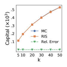
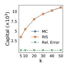
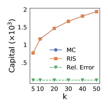
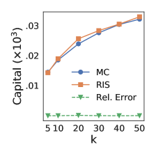
(a) Instagram	(b) FriendFeed	(c) GooglePlus	(d) Reddit

Figure 1: Capital estimation for seed sets obtained by ADITUM: RIS-based estimation by ADITUM vs. estimation by Monte Carlo simulations, with top-25% target selection.

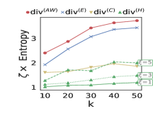
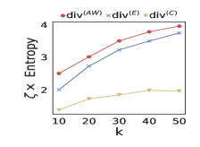
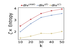
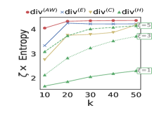
(c) Instagram	(d) FriendFeed	(a) GooglePlus	(b) Reddit

Figure 2: Entropy of the seed sets obtained by ADITUM for various diversity functions, with top-25% target selection and $\alpha=0$.

7.2 Effect of the diversity functions

To understand the impact of the diversity notion on the ADITUM performance, we inspected the degree of diversification induced by each of the functions described in Sect. 4. In particular, we first measured the cross-entropy of the distribution of attribute-values associated to the profile set of seeds, i.e.,

$$Entropy(S)=\!\!\!\!\sum_{a\in dom(S)}\frac{n_{a}}{\sum_{a^{\prime}\in dom(S)}n_{a^{\prime}}}\log\bigg{(}\frac{n_{a}}{\sum_{a^{\prime}\in dom(S)}n_{a^{\prime}}}\bigg{)}.$$

Then, we multiplied the value of $Entropy(S)$ by a factor $\zeta=(1+\log(|dom|/$ $|dom(S)|))^{-1}$ that penalizes more for smaller fraction of attribute-values covered by the profile set of $S$.

Results shown in Fig. 2 indicate that $div^{(AW)}$ generally yields seed sets with higher cross-entropy than the other diversity functions — in fact, to maximize $div^{(AW)}$, ADITUM tends to favor a uniform distribution of the attribute-values over the seed set. Also, $div^{(AW)}$ achieves higher coverage of the attribute domains (i.e., lower penalization factor). The second best diversity function is the entropy-based one, $div^{(E)}$, which shows trends similar to $div^{(AW)}$.

Conversely, $div^{(C)}$ and $div^{(H)}$ lead to less diversified seed sets. This is actually not surprising since the class-based notion of diversity relies on the grouping of the profiles (i.e., coarser grain than at attribute-value level) and it is maximized when all profiles in $S$ are chosen from different classes (i.e., $k\equiv h$, cf. Sect. 4.5), regardless of the distribution of their constituent attribute-values. In this regard, we further investigated how the combination of the budget $k$ and the number of classes (into which the profile set is partitioned) affects the diversity value. Fig. 3 shows that $div^{(C)}$ increases more rapidly with the increase in the number of classes w.r.t. $k$.

Also, the Hamming-based diversity, $div^{(H)}$, consistently behaves worse than $div^{(AW)}$ and $div^{(E)}$, while it is comparable to $div^{(C)}$ for higher radius. Indeed, $div^{(H)}$ strongly depends on the setting of the radius: as expected, the diversity increases for higher values of the radius $\xi$. This is explained since Eq. (4) increases as the union of the Hamming balls of the nodes in the seed set grows; however, setting $\xi=1$ leads to Hamming balls containing nodes that are not really different from each other. As a consequence, Eq. (4) would to be deceived because a huge Hamming ball may corresponds to a poorly diversified seed set.

In the rest of the result presentation, we will refer to the attribute-wise diversity only. Our justification is that $div^{(AW)}$ (i) has shown effectiveness in the diversification of the seed set that is as good as or better than $div^{(E)}$, while outperforming $div^{(C)}$ and $div^{(H)}$, (ii) it allows marginal gain computation that is clearly more efficient than the conditional entropy computation required in $div^{(E)}$, and (iii) it does not depend from additional a-priori knowledge like $div^{(C)}$ does, or parameters like $div^{(H)}$ does.

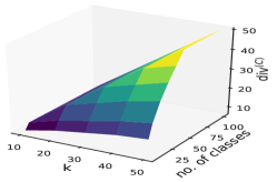
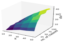
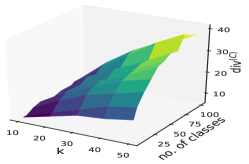
(a) $\alpha=0.0$	(b) $\alpha=0.5$	(c) $\alpha=1.0$

Figure 3: Class-based diversity on Instagram by varying the number of classes, $k$, and $\alpha$, with top-25% target selection.

7.3 Evaluation of identified seed sets

Here we discuss how the different settings of parameters in ADITUM, particularly $\alpha$ and the attribute distributions, affect the seed identification.

Sensitivity to $\alpha$.  Heatmaps in Fig. 4 show the pairwise overlaps of seed sets, normalized by $k$, for varying $\alpha$. Focusing first on the overlaps between the seed set corresponding to $\alpha=1$ (i.e., capital contribution only) and the ones corresponding to diversity at different degrees ($\alpha<1$), the overlap decreases rapidly for lower $\alpha$. (This trend is less evident for Instagram because of its tighter connectivity than FriendFeed, GooglePlus and Reddit, as in fact it corresponds to the maximal strongly connected component of the original network graph 8326536 ). While in general overlaps always change for pairs of seed sets corresponding to different settings of $\alpha$, it appears that the fading of overlaps becomes more gradual on networks with stronger small-world characteristics (i.e., GooglePlus). Moreover, results (shown in Appendix, Fig. 10) obtained at top-5% and top-10% target selection, also confirm the variability in the seed set overlap, which is again more evident on the larger networks.

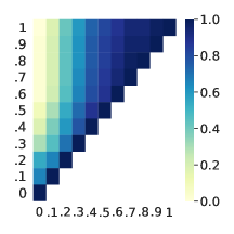
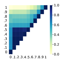
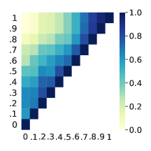
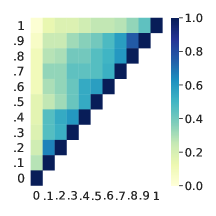
(a) Instagram	(b) FriendFeed	(c) GooglePlus	(d) Reddit

Figure 4: Normalized overlap of seed sets, for $\alpha\in[0,1]$ (with increments of $0.1$), $k=50$, top-25% target selection, and exponential distribution of attributes (except Reddit).

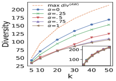
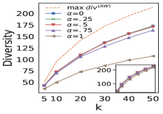
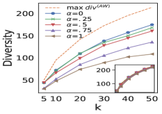
(a) Instagram	(b) FriendFeed	(c) GooglePlus

Figure 5: Exponential (main) vs. uniform (inset) distribution: attribute-wise of seed set for varying $k$ and $\alpha$, top-25% target selection, and comparison to maximum diversity value.

Effect of the attribute distribution.  The previous analysis refers to exponential distribution of the attributes. We observed however that the sensitivity of ADITUM to the setting of $\alpha$ becomes much lower when a uniform distribution law is adopted. This prompted us to investigate the reasons underlying this behavior. To this end, we compared the diversity value associated to each seed set, by varying $\alpha$ and distributions, with the maximum possible value $div^{*}[k]$ (Eq. 12); this is achieved when all the attribute values are equally distributed over the seeds.

Not surprisingly, looking at the insets of Fig. 5 that correspond to uniform distribution, we observe that the trends of seed-set diversity at varying $\alpha$ are all close to each other as well as to the maximum value. By contrast, using exponential distributions (main plots of Fig. 5), it is evident that the slope of the diversity tends to decrease with higher $\alpha$, thus increasing the gap with the maximum diversity curve. Moreover, different settings of the target selection threshold have no significant impact on the trends already observed for top-25% (results shown in Appendix, Fig. 11). In the following, results correspond to exponential distribution of the attributes, unless otherwise specified.

7.4 Comparison with DTIM

Stage 1:  We first evaluated the integration of the topology-driven diversity function 8326536 into our RIS-based framework. We analyzed the normalized overlap of seed sets obtained by ADITUM and by the resulting DTIM-based variant. Figure 6 shows low-mid lack of normalized overlap between compared seed sets; in particular, overlap is much closer to zero for the largest networks, which are also sparser (and hence, more realistic) than Instagram network.

Stage 2:  In the second stage of evaluation, we compared ADITUM and DTIM in terms of the expected capital. In Fig. 7, the insets show results of a Monte Carlo simulation (with 10 000 runs) for the estimation of the capital associated with the seed sets provided by each of the methods with $\alpha=1$ (i.e., without the diversity contribution). Also, we set $\eta=10^{-4}$ for DTIM, which means minimal path-pruning, and hence highest estimation accuracy for the competitor. We observe that ADITUM keeps a relatively small advantage over DTIM as for the estimated capital. Nonetheless, it should be emphasized that, as expected from a comparison between a RIS-based method and a greedy method, ADITUM outperforms DTIM in terms of running time, up to 3 orders of magnitude (e.g., in FriendFeed with $k\geq 10$), and this gap becomes even more evident as both $k$ and the network size increase. Note that, while the running time of DTIM tends to increase linearly in $k$, for ADITUM it may even decrease with $k$: likewise TIM+, this is a result of the interplay of the main factors that determine the number of random RR-Sets.

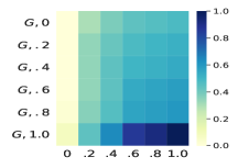
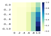
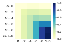
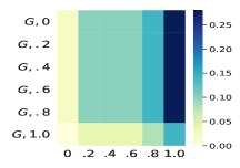
(a) Instagram	(b) FriendFeed	(c) GooglePlus	(d) Reddit

Figure 6: Topology-based vs. attribute-based diversity: Normalized overlap of seed sets, for selected values of $\alpha$, $k=50$, and top-25% target selection.

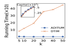
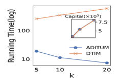
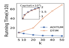
(a) Instagram	(b) FriendFeed	(c) GooglePlus

Figure 7: ADITUM ($\epsilon=0.1$) vs. DTIM ($\eta=10^{-4}$): Running time in seconds (main plot) and expected capital (inset) for varying $k$, top-25% target selection and $\alpha=1$.

7.5 Comparison with Deg-D diversity and attribute representation

As concerns the comparison with Deg-D, we again devised two stages of evaluation: (1) comparison of seed sets produced by ADITUM and by Deg-DU/Deg-DW, and (2) adaptation of our RIS framework to numerical-attribute diversity used by Deg-D (cf. Sect. 6-Setting).

Stage 1:  Fig. 9 shows the normalized overlaps of seed sets. Two main remarks can be drawn: first, the overlaps between ADITUM and Deg-D are always quite low ($0.28\sim 0.43$), and second, the setting of $\gamma$ (i.e., $1-\alpha$) has little effect on Deg-D.

Stage 2:  Fig. 9 refers to numerical attribute representation and integration of Deg-DU and Deg-DW functions into our framework, denoted as RIS-U and RIS-W. We set $\gamma=\alpha=0.5$ to equally balance the contributions of diversity and spread in the methods’ objective function. We observe that the seed-set diversity values are the same for the two methods in the uniform setting of the numerical-attribute diversity (i.e., Deg-DU and RIS-U). Conversely, in the weighted setting, the RIS-based diversity curve is only slightly below the Deg-DW curve. Also, the insets show very similar expected spread (on average over 10 000 Monte Carlo runs). Overall, this indicates flexibility of our RIS-based framework, which can also be properly adapted to integrate numerical-based diversity functions.

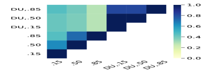
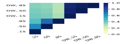
Figure 8: ADITUM vs. Deg-DU (left) and Deg-DW (right): Normalized overlap of seed sets, for $\gamma\in\{0.15,0.5,0.85\}$, $k=50$, and top-100% target selection, on MovieLens.

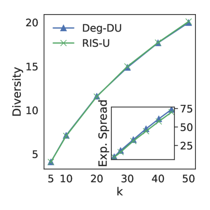
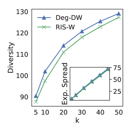
Figure 9: Deg-DU vs. RIS-U (left) and Deg-DW vs. RIS-W (right): Expected spread (inset) and seed set diversity by varying $k$, for $\gamma=0.5$, on MovieLens.

8 Conclusions

We proposed a novel targeted influence maximization problem which accounts for the diversification of the seeds according to side-information available at node level in the general form of categorical attribute values. We also design a class of nondecreasing monotone and submodular functions to determine diversity of the categorical profiles associated to seed nodes. Our developed RIS-based ADITUM algorithm was compared to two IM methods, the one exploiting topology-driven diversity and the other one accounting for numerical-based diversity in IM. While showing different and more flexible behavior than the competitors, ADITUM takes the advantages of ensuring the RIS-typical theoretical-guarantee and computational complexity under a general, side-information-based setting of node diversity. A further strength point of our diversity-sensitive framework lays on its versatility since ADITUM can easily be extended to incorporate other definitions of node diversity. In this regard, we plan to define diversity notions based on representation learning techniques, including network embedding methods.

Appendix

A Proofs of theoretical results in Section 4

Proposition 1

The attribute-wise diversity function defined in Eq. (3) is monotone and submodular.

Proof.  Function $div(S)$ in Eq. (3) is monotone and submodular provided that $div_{A}(S)$ in Eq. (4) is such as well, for any choice of $A\in\mbox{$\mathcal{A}$}$ and setting of coefficients $\omega$, since $div(S)$ is a linear combination of functions $div_{A}(S)$ with nonnegative weights. Monotonicity of Eq. (4) is trivially satisfied. As concerns submodularity, let us assume $\lambda=1$ without loss of generality. Note that the inclusion of a node $u$ into $S$ corresponds to $1/k_{1}$, with $k_{1}$ equal to the size of $S^{\prime}\subseteq S$ such that, for each $v\in S^{\prime}$, it holds that $val_{A}(v)\equiv val_{A}(u)$; moreover, the inclusion of node $u$ into $T$ ($S\subseteq T$) is $1/k_{2}$, with $k_{2}$ equal to the size of $T^{\prime}\subseteq T$ such that for each $v\in T^{\prime}$, $val_{A}(v)\equiv val_{A}(u)$. Since $S\subseteq T$, it holds that $k_{2}\geq k_{1}$, or $1/k_{1}\geq 1/k_{2}$, which concludes the proof.  $\blacksquare$

Lemma 1

Given a set $S$ and a categorical attribute $A$,  consider $M_{A}=\max_{a\in dom_{A}(S)}n_{a}$ and $m_{A}=\min_{a\in dom_{A}(S)}n_{a}$. For any

$$S=\operatornamewithlimits{argmax}_{S^{\prime}\subseteq\mathcal{V}\ s.t.\ |S^{\prime}|\leq k}div_{A}(S^{\prime}),$$

it holds that $M_{A}-m_{A}<=1.$

Proof.  Assume by contradiction that there exists a set $S$ that maximizes $div_{A}$ (for any $A\in\mbox{$\mathcal{A}$}$) such that $M_{A}-m_{A}>1$. Without loss of generality, assume $M_{A}=m_{A}+2$ and $\lambda=1$. Let $a^{(M)}$ and $a^{(m)}$ denote the categorical values corresponding to $M_{A}$ and $m_{A}$, respectively. It is easy to note that, if we remove a node with profile containing $a^{(M)}$, resp. we add a node with profile containing $a^{(m)}$, then $div_{A}$ will decrease by a quantity $\delta^{-}=1/(M_{A})$, resp. increase by a quantity $\delta^{+}=1/(m_{A}+1)$. Since $\delta^{-}<\delta^{+}$, the diversity value is increased, therefore $S$ cannot be the optimal solution, which proves our statement.  $\blacksquare$

Proposition 2

Given the set of categorical attributes $\mathcal{A}=\{A_{1},\ldots,A_{m}\}$, $m$-real valued coefficients $\omega_{j}\in[0,1]$ ($j=[1..m]$), and a budget $k$, the theoretical maximum value for Eq. (3) is function of $k$ and determined as ($d_{j}\triangleq|dom_{A_{j}}|$):

$$div^{*}[k]=\sum_{j=1}^{m}\omega_{j}\left(d_{j}\sum_{i=1}^{k/d_{j}}\frac{1}{i^{\lambda}}+\frac{k~{}\mathrm{mod}~{}d_{j}}{\big{(}1+\frac{k}{d_{j}}\big{)}^{\lambda}}\right)$$ (12)

Proof sketch.  Equation (12) can be derived based on the observation that the maximum possible value achievable w.r.t. a budget $k$ is obtained when the categorical values are equally distributed among the $k$ nodes. Without loss of generality, let us consider the case with one categorical attribute $A$. If we need to select $k$ nodes, one at a time, the best choice corresponds to select the node with value $a^{*}=\operatornamewithlimits{argmin}_{a\in dom_{A}(S)}$ $n_{a}$, as it yields the maximum marginal gain. It straightforwardly follows that, by adopting this strategy, a set $S$ can be produced to satisfy the requirement stated in Lemma 1 for the maximization of Eq. (3).  $\blacksquare$

Proposition 3

The Hamming-based diversity function defined in Eq. (8) is monotone and submodular.

Proof sketch.  Monotonicity of Eq. (8) is trivial. In fact, since the equation takes into account the union of the Hamming balls associated with any node in the set, greater sets can only lead to greater Hamming balls, thus Eq. (8) is only allowed to increase.

As concerns the submodularity, it should be noted that for any $S\subseteq T\subseteq V$, it holds that $B^{\xi}_{S}\subseteq B_{T}^{\xi}$. In light of Fact 2, we can write the inequality between the marginal gain of any node $v$ with respect to $S$ and $T$ as:

$$\begin{array}[]{lcl}\cancel{div(S)}+\mid B_{v}^{\xi}\setminus B_{S}^{\xi}\mid-\cancel{div(S)}&\geq&\cancel{div(T)}+\mid B_{v}^{\xi}\setminus B_{T}^{\xi}\mid-\cancel{div(T)}\\ \end{array}$$

In order to prove the submodularity, we can proceed by contradiction. Suppose there exists a node $v$ such that the following inequality is strictly satisfied:

$$\begin{array}[]{lcl}\cancel{\mid B_{v}^{\xi}\mid}-\mid B_{v}^{\xi}\cap B_{S}^{\xi}\mid&<&\cancel{\mid B_{v}^{\xi}\mid}-\mid B_{v}^{\xi}\cap B_{T}^{\xi}\mid\\ \mid B_{v}^{\xi}\cap B_{S}^{\xi}\mid&>&\mid B_{v}^{\xi}\cap B_{T}^{\xi}\mid\end{array}$$

It is easy to verify that the above inequality is a contradiction, in fact since $B_{S}^{\xi}\subseteq B_{T}^{\xi}$, there cannot exist any node $u$ belonging to the intersection in the leftmost side of the equation that does not belong to the intersection in the rightmost side.  $\blacksquare$

Proposition 4

The entropy-based diversity function defined in Eq. (9) is monotone and submodular.

Proof sketch.  Monotonicity and submodularity are ensured given the strict relation between the joint entropy function and a polymatroid Fujishige78 . Moreover, as concerns submodularity in particular, note that in the inequality $H(\mathcal{X}_{S},X)-H(\mathcal{X}_{S})\geq H(\mathcal{X}_{T},X)-H(\mathcal{X}_{T})$ (with $\mathcal{X}_{S}\subset\mathcal{X}_{T}\subseteq\mathcal{X}$ and $X\in\mathcal{X},X\notin\mathcal{X}_{T}$), each of the two terms is just the conditional entropy of variable $X$ given $\mathcal{X}_{S}$ and $\mathcal{X}_{T}$, respectively. Therefore, $H(X|\mathcal{X}_{S})\geq H(X|\mathcal{X}_{T})$ holds since conditioning cannot increase entropy.  $\blacksquare$

Proposition 5

Given a budget $k$ and $h$ classes, the function in Eq. (10), equipped with $\mathrm{f}(x)=\log(1+x)$, with $r_{j}=1,\forall v_{j}\in\mbox{$\mathcal{V}$}$, achieves the minimum value of $\log(1+k)$ when all $k$ nodes belong to the same class (i.e., 1 class covered), and the maximum value of $k$ when all $k$ nodes belong to different classes (i.e., $k$ classes covered).

Proof sketch.  The values of $\log(1+k)$ and $k$ are immediately derived by evaluating Eq. (10) for the cases $h=1$ and $h=k$, respectively. The proof of $k$ as upper bound is immediate. To prove that $\log(1+k)$ is the lower bound of Eq. (10), consider without loss of generality a uniform class distribution, i.e., there are $k/h$ (with $h<k$) nodes that belong to each class. In this case, it holds that $div(S)=h\log(1+k/h)$, for any size-$k$ $S$. It follows that the inequality $\log(1+k)\leq h\log(1+k/h)$ must be verified (with equality iff $h=1$). This is immediately derived by observing that, after algebraic manipulation, the above inequality holds iff $(1+k)h^{h}\leq(h+k)^{h}$, which is true since the terms on the left side are contained in the polynomial $(h+k)^{h}$.  $\blacksquare$

Proposition 6

The partition-based diversity function defined in Eq. (10) is monotone and submodular.

Proof sketch.  Monotonicity and submodularity of the function in Eq. (10) can directly be derived from the mixture property of submodular functions and the composition property of submodular with nondecreasing concave functions Lovasz83 , respectively. In fact, the summation argument of $\mathrm{f}$ is a collection of modular functions with nonnegative weights (and hence is monotone), the application of $\mathrm{f}$ yields a submodular function, and finally summing up over the groups retains monotonicity and submodularity.  $\blacksquare$

B Inappropriate set-diversity functions

We report details about a number of functions that, despite their simplicity, were demonstrated to be unsuitable as diversity functions for our problem (cf. Sect. 4.1).

Concerning attribute-wise functions, we discussed that a simple approach would be to aggregate pairwise distances of the node profiles w.r.t. a given attribute $A$. We consider in particular the following definition based on pairwise attribute-value mismatchings:

$$f_{1}(S,A)=\frac{1}{|S|}\sum_{u,v\in S}\mathbbm{1}[val_{A}(u)\neq val_{A}(v)],$$

where $\mathbbm{1}[\cdot]$ denotes the indicator function. It is easy to prove that this function is non-submodular; to give empirical evidence of this fact, consider the following example. We are given $S=\{u,v,x\}$ with $val_{A}(u)=val_{A}(v)=a_{1}$ and $val_{A}(x)=a_{2}$, and $T=\{u,v,x,y\}$ with $val_{A}(y)=a_{1}$. Suppose that node $z$, with $val_{A}(z)=a_{2}$, is inserted into $S$ and $T$, then it holds that: $f_{1}(S,A)=\frac{2}{3}$, $f_{1}(S\cup\{z\},A)=\frac{4}{4}$, $f_{1}(T,A)=\frac{3}{4}$, and $f_{1}(T\cup\{z\},A)=\frac{6}{5}$. It follows that $f_{1}(S\cup\{z\},A)-f_{1}(S,A)\not\geq f_{1}(T\cup\{z\},A)-f_{1}(T,A)$. Note also that the property of submodularity still does not hold if the normalization term (i.e., $|S|$) is discarded in $f_{1}(\cdot)$.

Let us now extend to computing pairwise distances of the node profiles in their entirety, focusing on the Hamming distance, as defined in Eq. (6). Upon this, let us define $f_{2}(S)=\sum_{u,v\in S,u\neq v}dist^{H}(u,v)$, and two normalized versions: $\widehat{f_{2}}(S)=(1/(2|S|))f_{2}(S)$ and $\widehat{\widehat{f_{2}}}(S)=(1/|S|(|S|-1))f_{2}(S)$. It is easy to check that none of such functions is appropriate. Let us consider the following example. We are given a schema with three attributes ($m=3$) and sets $S=\{u,v\}$, such that $\mbox{$\mathcal{A}$}[u]=\langle a_{1},\bot,\bot\rangle$, $\mbox{$\mathcal{A}$}[v]=\langle a_{2},\bot,\bot\rangle$, and $T=\{u,v,x\}$, such that $\mbox{$\mathcal{A}$}[x]=\langle a_{3},b_{1},c_{1}\rangle$. Suppose that node $z$, with $\mbox{$\mathcal{A}$}[z]=\langle a_{4},\bot,\bot\rangle$, is inserted into $S$ and $T$, then it holds that: $f_{2}(S)=2$, $f_{2}(T)=14$, $f_{1}(S\cup\{z\})=6$, and $f_{1}(T\cup\{z\})=24$. It follows that $f_{2}(S\cup\{z\})-f_{2}(S)\not\geq f_{2}(T\cup\{z\})-f_{2}(T)$. Considering $\widehat{f_{2}}(\cdot)$, we have: $\widehat{f_{2}}(S)=\frac{1}{2}$, $\widehat{f_{2}}(T)=\frac{7}{3}$, $\widehat{f_{2}}(S\cup\{z\})=1$, and $\widehat{f_{2}}(T\cup\{z\})=3$; thus, again $\widehat{f_{2}}(S\cup\{z\})-\widehat{f_{2}}(S)\not\geq\widehat{f_{2}}(T\cup\{z\})-\widehat{f_{2}}(T)$. Yet, when using $\widehat{\widehat{f_{2}}}(\cdot)$, we have: $\widehat{\widehat{f_{2}}}(S)=1$, $\widehat{\widehat{f_{2}}}(T)=\frac{7}{3}$, $\widehat{\widehat{f_{2}}}(S\cup\{z\})=1$, and $\widehat{\widehat{f_{2}}}(T\cup\{z\})=2$; in this case, mononicity is not even satisfied (since $\widehat{\widehat{f_{2}}}(T\cup\{z\})\not\geq\widehat{\widehat{f_{2}}}(T)$).

Alternatively, we considered Jaccard distance, i.e., given the profiles of any two nodes $u,v$:

$$dist^{J}(u,v)=1-\frac{\sum_{j=1}^{m}\mathbbm{1}[val_{A_{j}}(u)=val_{A_{j}}(v)]}{|\mbox{$\mathcal{A}$}[u]|+|\mbox{$\mathcal{A}$}[v]|-\sum_{j=1}^{m}\mathbbm{1}[val_{A_{j}}(u)=val_{A_{j}}(v)]}.$$

Upon this, let us define $f_{3}(S)=\sum_{u,v\in S,u\neq v}dist^{J}(u,v)$, and normalized version: $\widehat{f_{3}}(S)=(1/(2|S|))f_{2}(S)$. Like previous functions, it can be empirically shown that $f_{3}(\cdot)$ and $\widehat{f_{3}}(\cdot)$ are not appropriate for our purposes. Suppose we are given a schema with five attributes ($m=5$) and sets $S=\{u,v\}$, such that $\mbox{$\mathcal{A}$}[u]=\langle a,b,c,\bot,\bot\rangle$, $\mbox{$\mathcal{A}$}[v]=\langle a,b,\bot,d,\bot\rangle$, and $T=\{u,v,x\}$, such that $\mbox{$\mathcal{A}$}[x]=\mbox{$\mathcal{A}$}[v]$. Suppose that node $z$, with $\mbox{$\mathcal{A}$}[z]=\langle a,\bot,\bot,d,e\rangle$, is inserted into $S$ and $T$, then it holds that: $f_{3}(S)=1,f_{3}(T)=2,f_{3}(S\cup\{z\})=\frac{18}{5},f_{3}(T\cup\{z\})=\frac{28}{5}$. It follows that $f_{3}(S\cup\{z\})-f_{3}(S)\not\geq f_{3}(T\cup\{z\})-f_{3}(T)$. Considering $\widehat{f_{3}}(\cdot)$, we have: $\widehat{f_{3}}(S)=\frac{1}{4}$, $\widehat{f_{2}}(T)=\frac{1}{3}$, $\widehat{f_{2}}(S\cup\{z\})=\frac{3}{5}$, and $\widehat{f_{2}}(T\cup\{z\})=\frac{7}{10}$; thus, again $\widehat{f_{3}}(S\cup\{z\})-\widehat{f_{3}}(S)\not\geq\widehat{f_{3}}(T\cup\{z\})-\widehat{f_{3}}(T)$.

The above Jaccard distance function could also be exploited to allow for measuring the dissimilarity of all profiles in any set $S=\{v_{1},\ldots,v_{k}\}\subseteq\mbox{$\mathcal{V}$}$:

$$f_{4}(S)=1-\frac{\sum_{j=1}^{m}\mathbbm{1}[val_{A_{j}}(v_{1})=\ldots=val_{A_{j}}(v_{k})]}{\sum_{j=1}^{m}|\bigcup_{v\in S}\{val_{A_{j}}(v)\}|}.$$

However, it is straightforward to show that the above function can easily yield useless results; e.g., referring to the previous example, the marginal gains of $z$ w.r.t. $S$ and $T$ are the same. Even worse, a normalization of $f_{4}(S)$ by set-size does not even ensure monotonicity.

C Complexity aspects of ADITUM

Proposition 7

ADITUM runs in $O((k+l)(|\mbox{$\mathcal{E}$}|+|\mbox{$\mathcal{V}$}|)$ $\log|\mbox{$\mathcal{V}$}|/\epsilon^{2})$ time and returns a $(1-1/e-\epsilon)$-approximate solution with at least $1-|\mbox{$\mathcal{V}$}|^{-l}$ probability.

Proof sketch.  ADITUM is developed under the RIS framework and follows the typical two-phase schema of TIM/ TIM+ methods, i.e., parameter estimation and (seed) node selection, for which the theoretical results in the Proposition hold. Due to the targeted nature of the problem under consideration, the expected capital must be computed in place of the expected spread; however, this only implies to choose a distribution over the roots of the RR-Sets, which depends on the target scores of the nodes in the network. Thus, the asymptotic complexity of TIM/TIM+ is not increased. Moreover, two major differences occur in the seeds selection phase of ADITUM w.r.t. TIM/TIM+, i.e., the lazy forward approach and the computation of the marginal gain w.r.t. the diversity function. However, both aspects do not affect the asymptotic complexity, since the former allows saving runtime only and the latter does not represent any overhead (computing a node’s marginal gain is made in nearly constant time, for each of the diversity functions). Therefore, we can conclude that ADITUM has the same asymptotic complexity of TIM/TIM+.  $\blacksquare$

D Sensitivity to $\alpha$

Figure 10 shows further results on normalized overlap of seed sets, for top-5% and top-10% target selection threshold.

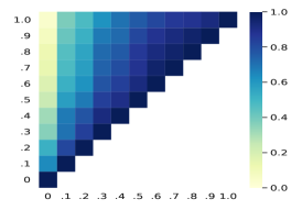
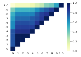
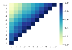
(a) Instagram	(b) FriendFeed	(c) GooglePlus
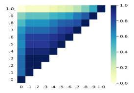
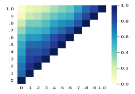
(d) Instagram	(e) FriendFeed	(f) GooglePlus

Figure 10: Normalized overlap of seed sets, for $\alpha\in[0,1]$ (with increments of $0.1$), $k=50$, top-5% (top) and top-10% (bottom) target selection, and exponential distribution of attributes.

E Effect of the attribute distribution

Figure 11 shows further results on comparison between exponential and uniform distributions, for top-5% and top-10% target selection threshold.

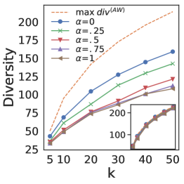
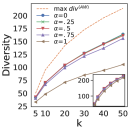
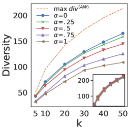
(a) Instagram	(b) FriendFeed	(c) GooglePlus
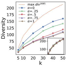
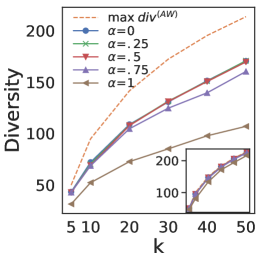
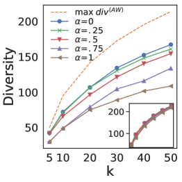
(d) Instagram	(e) FriendFeed	(f) GooglePlus

Figure 11: Exponential (main) vs. uniform (inset) distribution: seed-set diversity for varying $k$ and $\alpha$, top-5% (a–c) and top-10% (d–f) target selection, and comparison to maximum diversity value.

References

- (1) Banerjee, S., Jenamani, M., Pratihar, D.K.: ComBIM: A community-based solution approach for the Budgeted Influence Maximization Problem. Expert Systems with Applications 125, 1–13 (2019)
- (2) Bao, Q., Cheung, W.K., Zhang, Y.: Incorporating structural diversity of neighbors in a diffusion model for social networks. In: Proc. IEEE/WIC/ACM Int. Conf. on Web Intelligence, pp. 431–438 (2013)
- (3) Borgs, C., Brautbar, M., Chayes, J., Lucier, B.: Maximizing social influence in nearly optimal time. In: Proc. ACM-SIAM Symp. on Discrete Algorithms (SODA), pp. 946–957 (2014)
- (4) Caliò, A., Interdonato, R., Pulice, C., Tagarelli, A.: Topology-driven Diversity for Targeted Influence Maximization with Application to User Engagement in Social Networks. IEEE Trans. Knowl. Data Eng. 30(12), 2421–2434 (2018)
- (5) Chen, W., Lakshmanan, L.V.S., Castillo, C.: Information and Influence Propagation in Social Networks. Morgan & Claypool (2013)
- (6) Cover, T.M., Thomas, J.A.: Elements of Information Theory. John Wiley & Sons, Inc. (2006)
- (7) Deng, X., Pan, Y., Shen, H., Gui, J.: Credit distribution for influence maximization in online social networks with node features. J Intell Fuzzy Syst 31(2), 979–990 (2016)
- (8) Fujishige, S.: Polymatroid dependence structure of a set of random variables. Inform. Contr. 39, 55–72 (1978)
- (9) Goyal, A., Lu, W., Lakshmanan, L.V.S.: Simpath: An efficient algorithm for influence maximization under the linear threshold model. In: 2011 IEEE 11th International Conference on Data Mining, pp. 211–220 (2011)
- (10) Guler, B., Varan, B., Tutuncuoglu, K., Nafea, M.S., Zewail, A.A., Yener, A., Octeau, D.: Optimal strategies for targeted influence in signed networks. In: Proc. Int. Conf. on Advances in Social Networks Analysis and Mining (ASONAM), pp. 906–911 (2014)
- (11) Guo, J., Zhang, P., Zhou, C., Cao, Y., Guo, L.: Personalized influence maximization on social networks. In: Proc. ACM Conf. on Information and Knowledge Management (CIKM), pp. 199–208 (2013)
- (12) Huang, P., Liu, H., Chen, C., Cheng, P.: The impact of social diversity and dynamic influence propagation for identifying influencers in social networks. In: Proc. IEEE/WIC/ACM Int. Conf. on Web Intelligence, pp. 410–416 (2013)
- (13) Interdonato, R., Pulice, C., Tagarelli, A.: "got to have faith!": The devotion algorithm for delurking in social networks. In: 2015 IEEE/ACM International Conference on Advances in Social Networks Analysis and Mining (ASONAM), pp. 314–319 (2015)
- (14) Kempe, D., Kleinberg, J.M., Tardos, É.: Maximizing the spread of influence through a social network. In: Proc. ACM SIGKDD Int. Conf. on Knowledge Discovery and Data Mining (KDD), pp. 137–146 (2003)
- (15) Kumar, S., Hamilton, W.L., Leskovec, J., Jurafsky, D.: Community interaction and conflict on the web. In: Proceedings of the 2018 World Wide Web Conference on World Wide Web, pp. 933–943 (2018)
- (16) Lagnier, C., Denoyer, L., Gaussier, E., Gallinari, P.: Predicting information diffusion in social networks using content and user’s profiles. In: Proc. European Conf. on Information Retrieval (ECIR), pp. 74–85 (2013)
- (17) Lee, J., Chung, C.: A query approach for influence maximization on specific users in social networks. IEEE Trans Knowl Data Eng 27(2), 340–353 (2015)
- (18) Li, H., Bhowmick, S., Sun, A., Cui, J.: Conformity-aware influence maximization in online social networks. The VLDB Journal 24, 117–141 (2015)
- (19) Li, X., Smith, J.D., Dinh, T.N., Thai, M.T.: Why approximate when you can get the exact? Optimal targeted viral marketing at scale. In: Proc. IEEE Conf. on Computer Communications (INFOCOM), pp. 1–9 (2017)
- (20) Li, Y., Fan, J., Wang, Y., Tan, K.: Influence maximization on social graphs: A survey. IEEE Transactions on Knowledge and Data Engineering 30(10), 1852–1872 (2018)
- (21) Li, Y., Zhang, D., Tan, K.L.: Real-time targeted influence maximization for online advertisements. Proc. VLDB Endow. 8(10), 1070–1081 (2015)
- (22) Lovász, L.: Submodular functions and convexity. In: A. Bachem, B. Korte, M. Grötschel (eds.) Mathematical Programming: The State of the Art, pp. 235–257. Springer-Verlag Berlin Heidelberg (1983)
- (23) Lu, W., Chen, W., Lakshmanan, L.V.S.: From competition to complementarity: Comparative influence diffusion and maximization. Proc. VLDB Endow. 9(2), 60–71 (2015)
- (24) Nguyen, H.T., Dinh, T.N., Thai, M.T.: Cost-aware Targeted Viral Marketing in billion-scale networks. In: Proc. IEEE Conf. on Computer Communications (INFOCOM), pp. 1–9 (2016)
- (25) Peng, S., Zhou, Y., Cao, L., Yu, S., Niu, J., Jia, W.: Influence analysis in social networks: A survey. Journal of Network and Computer Applications 106, 17–32 (2018)
- (26) Prasad, A., Jegelka, S., Batra, D.: Submodular meets structured: Finding diverse subsets in exponentially-large structured item sets. arXiv CoRR abs/1411.1752 (2014)
- (27) Qiu, L., Jia, W., Yu, J., Fan, X., Gao, W.: PHG: A Three-Phase Algorithm for Influence Maximization Based on Community Structure. IEEE Access 7, 62511–62522 (2019)
- (28) Santos, R.L.T., Macdonald, C., Ounis, I.: Search result diversification. Found. Trends Inf. Retr. 9(1), 1–90 (2015)
- (29) Sumith, N., Annappa, B., Bhattacharya, S.: Influence maximization in large social networks: Heuristics, models and parameters. Future Generation Computer Systems 89, 777–790 (2018)
- (30) Tang, F., Liu, Q., Zhu, H., Chen, E., Zhu, F.: Diversified social influence maximization. In: Proc. IEEE/ACM Int. Conf. on Advances in Social Networks Analysis and Mining (ASONAM), pp. 455–459 (2014)
- (31) Tang, Y., Shi, Y., Xiao, X.: Influence Maximization in Near-Linear Time: A Martingale Approach. In: Proc. ACM SIGMOD Int. Conf. on Management of Data (SIGMOD), pp. 1539–1554 (2015)
- (32) Tang, Y., Xiao, X., Shi, Y.: Influence Maximization: Near-optimal Time Complexity Meets Practical Efficiency. In: Proc. ACM SIGMOD Int. Conf. on Management of Data (SIGMOD), pp. 75–86 (2014)
- (33) Wu, L., Liu, Q., Chen, E., Yuan, N.J., Guo, G., Xie, X.: Relevance meets coverage: A unified framework to generate diversified recommendations. ACM Trans. Intell. Syst. Technol. 7(3), 39:1–39:30 (2016)
- (34) Yang, D., Hung, H., Lee, W., Chen, W.: Maximizing acceptance probability for active friending in online social networks. In: Proc. ACM SIGKDD Int. Conf. on Knowledge Discovery and Data Mining (KDD), pp. 713–721 (2013)
- (35) Zhang, K., Zhang, Z., Wu, Y., Xu, J., Niu, Y.: A core theory based algorithm for influence maximization in social networks. In: 2017 IEEE International Conference on Computer and Information Technology (CIT), pp. 31–36 (2017)
- (36) Zhou, J., Zhang, Y., Cheng, J.: Preference-based mining of top- influential nodes in social networks. Future Generation Comp. Syst. 31, 40–47 (2014)