Deep Prototypical Networks Based
Domain Adaptation for Fault Diagnosis
Abstract
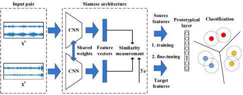
Due to the existence of dataset shifts, the distributions of data acquired from different working conditions show significant differences in real-world industrial applications, which leads to performance degradation of traditional machine learning methods. This work provides a framework that combines supervised domain adaptation with prototype learning for fault diagnosis. The main idea of domain adaptation is to apply the Siamese architecture to learn a latent space where the mapped features are inter-class separable and intra-class similar for both source and target domains. Moreover, the prototypical layer utilizes the features from Siamese architecture to learn prototype representations of each class. This supervised method is attractive because it needs very few labeled target samples. Moreover, it can be further extended to address the problem when the classes from the source and target domains are not completely overlapping. The model must generalize to unseen classes in the source dataset, given only a few examples of each new target class. Experimental results, on the Case Western Reserve University bearing dataset, show the effectiveness of the proposed framework. With increasing target samples in training, the model quickly converges with high classification accuracy.
Index Terms:
Fault diagnosis, time series classification, domain adaptation, prototype learning.I Introduction
The advances in the manufacturing industry make the volume of data proliferate. Making full use of the manufacturing big data, it can further promote industrial development. The sensor data that contain machine health information play an essential role in fault diagnosis and prognosis. In the past decades, many fault diagnosis methods have been proposed[1, 2, 3, 4, 5, 6]. Because the physics-based methods usually require specific a priori knowledge, they are laborious to implement as the industrial environment changes. Compared with traditional physics-based models, data-driven methods have attracted much attention due to their effectiveness and flexibility. Studies that combine signal processing and machine learning techniques have obtained impressive results in many industrial cases[7, 8, 9, 10, 11]. In [12], an automatic deep feature learning method uses time-frequency images to train a deep convolutional neural network for bearing fault diagnosis. Glowacz et al.[13] proposed a new feature extraction method called MSAF-20-MULTIEXPANDED. The features extracted from acoustic signals of the single-phase induction motor are classified by machine learning methods. In [14], the maximum kurtosis spectral entropy deconvolution (MKSED) method that uses the signal denoised by Ensemble Empirical Mode Decomposition (EEMD) is applied to classify bearing fault.
However, most of the intelligent fault diagnosis methods require a large amount of labeled data (target data) for training, which restricts their extensive applications. Several situations that could not obtain sufficient samples to train the deep model[15]. (1) In many applications, the process from degradation to the failure might take a long time, e.g., generators or jet engines[16]. Therefore, it is difficult to collect related data. (2) The fault detection system does not allow critical machines to operate in fault states. Once the system detects a fault, it immediately shut down the machine, which results in collecting only a few fault samples. (3) The working conditions frequently change in actual tasks, and the fault signal could be collected from different working conditions, even from different machines. It is difficult to collect sufficient samples for every type of fault. Meanwhile, the samples of similar faults usually show significant distribution discrepancies. It indicates that the model trained in one situation is not suitable for another. It is difficult or even impossible to recollect the new labeled data to train a model for the actual task. When it is difficult to collect the target data, the typical approach is to use available datasets (source data) for training the related target model. Therefore, it is vital to adapt the useful information from the source training task to a new but related diagnosis task with a few labeled target samples.
The domain adaptation, which can transfer the knowledge from the source domain to a different but related target domain, can be adopted in the situation where the source and target data have different distributions. Although domain adaptation techniques have recently been widely used in situations such as image classification, face recognition, object detection, and so forth[17], they have not yet been investigated thoroughly for time series classification, especially in fault diagnosis. In recent years, several fault diagnosis methods based on transfer learning have been proposed [18, 19, 20]. In [20], a framework with joint distribution adaptation (JDA) adapts the unlabeled target data to the conditional distribution. In [15], a few-shot learning neural network based on the Siamese network is used for bearing fault diagnosis with limited data.
In the field of fault diagnosis, the data-driven methods mainly focus on how to use fewer source data to learn more information or the transferability between different working conditions of the same machine. However, the amount of data is not a problem in the real-world industry, and we can slowly accumulate more labeled data. Meanwhile, different machines could have similar types of fault, and it is expensive and time-consuming to collect labeled data for all machines. Therefore, we pay more attention to the adaptation ability between source and target datasets, even if these datasets were collected from different machines.
In this work, we introduce a supervised approach for bearing fault diagnosis based on domain adaptation. The approach requires very few labeled target samples per class in training. Even one sample can significantly increase the model performance. Furthermore, the model trained on the source dataset can generalize to new classes that can only be seen in the target dataset, given only a few labeled samples of each new class. To improve the robustness, we adopt the prototype learning making the unseen classes easily distinguished. The modified network is based on the assumption that there exist prototypes that can represent corresponding classes in the latent space. To do this, we learn a non-linear mapping to minimize the discrepancy between source and target distributions in a latent space by neural network and take a prototype to represent the center of each class. The classification task is then simplified to find the nearest class prototype. The framework was verified on the standard Case Western Reserve University Bearing Datasets[21], which showed that our approach is effective in fault diagnosis with very few labeled target samples.
The rest of the paper is organized as follows. Section II reviews related works about domain adaptation and prototype learning. Section III describes the problem formulation and proposed framework. A series of experiments are carried out in Section IV. Finally, conclusions and future works are presented in Section V.
II Relation works
Domain adaptation. Due to the existence of dataset bias[22, 23, 24] and data shifts (e.g., prior shift, covariate shift[25], concept shift[26]) between different data sources, the model trained on one dataset is not suitable for another. Domain adaptation and transfer learning are two sub-fields of machine learning that are used to solve these problems.
Compared with the general use of transfer learning, the domain adaptation focuses on how to deal with different probability distributions of datasets. Therefore, prior methods of domain adaptation mainly try to minimize the discrepancy between the source and target samples directly. In[27], the deep transfer network uses a model with shared weights to find a domain invariant space for source and target distributions. Moreover, an adaptation layer measures their differences with the Maximum Mean Discrepancy (MMD)[28] metric. In[29], the two-stream architecture model considers that the weights in corresponding layers are related but not shared. Therefore, they added a weight regularizer to account for the distance between the source and target distributions. In[30], a model combines adversarial learning with discriminative feature learning, mapping target distribution to the source feature space. According to [31, 32], these methods can be divided into three categories. Among these categories, the one that finds a shared domain subspace is concerned with accounting for the assumption that source and target conditioned label distributions are similar, and there exists a classifier that can work well on both source and target distributions[33]. In this category, Siamese networks[34] are suitable for minimizing the discrepancy of different domains in latent space. The literature[31] uses a Siamese network to make the same class from different domain datasets as close as possible. Since the unseen target data is severely limited for the problem when the classes from the source and target domains are not completely overlapping, the architecture of the Siamese network is challenging to separate the new classes from each other. We modify the model by prototype learning, which improves model performance with a few target training samples.
Prototype learning. Through searching prototypes to represent the centers of the data distribution in each class, prototype learning is effective in improving the performance of classification. The simplest method of prototype learning is the unsupervised clustering, which searches the class centers used as the reduced prototypes independently[35, 36]. Since the unsupervised clustering does not consider the class information, the classification accuracy is usually lower compared with supervised classification methods. The learning vector quantization(LVQ)[37], proposed by Kohonen, supervised adjusts the weight vectors based on searching the optimal position of the prototypes. Although the convergence is not guaranteed, the attractive performance makes LVQ popular in many works. In the variations of LVQ, the parameter optimization approaches, which learn prototypes through optimizing the objective functions by gradient search, have excellent convergence property in learning[38, 39]. In [40], the prototypical networks search prototype representations of each class in a metric space. In [41], the model, which combines the prototype-based classifiers with deep convolutional neural networks, improves the model robustness. In our study, we minimize the discrepancy of source and target distributions by domain adaptation and learn the best representations of different classes, making the prototypes as far as possible from each other to improve the accuracy of classification. The main contributions of this work are summarized in the following.
-
1.
The framework uses convolutional neural networks as a basic model applied to time series classification. It can learn a domain invariant space with effective domain adaptation capacity through the Siamese architecture.
-
2.
The framework can be extended to solve the problem when the classes from the source and target domains are not completely overlapping. The model learned on the source dataset can generalize to new classes that can only be found in the target dataset, given only a few samples of each new class in training.
-
3.
Compared with the traditional classification methods, our model adds weight regularizations to adjust the distance of different prototypes, making the new class centers easily distinguished.
-
4.
With attractive robustness, disrupting the corresponding classes between source and target domains does not affect the classification accuracy, which is suitable for the complex working conditions in industrial applications.
III methods
III-A Notation
| Notation | Description | Notation | Description |
|---|---|---|---|
| Domain | Source, target | ||
| Data set | Label set | ||
| Single sample | Corresponding label | ||
| Source class number | Target class number | ||
| Source samples number | Target samples number | ||
| per class | per class | ||
| Class prototype | Prototype set | ||
| Data distribution | Prediction function | ||
| Feature extraction function | Classification function |
In this section, we describe the problem formulation and the proposed framework. A source dataset is a collection of pairs where each is the dimensional feature vector and is the corresponding label. A target dataset is denoted by . The denote the number of classes in datasets, denote the number of samples used in training of each class and denote the sets of respectively. The Table I describes the notations which are used in this work frequently.
We assume that the probability distributions of are different, i.e. and learn a prediction function which can work well on the target dataset. In general, is composed of two functions, . Here , the feature extraction function, is a mapping from the input space to a latent space , and is a classification function to predict the input label. The and denote the input and parameters of the model respectively. In our framework, we use a convolutional neural network as the feature extractor , and learn several prototypes on the extracted features for each class to predict the corresponding label. In order to simplify the model, we only learn one prototype for each class in this work, and the prototype is denoted as where represents the index of predicted class prototype. The is the p-dimensional vector.
III-B Architecture
We selected the one-dimensional convolutional neural networks with wide first-layer kernels [42] for the framework. The model architecture contains two parts, one is the feature extractor, and the other is the classification layer. The input of the feature extractor is a multi-dimensional time series. The convolutional layers perform some non-linearities to convert it into high-dimensional features. Therefore, the feature extractor’s output is an abstract representation of the input. Subsequently, we employed dropout [43] on the feature extractor’s output layer for regularization. Dropout randomly zeros some hidden units with a rate during training. Finally, we used the prototypical layer instead of the traditional classification layers. The prototypical layer transforms the high dimensional features into a p-dimensional vector which is used to approximate the corresponding prototype.
This framework is based on the assumption that there exists a latent space that could minimize the discrepancy of the same classes of source and target domains despite the similarity of their samples. It means that the model can work well when each class has its unique features, even if the distribution of the class in the source domain is different from the same class in the target domain. Meanwhile, we can learn prototypes to represent each class in this latent space by the neural networks. Compared with traditional classification layers, the sample features of the same class can make a certain degree of change around the prototypes, which improves the generalization performance of the model.
III-C Feature extractor
With the covariate shift assumption of domain adaptation[33], we could get the assumption that when we learn a domain invariant space for the source and target distributions. It means that the source and target domain classifiers could be the same, i.e., . Meanwhile, the parameters of CNN can be shared in a Siamese architecture, i.e., . Therefore, we can directly apply the model learned on training data to the target dataset.
In that case, the method assumes that , and we could train the function by minimizing a distance loss
| (1) |
where the denotes the mathematical expectation and the denotes the consistency of two input streams. One of the input streams comes from the source domain, and the other comes from the target domain. When the two input streams are from the same classes, , otherwise, . Therefore, we take Binary Cross-Entropy Loss as , and the function could be any metrics for similarity measurement. In this work, the function is computed with Euclidean distance, , where denotes the Sigmoid function and is a hyper-parameter that controls the distance mapping. The purpose of (1) is to minimize the discrepancy between the source and target features in the latent space.
The graphic description of our model can be found in Fig. 1. This model uses the Siamese architecture based on deep convolutional neural networks as the feature extractor. The CNN architecture is detailed in Table II. In order to avoid the interference of the high-frequency noises in industrial environments, the model uses wide kernels to extract features in the first layer and then uses small kernels to get better feature representations.
| Layer | Name | Size/Stride |
|---|---|---|
| 1 | Convolutional-ReLU | 16 filters of |
| 2 | Max-Pooling | |
| 3 | Convolutional-ReLU | 32 filters of |
| 4 | Max-Pooling | |
| 5 | Convolutional-ReLU | 64 filters of |
| 6 | Max-Pooling | |
| 7 | Convolutional-ReLU | 64 filters of |
| 8 | Max-Pooling | |
| 9 | Convolutional-ReLU | 64 filters of |
| 10 | Max-Pooling | |
| 11 | Fully-connected-Sigmoid | 100 |
III-D Classification layer
With the abstract representations extracted by the feature extractor, traditional methods usually use loss functions (for instance, Categorical Cross-Entropy for multi-class classification (2)) to minimize classification loss.
| (2) |
The and are groundtruth and the model prediction for each class in .
| Structure of the prototypical layer | ||
|---|---|---|
| Layer | Name | Parameter |
| 12 | Dropout | |
| 13 | Fully-connected | |
| Structure of the traditional layer | ||
| Layer | Name | Parameter |
| 12 | Dropout | |
| 13 | Fully-connected-Softmax | |
In this work, we combine the feature extractor with a prototypical layer to modify the model. In order to simplify the model, we only learn one prototype for each class, and the prototypical layer computes a p-dimensional vector to approximate the corresponding prototype. After the prototypical layer described in Table III, the abstract representations are converted to p-dimensional vectors. To learn the prototypes, a distance metric is used to compute the similarity between the p-dimensional vectors and the p-dimensional prototypes. Therefore, the model has two parts of trainable parameters, one for the prediction function and the other for the prototypes . The distance can be measured by the function, e.g., . Finally, we define the classification loss as
| (3) |
where the controls the classification accuracy, is the corresponding prototype of input and the () is the hyper-parameter that changes the weight of regularizations. The loss is defined as
| (4) | ||||
| (5) |
where is a hyper-parameter that can change the hardness of probability assignment[41]. By limiting the distance between vectors and the corresponding prototypes, the regularization makes the features in the same classes more compact. Meanwhile, the regularization makes the different classes separated. By combining these regularizations, we can make the model more robust and improve classification accuracy.
Therefore, we get the modified approach by learning a deep model such that
| (6) |
The prototypical network is trained with source data, and then fine-tuned based on the few samples in
| (7) |
Finally, We use minibatch stochastic gradient descent and AdaDelta[44] with hyper-parameters and to train the model and prototypes . The model is initialized by the weight initialization in [45] and trained with a minibatch size of 64 on a single GPU.
IV Experiments
| Drive-end Data | Normal | Rolling Element | Inner Race | Outer Race (6 o’clock) | Speed (rpm) | Description | Number of samples | ||||||
| Fault Diameter (inch) | 0 | 0.007 | 0.014 | 0.021 | 0.007 | 0.014 | 0.021 | 0.007 | 0.014 | 0.021 | 1730 | Dataset A | 125010 |
| Fault Labels | 0 | 1 | 2 | 3 | 4 | 5 | 6 | 7 | 8 | 9 | |||
| Fan-end Data | Normal | Rolling Element | Inner Race | Outer Race(6 o’clock) | Speed (rpm) | Description | Number of samples | ||||||
| Fault Diameter (inch) | 0 | 0.007 | 0.014 | 0.021 | 0.007 | 0.014 | 0.021 | 0.007 | 0.014 | 0.021 | 1797 | Dataset B | 125010 |
| Fault Labels | 0 | 1 | 2 | 3 | 4 | 5 | 6 | 7 | 8 | 9 | |||
| Drive-end Data | Normal | Rolling Element | Inner Race | Outer Race(6 o’clock) | Speed (rpm) | Description | Number of samples | ||||||
| Fault Diameter (inch) | 0 | 0.007 | 0.014 | 0.021 | 0.007 | 0.014 | 0.021 | 0.007 | 0.014 | 0.021 | 1730 | Dataset C | 12506 |
| Fault Labels | 0 | 1 | 2 | * | 4 | * | * | 7 | * | 9 | |||
| Fan-end Data | Normal | Rolling Element | Inner Race | Outer Race(6 o’clock) | Speed (rpm) | Description | Number of samples | ||||||
| Fault Diameter (inch) | 0 | 0.007 | 0.014 | 0.021 | 0.007 | 0.014 | 0.021 | 0.007 | 0.014 | 0.021 | 1797 | Dataset D | 12506 |
| Fault Labels | 0 | 1 | 2 | * | 4 | * | * | 7 | * | 9 | |||
| Fan-end Data | Normal | Rolling Element | Inner Race | Outer Race(6 o’clock) | Speed (rpm) | Description | Number of samples | ||||||
| Fault Diameter (inch) | 0 | 0.007 | 0.014 | 0.021 | 0.007 | 0.014 | 0.021 | 0.007 | 0.014 | 0.021 | 1797 | Dataset E | 125010 |
| Fault Labels | 0 | 9 | 6 | 3 | 2 | 5 | 7 | 8 | 4 | 1 | |||
IV-A Data description
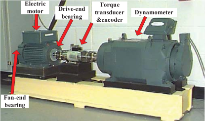
We used the Case Western Reserve University Bearing Datasets[21] to evaluate the performance of our framework. The layout of the test stand is shown in Fig. 2. Data were collected in three situations for normal bearings, single-point drive-end and fan-end defects with diameter from 0.007 to 0.028 (SKF bearings) inches. There are three types of data according to the location of defects: inner race fault, rolling element fault, and outer race fault. The outer race fault has three categories based on the fault position relative to the load zone: at 3 o’clock, at 6 o’clock, and at 12 o’clock. Each type was recorded for motor loads of 0 to 3 horsepower (speeds of 1797 to 1720 rpm) at 12kHz (some samples at 48kHz). A detailed description can be found in [46].
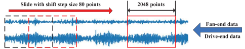
In this work, we selected 12kHz drive-end and fan-end bearing fault data to verify the adaptation ability between the datasets from different ends. As shown in Fig. 3, the samples are generated by the sliding window of 2048 size with 80 points shift step. In the experiments, we selected the fault diameters of 0.007, 0.014, and 0.021 inches for every type of fault and had ten conditions in total added with a normal condition. Datasets A, B, C, D, and E each contain 1250 samples per class, and Datasets C and D have only six classes. The details of all the datasets are described in Table IV.
In order to verify the effectiveness of the framework, we trained models by these methods: SVM, CTM (the feature extractor + traditional classification layer ()), FTM (the feature extractor ( + traditional classification layer ()) and FPM (the feature extractor () + prototypical layer ()). The SVM and CTM are trained by using the source data and n samples per class in the target dataset without domain adaptation. We randomly selected n samples per class in the target dataset for four times to generate different training sets and repeated the training for five times to calculate the mean of accuracy. In subsection E, we compared our framework with the WDMAN proposed in [47]. Our framework achieved competitive results with only one target sample per class in training.
| Task (%) | AB | BA | ||||
|---|---|---|---|---|---|---|
| n samples (per class) | 1 | 2 | 3 | 1 | 2 | 3 |
| SVM | 23.09 | 22.51 | ||||
| CTM | 48.83 | 58.32 | 67.48 | 47.84 | 64.71 | 69.74 |
| FTM | 86.28 | 98.22 | 99.46 | 95.43 | 99.80 | 99.91 |
| FPM | 92.91 | 98.52 | 99.55 | 97.53 | 99.56 | 99.72 |
IV-B Few-shot domain adaptation with complete classes in the source domain
In the first experiment, we conducted experiments on the dataset A and B to evaluate the adaptation ability of the proposed framework. We randomly selected n () samples per class in the target dataset and utilized the source dataset that contains 1250 samples per class for training. Moreover, the rest of the target data are used for testing.
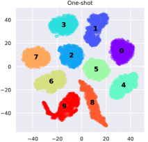
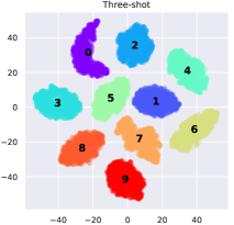
Table V reports that the classification accuracy of four methods and the number of target training samples has little effect on the performance of SVM. The proposed framework can work well even when we use only ten labeled target samples (n=1, one sample per class) for training. We also trained the base model by CTM to get the lower bound using source and a few target samples without domain adaptation. To demonstrate the adaptation ability directly, we followed the t-SNE[48] to visualize the high dimensional features in a two-dimensional map. Fig. 4 shows the visualizations of the source and target reduced features. As shown in Fig. 4, the target features learned by FPM have visible class prototypes that are close to the centers of source features, which shows that the FPM can make better use of inter-class information. Moreover, the target features are inter-class separable with only one sample per class. However, there is a problem that some samples in one class are closer to the prototypes of other classes. When using three samples per class, the target features within the same class are more compact and distinguish.
IV-C Few-shot domain adaptation with incomplete classes in the source domain
| Task (%) | CB | DA | ||||
|---|---|---|---|---|---|---|
| n samples (per class) | 1 | 3 | 5 | 1 | 3 | 5 |
| SVM | 16.68 | 30.14 | ||||
| CTM | 46.97 | 47.94 | 55.68 | 52.16 | 53.25 | 59.94 |
| FTM | 58.05 | 78.73 | 92.61 | 63.18 | 81.52 | 98.71 |
| FPM | 63.24 | 85.67 | 95.33 | 66.87 | 86.95 | 98.63 |
In real-world industrial applications, we could not obtain complete types of fault data. Therefore, we extend the model to address the problem when the classes from the source and target domains are not completely overlapping. The model must generalization to unseen classes in the source domain, given only a few examples of each new target class. In the second experiment, the model is adapted to accommodate ten classes in the target dataset when we use a few target samples and the source dataset, which contains six classes in training.
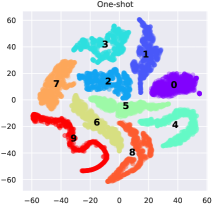
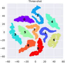
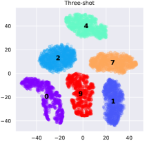
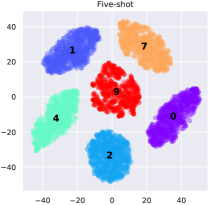
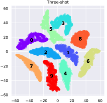
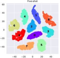
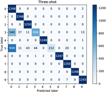
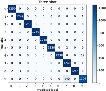
Table VI shows the classification accuracies increasing with the number of target samples available in training () rising, and FPM has improved accuracy compared with other methods. Compared with the traditional classification layer, the prototypical layer can learn the latent space where both seen and new classes are inter-class separable and intra-class compact, which proves that features learned by FPM from raw signals are more domain invariant. We visualized the features of task DA in Fig. 5, which showed that the model learned by FPM is easier to distinguish the new class features in the target domain. As shown in the Fig. 5(c), the samples in class 3 are close to the prototype of class 5 when using three target samples per class in training. To better show the effect of FPM, we calculated the confusion matrix to visualize the classification results. From Fig. 6(a), classes 3 and 5 perform poorly due to lack of training samples. The Fig. 6(b) shows that the model quickly converges with high classification accuracy as the number of target samples available in training increases.
IV-D Few-shot domain adaptation with randomized label assignments
| Task (%) | AE | EA | ||||
|---|---|---|---|---|---|---|
| n samples (per class) | 1 | 2 | 3 | 1 | 2 | 3 |
| SVM | 19.16 | 10.18 | ||||
| CTM | 43.86 | 45.27 | 62.43 | 52.98 | 57.85 | 70.22 |
| FTM | 81.71 | 97.62 | 98.82 | 92.42 | 98.73 | 99.40 |
| FPM | 92.30 | 99.12 | 99.65 | 95.86 | 99.46 | 99.73 |
In real-world industrial applications, we could not obtain any labeled target samples for some types of faults. With massive unlabeled target data, we can utilize the most different samples to represent the respective types of faults. Since we do not know the types of faults in advance, the representative target sample labels will be randomly scrambled. In order to verify the robustness of the proposed framework, we randomly disrupted the class labels of dataset B to get dataset E. In the third experiment, we followed the setting of the first experiment but replaced the dataset B with dataset E. From Table VII, there are little differences between the accuracies of the first task and third task, which proves the assumption in Section III. The performance of the framework does not rely on the similarity between the same classes in source and target domains. It extracts unique features for each class and maps the same class features to a common latent space. Therefore, the proposed framework can compensate for great domain shifts very well.
IV-E Comparison experiments
| Task (%) | WDMAN | FTM | FPM | ||
| [47] | 1 | 2 | 1 | 2 | |
| AB | 99.73 | 94.98 | 99.12 | 99.27 | 99.73 |
| AC | 99.67 | 93.13 | 97.51 | 99.40 | 99.94 |
| AD | 100 | 96.37 | 99.79 | 99.56 | 99.90 |
| BA | 99.13 | 99.26 | 99.81 | 99.53 | 99.84 |
| BC | 100 | 100 | 100 | 99.67 | 99.93 |
| BD | 99.93 | 99.99 | 100 | 99.50 | 99.91 |
| CA | 98.53 | 97.08 | 98.46 | 98.80 | 99.25 |
| CB | 99.80 | 97.48 | 99.35 | 99.12 | 99.76 |
| CD | 100 | 100 | 100 | 99.72 | 99.95 |
| DA | 98.07 | 97.09 | 98.35 | 97.91 | 98.13 |
| DB | 98.27 | 85.78 | 94.33 | 91.54 | 99.03 |
| DC | 99.53 | 95.59 | 99.12 | 99.41 | 99.78 |
We evaluated the performance of our framework on the CWRU bearing datasets and followed the experiment settings described in [47]. Unlike the experiment settings above, the adaptation ability is verified on the data from the same end. The datasets A, B, C, and D were drawn from four different motor loads (0, 1, 2, and 3 hp) with a sampling frequency of 12 kHZ. There are ten classes in total for each dataset, and their settings are the same as Table IV, which consists of nine types of fault and a normal condition. Each class contains 500 samples whose sizes are equal to 1200.
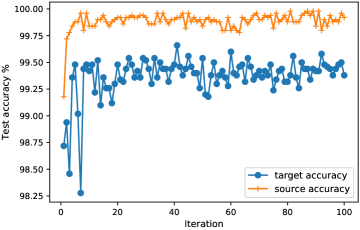
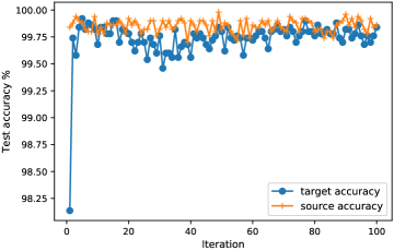
As shown in Table VIII, we compared our framework with the WDMAN proposed in [47]. With only one target sample per class in training, the FPM shows attractive results except for task DB. And we can improve the accuracy of task DB to 99.03% when using two target samples per class. Although the WDMAN does not require the labeled target samples in training, our framework requires very few labeled target samples, and the performance of the model can be improved as the labeled target samples increases. This framework is simpler than the unsupervised methods which use more than thousands of unlabeled target samples in training. Without the pre-training process, the model can be applied directly to the target dataset. Compared with the arduous training of the Generative Adversarial Networks (GAN) in WDMAN, this model can quickly converge to a high accuracy as the labeled target samples increase in training. To demonstrate the speed of convergence, we plotted the classification accuracy of task AB in Fig. 7. As shown in Fig. 7, the target domain can achieve high accuracy with few training epochs by FPM. Compared with only one target sample per class in training, the classification accuracy of the target domain is very close to that of the source domain when using two samples, which shows that the framework has an effective adaptation ability.
V Conclusion
We have introduced a deep model in combination with domain adaptation and prototype learning for fault diagnosis. This deep model takes raw temporal signals as inputs and achieves a high classification accuracy on the CWRU bearing datasets. Without changing the model architecture, the proposed framework can be applied to address the problem when the classes from the source and target domains are not completely overlapping. Our experiments show that the framework has an effective adaptation ability, which requires a few samples from a priori fixed target distribution. Moreover, the model accuracy can converge quickly as the labeled target samples increase in training. In future work, we will utilize other metrics for similarity measurement (e.g., Maximum Mean Discrepancy) instead of Euclidean distance and increase the number of prototypes for each class. In the experiments, we found that there are some differences in model performance as the randomly selected target training data changes, especially when using only one sample per class in training. For future work, we hope to further optimize the loss function to reduce the number of hyper-parameters and improve model stability. Overall, the effectiveness of the proposed framework makes it a promising method for fault diagnosis.
References
- [1] Y. Li, T. Kurfess, and S. Liang, “Stochastic prognostics for rolling element bearings,” Mechanical Systems and Signal Processing, vol. 14, no. 5, pp. 747–762, 2000.
- [2] M. Dong and D. He, “Hidden semi-markov model-based methodology for multi-sensor equipment health diagnosis and prognosis,” European Journal of Operational Research, vol. 178, no. 3, pp. 858–878, 2007.
- [3] S. Simani, C. Fantuzzi, and R. J. Patton, “Model-based fault diagnosis techniques,” in Model-based Fault Diagnosis in Dynamic Systems Using Identification Techniques. Springer, 2003, pp. 19–60.
- [4] D. Lee, V. Siu, R. Cruz, and C. Yetman, “Convolutional neural net and bearing fault analysis,” in Proceedings of the International Conference on Data Mining (DMIN). The Steering Committee of The World Congress in Computer Science, Computer …, 2016, p. 194.
- [5] P. M. Frank and B. Köppen-Seliger, “Fuzzy logic and neural network applications to fault diagnosis,” International journal of approximate reasoning, vol. 16, no. 1, pp. 67–88, 1997.
- [6] J. Liu, W. Luo, X. Yang, and L. Wu, “Robust model-based fault diagnosis for pem fuel cell air-feed system,” IEEE Transactions on Industrial Electronics, vol. 63, no. 5, pp. 3261–3270, 2016.
- [7] C. Aldrich and L. Auret, Unsupervised process monitoring and fault diagnosis with machine learning methods. Springer, 2013.
- [8] F. Lv, C. Wen, Z. Bao, and M. Liu, “Fault diagnosis based on deep learning,” in 2016 American Control Conference (ACC). IEEE, 2016, pp. 6851–6856.
- [9] R. Jegadeeshwaran and V. Sugumaran, “Fault diagnosis of automobile hydraulic brake system using statistical features and support vector machines,” Mechanical Systems and Signal Processing, vol. 52, pp. 436–446, 2015.
- [10] M. Elforjani and S. Shanbr, “Prognosis of bearing acoustic emission signals using supervised machine learning,” IEEE Transactions on industrial electronics, vol. 65, no. 7, pp. 5864–5871, 2017.
- [11] I. Martin-Diaz, D. Morinigo-Sotelo, O. Duque-Perez, and R. J. Romero-Troncoso, “An experimental comparative evaluation of machine learning techniques for motor fault diagnosis under various operating conditions,” IEEE Transactions on Industry Applications, vol. 54, no. 3, pp. 2215–2224, 2018.
- [12] D. Verstraete, A. Ferrada, E. L. Droguett, V. Meruane, and M. Modarres, “Deep learning enabled fault diagnosis using time-frequency image analysis of rolling element bearings,” Shock and Vibration, vol. 2017, 2017.
- [13] A. Glowacz, W. Glowacz, Z. Glowacz, and J. Kozik, “Early fault diagnosis of bearing and stator faults of the single-phase induction motor using acoustic signals,” Measurement, vol. 113, pp. 1–9, 2018.
- [14] Z. Wang, J. Zhou, J. Wang, W. Du, J. Wang, X. Han, and G. He, “A novel fault diagnosis method of gearbox based on maximum kurtosis spectral entropy deconvolution,” IEEE Access, vol. 7, pp. 29 520–29 532, 2019.
- [15] A. Zhang, S. Li, Y. Cui, W. Yang, R. Dong, and J. Hu, “Limited data rolling bearing fault diagnosis with few-shot learning,” IEEE Access, vol. 7, pp. 110 895–110 904, 2019.
- [16] N. Gebraeel, A. Elwany, and J. Pan, “Residual life predictions in the absence of prior degradation knowledge,” IEEE Transactions on Reliability, vol. 58, no. 1, pp. 106–117, 2009.
- [17] M. Wang and W. Deng, “Deep visual domain adaptation: A survey,” Neurocomputing, vol. 312, pp. 135–153, 2018.
- [18] W. Lu, B. Liang, Y. Cheng, D. Meng, J. Yang, and T. Zhang, “Deep model based domain adaptation for fault diagnosis,” IEEE Transactions on Industrial Electronics, vol. 64, no. 3, pp. 2296–2305, 2016.
- [19] L. Guo, Y. Lei, S. Xing, T. Yan, and N. Li, “Deep convolutional transfer learning network: A new method for intelligent fault diagnosis of machines with unlabeled data,” IEEE Transactions on Industrial Electronics, vol. 66, no. 9, pp. 7316–7325, 2018.
- [20] T. Han, C. Liu, W. Yang, and D. Jiang, “Deep transfer network with joint distribution adaptation: A new intelligent fault diagnosis framework for industry application,” ISA transactions, 2019.
- [21] “Case western reserve university bearing data center website,” http://csegroups.case.edu/bearingdatacenter/home.
- [22] J. Ponce, T. L. Berg, M. Everingham, D. A. Forsyth, M. Hebert, S. Lazebnik, M. Marszalek, C. Schmid, B. C. Russell, A. Torralba et al., “Dataset issues in object recognition,” in Toward category-level object recognition. Springer, 2006, pp. 29–48.
- [23] A. Torralba, A. A. Efros et al., “Unbiased look at dataset bias.” in CVPR, vol. 1, no. 2. Citeseer, 2011, p. 7.
- [24] T. Tommasi, N. Patricia, B. Caputo, and T. Tuytelaars, “A deeper look at dataset bias,” in Domain adaptation in computer vision applications. Springer, 2017, pp. 37–55.
- [25] H. Shimodaira, “Improving predictive inference under covariate shift by weighting the log-likelihood function,” Journal of statistical planning and inference, vol. 90, no. 2, pp. 227–244, 2000.
- [26] P. Vorburger and A. Bernstein, “Entropy-based concept shift detection,” in Sixth International Conference on Data Mining (ICDM’06). IEEE, 2006, pp. 1113–1118.
- [27] E. Tzeng, J. Hoffman, N. Zhang, K. Saenko, and T. Darrell, “Deep domain confusion: Maximizing for domain invariance,” arXiv preprint arXiv:1412.3474, 2014.
- [28] A. Gretton, K. Borgwardt, M. Rasch, B. Schölkopf, and A. J. Smola, “A kernel method for the two-sample-problem,” in Advances in neural information processing systems, 2007, pp. 513–520.
- [29] A. Rozantsev, M. Salzmann, and P. Fua, “Beyond sharing weights for deep domain adaptation,” IEEE transactions on pattern analysis and machine intelligence, vol. 41, no. 4, pp. 801–814, 2018.
- [30] E. Tzeng, J. Hoffman, K. Saenko, and T. Darrell, “Adversarial discriminative domain adaptation,” in The IEEE Conference on Computer Vision and Pattern Recognition (CVPR), July 2017.
- [31] S. Motiian, M. Piccirilli, D. A. Adjeroh, and G. Doretto, “Unified deep supervised domain adaptation and generalization,” in Proceedings of the IEEE International Conference on Computer Vision, 2017, pp. 5715–5725.
- [32] S. Motiian, Q. Jones, S. Iranmanesh, and G. Doretto, “Few-shot adversarial domain adaptation,” in Advances in Neural Information Processing Systems, 2017, pp. 6670–6680.
- [33] S. Ben-David, T. Lu, T. Luu, and D. Pál, “Impossibility theorems for domain adaptation,” in International Conference on Artificial Intelligence and Statistics, 2010, pp. 129–136.
- [34] S. Chopra, R. Hadsell, Y. LeCun et al., “Learning a similarity metric discriminatively, with application to face verification,” in CVPR (1), 2005, pp. 539–546.
- [35] J. C. Bezdek, T. R. Reichherzer, G. S. Lim, and Y. Attikiouzel, “Multiple-prototype classifier design,” IEEE Transactions on Systems, Man, and Cybernetics, Part C (Applications and Reviews), vol. 28, no. 1, pp. 67–79, 1998.
- [36] C.-L. Liu and M. Nakagawa, “Evaluation of prototype learning algorithms for nearest-neighbor classifier in application to handwritten character recognition,” Pattern Recognition, vol. 34, no. 3, pp. 601–615, 2001.
- [37] T. Kohonen, “The self-organizing map,” Proceedings of the IEEE, vol. 78, no. 9, pp. 1464–1480, 1990.
- [38] A. Sato and K. Yamada, “Generalized learning vector quantization,” in Advances in neural information processing systems, 1996, pp. 423–429.
- [39] A. Sato and K. Yamada, “A formulation of learning vector quantization using a new misclassification measure,” in Proceedings. Fourteenth International Conference on Pattern Recognition (Cat. No. 98EX170), vol. 1. IEEE, 1998, pp. 322–325.
- [40] J. Snell, K. Swersky, and R. Zemel, “Prototypical networks for few-shot learning,” in Advances in Neural Information Processing Systems, 2017, pp. 4077–4087.
- [41] H.-M. Yang, X.-Y. Zhang, F. Yin, and C.-L. Liu, “Robust classification with convolutional prototype learning,” in Proceedings of the IEEE Conference on Computer Vision and Pattern Recognition, 2018, pp. 3474–3482.
- [42] W. Zhang, G. Peng, C. Li, Y. Chen, and Z. Zhang, “A new deep learning model for fault diagnosis with good anti-noise and domain adaptation ability on raw vibration signals,” Sensors, vol. 17, no. 2, p. 425, 2017.
- [43] G. E. Hinton, N. Srivastava, A. Krizhevsky, I. Sutskever, and R. R. Salakhutdinov, “Improving neural networks by preventing co-adaptation of feature detectors,” arXiv preprint arXiv:1207.0580, 2012.
- [44] M. D. Zeiler, “Adadelta: an adaptive learning rate method,” arXiv preprint arXiv:1212.5701, 2012.
- [45] K. He, X. Zhang, S. Ren, and J. Sun, “Delving deep into rectifiers: Surpassing human-level performance on imagenet classification,” in Proceedings of the IEEE international conference on computer vision, 2015, pp. 1026–1034.
- [46] W. Smith and R. Randall, “Rolling element bearing diagnostics using the case western reserve university data: A benchmark study,” Mechanical Systems and Signal Processing, vol. 64-65, 05 2015.
- [47] M. Zhang, D. Wang, W. Lu, J. Yang, Z. Li, and B. Liang, “A deep transfer model with wasserstein distance guided multi-adversarial networks for bearing fault diagnosis under different working conditions,” IEEE Access, vol. 7, pp. 65 303–65 318, 2019.
- [48] L. v. d. Maaten and G. Hinton, “Visualizing data using t-sne,” Journal of machine learning research, vol. 9, no. Nov, pp. 2579–2605, 2008.