Bayesian Structure Adaptation for Continual Learning

Supplementary Material
Bayesian Structure Adaptation for Continual Learning

Abstract

Continual Learning is a learning paradigm where learning systems are trained with sequential or streaming tasks. Two notable directions among the recent advances in continual learning with neural networks are ($i$) variational Bayes based regularization by learning priors from previous tasks, and, ($ii$) learning the structure of deep networks to adapt to new tasks. So far, these two approaches have been orthogonal. We present a novel Bayesian approach to continual learning based on learning the structure of deep neural networks, addressing the shortcomings of both these approaches. The proposed model learns the deep structure for each task by learning which weights to be used, and supports inter-task transfer through the overlapping of different sparse subsets of weights learned by different tasks. Experimental results on supervised and unsupervised benchmarks shows that our model performs comparably or better than recent advances in continual learning setting.

1 Introduction

Continual learning (Ring, 1997; Parisi et al., 2019) is the learning paradigm where a single model is subjected to a sequence of tasks. At any point of time, the model is expected to ($i$) make predictions for the tasks it has seen so far, ($ii$) if subjected to training data for a new task, adapt to the new task leveraging past experience if possible (forward transfer) and benefit the previous tasks if possible (backward transfer). While the desirable aspects of more mainstream transfer learning (sharing of bias between related tasks (Pan & Yang, 2009) might reasonably be expected here too, the principal challenge is to retain the predictive power for the older tasks even after learning new tasks, thus avoiding the so-called catastrophic forgetting. Real world applications in, for example, robotics or time-series forecasting, are rife with this challenging learning scenario, the ability to adapt to dynamically changing environments or evolving data distributions being essential in these domains. Continual learning is also desirable in unsupervised learning problems as well (Smith et al., 2019; Rao et al., 2019) where the goal is to learn the underlying structure or latent representation of the data. Also, as a skill innate to humans (Flesch et al., 2018), it is naturally an interesting scientific problem to reproduce the same capability in artificial predictive modelling systems.

Existing approaches to continual learning are mainly based on three foundational ideas. One of them is to constrain the parameter values to not deviate significantly from their previously learned value by using some kind of regularization or a trade off between previous and new learned weights as in (Schwarz et al., 2018; Kirkpatrick et al., 2017; Zenke et al., 2017; Smola et al., 2003; Lee et al., 2017). A natural way to accomplish this is to train a model using online (at task-level) Bayesian inference, whereby the posterior of the parameters learned from task $t$ serve as the prior for task $t+1$ (Nguyen et al., 2018; Zeno et al., 2018). This informed prior helps in forward transfer, and also prevents catastrophic forgetting by penalizing large deviations from itself. In particular Variational Continual Learning (Nguyen et al., 2018) (henceforth referred to as VCL ) achieves state of the art results by applying this simple idea to Bayesian neural networks. The second idea is to perform incremental model selection for every new task. For neural networks, this is done by evolving the structure as newer tasks are encountered (Golkar et al., 2019; Li et al., 2019). The third idea is to invoke a form of ’replay’, whereby selected samples representative of previous tasks, are used to retrain the model after new tasks are learnt.

We present a novel Bayesian nonparametric approach to continual learning that seeks to incorporate the ability of structure learning into the simple yet effective framework of online Bayes. In particular, our approach models each hidden layer of the neural network using the Indian Buffet Process (Griffiths & Ghahramani, 2011) prior, which enables us to grow the network dynamically as tasks arrive continually. We leverage the fact that any particular task uses a sparse subset of the connections of a neural network, and different related tasks share different (albeit possibly overlapping) subsets. Thus, in the setting of continual learning, it would be more effective if the neural network could accommodate changes in its connections to dynamically adapt to a newly arriving task. Moreover, in our model, we perform automatic model selection by letting each task select the number of nodes in each hidden layer. All this is done under the principled framework of variational Bayes and a nonparametric Bayesian modeling paradigm.

Another appealing aspect of our approach is that, unlike some of the recent state-of-the-art continual learning models (Yoon et al., 2018; Li et al., 2019) that are specifically designed for supervised learning problems, our approach is applicable to both learning deep discriminative networks (supervised), where each task can be a Bayesian neural network (Neal, 2012; Blundell et al., 2015), as well as learning deep generative networks (unsupervised), where each task can be a variational autoencoder (Kingma & Welling, 2013).

2 Preliminaries

2.1 Bayesian Neural Networks and VAEs

Bayesian neural networks (Neal, 2012) are discriminative models where the goal is to model the relationship between inputs and outputs via a deep neural network with parameters $\bm{w}$. The network parameters are assumed to have a prior $p(\bm{w})$ and the goal is to infer the posterior given the observed data $\mathcal{D}$. Exact posterior inference is intractable in such models. One common approximate inference scheme is Bayes-by-Backprop (Blundell et al., 2015) which uses a mean-field variational posterior $q(\bm{w})$ over the weights. Note that $q(\bm{w})$ is not restricted to be Gaussian. Reparameterized samples from this posterior are then used to approximate the lower bound via Monte Carlo sampling. Our goal in the continual learning setting is to learn such Bayesian neural networks for a sequence of tasks by inferring the posterior $q_{t}(\bm{w})$ for each task $t$, without forgetting the information contained in the posteriors of previous tasks.

Variational autoencoders (VAE) (Kingma & Welling, 2013) are generative models where the goal is to model a set of inputs $\{\bm{x}\}_{n=1}^{N}$ in terms of a stochastic latent variables $\{\bm{z}\}_{n=1}^{N}$. The mapping from each $\bm{z}_{n}$ to $\bm{x}_{n}$ is defined by a generator/decoder model (modeled by a deep neural network with parameters $\theta$) and the reverse mapping is defined by a recognition/encoder model (modeled by another deep neural network with parameters $\phi$). Inference in VAEs is done by maximizing the variational lower bound on the marginal likelihood. It is customary to do point estimation for decoder parameters $\theta$ and posterior inference for encoder parameters $\phi$. However, in the continual learning setting, it would be more desirable to infer the full posterior $q_{t}(\bm{w})$ for each task’s encoder and decoder parameters $\bm{w}=\{\theta,\phi\}$, while not forgetting the information about the previous tasks as more and more tasks are observed. Our proposed continual learning framework address this aspect as well.

Figure 1: Evolution of network structure (with a single hidden layer) for 3 consecutive tasks. Weights/nodes used by task 1,2,3 are coloured green, red, blue respectively. Note that there can be overlapping of structure between tasks.

2.2 Variational Continual Learning

Variational Continual Learning (VCL) (Nguyen et al., 2018) is a recently proposed Bayesian approach to continual learning that combats catastrophic forgetting in deep neural networks by modeling the network parameters $\bm{w}$ in a Bayesian fashion and by setting $p_{t}(\bm{w})=q_{t-1}(\bm{w})$, that is, a task reuses the previous task’s posterior as its prior. VCL solves the follow KL divergence minimization problem

$$q_{t}(\bm{w})=\arg\min_{q\in\mathcal{Q}}\text{KL}\left(q(\bm{w})||\frac{1}{Z_{t}}q_{t-1}(\bm{w})p(\mathcal{D}_{t}|\bm{w})\right)$$ (1)

While offering a principled way that is applicable to both supervised (discriminative) and unsupervised (generative) learning settings, VCL assumes that the model structure/size is held fixed throughout, which can be limiting in continual learning where the number of tasks and their complexity is usually unknown beforehand. This necessitates adaptively inferring the model structure/size, that can potentially adapt/grow with each incoming task. Another limitation of VCL is that the unsupervised version, based on performing CL on VAEs, only does so for the decoder model’s parameters (shared by all tasks). It uses completely task-specific encoders and, consequently, is unable to transfer information across tasks in the encoder model. Our proposed Bayesian framework addresses both these limitations in a principled manner.

3 A Nonparametric Bayesian Approach to Continual Learning

We present a nonparametric Bayesian model for continual learning that can potentially grow and adapt its structure as more and more tasks are observed. Our model also extends seamlessly for unsupervised learning as well. For brevity of exposition, in this section, we mainly focus on the supervised setting. We briefly discuss the unsupervised extension (based on VAEs) in Sec. 3.3 and provide further details of the unsupervised extension in the Supplementary Material.

Our model is based on using a basic primitive that models each hidden layer using a nonparametric Bayesian prior (Fig. 1 shows an illustration and Fig. 2 shows a schematic diagram). These hidden layers can be used in Bayesian neural networks to model the feedforward connections, or in VAEs for the decoder and encoder models. Assuming a single hidden layer for simplicity, the first task allocates as many hidden layer nodes as necessary, and learns the posterior over weights for a subset of the edges incident on each node. Each subsequent task reuses some of the edges learnt by the previous task and uses the posterior over the weights learnt by the previous task as the prior. Additionally, it may allocate new nodes and learn the posterior over some of their incident edges. It thus learns the posterior over ($i$) a subset of the weights used by the previous task, ($ii$) a subset of the weights (incident on previously existing nodes) that were not used by the previous task, ($iii$) weights of a subset of the connections incident on the nodes newly allocated by itself. While making predictions, a task uses only the nodes/weights it has learnt. More slack for later tasks in terms of model size (allowing it to create new nodes) indirectly lets the task learn better without deviating too much from the prior, which in this case is the posterior of the previous tasks. This reduces chances of catastrophic forgetting (Kirkpatrick et al., 2017).

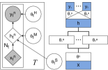
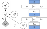
(a)

(b)

Figure 2: Schematics representing our models. In both (a) discriminative model and (b) generative model, $\theta_{S}$ are parameters shared across all task, $\theta^{M}$ are the task specific mask parameters, and $\theta^{H}$ are last layer seperate head parameters. In our exposition, we collectively denote these parameters by $\bm{W}=\bm{B}\odot\bm{V}$ with the masks being $\bm{B}$ and other parameters being $\bm{V}$.

3.1 Generative story

Omitting the task id $t$ for brevity, consider modeling this task using a neural network having $L$ hidden layers. We model the weights in layer $l$ as $\bm{W}^{l}=\bm{B}^{l}\odot\bm{V}^{l}$, a point-wise multiplication of a real-valued matrix $\bm{V}^{l}$ (with a Gaussian prior $\mathcal{N}(0,\sigma_{0}^{2})$ on each entry) and a binary matrix $\bm{B}^{l}$. This ensures sparse connection weights between the layers. Moreover, we model $\bm{B}^{l}\sim\text{IBP}(\alpha)$ using the Indian Buffet Process (IBP) (Griffiths & Ghahramani, 2011) prior, where the hyperparameter $\alpha$ controls the number of nonzero columns in $B$ and its sparsity. The IBP prior thus enables learning the size of $\bm{B}^{l}$ (and consequently of $\bm{V}^{l}$) from data. As a result, the number of node in the hidden layer is learned adaptively from data. The output layer weights are denoted as $\bm{W}_{out}$ with each weight having a Gaussian prior $\mathcal{N}(0,\sigma_{0}^{2})$. The outputs are then assumed to be generated as

$$\bm{y}_{n} \sim\text{Lik}(\bm{W}_{out}\bm{\phi}_{NN}(\bm{x}_{n})),n=1,\ldots,N$$ (2)

Here $\bm{\phi}_{NN}$ is the function computed (using parameter samples) up to the last hidden layer of the network thus formed, and $\operatorname{Lik}$ denotes the likelihood model for the outputs.

Similar priors on the network weights have been used in other recent works to learn sparse deep neural networks (Panousis et al., 2019; Xu et al., 2019). However, these works assume a single task to be learned. In contrast, our focus here is to leverage such priors in the continual learning setting where we need to learn a sequence of tasks, while avoiding the problem of catastrophic forgetting.

Henceforth, we further suppress the superscript denoting layer number from the notation for simplicity; the discussion will hold identically for all hidden layers.

When adapting to a new task in our continual learning setting, the posterior of $\bm{V}$ learnt from previous tasks is used as the prior. A new $\bm{B}$ is learnt afresh, to ensure that a task only learns the subset of weights relevant to it. As described before, to adaptively infer the number of nodes in each hidden layer, we use the IBP prior (Griffiths & Ghahramani, 2011), whose truncated stick-breaking process (Doshi et al., 2009) construction for each entry of $B$ is as follows

$$\nu_{k} \sim\text{Beta}(\alpha,1),\quad\pi_{k}=\prod_{i=1}^{k}\nu_{i}$$ (3)

$$B_{d,k} \sim\text{Bernoulli}(\pi_{k})$$ (4)

for $d\in 1,...,D$, where $D$ denotes the number of input nodes for this hidden layer, and $k\in 1,2,...,K$, where $K$ is the truncation level and $\alpha$ controls the effective value of $K$, i.e., the number of active hidden nodes. Note that the prior probability $\pi_{k}$ of weights incident on hidden node $k$ being nonzero decreases monotonically with $k$, until, say, $K$ nodes, after which no further nodes have any incoming edges with nonzero weights from the previous layer, which amounts to them being turned off from the structure. Moreover, due to the cumulative product based construction of the $\pi_{k}$’s, an implicit ordering is imposed on the nodes being used. This ordering is preserved across tasks, and allocation of nodes to a task follows this, facilitating reuse of weights.

The truncated stick-breaking approximation is a practically plausible and intuitive solution for continual learning, since a fundamental tenet of continual learning is that the model complexity should not increase in an unbounded manner as more and more tasks are encountered. Suppose we fix a budget on the maximum allowed size of the network (say, the number of hidden nodes allowed in each layer) after it has seen, say, $T$ tasks. This exactly corresponds to the truncation level for each layer. Then for each task, nodes are allocated conservatively from this total budget, in a fixed order, conveniently controlled by the $\alpha$ hyper parameter. In Sec. 4.6, we also discuss a dynamic expansion scheme that avoids specifying a truncation level.

3.2 Inference

Exact inference is intractable in this model due to non-conjugacy. Therefore, we resort to variational inference (Blei et al., 2017). We employ structured mean-field approximation (Hoffman & Blei, 2015), which performs better than normally used mean-field approximation, as the former captures the dependencies in the approximate posterior distributions of $\bm{B}$ and $\bm{\nu}$. In particular, we use

$$q(\bm{V},\bm{B},\bm{v})=q(\bm{V})q(\bm{B}|v)q(\bm{v})$$ (5)

where, $q(\bm{V})=\prod_{d=1}^{D}\prod_{k=1}^{K}\mathcal{N}(V_{d,k}|\mu_{d,k},\sigma_{d,k}^{2})$ is a mean field Gaussian approximation for the weights. Corresponding to the Beta-Bernoulli hierarchy of (3), we use the conditionally factorized variational posterior family , that is, $q(\bm{B}|v)=\prod_{d=1}^{D}\prod_{k=1}^{K}\operatorname{Bern}(B_{d,k}|\theta_{d,k})$, where $\theta_{d,k}=\sigma(\rho_{d,k}+logit(\pi_{k}))$ and $q(\bm{v})=\prod_{k=1}^{K}\operatorname{Beta}(v_{k}|\nu_{k,1},\nu_{k,2})$

Thus we have $\Theta=\{\nu_{k,1},\nu_{k,2},\{\mu_{d,k},\sigma_{d,k},\rho_{d,k}\}_{d=1}^{D}\}_{k=1}^{K}$ as the complete set of learnable variational parameters.

Each column of $\bm{B}$ represents the binary mask for the weights incident to a particular node. Note that although these binary variables (in a single column of $\bm{B}$) share a common prior, the posterior for each of these variables is different, thereby allowing a task to selectively choose a subset of the weights leading to an activation, with the common prior controlling the degree of sparsity.

Bayes-by-backprop (Blundell et al., 2015) is a common choice for performing variational inference in this context. The Evidence Lower Bound (ELBO) can be expressed via the data-dependent likelihood and data-independent KL terms

$$\mathcal{L}= \ \mathbb{E}_{q(\bm{V},\bm{B},\bm{v})}[\ln p(\bm{Y}|\bm{V},\bm{B},\bm{v})]$$

$$-KL(q(\bm{V},\bm{B},\bm{v})||p(\bm{V},\bm{B},\bm{v}))$$ (6)

Using the factorization of the joint prior $p(\bm{V},\bm{B},\bm{v})=p(\bm{V})p(\bm{B}|\bm{v})p(\bm{v})$ and the mean-field factorization of the posterior, the KL divergence term of (3.2) decomposes as

$$KL[q(\bm{V})||p(\bm{V})] +\mathbb{E}_{q(\bm{v})}[KL[q(\bm{B}|\bm{v})||p(\bm{B}|\bm{v})]]$$

$$+KL[q(\bm{v})||p(\bm{v})]$$ (7)

All the KL divergence terms in the above expression have closed form expressions; hence using them directly rather than estimating them from Monte Carlo samples alleviates the approximation error as well as the computational overhead due to sampling, to some extent. The expectation terms are optimized by unbiased gradients from the respective posteriors. Using Bayes-by-backprop, we thus have

$$\mathcal{L}= \frac{1}{S}\sum_{i=1}^{S}[f_{l}(\bm{V}^{i},\bm{B}^{i},\bm{v}^{i})-KL[q(\bm{B}|\bm{v}^{i})||p(\bm{B}|\bm{v}^{i})]]$$

$$-KL[q(\bm{V})||p(\bm{V})]-KL[q(\bm{v})||p(\bm{v})]$$ (8)

The log-likelihood term is decomposed as

$$f_{l}(\bm{V},\bm{B},\bm{v}) =\log\operatorname{Lik}(\bm{Y}|\bm{V},\bm{B},\bm{v})$$ (9)

$$=\log\operatorname{Lik}(\bm{Y}|\bm{W}_{out}\bm{\phi}_{NN}(\bm{X;V,B,v}))$$

where $(\bm{X},\bm{Y})$ is the training data. For regression, $\operatorname{Lik}$ can be Gaussian with some noise variance, while for classification it can be Bernoulli with a probit or logistic link.

Sampling details

We obtain unbiased reparameterized gradients for all the parameters of the variational posterior distributions. For the Bernoulli distributed variables, we employ the Gumbel-softmax trick (Jang et al., 2017), also known as CONCRETE (Maddison et al., 2017). For Beta distributed $v$’s, the Kumaraswamy Reparameterization Gradient technique (Nalisnick & Smyth, 2016) is used. For the real-valued weights, the standard location-scale trick of Gaussians is used. The Supplementary Material contains detailed equations.

3.3 Unsupervised Continual Learning

Our discussion thus far has primarily focused on continual learning where each task is a supervised learning problem. Our framework however readily extends to unsupervised continual learning (Nguyen et al., 2018; Smith et al., 2019; Rao et al., 2019) where we assume that each task involves learning a deep generative model, commonly a VAE (Nguyen et al., 2018; Smith et al., 2019; Rao et al., 2019). In this case, each input observation $\bm{x}_{n}$ has an associated latent variable $\bm{z}_{n}$. Collectively denoting all inputs as $\bm{X}$ and all latent variables as $\bm{Z}$, we can define an ELBO similar to Eq. 3.2 as follows :

$$\mathcal{L}= \ \mathbb{E}_{q(\bm{Z},\bm{V},\bm{B},\bm{v})}[\ln p(\bm{X}|\bm{Z},\bm{V},\bm{B},\bm{v})]$$

$$-KL(q(\bm{Z},\bm{V},\bm{B},\bm{v})||p(\bm{Z},\bm{V},\bm{B},\bm{v}))$$ (10)

Note that, unlike the supervised case, the above ELBO also involves an expectation over $\bm{Z}$. Similar to Eq. 8 this can be approximated using Monte Carlo samples, where each ${\bm{z}}_{n}$ is sampled from the amortized posterior $q({\bm{z}}_{n}|\bm{V},\bm{B},\bm{v},{\bm{x}}_{n})$. In addition to learning the model size adaptively, as shown in the schematic diagram (Fig. 2 (b)), our model learns shared weights and task-specific masks for the encoder and decoder models. In contrast, VCL (Nguyen et al., 2018) uses fixed-sized model and entirely task-specific encoders (and of pre-defined sizes), which prevents knowledge transfer across the different encoders.

4 Other Key Considerations

In continual learning setting where the goal is to learn a sequence of tasks, a few other aspects deserve additional consideration. In this section, we discuss how we incorporate them in the context of our proposed model.

4.1 Masked Priors

Using previous task’s posterior as the prior for current task (Nguyen et al., 2018) may be problematic in some cases. For example, the partially learned parameters that do not contribute to previous task may not be useful to be part of the prior for the current task. In fact, instead of forward transfer, using them as prior for next task might even promote catastrophic forgetting. To overcome this issue, we mask the new prior for next task with initial prior as

$$p_{t}(\bm{V}_{d,k}) =B_{d,k}^{o}q_{t-1}(\bm{V}_{d,k})+(1-B_{d,k}^{o})p_{0}(\bm{V}_{d,k})$$ (11)

where ${\bm{B}}^{o}$ is the overall combined mask from all previously learnt tasks i.e., (${\bm{B}}^{1}\cup{\bm{B}}^{2}...\cup{\bm{B}}^{t-1}$), $q_{t-1},p_{t}$ are the previous posterior and current prior, respectively, and $p_{0}$ is the prior used for first task. This makes sense as the partially trained weights will cause undesirable regularization for next task as it does not help retaining the previous tasks performance. Standard choices of initial prior $p_{0}$, such as a zero mean normal distribution or uniform distribution with this masking, further reduces the catastrophic forgetting by promoting the use of new weights or weights with higher variance in previously learned tasks.

4.2 Segregating the head

It has been shown in prior work on supervised continual learning (Zeno et al., 2018) that using separate last layers (commonly referred to as “heads”) for different tasks dramatically improves performance in continual learning. Therefore, in the supervised setting, we use a generalized linear model that uses the embeddings from the last hidden layer, with the parameters up to the last layer involved in transfer and adaptation.

4.3 Prediction-driven training with coresets

Proposed in (Nguyen et al., 2018) as a method for cleverly sidestepping the issue of catastrophic forgetting, the coreset comprises representative training data samples from all tasks. Let $M^{(t-1)}$ denote the posterior state of the model before learning task $t$. With the $t$-th task’s arrival having data $D_{t}$, a coreset $C_{t}$ is created comprising choicest examples from tasks $1\dots t$. Using data $D_{t}\setminus C_{t}$ and having prior $M^{(t-1)}$, new model posterior $M^{t}$ is learnt. For predictive purposes at this stage (the test data comes from tasks $1\dots t$), a new posterior $M^{t}_{pred}$ is learnt with $M^{t}$ as prior and with data $C_{t}$. Note that $M^{t}_{pred}$ is used only for predictions at this stage, and does not have any role in the subsequent learning of, say, $M^{(t+1)}$. Such a predictive model is learnt after every new task, and discarded thereafter. Intuitively it makes sense as some new learnt weights for future tasks can help the older task to perform better (backward transfer) at testing time. For more details, please refer to Appendix C.

During the coreset-based training phase after task $t$, we only update the weights for the tasks $1,\dots,t-1$ with (and using) the binary mask fixed at its previously learned value, i.e., a task refines only its own subset of weights.

4.4 The IBP hyperparameter $\alpha$

Although we found using a sufficiently large value of $\alpha$ without tuning to perform reasonably, we also considered using a schedule with $\alpha$ increasing gradually, and the possibility of learning $\alpha$. We discuss the further details in the Supplementary Material.

4.5 Other Practical issues

Space complexity

The proposed scheme entails storing a binary matrix for each layer of each task which results into 1 bit per weight parameter, which is not very prohibitive and can be efficiently stored/compressed in sparse matrices. Moreover, the initial tasks make use of only a limited number of the first few columns of the IBP matrix, and hence does not pose any significant overhead.

Adjusting bias terms

The IBP selection acts on the weight matrix only. For the hidden nodes not selected in a task, their corresponding biases need to be removed as well. In principle, the bias vector for a hidden layer should be multiplied by a binary vector $\bm{u}$, with $u_{i}=\mathbb{I}[\exists d:B_{d,i}=1]$. In practice, we simply scale each bias component by the maximum reparameterized Bernoulli value in that column.

Selective Finetuning

While training with reparameterization (Gumbel-softmax), the learnt masks are close to binary but not completely binary which affects task performance a bit. So we fine-tune the network with fixed structure (i.e Beta-Bernoulli distributions parameters are fixed) after it has been learned, to restore the accuracy of the task.

4.6 Dynamic Expansion

Although our inference scheme uses a truncation-based approach for the IBP posterior, it is possible to do inference in a truncation-free manner. One possibility is to greedily increase layer width until performance saturates. However we empirically found that this leads to a bad optima. We can leverage the fact that, given a sufficiently large number of columns, the last columns of the IBP matrix tends to be all zeros. So we increase the number of hidden nodes after every iteration to keep the number of such empty columns equal to a constant value $\mathcal{T}^{l}$ in following manner.

$$C_{j}^{l}=C_{j+1}^{l}\prod_{i}^{D^{l}}\mathbb{I}(B_{ij}^{l}=0),\quad G^{l}=\mathcal{T}^{l}-\sum_{j=1}^{K^{l}}C_{j}^{l}$$ (12)

where $l$ represents current layer index, $B^{l}$ is the sampled IBP mask for current task, $C_{j}^{l}$ indicates if all columns from $j^{th}$ column onward are empty. $G^{l}$ is the number of hidden units to expand in the current network layer.

5 Related Work

One of the key challenges in continual learning (henceforth referred to as CL) is to prevent catastrophic forgetting, typically addressed through regularization of the parameter updates, preventing them from drastically changing from the value learnt from the previous task(s). Notable methods based on this strategy include EwC (Kirkpatrick et al., 2017), SI (Zenke et al., 2017), Laplace approximation (Smola et al., 2003), etc. Superceding these methods is the Bayesian approach, a natural remedy of catastrophic forgetting in that, for any task, the posterior of the model learnt from the previous task serves as the prior for the current task, which is the canonical online Bayes. This approach is utilized in recent works like VCL (Nguyen et al., 2018) and task agnostic variational Bayes (Zeno et al., 2018) for learning Bayesian neural networks in the CL setting. Our work is most similar in spirit to and builds upon this body of work.

Another key aspect in CL methods is replay, where some samples from previous tasks (selected randomly or by some heuristic) are used to fine-tune the model after learning a new task (thus refreshing its memory in some sense and avoiding catastrophic forgetting). Some of the works using this idea include (Lopez-Paz et al., 2017), which solves a constrained optimization problem at each task, the constraint being that the loss should decrease monotonically on a heuristically selected replay buffer; (Hu et al., 2018), which uses a partially shared parameter space for inter-task transfer and generates the replay samples through a data-generative module; and (Titsias et al., 2019), which learns a Gaussian process for each task, with a shared mean function in the form a feedforward neural network, the replay buffer being the set of inducing points typically used to speed up GP inference. For VCL (Nguyen et al., 2018) and our work, the coreset (section 4.3) serves as a replay buffer; but we emphasize that it is not the primary mechanism to overcome catastrophic forgetting in these cases, but rather an additional mechanism to preventing it.

Recent work in CL has investigated allowing the structure of the model to dynamically change with newly arriving tasks. Among these, strong evidence in support of our assumptions can be found in (Golkar et al., 2019), which also learns different sparse subsets of the weights of each layer of the network for different tasks. The sparsity is enforced by a combination of weighted $L_{1}$ regularization and threshold-based pruning. There are also methods that do not learn subset of weights to be used but rather learn the subset of hidden layer node outputs to be used for each task; such a strategy is adopted by either using Evolutionary Algorithms to select the node subsets (Fernando et al., 2017) or by training the network with task embedding based attention masks (Serrà et al., 2018). One recent approach (Adel et al., 2019), instead of using binary masks, tries to adapts weights at different scales for different tasks; it is also designed only for discriminative tasks.

Among other related work, (Li et al., 2019; Yoon et al., 2018; Xu & Zhu, 2018) either reuse the parameters of a layer, dynamically grows the size of the hidden layer, or adapt them, or spawn a new set of parameters (the model complexity being bounded through regularization terms or reward based reinforcements). Most of these approaches however tend to be rather expensive and rely on techniques, such as neural architecture search. In another recent work (simultaneous development with our work), (Kessler et al., 2019) did a preliminary investigation on using IBP for continual learning. They however use IBP on hidden layer activations instead of weights (which they mention is worth considering), do not consider issues such as the ones we discussed in Sec. 4, and only considered the supervised setting.

6 Experiments

We perform experiments on both supervised and unsupervised CL and compare our method with relevant state-of-the-art methods. In addition to the quantitative (accuracy/log-likelihood comparisons) and qualitative (generation) results, we also examine the network structures learned by our model. Some of the details (e.g., experimental settings) have been moved to the Supplementary Material.

6.1 Supervised Continual Learning

We first evaluate our model on standard supervised CL benchmarks. We experiment with different existing approaches such as, Pure Rehearsal (Robins, 1995), EwC (Kirkpatrick et al., 2017), IMM (Lee et al., 2017), DEN (Yoon et al., 2018), RCL (Xu & Zhu, 2018), and “Naïve” which learns a shared model for all the tasks.

We perform our evaluations on three supervised CL benchmark datasets: SplitMNIST, Split notMNIST(small), Permuted MNIST and fashion MNIST. For Split MNIST, the tasks consist of 5 binary classification problems, the splits being 0/1, 2/3, 4/5, 6/7, 8/9 digits. Split notMNIST consists of 5 binary classification splits as A/B, C/D, E/F, G/H, I/J and, similarily, fashionMNIST consists of 5 binary classification splits as T-shirt/Trouser, Pullover/Dress, Coat/Sandals, Shirt/Sneaker, and Bag/Ankle boots. For Permuted MNIST, each task is a multiclass classification problem. However, for each task, a fixed random permutation is applied to the pixels of the images of all classes. We generated 5 such tasks for our experiments. The heads are separate for different tasks (Sec. 4.2).

6.1.1 Performance evaluation

Suppose we have $T$ tasks arriving sequentially. To gauge the effectiveness of our model towards preventing catastrophic forgetting, we report ($i$) the test accuracy of task $t$ after learning each of the subsequent tasks ($t,t+1,t+2,\dots T$); and ($ii$) the average test accuracy over all previous tasks $1,2,\dots t$ after learning each task $t$.

We use a feed-forward network (ReLU activations) with a single hidden layer having total budget of 200 nodes. For fair comparison, we use the same architecture for each of the baselines, except for DEN and RCL that grows the structure with two hidden layers. We also report results on some additional CL metrics (Díaz-Rodríguez et al., 2018) in the Supplementary Material.

Quantitative Results:

Fig. 3 shows the mean test accuracies on splitMNIST, notMNIST, permuted MNIST, and fashion MNIST as new tasks are observed. As Fig. 3 shows, the average test accuracy of our method (without as well as with coresets) is better than the other baseline (here, we have used random point selection method for coresets). Moreover, the accuracy drops much more slowly than and other baselines showing the efficacy of our model in preventing catastrophic forgetting due to the adaptively learned structure. In Fig. 4, we show the accuracy on individual tasks (for tasks 1-4) as new tasks arrive and compare specifically with VCL. In this case too, we observe that our method yields relatively stable individual task accuracies as compared to VCL. Also, as with VCL, using coreset was found to improve performance a bit. We also note that some of the old tasks’ accuracies increases with training of new tasks which shows the presence of backward transfer, which is another desideratum of CL. We also report the performance with dynamic expansion of network initialized to 50 hidden units; it performs slightly worse than the truncation-based method but better than the other methods.

One further observation is that, for VCL, while the individual test accuracies improve with more training on each task, the overall performance across all tasks drops gradually, possibly since more training on a single task adapts the model more specifically for that task, leading to forgetting of the previous tasks. Our model, on the other hand, was found to be immune to over-training, since each task learns its own sparse subset of parameters.

Figure 3: Mean test accuracies of tasks seen so far as new tasks are observed, for (a)splitMNIST, (b)notMNIST , (c)Permuted MNIST and (d) fashionMNIST, here (right) side plots are scaled version of (left) ones for better insight

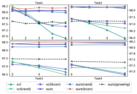
Figure 4: Comparison with VCL : Test accuracy of tasks 1, 2, 3, 4 (left to right) as newer tasks are observed for Permuted MNIST, random and k-center are methods used for coreset selection

Figure 5: Sequential generation for MNIST and notMNIST datasets (Supp. Material contains more illustrations and zoomed-in versions).

6.2 Unsupervised Continual Learning

We next evaluate our model for generative tasks under CL setting. For this evaluation, compare our model with existing approaches such as Naïve, EwC (Kirkpatrick et al., 2017) and VCL (Nguyen et al., 2018). We do not include other methods mentioned in supervised setup as their implementation does not incorporate generative modeling.

We perform continual learning experiments for deep generative models using a VAE style network. We consider two datasets, MNIST and notMNIST (small). For MNIST, the tasks are sequence of single digit generation from 0 to 9. Similarily, for notMNIST we define each task as one character generation from A to J.

Note that, unlike VCL and other baselines where all tasks have separate encoder and a shared decoder with separate head for latent dimension, as we discuss in Sec. 3.3, our model uses a shared encoder for all tasks, but with task-specific masks for each encoder (cf., Fig. 2 (b)). This enables transfer of knowledge while the task-specific mask effectively prevent catastrophic forgetting.

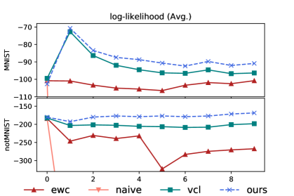
Figure 6: Log-likelihoods of benchmarks on generative tasks.

6.2.1 Performance evaluation

Generation: As shown in Fig  6, the modeling innovation we introduce for the unsupervised setting, indeed results in much improved log-likelihood on held-out sets. We also observe that the quality of generated samples in Fig  5 does not deteriorate as compared to other baselines as more and more tasks are encountered. In each individual figure in Fig  5, each row represents the generated samples from all previously seen tasks and the current task. This shows that our model can efficiently perform generative modeling by reusing subset of networks and creating minimal number of nodes for each task.

Representation Learning: We also perform an experiment to assess the quality of the unsupervisedly learned representation by our unsupervised continual learning approach. For this experiment, we use the learned representations to train a classification model. Due to space limitation, the details of this experiment are provided in the Supplementary Material.

6.3 Some Structural Observations

An appealing aspect of our work is that, the results reported above, which are competitive with the state-of-the-art, are achieved with a very sparse neural network structures learnt by the model, which we analyze qualitatively here (the Supplementary Material shows some examples of network structures learnt by our model).

Further, as expected by proposed model, as shown in Fig. 7 (b), the IBP prior enforces the weights to be concentrated mainly on the first few nodes, and the structure results in a sparse network. For both notMNIST and Permuted MNIST datasets, a maximum of around 15% incoming connections are used at most for the first task.

Another important observation (as shown in Fig. 7 (a)) is the percentage of weights that are being shared between different tasks and how the number of active weights vary across different tasks based on their similarities. Qualitatively, it appears that most newer tasks tend to allocate fewer weights and yet perform well, implying effective forward transfer. One can also easily observe that the weight sharing between similar tasks like those in notMNIST is a much higher than that of non-similar tasks such as permuted MNIST. This seemingly leads to the hypothesis that a single binary mask common for all tasks is sufficient. Experimental observations, however, dispel such a belief by showing drastic degradation in performance.

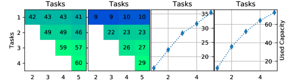
(a)

(b)

Figure 7: Percentage of weight sharing across tasks (a), percentage of network filled or used after learning k tasks (b), the first and third plots are from notMNIST results and the second and fourth plots are fromr permuted MNIST results

We therefore conclude that although a new task tend to share weights learnt by old tasks, the new connections that it creates are indispensable for its performance. Intuitively, the more unrelated a task is to previously seen ones, the more new connections it will make, thus reducing negative transfer (an unrelated task adversely affecting other tasks) between tasks.

7 Conclusion

We have successfully unified structure learning in neural networks with their variational inference in the setting of continual learning, demonstrating competitive performance with state-of-the-art models on both discriminative (supervised) and generative (unsupervised) learning problems. It would also be interesting to extend this idea to more sophisticated network architectures such as convolutional or residual networks, possibly by also exploring improved approximate inference methods. Another interesting extension would be for semi-supervised continual learning. Adapting other sparse Bayesian structure learning methods, e.g. (Ghosh et al., 2018) to the continual learning setting is also a promising avenue. Adapting the depth of the network is a more challenging endeavour that might also be undertaken. We leave these extensions for future work.

A Data

The data sets used in our experiments with train test split information are listed in table given below. MNIST dataset comprises $28\times 28$ monochromatic images consisting of handwritten digits from 0 to 9. notMNIST dataset comprises of glyph’s of letters A to J in different fonts formats with similar configuration as MNIST. fashion MNIST is also monochromatic comprising of 10 classes (T-shirt, Trouser, Pullover, Dress, Coat, Sandal, Shirt, Sneaker, Bag, Ankle boot) with similar to MNIST.

Dataset	Classes	Training size	Test size
MNIST	10	60000	10000
notMNIST	10	14974	3750
fashionMNIST	10	50000	20000

B Model Configurations

For permuted MNIST, split MNIST, split notMNIST and fashion MNIST experiments, we use fixed architecture of network for all the models with single hidden layer of 200 units except for DEN (which grows structure dynamically) which used two hidden layers initialized to $256,128$ units.

The VCL implementation was taken directly from their official repository at https://github.com/nvcuong/variational-continual-learning. For DEN we used the official implementation at https://github.com/jaehong-yoon93/DEN. IMM implementation was taken from https://github.com/btjhjeon/IMM_tensorflow, RCL implementation was taken from https://https://github.com/xujinfan/Reinforced-Continual-Learning, For EwC we used HAT’s official implementation at https://github.com/joansj/hat. For rest of the models, we used our own implementations.

B.1 Supervised Continual Learning: Hyperparameter settings

For all datasets, our model uses single hidden layer neural network with $200$ hidden units. For RCL (Xu & Zhu, 2018) and DEN (Yoon et al., 2018), two hidden layers were used with initial network size of $256,128$ units, respectively. We adopt Adam optimizer for our model keeping a learning rate of $0.01$ for the IBP posterior parameters and $0.001$ for others; this is to avoid vanishing gradient problem introduced by sigmoid function. For selective finetuning, we use a learning rate of $0.0001$ for all the parameters. The temperature hyperparameter of the Gumbel-softmax reparameterization for Bernoulli gets annealed from 10.0 to a minimum limit of 0.25. The value of $\alpha$ is initialized to 30.0 for the initial task and maximum of the obtained posterior shape parameters for each of subsequent tasks. Similar to VCL, we initialize our models with maximum-likelihood training for the first task. For all datasets, we train our model for 5 epochs. We selectively finetune our model after that for 5 epochs. For experiments including coresets, we use a coreset size of 50. Coreset selection is done using random and $k$-center methods (Nguyen et al., 2018). For our model with dynamic expansion, we initialize our network with 50 hidden units.

B.2 Unsupervised Continual Learning: Hyperparameter settings

For all datasets, our model uses 2 hidden layers with $500,500$ units for encoder and symmetrically opposite for the decoder with a latent dimension of size $100$ units. For other approaches like Naive, EwC and VCL (Kirkpatrick et al., 2017; Nguyen et al., 2018), we use task-specific encoders with 3 hidden layers of $500,500,500$ units respectively with latent size of $100$ units, and a symmetrically reversed decoder with last two layers of decoder being shared among all the tasks and the first layer being specific to each task. we use Adam optimizer for our model keeping the learning rate configuration similar to that of supervised setting. Temperature for gumbel-softmax reparametrization gets annealed from 10 to 0.25. We initialize encoder hidden layers $\alpha$ values as $40,40$, respectively, and symmetrically opposite in decoder for the first task. We update $\alpha$’s in similar fashion to supervised setting for subsequent tasks. For latent layers, we intialize $\alpha$ to $20$. For the unsupervised learning experiments, we did not use coresets.

Algorithm 1 Nonparametric Bayesian CL

  Input:Initial Prior $p_{0}(\Theta)$

  Initialize the network parameters and coresets

  Initialize : $p_{new}\leftarrow p_{0}(\Theta)$

  for $i=1$ to $T$ do

     Observe current task data $D_{t}$ 

     Update coresets (Appendix C) 

     Masked Training 

        $\mathcal{L}_{t}\leftarrow$ ELBO (Eq. 6) with prior $p_{new}$ 

        $\Theta_{t}\leftarrow\arg\min\mathcal{L}_{t}$ 

     Selective Finetuning 

        Fix the IBP parameters and learned mask 

        $\Theta_{t}\leftarrow\arg\min\mathcal{L}_{t}$ 

     $p_{new}\leftarrow q_{t}(\Theta)$ 

     $p_{new}\leftarrow$ Mask($p_{new}$) using Eq 11 

     Perform prediction for given test set..

  end for

C Coreset Method Explanation

As done in VCL (Nguyen et al., 2018), for each task, a new coreset is produced by selecting a few points from the new task and the old coreset. Coreset selection can be done either through random selection or $K$-center greedy algorithm  (Gonzalez, 1985). Next, the posterior is decomposed as follows:

$$p(\theta|D_{1:t})\propto p(\theta|D_{1:t}\char 92\relax C_{t})p(C_{t}|\theta)\approx\tilde{q}_{t}(\theta)p(C_{t}|\theta)$$

where, $q(\theta)$ is the variational posterior obtained using the current task training data, excluding the current coreset data. Applying this trick in a recursive fashion, we can write:

$$p(\theta|D_{1:t}\char 92\relax C_{t}) =p(\theta|D_{1:t-1}\char 92\relax C_{t-1})p(D_{t}\cup C_{t-1}\char 92\relax C_{t}|\theta)$$

$$\approx\tilde{q}_{t-1}(\theta)p(D_{t}\cup C_{t-1}\char 92\relax C_{t}|\theta)$$

We then approximate this posterior using variational approximation as $\tilde{q}_{t}(\theta)=proj(\tilde{q}_{t-1}(\theta)p(D_{t}\cup C_{t-1}\char 92\relax C_{t}|\theta))$ Finally a projection step is performed using coreset data before prediction as follows: $q_{t}(\theta)=proj(\tilde{q}_{t}(\theta)p(C_{t}|\theta))$. This way of incorporating coresets into coreset data before prediction tries to mitigate any residual forgetting. Algorithm 1 summarizes the training procedure for our model.

D Additional Inference Details

Inference over parameters $\phi$ that involves a random or stochastic node $Z$ (i.e $Z\sim q_{\phi}(Z)$) cannot be done in a straightforward way, if the objective involves Monte Carlo expectation with respect that random variable $(\mathcal{L}=\mathbb{E}_{q_{\phi}{z}}(L(z))))$. This is due to the inability to back-propagate through a random node. To overcome this issue, (Kingma & Welling, 2013) introduced the reparametrization trick. This involves deterministically mapping the random variable $Z=f(\phi,\epsilon)$ to rewrite the expectation in terms of new random variable $\epsilon$, where $\epsilon$ is now randomly sampled instead of $Z$ (i.e $\mathcal{L}=\mathbb{E}_{q{\epsilon}}[L(\epsilon,\phi)]$). In this section, we discuss some of the reparameterization tricks we used.

D.1 Gaussian distribution Reparameterization

The weights of our Bayesian nueral network are assumed to be distributed according to a Gaussian with diagonal variances (i.e $V_{k}\sim\mathcal{N}(V_{k}|\mu_{V_{k}},\sigma^{2}_{V_{k}})$). We reparameterize our parameters using location-scale trick as:

$$V_{k}=\mu_{V_{k}}+\sigma_{V_{k}}\times\epsilon,\quad\epsilon\sim\mathcal{N}(0,I)$$

where $k$ is the index of parameter that we are sampling. Now, with this reparameterization, the gradients over $\mu_{V_{k}},\sigma_{V_{k}}$ can be calculated using back-propagation.

D.2 Beta distribution Reparameterization

The beta distribution for parameters $\nu$ in the IBP posterior can be reparameterized using Kumaraswamy distribution (Nalisnick & Smyth, 2016), since Kumaraswamy distribution and beta distribution are identical if any one of rate or shape parameters are set to 1. The Kumaraswamy distribution is defined as $p(\nu;\alpha,\beta)=\alpha\beta\nu^{\alpha-1}(1-\nu^{\alpha})^{\beta-1}$ which can be reparameterized as:

$$\nu=(1-u^{1/\beta})^{1/\alpha},\quad u\sim U(0,1)$$

where $U$ represents a uniform distribution. The KL-Divergence between Kumaraswamy and beta distributions can be written as:

$$KL(q(\nu;a,b)|| p(\nu;\alpha,\beta))=\frac{a-\alpha}{a}\left(-\gamma-\Psi(b)-\frac{1}{b}\right)$$

$$+\log{ab}+\log(B(\alpha,\beta))-\frac{b}{1-b}$$

$$+(\beta-1)b\sum_{m=1}^{\infty}\frac{1}{m+ab}B(\frac{m}{a},b)$$ (13)

where $\gamma$ is the Euler constant, $\Psi$ is the digamma function and B is the beta function. As described in (Nalisnick & Smyth, 2016), we can approximate the infinite sum in Eq.13 with a finite sum using first 11 terms.

D.3 Bernoulli distribution Reparameterization

For Bernoulli distribution over mask in the IBP posterior, we employ the continuous relaxation of discrete distribution as proposed in Categorical reparameterization with Gumbel-softmax (Jang et al., 2017), also known as the CONCRETE (Maddison et al., 2017) distribution. We sample a concrete random variable from the probability simplex as follows:

$$B_{k}=\frac{\exp((\log(\alpha_{k})+g_{k})/\lambda)}{\sum^{K}_{i=1}\exp((\log(\alpha_{i})+g_{i})/\lambda)},\quad g_{k}\sim G(0,1)$$

where, $\lambda\in(0,\infty)$ is a temperature hyper-parameter, $\alpha_{k}$ is posterior parameter representing the discrete class probability for $k^{th}$ class and $g_{k}$ is a random sample from Gumbel distribution $G$. For binary concrete variables, the sampling reduces to the following form:

$$Y_{k}=\frac{\log{(\alpha_{k})}+\log{(u_{k}/(1-u_{k}))}}{\lambda},\quad u\sim U(0,1)$$

then, $B_{k}=\sigma(Y_{k})$ where $\sigma$ is sigmoid function and $u_{k}$ is sample from uniform distribution U. To guarantee a lower bound on the ELBO, both prior and posterior Bernoulli distribution needs to be replaced by concrete distributions. Then the KL-Divergence can be calculated as difference of log density of both distributions. The log density of concrete distribution is given by:

$$\log q(B_{k};\alpha,\lambda) =\log{(\lambda)}-\lambda Y_{k}+\log{\alpha_{k}}$$

$$-2\log{(1+\exp{(-\lambda Y_{k}+\log{\alpha_{k}})})}$$

With all reparameterization techniques discussed above, we use Monte Carlo sampling for approximating the ELBO with sample size of 10 while training and a sample size of 100 while at test time.

E IBP Hyperparameter $\alpha$

In this section, we discuss the approach to tune the IBP prior hyperparameter $\alpha$. As discussed earlier, we found that using a sufficiently large value of $\alpha$ without tuning performs reasonably well in practice. However, we experimented with other alternatives as well. For example, we tried adapting $\alpha$ with respect to previous posterior as $\alpha=max(\alpha,max(a_{\nu}))$ for each layer, where $a_{\nu}$ is Beta posterior shape parameter. Several other considerations can also be made regarding its choice.

E.1 Scheduling across tasks

Intuitively, $\alpha$ should be incremented for every new task according to some schedule. Information about task relatedness can be helpful in formulating the schedule. Smaller increments of $\alpha$ discourages creation of new nodes and encourages more sharing of already existing connections across tasks.

E.2 Learning $\alpha$

Although not investigated in this work, one viable alternative to choosing $\alpha$ by cross-validation could be to learn it. This can be accommodated into our variational framework by imposing a gamma prior on $\alpha$ and using a suitably parameterized gamma variational posterior. The only difference in the objective would be in the KL terms: the KL divergence of $\bm{v}$ will then also have to estimated by Monte Carlo approximation (because of dependency on $\alpha$ in the prior). Also, since gamma distribution does not have an analytic closed form KL divergence, the Weibull distribution can be a suitable alternative (Zhang et al., 2018).

F Additional Results: Supervised Continual Learning

In this section, we provide some additional experimental results for supervised continual learning setup. Table 1 shows final mean accuracies over 5 tasks with deviations, obtained by all the approaches on various datasets. It also shows that our model performs comparably or better than the baselines.

F.1 Learned Network Structures

In this section, we analyse the network structures that were learned after training our model.

Figure 8: Learned masks for input to first hidden layer weights on splitMNIST dataset. Darker color represent active weights.

As we can see in Fig. 8, the masks are captured on the pixel values where the digits in MNIST datasets have high value and zeros elsewhere which represents that our models adapts with respect to data complexity and only uses those weights that are required for the task. Due to the use of the IBP prior, the number of active weights tends to shrink towards the first few nodes of the first hidden layer. This observation enforces that our idea of using IBP prior to learn the model structure based on data complexity is indeed working. Similar behaviour can be seen in notMNIST and fashionMNIST in Fig. 9. On the other hand Fig 10 (left) shows the sharing of weights between subsequent tasks of different datasets. It can be observed that the tasks that are similar at input level of representation have more overlapping/sharing of parameters (e.g split MNIST) in comparison to those that are not very similar (e.g permuted MNIST). It also shows Fig 10 (right) that the amount of total network capacity used by our model differs for each task, which shows that complex tasks require more parameters as compared to easy tasks.

Method	split MNIST	notMNIST	permuted MNIST	fashion MNIST
Naïve	79.615$\pm$0.7	72.339$\pm$0.8	90.090$\pm$0.4	79.319$\pm$0.6
Rehearsal	99.102$\pm$0.3	95.203$\pm$0.5	97.565$\pm$0.3	97.981$\pm$0.3
EwC	81.530$\pm$0.4	90.297$\pm$0.6	95.392$\pm$0.5	86.577$\pm$0.4
IMM (mode)	92.206$\pm$0.6	84.442$\pm$0.4	96.433$\pm$0.5	88.765$\pm$0.4
VCL	98.952$\pm$0.3	93.732$\pm$0.3	97.353$\pm$0.3	97.970$\pm$0.2
VCL(coreset)	98.731$\pm$0.4	94.993$\pm$0.2	97.464$\pm$0.3	98.154$\pm$0.3
DEN	99.779$\pm$0.1	96.485$\pm$0.3	97.945$\pm$0.2	98.580$\pm$0.3
RCL	99.768$\pm$0.1	96.722$\pm$0.2	98.005$\pm$0.2	98.698$\pm$0.2
Ours	99.819$\pm$0.1	97.152$\pm$0.2	98.180$\pm$0.2	98.986$\pm$0.2
Ours(coreset)	99.834$\pm$0.1	97.061$\pm$0.2	98.163$\pm$0.3	98.990$\pm$0.2

Table 1: Comparison of final mean accuracies on test set obtained using different methods. Deviations are rounded to 1 decimal place

Since the network size is fixed, the amount of network usage for all previous tasks tends to converge towards 100 percent. This promotes parameter sharing but also introduces forgetting, since the network is forced to share parameters and is not able to learn new nodes.

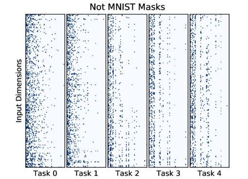
Figure 9: Learned masks for input to first hidden layer weights on notMNIST(top) and fashion MNIST(bottom) datasets. Darker color represent active weights.

F.2 Other Metrics

We quantified and observed the forward and backward transfer of our and VCL model, using the three metrics given in (Díaz-Rodríguez et al., 2018) on Permuted MNIST dataset as follows:

Accuracy

is defined as the overall model performance averaged over all the task pairs as follows:

$$Acc=\frac{\sum_{i\geq j}R_{i,j}}{\frac{N(N-1)}{2}}$$

where, $R_{i,j}$ is obtained test classification accuracy of the model on task $t_{j}$ after observing the last sample from task $t_{i}$.

Figure 10: Percentage weight sharing between tasks (left), percentage of network capacity already used by previous tasks(right).

Forward Transfer

is the ability of previously learnt task to perform on new task better and is give by:

$$FWT=\frac{\sum_{i<j}^{N}R_{i,j}}{\frac{N(N-1)}{2}}$$

Backward Transfer

is the ability of newly learned task to affect the performance of previous tasks. It can be defined as:

$$BWT=\frac{\sum_{i=2}^{N}\sum_{j=1}^{i-1}(R_{i,j}-R_{j,j})}{\frac{N(N-1)}{2}}$$

We compare our model with VCL and other baselines over these three metrics in Table 2.

Method	Acc	FWT	BWT
Naive	$90.090$	$0.1$	$-3.60e^{-2}$
EwC	$95.392$	$0.1$	$-1.90e^{-2}$
Rehearsal	$97.565$	$0.1$	$+1.30e^{-4}$
VCL	$97.353$	$0.1$	$-4.00e^{-3}$
Ours	$98.180$	$0.1$	$+1.33e^{-5}$

Table 2: Comparison on other metrics for permuted MNIST dataset

We can observe that backward transfer for our model is more as compared to most baselines, which shows that our approach has suffers from less forgetting as well. On the other hand forward transfer seems to give close to random accuracy (0.1) which is due to the fact that the model is not trained on the correct class labels and is asked to predict the correct label. So this metric is not very useful here; an alternative would be to train a linear classifier on the representations that are learned after each subsequent tasks for future task.

G Unsupervised Continual Learning

Here we describe the complete generative model for our unsupervised continual learning approach. The generative story for unsupervised setting can be written as follows (for brevity we have omitted the task id $t$):

$$\bm{B}^{l} \sim IBP(\alpha)$$

$$\bm{V}_{d,k}^{l} \sim\mathcal{N}(0,\sigma_{0}^{2})$$

$$\bm{W}^{l} =\bm{B}^{l}\odot\bm{V}^{l}$$

$$\bm{W}^{out}_{d,k} \sim\mathcal{N}(0,\sigma_{0}^{2})$$

$$\bm{Z}_{n} \sim\mathcal{N}(\mu_{z},\sigma_{z}^{2})$$

$$\bm{X}_{n}\sim Bernoulli (\sigma(\bm{W}^{out}\bm{\phi}_{NN}(\bm{W},\bm{Z}_{n})))$$

where, $\mu_{z},\sigma_{z}^{2}$ are prior parameters of latent representation; they can either be fixed or learned, and $\sigma$ is the sigmoid function. The stick-breaking process for the IBP prior remains the same here as well. For doing inference here, once again we resort to structured mean-field assumption:

$$q(\bm{Z},\bm{V},\bm{B},\bm{v})=q(\bm{Z}|\bm{B},\bm{V},\bm{\nu},\bm{X})q(\bm{V})q(\bm{B}|v)q(\bm{v})$$

where, $q(\bm{Z}|\bm{B},\bm{V},\bm{\nu},\bm{X})=\prod_{n=1}^{N}\mathcal{N}(\mu_{\phi_{NN}},\sigma^{2}_{\phi_{NN}})$, and $\phi_{NN}$ is IBP masked neural network used for amortization of Gaussian posterior parameters. Rest of variational posteriors are factorized in a similar way as in the supervised approach. Evidence lower bound calculation can done as explained in section 3.3.

G.1 Additional Experimental Results for Unsupervised Continual Learning

In this section, we show further results for unsupervised continual learning. Fig 12 shows, for MNIST and notMNIST datasets, how the likelihoods vary for individual tasks as subsequent tasks arrive. It can be observed that the individual task accuracies

Figure 11: On MNIST dataset (Top) Reconstruction of images after all tasks have been observed. (Bottom) t-SNE plot of each class after all tasks have been observed.

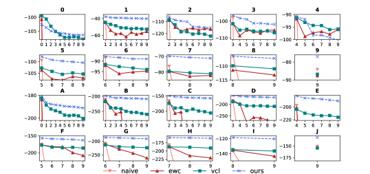
Figure 12: Generative Model : Test likelihood decays of individual tasks after subsequent tasks have been observed. (Top two) represents MNIST and (Bottom two) represents notMnist datasets.

learned by our model are better than other baselines; this suggests that use of new weights when needed helps in retaining a better optima per task, and also the deterioration of our model is much less as compared to other model, representing effective protection against catastrophic forgetting. Fig 11 shows the reconstructed images of MNIST and also the t-SNE plot of latent codes our model produces. it can be observed that reconstruction quality is good despite heavy constraints on the model.

Figure 13: Generated samples on MNIST dataset after all tasks have been observed

Fig 13 shows the generated samples from the learned prior over latent space after all tasks are observed.

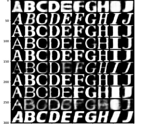
Figure 14: On notMNIST dataset (Top) Reconstruction of images after all tasks have been observed. (Bottom) t-SNE plot of each class after all tasks have been observed.

Figure 15: Generated samples on notMNIST dataset after all tasks have been observed

Similarily, Fig 14 shows the reconstructed images of not MNIST dataset and the t-SNE plot of latent codes our model produces, and Fig 15 shows the generated samples from the learned prior over latent space after all tasks are observed.

Benchmarks	MNIST			not MNIST
	3-KNN error	5-KNN error	10-KNN error	3-KNN error	5-KNN error	10-KNN error
Naive	30.1%	33.1%	36.0%	20.6%	24.87%	30.8%
EwC	16.6%	19.48%	22.3%	11.7%	13.1%	17.8%
VCL	17.0%	19.02%	30.2%	12.3%	13.8%	16.5%
Ours	0.37%	0.40%	0.51%	0.08%	0.09%	0.21%

Table 3: Unsupervised learning benchmark comparison with sampled latents using K-nearest neighbour test.

Representation Learning

In t-SNE plots, it can be observed that the latent space for MNIST dataset is more clearly seperated as compared to notMNIST dataset. This can be attributed to the abundance of data and less variation in MNIST dataset as compared to notMNIST dataset. we further analyzed the representations that were learned by our model by doing $K$-Nearest Neighbour classification on the latent space. Table 3 shows the KNN test error of our model and few other benchmarks on MNIST and notMNIST datasets. We performed the test with three different values for $K$. As shown in the table, the representations learned by other baselines are not very useful (as evidenced by the large test errors), since the latent space are not shared among the tasks, whereas our model uses a shared latent space (yet modulated for each task based on the learned task-specific mask) which results in effective latent representation learning.

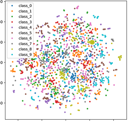
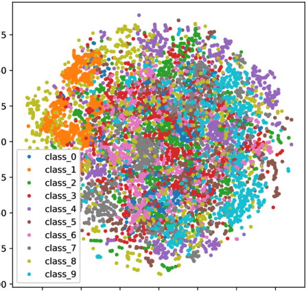
Figure 16: t-SNE plot of latent space of VCL model on notMNIST (top) and MNIST (bottom) datasets

References

- Adel et al. (2019) Adel, T., Zhao, H., and Turner, R. E. Continual Learning with Adaptive Weights (CLAW). arXiv e-prints, art. arXiv:1911.09514, Nov 2019.
- Blei et al. (2017) Blei, D. M., Kucukelbir, A., and McAuliffe, J. D. Variational inference: A review for statisticians. Journal of the American statistical Association, 112(518):859–877, 2017.
- Blundell et al. (2015) Blundell, C., Cornebise, J., Kavukcuoglu, K., and Wierstra, D. Weight uncertainty in neural networks. arXiv preprint arXiv:1505.05424, 2015.
- Díaz-Rodríguez et al. (2018) Díaz-Rodríguez, N., Lomonaco, V., Filliat, D., and Maltoni, D. Don’t forget, there is more than forgetting: new metrics for continual learning. arXiv preprint arXiv:1810.13166, 2018.
- Doshi et al. (2009) Doshi, F., Miller, K., Van Gael, J., and Teh, Y. W. Variational inference for the indian buffet process. In AISTATS, pp. 137–144, 2009.
- Fernando et al. (2017) Fernando, C., Banarse, D., Blundell, C., Zwols, Y., Ha, D., Rusu, A. A., Pritzel, A., and Wierstra, D. Pathnet: evolution channels gradient descent in super neural networks. arXiv: 1701.08734, January 2017.
- Flesch et al. (2018) Flesch, T., Balaguer, J., Dekker, R., Nili, H., and Summerfield, C. Comparing continual task learning in minds and machines. Proceedings of the National Academy of Sciences, 115(44):E10313–E10322, 2018.
- Ghosh et al. (2018) Ghosh, S., Yao, J., and Doshi-Velez, F. Structured variational learning of bayesian neural networks with horseshoe priors. ICML, 2018.
- Golkar et al. (2019) Golkar, S., Kagan, M., and Cho, K. Continual learning via neural pruning. arXiv preprint arXiv:1903.04476, 2019.
- Gonzalez (1985) Gonzalez, T. F. Clustering to minimize the maximum intercluster distance. Theor. Comput. Sci., 38:293–306, 1985.
- Griffiths & Ghahramani (2011) Griffiths, T. L. and Ghahramani, Z. The indian buffet process: An introduction and review. JMLR, 12(Apr):1185–1224, 2011.
- Hoffman & Blei (2015) Hoffman, M. and Blei, D. Stochastic Structured Variational Inference. AISTATS, 38:361–369, 2015.
- Hu et al. (2018) Hu, W., Lin, Z., Liu, B., Tao, C., Tao, Z., Ma, J., Zhao, D., and Yan, R. Overcoming catastrophic forgetting for continual learning via model adaptation. 2018.
- Jang et al. (2017) Jang, E., Gu, S., and Poole, B. Categorical reparameterization with gumbel-softmax. ICLR, 2017.
- Kessler et al. (2019) Kessler, S., Nguyen, V., Zohren, S., and Roberts, S. Indian buffet neural networks for continual learning. arXiv preprint arXiv:1912.02290, 2019.
- Kingma & Welling (2013) Kingma, D. P. and Welling, M. Auto-encoding variational bayes. arXiv preprint arXiv:1312.6114, 2013.
- Kirkpatrick et al. (2017) Kirkpatrick, J., Pascanu, R., Rabinowitz, N., Veness, J., Desjardins, G., Rusu, A. A., Milan, K., Quan, J., Ramalho, T., Grabska-Barwinska, A., et al. Overcoming catastrophic forgetting in neural networks. Proceedings of the national academy of sciences, 114(13):3521–3526, 2017.
- Lee et al. (2017) Lee, S.-W., Kim, J.-H., Jun, J., Ha, J.-W., and Zhang, B.-T. Overcoming Catastrophic Forgetting by Incremental Moment Matching. arXiv e-prints, Mar 2017.
- Li et al. (2019) Li, X., Zhou, Y., Wu, T., Socher, R., and Xiong, C. Learn to grow: A continual structure learning framework for overcoming catastrophic forgetting. arXiv preprint arXiv:1904.00310, 2019.
- Lopez-Paz et al. (2017) Lopez-Paz, D. et al. Gradient episodic memory for continual learning. In NIPS, pp. 6467–6476, 2017.
- Maddison et al. (2017) Maddison, C. J., Mnih, A., and Teh, Y. W. The concrete distribution: A continuous relaxation of discrete random variables. ICLR, 2017.
- Nalisnick & Smyth (2016) Nalisnick, E. and Smyth, P. Stick-Breaking Variational Autoencoders. arXiv e-prints, art. arXiv:1605.06197, May 2016.
- Neal (2012) Neal, R. M. Bayesian learning for neural networks, volume 118. Springer Science & Business Media, 2012.
- Nguyen et al. (2018) Nguyen, C. V., Li, Y., Bui, T. D., and Turner, R. E. Variational continual learning. ICLR, 2018.
- Pan & Yang (2009) Pan, S. J. and Yang, Q. A survey on transfer learning. IEEE Transactions on knowledge and data engineering, 22(10):1345–1359, 2009.
- Panousis et al. (2019) Panousis, K., Chatzis, S., and Theodoridis, S. Nonparametric bayesian deep networks with local competition. In International Conference on Machine Learning, pp. 4980–4988, 2019.
- Parisi et al. (2019) Parisi, G. I., Kemker, R., Part, J. L., Kanan, C., and Wermter, S. Continual lifelong learning with neural networks: A review. Neural Networks, 2019.
- Rao et al. (2019) Rao, D., Visin, F., Rusu, A., Pascanu, R., Teh, Y. W., and Hadsell, R. Continual unsupervised representation learning. In Advances in Neural Information Processing Systems, pp. 7645–7655, 2019.
- Ring (1997) Ring, M. B. Child: A first step towards continual learning. Machine Learning, 28(1):77–104, 1997.
- Robins (1995) Robins, A. Catastrophic forgetting, rehearsal and pseudorehearsal. Connection Science, 7(2):123–146, 1995.
- Schwarz et al. (2018) Schwarz, J., Luketina, J., Czarnecki, W. M., Grabska-Barwinska, A., Whye Teh, Y., Pascanu, R., and Hadsell, R. Progress & Compress: A scalable framework for continual learning. arXiv e-prints, May 2018.
- Serrà et al. (2018) Serrà, J., Surís, D., Miron, M., and Karatzoglou, A. Overcoming catastrophic forgetting with hard attention to the task. CoRR, abs/1801.01423, 2018.
- Smith et al. (2019) Smith, J., Baer, S., Kira, Z., and Dovrolis, C. Unsupervised continual learning and self-taught associative memory hierarchies. arXiv preprint arXiv:1904.02021, 2019.
- Smola et al. (2003) Smola, A. J., Vishwanathan, V., and Eskin, E. Laplace propagation. In NIPS, pp. 441–448, 2003.
- Titsias et al. (2019) Titsias, M. K., Schwarz, J., Matthews, A. G. d. G., Pascanu, R., and Teh, Y. W. Functional regularisation for continual learning using gaussian processes. arXiv preprint arXiv:1901.11356, 2019.
- Xu & Zhu (2018) Xu, J. and Zhu, Z. Reinforced Continual Learning. arXiv e-prints, art. arXiv:1805.12369, May 2018.
- Xu et al. (2019) Xu, K., Srivastava, A., and Sutton, C. Variational russian roulette for deep bayesian nonparametrics. In International Conference on Machine Learning, pp. 6963–6972, 2019.
- Yoon et al. (2018) Yoon, J., Yang, E., Lee, J., and Hwang, S. J. Lifelong learning with dynamically expandable networks, 2018.
- Zenke et al. (2017) Zenke, F., Poole, B., and Ganguli, S. Continual learning through synaptic intelligence. In ICML, pp. 3987–3995. JMLR. org, 2017.
- Zeno et al. (2018) Zeno, C., Golan, I., Hoffer, E., and Soudry, D. Task agnostic continual learning using online variational bayes. arXiv preprint arXiv:1803.10123, 2018.
- Zhang et al. (2018) Zhang, H., Chen, B., Guo, D., and Zhou, M. Whai: Weibull hybrid autoencoding inference for deep topic modeling. arXiv preprint arXiv:1803.01328, 2018.