Electrically tunable chiral Majorana edge modes in quantum anomalous Hall insulator-topological superconductor systems

Abstract

Chiral Majorana edge modes are theoretically proposed to perform braiding operations for the potential quantum computation. Here, we suggest a scheme to regulate trajectories of the chiral Majorana fermion based on a quantum anomalous Hall insulator (QAHI)-topological superconductor heterostructure. An applied external gate voltage to the QAHI region introduces a dynamical phase so that the outgoing Majorana fermions can be prominently tuned to different leads. The trajectory is mechanically analyzed and the electrical manipulation is represented by the oscillating transmission coefficients versus the gate voltage. Through the optimization of devices, the conductance is likewise detectable to be periodically oscillating, which means an experimental control of chiral Majorana edge modes. Besides, this oscillating period which is robust against disorder also provides an attainable method of observing the energy dispersion relation of the edge mode of the QAHI. Furthermore, the oscillating behavior of conductance serves as smoking-gun evidence of the existence of the chiral Majorana fermion, which could be experimentally confirmed.

I Introduction

In recent years, Majorana fermions have been a promising area of interest in condensed matter physics, although they were first proposed to be self-conjugated elementary particles in particle physics.Alicea (2012); Beenakker (2013); Elliott and Franz (2015) Since Majorana zero modesRead and Green (2000); Kitaev (2001) are confirmed at the interface of topological insulators and conventional superconductorsFu and Kane (2008); Cook and Franz (2011); Sun et al. (2016), semiconductor nanowires with strong spin-orbital couplingMourik et al. (2012); Zhang et al. (2018), or magnetic atom chainsChoy et al. (2011); Klinovaja et al. (2013); Nadj-Perge et al. (2014); Pawlak et al. (2016), they are often regarded as a probable candidate for topological quantum computingNayak et al. (2008); Alicea et al. (2011); Stanescu and Das Sarma (2018); Chen et al. (2018a). Besides, the chiral Majorana edge modes, as the one-dimensional (1D) homologous counterpart of Majorana zero modes, are investigated both in theoryFu and Kane (2009); Akhmerov et al. (2009); Law et al. (2009); Qi et al. (2010) and in experimentsHe et al. (2017), accommodated by edges of two-dimensional (2D) topological superconductors (TSCs). Recently, the chiral Majorana edge modes are theoretically constructed to naturally undertake the role of non-Abelian quantum gates by propagation, hopefully to be an alternative of braiding realizationLian et al. (2018a); Zhou et al. (2019).

The quantum anomalous Hall insulator (QAHI), also known as the magnetic topological insulator, can present chiral Dirac edge modes without an external magnetic field, with the assistance of magnetic doping, such as Cr-$\mathrm{(Bi,Sb)_{2}Te_{3}}$ filmsYu et al. (2010); Chang et al. (2013); Kou et al. (2014) or V-$\mathrm{(Bi,Sb)_{2}Te_{3}}$ filmsChang et al. (2015); Sun and Jia (2017). These QAHIs are topologically classified by Chern number $\mathcal{C}=1$. When the QAHI is covered by a conventional $s$-wave superconductor, the topological superconductor emerges with $\mathcal{N}$ chiral Majorana edge modes along each edge, denoted by Chern number $\mathcal{N}$ in the Majorana basis. With a tiny superconducting gap, the $\mathcal{N}=2$ TSC phase is topologically equivalent to the QAHI phase, so no backscattering occurs in the QAHI-TSC-QAHI junctionChung et al. (2011). However, as the induced superconducting gap increases, the TSC transits into the $\mathcal{N}=1$ phase, carrying one chiral Majorana edge mode along each edge. Here, in the QAHI-TSC-QAHI junction, backscattering comes up, resulting in both transmission and reflection processes. When sweeping the external magnetic field over the QAHI-TSC-QAHI junction, He et al.He et al. (2017) observe that the half-integer quantized conductance plateau $\frac{e^{2}}{2h}$ occurs at the magnetization reversals, claiming an experimental discovery of the chiral Majorana edge modes. However, there still remain some controversies about the origin of the half-integer conductance plateauJi and Wen (2018); Huang et al. (2018); Lian et al. (2018b). Ji et al.Ji and Wen (2018) and Huang et al.Huang et al. (2018) independently suggest a classical interpretation of the half-integer conductance plateau without the participation of chiral Majorana edge modes, resulting from a good electric contact between the QAHI and the superconductor based on a percolation model. Hence, it is earnestly expected to further demonstrate the real existence of chiral Majorana edge modes.

When two electrons can be combined as a Cooper pair due to the attractive interaction potential, there may come the Andreev reflection at the interface of a superconductor and a normal conductor.Andreev (1966) If the injected electron and the reflected hole locate at the same terminal, this process is called the local Andreev reflection (LAR)Tanaka et al. (2009). Or otherwise, the crossed Andreev reflection (CAR) describes that the injected electron and reflected hole are separated between different terminals, also known as the non-local Andreev reflection.Hou et al. (2016); Deutscher and Feinberg (2000); Wang et al. (2015a) With the induced superconducting potential, the QAHI-TSC-QAHI system can possess the LAR and CAR transport as well as the normal tunneling transmission and reflection. Here the non-zero Andreev reflection originates from one single chiral Dirac edge state of the QAHI splitting into two chiral Majorana edge states at the interface of different topological regions.

In order to exploit the practical application of Majorana fermions in realistic devices, the crucial step is to realize the effective control and regulation of chiral Majorana states. Considering that a Majorana fermion is a charge-neutral quasi-particle, it should be ineffective to control and manipulate the Majorana fermions directly by electric or magnetic fields.Zhou et al. (2018a) In particular, the chiral Majorana fermion always flows along the edge of the TSC, and it is difficult to control and change its flowing direction. To date, many works have theoretically proposed various methods.Zhang et al. (2017); Zhou et al. (2018b); Chen et al. (2018b); Li et al. (2019); Wang and Lian (2018); Zeng et al. (2018) For example, by tuning the chemical potential or introducing a scanning tunneling microscope tip, the phase of the chiral Majorana state can be adjusted between zero and $\pi$.Zhang et al. (2017); Zhou et al. (2018b) In addition, Chen et al. show that the critical Josephson current dramatically increases to a peak value in the QAHI-TSC-QAHI hybrid junctions when the TSC is in the $\mathcal{N}=1$ topological phase.Chen et al. (2018b) Li et al. construct a Josephson interferometer via a QAHI bar to exhibit a phase-dependent interference pattern.Li et al. (2019) Wang et al. argue that there exists a $\frac{2}{3}\frac{e^{2}}{h}$ average conductance in the QAHI-TSC-QAHI junction with a $\mathcal{N}=3$ topological phase of TSC.Wang and Lian (2018) Chen et al. propose a quasi-one-dimensional QAH-TSC structure to control Majorana zero modes so that they behave a non-Abelian time evolution.Chen et al. (2018a) However, there is still a lack of effective methods to regulate the trajectory of chiral Majorana fermions.

In this paper, we bring up an effective and easy-to-handle electrical method, which not only can control trajectories of chiral Majorana fermions but also causes the oscillations of the conductance to sufficiently confirm the existence of chiral Majorana fermions. Three QAHI-TSC-QAHI-TSC-QAHI devices (A, B, and C) are designed with the inspiration: the topological inequivalence of QAHI and TSC leads to Majorana states from the central QAHI being divided into two beams at the left QAHI-TSC interface. We implement a gate voltage on the upper edge of the central QAHI, which could add opposite dynamical phases to the propagating electron and hole modes and continuously regulate the ejection trajectory of chiral Majorana fermions. By the nonequilibrium Green’s function technique, the transmission and Andreev reflection coefficients are obtained and they oscillate corresponding to the varying gate voltage when the TSCs are in the $\mathcal{N}=1$ phase. Then we design two improved devices to make up for the pity of the constant conductance of Device A. Conductances of Devices B and C exhibit the oscillation of the conductance versus the gate voltage, which could be measured in experiments to confirm the existence of the chiral Majorana fermions and exclude classical hypotheses of the half-integer conductance plateau $\frac{e^{2}}{2h}$.Ji and Wen (2018); Huang et al. (2018); Lian et al. (2018b) Besides, the existence of the disorders is studied and the conductance oscillation is robust against the disorder and the superconducting gap fluctuation. The non-zero superconducting phase difference is also discussed. Furthermore, it is an achievable way to detect the energy dispersion relation of chiral Dirac edge modes of QAHI based on the periodic conductance oscillation.

This paper is organized as follows. Section II describes the model Hamiltonians of the QAHI and TSC regions, briefly depicts the composition of devices, and concisely expounds the transport method used in calculations. In Secs. III-V, we calculate the transmission and Andreev reflection coefficients and conductances for Devices A, B, and C, respectively, explain how the electric gate controls chiral Majorana fermions to different leads and show the oscillating conductance. Section VI studies the effect of the disorder and the superconducting gap fluctuation on the oscillations of the conductance. Finally, a brief summary is presented in Sec. VII.

II Model and Method

To describe the QAHI system, we adopt a two-band effective Hamiltonian expanded near the $\Gamma$ pointQi et al. (2010), which is $\mathcal{H}_{\mathrm{QAHI}}=\sum_{\mathbf{p}}\psi_{\mathbf{p}}^{\dagger}H_{\mathrm{QAHI}}(\mathbf{p})\psi_{\mathbf{p}}$, with $\psi_{\mathbf{p}}=(c_{\mathbf{p}\uparrow},c_{\mathbf{p}\downarrow})^{T}$ and,

$$H_{\mathrm{QAHI}}(\mathbf{p})\!=(m\!+\!Bp^{2})\sigma_{z}+A(p_{x}\sigma_{x}+p_{y}\sigma_{y})\!-(\mu_{\mathrm{QAHI}}+V_{g})\sigma_{0},$$ (1)

where $c_{\mathbf{p}\sigma}$ and $c_{\mathbf{p}\sigma}^{\dagger}$ are, respectively, the annihilation and creation operators with momentum $\mathbf{p}$ and spin $\sigma=\uparrow,\downarrow$. $\sigma_{x,y,z}$ are Pauli matrices for spin and $\sigma_{0}$ is the 2$\times$2 identity matrix. $A$, $B$, and $m$ are material parameters. More specifically, $A$ is related to the Fermi velocity, $B$ is the parabolic term, and $m$ denotes the mass gap. $\mu_{\mathrm{QAHI}}$ describes the chemical potential, which is set identical for the entire QAHI regions. $V_{g}$ is the gate voltage, which is only non-zero within the gating QAHI region, marked by lilac rectangles in Figs.1(a-c). For numerical calculation, the Hamiltonian $\mathcal{H}_{\mathrm{QAHI}}$ can be further mapped into a square lattice model in the tight-binding representationDatta (1995),

$$\mathcal{H}_{\mathrm{QAHI}}=\sum_{\mathbf{i}}\left[\psi_{\mathbf{i}}^{{\dagger}}T_{0}\psi_{\mathbf{i}}+(\psi_{\mathbf{i}}^{{\dagger}}T_{x}\psi_{\mathbf{i}+\delta\mathbf{x}}+\psi_{\mathbf{i}}^{{\dagger}}T_{y}\psi_{\mathbf{i}+\delta\mathbf{y}})+\mathrm{H.c.}\right],$$ (2)

with $T_{0}=(m+4B\hbar^{2}/a^{2})\sigma_{z}-(\mu_{\mathrm{QAHI}}+V_{g})\sigma_{0}$, $T_{x}=-(B\hbar^{2}/a^{2})\sigma_{z}-(iA\hbar/2a)\sigma_{x}$ and $T_{y}=-(B\hbar^{2}/a^{2})\sigma_{z}-(iA\hbar/2a)\sigma_{y}$. Here $\psi_{\mathbf{i}}=(c_{\mathbf{i}\uparrow},c_{\mathbf{i}\downarrow})^{T}$, $c_{\mathbf{i}\sigma}$ and $c_{\mathbf{i}\sigma}^{\dagger}$ are, respectively, the annihilation and creation operators on site $\mathbf{i}$ with spin $\sigma$. $a$ is the lattice length and $\delta\mathbf{x}$ ($\delta\mathbf{y}$) is the unit cell vector along $x$ ($y$) direction. The topological property of the Hamiltonian $\mathcal{H}_{\mathrm{\mathrm{QAHI}}}$ is determined by the sign of $m/B$. If $m/B<0$, the QAHI state is topologically nontrivial with Chern number $\mathcal{C}=1$, carrying one chiral edge mode along each boundary of the QAHI region. But for $m/B>0$, the Hamiltonian $\mathcal{H}_{\mathrm{QAHI}}$ describes a normal insulating state with Chern number $\mathcal{C}=0$. Hereafter, we use the dimensionless parameters with $A=1$, $B=1$, $m=-0.5$, $a=1$ and $\hbar=1.$Zhou et al. (2018b)

Then we place an $s$-wave superconductor on the top of the QAHI and introduce a finite pairing potential $\Delta$ by the proximity effect. This leads to a TSC state containing a full gap with no node, which could be modeled in the Bogoliubov de Genns (BdG) HamiltonianBernevig and Hughes (2013), $\mathcal{H}_{\mathrm{BdG}}=\frac{1}{2}\sum_{\mathbf{p}}\Psi_{\mathbf{p}}^{\dagger}H_{\mathrm{BdG}}(\mathbf{p})\Psi_{\mathbf{p}}$, under the basis of $\Psi_{\mathbf{p}}=(c_{\mathbf{p}\uparrow},c_{\mathbf{p}\downarrow},c_{\mathbf{-p}\uparrow}^{{\dagger}},c_{\mathbf{-p}\downarrow}^{{\dagger}})^{T}$, and

$$H_{\mathrm{BdG}}=\left(\begin{array}[]{cc}H_{\mathrm{QAHI}}(\mathbf{p})-\mu_{\mathrm{tsc}}&i\Delta\sigma_{y}\\ -i\Delta^{\ast}\sigma_{y}&-H_{\mathrm{QAHI}}^{\ast}(-\mathbf{p})+\mu_{\mathrm{tsc}}\\ \end{array}\right),$$ (3)

where $\mu_{\mathrm{tsc}}$ describes the chemical potential of the TSC region. In the following devices, we choose TSCs with identical material parameters of the QAHI, and set $\Delta=0.35$. If $m<-\sqrt{|\Delta|^{2}+\mu_{\mathrm{tsc}}^{2}}$, the TSC state lies in the $\mathcal{N}=2$ phase, topologically equivalent to the $\mathcal{C}=1$ QAHI state. When $m^{2}<|\Delta|^{2}+\mu_{\mathrm{tsc}}^{2}$, the Chern number of TSC is $\mathcal{N}=1$, providing only one chiral Majorana mode on each boundary, topologically different from the former case. If $m>\sqrt{|\Delta|^{2}+\mu_{\mathrm{tsc}}^{2}}$, $H_{\mathrm{BdG}}$ describes a normal superconductor with $\mathcal{N}=0$. Also, according to the Altland-Zirnbauer symmetry classification schemeSchnyder et al. (2008), the BdG Hamiltonian possesses an intrinsic particle-hole symmetry but no time-reversal symmetry.

In this paper, we come up with three QAHI-TSC-QAHI-TSC-QAHI devices (Devices A, B, and C) to study the propagation of chiral Majorana fermions. Device A is a three-terminal device as shown in Fig.1(a). From right to left, Device A is composed of the right QAHI (Lead-2), the right TSC, the central QAHI connected to Lead-3, the left TSC, and the left QAHI (Lead-1) regions. Device B is a two-terminal structure with two independently gating regions along both upper and lower edges of the central QAHI region, displayed in Fig.1(b). Device C is another three-terminal device where the lower part of the central QAHI region is weakly coupled to Lead-2 by a quantum point contact, shown in Fig.1(c). All of these three devices can be regarded as a central scattering region connected to two or three leads. In our calculations, the central scattering region contains the central QAHI region together with the left and right TSC regions, but not including the QAHI leads, schematically shown by the dashed line box in Fig.1(a). The leads are perfect and semi-infinite, sharing the same parameter setting with the central QAHI region without gating. Here we first consider that the superconducting phase difference $\delta\varphi$ between two TSCs is zero. In the experiment, when the two superconducting electrodes are connected together in the external circuit, the phase difference $\delta\varphi$ is zero in the absence of the magnetic field. In addition, we will investigate the non-zero phase difference $\delta\varphi$ in Sec. VI, and all results in this paper can well remain.

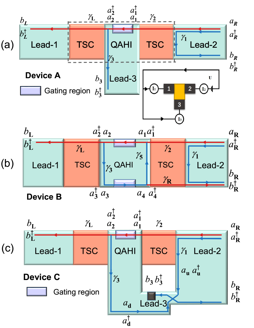
Figure 1: (color online) (a), (b) and (c) are schematic diagrams of three QAHI-TSC-QAHI-TSC-QAHI devices (Device A, Device B and Device C, respectively). In the schematic diagrams, the possible propagating routes of chiral Majorana fermions are shown, when an electron incomes from Lead-2. The lilac rectangle depicts the gating region. The red and green regions are the TSC and QAHI regions, respectively. The inset in (a) depicts the circuit layout for conductance measuring.

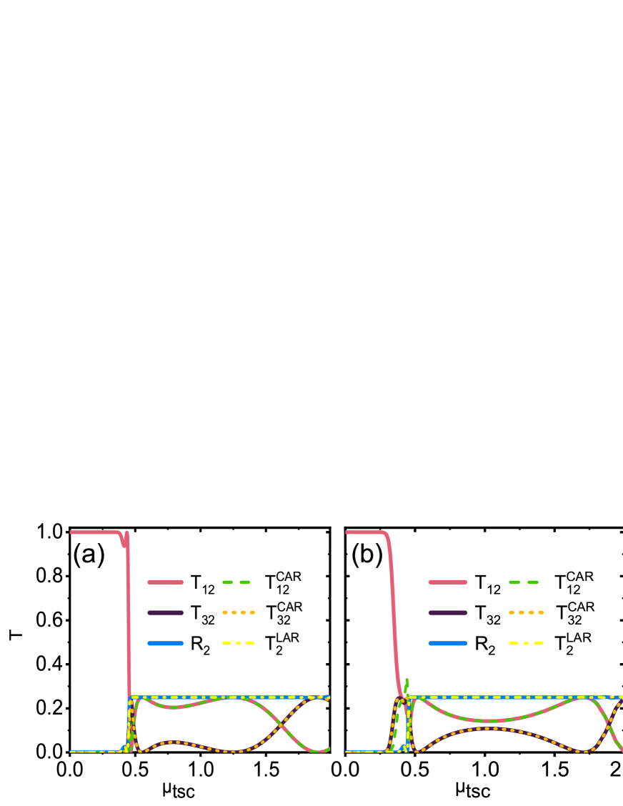
Figure 2: (color online) The transport properties of Device A. The normal transmission coefficients $T_{12}$ and $T_{32}$, the CAR coefficients $T^{\mathrm{CAR}}_{12}$ and $T^{\mathrm{CAR}}_{32}$, the normal reflection coefficient $R_{2}$, and the LAR coefficient $T^{\mathrm{LAR}}_{2}$ as functions of $\mu_{\mathrm{tsc}}$, with $\mu_{\mathrm{QAHI}}=0$ (a) and 0.2 (b), respectively. The gate voltage $V_{g}=0$, and the length of gating region $L_{v}=20a$. Here the normal transmission and reflection coefficients are plotted with solid lines, while CAR and LAR coefficients with dashed lines, so as to the distinction of outgoing electron or hole modes.

The scattering processes through two-terminal or three-terminal devices are analyzed by the nonequilibrium Green’s function techniqueDatta (1995), giving rise to the transmission coefficients as followsCheng et al. (2009),

$$T_{mn}(E) = \mathrm{Tr}[\Gamma^{m}_{ee}\textbf{G}^{r}_{ee}\Gamma^{n}_{ee}\textbf{G}^{a}_{ee}],$$ (4)

$$T^{\mathrm{CAR}}_{mn}(E) = \mathrm{Tr}[\Gamma^{m}_{ee}\textbf{ G}^{r}_{eh}\Gamma^{n}_{hh}\textbf{G}^{a}_{he}],$$ (5)

$$T^{\mathrm{LAR}}_{n}(E) = \mathrm{Tr}[\Gamma^{n}_{ee}\textbf{G}^{r}_{eh}\Gamma^{n}_{hh}\textbf{G}^{a}_{he}],$$ (6)

where $e$ and $h$ represent the electron and hole, respectively. $E$ denotes the incident energy. $n$ and $m$ are the indices of terminals, with $n\neq m$. $T_{mn}(E)$ and $T^{\mathrm{CAR}}_{mn}(E)$ are, respectively, the normal and CAR transmission coefficients from terminal $n$ to terminal $m$, and $T^{\mathrm{LAR}}_{n}(E)$ is the LAR coefficient at terminal $n$. ${\bf G}^{r}(E)=[E-\mathcal{H}_{\mathrm{cen}}-\sum_{n}{\bf\Sigma}^{r}_{n}]^{-1}$ is the retarded Green’s function, where $\mathcal{H}_{\mathrm{cen}}$ is the Hamiltonian of the central scattering region. The coupling between QAHI Lead-$n$ and the center region is described by the line-width function ${\Gamma}^{n}(E)=i[{\bf\Sigma}_{n}^{r}-{\bf\Sigma}_{n}^{a}]$, where the self-energy function satisfies ${\bf\Sigma}_{n}^{r}=[{\bf\Sigma}_{n}^{a}]^{\dagger}$. Since there is only one edge mode injecting from each QAHI terminal, the normal reflection coefficient at the QAHI terminal $n$ is

$$R_{n}=1-\!\sum\limits_{m(m\not=n)}\!T_{mn}\!-\!\sum\limits_{m}T^{\mathrm{CAR}}_{mn}-T^{\mathrm{LAR}}_{n}$$ (7)

III Results of Device A

In this section, we regulate the trajectory of chiral Majorana fermions by a designed Device A, based on the QAHI-TSC hybrid systems. Initially, we construct a QAHI-TSC-QAHI-TSC-QAHI device shown in Fig.1(a). The central scattering region, TSC-QAHI-TSC, is connected to three semi-infinite QAHI leads with widths $100a$, $100a$, and $60a$, respectively, labeled by Lead-1, Lead-2, and Lead-3. The length of two identical TSCs is $80a$. On the top of the centeral QAHI, an external gate voltage, $V_{g}$, is applied along the upper edge to tune the chemical potential. The gating region is colored lilac, of which the length, $L_{v}$, equals $20a$ unless specified otherwise. The width of the gating region, $W_{v}$, values $20a$, which is much longer than the broadening width of the chiral Dirac edge modes, ensuring that the Dirac edge carriers travel smoothly through this gating region. The energy of an incident electron from Lead-2 is fixed at $E=0$.

We discuss the transport process with the beginning of one electron mode from Lead-2, amount to two Majorana fermions. Trajectories of the injecting Majorana fermions are analyzed based on all the transmission coefficients and Andreev reflection coefficients through the three-terminal Device A, specifically labeled by $T_{12}$, $T_{32}$, $R_{2}$, $T^{\mathrm{CAR}}_{12}$, $T^{\mathrm{CAR}}_{32}$, and $T^{\mathrm{LAR}}_{2}$.

In order to illustrate the physical picture of the injecting Majorana fermions from Lead-2, we first study the transport without the gate voltage. Figure 2(a) shows the transmission coefficients and Andreev reflection coefficients versus the chemical potential of TSC, $\mu_{\mathrm{tsc}}$. From Fig.2(a), when $\mu_{\mathrm{tsc}}$ is less than a critical value $\mu_{\mathrm{tsc}}^{c}$, approximately 0.5 in our parameters, only the normal transmission coefficient from Lead-2 to Lead-1, $T_{12}$, is not zero with $T_{12}=1$, but $T_{32}=R_{2}=T^{\mathrm{CAR}}_{12}=T^{\mathrm{CAR}}_{32}=T^{\mathrm{LAR}}_{2}=0$. Because the TSC locates in the $\mathcal{N}=2$ TSC phase at $\mu_{\mathrm{tsc}}<\mu_{\mathrm{tsc}}^{c}$, which is topologically equivalent to the $\mathcal{C}=1$ QAHI. In this case, the carrier perfectly propagates via the chiral edge modes, counterclockwise from Lead-2 to Lead-1, from Lead-1 to Lead-3, and from Lead-3 to Lead-2. Given an incident electron from Lead-2, it would perfectly propagate to Lead-1 through the central TSC-QAHI-TSC region, as is the explanation for $T_{12}=1$, and $T_{32}=R_{2}=T^{\mathrm{CAR}}_{12}=T^{\mathrm{CAR}}_{32}=T^{\mathrm{LAR}}_{2}=0$ in Fig.3(a). On the other hand, once $\mu_{\mathrm{tsc}}$ exceeds the critical value $\mu_{\mathrm{tsc}}^{c}$, the TSC will jump into the $\mathcal{N}=1$ phase, and all the transmission coefficients and Andreev reflection coefficients appear with $T_{12}=T^{\mathrm{CAR}}_{12}$, $T_{32}=T^{\mathrm{CAR}}_{32}$, and $R_{2}=T^{\mathrm{LAR}}_{2}$ as shown in Fig.2(a). Here $R_{2}=T^{\mathrm{LAR}}_{2}=\frac{1}{4}$ is always true regardless of the chemical potential $\mu_{\mathrm{tsc}}$, but $T_{12}$, $T^{\mathrm{CAR}}_{12}$, $T_{32}$, and $T^{\mathrm{CAR}}_{32}$ depend on $\mu_{\mathrm{tsc}}$. This means that one of the two injecting Majorana fermions from Lead-2 is totally reflected back to Lead-2 and the other is transmitted to Lead-1 or Lead-3. Besides, when we adjust the chemical potential of QAHI, $\mu_{\mathrm{QAHI}}$, the results can well remain. For example, Fig.2(b) shows the six transmission coefficients at $\mu_{\mathrm{QAHI}}=0.2$. Here $T_{12}=1$ and $T_{32}=R_{2}=T^{\mathrm{CAR}}_{12}=T^{\mathrm{CAR}}_{32}=T^{\mathrm{LAR}}_{2}=0$ at $\mu_{\mathrm{tsc}}<\mu_{\mathrm{tsc}}^{c}$, and all the six transmission coefficients appear at $\mu_{\mathrm{tsc}}>\mu_{\mathrm{tsc}}^{c}$, which is very similar to that in Fig.2(a). Below, we concentrate on the $\mathcal{N}=1$ TSC phase to see the novel quantum oscillation.

Figure 3: (color online) $T_{12}$, $T_{32}$, $R_{2}$, $T^{\mathrm{CAR}}_{12}$, $T^{\mathrm{CAR}}_{32}$, and $T^{\mathrm{LAR}}_{2}$ versus the gate voltage $V_{g}$ for the different chemical potentials of TSC, $\mu_{\mathrm{tsc}}=0.2,\ 0.55,\ 1,\ 2$ for (a), (b), (c), and (d) respectively. All the unmentioned parameters are the same as Fig.2(a).

Figure 3 shows the normal transmission coefficients and Andreev reflection coefficients versus the gate voltage $V_{g}$ at several specific chemical potentials $\mu_{\mathrm{tsc}}$. When $\mu_{\mathrm{tsc}}=0.2<\mu_{\mathrm{tsc}}^{c}$, the normal transmission coefficient $T_{12}=1$ exactly and $T_{32}=R_{2}=T^{\mathrm{CAR}}_{12}=T^{\mathrm{CAR}}_{32}=T^{\mathrm{LAR}}_{2}=0$ [see Fig.3(a)], because the TSC locates in the $\mathcal{N}=2$ TSC phase. On the other hand, when the TSC is in the $\mathcal{N}=1$ TSC phase with $\mu_{\mathrm{tsc}}>\mu_{\mathrm{tsc}}^{c}$ in Figs.3(b-d), the normal reflection and the LAR coefficients $R_{2}=T^{\mathrm{LAR}}_{2}=\frac{1}{4}$. In particular, the normal transmission coefficients ($T_{12}$ and $T_{32}$) and the CAR coefficients ($T^{\mathrm{CAR}}_{12}$ and $T^{\mathrm{CAR}}_{32}$) oscillate with the gate voltage $V_{g}$. The oscillations always maintain themselves as long as $\mu_{\mathrm{tsc}}>\mu_{\mathrm{tsc}}^{c}$ [see Figs.3(b-d)]. The amplitude of the oscillation is $1/4$. When $T_{12}$ and $T^{\mathrm{CAR}}_{12}$ oscillate to the maximum $1/4$, $T_{32}$ and $T^{\mathrm{CAR}}_{32}$ oscillate to the minimum $0$, and vice versa. In addition, $T_{12}=T^{\mathrm{CAR}}_{12}$, $T_{32}=T^{\mathrm{CAR}}_{32}$, and $T^{\mathrm{CAR}}_{12}+T^{\mathrm{CAR}}_{32}=1/4$.

Let us analyze the trajectory of chiral Majorana fermions, discuss the control of their propagating route, and explain results in Fig.3 when TSC is in the $\mathcal{N}=1$ phase. To begin with, a Dirac electron injects from Lead-2, which is tantamount to two Majorana fermions, $a_{R}=\frac{\sqrt{2}}{2}(\gamma_{1}+i\gamma_{2})$. At the boundary of Lead-2 and the right TSC, one of the Majorana fermions $\gamma_{1}$ is totally reflected, travels down and backscatters to Lead-2. Thus, the outgoing electron and hole modes appear equiprobably, $\gamma_{1}=\frac{\sqrt{2}}{2}(b_{R}+b^{{\dagger}}_{R})$, and we can obtain the normal reflection and LAR coefficients,

$$R_{2}=T^{\mathrm{LAR}}_{2}=1/4.$$ (8)

On the other hand, the other Majorana fermion $\gamma_{2}$ passes through the right TSC and reaches the central QAHI region as mixing of electron and hole, $\gamma_{2}=\frac{\sqrt{2}}{2i}(a_{1}-a^{{\dagger}}_{1})$, as shown in Fig.1(a). Then passing the central gating region, the electron mode $a_{1}$ can acquire a dynamical phase $\phi$ and become $a_{2}$. At the same time, the hole mode $a^{{\dagger}}_{1}$ gains an opposite phase $-\phi$ and thus becomes $a^{{\dagger}}_{2}$,

$$a_{2}=e^{i\phi}a_{1},\ a^{{\dagger}}_{2}=e^{-i\phi}a^{{\dagger}}_{1},$$ (9)

where $\phi$ is the dynamical phase controlled by the gate voltage $V_{g}$. Then, again at the QAHI-left TSC boundary, splitting happens: one Majorana fermion $\gamma_{L}$ is transmitted to Lead-1, $\gamma_{L}=\frac{\sqrt{2}}{2i}(a_{2}-a^{{\dagger}}_{2})$, while the other Majorana fermion $\gamma_{3}$ is reflected to Lead-3, $\gamma_{3}=\frac{\sqrt{2}}{2}(a_{2}+a^{{\dagger}}_{2})$. The outgoing Majorana modes have the relations to the original Majorana mode $\gamma_{2}$ as,

$$\gamma_{L}=\gamma_{2}\sin\phi,\ \gamma_{3}=\gamma_{2}\cos\phi.$$ (10)

When $\phi=0$, $\gamma_{3}=\gamma_{2}$, the Majorana state $\gamma_{2}$ totally ejects into Lead-3, but when $\phi=\frac{\pi}{2}$, $\gamma_{L}=\gamma_{2}$, which means $\gamma_{2}$ entirely departs via Lead-1. With other values of the phase $\phi$, the incoming Majorana fermion $\gamma_{2}$ is controlled to leave partially through Lead-1 and Lead-3. So we can well control the propagating route of the chiral Majorana fermion by tuning the phase $\phi$. Eventually, the Majorana fermions $\gamma_{L}$ and $\gamma_{3}$ respectively eject into Lead-2 and Lead-3, leading that the normal transmission coefficients and CAR coefficients are,

$$T_{12}=T^{\mathrm{CAR}}_{12}=(1/4){\sin}^{2}(\phi+\phi_{0}),$$ (11)

$$T_{32}=T^{\mathrm{CAR}}_{32}=(1/4){\cos}^{2}(\phi+\phi_{0}),$$ (12)

and $T_{12}+T_{32}=T^{\mathrm{CAR}}_{12}+T^{\mathrm{CAR}}_{32}=1/4$, where $\phi_{0}$ denotes the initial phase. The sinusoidal oscillations of the normal transmission coefficients and CAR coefficients are well consistent with the numerical curves in Figs.3(b-d). Notice that here the normal transmission coefficient $T_{12}$ ($T_{32}$) is always equal to the CAR coefficient $T^{\mathrm{CAR}}_{12}$ ($T^{\mathrm{CAR}}_{32}$), because the outgoing Majorana fermion $\gamma_{L}$ ($\gamma_{3}$) to Lead-1 (Lead-3) has the same components of electron and hole. It is worth to mention that if the right TSC is removed, the single QAHI-TSC-QAHI device can no longer control the chiral Majorana fermion to Lead-1 and Lead-3 by tuning the gate voltage, stemming from the coexistence of $\gamma_{1}$ and $\gamma_{2}$ in the right QAHI. Remarkably, the two-TSC structure with $\mathcal{N}=1$ in Device A is essential to control chiral Majorana fermions into different terminals via electrical gating.

Then let us explain how the gate voltage modulates trajectories of Majorana modes continuously. When a gate voltage $V_{g}$ is applied to the upper edge of the central QAHI region, it directly adjusts the Fermi level of QAHI, and thus the momenta $k$ of electrons and holes with energy $E=0$ are changed. By varying the gate voltage, the obtained dynamical phase $\phi$, explicit to be ${kL_{v}}$ with $L_{v}$ the length of the gating region, can tune the probabilities that the incoming Majorana mode $\gamma_{2}$ chooses to go to Lead-1 or Lead-3, as Eq.(10). Under a fixed length $L_{v}$, the normal tunneling coefficients $T_{12}$ and $T_{32}$ sinusoidally oscillate in the same period, in response to a continuously varying $V_{g}$, as depicted in Figs.3(b-d).

If the TSC locates in the $\mathcal{N}=1$ TSC phase with $\mu_{\mathrm{tsc}}>\mu_{\mathrm{tsc}}^{c}$, the chemical potential $\mu_{\mathrm{tsc}}$ of TSC has no influence on the period and amplitude of the transmission oscillation. From Figs.3(b-d), we can see that the oscillation amplitudes are always $1/4$ regardless of $\mu_{\mathrm{tsc}}$. Here the chemical potential $\mu_{\mathrm{tsc}}$ merely changes the initial phase $\phi_{0}$ of the oscillation of transmission coefficients versus $V_{g}$, by comparing Figs.3(b), (c), and (d). This phase shift originates from the fact that a Dirac wave function requires a matching condition with the Majorana wave functions at the left TSC-central QAHI boundary due to the transverse broadening of wave functions.

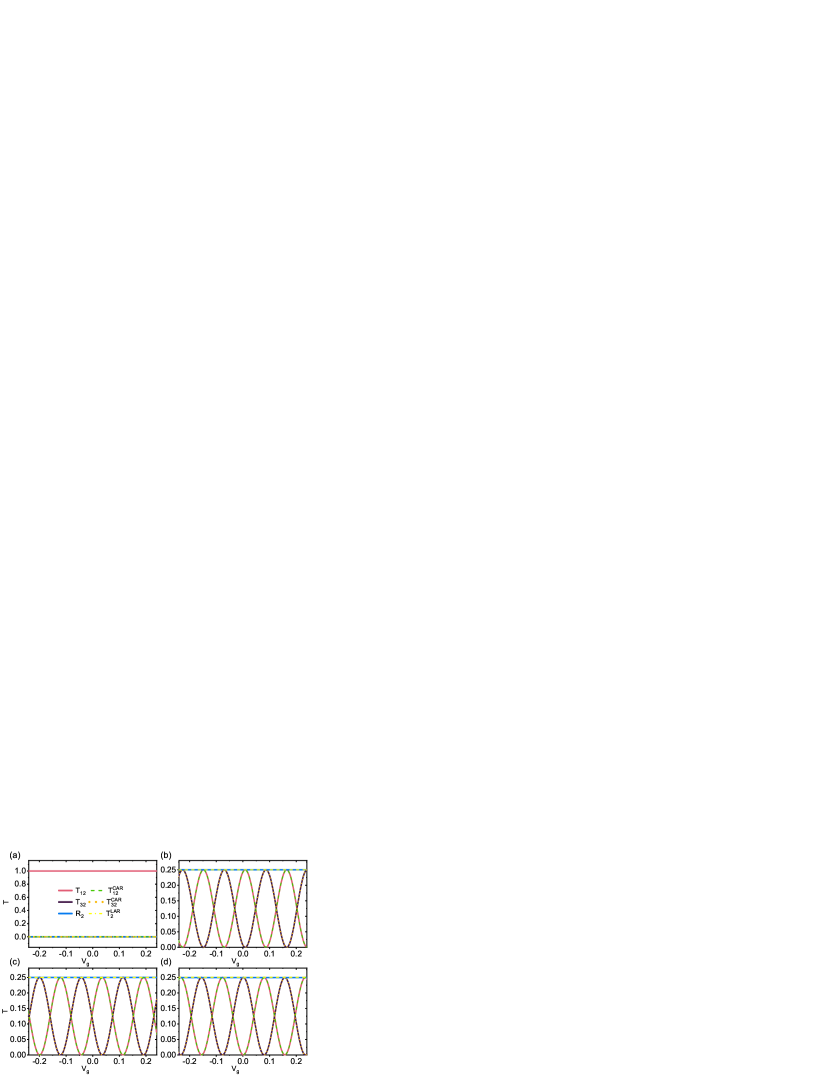
Figure 4: (color online) $T_{12}$, $T_{32}$, $R_{2}$, $T^{\mathrm{CAR}}_{12}$, $T^{\mathrm{CAR}}_{32}$, and $T^{\mathrm{LAR}}_{2}$ versus the gate voltage $V_{g}$ for the different chemical potentials of TSC, $\mu_{\mathrm{tsc}}=0.2,\ 0.55,\ 1,\ 2$ for (a), (b), (c), and (d) respectively. All the unmentioned parameters are the same as Fig.2(b).

The chemical potential $\mu_{\mathrm{QAHI}}$ of the QAHI region does not affect on the oscillating behavior of the transmission coefficients, but just arouses a horizonal shift compared to the initial curves. By increasing $\mu_{\mathrm{QAHI}}$ from 0 to 0.2, we plot transmission coefficients in Fig.4 as a comparison for Fig.3. In Fig.4(a) $\mu_{\mathrm{tsc}}=0.2<\mu_{\mathrm{tsc}}^{c}$, the TSC is at the $\mathcal{N}=2$ TSC phase, here only $T_{12}=1$ and other transmission and Andreev reflection coefficients are zero, as is in complete agreement with Fig.3(a). In this case, two Majorana fermions are totally transmitted from Lead-2 into Lead-1 without reflection. As the chemical potential $\mu_{\mathrm{tsc}}$ increases, different topological properties between the QAHI and $\mathcal{N}=1$ TSC appear so that Device A can regulate the Majorana mode via electrical gating as before. Now the transmission coefficients ($T_{12}$ and $T_{32}$) and the CAR coefficients ($T^{\mathrm{CAR}}_{12}$ and $T^{\mathrm{CAR}}_{32}$) oscillate with the gate voltage $V_{g}$, which is consistent with that in Figs.3(b-d). However, due to the increase of the chemical potential $\mu_{\mathrm{QAHI}}$, the momenta $k$ of zero-energy electrons and holes through the gating QAHI region are no longer zero when $V_{g}=0$. It behaves like an additional phase $e^{i\phi_{\mathrm{QAHI}}}$ to $a_{1}$, and $e^{-i\phi_{\mathrm{QAHI}}}$ to $a^{\dagger}_{1}$. So the transmission and Andreev reflection coefficients are,

$$R = T^{\mathrm{LAR}}=1/4,$$ (13)

$$T_{12} = T^{\mathrm{CAR}}_{12}=(1/4){\sin}^{2}(\phi+\phi_{0}+\phi_{\mathrm{QAHI}}),$$ (14)

$$T_{32} = T^{\mathrm{CAR}}_{32}=(1/4){\cos}^{2}(\phi+\phi_{0}+\phi_{\mathrm{QAHI}}).$$ (15)

Or rather to say, the non-zero $\mu_{\mathrm{QAHI}}$ can be regarded as an initial gating voltage, and thus it does not influence the period and amplitude of any transmission oscillation. The phase shift can be clearly seen by comparing Figs.4(b-d) with Figs.3(b-d), respectively.

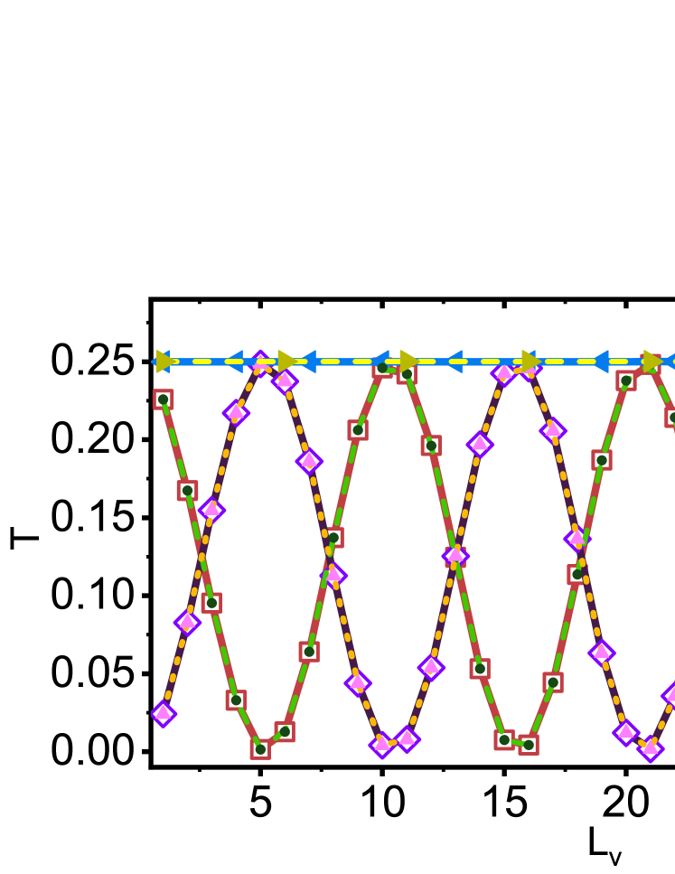
Figure 5: (color online) $T_{12}$, $T_{32}$, $R_{2}$, $T^{\mathrm{CAR}}_{12}$, $T^{\mathrm{CAR}}_{32}$, and $T^{\mathrm{LAR}}_{2}$ as functions of the length of gating region $L_{v}$, where $\mu_{\mathrm{QAHI}}=0$, $\mu_{\mathrm{tsc}}=0.55$, and $V_{g}=0$. All the unmentioned parameters are the same as Fig.2(a).

In Fig.5, we plot the transmission coefficients as a function of the length $L_{v}$ of the gating region in the central QAHI, and find that $R_{2}$ and $T^{\mathrm{LAR}}_{2}$ keep a constant $1/4$ and the transmission coefficients behave periodically oscillating versus the length $L_{v}$ because of the dynamical phase $\phi=kL_{v}$. In addition, we change the length of the gating region, and find that oscillations of transmission coefficients in Figs.3 and 4 always exist. It is the length $L_{v}$ that determines the period of the oscillation. Since the dynamical phase has an explicit form, $e^{ikL_{v}}$, the identical oscillating period in Figs.3 and 4 is relevant to $\frac{2\pi}{L_{v}}$. The longer $L_{v}$ is, the faster the oscillation becomes versus the gate voltage $V_{g}$.

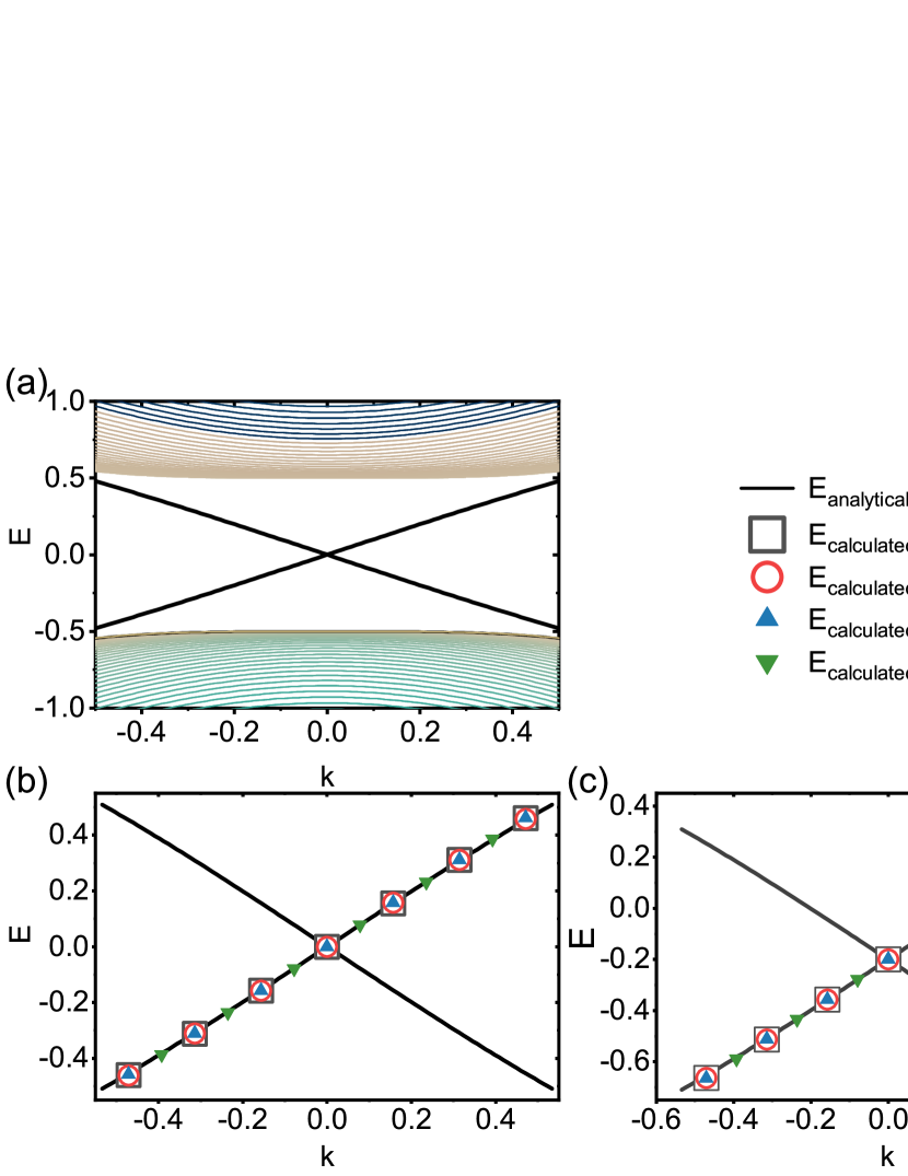
Figure 6: (color online) (a) Band structure of the QAHI nanoribbon with the width of $100a$ and $\mu_{\mathrm{QAHI}}=0$. Black lines are bolded for the edge states of QAHI. (b) and (c) are the energy dispersions obtained from the transmission coefficients in Figs.3(b-d) and Figs.4(b-d), with $\mu_{\mathrm{QAHI}}=0$ and $\mu_{\mathrm{QAHI}}=0.2$, respectively. The black solid lines in (b) and (c) are the analytical edge states directly from (a) for comparison. All the unmentioned parameters are the same as Fig.2.

Furthermore, the energy dispersion of the chiral Dirac edge states of the central QAHI could be obtained according to the periodic oscillation of transmission coefficients versus the gate voltage. From the Hamiltonian of QAHI with $\mu_{\mathrm{QAHI}}=0$ in Eq.(2), we can directly calculate the energy dispersion by considering a QAHI nanoribbon, as shown in Fig.6(a). Two chiral Dirac edge states, bolded in Fig.6(a), traverse across the bulk band gap, exactly at $E=0$ and $k=0$. From the periodic oscillation of transmission coefficients in Fig.3, we can obtain the energy dispersion of edge states. While the chemical potential $\mu_{\mathrm{QAHI}}=0$ and the gate voltage $V_{g}=0$, the momentum $k$ is set to zero. With a given gating length $L_{v}$, after $n$ periodic oscillations (with the integer $n=0,\ \pm 1,\ \pm 2$, …), the momentum is $k_{n}=n\pi/L_{v}$ originating from the period of $T_{12}=(1/4){\sin}^{2}(kL_{v})$, and the corresponding energy $E_{n}$ can be obtained from the periodic oscillation curves in Fig.3, with $E_{n}=V_{gn}$ where $V_{gn}$ is the value of the gate voltage after $n$ periodic oscillations. Based on the data $(E_{n},\ k_{n})$, we can plot a series of discrete points in Fig.6(b). For comparison, the analytical energy dispersion of edge states from Fig.6(a) is also displayed in Fig.6(b). The dispersion relation obtained from transmission coefficients conforms perfectly to the analytical black curve. This provides an effective method to measure the energy dispersion relation of the chiral Dirac edge state experimentally. Notably, this measuring method is free from different TSC’s chemical potential $\mu_{\mathrm{tsc}}$, shown in Fig.6(b) where all the markers obtained from the different $\mu_{\mathrm{tsc}}$ locate on the same analytical curve. Considering the initial chemical potential $\mu_{\mathrm{QAHI}}$ of QAHI, the varying $\mu_{\mathrm{QAHI}}$ just moves down the Fermi level and changes the momenta of Dirac fermions in the gating region but has no effects on the structure of the dispersion relation, so the calculated $E-k$ relation of $\mu_{\mathrm{QAHI}}=0.2$ could also be obtained only with a shift along $E$ axis in Fig.6(c), and the discrete data points are obtained from Figs.4(b-d).

Finally, we calculate the conductance of Device A. Using the multi-probe Landauer-Büttiker formula, the current in Lead-$n$ at the small bias limit can be calculated,Sun et al. (1999); Sun and Xie (2009)

$$I_{n} = \frac{e^{2}}{h}\left[\sum_{m(m\not=n)}(V_{n}-V_{m})T_{mn}\right.$$ (16)

$$\left.+2V_{n}T^{\mathrm{LAR}}_{n}+\sum_{m(m\not=n)}(V_{n}+V_{m})T^{\mathrm{CAR}}_{mn}\right]$$

$$= \!\frac{e^{2}}{h}\!\left[\!V_{n}(1\!+\!T_{n}^{\mathrm{L\!A\!R}}\!-\!R_{n})\!+\!\sum_{m(\!m\!\not=\!n\!)}\!V_{m}(T_{\!m\!n}^{\mathrm{C\!A\!R}}\!-\!T_{\!m\!n})\!\right]\!,$$

where $V_{n}$ is the voltage of Lead-$n$, and voltages of superconductors are set to zero. Based on the circuit in the inset of Fig.1(a) to measure the three-terminal conductance of Device A, the linear conductances $G_{n}$ ($G_{n}\equiv I_{n}/V_{n}$ with $n=1,2,3$) at all three leads are constant with $G_{1}=G_{2}=G_{3}=\frac{e^{2}}{h}$, and $G_{n}$ does not oscillate with the gate voltage, when the TSC is in the $\mathcal{N}=1$ TSC phase. In fact, regardless of the connection of the external circuit, the conductance $G_{n}$ of Device A is always constant, although the normal transmission and Andreev reflection coefficients oscillate with the gate voltage. In the $\mathcal{N}=1$ TSC phase, the two injecting chiral Majorana fermions from Lead-$n$ respectively transmit into Lead-2, Lead-1, and Lead-3, so that the outgoing electron and hole in all three leads are equiprobable, leading to the relations of the transmission coefficients and Andreev reflection coefficients:

$$T_{mn}=T^{\mathrm{CAR}}_{mn},\hskip 5.69054pt R_{n}=T^{\mathrm{LAR}}_{n},$$ (17)

as shown in Figs.3(b-d) and Figs.4(b-d). Thus, $I_{n}=(e^{2}/h)V_{n}$ from Eq.(16), and Device A gives no contribution to the observable oscillation of the conductance versus the gate voltage. Motivated by the desire for an experimentally observable oscillation of physical quantity, we proceed with the analysis of Devices B and C in the following sections.

IV Results of Device B

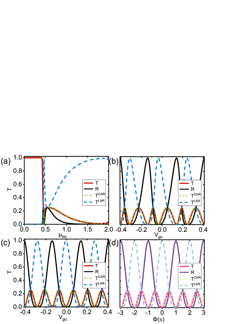
Figure 7: (color online) The transport properties of Device B. (a) The normal tunneling coefficients $T$, the CAR coefficients $T^{\mathrm{CAR}}$, the normal reflection coefficient $R$, and the LAR coefficient $T^{\mathrm{LAR}}$ as functions of the chemical potential $\mu_{\mathrm{tsc}}$ of the TSC, with $\mu_{\mathrm{QAHI}}=0$, $L_{v}=20a$, $V_{gu}=V_{gl}=0$. (b) and (c) are the transmission coefficients versus the upper gating voltage $V_{gu}$ with $\mu_{\mathrm{tsc}}=1.5$ and $1.8$, respectively. All the unmentioned parameters are the same as in (a). (d) The analytical transmission coefficients versus the dynamical phase $\phi$ derive from the Eqs.(23-25), setting $\phi_{u}=\phi+\frac{\pi}{2}$ and $\phi_{l}=\frac{\pi}{2}$, fitting with curves in Fig.7(c)

For the purpose of observing the manipulation of the chiral Majorana fermions in the experiments, in this section, we design a two-terminal QAHI-TSC-QAHI-TSC-QAHI Device B as shown in Fig.1(b). Below, we study the transport properties of chiral Majorana fermions both analytically and numerically, and then successfully obtain the observable conductance oscillation as well as the successive energy dispersion of the chiral Dirac edge modes. In Device B, an additional lower gate in the central QAHI region is added, and it plays the same role as the upper gate [see Fig.1(b)]. More importantly, it is a cyclic trajectory of the chiral Majorana edge mode locating in the central QAHI region that causes the conductance oscillation.

Similarly, for Device B, the normal transmission coefficient $T$, the normal reflection coefficient $R$ and the CAR and LAR coefficients ($T^{\mathrm{CAR}}$ and $T^{\mathrm{LAR}}$) can be calculated from Eqs.(4-7). Fig.7(a) shows $T$, $R$, $T^{\mathrm{CAR}}$, and $T^{\mathrm{LAR}}$ as functions of the chemical potential $\mu_{\mathrm{tsc}}$ of the TSC region. When $\mu_{\mathrm{tsc}}<\mu_{\mathrm{tsc}}^{c}$, the TSC is in the $\mathcal{N}=2$ TSC phase, with the normal transmission coefficient $T=1$ and $T^{\mathrm{CAR}}=R=T^{\mathrm{LAR}}=0$. These stable coefficients occur because the injecting Dirac electron from the right QAHI, which is equivalent to two injecting chiral Majorana fermions, passes through the center TSC-QAHI-TSC region and directly ejects from the left QAHI. However, when the chemical potential $\mu_{\mathrm{tsc}}>\mu_{\mathrm{tsc}}^{c}$, the TSC is in the $\mathcal{N}=1$ TSC phase. Thus, the reflection of chiral Majorana fermions occurs at the interface of the QAHI and TSC, resulting in the transport process where transmission coefficients $T$, $R$, $T^{\mathrm{CAR}}$, and $T^{\mathrm{LAR}}$ are usually non-zero. From hereon, we focus on the $\mathcal{N}=1$ TSC phase with $\mu_{\mathrm{tsc}}>\mu_{\mathrm{tsc}}^{c}$. Figs.7(b and c) show the transmission coefficients versus the upper gate voltage $V_{gu}$ for the fixed chemical potential $\mu_{\mathrm{tsc}}=1.5$ and $1.8$, respectively. All of the four transmission coefficients ($T$, $R$, $T^{\mathrm{CAR}}$, and $T^{\mathrm{LAR}}$) oscillate with the gate voltage $V_{gu}$. The oscillation amplitude of the normal reflection and LAR coefficients is about 1 but that of the normal transmission and CAR coefficients is about 1/4. The oscillation period of $R$ and $T^{\mathrm{LAR}}$ is twice longer than that of $T$ and $T^{\mathrm{CAR}}$. In addition, $T=T^{\mathrm{CAR}}$ always keeps, but $R$ is not equal to $T^{\mathrm{LAR}}$ as usual. The oscillation of transmission coefficients versus $V_{gu}$ can well remain regardless of the chemical potentials ($\mu_{\mathrm{tsc}}$, $\mu_{\mathrm{QAHI}}$) and the lower gate voltage $V_{gl}$, as long as the TSC is in the $\mathcal{N}=1$ TSC phase. Different from Device A, the chemical potential $\mu_{\mathrm{tsc}}$ does not only shift the initial phase of transmission curves but also obviously changes the shape of curves [see Figs.7(b and c)].

Let us analyze the propagating route of chiral Majorana fermions and give the analytical expressions of the normal transmission and Andreev reflection coefficients of Device B in the $\mathcal{N}=1$ TSC phase. Considering that an electron $a_{R}$ from Lead-2 propagates along the upper side of QAHI, also regarded as two chiral Majorana fermions $\gamma_{1}$ and $\gamma_{2}$ with $\gamma_{1}=\frac{\sqrt{2}}{2}(a_{R}+a_{R}^{\dagger})$ and $\gamma_{2}=\frac{\sqrt{2}}{2i}(a_{R}-a_{R}^{\dagger})$. When they reach the right QAHI-TSC interface, $\gamma_{2}$ passes through the right TSC while $\gamma_{1}$ is reflected back to the right QAHI, i.e., Lead-2 [see Fig.1(b)]. Then $\gamma_{2}$ leaves along the edge of the right TSC and enters into the central QAHI with upper and lower gates. To avoid confusion, let us label the four electron modes at the vertices of the central QAHI region as $a_{1}$, $a_{2}$, $a_{3}$, and $a_{4}$, from the upper right to the lower right in the counterclockwise direction, and similarly the hole modes as $a^{{\dagger}}_{1}$, $a^{{\dagger}}_{2}$, $a^{{\dagger}}_{3}$, and $a^{{\dagger}}_{4}$. The initially incoming electron $a_{1}$ can travel along the upper gating QAHI edge and get a dynamical phase $\phi_{u}$, while the hole $a^{{\dagger}}_{1}$ acquires the phase $-\phi_{u}$, that is,

$$a_{2}=e^{i\phi_{u}}a_{1},\ a^{{\dagger}}_{2}=e^{-i\phi_{u}}a^{{\dagger}}_{1}.$$ (18)

The combination of $a_{2}$ and $a^{{\dagger}}_{2}$ splits two chiral Majorana fermions $\gamma_{L}=\frac{\sqrt{2}}{2i}(a_{2}-a^{{\dagger}}_{2})$ and $\gamma_{3}=\frac{\sqrt{2}}{2}(a_{2}+a^{{\dagger}}_{2})$. $\gamma_{L}$ directly goes through the left TSC into Lead-1 with $b_{L}=\frac{i\sqrt{2}}{2}\gamma_{L}$ and $b^{{\dagger}}_{L}=\frac{-i\sqrt{2}}{2}\gamma_{L}$, while the other Majorana fermion $\gamma_{3}$ moves down counterclockwise. Also, at the lower left vertex of the central QAHI, $\gamma_{3}$ could be seen as the combination of the electron mode $a_{3}$ and the hole mode $a^{{\dagger}}_{3}$ with $a_{3}=\frac{\sqrt{2}}{2}\gamma_{3}$ and $a^{{\dagger}}_{3}=\frac{\sqrt{2}}{2}\gamma_{3}$, which acquire opposite phases $\phi_{l}$ and $-\phi_{l}$, respectively, when passing along the lower QAHI edge,

$$a_{4}=e^{i\phi_{l}}a_{3},\ a^{{\dagger}}_{4}=e^{-i\phi_{l}}a^{{\dagger}}_{3}.$$ (19)

Afterward, the gated modes $a_{4}$ and $a^{{\dagger}}_{4}$ can again be seen as two Majorana modes, $a_{4}=\frac{\sqrt{2}}{2}(\gamma_{5}+i\gamma_{R})$. $\gamma_{5}$ is reflected back to $a_{1}$, while $\gamma_{R}$ ejects out and eventually combines with $\gamma_{1}$ to produce the outgoing modes of Lead-2 as $b_{R}=\frac{\sqrt{2}}{2}(\gamma_{1}+i\gamma_{R})$ and $b^{{\dagger}}_{R}=\frac{\sqrt{2}}{2}(\gamma_{1}-i\gamma_{R})$. Notice that the chiral Dirac electron $a_{1}$ and the hole $a_{1}^{\dagger}$ at the upper right vertex of the central QAHI originate from the Majorana fermions $\gamma_{2}$ and $\gamma_{5}$,

$$a_{1}=(\sqrt{2}/2)(\gamma_{5}+i\gamma_{2}),\ a^{{\dagger}}_{1}=(\sqrt{2}/2)(\gamma_{5}-i\gamma_{2}).$$ (20)

Then we combine equations all above [from Eq.(18) to Eq.(20)], adopt the scattering matrix method, and express the outgoing modes ($b_{L},b_{L}^{\dagger},b_{R},b_{R}^{\dagger}$) by the incoming modes ($a_{R},a_{R}^{\dagger}$) as follows:

$$\left(\begin{array}[]{cc}b_{L}\\ b^{{\dagger}}_{L}\\ \end{array}\right)=\frac{1}{2}X\left(\begin{array}[]{cc}1&-1\\ -1&1\\ \end{array}\right)\left(\begin{array}[]{cc}a_{R}\\ a^{{\dagger}}_{R}\\ \end{array}\right),$$ (21)

$$\left(\begin{array}[]{cc}b_{R}\\ b^{{\dagger}}_{R}\\ \end{array}\right)=\frac{1}{2}\left(\begin{array}[]{cc}1+Y&1-Y\\ 1-Y&1+Y\\ \end{array}\right)\left(\begin{array}[]{cc}a_{R}\\ a^{{\dagger}}_{R}\\ \end{array}\right),$$ (22)

where $X$ and $Y$ are coefficients related to the dynamical phases, $X=\frac{\cos(\phi_{u})-\cos(2\phi_{u})\cos(\phi_{l})}{1-\cos(\phi_{u})\cos(\phi_{l})}$ and $Y=\frac{\sin(\phi_{u})\sin(\phi_{l})}{1-\cos(\phi_{u})\cos(\phi_{l})}$. Finally, the transmission and Andreev reflection coefficients of Device B are analytically obtained,

$$\displaystyle T = T^{\mathrm{CAR}}=(1/4)X^{2},$$ (23)

$$\displaystyle R = (1/4)(1+Y)^{2},$$ (24)

$$\displaystyle T^{\mathrm{LAR}} = (1/4)(1-Y)^{2}.$$ (25)

Here the normal transmission coefficient $T$ is always the same as the CAR coefficient $T^{\mathrm{CAR}}$, which is well consistent with numerical results in Figs.7(b and c), because the outgoing electron $b_{L}$ and the hole $b^{\dagger}_{L}$ share the same Majorana mode $\gamma_{L}$. However, the reflective mode, $b_{R}$, is a mixture of two Majorana modes, $\gamma_{1}$ and $\gamma_{R}$ [see Fig.1(b)]. Thus, it is no wonder that the probability of an outgoing electron differs from that of a hole in Lead-2, as is why the normal reflection coefficients $R$ is usually not equal to the LAR coefficients $T^{\mathrm{LAR}}$ plotted in Figs.7(b and c). From Eq.(16), this difference will eventually give rise to an oscillating conductance to be shown later. Furthermore, since there is only a Majorana fermion $\gamma_{L}$ outgoing to Lead-1, the normal transmission and CAR coefficients are always less than $1/4$, but the normal reflection and LAR coefficients can exceed $1/4$ due to two Majorana fermions $\gamma_{R}$ and $\gamma_{1}$ outgoing to Lead-2.

By setting $\phi_{u}=\phi+\frac{\pi}{2}$ and $\phi_{l}=\frac{\pi}{2}$, the analytical transmission coefficients are plotted in Fig.7(d). Here, analytical results accommodate well with numerical calculations in Fig.7(c). Definitely, trajectories of Majorana fermions are regulated by changing the dynamical phase $\phi$ which can be tuned by the upper or lower gate of the central QAHI. Let us discuss the control of the propagating route of Majorana fermion $\gamma_{2}$ that always passes through the right TSC into the central QAHI. When $\phi=\pi$, $R=1$ and $T=T^{\mathrm{CAR}}=T^{\mathrm{LAR}}=0$, namely, the Majorana fermion $\gamma_{2}$ is reflected at the left TSC-central QAHI interface with $\gamma_{L}=0$ and $\gamma_{R}=\gamma_{2}$. But at $\phi=\pi/2$, $R=T=T^{\mathrm{CAR}}=T^{\mathrm{LAR}}=1/4$, namely, $\gamma_{2}$ totally ejects through the left TSC into Lead-1 with $\gamma_{L}=\gamma_{2}$ and $\gamma_{R}=0$. When $\phi=0$, $T^{\mathrm{LAR}}=1$, while $T=T^{\mathrm{CAR}}=R=0$, that is, $\gamma_{2}$ gets a phase $\pi$ and is totally reflected with $\gamma_{L}=0$ and $\gamma_{R}=e^{i\pi}\gamma_{2}$. With other values of phase $\phi$, the incoming Majorana fermion $\gamma_{2}$ is controlled to leave partially into Lead-1 and to be reflected back partially. Thus, by tuning the gate voltage, we do control the trajectory of chiral Majorana fermions.

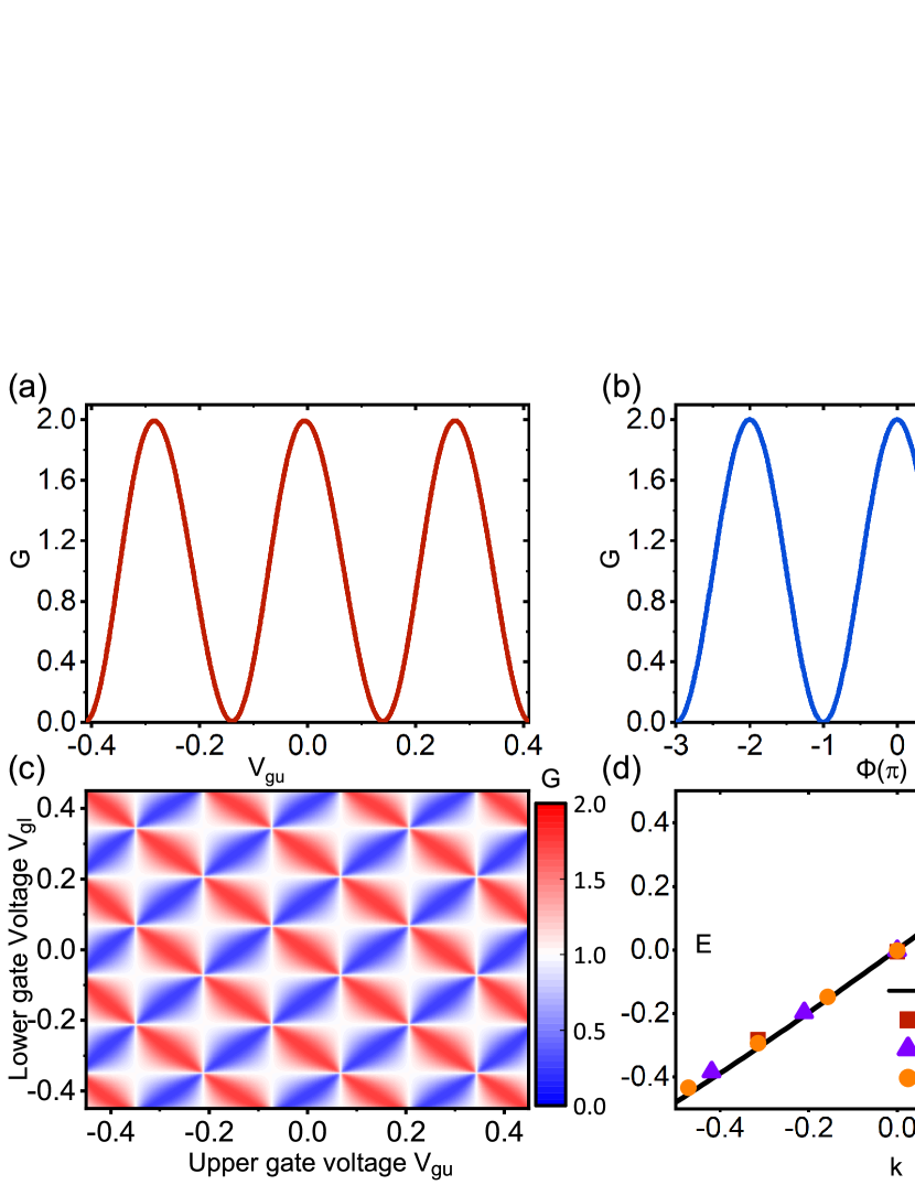
Figure 8: (color online) (a) and (b) are the linear conductance $G$ of Device B as a function of the upper gate voltage $V_{gu}$ and the dynamical phase $\phi$ from the numerical calculations and analytical results, respectively. (c) Colormap of conductance $G$ as a function of both the upper gate voltage $V_{gu}$ and lower gate voltage $V_{gl}$. (d) The numerical calculated energy dispersions from the oscillating conductance. Differently colored markers correspond to different length $L_{v}$ of the gate region. The black solid lines are the analytical energy dispersion relation from Fig.6(a). All the unmentioned parameters are the same as Figs.7(c and d).

Then we calculate the linear conductance $G$ of Device B, which is derived from Eq.(16) as,

$$G=\frac{dI}{dU}=\frac{e^{2}}{h}(T+T^{\mathrm{CAR}}+2T^{\mathrm{LAR}}),$$ (26)

where $U=V_{2}-V_{1}$ is the bias voltage between Lead-2 and Lead-1. Combined with the relation in Eq.(7), the linear conductance can be written in a plain form, $G=\frac{e^{2}}{h}(1+T^{\mathrm{LAR}}-R)$. Fig.8(a) shows the conductance $G$ versus the upper gate voltage $V_{gu}$, where $G$ periodically oscillates with the gate voltage $V_{gu}$ with the oscillation amplitude being $\frac{2e^{2}}{h}$. In fact, although the normal transmission coefficient $T$ is always accordant with the CAR coefficient $T^{\mathrm{CAR}}$, the normal reflection coefficient $R$ and the LAR coefficient $T^{\mathrm{LAR}}$ usually separate from each other [see Figs.7(b and c)], so the conductance $G$ can take on a significant oscillation in Fig.8(a).

By using Eqs.(23-25), the analytical expression of $G$ is explicitly denoted as

$$G=\frac{e^{2}}{h}\left(1+\frac{\sin(\phi_{u})\sin(\phi_{l})}{1-\cos(\phi_{u})\cos(\phi_{l})}\right)$$ (27)

When setting $\phi_{u}=\phi+\frac{\pi}{2}$ and $\phi_{l}=\frac{\pi}{2}$, we plot the analytical conductance $G$ corresponding to the dynamical phase $\phi$ in Fig.8(b), which is completely consistent with the numerical curve in Fig.8(a).

Fig.8(c) shows the colormap of conductance $G$ as a function of upper and lower gate voltages, $V_{gu}$ and $V_{gl}$. The conductance periodically oscillates with both $V_{gu}$ and $V_{gl}$, and it presents the equivalent effects of tuning the upper and the lower gate voltages. Also, the conductance undulation appears a shuttle-like pattern in each period. As shown by now, the oscillating conductance is experimentally observable. Meanwhile, this quantum oscillation phenomenon can confirm the existence of chiral Majorana modes. In addition, the oscillation phenomenon originates from the dynamical phase $\phi$ controlled by gate voltages, and can not be explained by any classical interpretation. Given the half-integer quantum conductance plateaus observed in the QAHI-TSC-QAHI system in experiments,He et al. (2017) here are classical interpretations based on the percolation model in two recent works.Ji and Wen (2018); Huang et al. (2018); Qi et al. (2019) They consider that the superconductor in the QAHI-superconductor-QAHI system is at the $\mathcal{N}=0$ and $\mathcal{N}=2$ phases, but the $\mathcal{N}=1$ superconducting phase (i.e. the TSC phase with the chiral Majorana edge modes) does not form. Near the percolation threshold, the incoming edge modes from the right QAHI could partially be transmitted to the left QAHI through the superconductor region with suitable leakage to adjacent chiral edges, giving rise to a nearly flat half-integer conductance plateau. In the present Device B, if based on the classical percolation model, the QAHI-TSC-QAHI-TSC-QAHI junction can be equivalent to the coupling of two QAHI-TSC-QAHI junctions. Considering the mixing of $\mathcal{N}=0$ and $\mathcal{N}=2$ superconducting phases instead of the $\mathcal{N}=1$ TSC, implementing a variable gate voltage along the edge of central QAHI regions would have no influence on the transport through the QAHI-TSC-QAHI junctions which eventually express a constant conductance. So the oscillating behavior of conductance does serve as smoking-gun evidence of the existence of the chiral Majorana fermions.

As with the same operation of transmission coefficients in Sec III, the $E$-$k$ dispersion relation of chiral Dirac edge states of QAHI could also be read out from the oscillation of the conductance versus the gate voltage. But the oscillation period of the conductance is $2\pi$ as shown in Fig.8(b), rather than $\pi$ in the transmission coefficient curves of Device A, so the momentum $k_{n}=\frac{2n\pi}{L_{v}}$ with the integer $n$. Based on the numerical conductance in Fig.8(a), the discrete data points $(E_{n},\ k_{n})$ can be obtained, shown by red solid squares in Fig.8(d). Also, the purple triangular and orange circle solid markers denote the numerical $E$-$k$ relations corresponds to other gating lengths $L_{v}=30a$ and $40a$, respectively. The black dash line in Fig.8(d) represents the analytical $E$-$k$ relation from Fig.6(a). Analytical and calculated results match well with each other, no matter how long the gating region is. So from the conductance oscillation, we can experimentally measure the dispersion relation of the chiral Dirac edge state of the QAHI. This method is effective regardless of the systematic parameters, e.g. the length of the gating region and the chemical potentials $\mu_{\mathrm{tsc}}$ and $\mu_{\mathrm{QAHI}}$.

V Results of Device C

In this section, we propose an alternative design to manipulate chiral Majorana edge modes with the conductance oscillation to be observed in experiments, as Device C in Fig.1(c). In comparison with Device A, weak coupling is introduced between the central QAHI region and Lead-2. The coupling strength can be tuned by the contact size in order to mix the incoming Dirac edge modes $a_{u}$ with $a_{d}$ and redistribute the outgoing Dirac edge modes $b_{R}$ and $b_{3}$ [see Fig.1(c)]. Although Lead-3 is schematically diminished as a black square, it is wide enough ($W_{3}=60a$) in calculations to avoid the direct mixing between the incident and outgoing Dirac edge modes. In addition, the results are independent of the specific position of Lead-3, as long as it does not locate too close to Lead-2. Compared with Device B, there are no more cyclic trajectories of chiral Majorana fermions in Device C and the propagating route is clearer, however, Device B should be easier to implement in experiments.

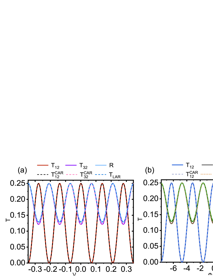
Figure 9: (color online) The transport properties of Device C. (a) The normal transmission coefficients $T_{12}$ and $T_{32}$, the CAR coefficients $T^{\mathrm{CAR}}_{12}$ and $T^{\mathrm{CAR}}_{32}$, the normal reflection coefficient $R$, and the LAR coefficient $T^{\mathrm{LAR}}$ as functions of the gate voltage $V_{g}$, with the parameters $\mu_{\mathrm{QAHI}}=0.2$, $\mu_{\mathrm{tsc}}=0.55$ and $L_{v}=40a$. (b) The analytical transmission coefficients from Eqs.(29-33) versus the dynamical phase $\phi$ with $\theta=1.07$ and an initial phase $\phi_{0}=3.26$ at the zero gate voltage.

Now let us investigate the control of Majorana fermions via Device C when the TSC is in the $\mathcal{N}=1$ phase. Considering that a Dirac electron injects from Lead-2, which is tantamount to two Majorana fermions $\gamma_{1}$ and $\gamma_{2}$. One of the two Majorana fermions, $\gamma_{2}$, passes through the right TSC, gets a dynamical phase $\phi$ in the gating QAHI region, and splits two Majorana fermions $\gamma_{L}$ and $\gamma_{3}$ with $\gamma_{L}=\gamma_{2}\sin\phi$ and $\gamma_{3}=\gamma_{2}\cos\phi$. The dynamical phase $\phi$ can control trajectories of Majorana fermion $\gamma_{2}$. Then $\gamma_{L}$ passes through the left TSC into Lead-1 and $\gamma_{3}$ counterclockwise travels along the edge of central QAHI to a contact junction. At the contact junction, the mode, $a_{d}=\frac{\sqrt{2}}{2}\gamma_{3}$, can partially exit leftward into Lead-2 or rightward into Lead-3 [see Fig.1(c)]. Recall that the other Majorana fermion $\gamma_{1}$ is reflected at the boundary of QAHI-right TSC, directly goes to the contact junction with $a_{u}=\frac{\sqrt{2}}{2}\gamma_{1}$, and splits into two branches into Lead-2 and Lead-3. Considering the current conservation, the unitary scattering matrix at the contact junction can be set as

$$\left(\begin{array}[]{cc}b_{R}\\ b_{3}\\ \end{array}\right)=\left(\begin{array}[]{cc}t&re^{-i\theta}\\ -re^{i\theta}&t\\ \end{array}\right)\left(\begin{array}[]{cc}a_{d}\\ a_{u}\\ \end{array}\right),$$ (28)

where $t$ and $r$ respectively represent the tunneling amplitude and reflection amplitude with $r^{2}+t^{2}=1$ and $\theta$ depicts an additional phase passing through the junction. To be summarized, we list all six transmission coefficients of Device C as follows:

$$\displaystyle T_{12} = T^{\mathrm{CAR}}_{12}=(1/4)\sin^{2}\phi,$$ (29)

$$\displaystyle T_{32} = [(t-r\cos\phi\sin\theta)^{2}+(r\cos\phi\cos\theta)^{2}]/4,$$ (30)

$$\displaystyle T^{\mathrm{CAR}}_{32} = [(t+r\cos\phi\sin\theta)^{2}+(r\cos\phi\cos\theta)^{2}]/4,$$ (31)

$$\displaystyle R_{2} = [(t\cos\phi+r\sin\theta)^{2}+(r\cos\theta)^{2}]/4,$$ (32)

$$\displaystyle T^{\mathrm{LAR}}_{2} = [(t\cos\phi-r\sin\theta)^{2}+(r\cos\theta)^{2}]/4.$$ (33)

In the zero tunneling limit ($t=0$ and $r=1$), the Majorana fermion $\gamma_{3}$ totally enters into Lead-3 while the mode $\gamma_{1}$ is totally reflected to Lead-2, that is, Device C is reverted into Device A. In the entire tunneling limit ($t=1$ and $r=0$), conversely, $\gamma_{3}$ goes into Lead-2 while $\gamma_{1}$ goes into Lead-3. Except for these two limiting cases, the four-side junction could mix $\gamma_{3}$ and $\gamma_{1}$, leading to that $T_{32}\not=T^{\mathrm{CAR}}_{32}$ and $R_{2}\not=T^{\mathrm{LAR}}_{2}$ as usual.

The numerical and analytical transmission and Andreev reflection coefficients of Device C with moderate coupling are plotted in Figs.9(a and b). For clear visibility, the tunneling probability $t^{2}$ and reflection strength $r^{2}$ of the contact junction are adjusted slightly away from 0.5. Apparently, the normal transmission coefficients, normal reflection coefficient, LAR and CAR coefficients, all periodically oscillate with the gate voltage $V_{g}$. The oscillation amplitudes of these coefficients are quite large as shown in Fig.9(a). It proves that the propagating route of the chiral Majorana fermion can well be regulated and controlled by the electric gate. In the analytical results in Fig.9(b), we set $\theta=1.07$ and introduce an initial phase $\phi_{0}$ without gating, that is, $\phi$ in Eqs.(29-33) is replaced by $\phi+\phi_{0}$ with $\phi_{0}=3.26$. The analytical results are in perfect agreement with the numerical ones, see Figs.9(a and b), indicating that the transport of Majorana (Dirac) fermions along the chiral edge state in TSC (QAHI) can well describe the transport process of the QAHI-TSC system.

Adopting the Landauer-Büttiker formula in Eq.(16) and the same external circuit layout in Fig.1(a) with the boundary conditions $I_{1}+I_{2}+I_{3}=0$ and $V_{1}=V_{3}$, we can achieve the linear conductance $G_{n}$ of Device C. Here the linear conductances $G_{n}$ is defined as the ratio of the current $I_{n}$ to the bias $U=V_{2}-V_{1}$ between Lead-2 and Lead-1 (Lead-3). Fig.10(a) displays the conductances $-G_{1}$, $G_{2}$ and $-G_{3}$ with the same parameter setting as Fig.9(a). Clearly, they periodically oscillate as the gate voltage $V_{g}$ varies, showing the manipulation of incoming Majorana fermions by tuning $V_{g}$. The oscillating periods of the conductances are almost identical and constant under the same $L_{v}$. From the periodic oscillation of the conductance, we can deduce the energy dispersion relation of the central QAHI marked by red squares in Fig.10(b), which is in good fit with the analytical dispersion relation.

Here we mention that conductance oscillation could be experimentally observed, which can confirm the existence of chiral Majorana edge modes and show the effective control of their propagating route. Devices B and C satisfy the aspiration of an oscillating observable. Basically, ways of observing the oscillating conductance are identical in principle, that is, to create a mixing between the incident two chiral Majorana fermions, $\gamma_{1}$ and $\gamma_{2}$. The mixing is realized by the cyclic propagating route of chiral Majorana edge modes in the central QAHI region in Device B, while in Device C, a contact junction introduces the mixing.

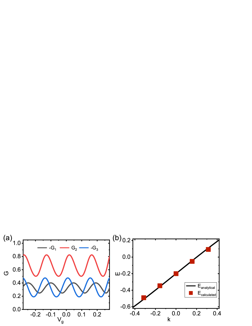
Figure 10: (color online) (a) The conductances $G_{n}$ of Device C versus the gate voltage $V_{g}$ with the same external circuit layout in the inset in Fig.1(a). The parameters are the same as Fig.9(a). (b) The energy dispersion relation of QAHI from the oscillating conductance $G_{n}$. The red squares and the black solid line are numerical and analytical results respectively.

VI the effect of potential disorder, the superconducting gap fluctuation and superconducting phase difference on the conductance oscillations

In the above, we have shown that the propagating route of chiral Majorana fermions can well be controlled by the gate voltages, which results in the oscillations of the conductance with the change of gate voltage. In the real system, impurities and disorders exist inevitably, which disrupt the transmissions of Majorana fermions and Dirac fermions. In this section, we study the effect of the potential disorder, the random spatial variation of the superconducting gap, and the non-zero superconducting phase difference between two TSCs on the oscillations of the conductance.

First, let us study the potential disorder. In order to investigate the effect of the potential disorder, we add an Anderson disorder term to the lattice Hamiltonian in Eq.(2),

$$\mathcal{H}_{\mathrm{QAHI}} = \sum_{\mathbf{i}}\left[\psi_{\mathbf{i}}^{{\dagger}}T_{0}\psi_{\mathbf{i}}+\psi_{\mathbf{i}}^{{\dagger}}w_{\mathbf{i}}\sigma_{0}\psi_{\mathbf{i}}\right.$$ (34)

$$\left.+(\psi_{\mathbf{i}}^{{\dagger}}T_{x}\psi_{\mathbf{i}+\delta\mathbf{x}}+\psi_{\mathbf{i}}^{{\dagger}}T_{y}\psi_{\mathbf{i}+\delta\mathbf{y}})+\mathrm{H.c.}\right],$$

where the new term $\psi_{\mathbf{i}}^{{\dagger}}w_{\mathbf{i}}\sigma_{0}\psi_{\mathbf{i}}$ describes the potential disorder. At each site $\mathbf{i}$, $w_{\mathbf{i}}$ is uniformly distributed in the interval [$-W_{\mathrm{sd}}$/2, $W_{\mathrm{sd}}$/2], where $W_{\mathrm{sd}}$ denotes the strength of disorder. Here we consider that the disorder exists in the whole central scattering. Take Device B for example, the disorder can exist in the left TSC, the center QAHI and the right TSC regions. For each non-zero $W_{\mathrm{sd}}$, the conductance curves are averaged over 1000 random disorder configurations. In fact, the average over the disorder configurations is equivalent to the dephasing effect.Chen et al. (2011) In Sec.IV, we have shown that the conductance of Device B oscillates with the gate voltage $V_{gu}$ in the absence of the disorder, see Fig.8(a). Now we study the effect of disorder on the conductance oscillations. Fig.11(a) shows the conductance $G$ of Device B versus the gate voltage $V_{gu}$ for the different disorder strength $W_{\mathrm{sd}}$. In the weak disorder, the oscillations of the conductance, including the oscillation amplitude and period, are almost not changed. The conductance curve of the disorder strength $W_{\mathrm{sd}}=0.1$ (the yellow dash line in Fig.11(a)) almost coincides with the curve of $W_{\mathrm{sd}}=0$ (the red solid line in Fig.11(a)). With the increase of the disorder strength $W_{\mathrm{sd}}$, the amplitude of conductance oscillations slightly reduces. But the conductance oscillations can well survive even if the disorder strength $W_{\mathrm{sd}}$ reaches $0.4$, which is close to the superconducting gap $\Delta$ and the mass gap $|m|$ of the QAHI. In fact, the conductance oscillation originates from both the chiral Dirac edge states in the QAHI region and the chiral Majorana edge modes in the TSC region, so it is very robust against the disorder. In particular, the period of the conductance oscillations is almost not affected by the disorder. For example, the oscillation period at $W_{\mathrm{sd}}=0.4$ is still equal to that at $W_{\mathrm{sd}}=0$. So even in the strong disorder, we can still obtain the dispersion relation of chiral Dirac edge states of the QAHI from the oscillation curves of the conductance versus the gate voltage.

Next, we study the effect of the superconducting gap fluctuation on the conductance oscillations. In the experiments, it is difficult to keep that the superconducting gap is perfectly uniform in real space. Usually, there are some random fluctuations. Here we consider that the superconducting gap in Eq.(3) depends on the spatial site index $\mathbf{i}$. The superconducting gap $\Delta_{\mathbf{i}}$ at the site $\mathbf{i}$ is assumed to be uniformly distributed in the interval [$\Delta-\Delta_{d}/2$, $\Delta+\Delta_{d}/2$ ], where $\Delta$ is the homogeneous superconducting gap without spatial variation and $\Delta_{d}$ denotes the strength of spatial variation. Fig.11(b) shows the conductance of Device B versus the gate voltage $V_{gu}$ for each different $\Delta_{d}$. One can clearly see that the conductance oscillation is robust against the fluctuation of the superconducting gap in real space. With the increase of the variation strength $\Delta_{d}$, the oscillation amplitude slightly decreases and the oscillation period can almost be the same as that at $\Delta_{d}=0$. When $\Delta_{d}=0.7$ (i.e. $\Delta_{\mathbf{i}}$ is uniformly distributed from $0$ to $0.7$), the conductance oscillation can still survive. If $\Delta_{d}$ increases further or the region with $\Delta_{\mathbf{i}}=0$ enlarges further, the large region in the $\mathcal{N}=1$ TSC phase is tremendously destroyed, and then the conductance oscillation disappears. These results indicate that the proposed scheme to manipulate the chiral Majorana fermions is still effective when the superconducting gap is not uniform in real space.

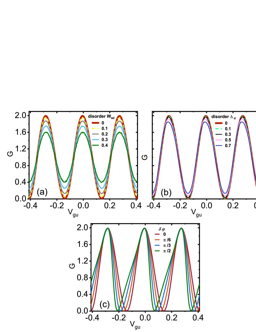
Figure 11: (a) and (b) are the linear conductance $G$ of Device B versus the upper gate voltage $V_{gu}$ for the different disorder strength $W_{\mathrm{sd}}$ and the different spatial variation of the superconducting gap $\Delta_{d}$, respectively. For each $W_{\mathrm{sd}}$ or $\Delta_{d}$, the conductance curves are averaged over 1000 random configurations. (c) is $G$ of Device B versus $V_{gu}$ for the different superconducting phase difference $\delta\varphi$. The red solid curves in (a-c) are the same as the curve in Fig.8(a). All other unmentioned parameters are the same as Fig.8(a).

In the above, we set that the superconducting phase difference $\delta\varphi$ between two TSCs is zero for a clear description. Below, let us study the effect of the non-zero $\delta\varphi$ on the conductance oscillations. When $\delta\varphi$ is non-zero, the superconducting gaps $\Delta$ in the left and right TSC regions become $\Delta e^{i\varphi_{L}}$ and $\Delta e^{i\varphi_{R}}$, and $\delta\varphi=\varphi_{L}-\varphi_{R}$. In Fig.11(c), we show the linear conductance $G$ of Device B as a function of the upper gate voltage $V_{gu}$ for each different $\delta\varphi$. Except for the superconducting phase difference $\delta\varphi$, the other parameters here are exactly the same as Fig.8(a). One can see that the oscillation of the conductance versus the gate voltage always exists regardless of the phase difference $\delta\varphi$. It clearly indicates that even in the non-zero $\delta\varphi$, our proposed scheme to control the propagating trajectories of Majorana fermions is still effective.

Finally, we discuss the parameters in real materials. In 2013, Chang et al. have successfully realized the QAHI in the Cr-$\mathrm{(Bi,Sb)_{2}Te_{3}}$ films. In this material, the Fermi velocity $\hbar v_{F}$ is about $260\ \mathrm{meV\ nm}$.Chang et al. (2013); Wang et al. (2015b) So we can determine the value of $A$, $A=\hbar v_{F}=260\ \mathrm{meV\ nm}$. Then we choose the lattice constant as $a=0.26\ \mu\mathrm{m}$. Under this condition, the dimensionless superconducting gap $\Delta=0.35$ corresponds to a real value $\Delta=0.35\ \mathrm{meV}$. It is achievable because the proximity induced superconducting gap of $\mathrm{Bi}_{2}\mathrm{Se}_{3}$ films on the $\mathrm{Nb}\mathrm{Se}_{2}$ substrate can reach $\Delta=0.5\ \mathrm{meV}$ even at 4.2K.Wang et al. (2012, 2015b) Besides, the dimensionless mass gap $m=-0.5$ corresponds to a real value $m=-0.5\mathrm{meV}$. The QAH effect in Cr-$\mathrm{(Bi,Sb)_{2}Te_{3}}$ is measured at $\mathcal{T}=30\mathrm{mK}$,Chang et al. (2013) the bulk gap of QAHI is of the order of meV, in the same magnitude as our approximation. In addition, the bulk gap of QAHI depends on the thickness of the films, so $m$ can well be tuned in experiments. Also, the size of each TSC region (100$a$, 80$a$) corresponds to (26$\mu$m, 20.8$\mu$m), which could be experimentally fabricated, compared to recent work by He et al..He et al. (2017) Besides, the size of gating QAHI region (20$a$, 20$a$) corresponds to (5.2$\mu$m, 5.2$\mu$m) and the oscillating period of conductance is about 0.2 mV of Device C and 0.4 mV of Device B, that is, the oscillation is visible when the scanning voltage is in the accuracy of $\mu$V. In the above calculation, the temperature is set to zero. In this case, the energy of the incident electron is fixed at $E=0$. At a finite temperature $\mathcal{T}$, the energy of the incident electron is distributed about in the range (-$k_{B}\mathcal{T}$, $k_{B}\mathcal{T}$). Then the oscillation amplitude reduces because of the participation of non-zero energy incident electrons, but the oscillation period can still remain the same as that at the zero temperature. At the low finite temperature (e.g. the temperature is an order of magnitude lower than the superconductor gap), the conductance oscillation can be clearly visible. So the oscillations of the conductance should be experimentally observed in the present technologies.

VII conclusion

In summary, we design three devices to manipulate chiral Majorana edge modes, within the framework of QAHI-TSC-QAHI-TSC-QAHI junction. The non-equivalent topology of the $\mathcal{N}=1$ TSC and the $\mathcal{C}=1$ QAHI separates the two Majorana modes, derived from the incoming regular electron mode. Then via the external gate voltage, a dynamical phase is induced to control trajectories of the chiral Majorana fermion in the planned Device A, leading to the oscillation of transmission coefficients. Moreover, the following Devices B and C reach an achievement of observable oscillation of the conductance, which could be detected in real experiments. The oscillating conductance is robust against the disorder and the random spatial variation of the superconducting gap due to the topological protection of chiral edge states. The stable oscillation period could also be utilized to deduce the energy dispersion relation of the chiral Dirac edge mode of the QAHI region. In addition, this periodically oscillating conductance versus the gate voltage conspicuously verify the existence of chiral Majorana edge modes, which would never appear in any classical interpretation.

References

- Alicea (2012) J. Alicea, Rep. Prog. Phys. 75, 076501 (2012).
- Beenakker (2013) C. Beenakker, Annu. Rev. Condens. Matter Phys. 4, 113 (2013).
- Elliott and Franz (2015) S. R. Elliott and M. Franz, Rev. Mod. Phys. 87, 137 (2015).
- Read and Green (2000) N. Read and D. Green, Phys. Rev. B 61, 10267 (2000).
- Kitaev (2001) A. Y. Kitaev, Phys.-Usp. 44, 131 (2001).
- Fu and Kane (2008) L. Fu and C. L. Kane, Phys. Rev. Lett. 100, 096407 (2008).
- Cook and Franz (2011) A. Cook and M. Franz, Phys. Rev. B 84, 201105(R) (2011).
- Sun et al. (2016) H.-H. Sun, K.-W. Zhang, L.-H. Hu, C. Li, G.-Y. Wang, H.-Y. Ma, Z.-A. Xu, C.-L. Gao, D.-D. Guan, Y.-Y. Li, C. Liu, D. Qian, Y. Zhou, L. Fu, S.-C. Li, F.-C. Zhang, and J.-F. Jia, Phys. Rev. Lett. 116, 257003 (2016).
- Mourik et al. (2012) V. Mourik, K. Zuo, S. M. Frolov, S. Plissard, E. P. Bakkers, and L. P. Kouwenhoven, Science 336, 1003 (2012).
- Zhang et al. (2018) H. Zhang, C.-X. Liu, S. Gazibegovic, D. Xu, J. A. Logan, G. Wang, N. van Loo, J. D. S. Bommer, M. W. A. de Moor, D. Car, R. L. M. O. H. Veld, P. J. van Veldhoven, S. Koelling, M. A. Verheijen, M. Pendharkar, D. J. Pennachio, B. Shojaei, J. S. Lee, C. J. Palmstrom, E. P. A. M. Bakkers, S. Das Sarma, and L. P. Kouwenhoven, Nature (London) 556, 74 (2018).
- Choy et al. (2011) T.-P. Choy, J. M. Edge, A. R. Akhmerov, and C. W. J. Beenakker, Phys. Rev. B 84, 195442 (2011).
- Klinovaja et al. (2013) J. Klinovaja, P. Stano, A. Yazdani, and D. Loss, Phys. Rev. Lett. 111, 186805 (2013).
- Nadj-Perge et al. (2014) S. Nadj-Perge, I. K. Drozdov, J. Li, H. Chen, S. Jeon, J. Seo, A. H. MacDonald, B. A. Bernevig, and A. Yazdani, Science 346, 602 (2014).
- Pawlak et al. (2016) R. Pawlak, M. Kisiel, J. Klinovaja, T. Meier, S. Kawai, T. Glatzel, D. Loss, and E. Meyer, Quantum Inf. 2, 16035 (2016).
- Nayak et al. (2008) C. Nayak, S. H. Simon, A. Stern, M. Freedman, and S. Das Sarma, Rev. Mod. Phys. 80, 1083 (2008).
- Alicea et al. (2011) J. Alicea, Y. Oreg, G. Refael, F. Von Oppen, and M. P. Fisher, Nat. Phys. 7, 412 (2011).
- Stanescu and Das Sarma (2018) T. D. Stanescu and S. Das Sarma, Phys. Rev. B 97, 045410 (2018).
- Chen et al. (2018a) C.-Z. Chen, Y.-M. Xie, J. Liu, P. A. Lee, and K. T. Law, Phys. Rev. B 97, 104504 (2018a).
- Fu and Kane (2009) L. Fu and C. L. Kane, Phys. Rev. Lett. 102, 216403 (2009).
- Akhmerov et al. (2009) A. R. Akhmerov, J. Nilsson, and C. W. J. Beenakker, Phys. Rev. Lett. 102, 216404 (2009).
- Law et al. (2009) K. T. Law, P. A. Lee, and T. K. Ng, Phys. Rev. Lett. 103, 237001 (2009).
- Qi et al. (2010) X.-L. Qi, T. L. Hughes, and S.-C. Zhang, Phys. Rev. B 82, 184516 (2010).
- He et al. (2017) Q. L. He, L. Pan, A. L. Stern, E. C. Burks, X. Che, G. Yin, J. Wang, B. Lian, Q. Zhou, E. S. Choi, K. Murata, X. Kou, Z. Chen, T. Nie, Q. Shao, Y. Fan, S.-C. Zhang, K. Liu, J. Xia, and K. L. Wang, Science 357, 294 (2017).
- Lian et al. (2018a) B. Lian, X.-Q. Sun, A. Vaezi, X.-L. Qi, and S.-C. Zhang, Proc. Natl. Acad. Sci. 115, 10938 (2018a).
- Zhou et al. (2019) Y.-F. Zhou, Z. Hou, and Q.-F. Sun, Phys. Rev. B 99, 195137 (2019).
- Yu et al. (2010) R. Yu, W. Zhang, H.-J. Zhang, S.-C. Zhang, X. Dai, and Z. Fang, Science 329, 61 (2010).
- Chang et al. (2013) C.-Z. Chang, J. Zhang, X. Feng, J. Shen, Z. Zhang, M. Guo, K. Li, Y. Ou, P. Wei, L.-L. Wang, Z.-Q. Ji, Y. Feng, S. Ji, X. Chen, J. Jia, X. Dai, Z. Fang, S.-C. Zhang, K. He, Y. Wang, L. Lu, X.-C. Ma, and Q.-K. Xue, Science 340, 167 (2013).
- Kou et al. (2014) X. Kou, S.-T. Guo, Y. Fan, L. Pan, M. Lang, Y. Jiang, Q. Shao, T. Nie, K. Murata, J. Tang, Y. Wang, L. He, T.-K. Lee, W.-L. Lee, and K. L. Wang, Phys. Rev. Lett. 113, 137201 (2014).
- Chang et al. (2015) C.-Z. Chang, W. Zhao, D. Y. Kim, H. Zhang, B. A. Assaf, D. Heiman, S.-C. Zhang, C. Liu, M. H. Chan, and J. S. Moodera, Nat. Mater. 14, 473 (2015).
- Sun and Jia (2017) H.-H. Sun and J.-F. Jia, Sci. China: Phys., Mech. Astron. 60, 057401 (2017).
- Chung et al. (2011) S. B. Chung, X.-L. Qi, J. Maciejko, and S.-C. Zhang, Phys. Rev. B 83, 100512(R) (2011).
- Ji and Wen (2018) W. Ji and X.-G. Wen, Phys. Rev. Lett. 120, 107002 (2018).
- Huang et al. (2018) Y. Huang, F. Setiawan, and J. D. Sau, Phys. Rev. B 97, 100501(R) (2018).
- Lian et al. (2018b) B. Lian, J. Wang, X.-Q. Sun, A. Vaezi, and S.-C. Zhang, Phys. Rev. B 97, 125408 (2018b).
- Andreev (1966) A. F. Andreev, Zh. ksp. Teor. Fiz. 49, 655 (1965) [Sov. Phys. JETP 22, 455 (1966)].
- Tanaka et al. (2009) Y. Tanaka, T. Yokoyama, and N. Nagaosa, Phys. Rev. Lett. 103, 107002 (2009).
- Hou et al. (2016) Z. Hou, Y. Xing, A.-M. Guo, and Q.-F. Sun, Phys. Rev. B 94, 064516 (2016).
- Deutscher and Feinberg (2000) G. Deutscher and D. Feinberg, Appl. Phys. Lett. 76, 487 (2000).
- Wang et al. (2015a) J. Wang, L. Hao, and K. S. Chan, Phys. Rev. B 91, 085415 (2015a).
- Zhou et al. (2018a) Y.-F. Zhou, Z. Hou, P. Lv, X. Xie, and Q.-F. Sun, Sci. China: Phys., Mech. Astron. 61, 127811 (2018a).
- Zhang et al. (2017) Y.-T. Zhang, Z. Hou, X. C. Xie, and Q.-F. Sun, Phys. Rev. B 95, 245433 (2017).
- Zhou et al. (2018b) Y.-F. Zhou, Z. Hou, Y.-T. Zhang, and Q.-F. Sun, Phys. Rev. B 97, 115452 (2018b).
- Chen et al. (2018b) C.-Z. Chen, J. J. He, D.-H. Xu, and K. T. Law, Phys. Rev. B 98, 165439 (2018b).
- Li et al. (2019) C.-A. Li, J. Li, and S.-Q. Shen, Phys. Rev. B 99, 100504(R) (2019).
- Wang and Lian (2018) J. Wang and B. Lian, Phys. Rev. Lett. 121, 256801 (2018).
- Zeng et al. (2018) Y. Zeng, C. Lei, G. Chaudhary, and A. H. MacDonald, Phys. Rev. B 97, 081102(R) (2018).
- Datta (1995) S. Datta, Electronic Transport in Mesoscopic Systems (Cambridge University Press, 1995).
- Bernevig and Hughes (2013) B. A. Bernevig and T. L. Hughes, Topological insulators and topological superconductors (Princeton university press, 2013).
- Schnyder et al. (2008) A. P. Schnyder, S. Ryu, A. Furusaki, and A. W. W. Ludwig, Phys. Rev. B 78, 195125 (2008).
- Cheng et al. (2009) S.-G. Cheng, Y. Xing, J. Wang, and Q.-F. Sun, Phys. Rev. Lett. 103, 167003 (2009).
- Sun et al. (1999) Q.-F. Sun, J. Wang, and T.-H. Lin, Phys. Rev. B 59, 3831 (1999).
- Sun and Xie (2009) Q.-F. Sun and X. C. Xie, J. Phys.-Condes. Matter 21, 344204 (2009).
- Qi et al. (2019) J. Qi, H. Liu, C.-Z. Chen, H. Jiang, and X. C. Xie, Sci. China: Phys., Mech. Astron. 63, 227811 (2019).
- Chen et al. (2011) J.-C. Chen, H. Zhang, S.-Q. Shen, and Q.-F. Sun, J. Phys.-Condes. Matter 23, 495301 (2011).
- Wang et al. (2015b) J. Wang, Q. Zhou, B. Lian, and S.-C. Zhang, Phys. Rev. B 92, 064520 (2015b).
- Wang et al. (2012) M.-X. Wang, C. Liu, J.-P. Xu, F. Yang, L. Miao, M.-Y. Yao, C. L. Gao, C. Shen, X. Ma, X. Chen, Z.-A. Xu, Y. Liu, S.-C. Zhang, D. Qian, J.-F. Jia, and Q.-K. Xue, Science 336, 52 (2012).