∎
11institutetext: ∗ Corresponding author: D Akdemir 22institutetext: University College Dublin, Ireland
22email: deniz.akdemir.work@gmail.com
Adventures in Multi-Omics I:
Combining heterogeneous data sets via relationships matrices††thanks: This research was supported by WheatSustain.
Abstract
In this article, we propose a covariance based method for combining partial data sets in the genotype to phenotype spectrum. In particular, an expectation-maximization algorithm that can be used to combine partially overlapping relationship/covariance matrices is introduced. Combining data this way, based on relationship matrices, can be contrasted with a feature imputation based approach. We used several public genomic data sets to explore the accuracy of combining genomic relationship matrices. We have also used the heterogeneous genotype/phenotype data sets in the https://triticeaetoolbox.org/ to illustrate how this new method can be used in genomic prediction, phenomics, and graphical modeling.
Keywords:
Multi-Omics Phenomics Breeding Complex traits Genomic selection Genome-wide markers Kernel-regression Multiple kernel learning Mixed models Imputation Covariance Estimation Expectation-MaximizationKey message: Several covariance matrices obtained from independent experiments can be combined as long as these matrices are partially overlapping. We demonstrate the usefulness of this methodology with examples in combining data from several partially linked genotypic and phenotypic experiments.
Conflict of interest: The authors declare that there is no conflict of interest.
Author contribution statement:
-
•
DA: Conception or design of the work, statistics, programs, and simulations, drafting the article, critical revision of the article.
-
•
JIS: Drafting the article, critical revision of the article.
1 Introduction
The area of genomic prediction, i.e. predicting an organism´s phenotype using genetic information (Meuwissen et al., 2001), is a cutting edge tool. It is used by many breeding companies, because it improves three out of the four factors affecting the breeder's equation (Hill and Mackay, 2004). It reduces generation interval, improves accuracy of selection and increase selection intensity for a fixed budget when comparing with marker-assisted selection or phenotypic selection (Desta and Ortiz, 2014; Heffner et al., 2011, 2010; Juliana et al., 2018; de los Campos et al., 2013). Genomic selection (GS) and prediction are in a continuous progressing tool that promises to help to meet the human food challenges in the next decades (Crossa et al., 2017). Genome-wide associating mapping studies, which originated in human genetics (Bodmer, 1986; Risch and Merikangas, 1996; Visscher et al., 2017), has also become a routine in plant breeding (Gondro et al., 2013).
The rapid scientific progress in these genomics studies was due to the decrease in genotyping costs by the development of next generating sequencing platforms after 2007 (Mardis, 2008a, b). High-throughput instruments are routinely used in laboratories in basic science applications, which led to the democratization of genome-scale technologies. The biological data generated in the last few years have growth exponentially which led to a high dimensional and unbalanced nature of the ’omics’ data, in the forms of marker and sequence information; expression, metabolomics, microbiome data, classical phenotype data, image-based phenotype data (Bersanelli et al., 2016). Private and public breeding programs, as well as companies and universities, have developed different genomics technology which has resulted in the generation of unprecedented levels of sequence data, which bring new challenges in terms of data management, query, and analysis.
It is clear that detailed phenotype data, combined with increasing amounts of genomic data, have an enormous potential to accelerate the identification of key traits to improve our understanding of quantitative genetics (Crossa et al., 2017). Nevertheless, one of the challenges that still need to be addressed is the incompleteness inherent in these data, i.e., several types of genomic/phenotypic information which might each covering only a few of the genotypes under study (Berger et al., 2013). Data harmonization enables cross-national and international comparative research, as well as allows the investigation of whether or not data sets have similarities. In this paper, we address the complex issue of the high degree of dimensional and unbalanced nature of the omics data by studying how we can combine data generated from different sources and facilitating data integration and interdisciplinary research. The increase of sample size and the improvement of generalizability and validity of research results constitute the most significant benefits of the harmonization process. The ability to effectively harmonize data from different studies and experiments facilitates the rapid extraction of new scientific knowledge.
One way to approach the incompleteness and the disconnection among datasets is to combine the relationship information learned from these dataset. The statistical problem addressed in this paper is the calculation of a combined covariance matrix from incomplete and partially-overlapping pieces of covariance matrices that were obtained from independent experiments. We assume that the data is a random sample of partial covariance matrices from a Wishart distribution, then we derive the expectation-maximization algorithm for estimating the parameters of this distribution. According to our best knowledge no such statistical methodology exists, although the proposed method has been inspired by similar methods such as (conditional) iterative proportional fitting for the Gaussian distribution (Cramer, 1998, 2000) and a method for combining a pedigree relationship matrix and a genotypic matrix relationship matrix which includes a subset of genotypes from the pedigree-based matrix (Legarra et al., 2009) (namely, the H-matrix). The applications in this paper are chosen in the area of plant breeding and genetics. However, the statistical method is applicable much beyond the described examples in this article.
2 Methods and Materials
2.1 Statistical methods for combining incomplete data
2.1.1 Imputation
The standard method of dealing with heterogeneous data involves the imputation of features (Shrive et al., 2006). If the data sets to be combined overlap over a substantial number of features then the unobserved features in these data sets can be accurately imputed based on some imputation method (Rutkoski et al., 2013).
Imputation step can be done using many different methods: Several popular approaches include random forest (Breiman, 2001) imputation, expectation maximization based imputation (Endelman, 2011), low-rank matrix factorization methods that are implemented in the R package (Hastie and Mazumder, 2015). In addition, parental information can be used to improve imputation accuracies (Nicolazzi et al., 2013; Gonen et al., 2018; VanRaden et al., 2015; Browning and Browning, 2009). In this study, we used the low-rank matrix factorization method in all of the examples which included an imputation step. The selection of this method was due to computational burden of the other alternatives.
2.1.2 Combining genomic relationship matrices
In this section, we describe the Wishart EM-Algorithm for combining partial genetic relationship matrices111In what follows, we will refer to genetic relationship matrices that measure how genotypes are related (See Supplementary Section 5.3 for a description of how to calculate a genetic relationship matrix from genome-wide markers (genomic relationship matrix)). However, a theme in this article is that a genetic relationship matrix is a special kind of covariance matrix. Therefore, the same arguments below apply to covariance matrices that measure the relationship between traits or features..
Wishart EM-Algorithm for Estimation of a Combined Relationship Matrix from Partial Samples
Let be the set of not necessarily disjoint subsets of genotypes covering a set of (i.e., ) with total genotypes. Let be the corresponding sample of genetic relationship matrices.
Starting from an initial estimate the Wishart EM-Algorithm repeats updating the estimate of the genetic relationship matrix until convergence:
| (1) |
where is the set of genotypes in the given partial genomic relationship matrix and is the set difference of and The matrices are permutation matrices that put each matrix in the sum in the same order. The initial value, is usually assumed to be an identity matrix of dimesion The estimate at the last iteration converts to the estimated genomic relationship with
A weighted version of this algorithm can be obtained replacing in Equation 1 with for a vector of weights
Derivation of the Wishart-EM algorithm and and its asymptotic errors are given in Supplementary.
2.2 Materials: Data sets and Experiments.
In this section, we describe the data sets and the experiments we have designed to explore and exploit the Wishart EM-Algorithm.
Note that the examples in the main text involve real data sets and validation with such data can only be as good as the ground truth known about the underlying system. We also included several simulation studies in the supplementary (Supplementary Example 1 and 2) using simulated data to show that the algorithm performs as expected (maximizes the likelihood and provides a ’good’ estimate of the parameter values) when the ground truth is known.
Example 1- Potato Data set; when imputation is not an option. Anchoring independent pedigree-based relationship matrices using a genotypic relation matrix
The Wishart EM-Algorithm can be used when the imputation of the original genomic features is not feasible. For instance, it can be used to combine partial pedigree-based relationship matrices with marker-based genomic relationship matrices. In this example, we demonstrate that genomic relationship matrices can be used to connect several pedigree-based relationship matrices.
The data set is cited in (Endelman et al., 2018) and is available in the R Package AGHmatrix (Rampazo Amadeu et al., 2016). It consists of the pedigree of 1138 potato genotypes, 571 of these genotypes also have data for 3895 tetraploid markers. The pedigree-based relationship matrix A was calculated with R package AGHmatrix (Rampazo Amadeu et al., 2016) using pedigree records, there were 185 founders (clones with no parent).
At each replication of the experiment, two non-overlapping pedigree-based relationship matrices each with the sample size genotypes selected at random from the were 571 genotypes were generated. In addition, a genotypic relationship matrix was obtained for a random sample of genotypes selected at random half from the genotypes in the first pedigree and a half from the genotypes from the second pedigree. These genetic relationship matrices were combined to get a combined genetic relationship matrix (See Figure 1). This combined relationship matrix was compared to the pedigree-based relationship matrix of the corresponding genotypes using mean squared errors and Pearson’s correlations. This experiment was repeated 30 times for each pair.
Example 2 - Rice data set. Combining independent low density marker data sets
Rice data set was downloaded from www.ricediversity.org. After curation, the marker data set consisted of 1127 genotypes observed for 387161 markers.
In each instance of the experiment, the number of kernel marker data sets with 200 genotypes and 2000 markers were created by randomly sampling the genotypes and markers in each genotype file. These data sets were combined using the Wishart EM-Algorithm and also by imputation to give two genomic relationship matrices. For the totality of genotypes in these combined data sets, we also randomly sampled 2000, 5000 or 10000 markers and calculated the genomic relationships based on these marker subsets. All of these genomic relationship matrices were compared with the corresponding elements of the relationship matrix based on the entire genomic data by calculating the mean squared error between the upper diagonal elements including the diagonals. This experiment was repeated 20 times.
Example 3 - Wheat Data at Triticale Toolbox. Combining genomic data sets to use in genomic prediction.
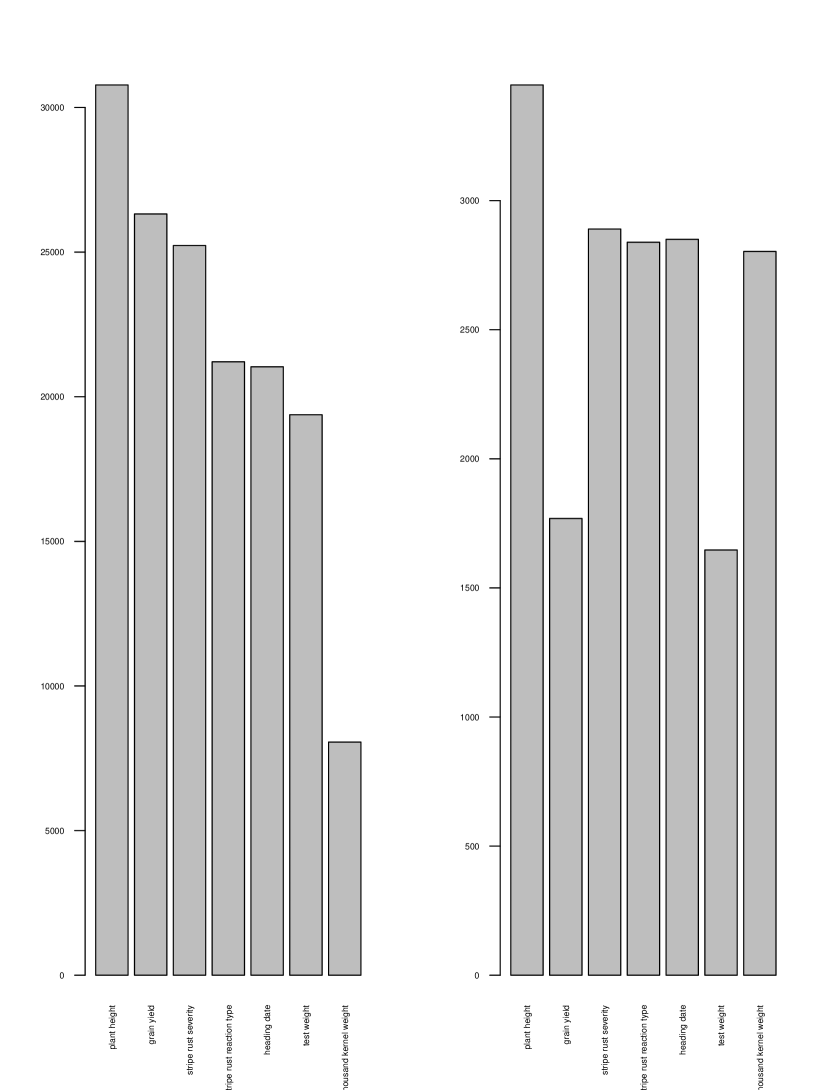
This example involves estimating breeding values for seven economically important traits for 9102 wheat lines obtained by combining publicly available genotypic data sets. The genotypic and phenotypic data were downloaded from the triticale toolbox database. Each of the marker data sets was pre-processed to produce the corresponding genomic relationship matrices. Table 1 and Supplementary Figure S6 describes the phenotypic records and number of distinct genotypes for each trait.
| Label | Data | # Genotypes | # Markers |
| d1 | 2012_SRWW_ElitePanel | 276 | 90782 |
| d2 | 2014_HAPMAP | 53 | 180198 |
| d3 | 2014_SRWW_YNVP | 307 | 109073 |
| d4 | 2014_TCAPABBSRWMID | 365 | 100340 |
| d5 | CornellMaster_2013 | 1128 | 18846 |
| d6 | Dart_NebDuplicates_2010 | 278 | 1970 |
| d7 | HWWAMP_2013 | 288 | 32288 |
| d8 | HWWAMP_2014 | 311 | 265551 |
| d9 | NSGC9k_spring | 2196 | 5303 |
| d10 | NSGC9k_winter | 1674 | 5010 |
| d11 | TCAP90k_HWWAMP_SPRN | 20 | 16842 |
| d12 | TCAP90k_LeafRust | 339 | 24610 |
| d13 | TCAP90k_NAMparents | 60 | 25851 |
| d14 | TCAP90k_SpringAm | 248 | 24343 |
| d15 | TCAP90k_SWW | 317 | 24978 |
| d16 | WWDP9k | 2258 | 6232 |
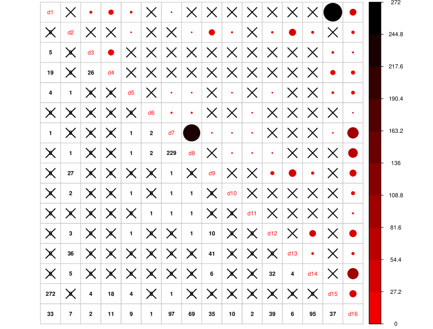
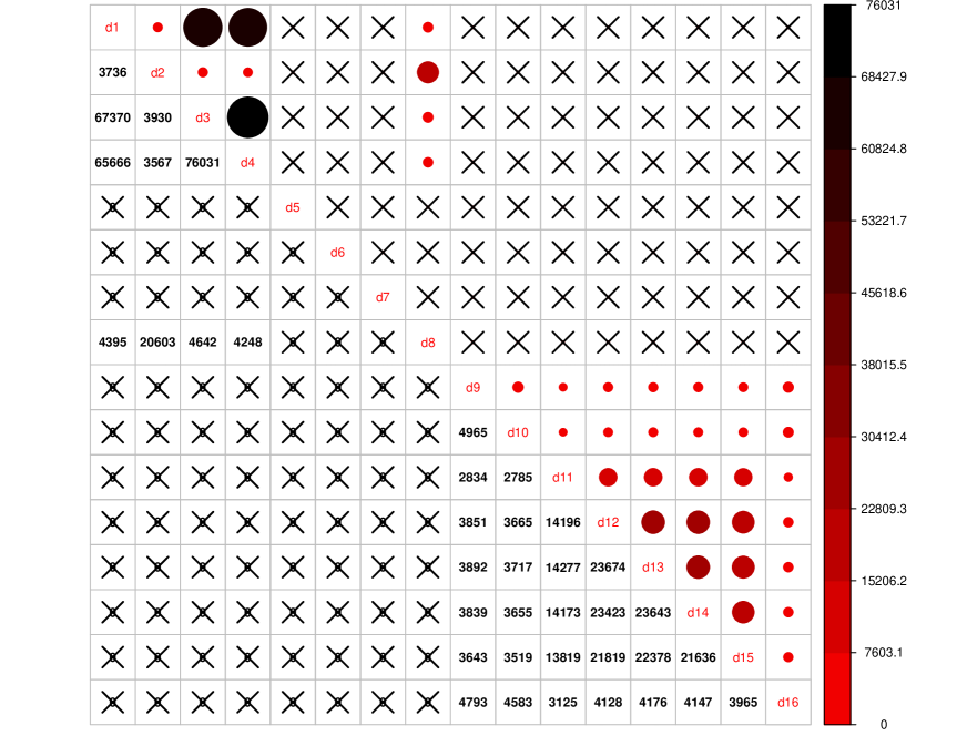
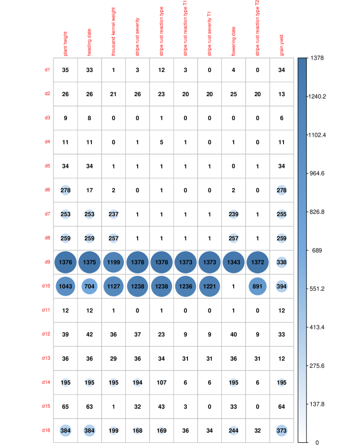
Using the combined relationship matrix we can build genomic prediction models. To test the performance of predictions based on the combined relationship matrix, we have formulated two scenarios. The intersection of genotypes among the 16 genotypic experiments is showed in Figure 2 and the intersection of common markers among genotypic experiments in Figure 3.
-
•
Cross-validation scenario 1
The first scenario involved a 10 fold cross-validation based on a random split of the data. For each trait, the available genotypes were split into 10 random folds. The GEBVs for each fold were estimated from a mixed model (see Supplementary Section 5.4 for a description of this model) that was trained on the phenotypes available for the remaining genotypes. The accuracy of the predictions was evaluated by calculating the correlations between the GEBVs and the observed trait values.
-
•
Cross-validation scenario 2 The second Cross-validation scenario involved leaving out the phenotypic records corresponding genotypes in one of the genomic data sets followed by estimation of the trait values for these genotypes based on a mixed model trained on the remaining genotypes and phenotypic records. This scenario was used for each trait, and the accuracies were evaluated by calculating the correlations between the estimated and the observed trait values within each group.
Example 4 - Wheat Data at Triticale Toolbox. Combining Phenotypic Experiments
The Wishart EM-Algorithm can also be used to combine correlation matrices222We used correlations instead of covariances because the phenotypic experiments were very heterogeneous in terms of the variances of the different traits. obtained from independent phenotypic experiments. One-hundred forty four phenotypic experiments involving 95 traits in total were selected from 2084 trials and 216 traits available at the Triticale Toolbox. In this filtered set of trials, each trial and trait combination had at least 100 observations and two traits. Furthermore, the percentage of missingness in these data sets was at most The mean and the median of the number of traits in these trials were and correspondingly (See Figure 5 and Supplementary Figure S5).
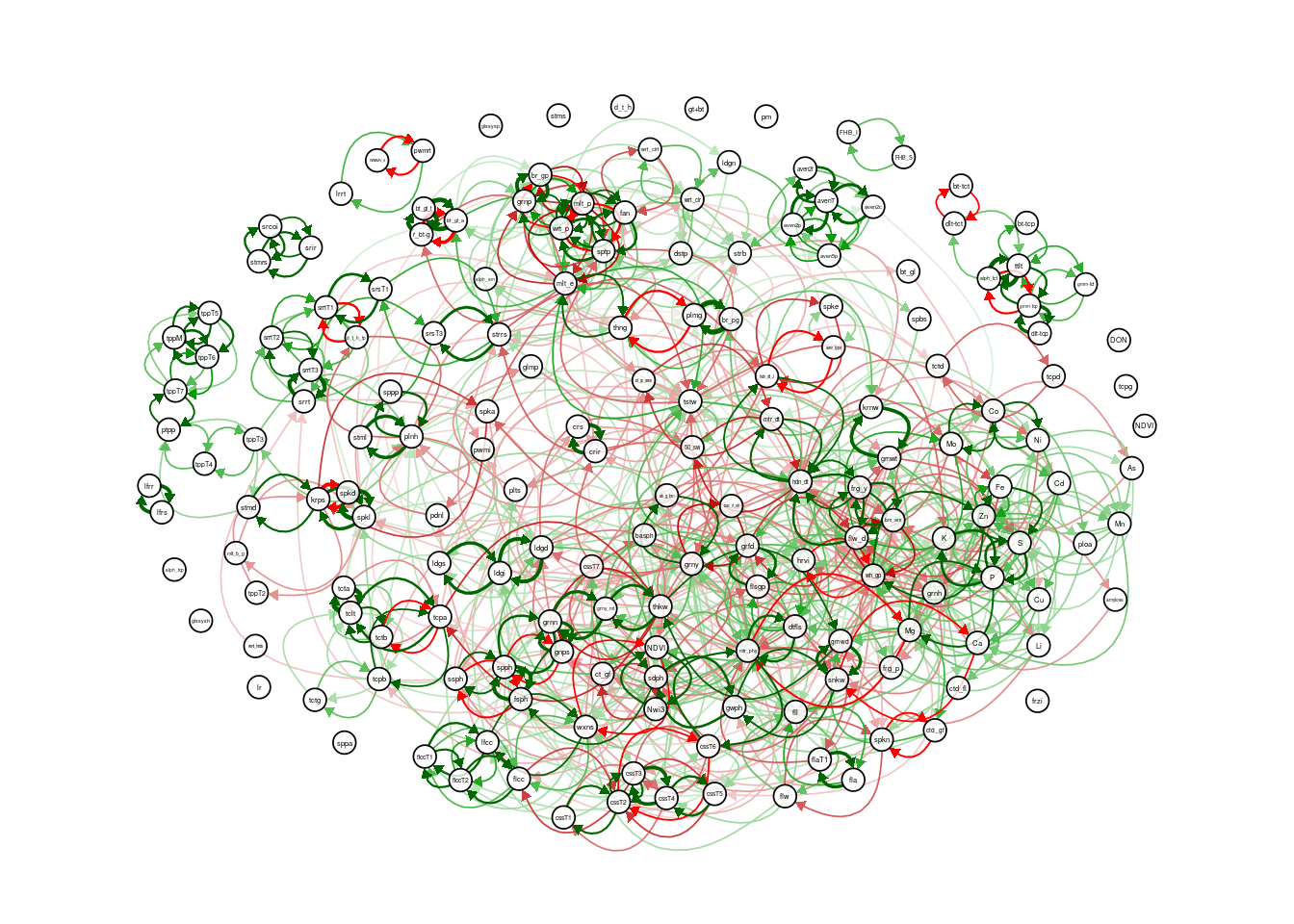
The correlation matrix for the traits in each trial was calculated and then combined using the Wishart EM-Algorithm. The resulting covariance matrix was used in learning a directed acyclic graph (DAG) using the qgraph R Package (Epskamp et al., 2012).
A more advanced example that involved combining the phenotypic correlation matrices from oat (78 correlation matrices), barley (143 correlation matrices) and wheat (144 correlation matrices) data sets downloaded and selected in a similar way as above were combined to obtain the DAG involving 196 traits in the Supplementary (Supplementary Example 6.1).
3 Results
Example 1- When imputation is not an option: Anchoring independent pedigree-based relationship matrices using a genotypic relation matrix - Potato Data
Figure 6 shows the correlation correlation and MSE results as either of the sizes of the pedigree matrices and the number of genotypes in the genomic relationship matrices increases. The MSE results for these experiments ranged from to with a mean of and the correlation values ranged from to with a mean of
Example 2 - Rice data set. Combining independent low density marker data sets
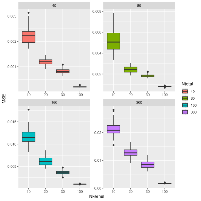
The MSE and correlation results for this experiment are given in Figure 7. In general, as the number of independent data sets increases the accuracy of the all of the methods/scenarios increases (decreasing MSEs and increasing correlations). In general, the accuracy of the Wishart EM-algorithm in terms of MSEs ranged from to with a mean value of The accuracies measured in correlation ranged from to with a mean value of For the imputation based method MSEs ranged from to (mean ) and the correlations ranged from to (mean ).

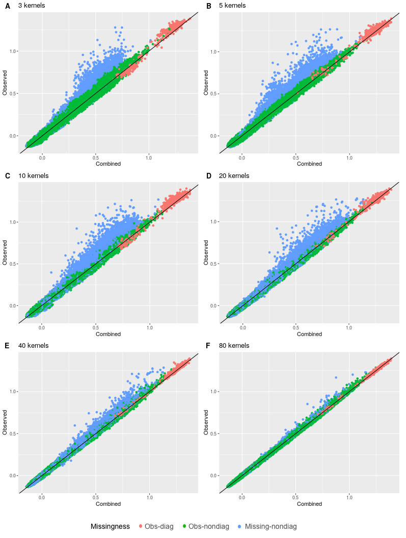
Figure 8 displays the scatter plot of full genomic relationship matrix (obtained using all 387161 markers) against the one obtained by combining a sample of partial relationship matrices (200 randomly selected genotypes and 2000 randomly selected markers each) over varying numbers of samples (3, 5, 10, 20, 40, and 80 partial relationship matrices). Observed parts (observed-diaginal and observed non-diagonal) of the genomic relationship matrix can be predicted with high accuracy and no bias. As the sample size increse, the estimates get closer to the one obtained using all of the data. We observe that the estimates of the unobserved parts of the relationship are biased towards zero but his bias quickly decreases as the sample size increases.
Example 3 - Wheat Data at Triticale Toolbox. Combining genomic data sets to use in genomic prediction
The results summarized by Figure 9 indicate that when a random sample of genotypes are selected for the test population the accuracy of the genomic predictions using the combined genomic relationship matrix can be high (Cross-validation scenario 1). Average accuracy for estimating plant height was about and for yield Lowest accuracy values were for test weight with a mean value of
The performance decreases significantly if we use between population predictions (Cross-validation scenario 2). Certain populations were harder to predict, for example, d5, d6, d9. On the other hand, some populations were easier to predict, for example, d12-d16. Average accuracy for estimating plant height was about for yield
Example 4 - Wheat Data at Triticale Toolbox- Combining Phenotypic Experiments In this example, we combined correlation matrices obtained from independent phenotypic experiments. Figures 10 and S3 displayed the correlation matrix for the traits in a directed acyclic graph (DAG) and in a heatmap, respectively. In Figure 10 each node represents a trait and each edge represents a correlation between two traits. One of the strength on this representation, is that you can elucidate the correlation between traits that you did not measured in your experiment. For example, from all the traits, grain width (grnwd) and above ground biomass (ab_g_bm) are positive correlated (blue arrows) with grain yield. In turn, grwd is highly positive correlated with biomass at maturity (bm.am) but negative correlated with harvest index (hrvi). Negative correlations (red) can also be observed among traits. Traditional inverse correlations such as protein (wh_gp) and grwd can be also observed.
Combining datasets by correlation matrices also help to group traits. Figure S3 shows two groups of positively traits. The traits in these two groups are positively correlated within the group but negatively correlated with traits in the other group. For example, we see that yield related traits such as traits grain yield, grain weight, harvest index, etc,… are positively correlated. On the other hand these traits are negatively correlated with disease related traits such as bacterial leaf streak, stripe rust traits and also with quality traits such as protein and nutrient content.
| name | label | name | label | name | label | name | label |
| aboveground biomass | ab_g_bm | fertile spikelets per head | fsph | harvest index | hrvi | seeds per head | sdph |
| As | As | flag leaf angle | fla | heading date | hdn_dt | single kernel weight | snkw |
| bacterial leaf streak | bac_lf_str | flag leaf angle T1 | flaT1 | K | K | spike length | spkl |
| basal aborted spikelets per head | basph | flag leaf chlorophyll content | flcc | leaf chlorophyll content | lfcc | spike number | spkn |
| biomass at maturity | bm_am | flag leaf chlorophyll content T1 | flccT1 | leaf rust reaction type | lrrt | spikelets per head | spph |
| Ca | Ca | flag leaf chlorophyll content T2 | flccT2 | leaf rust response | lfrr | stem rust coefficient of infection | srcoi |
| canopy senescence score T1 | cssT1 | flag leaf length | fll | leaf rust severity | lfrs | stem rust infection response | srir |
| canopy senescence score T2 | cssT2 | flag leaf stay-green period | flsgp | Li | Li | stem rust severity | stmrs |
| canopy senescence score T3 | cssT3 | flag leaf width | flw | lodging degree | ldgd | stem solidness | stms |
| canopy senescence score T4 | cssT4 | flowering date | flw_d | lodging incidence | ldgi | sterile spikelets per head | ssph |
| canopy senescence score T5 | cssT5 | forage protein | frg_p | maturity date (physiological) | mtr_phy | stripe rust reaction type | srrt |
| canopy senescence score T6 | cssT6 | forage yield | frg_y | Mg | Mg | stripe rust reaction type T1 | srrtT1 |
| canopy senescence score T7 | cssT7 | freeze injury | frzi | Mn | Mn | stripe rust reaction type T2 | srrtT2 |
| canopy temperature (grain fill) | ct_gf | glume pubescence | glmp | Mo | Mo | stripe rust reaction type T3 | srrtT3 |
| canopy temperature depression (flowering) | ctd_fl | grain fill duration | grfd | Ni | Ni | stripe rust severity | strrs |
| canopy temperature depression (grain fill) | ctd_gf | grain hardness | grnh | Normalized Difference Vegetation Index | NDVI | stripe rust severity T1 | srsT1 |
| Cd | Cd | grain number | grnn | Normalized water index 3 | Nwi3 | stripe rust severity T3 | srsT3 |
| Co | Co | grain number per spikelet | gnps | P | P | test weight | tstw |
| Cu | Cu | grain weight | grnwt | peduncle length | pdnl | thousand kernel weight | thkw |
| days to flag leaf senescence | dtfls | grain weight per head | gwph | plant height | plnh | waxiness | wxns |
| days to heading | d_t_h | grain width | grnwd | plot shattering | plts | whole grain protein | wh_gp |
| days to heading (fall planting) | d_t_h_fp | grain yield | grny | powdery mildew reaction type | pwmrt | WSBMV reaction type | WSBMV_rt |
| Fe | Fe | grain yield (main tillers) | grny_mt | S | S | Zn | Zn |
4 Discussion and conclusions
Genomic data are now relatively inexpensive to collect and phenotypes remain to be the primary way to define organisms.Many genotyping technologies exist and these technologies evolve which leads to heterogeneity of genomic data across independent experiments. Similarly, phenotypic experiments, due to the high relative cost of phenotyping, usually can focus only on a set of key traits of interest. Therefore, when looking over several phenotypic data sets, the usual case is that these data sets are extremely heterogeneous and incomplete, and the data from these experiments accumulate in databases.
This presents a challenge but also an opportunity to make the most of genomic/phenotypic data in the future. In the long term, such databases of genotypic and phenotypic information will be invaluable to scientists as they seek to understand complex biological organisms. Issues and opportunities are beginning to emerge, like the promise of gathering phenotypical knowledge from totally independent datasets for meta-analyses.
To address the challenges of genomic and phenotypic data integration, we developed a simple and efficient approach for integrating data from multiple sources. This method can be used to combine information from multiple experiments across all levels of the biological hierarchy such as microarray, gene expression, microfluidics, and proteomics will help scientists to discover new information and to develop new approaches.
For example, Figure 7 shows that we can estimate the full genomic relationship matrix more precisely from independent partially overlapping data sets of genotypes and markers each than estimating from a data set (for the combined set of genotypes) that has fixed markers. Twenty independent genomic data sets of genotypes and markers is as good as one genomic dataset with markers. When we compare it to the rest of the entries imputation is the least effective for estimating the unobserved parts of the genomic relationship matrix. This suggests that accounting for incomplete genetic relationships would be a more promising approach than estimating the genomic features by imputation and then calculating the genomic relationship matrix.
Figure 6 shows we can accurately estimate the unobserved relationships among the genotypes in two independent pedigree based relationship matrices by genotyping a small proportion of the genotypes in these data sets. For example, the mean correlation for the worst case setting ( genotypes in each pedigree and 10 from each of the pedigree genotyped) was This value increased all the way up to for the best case ( genotypes in each pedigree and from each of the pedigree genotyped).
The selection in genomic selection is based on the genomically estimated breeding values (GEBVs). A common approach to obtaining GEBVs involves the use of a linear mixed model with a marker-based additive relationship matrix. If the phenotypic information corresponding to the genotypes in one or more of the component matrices are missing then the genotypic value estimates can be obtained using the available phenotypic information and the combined genomic information that links all the genotypes and the experiments.
Imputation has been the preferred method when dealing with incomplete and data sets (Browning, 2008; Browning and Browning, 2009; Howie et al., 2011; Druet et al., 2014; Erbe et al., 2016). However, imputation can be inaccurate if the data is very heterogeneous (Van Buuren et al., 2011). In these cases, as seen in examples above, the proposed approach which uses the relationships instead of the actual features seems to outperform imputation for inferring genomic relationships. Besides, the methods introduced in this article are useful even when imputation is not feasible. For example, two partially overlapping relationship matrices, one pedigree-based and the other can be combined to make inferences about the genetic similarities of genotypes in both of these data sets.
There are also limitations to our approach. In particular, when we combine data using relationship matrices original features are not imputed. Our method may not be the best option when inferences about genomic features are needed, such as in GWAS. We can address this issue by imputing the missing features using the combined relationship matrix for example using a k-nearest neighbor imputation (Hastie et al., 2001) or by kernel smoothing. Moreover, if the marker data in the independent genomic studies can be mapped to local genomic regions, then the combined relationship matrices can be obtained for these genomic regions separately and a kernel based model such as the ones in Yang et al. (2008); Akdemir and Jannink (2015) can be used for association testing. The nature of missingness in data will affect our algorithms performance. Inference based on approaches that ignore the missing data mechanisms are valid for missing completely at random (MCAR), missing at random (MAR) but probably not for not missing at random (NMAR) (Little and Rubin, 2002; Rubin, 1976).
4.1 Software and data availability
The software was written using C++ and R. The code for replicating some of the analysis can be requested from the corresponding author.
Acknowledgements.
References
- Akdemir and Jannink (2015) Deniz Akdemir and Jean-Luc Jannink. Locally epistatic genomic relationship matrices for genomic association and prediction. Genetics, 199(3):857–871, 2015.
- Anderson (1984a) Theodore W. Anderson. An Introduction to Multivariate Statistical Analysis, 2nd Edition. Wiley, sep 1984a. ISBN 0471889873. URL https://www.xarg.org/ref/a/0471889873/.
- Anderson (1984b) TW Anderson. An Introduction to Multivariate. Wiley & Sons, 1984b.
- Berger et al. (2013) Bonnie Berger, Jian Peng, and Mona Singh. Computational solutions for omics data. Nature reviews genetics, 14(5):333–346, 2013.
- Bersanelli et al. (2016) Matteo Bersanelli, Ettore Mosca, Daniel Remondini, Enrico Giampieri, Claudia Sala, Gastone Castellani, and Luciano Milanesi. Methods for the integration of multi-omics data: mathematical aspects. BMC bioinformatics, 17(2):S15, 2016.
- Bodmer (1986) Walter F Bodmer. Human genetics: the molecular challenge. In Cold Spring Harbor symposia on quantitative biology, volume 51, pages 1–13. Cold Spring Harbor Laboratory Press, 1986.
- Breiman (2001) Leo Breiman. Random forests. Machine learning, 45(1):5–32, 2001.
- Browning and Browning (2009) Brian L Browning and Sharon R Browning. A unified approach to genotype imputation and haplotype-phase inference for large data sets of trios and unrelated individuals. The American Journal of Human Genetics, 84(2):210–223, 2009.
- Browning (2008) Sharon R Browning. Missing data imputation and haplotype phase inference for genome-wide association studies. Human genetics, 124(5):439–450, 2008.
- Cramer (1998) Erhard Cramer. Conditional iterative proportional fitting for gaussian distributions. Journal of multivariate analysis, 65(2):261–276, 1998.
- Cramer (2000) Erhard Cramer. Probability measure with given marginals and conditionals: I-projections and conditional iterative proportional fitting. Statistics & Risk Modeling, 18(3):311–330, 2000.
- Crossa et al. (2017) José Crossa, Paulino Pérez-Rodríguez, Jaime Cuevas, Osval Montesinos-López, Diego Jarquín, Gustavo de los Campos, Juan Burgueño, Juan M González-Camacho, Sergio Pérez-Elizalde, Yoseph Beyene, et al. Genomic selection in plant breeding: methods, models, and perspectives. Trends in plant science, 22(11):961–975, 2017.
- de los Campos et al. (2013) Gustavo de los Campos, John M Hickey, Ricardo Pong-Wong, Hans D Daetwyler, and Mario PL Calus. Whole-genome regression and prediction methods applied to plant and animal breeding. Genetics, 193(2):327–345, 2013.
- Dempster et al. (1977) A.P. Dempster, N.M. Laird, and D.B. Rubin. Maximum likelihood from incomplete data via the em algorithm. Journal of the Royal Statistical Society. Series B (Methodological), pages 1–38, 1977.
- Dempster et al. (1981) Arthur P Dempster, Donald B Rubin, and Robert K Tsutakawa. Estimation in covariance components models. Journal of the American Statistical Association, 76(374):341–353, 1981.
- Desta and Ortiz (2014) Zeratsion Abera Desta and Rodomiro Ortiz. Genomic selection: genome-wide prediction in plant improvement. Trends in plant science, 19(9):592–601, 2014.
- Druet et al. (2014) Tom Druet, IM Macleod, and BJ Hayes. Toward genomic prediction from whole-genome sequence data: impact of sequencing design on genotype imputation and accuracy of predictions. Heredity, 112(1):39, 2014.
- Endelman (2011) Jeffrey B Endelman. Ridge regression and other kernels for genomic selection with r package rrblup. The Plant Genome, 4(3):250–255, 2011.
- Endelman et al. (2018) Jeffrey B Endelman, Cari A Schmitz Carley, Paul C Bethke, Joseph J Coombs, Mark E Clough, Washington L da Silva, Walter S De Jong, David S Douches, Curtis M Frederick, Kathleen G Haynes, et al. Genetic variance partitioning and genome-wide prediction with allele dosage information in autotetraploid potato. Genetics, 209(1):77–87, 2018.
- Epskamp et al. (2012) Sacha Epskamp, Angélique O. J. Cramer, Lourens J. Waldorp, Verena D. Schmittmann, and Denny Borsboom. qgraph: Network visualizations of relationships in psychometric data. Journal of Statistical Software, 48(4):1–18, 2012. URL http://www.jstatsoft.org/v48/i04/.
- Erbe et al. (2016) Malena Erbe, Mirjam Frischknecht, Hubert Pausch, Reiner Emmerling, TH Meuwissen, Birgit Gredler, Beat Bapst, I Consortium, KU Götz, and H Simianer. 0409 genomic prediction using imputed sequence data in dairy and dual purpose breeds. Journal of Animal Science, 94(suppl_5):198–199, 2016.
- Gondro et al. (2013) Cedric Gondro, Julius Van der Werf, and Ben J Hayes. Genome-wide association studies and genomic prediction. Springer, 2013.
- Gonen et al. (2018) Serap Gonen, Valentin Wimmer, R Chris Gaynor, Ed Byrne, Gregor Gorjanc, and John M Hickey. A heuristic method for fast and accurate phasing and imputation of single-nucleotide polymorphism data in bi-parental plant populations. Theoretical and applied genetics, 131(11):2345–2357, 2018.
- Gupta and Nagar (2000) A.K. Gupta and D.K. Nagar. Matrix Variate Distributions. Chapman and Hall/CRC Monographs and Surveys in Pure and Applied Mathematics. Chapman and Hall, 2000.
- Hastie et al. (2001) T. Hastie, R. Tibshirani, B. Narasimhan, G. Chu, T. Hastie, R. Tibshirani, B. Narasimhan, and G. Chu. impute: Imputation for microarray data. Bioinformatics, 17(6):520–525, 2001.
- Hastie and Mazumder (2015) Trevor Hastie and Rahul Mazumder. softImpute: Matrix Completion via Iterative Soft-Thresholded SVD, 2015. URL https://CRAN.R-project.org/package=softImpute. R package version 1.4.
- Heffner et al. (2010) Elliot L Heffner, Aaron J Lorenz, Jean-Luc Jannink, and Mark E Sorrells. Plant breeding with genomic selection: gain per unit time and cost. Crop science, 50(5):1681–1690, 2010.
- Heffner et al. (2011) Elliot L Heffner, Jean-Luc Jannink, Hiroyoshi Iwata, Edward Souza, and Mark E Sorrells. Genomic selection accuracy for grain quality traits in biparental wheat populations. Crop Science, 51(6):2597–2606, 2011.
- Hill and Mackay (2004) William G Hill and Trudy FC Mackay. Ds falconer and introduction to quantitative genetics. Genetics, 167(4):1529–1536, 2004.
- Howie et al. (2011) Bryan Howie, Jonathan Marchini, and Matthew Stephens. Genotype imputation with thousands of genomes. G3: Genes, Genomes, Genetics, 1(6):457–470, 2011.
- Juliana et al. (2018) Philomin Juliana, Ravi P Singh, Jesse Poland, Suchismita Mondal, José Crossa, Osval A Montesinos-López, Susanne Dreisigacker, Paulino Pérez-Rodríguez, Julio Huerta-Espino, Leonardo Crespo-Herrera, et al. Prospects and challenges of applied genomic selection—a new paradigm in breeding for grain yield in bread wheat. The plant genome, 11(3), 2018.
- Kollo and von Rosen (2006) Tonu Kollo and Dietrich von Rosen. Advanced multivariate statistics with matrices, volume 579. Springer Science & Business Media, 2006.
- Legarra et al. (2009) Andres Legarra, I Aguilar, and I Misztal. A relationship matrix including full pedigree and genomic information. Journal of dairy science, 92(9):4656–4663, 2009.
- Little and Rubin (2002) RJA Little and DB Rubin. Statistical analysis with missing data. wiley. New York, 2002.
- Mardis (2008a) Elaine R Mardis. The impact of next-generation sequencing technology on genetics. Trends in genetics, 24(3):133–141, 2008a.
- Mardis (2008b) Elaine R Mardis. Next-generation dna sequencing methods. Annu. Rev. Genomics Hum. Genet., 9:387–402, 2008b.
- Meuwissen et al. (2001) T. H. E. Meuwissen, B. J. Hayes, and M. E. Goddard. Prediction of total genetic value using genome-wide dense marker maps. Genetics, 157(4):1819–1829, 2001.
- Nicolazzi et al. (2013) EL Nicolazzi, S Biffani, and G Jansen. Imputing genotypes using pedimpute fast algorithm combining pedigree and population information. Journal of dairy science, 96(4):2649–2653, 2013.
- Rampazo Amadeu et al. (2016) Rodrigo Rampazo Amadeu, Catherine Cellon, James W Olmestead, Antonio Augusto Franco Garcia, and Marcio FR Resende Jr. Aghmatrix: R package to construct relationship matrices for autotetraploid and diploid species: A blueberry example. The Plant Genome, 9(3):1–10, 2016.
- Risch and Merikangas (1996) Neil Risch and Kathleen Merikangas. The future of genetic studies of complex human diseases. Science, 273(5281):1516–1517, 1996.
- Rubin (1976) Donald B Rubin. Inference and missing data. Biometrika, 63(3):581–592, 1976.
- Rutkoski et al. (2013) Jessica E Rutkoski, Jesse Poland, Jean-Luc Jannink, and Mark E Sorrells. Imputation of unordered markers and the impact on genomic selection accuracy. G3: Genes, Genomes, Genetics, 3(3):427–439, 2013.
- Schölkopf and Smola (2005) B. Schölkopf and A. Smola. Learning with kernels. MIT Press, Cambridge, MA, 2005.
- Shrive et al. (2006) Fiona M Shrive, Heather Stuart, Hude Quan, and William A Ghali. Dealing with missing data in a multi-question depression scale: a comparison of imputation methods. BMC medical research methodology, 6(1):57, 2006.
- Van Buuren et al. (2011) Stef Van Buuren et al. Multiple imputation of multilevel data. Handbook of advanced multilevel analysis, 10:173–196, 2011.
- VanRaden et al. (2015) Paul M VanRaden, Chuanyu Sun, and Jeffrey R O’Connell. Fast imputation using medium or low-coverage sequence data. BMC genetics, 16(1):82, 2015.
- VanRaden (2008) PM VanRaden. Efficient methods to compute genomic predictions. Journal of dairy science, 91(11):4414–4423, 2008.
- Visscher et al. (2017) Peter M Visscher, Naomi R Wray, Qian Zhang, Pamela Sklar, Mark I McCarthy, Matthew A Brown, and Jian Yang. 10 years of gwas discovery: biology, function, and translation. The American Journal of Human Genetics, 101(1):5–22, 2017.
- Yang et al. (2008) Hsin-Chou Yang, Hsin-Yi Hsieh, and Cathy SJ Fann. Kernel-based association test. Genetics, 179(2):1057–1068, 2008.
Supplementary Materials: Adventures in Multi-Omics I:
Combining heterogeneous data sets via relationships
5 Supplementary Methods
5.1 Wishart EM-Algorithm
The Wishart EM-Algorithm maximizes the likelihood function for a random sample of incomplete observations from a Wishart distribution with fixed degrees of freedom since it is an EM-Algorithm [Dempster et al., 1977, 1981]. To the best of our knowledge, this is the first study that derives the EM-Algorithm for the following case. Let be independent and partial realizations from a Wishart distribution with a known degrees of freedom and covariance parameter Expectation of each is therefore equal to
The likelihood function for the observed data can be written as
The log-likelihood function with the constant terms combined in is given by
Complementing each of the observed data with the missing data components we can write the log-likelihood for the complete data up to a constant term as follows:
The expectation step of the EM-Algorithm involves calculating the expectation of the complete data log-likelihood conditional on observed data and the value of at iteration which we denote by
The maximization step of the EM algorithm which updates to by finding that maximizes the expected complete data log-likelihood. (Using [Anderson, 1984b, Lemma 3.3.2]) The solution is given by:
We need to calculate for each is partitioned as
We assume a similar partitioning for
Firstly, is Secondly, has a matrix-variate normal distribution with mean (the covariance of the vectorized form is given by ).
To calculate the expectation of note that we can write this term as The distribution of the first term is independent of and and is a Wishart distribution with degrees of freedom and covariance parameter The second term is an inner product The distribution of is a matrix-variate normal distribution with mean and covariance is given by for the columns and rows correspondingly. The expectation of this inner-product is Therefore, the expected value of given is This leads to the update equation:
| (S1) |
where is the set of genotypes in the given partial genomic relationship matrix and is the set difference of and The matrices are permutation matrices that put each matrix in the sum in the same order. The initial value, is usually assumed to be an identity matrix of dimension
During the steps of the Wishart EM-Algorithm we might encounter a matrix which is not positive definite. There are two strategies to deal with this case: 1) allow to be non definite but replace it with a near positive definite matrix after last iteration, 2) force to be positive definite at each iteration by replacing it with a near positive definite matrix. We have used the second approach in our implementations.
Asymptotic standard errors
Once the maximizer of has been found, the asymptotic standard errors can be calculated from the information matrix of evaluated at Equivalently, the information matrix can be obtained from hessian of the expected value of the complete data likelihood given and evaluated at Following the latter route, and letting
the information matrix for is obtained as
It is important to notice that the estimator of does not depend on the value of but the asymptotic sampling covariance of this estimator does.
5.2 Some Properties of Matrix Normal and Wishart Distribution
5.3 Genomic features, distances and kernel matrices
Let be the matrix of biallelic marker allele dosages for diploid genotypes and markers, and let The vector of estimates of allele probabilities is given by Let be the feature matrix where An additive relationship matrix can be written as [VanRaden, 2008]. This matrix is singular.
A similar relationship matrix that is nonsingular can be obtained by changing the centering and scaling of the allele dosages matrix. Let Let be the feature matrix where is the row centered feature matrix scaled by the mean square root of total average heterozygosity for the genotypes. We also use the notation and note that can be calculated from by covariance matrix for the genotypes of the marker allele dosages matrix by dividing it by the mean of its diagonal elements (abusing notation, this can be expressed as .). This matrix is non-singular whenever the number of independent features in the data are larger than the sample size. The mean of the diagonals of this relationship matrix is one. More importantly, the same formulation applies to all types of genomic features. For instance, we can use the same formulation for marker data with higher ploidy levels, or with other forms of genomic data such as the expression data.
For each pair of genotypes in the squared Euclidean distance using the corresponding a feature matrix can be written as
The squared distance matrix is defined by and can be calculated from the additive relationship matrix as
Moreover, since and we have
Therefore, given and letting the additive relationship matrix can also be calculated by
The genomic relationship matrices need not be additive. RKHS regression extends additive relationship based SPMMs by allowing a wide variety of kernel matrices, not necessarily additive in the input variables, calculated using a variety of kernel functions. A kernel function, maps a pair of input points and into real numbers. It is by definition symmetric () and non-negative. Given the inputs for the genotypes we can compute a kernel matrix whose entries are The linear kernel function is given by The polynomial kernel function is given by for and Finally, the Gaussian kernel function is given by where The common choices for kernel functions are the linear, polynomial, Gaussian kernel functions, though many other options are available [Schölkopf and Smola, 2005, Endelman, 2011].
The relationship between the Euclidean distance matrix and the corresponding Gaussian kernel is given by
and
An important advantage of using similarity or distance matrices over the original features is that similarity of distance matrices can be calculated for variables of different type (categorical, rank, or interval-scale data). The relationship of the feature matrix, and the additive kernel and Euclidean distance allows us to generalize the additive relationship matrix to general genomic data (not necessarily marker allele dosages).
5.4 Mixed models and genomic relationship matrices
Let’s start by describing how we can use a single combined genomic data. The discussion below will be biased towards a discussion variance components / mixed modeling approach since this has a special place in quantitative genetics. Mixed models have been used as a formal way of partitioning the variability observed in traits into heritable and environmental components, it is also useful in controlling for population structure and relatedness for genome-wide association studies (GWAS). However, some of the methods that are proposed can be used in other forms of statistical analysis, for example, for descriptive purposes or in general statistical learning.
In a mixed model, genetic information in the form of a pedigree or marker allele frequencies can be used in the form of an additive genetic similarity matrix that describes the similarity based on additive genetic effects (GBLUP). For the response vector the GBLUP model can be expressed as
| (S2) |
where is the design matrix for the fixed effects, is a vector of fixed effect coefficients, is the design matrix for the random effects; the vector random effects is assumed to follow a multivariate normal (MVN) distribution with mean and covariance
| (S3) |
where is the additive genetic similarity matrix. In this model, the labels of the genotypes (that are listed in the rows and columns of the relationship matrix ) define a factor variable with levels equal to the labels. The matrix is the design matrix that links the observed response in the experiment to these levels. The model (S2) is equivalent to a MM in which the additive marker effects are estimated via the following model (rr-BLUP):
| (S4) |
where is the design matrix for the fixed effects, is a vector of fixed effect coefficients, is the design matrix for the random effects is marker allele frequency centered incidence matrix; follows a MVN distribution with mean and covariance
Note that the scale of the genomic relationship matrix is irrelevant for genomic prediction or for family structure correction in mixed model-based association studies. However, this quantity is important for the calculation of narrow-sense heritability. In this case, setting the average of the diagonals of the relationship makes it, in a way, compatible with the broad sense heritability calculations based on an identity relationship matrix for genotypes that already has a mean of its diagonal elements equal to one. In addition, the standard formulations of the marker-based additive matrix models used in the literature can be generalized to incorporate more complex genetic and environmental covariates.
6 Supplementary Examples
6.1 Experiments with simulated data
Supplemenatry Example 1- Simulation study: Inferring the combined covariance matrix from its parts
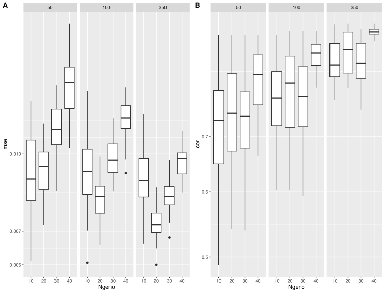
To establish that a combined relationship can be inferred from realizations of its parts, we have conducted the following simulation study: In each round of the simulation, the true parameter value of the genomic relationship matrix was generated as where were independently generated as with a realization from the uniform distribution over was then adjusted by dividing it with the mean value of its diagonal elements. This parameter was taken as the covariance parameter of a Wishart distribution with degrees of freedom 300 and samples from this distribution are generated. After that, each of the realized relationship matrices was made partial by leaving a random sample of 10 to 40 (this number was also selected from the discrete uniform distribution for integers 10 to 40) genotypes in it. These partial kernel matrices were combined using the Wishart EM-Algorithm iterated for 50 rounds (each round cycles through the partial relationship matrices in random order). The resultant combined relationship matrix was compared with the corresponding parts of the parameter 333In certain instances, the union of the genotypes in the parts did not recover all of the genotypes, therefore this calculation was based on the recovered part of the full genomic relationship matrix by calculating the mean squared error between the upper diagonal elements of these matrices. This experiment was replicated 10 times for each value of and
The results of this simulation study are summarized in Figure S1. For each covariance size, the MSE’s decreased as the number of incomplete samples increased. On the other hand, as the size of the covariance matrix increased the MSEs increased.
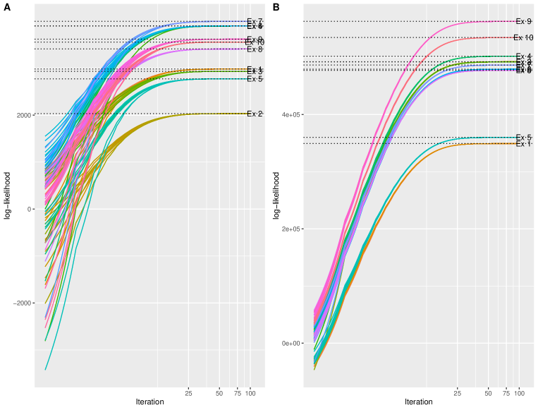
Supplementary Example 2- Simulation study: Likelihood Convergence
The Wishart EM-Algorithm maximizes the likelihood function for a random sample of incomplete observations from a Wishart distribution. The derivation of this feature is given in the Supplementary. In this example, we explore the convergence of the algorithm for several instances starting from several different initial estimates.
The example is composed of 10 experiments each of which starts with a slightly different assumed Wishart covariance parameter444 where for are i.i.d. uniform between 0 and 1.. For each true assumed covariance matrix, we have generated 10 partial samples including between and genotypes (random at discrete uniform from to ) each using the Wishart distribution. the total number of genotypes in the assumed relationship matrix was taken to be or Corresponding to this two matrix sizes the and are taken as 10 and 25 or 100 and 250. These 10 matrices are combined using the Wishart EM-Algorithm 10 different times each times using a slightly different initial estimate of the covariance parameter555 where for are i.i.d. uniform between 0 and 1. . We record the path of the log-likelihood function for all these examples.
At each instance of the parameter and a particular sample, the likelihood functions converged to the same point (See Figure S2). We have not observed any abnormalities in convergence according to these graphs.
Heatmap for 95 wheat traits
Phenotypic network for 186 traits based on phenotypic correlations (Wheat, Barley, and Oat Phenotypic Trials from Triticale Toolbox)
| name | label | name | label | name | label | name | label | name | label |
| 50 seed weight | 50_sw | Cd | Cd | grain fill duration | grfd | Normalized Difference Vegetation Index | NDVI | stripe rust reaction type | srrt |
| aboveground biomass | ab_g_bm | Co | Co | grain hardness | grnh | Normalized water index 3 | Nwi3 | stripe rust reaction type T1 | srrtT1 |
| alpha amylase | alph_am | crown rust infection response | crir | grain number | grnn | P | P | stripe rust reaction type T2 | srrtT2 |
| alpha-tocopherol | alph_tcp | crown rust severity | crs | grain number per spikelet | gnps | peduncle length | pdnl | stripe rust reaction type T3 | srrtT3 |
| alpha-tocotrienol | alph_tct | Cu | Cu | grain protein | grnp | plant height | plnh | stripe rust severity | strrs |
| amylose content | amylose | days to flag leaf senescence | dtfls | grain weight | grnwt | plot shattering | plts | stripe rust severity T1 | srsT1 |
| As | As | days to heading | d_t_h | grain weight per head | gwph | plump grain | plmg | stripe rust severity T3 | srsT3 |
| avenanthramide 2c | aven2c | days to heading (fall planting) | d_t_h_fp | grain width | grnwd | polyphenol oxidase activity | ploa | test weight | tstw |
| avenanthramide 2f | aven2f | delta-tocopherol | dlt-tcp | grain yield | grny | powdery mildew (0-9) | pm | thin grains | thng |
| avenanthramide 2p | aven2p | delta-tocotrienol | dlt-tct | grain yield (main tillers) | grny_mt | powdery mildew incidence | pwmi | thousand kernel weight | thkw |
| avenanthramide 5p | aven5p | diastatic power | dstp | harvest index | hrvi | powdery mildew reaction type | pwmrt | tillers per plant Max | tppM |
| avenanthramide total | avenT | DON | DON | heading date | hdn_dt | productive tillers per plant | ptpp | tillers per plant T2 | tppT2 |
| awn type | awn_type | Fe | Fe | heading date (Julian) | hdn_dt_J | residual beta-glucanase | r_bt-g | tillers per plant T3 | tppT3 |
| bacterial leaf streak | bac_lf_str | fertile spikelets per head | fsph | K | K | S | S | tillers per plant T4 | tppT4 |
| basal aborted spikelets per head | basph | FHB Incidence | FHB_I | kernel weight | krnw | seeds per head | sdph | tillers per plant T5 | tppT5 |
| beta glucan | bt_gl | FHB Severity | FHB_S | kernels per spike | krps | single kernel weight | snkw | tillers per plant T6 | tppT6 |
| beta glucan dwb | bt_gl_dwb | flag leaf angle | fla | leaf chlorophyll content | lfcc | soluble protein/ total protein | sptp | tillers per plant T7 | tppT7 |
| beta-glucanase activity | bt_gl_a | flag leaf angle T1 | flaT1 | leaf rust (0-9) | lr | spike angle | spka | tocol total | tclt |
| beta-glucanase thermostability | bt_gl_t | flag leaf chlorophyll content | flcc | leaf rust reaction type | lrrt | spike density | spkd | tocopherol alpha | tcpa |
| beta-tocopherol | bt-tcp | flag leaf chlorophyll content T1 | flccT1 | leaf rust response | lfrr | spike exsertion | spke | tocopherol beta | tcpb |
| beta-tocotrienol | bt-tct | flag leaf chlorophyll content T2 | flccT2 | leaf rust severity | lfrs | spike length | spkl | tocopherol delta | tcpd |
| biomass at maturity | bm_am | flag leaf length | fll | Li | Li | spike number | spkn | tocopherol gamma | tcpg |
| breeders grain protein | br_gp | flag leaf stay-green period | flsgp | lodging | ldgn | spikelets per head | spph | tocotrienol alpha | tcta |
| breeders plump grain | br_pg | flag leaf width | flw | lodging degree | ldgd | spikelets per panicle | sppp | tocotrienol beta | tctb |
| Ca | Ca | flowering date | flw_d | lodging incidence | ldgi | spikes per area | sppa | tocotrienol delta | tctd |
| canopy senescence score T1 | cssT1 | forage protein | frg_p | lodging severity | ldgs | spot blotch severity | spbs | tocotrienol gamma | tctg |
| canopy senescence score T2 | cssT2 | forage yield | frg_y | malt beta-glucan | mlt_b_g | stem diameter | stmd | total tocol | ttlt |
| canopy senescence score T3 | cssT3 | free amino nitrogen | fan | malt extract | mlt_e | stem length | stml | waxiness | wxns |
| canopy senescence score T4 | cssT4 | freeze injury | frzi | malt protein | mlt_p | stem rust coefficient of infection | srcoi | whole grain protein | wh_gp |
| canopy senescence score T5 | cssT5 | gamma-tocopherol | gmm-tcp | maturity date | mtr_dt | stem rust infection response | srir | winter hardiness | wnt_hrds |
| canopy senescence score T6 | cssT6 | gamma-tocopherol + beta-tocotrienol | gt+bt | maturity date (physiological) | mtr_phy | stem rust severity | stmrs | wort clarity | wrt_clrt |
| canopy senescence score T7 | cssT7 | gamma-tocotrienol | gmm-tct | Mg | Mg | stem solidness | stms | wort color | wrt_clr |
| canopy temperature (grain fill) | ct_gf | glossy sheath | glssysh | Mn | Mn | sterile spikelets per head | ssph | wort protein | wrt_p |
| canopy temperature depression (flowering) | ctd_fl | glossy spike | glssysp | Mo | Mo | straw breakage | strb | WSBMV reaction type | WSBMV_rt |
| canopy temperature depression (grain fill) | ctd_gf | glume pubescence | glmp | Ni | Ni | stripe rust infection type (0-9) | NDVI | Zn | Zn |
6.2 Supplementary Figures