ClusterFit: Improving Generalization of Visual Representations

Abstract

Pre-training convolutional neural networks with weakly-supervised and self-supervised strategies is becoming increasingly popular for several computer vision tasks. However, due to the lack of strong discriminative signals, these learned representations may overfit to the pre-training objective (e.g., hashtag prediction) and not generalize well to downstream tasks. In this work, we present a simple strategy - ClusterFit (CF) to improve the robustness of the visual representations learned during pre-training. Given a dataset, we (a) cluster its features extracted from a pre-trained network using k-means and (b) re-train a new network from scratch on this dataset using cluster assignments as pseudo-labels. We empirically show that clustering helps reduce the pre-training task-specific information from the extracted features thereby minimizing overfitting to the same. Our approach is extensible to different pre-training frameworks – weak- and self-supervised, modalities – images and videos, and pre-training tasks – object and action classification. Through extensive transfer learning experiments on $11$ different target datasets of varied vocabularies and granularities, we show that CF significantly improves the representation quality compared to the state-of-the-art large-scale (millions / billions) weakly-supervised image and video models and self-supervised image models.

1 Introduction

Weak and self-supervised pre-training approaches offer scalability by exploiting free annotation. But there is no free lunch – these methods often first optimize a proxy objective function, for example, predicting image hashtags [31] or color from grayscale images [34, 63]. Similar to supervised pre-training, the underlying assumption (hope) is that this proxy objective function is fairly well aligned with the subsequent transfer tasks, thus optimizing this function could potentially yield suitable pre-trained visual representations. While this assumption holds mostly true in case of fully-supervised pre-training, it may not extend to weak and self-supervision. In the latter pre-training cases, the lack of strong discriminative signals may result in an undesirable scenario where the visual representations overfit to the idiosyncrasies of the pre-training task and dataset instead, thereby rendering them unsuitable for transfer tasks. For instance, it was noted in [38, 51, 20] that factors such as label noise, polysemy (apple the fruit vs. Apple Inc.), linguistic ambiguity, lack of ‘visual’ness of tags (e.g. #love) significantly hampered the pre-training proxy objective from being well-aligned with the transfer tasks. Further, the authors of [64, 22] studied multiple self-supervised methods and observed that, compared to earlier layers, features from the last layer are more “aligned” with the proxy objective, and thus generalize poorly to target tasks.

In this work, we ask a simple question – is there a way to avoid such overfitting to the proxy objective during weak- and self-supervised pre-training? Can we overcome the ‘artifacts’ of proxy objectives so that the representation is generic and transferable? Our key insight is that smoothing the feature space learned via proxy objectives should help us remove these artifacts and avoid overfitting to the the proxy objective. But how do we smoothen the feature space? Should it be done while optimizing the proxy objective or in a post-hoc manner?

Pre-training method (${\color[rgb]{0.5,0.0,0.5}\mathrm{N_{pre}}}$)	$\mathbf{\Delta}$ of CF (${\color[rgb]{0.0,0.5,0.0}\mathrm{N_{cf}}}$) on transfer
Fully-supervised Images section 3.2, fig. 3b	+2.1% on ImageNet-9K [10]
ResNet-50, ImageNet-1K, 1K labels
Weakly-supervised Images section 4.1.1, table 4	+4.6% on ImageNet-9K [10]
ResNet-50, 1B Images, 1.5K hashtags [38]	+5.8% on iNaturalist [55]
Weakly-supervised Videos section 4.1.2, table 5	+3.2% on Kinetics [59]
R(2+1)D-34, 19M videos, 438 hashtags [20]	+4.3% on Sports1M [32]
Self-supervised Images section 4.2, Tables 6, 8	+7-9% on ImageNet-1K [47]
ResNet-50, 1M images	+3-7% mAP on VOC07 [15]
Jigsaw [42] and RotNet [21], Multi-task (appendix E)	+3-5% on Places205 [65]

Table 1: A summary of results: We show that ClusterFit (CF) can be applied to a variety of different pre-training methods, modalities, and architectures. We report absolute gains in top-1 accuracy (except for VOC07 where we report mAP). In each setting, CF provides improvements with the same model architecture and without additional data or supervision.

To this end, we propose a surprisingly simple yet effective framework called ClusterFit (CF). Specifically, given a pre-trained network trained using a proxy objective and a new dataset, we first use the learned feature space to cluster that dataset. Next, we train a new network from scratch on this new dataset using the cluster memberships as pseudo labels (fig. 1). We demonstrate that clustering of the features helps retain only the essential invariances in them and eliminates proxy objective’s artifacts (essentially smoothing the feature space). Re-training on the cluster memberships yields a visually coherent pre-training feature space for downstream tasks. Our approach of feature space smoothing is guided through unsupervised k-means clustering, making it scalable to millions (billions) of videos and images in both weak- and self-supervised pre-training frameworks.

We take inspiration from recent work in self-supervised learning which aims to learn a smooth visual feature space via clustering and trains representations on the clusters as classes [6, 7, 44]. While [6, 7] use clustering as the training objective itself, in our work, we investigate the value of post-hoc smoothing. ClusterFit can also be viewed as a variant of knowledge distillation [28] that distills via ‘lossy’ clustering, as opposed to the standard setup of using soft targets in original label space.

ClusterFit demonstrates significant performance gains on a total of $11$ public, challenging image and video benchmark datasets. As summarized in table 1, our approach, while extremely simple, consistently improves performance across different pre-training methods, input modalities, network architectures, and benchmark datasets.

2 Related Work

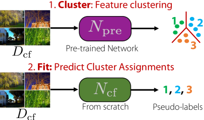
Figure 1: ClusterFit (CF): We start with a pre-trained network (${\color[rgb]{0.5,0.0,0.5}\mathrm{N_{pre}}}$) that is trained on some pre-training task (not shown). We use this network to extract features and cluster a new dataset ${\color[rgb]{0.0,0.5,0.0}\mathrm{D_{cf}}}$ using k-means clustering. We show that training a new network ${\color[rgb]{0.0,0.5,0.0}\mathrm{N_{cf}}}$ from scratch on these cluster assignments as labels results in a more transferable feature representation.

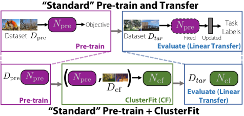
Figure 2: Full ClusterFit pipeline: A typical transfer learning framework involves two stages: pre-training followed by transfer learning. ClusterFit introduces a step between these stages. We evaluate all representations by training a linear classifier on fixed ConvNet weights.

Weakly Supervised Learning: Training ConvNets on very large, weakly supervised images by defining the proxy tasks using the associated meta-data [38, 51, 24, 31, 36, 11, 52, 48, 53, 56, 20] has shown tremendous benefits. Proxy tasks include hashtags predictions [38, 56, 11, 24, 20], GPS [26, 58], search queries prediction [51], and word or n-grams predictions [31, 36]. Our approach builds upon these works and shows that even better representations can be trained by leveraging the features from such pre-training frameworks for clustering to mitigate the effect of noise. Yalniz et al. [62] propose a target task specific noise removal framework by ranking images for each class by their softmax values and retaining only top-$K$ images for re-training. However, their method is specific to a particular target task and discards most of the data during re-training. By contrast, our approach does not adhere to a particular target task and leverages all the data, since, they may contain complementary visual information beyond hashtags.

Self-Supervised Learning: Self-supervised approaches typically learn a feature representation by defining a ‘pre-text’ task on the visual domain. These pre-text tasks can either be domain agnostic [5, 45, 60, 29, 6, 61] or exploit domain-specific information like spatial structure in images [13, 42, 43, 44, 21], color [12, 34, 35, 64, 63], illumination [14], temporal structure [40, 25, 16, 39, 37] or a co-occurring modality like sound [2, 3, 19, 46, 9]. In this work, we use two diverse image-based self-supervision approaches - Jigsaw [42] and RotNet [21] that have shown competitive performance [22, 7, 33]. Since the difference between pretext tasks and semantic transfer learning tasks is huge, our method shows much larger improvement for self-supervised methods (section 4.2).

Our work builds upon [6, 7], who use clustering and pseudo-labels for self-supervised learning and [44], who distill predictions from different self-supervised models to a common architecture. Compared to [6, 7], ClusterFit does not require any alternate optimization and thus is more stable and computationally efficient. As we show in section 4, this property makes ClusterFit easily scalable to different modalities and large-scale data. Compared to [44], our focus is not distilling information to a common architecture, but instead to remove the pre-training task biases. This makes ClusterFit applicable broadly to any kind of pre-trained models - fully supervised or use noisy supervision (section 3.2), weakly supervised from billions of images or millions of videos (section 4.1), and self-supervised models (section 4.2).

Model Distillation: Model distillation [4, 28, 18, 1] typically involves transferring knowledge from a ‘teacher’ model to a ‘student’ model by training the student on predictions of the teacher in addition to task labels. These methods are designed to transfer knowledge (not contained in the labels) about the task from the teacher to the student network. Since distillation retains more knowledge about the original task, it performs poorly in the case of weak-supervision (section 4.1). Interestingly, the failure of standard knowledge distillation approaches in the context of self-supervised learning has also been shown in  [44].

Dataset	Label Type	# classes	Train/Eval	Metric
Weakly-supervised Images section 4.1.1
ImageNet-1K [47]	multi-class object	1000	1.3M/50K	top-1 acc
ImageNet-9K [10]	multi-class object	9000	10.5M/450K	top-1 acc
Places365 [65]	multi-class scene	365	1.8M/36.5K	top-1 acc
iNaturalist 2018 [55]	multi-class object	8142	438K/24K	top-1 acc
Weakly-supervised Videos section 4.1.2
Kinetics [59]	multi-class action	400	246K/20K	top-1 acc
Sports1M [32]	multi-class action	487	882K/204K	top-1 acc
Something-Something V1 [23]	multi-class action	174	86K/11.5K	top-1 acc
Self-supervised Images section 4.2
VOC07 [15]	multi-label object	20	5K/5K	mAP
ImageNet-1K [47]	multi-class object	1000	1.3M/50K	top-1 acc
Places205 [65]	multi-class scene	205	2.4M/21K	top-1 acc
iNaturalist 2018 [55]	multi-class object	8142	438K/24K	top-1 acc

Table 2: Target tasks for Transfer Learning used for evaluating feature representations.

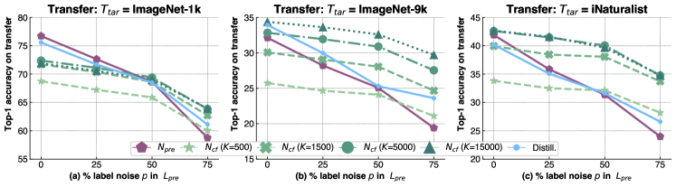
Figure 3: Control Experiment: We inject uniform label noise in the labels ${\color[rgb]{0.5,0.0,0.5}\mathrm{L_{pre}}}$ from ${\color[rgb]{0.5,0.0,0.5}\mathrm{D_{pre}}}\!=$ ImageNet-1K and train a separate ResNet-50 model (${\color[rgb]{0.5,0.0,0.5}\mathrm{N_{pre}}}$) on these noisy labels. We apply ClusterFit on each of these pre-trained models (${\color[rgb]{0.5,0.0,0.5}\mathrm{N_{pre}}}$) and vary the number of clusters $K$ to train ${\color[rgb]{0.0,0.5,0.0}\mathrm{N_{cf}}}$. We then study the transfer learning performance of the representations by training a linear classifier on fixed features from ${\color[rgb]{0.5,0.0,0.5}\mathrm{N_{pre}}}$ or ${\color[rgb]{0.0,0.5,0.0}\mathrm{N_{cf}}}$ on three target tasks - a noise free ImageNet-1K, ImageNet-9K, and iNaturalist. ClusterFit is able to learn more transferable features despite high amounts of label noise in pre-training. For finer-grained target tasks like ImageNet-9K, ClusterFit can even improve a fully supervised ResNet-50 model ($p\!=\!0$).

3 Approach

Our goal is to learn a generalizable feature space for a variety of target tasks that does not overfit to the pre-training proxy objective. We first describe the framework of ClusterFit (CF) in section 3.1. Next, we report a control experiment on the ImageNet-1K dataset that sheds light on how CF combats the ‘bias’ introduced due to the proxy objective (section 3.2).

3.1 ClusterFit Framework

Our method starts with a ConvNet ${\color[rgb]{0.5,0.0,0.5}\mathrm{N_{pre}}}$ that is pre-trained on a dataset ${\color[rgb]{0.5,0.0,0.5}\mathrm{D_{pre}}}$ and labels ${\color[rgb]{0.5,0.0,0.5}\mathrm{L_{pre}}}$. First, we use the penultimate layer of ${\color[rgb]{0.5,0.0,0.5}\mathrm{N_{pre}}}$ to extract features from each datapoint belonging to another dataset ${\color[rgb]{0.0,0.5,0.0}\mathrm{D_{cf}}}$. Next, we cluster these features using k-means into $K$ groups and treat these cluster assignments as the new categorical ‘labels’ (${\color[rgb]{0.0,0.5,0.0}\mathrm{L_{cf}}}$) for ${\color[rgb]{0.0,0.5,0.0}\mathrm{D_{cf}}}$. Finally, we fit a different network ${\color[rgb]{0.0,0.5,0.0}\mathrm{N_{cf}}}$ (initialized from scratch) on ${\color[rgb]{0.0,0.5,0.0}\mathrm{D_{cf}}}$ that minimizes a cross-entropy objective on ${\color[rgb]{0.0,0.5,0.0}\mathrm{L_{cf}}}$. We illustrate these steps in Figure 1. We highlight that re-learning ${\color[rgb]{0.0,0.5,0.0}\mathrm{N_{cf}}}$ from scratch on ${\color[rgb]{0.0,0.5,0.0}\mathrm{D_{cf}}}$ is completely unsupervised and thus allows leveraging large-scale datasets.

Intuition: We hypothesize that ClusterFit (CF) leverages the underlying visual smoothness in the feature space to create visually coherent clusters. We believe that “cluster” followed by “fit” weakens the underlying pre-training objective-specific bias. One may view ClusterFit from an information bottleneck [54] perspective wherein the ‘lossy’ clustering step introduces a bottleneck and removes any pre-training proxy objective bias.

How to evaluate CF? As in prior efforts [38, 22, 20], we use transfer learning performance on downstream tasks to understand whether CF improves generalization of the feature representations. Specifically, to evaluate ${\color[rgb]{0.5,0.0,0.5}\mathrm{N_{pre}}}$ and ${\color[rgb]{0.0,0.5,0.0}\mathrm{N_{cf}}}$, we train linear classifiers on fixed feature representations from the networks on the downstream task and report final performance on held-out data (see table 2). Figure 2 illustrates ClusterFit’s setup. We stress that ClusterFit is simple to implement and makes minimal assumptions about input modalities, architectures etc. but provides a powerful way to improve the generalization of the feature space. We explore various design choices ClusterFit offers such as relative properties of ${\color[rgb]{0.5,0.0,0.5}\mathrm{N_{pre}}}$, ${\color[rgb]{0.0,0.5,0.0}\mathrm{N_{cf}}}$, ${\color[rgb]{0.5,0.0,0.5}\mathrm{D_{pre}}}$, and ${\color[rgb]{0.0,0.5,0.0}\mathrm{D_{cf}}}$ in section 5.

3.2 Control Experiment using Synthetic Noise

Here, our goal is to study the extent of generalization of features learned from a ‘proxy’ pre-training objective in a controlled setup. We start with a supervised pre-training dataset ImageNet-1K [47], and add synthetic label noise to it. Our motive behind this setup is to intentionally misalign the pre-training objective with downstream tasks. We acknowledge that the synthetic noise simulated in this experiment is an over simplification of the complex noise present in real world data. Nevertheless, it provides several key insights into ClusterFit as we show next.

Control Experiment Setup: To isolate the effect of CF, in this experiment, we fix ${\color[rgb]{0.5,0.0,0.5}\mathrm{D_{pre}}}\!=\!{\color[rgb]{0.0,0.5,0.0}\mathrm{D_{cf}}}\!=$ ImageNet-1K and the network architectures ${\color[rgb]{0.5,0.0,0.5}\mathrm{N_{pre}}}$ and ${\color[rgb]{0.0,0.5,0.0}\mathrm{N_{cf}}}$ to ResNet-50 [27]. We start by adding varying amounts ($p\%$) of uniform random label noise to ${\color[rgb]{0.5,0.0,0.5}\mathrm{D_{pre}}}$. Next, we train a separate ${\color[rgb]{0.5,0.0,0.5}\mathrm{N_{pre}}}$ for each fraction $p$ of the noisy labels. We then apply CF (with different values of $K$ in k-means) to each ${\color[rgb]{0.5,0.0,0.5}\mathrm{N_{pre}}}$ to obtain a corresponding ${\color[rgb]{0.0,0.5,0.0}\mathrm{N_{cf}}}$. Finally, we evaluate the representations by training linear classifiers on fixed res5 features on three target image classification datasets - ImageNet-1K, ImageNet-9K, and iNaturalist. We use model distillation [28] as a baseline to better understand the behavior of ClusterFit.

Our motivation behind this setup is the following: when $p\!=\!0$, ${\color[rgb]{0.5,0.0,0.5}\mathrm{N_{pre}}}$ denotes the true, noise-free supervised task; as $p$ increases, the proxy objective becomes a poorer approximation of the original pre-training objective and allows us to closely inspect ClusterFit.

Results and Observations: We report the transfer learning performance of ${\color[rgb]{0.5,0.0,0.5}\mathrm{N_{pre}}}$ (i.e., before CF) and ${\color[rgb]{0.0,0.5,0.0}\mathrm{N_{cf}}}$ (i.e., after CF) in fig. 3 for different values of label noise $p$. Let us first consider $p=0$, i.e., a setting without any label noise. In this case, ${\color[rgb]{0.5,0.0,0.5}\mathrm{N_{pre}}}$ is trained on clean labels. On the target dataset ImageNet-1K, ${\color[rgb]{0.5,0.0,0.5}\mathrm{N_{pre}}}$ performs significantly better than ${\color[rgb]{0.0,0.5,0.0}\mathrm{N_{cf}}}$ for all values of $K$ (Fig. 3 (a)). This is expected, since when ${\color[rgb]{0.5,0.0,0.5}\mathrm{D_{pre}}}\!=\!{\color[rgb]{0.0,0.3,0.8}\mathrm{D_{tar}}}=$ ImageNet-1K, the pre-training and transfer tasks are exactly aligned. However, ${\color[rgb]{0.0,0.5,0.0}\mathrm{N_{cf}}}$ performs comparably or better than ${\color[rgb]{0.5,0.0,0.5}\mathrm{N_{pre}}}$ for other target da - ImageNet-9K and iNaturalist at higher values of $K$. This suggests that CF can improve even fully-supervised representations for more fine-grained downstream tasks. We note that model distillation also provides an improvement over ${\color[rgb]{0.5,0.0,0.5}\mathrm{N_{pre}}}$ on ImageNet-9K but is worse on iNaturalist.

Let us now consider scenarios where $p>0$. Figure 3 indicates that increased label noise ($p$) in ${\color[rgb]{0.5,0.0,0.5}\mathrm{D_{pre}}}$ translates to poor performance across all three target tasks. We highlight that the drop in the performance is more drastic for ${\color[rgb]{0.5,0.0,0.5}\mathrm{N_{pre}}}$ (i.e., before CF), than for ${\color[rgb]{0.0,0.5,0.0}\mathrm{N_{cf}}}$ (i.e., after CF). More importantly, the performance gap between ${\color[rgb]{0.0,0.5,0.0}\mathrm{N_{cf}}}$ and ${\color[rgb]{0.5,0.0,0.5}\mathrm{N_{pre}}}$ continues to increase with $p$. From Fig. 3 (b) and (c), we observe that ${\color[rgb]{0.0,0.5,0.0}\mathrm{N_{cf}}}$ consistently outperforms ${\color[rgb]{0.5,0.0,0.5}\mathrm{N_{pre}}}$ on two target tasks ImageNet-9K and iNaturalist. Notably, for ${\color[rgb]{0.0,0.3,0.8}\mathrm{D_{tar}}}\!=$ ImageNet-1K (fig. 3 (a)), when $p\geq 50$, ${\color[rgb]{0.0,0.5,0.0}\mathrm{N_{cf}}}$ outperform ${\color[rgb]{0.5,0.0,0.5}\mathrm{N_{pre}}}$, which is pre-trained on noisy ImageNet-1K. Model distillation provides some gains over ${\color[rgb]{0.5,0.0,0.5}\mathrm{N_{pre}}}$ but is consistently outperformed by ClusterFit.

These results suggest that as $p$ increases, the proxy objective gets further away from the ‘true’ pre-training objective, and makes features from ${\color[rgb]{0.5,0.0,0.5}\mathrm{N_{pre}}}$ less transferable. In those very cases, CF captures useful visual invariances in the feature representations, thereby providing more noise-resilient pseudo-labels for learning transferable representations. Finally, we also note that larger number of clusters $K$ generally leads to better transfer learning performance. The gains are larger for more challenging and fine-grained datasets like ImageNet-9K and iNaturalist. We study the effect of this hyper-parameter $K$ in section 5.

4 Experiments

We now examine the broad applicability of ClusterFit in three different pre-training scenarios for ${\color[rgb]{0.5,0.0,0.5}\mathrm{N_{pre}}}$: (a) weakly-supervised pre-training for images  (section 4.1.1), (b) weakly-supervised pre-training for videos (section 4.1.2), and (c) self-supervised pre-training for images (section 4.2).

Common CF Setting: Throughout this section, we set ${\color[rgb]{0.5,0.0,0.5}\mathrm{D_{pre}}}$ $=$ ${\color[rgb]{0.0,0.5,0.0}\mathrm{D_{cf}}}$ and ${\color[rgb]{0.5,0.0,0.5}\mathrm{N_{pre}}}$ $=$ ${\color[rgb]{0.0,0.5,0.0}\mathrm{N_{cf}}}$ (architecture-wise). We train ${\color[rgb]{0.5,0.0,0.5}\mathrm{N_{pre}}}$ on ${\color[rgb]{0.5,0.0,0.5}\mathrm{D_{pre}}}$, ${\color[rgb]{0.0,0.5,0.0}\mathrm{N_{cf}}}$ on ${\color[rgb]{0.0,0.5,0.0}\mathrm{D_{cf}}}$ for equal number of epochs.  table 3 summarizes these settings. By keeping the data, architecture, and training schedule constant, we hope to measure the difference in performance between ${\color[rgb]{0.0,0.5,0.0}\mathrm{N_{cf}}}$ and ${\color[rgb]{0.5,0.0,0.5}\mathrm{N_{pre}}}$ solely due to ClusterFit.

Evaluation: As mentioned in section 3.1, we evaluate ClusterFit via transfer learning on target tasks. Specifically, we train linear classifiers on the fixed features obtained from the penultimate layer of ${\color[rgb]{0.5,0.0,0.5}\mathrm{N_{pre}}}$ or ${\color[rgb]{0.0,0.5,0.0}\mathrm{N_{cf}}}$ on target datasets. The transfer learning tasks are summarized in table 2.

Baselines: We use the following baselines:

• $\color[rgb]{0.5,0.0,0.5}\mathbf{N_{pre}}$: We use features from ${\color[rgb]{0.5,0.0,0.5}\mathrm{N_{pre}}}$ for transfer learning. Since ClusterFit (CF) is applied on ${\color[rgb]{0.5,0.0,0.5}\mathrm{N_{pre}}}$ to get ${\color[rgb]{0.0,0.5,0.0}\mathrm{N_{cf}}}$, this baseline serves to show improvements through CF.

• Distillation: To empirically understand the importance of the clustering step in CF, we compare with model distillation [28]. Unlike CF, distillation transfers knowledge from ${\color[rgb]{0.5,0.0,0.5}\mathrm{N_{pre}}}$ without clustering, thus retaining more information about the learned features. We train a distilled model using a weighted average of $2$ loss functions: (a) cross-entropy with soft targets computed using ${\color[rgb]{0.5,0.0,0.5}\mathrm{N_{pre}}}$ and temperature $T$ and (b) cross-entropy with image/video labels in weakly-supervised setup. We also experimented with training a network to directly regress the features from ${\color[rgb]{0.5,0.0,0.5}\mathrm{N_{pre}}}$ but found consistently worse results.

• Prototype: ClusterFit uses unsupervised k-means to create pseudo-labels. To understand the effect of this unsupervised step, we add a baseline that uses semantic information during clustering. Under this prototype alignment [49] baseline, unlike random cluster initialization as done in k-means, we use label information in ${\color[rgb]{0.0,0.5,0.0}\mathrm{D_{cf}}}$ to initialize cluster centers. Specifically, we first set $K$ equal to the number of ‘classes’ in ${\color[rgb]{0.0,0.5,0.0}\mathrm{D_{cf}}}$. Here, each cluster corresponds to a ‘prototype’ of that class. We then compute $K$ prototypes by averaging image embeddings of all images belonging to each class. Finally, pseudo-labels are assigned to each data point by finding its nearest ‘prototype’ cluster center. Since this method uses explicit label information present in ${\color[rgb]{0.0,0.5,0.0}\mathrm{D_{cf}}}$, it requires more ‘supervision’ than ClusterFit. We also note that this baseline is not applicable to self-supervised methods (suppl. material).

• Longer pre-training: Since ${\color[rgb]{0.0,0.5,0.0}\mathrm{N_{cf}}}$ is trained for the same number of epochs as ${\color[rgb]{0.5,0.0,0.5}\mathrm{N_{pre}}}$, we also compare against a network trained on the pre-train task for $2\times$ longer (denoted by ${\color[rgb]{0.5,0.0,0.5}\mathrm{N_{pre}}}2\times$). Specifically, ${\color[rgb]{0.5,0.0,0.5}\mathrm{N_{pre}}}2\times$ is trained for a combined number of epochs as ${\color[rgb]{0.5,0.0,0.5}\mathrm{N_{pre}}}$ and ${\color[rgb]{0.0,0.5,0.0}\mathrm{N_{cf}}}$. By comparing ${\color[rgb]{0.0,0.5,0.0}\mathrm{N_{cf}}}$ against this baseline, we hope to isolate improvements due to longer pre-training.

Pre-training method	${\color[rgb]{0.5,0.0,0.5}\mathrm{D_{pre}}}\!=\!{\color[rgb]{0.0,0.5,0.0}\mathrm{D_{cf}}}$	Arch. of ${\color[rgb]{0.5,0.0,0.5}\mathrm{N_{pre}}}$ & ${\color[rgb]{0.0,0.5,0.0}\mathrm{N_{cf}}}$
Weakly-Supervised Images section 4.1.1	IG-ImageNet-1B	ResNet-50
Weakly-Supervised Videos section 4.1.2	IG-Verb-19M	R(2+1)D-34
Self-supervised Images section 4.2	ImageNet-1k	ResNet-50

Table 3: Data and model architectures used in section 4: weakly supervised videos, weakly supervised images, and self supervised images. In each setting, we train ${\color[rgb]{0.5,0.0,0.5}\mathrm{N_{pre}}}$ and ${\color[rgb]{0.0,0.5,0.0}\mathrm{N_{cf}}}$ for equal number of epochs.

4.1 Weakly-supervised pre-training

In this section, we study weakly-supervised pre-training on noisy web images and videos. These approaches predict the noisy hashtags associated with images/videos and thus minimize a proxy objective during pre-training.

${\color[rgb]{0.0,0.3,0.8}\mathrm{D_{tar}}}$	${\color[rgb]{0.5,0.0,0.5}\mathrm{N_{pre}}}$	${\color[rgb]{0.5,0.0,0.5}\mathrm{N_{pre}}}2\times$	Distill.	Prototype	CF (${\color[rgb]{0.0,0.5,0.0}\mathrm{N_{cf}}}$), $K$ $\rightarrow$
					$1.5k$	$3.75k$	$7.5k$	$15k$	$30k$
ImageNet-1K	78.0	78.8	73.8	76.9	75.3	76.1	76.5	76.5	76.2
ImageNet-9K	32.9	34.1	29.1	35.1	33.5	35.4	36.4	37.1	37.5
Places365	51.2	51.2	49.9	51.9	52.0	52.1	52.4	52.6	52.1
iNaturalist	43.9	45.3	35.9	49.0	43.8	46.4	47.9	49.7	49.5

Table 4: Weakly-supervised Images: Top-1 accuracy for various transfer learning datasets with ${\color[rgb]{0.5,0.0,0.5}\mathrm{D_{pre}}}$ = ${\color[rgb]{0.0,0.5,0.0}\mathrm{D_{cf}}}$ = IG-ImageNet-1B and the same architecture (ResNet-50) for ${\color[rgb]{0.5,0.0,0.5}\mathrm{N_{pre}}}$ and ${\color[rgb]{0.0,0.5,0.0}\mathrm{N_{cf}}}$.

4.1.1 Weakly-supervised image pre-training

Data and Model: As in [38], we collect IG-ImageNet-1B dataset of 1B public images associated with hashtags from a social media website. To construct this dataset, we consider images tagged with at least one hashtag that maps to any of the ImageNet-1K synsets. The architecture of ${\color[rgb]{0.5,0.0,0.5}\mathrm{N_{pre}}}$ and ${\color[rgb]{0.0,0.5,0.0}\mathrm{N_{cf}}}$ network is fixed to a ResNet-50 [27], while ${\color[rgb]{0.5,0.0,0.5}\mathrm{D_{pre}}}$ $=$ ${\color[rgb]{0.0,0.5,0.0}\mathrm{D_{cf}}}$ $=$ IG-ImageNet-1B.

ClusterFit Details: We extract features from the $2048$ dimensional res5 layer from ${\color[rgb]{0.5,0.0,0.5}\mathrm{N_{pre}}}$ for clustering. ${\color[rgb]{0.0,0.5,0.0}\mathrm{N_{cf}}}$ is trained from scratch on ${\color[rgb]{0.0,0.5,0.0}\mathrm{D_{cf}}}$ $=$ IG-ImageNet-1B on the cluster assignments as pseudo-labels. Details on the hyper parameters during pre-training and ClusterFit are provided in the supplementary material. We report results in table 4, which we discuss next.

Effect of longer pre-training: ${\color[rgb]{0.5,0.0,0.5}\mathrm{N_{pre}}}$ pre-trained on ${\color[rgb]{0.5,0.0,0.5}\mathrm{D_{pre}}}$ $=$IG-ImageNet-1B already exhibits very strong performance on all target datasets. By construction, the label space of the target dataset ImageNet-1K matches with that of ${\color[rgb]{0.5,0.0,0.5}\mathrm{D_{pre}}}$. As noted in [38], this translates to ${\color[rgb]{0.5,0.0,0.5}\mathrm{N_{pre}}}$ yielding an impressive top-1 accuracy of 78% on ImageNet-1K. Features from longer pre-training (${\color[rgb]{0.5,0.0,0.5}\mathrm{N_{pre}}}2\times$) show improvements on ImageNet-1K, ImageNet-9K, and iNaturalist but not on Places365. As noted in [31, 38], Places365 is not well-aligned with ImageNet-1K (and by extension with IG-ImageNet-1B). Thus, (longer) pre-training yields no benefit. By contrast, the target dataset ImageNet-9K is well-aligned with ${\color[rgb]{0.5,0.0,0.5}\mathrm{D_{pre}}}$ $=$ IG-ImageNet-1B, thus achieving improvements from longer pre-training.

Comparison with Model Distillation: Training a student network via distillation, i.e., soft targets provided by the teacher (${\color[rgb]{0.5,0.0,0.5}\mathrm{N_{pre}}}$) and hashtags, performs worse than ${\color[rgb]{0.5,0.0,0.5}\mathrm{N_{pre}}}$ itself. In our case, the student and teacher network are of the same capacity (ResNet-50). We believe that the noisy label setting combined with the same capacity student and teacher networks are not ideal for model distillation.

Comparison with Prototype: Except on ImageNet-1K, the prototype baseline shows improvement over both ${\color[rgb]{0.5,0.0,0.5}\mathrm{N_{pre}}}$ and ${\color[rgb]{0.5,0.0,0.5}\mathrm{N_{pre}}}2\times$. This shows that pseudo-labels derived based on label information can provide a better training objective than hashtags used for pre-training ${\color[rgb]{0.5,0.0,0.5}\mathrm{N_{pre}}}$. However, similar to CF, prototype shows a reduction in performance on ImageNet-1K which we explain next.

Gains of ClusterFit: ${\color[rgb]{0.0,0.5,0.0}\mathrm{N_{cf}}}$ achieves substantial gains over the strong ${\color[rgb]{0.5,0.0,0.5}\mathrm{N_{pre}}}$ model especially on fine-grained datasets like ImageNet-9K (4.6 points) and iNaturalist (5.8 points), at higher values of $K$. This may be because ${\color[rgb]{0.0,0.5,0.0}\mathrm{N_{cf}}}$ captures a more diverse and finer-grained visual feature space that benefits fine-grained transfer tasks. We observe a small decrease in the performance on ImageNet-1K (1.5 points) which can be attributed again to the hand-crafted label alignment of the IG-ImageNet-1B with ImageNet-1K. This result is inline with observations from [38]. We believe the performance decrease of ‘prototype’ on ImageNet-1K is also due to this reason. ${\color[rgb]{0.0,0.5,0.0}\mathrm{N_{cf}}}$ shows improved performance than ‘prototype,’ yet does not use any additional supervision while generating pseudo-labels. Finally, we note that finding an optimal number of clusters $K$ for each transfer learning task is procedurally easier than finding a pre-training task (or label space) that aligns with the target task.

${\color[rgb]{0.0,0.3,0.8}\mathrm{T_{tar}}}$	${\color[rgb]{0.5,0.0,0.5}\mathrm{N_{pre}}}$	${\color[rgb]{0.5,0.0,0.5}\mathrm{N_{pre}}}2\times$	Distill.	Prototype	CF (${\color[rgb]{0.0,0.5,0.0}\mathrm{N_{cf}}}$), $K$ $\rightarrow$
					$400$	$800$	$1600$	$3200$	$6400$
Kinetics	68.8	69.2	63.6	70.3	70.1	71.2	71.2	71.5	72.0
Sports1M	52.9	53.1	48.4	55.1	55.8	56.6	57.1	57.2	57.2
Sth-Sth V1	16.9	16.4	15.6	20.3	20.2	20.0	20.6	19.3	19.7

Table 5: Weakly-supervised videos: Top-1 accuracy for various transfer learning datasets with ${\color[rgb]{0.5,0.0,0.5}\mathrm{D_{pre}}}$ = ${\color[rgb]{0.0,0.5,0.0}\mathrm{D_{cf}}}$ = IG-Verb-19M and the same architecture (R(2+1)D-34) for ${\color[rgb]{0.5,0.0,0.5}\mathrm{N_{pre}}}$ and ${\color[rgb]{0.0,0.5,0.0}\mathrm{N_{cf}}}$.

4.1.2 Weakly-supervised video pre-training

Data and Model: Following [20], we collect IG-Verb-19M, a dataset of $19M$ public videos with hashtags from a social media website. We consider videos tagged with at least one of the $438$ verbs from Kinetics [59] and VerbNet [57]. We set ${\color[rgb]{0.5,0.0,0.5}\mathrm{D_{pre}}}$ $=$ ${\color[rgb]{0.0,0.5,0.0}\mathrm{D_{cf}}}$ $=$ IG-Verb-19M. We use the clip-based R(2+1)D-34 [8] architecture for ${\color[rgb]{0.5,0.0,0.5}\mathrm{N_{pre}}}$ and ${\color[rgb]{0.0,0.5,0.0}\mathrm{N_{cf}}}$. Each video clip is generated by scaling its shortest edge to $128$ followed by cropping a random patch of size $112\!\times\!112$. We use $32$ consecutive frames per video clip, with temporal jittering applied to the input.

ClusterFit details: We uniformly sample $6$ clips of $32$ consecutive frames per video, extract video features per clip, and average pool them. We use the $512$ dimensional res5 layer from ${\color[rgb]{0.5,0.0,0.5}\mathrm{N_{pre}}}$. We direct the reader to the supplementary material for hyper-parameter details.

Observations: We present the transfer learning results in Table 5. Once again, the baseline ${\color[rgb]{0.5,0.0,0.5}\mathrm{N_{pre}}}$ exhibits strong performance on all target datasets. Longer pretraining (${\color[rgb]{0.5,0.0,0.5}\mathrm{N_{pre}}}2\times$) provides limited benefit on Kinetics and Sports1M, and loses performance compared to ${\color[rgb]{0.5,0.0,0.5}\mathrm{N_{pre}}}$ on Sth-Sth V1. As observed in section 4.1.1, model distillation performs worse than ${\color[rgb]{0.5,0.0,0.5}\mathrm{N_{pre}}}$ on all target datasets.

We observe that CF (${\color[rgb]{0.0,0.5,0.0}\mathrm{N_{cf}}}$) provides significant improvements of $\textbf{3.2 - 4.3}\%$ across all the datasets over ${\color[rgb]{0.5,0.0,0.5}\mathrm{N_{pre}}}$. The optimal number of clusters $K$ vary depending on each dataset, but is typically an order of magnitude higher than the size of the original label space (i.e., $438$ verbs in IG-Verb-19M). For example, performance does not saturate for Kinetics even at $K=6400$. We study the effect of $K$ in section 5.2.

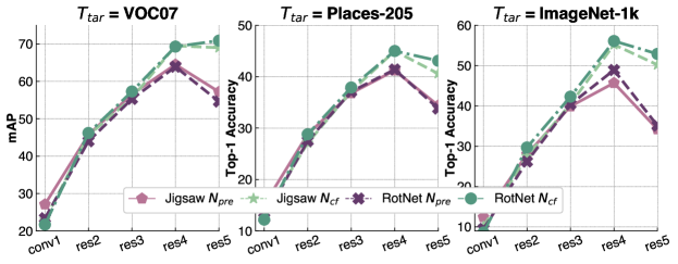
Figure 4: Self-supervised Images (Layerwise): We examine the layer-wise performance of self-supervised models before applying our technique (${\color[rgb]{0.5,0.0,0.5}\mathrm{N_{pre}}}$) and after (${\color[rgb]{0.0,0.5,0.0}\mathrm{N_{cf}}}$). We fix ${\color[rgb]{0.5,0.0,0.5}\mathrm{D_{pre}}}\!=\!{\color[rgb]{0.0,0.5,0.0}\mathrm{D_{cf}}}\!=\$ImageNet-1K (without labels) and use the same architecture (ResNet-50) for ${\color[rgb]{0.5,0.0,0.5}\mathrm{N_{pre}}}$ and ${\color[rgb]{0.0,0.5,0.0}\mathrm{N_{cf}}}$. The last layer (res5) features for ${\color[rgb]{0.5,0.0,0.5}\mathrm{N_{pre}}}$ transfer poorly compared to the lower res4 layer. After CF, ${\color[rgb]{0.0,0.5,0.0}\mathrm{N_{cf}}}$ shows an improved performance for all layers except for conv1 and reduces the gap in performance between res4 and res5.

4.2 Self-Supervised pre-training for Images

We now apply ClusterFit framework to self-supervised methods. We study two popular and diverse self-supervised methods - Jigsaw [42] and RotNet [21]. These methods do not use semantic labels and instead create pre-training labels using a ‘pre-text’ task such as rotation. As mentioned in section 2 and [44], distillation is not a valid baseline for these self-supervised methods (more in supplementary material). Also, as these methods do not use semantic label information, ‘prototype’ is also not a valid baseline.

Data and Model: We fix the network architectures of ${\color[rgb]{0.5,0.0,0.5}\mathrm{N_{pre}}}$ and ${\color[rgb]{0.0,0.5,0.0}\mathrm{N_{cf}}}$ to ResNet-50. We also fix ${\color[rgb]{0.5,0.0,0.5}\mathrm{D_{pre}}}$ $=$ ${\color[rgb]{0.0,0.5,0.0}\mathrm{D_{cf}}}$ = ImageNet-1K to pre-train Jigsaw and RotNet models (${\color[rgb]{0.5,0.0,0.5}\mathrm{N_{pre}}}$). We discard the semantic labels and use only images from both tasks. We use the models released by [22] for Jigsaw and train RotNet models following the approach in [21, 22].

ClusterFit Details: We set $K\!=\!16,000$. ${\color[rgb]{0.0,0.5,0.0}\mathrm{N_{cf}}}$ is trained for the same number of epochs as the pre-trained self-supervised network ${\color[rgb]{0.5,0.0,0.5}\mathrm{N_{pre}}}$. We strictly follow the training hyper parameters and the transfer learning setup outlined in Goyal et al. [22]. We report additional results for different values of $K$ in the supplemental material.

Layer-wise transfer: In fig. 4, we report the transfer learning performance of each layer of ${\color[rgb]{0.5,0.0,0.5}\mathrm{N_{pre}}}$ and compare with ${\color[rgb]{0.0,0.5,0.0}\mathrm{N_{cf}}}$ after applying ClusterFit. We see that for the pre-trained network ${\color[rgb]{0.5,0.0,0.5}\mathrm{N_{pre}}}$, res5 features transfer poorly compared to res4 features. For example, on VOC07 dataset, linear classifiers trained on res4 perform $\sim$ 3-10 points better than those trained on res5 for both Jigsaw and RotNet networks. As noted in [64, 22], this is because the final layer features overfit to the pre-training (‘pre-text’) task.

After applying ClusterFit, we see that features of ${\color[rgb]{0.0,0.5,0.0}\mathrm{N_{cf}}}$ transfer better across all the layers except for conv1– an improvement of 7 to 9 points on ImageNet-1K– for both Jigsaw and RotNet methods. On VOC07, res5 features transfer better than res4: for ${\color[rgb]{0.5,0.0,0.5}\mathrm{N_{pre}}}$ the gap is $-9$ points while for ${\color[rgb]{0.0,0.5,0.0}\mathrm{N_{cf}}}$ it is about $+1$ points. On ImageNet-1K and Places205, the performance gap of ${\color[rgb]{0.0,0.5,0.0}\mathrm{N_{cf}}}$ when using res4 vs. res5 features is considerably reduced. This strongly suggests that ClusterFit reduces the overfitting of res5 features to the pre-text task, thus making them generalize better.

Results: We show additional transfer learning results in table 6. Longer pre-training (${\color[rgb]{0.5,0.0,0.5}\mathrm{N_{pre}}}2\times$) shows mixed results – a small drop in performance for Jigsaw and a small increase in performance for RotNet. ClusterFit provides consistent improvements on both Jigsaw and RotNet tasks, across all pre-training and target tasks. We achieve significant boosts of 3-5 points on Places205 and 5-8 points on iNaturalist.

Easy multi-task Learning using ClusterFit: In appendix E, we show that ClusterFit can be easily applied to combine multiple different self-supervised methods and provides impressive gains of more than 8 points on ImageNet-1K in top-1 accuracy.

Method	${\color[rgb]{0.0,0.3,0.8}\mathrm{T_{tar}}}$
	ImageNet-1K	VOC07	Places205	iNaturalist
Jigsaw ${\color[rgb]{0.5,0.0,0.5}\mathrm{N_{pre}}}$	46.0	66.1	39.9	22.1
Jigsaw ${\color[rgb]{0.5,0.0,0.5}\mathrm{N_{pre}}}2\times$	45.1	65.4	38.7	21.8
Jigsaw ${\color[rgb]{0.0,0.5,0.0}\mathrm{N_{cf}}}$ (Ours)	55.2	69.5	45.0	29.8
RotNet ${\color[rgb]{0.5,0.0,0.5}\mathrm{N_{pre}}}$	48.9	63.9	41.4	23.0
RotNet ${\color[rgb]{0.5,0.0,0.5}\mathrm{N_{pre}}}2\times$	50.0	64.9	42.9	25.3
RotNet ${\color[rgb]{0.0,0.5,0.0}\mathrm{N_{cf}}}$ (Ours)	56.1	70.9	44.8	28.4

Table 6: Self-supervised methods: We apply ClusterFit to self-supervised methods and evaluate them following the setup in [22] on four datasets by training a linear classifier on fixed features. All methods use the ResNet-50 architecture for ${\color[rgb]{0.5,0.0,0.5}\mathrm{N_{pre}}}$ and ${\color[rgb]{0.0,0.5,0.0}\mathrm{N_{cf}}}$. We report the performance of the best performing layer for each method and use the mean Average Precision (mAP) metric for the VOC07 dataset and top-1 accuracy for all other datasets.

Summary: We demonstrate that the misalignment between pre-training and transfer tasks due to the high levels of noise in the web data or the non-semantic nature of the self-supervised pretext tasks leads to a less-generalizable feature space. Through extensive experiments, we show that ClusterFit consistently combats this issue across different modalities and pre-training settings.

5 Analyzing ClusterFit

ClusterFit involves several aspects such as the relative model capacities of ${\color[rgb]{0.5,0.0,0.5}\mathrm{N_{pre}}}$ and ${\color[rgb]{0.0,0.5,0.0}\mathrm{N_{cf}}}$, properties of ${\color[rgb]{0.5,0.0,0.5}\mathrm{D_{pre}}}$ and ${\color[rgb]{0.0,0.5,0.0}\mathrm{D_{cf}}}$, size and granularity of the pre-training label space, and so on. In this section, we study the effect of these design choices on the transfer learning performance with videos as an example use case (Table 2).
Experimental Setup: Similar to IG-Verb-19M in Sec. 4.1.2, we construct IG-Verb-62M, a weakly-supervised dataset comprising $62M$ videos and use it as ${\color[rgb]{0.0,0.5,0.0}\mathrm{D_{cf}}}$. For faster training of ${\color[rgb]{0.0,0.5,0.0}\mathrm{N_{cf}}}$, we consider a computationally cheaper R(2+1)D-18 [8] architecture and process $8$ frames per video clip. Unless specified otherwise, ${\color[rgb]{0.5,0.0,0.5}\mathrm{D_{pre}}}$ $=$ IG-Verb-19M and ${\color[rgb]{0.5,0.0,0.5}\mathrm{N_{pre}}}$ $=$ R(2+1)D-34 [8] with $32$ frames per video. All other settings are same as in Sec. 4.1.2.

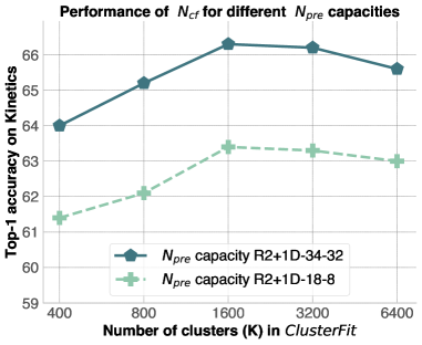
Figure 5: Relative Model Capacity of ${\color[rgb]{0.5,0.0,0.5}\mathrm{N_{pre}}}$ and ${\color[rgb]{0.0,0.5,0.0}\mathrm{N_{cf}}}$ (section 5.1): We fix ${\color[rgb]{0.0,0.5,0.0}\mathrm{N_{cf}}}$ $=$ R(2+1)D-18. We vary (a) ${\color[rgb]{0.5,0.0,0.5}\mathrm{N_{pre}}}$ $=$ ${\color[rgb]{0.0,0.5,0.0}\mathrm{N_{cf}}}$ $=$ R(2+1)D-18 (light green) and (b) ${\color[rgb]{0.5,0.0,0.5}\mathrm{N_{pre}}}$ $>$ ${\color[rgb]{0.0,0.5,0.0}\mathrm{N_{cf}}}$, where ${\color[rgb]{0.5,0.0,0.5}\mathrm{N_{pre}}}$ $=$ R(2+1)D-34 (dark green). We report the transfer performance of the ${\color[rgb]{0.0,0.5,0.0}\mathrm{N_{cf}}}$ model for cases (a) and (b) on Kinetics. A higher capacity ${\color[rgb]{0.5,0.0,0.5}\mathrm{N_{pre}}}$ results in better transfer performance.

5.1 Relative model capacity of ${\color[rgb]{0.5,0.0,0.5}\mathrm{N_{pre}}}$ and ${\color[rgb]{0.0,0.5,0.0}\mathrm{N_{cf}}}$

The relative model capacities of ${\color[rgb]{0.5,0.0,0.5}\mathrm{N_{pre}}}$ and ${\color[rgb]{0.0,0.5,0.0}\mathrm{N_{cf}}}$ can impact the final transfer performance of ${\color[rgb]{0.0,0.5,0.0}\mathrm{N_{cf}}}$. To study this behavior, we fix ${\color[rgb]{0.5,0.0,0.5}\mathrm{D_{pre}}}$ $=$ IG-Verb-19M and ${\color[rgb]{0.0,0.5,0.0}\mathrm{D_{cf}}}$ $=$ IG-Verb-62M, and ${\color[rgb]{0.0,0.5,0.0}\mathrm{N_{cf}}}$ $=$ R(2+1)D-18. We vary the architecture of ${\color[rgb]{0.5,0.0,0.5}\mathrm{N_{pre}}}$ as follows: (a) ${\color[rgb]{0.5,0.0,0.5}\mathrm{N_{pre}}}$ $=$ ${\color[rgb]{0.0,0.5,0.0}\mathrm{N_{cf}}}$ $=$ R(2+1)D-18; (b) ${\color[rgb]{0.5,0.0,0.5}\mathrm{N_{pre}}}$ $>$ ${\color[rgb]{0.0,0.5,0.0}\mathrm{N_{cf}}}$, where ${\color[rgb]{0.5,0.0,0.5}\mathrm{N_{pre}}}$ $=$ R(2+1)D-34 model ($64M$ parameters) and thus higher capacity than ${\color[rgb]{0.0,0.5,0.0}\mathrm{N_{cf}}}$ ($33M$ parameters).

From fig. 5, we observe a consistent improvement of $2\%-3\%$ across different values of $K$ when a higher capacity model was used as ${\color[rgb]{0.5,0.0,0.5}\mathrm{N_{pre}}}$. This result is intuitive and indicates that a higher capacity ${\color[rgb]{0.5,0.0,0.5}\mathrm{N_{pre}}}$ yields richer visual features for clustering and thus improves the transfer learning performance. We note that in the aforementioned case (b), our framework can be viewed to be distilling knowledge from a higher capacity teacher model (${\color[rgb]{0.5,0.0,0.5}\mathrm{N_{pre}}}$) to a lower-capacity student model (${\color[rgb]{0.0,0.5,0.0}\mathrm{N_{cf}}}$).

5.2 Unsupervised vs. Per-Label Clustering

Figure 6: Unsupervised vs. Per-Label Clustering (section 5.2): In per-label clustering, we retain the semantic information of the class labels and cluster videos belonging to each label. We note that for all values of $K$, unsupervised clustering used in ClusterFit yields better transfer learning performance on Kinetics and Sports1M.

As noted before, the clustering step in ClusterFit is ‘unsupervised’ because it discards the labels associated with ${\color[rgb]{0.0,0.5,0.0}\mathrm{D_{cf}}}$ and operates purely on the feature representations. But is there any advantage of using the semantic information of labels in ${\color[rgb]{0.0,0.5,0.0}\mathrm{D_{cf}}}$ for clustering? To address this question, we formulate a per-label clustering setup. Specifically, given each label $l$, we cluster videos belonging to it into $k_{l}$ clusters. We treat $K=\{k_{l}:\forall l\}$ as pseudo-labels to train ${\color[rgb]{0.0,0.5,0.0}\mathrm{N_{cf}}}$. Each $k_{l}$ is defined to be proportional to $\sqrt{n_{l}}$ where $n_{l}$ denotes the number of videos associated with the label $l$.

Figure 6 compares the two clustering approaches on Kinetics and Sports1M. We observe that on both datasets, unsupervised clustering consistently outperforms per-label clustering across all values of $K$. We believe that by operating purely on video features, the unsupervised approach effectively captures the visual coherence in ${\color[rgb]{0.0,0.5,0.0}\mathrm{D_{cf}}}$. Consequently, factors around label noise such as wrong / missing labels and lexical ambiguity are being automatically addressed in the unsupervised framework, leading to superior performance over per-label clustering.

5.3 Properties of ${\color[rgb]{0.5,0.0,0.5}\mathrm{D_{pre}}}$

In this section, we address the following question: what constitutes a valuable pre-training label space (${\color[rgb]{0.5,0.0,0.5}\mathrm{D_{pre}}}$) and how to construct one? Towards this end, we study two properties of ${\color[rgb]{0.5,0.0,0.5}\mathrm{D_{pre}}}$: the nature of it’s labels and their cardinality. We refer the readers to the supplementary material for discussion on the nature of labels.

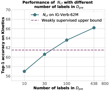
Figure 7: Effect of number of labels in ${\color[rgb]{0.5,0.0,0.5}\mathrm{N_{pre}}}$ ( section 5.3). We design $4$ different ${\color[rgb]{0.5,0.0,0.5}\mathrm{D_{pre}}}$, each with $19M$ videos but #labels $=\{10,30,100,438\}$, $K=3200$ and ${\color[rgb]{0.0,0.5,0.0}\mathrm{D_{cf}}}$ $=$ IG-Verb-62M. X-axis is in log-linear scale.

Number of labels in ${\color[rgb]{0.5,0.0,0.5}\mathrm{D_{pre}}}$: We now study how varying the number of labels in ${\color[rgb]{0.5,0.0,0.5}\mathrm{D_{pre}}}$ effects ClusterFit. To study this, we fix the total number of unique videos in ${\color[rgb]{0.5,0.0,0.5}\mathrm{D_{pre}}}$ to $19M$ and vary the number of pre-training labels. First, we consider IG-Verb-62M and rank it’s $438$ weak verb labels by their frequency of occurrence. Next, we construct $4$ different ${\color[rgb]{0.5,0.0,0.5}\mathrm{D_{pre}}}$ datasets by considering unique $19M$ videos tagged with top-m verbs, where $m=\{10,30,100,438\}$. Note that for a fixed number of videos in ${\color[rgb]{0.5,0.0,0.5}\mathrm{D_{pre}}}$, reducing the number of labels implies reduced content diversity.

From Figure 7, we observe that the transfer learning performance increases log-linearly with the number of pre-training labels in ${\color[rgb]{0.5,0.0,0.5}\mathrm{D_{pre}}}$. When we use just the top-10 verbs ($m=10$), accuracy drops by around $9\%$ compared to $m=438$. This indicates that label space diversity is essential to generate good quality clusters. However, when $m=100$, ${\color[rgb]{0.0,0.5,0.0}\mathrm{N_{cf}}}$ is within $2\%$ of the accuracy obtained when using all $438$ verbs, and it outperform its weakly supervised pre-trained counterpart which uses 62M videos and all 438 verbs. This experiment clearly demonstrates the utility of our approach in designing a generic pre-training label space with minimal effort. Contrary to [38, 20] which propose careful, manual label engineering, ClusterFit offers an easy way to construct a powerful, generalizable pre-training label space. Increasing the label space granularity is as simple as increasing the number of clusters in ClusterFit and requires no additional manual effort.

6 Discussion

In this work, we presented ClusterFit, a simple approach to significantly improve the generalizability of features learnt in weakly-supervised and self-supervised frameworks for images and videos. While models trained in these frameworks are prone to overfit to the pre-training objective, ClusterFit combats this issue by first clustering the original feature space and re-learning a new model on cluster assignments. Clustering in CF may be viewed as a lossy compression scheme that effectively captures the essential visual invariances in the feature space. Thus, predicting the cluster labels gives the ‘re-learned’ network an opportunity to learn features that are less sensitive to the original pre-training objective, making them more transferable.

While the clustering step in ClusterFit is unsupervised, in practice, domain knowledge from downstream target tasks can be used to guide clustering and possibly improve the transfer learning performance. Additionally, we found that in its current unsupervised form, iterative application of CF provides little improvements; incorporating domain knowledge could be a potential solution.

ClusterFit is a universal framework - it is scalable and imposes no restrictions on model architectures, modalities of data, and forms of supervision. Future research should take advantage of its flexibility and combine different types of pre-trained models for learning cluster assignments in a multi-task manner. Using evidence accumulation methods [50, 41, 17] for clustering is another worthwhile direction to explore.

Acknowledgments:

We would like to thank Rob Fergus, and Zhenheng Yang for feedback on the manuscript; Filip Radenovic, and Vignesh Ramanathan for feedback on the experimental setup; Laurens van der Maaten, Larry Zitnick, Armand Joulin, and Xinlei Chen for helpful discussions.

Supplemental Material

Appendix A Details on baseline methods

Details on distillation

The distillation loss function is a convex combination of two individual losses - (1) a loss that tries to match the ‘soft’ target outputs by a teacher model, i.e., a probability distribution computed by applying a softmax function on the logits of a teacher model using a temperature $T$; (2) a cross-entropy loss that tries to match the predictions with the ground truth labels for each datapoint. The two losses are combined with a convex combination ($\alpha$ used for the first loss and $1-\alpha$ used for the second loss). We performed a grid search to find the optimal values for temperature $T$ and weight $\alpha$. We set these values as $T=20$ and $\alpha=0.75$.

Details on prototype baseline

Prototype method is a simplified version of k-means with only one iteration and controlled initialization. Similar to k-means, it consists of two steps: (1) cluster center initialization and (2) cluster label reassignment. In step 1, we compute an average of the visual features of all datapoints (videos or images) belonging to each label. These visual embeddings per label are chosen as cluster centers. Then, in step 2, data points are re-assigned to their nearest cluster centers (computed from step 1). Finally, the newly assigned cluster id is used as the label in training ${\color[rgb]{0.0,0.5,0.0}\mathrm{N_{cf}}}$. Prototype method is limited to (weakly) supervised setting as it requires label information in step 1. Also, it yields the same number of clusters as the cardinality of the input label space.

Appendix B Weakly supervised Images

We provide details for Section 4.1.1 of the main paper.

Details on the IG-ImageNet dataset

We get $1500(>1000)$ total hashtags because multiple hashtags may map to the same ImageNet synset.

Details on pre-training

We follow the implementation from [38]. All models are trained using Synchronized stochastic gradient descent (SGD) on $128$ GPUs across $16$ machines. Each GPU processes $32$ images at a time. All the pre-training runs process $2B$ images in total. An initial learning rate of $1.6$ is used and decreased by a factor of $2$ at $13$ equally spaced steps.

Details on ClusterFit

k-means: Since number of images are very large, we randomly sub-sample $200M$ images and perform $30$ iterations of k-means clustering on them. We use the cluster centers obtained in this step, and then perform $5$ more iterations of k-means with all the 1B images.

Transfer Learning Hyperparameters

We closely follow transfer learning settings in [38] and apply parameter sweep on learning rate for different target datasets.

Appendix C Weakly supervised Videos

We provide details for Section 4.1.2 of the main paper.

Details on the IG-Verb dataset

We strictly follow [20] to construct large-scale weakly supervised video datasets. We borrow label space from public datasets and crawl videos that contain matching hashtags from a social website. Given the great amount of noise in web data, labels with at least 50 matching videos are finally retained. IG-Verb-62M dataset consists of 438 verbs, a union of Kinetics and VerbNet [57] verbs, and 62M videos with at least one matching hashtag. If multiple hashtags are attached to one video, one hashtag/verb is randomly picked as label. We also follow the tail-preserving strategy in [20] to construct IG-verb-19M, which is a subset of IG-Verb-62M.

Details on the IG-Kinetics and IG-Noun dataset

Following the same rules as above, we construct IG-Kinetics-19M comprising $359$ labels from Kinetics label space, and IG-Noun-19M comprising $1438$ labels from ImageNet synsets. These two datasets are used later in studying the effect of nature of labels in ${\color[rgb]{0.5,0.0,0.5}\mathrm{D_{pre}}}$.

Details on pre-training

Training for both ${\color[rgb]{0.5,0.0,0.5}\mathrm{N_{pre}}}$ and ${\color[rgb]{0.0,0.5,0.0}\mathrm{N_{cf}}}$ follow the same setting. $128$ GPUs across $16$ machines are used. Each GPU processes $6$ videos at a time and batch normalization [30] is applied to all convolutional layers on each GPU. All the pre-training experiments process $490M$ videos in total across all epochs. We closely follow the training hyper-parameters mentioned in [20].

Transfer Learning Hyperparameters

We closely follow transfer learning settings in [20] and apply parameter sweep on learning rate for different target datasets.

Appendix D Self-supervised Images

We provide details for Section 4.2 of the main paper.

Self-supervised Pre-training (${\color[rgb]{0.5,0.0,0.5}\mathrm{N_{pre}}}$)

The Jigsaw and RotNet model pre-training is based on the code release from [22, 33, 21]. We use a standard ResNet-50 model for both methods. We use a batchsize of $32$ per GPU, a total of 8 GPUs and optimize these models using mini-batch SGD for a total of $105$ epochs with an initial learning rate of $0.1$, decayed by a factor of $10$ after every $30$ epochs.

Details on Jigsaw ${\color[rgb]{0.5,0.0,0.5}\mathrm{N_{pre}}}$

We follow [22, 42] to construct the ‘jigsaw puzzles’ from the images. We first resize the image (maintaining aspect ratio) to make its shortest side $255$, and then extract a random square crop of $255\times 255$ from it. This crop is divided into a $3\times 3$ grid and a random crop of $64\times 64$ is extracted from each of the 9 grids to get 9 patches. The patches are input individually to the network to obtain their features, and are concatenated in a random order. Finally, the concatenated features are input to a classification layer which predicts the ‘class index’ of the random permutation used to concatenate the features. We use $2000$ permutations as used in [22].

Details on RotNet ${\color[rgb]{0.5,0.0,0.5}\mathrm{N_{pre}}}$

We follow [21, 33] and apply a random rotation from $\{0^{\circ},90^{\circ},180^{\circ},270^{\circ}\}$ to the input image. The network is trained (4-way classification) to predict the index of the rotation applied to the input.

Details on ClusterFit

We extract features (res5 after average pooling, 2048 dimensional vector) from each of the self-supervised ${\color[rgb]{0.5,0.0,0.5}\mathrm{N_{pre}}}$ networks on the ImageNet-1K dataset (train split of 1.28M images). We then $l_{2}$ normalize the features and use k-means to cluster these images and obtain pseudo-labels as the cluster assignments for each point.

We also trained a version of ${\color[rgb]{0.0,0.5,0.0}\mathrm{N_{cf}}}$ by clustering the res4 features from ${\color[rgb]{0.5,0.0,0.5}\mathrm{N_{pre}}}$. We found that this version gave similar performance to the ${\color[rgb]{0.0,0.5,0.0}\mathrm{N_{cf}}}$ trained on cluster assignments from the res5 layer of ${\color[rgb]{0.5,0.0,0.5}\mathrm{N_{pre}}}$.

Transfer Learning Hyperparameters

We train linear classifiers on fixed features. Following [22] we use mini-batch SGD with a batchsize of $256$, learning rate of $0.01$ dropped by a factor of 10 after two equally spaced intervals, momentum of $0.9$, and weight decay of $5\times 10^{-4}$. The features from each layer (conv1, res4, res5 etc.) are average pooled to get a feature of about $9000$ dimensions each. We try to keep the number of parameter updates for training the linear models are roughly constant across all the transfer datasets. Thus, the models are trained for $28$ epochs on ImageNet-1K (1.28M training images), $14$ epochs on Places205 (2.4M training images) and for $84$ epochs on iNaturalist-2018 (437K training images). We follow [22] and train linear SVMs for the VOC07 transfer task.

Transfer Learning Results

In Section 4.2 of the main paper, we showed transfer learning results when ${\color[rgb]{0.5,0.0,0.5}\mathrm{D_{pre}}}={\color[rgb]{0.0,0.5,0.0}\mathrm{D_{cf}}}=$ ImageNet-1K and the architecture of ${\color[rgb]{0.5,0.0,0.5}\mathrm{N_{pre}}}$ and ${\color[rgb]{0.0,0.5,0.0}\mathrm{N_{cf}}}$ was ResNet-50. In Table 7 we show results for different values of the number of cluster, $K$, used to generate the pseudo-labels. Although the performance of ${\color[rgb]{0.0,0.5,0.0}\mathrm{N_{cf}}}$ increases as the number of clusters $K$ increases, we observe that ClusterFit provides significant improvements over the pre-trained ${\color[rgb]{0.5,0.0,0.5}\mathrm{N_{pre}}}$ at smaller values ($K=1000$).

Method	${\color[rgb]{0.0,0.3,0.8}\mathrm{T_{tar}}}$
	ImageNet-1K	VOC07	Places205	iNaturalist
Jigsaw ${\color[rgb]{0.5,0.0,0.5}\mathrm{N_{pre}}}$	46.0	66.1	39.9	22.1
Jigsaw ${\color[rgb]{0.0,0.5,0.0}\mathrm{N_{cf}}}$ ($K=1000$)	50.2	66.2	42.5	24.5
Jigsaw ${\color[rgb]{0.0,0.5,0.0}\mathrm{N_{cf}}}$ ($K=4000$)	51.6	67.8	42.4	27.2
Jigsaw ${\color[rgb]{0.0,0.5,0.0}\mathrm{N_{cf}}}$ ($K=16000$)	55.2	69.5	45.0	29.8
RotNet ${\color[rgb]{0.5,0.0,0.5}\mathrm{N_{pre}}}$	48.9	63.9	41.4	23.0
RotNet ${\color[rgb]{0.0,0.5,0.0}\mathrm{N_{cf}}}$ ($K=1000$)	51.8	67.2	42.6	25.2
RotNet ${\color[rgb]{0.0,0.5,0.0}\mathrm{N_{cf}}}$ ($K=4000$)	52.3	67.4	43.4	26.8
RotNet ${\color[rgb]{0.0,0.5,0.0}\mathrm{N_{cf}}}$ ($K=16000$)	56.1	70.9	44.8	28.4

Table 7: Self-supervised methods: We apply ClusterFit to self-supervised methods and evaluate them following the setup in [22] on four datasets by training a linear classifier on fixed features. All methods use the ResNet-50 architecture for ${\color[rgb]{0.5,0.0,0.5}\mathrm{N_{pre}}}$ and ${\color[rgb]{0.0,0.5,0.0}\mathrm{N_{cf}}}$. We report the performance of the best performing layer for each method and use the mean Average Precision (mAP) metric for the VOC07 dataset and top-1 accuracy for all other datasets. We show results for different values of $K$ used to generate the pseudo-labels.

Distillation is not a valid baseline

In self-supervised methods like Jigsaw and RotNet, the predictions depend upon the image transformation (permutation of patches for Jigsaw or the rotations for RotNet) applied to the input. Thus, given an untransformed input image, the self-supervised methods do not produce a ‘distribution’ over the possible set of output values. For example, in RotNet, if we only pass an untransformed image, the network predicts (with high confidence) that the image is rotated by $0^{\circ}$, and thus the ‘distribution’ over the possible rotation values of the input is not very meaningful to use in a distillation method. For Jigsaw, since the output is the index of the permutation applied to the input patches, the distribution produced for a ‘regular’ input is not meaningful.

Appendix E Bonus: Multi-task Self-supervised Learning

We study the generalization of ClusterFit by using it for self-supervised multi-task learning. We take a pre-trained network ${\color[rgb]{0.5,0.0,0.5}\mathrm{N_{pre}}}$ on Jigsaw and use it to compute the pseudo-labels (via clustering) on ${\color[rgb]{0.0,0.5,0.0}\mathrm{D_{cf}}}$. We repeat the process for another ${\color[rgb]{0.5,0.0,0.5}\mathrm{N_{pre}}}$ trained on RotNet to get a different set of pseudo-labels on ${\color[rgb]{0.0,0.5,0.0}\mathrm{D_{cf}}}$. We treat these two sets of pseudo-labels as two different multi-class classification problems and train a new ${\color[rgb]{0.0,0.5,0.0}\mathrm{N_{cf}}}$ from scratch using these labels. Thus, ${\color[rgb]{0.0,0.5,0.0}\mathrm{N_{cf}}}$ is trained with two different fully-connected layers, each of which predicts the pseudo-labels from a different ${\color[rgb]{0.5,0.0,0.5}\mathrm{N_{pre}}}$. We sum the losses from these two layers and optimize the network.

We follow the setup from section 4.2, and use the ResNet-50 architecture for both ${\color[rgb]{0.5,0.0,0.5}\mathrm{N_{pre}}}$ and ${\color[rgb]{0.0,0.5,0.0}\mathrm{N_{cf}}}$, and set ${\color[rgb]{0.5,0.0,0.5}\mathrm{D_{pre}}}\!=\!{\color[rgb]{0.0,0.5,0.0}\mathrm{D_{cf}}}\!=\!$ImageNet-1K. The linear evaluation results are presented in Table 8. This näive way of multi-task learning using ClusterFit still improves the performance and provides gains of 8 points on ImageNet-1K, iNaturalist in top-1 accuracy and VOC07 mAP compared to the ${\color[rgb]{0.5,0.0,0.5}\mathrm{N_{pre}}}$ models. The multi-task models also improve over the single task ${\color[rgb]{0.0,0.5,0.0}\mathrm{N_{cf}}}$ models.

Method	${\color[rgb]{0.0,0.3,0.8}\mathrm{T_{tar}}}$
	ImageNet-1K	VOC07	Places205	iNaturalist
Jigsaw ${\color[rgb]{0.5,0.0,0.5}\mathrm{N_{pre}}}$	46.0	66.1	39.9	22.1
Jigsaw ${\color[rgb]{0.5,0.0,0.5}\mathrm{N_{pre}}}2\times$	45.1	65.4	38.7	21.8
Jigsaw ${\color[rgb]{0.0,0.5,0.0}\mathrm{N_{cf}}}$ (Ours)	55.2	69.5	45.0	29.8
RotNet ${\color[rgb]{0.5,0.0,0.5}\mathrm{N_{pre}}}$	48.9	63.9	41.4	23.0
RotNet ${\color[rgb]{0.5,0.0,0.5}\mathrm{N_{pre}}}2\times$	50.0	64.9	42.9	25.3
RotNet ${\color[rgb]{0.0,0.5,0.0}\mathrm{N_{cf}}}$ (Ours)	56.1	70.9	44.8	28.4
Jigsaw + RotNet ${\color[rgb]{0.0,0.5,0.0}\mathrm{N_{cf}}}$	57.0	72.8	46.2	31.6
(Ours, Multi-task)

Table 8: Multi-task Self-supervised: We show that ClusterFit can be used for easy multi-task learning. We apply ClusterFit to self-supervised methods and evaluate them following the setup in [22] on four datasets by training a linear classifier on fixed features. All methods use the ResNet-50 architecture for ${\color[rgb]{0.5,0.0,0.5}\mathrm{N_{pre}}}$ and ${\color[rgb]{0.0,0.5,0.0}\mathrm{N_{cf}}}$. We report the performance of the best performing layer for each method and use the mean Average Precision (mAP) metric for the VOC07 dataset and top-1 accuracy for all other datasets.

Appendix F Analysis of ClusterFit

We provide details for Section 5 of the main paper.

Details on ${\color[rgb]{0.0,0.5,0.0}\mathrm{N_{cf}}}$ training:

In Section 5, we use R(2+1)D-18 as ${\color[rgb]{0.0,0.5,0.0}\mathrm{N_{cf}}}$ and IG-Verb-62M as ${\color[rgb]{0.0,0.5,0.0}\mathrm{D_{cf}}}$. Training is done with $64$ GPUs across $8$ machines. Each GPU processes $16$ videos at a time and batch normalization[30] is applied to all convolutional layers on each GPU. The training processes 250M video in total. An initial learning rate of 0.005 per GPU is applied and decreased by a factor of 2 at 13 equally spaced steps.

Effect of nature of labels in ${\color[rgb]{0.5,0.0,0.5}\mathrm{D_{pre}}}$:

In the main paper, we have shown results where ${\color[rgb]{0.5,0.0,0.5}\mathrm{N_{pre}}}$ is pre-trained on labels that are verbs (i.e., on IG-Verb-19M dataset). It is natural to question: how does the choice of ${\color[rgb]{0.5,0.0,0.5}\mathrm{D_{pre}}}$’s label space effect ClusterFit? To study this, we vary ${\color[rgb]{0.5,0.0,0.5}\mathrm{D_{pre}}}$ by changing the properties of their labels, but keeping the volume of the data fixed. All other settings, including ${\color[rgb]{0.0,0.5,0.0}\mathrm{D_{cf}}}$, ${\color[rgb]{0.5,0.0,0.5}\mathrm{N_{pre}}}$ and ${\color[rgb]{0.0,0.5,0.0}\mathrm{N_{cf}}}$, are fixed. Specifically, we consider three ${\color[rgb]{0.0,0.5,0.0}\mathrm{D_{cf}}}$ datasets with $19M$ videos each: (a) IG-Verb-19M, (b) IG-Noun-19M and (c) IG-Kinetics-19M. Next, we pre-trained three separate ${\color[rgb]{0.5,0.0,0.5}\mathrm{N_{pre}}}$ on these datasets. Then, we use ${\color[rgb]{0.0,0.5,0.0}\mathrm{D_{cf}}}$ = IG-Verb-62M to apply ClusterFit on each of them, and get three ${\color[rgb]{0.0,0.5,0.0}\mathrm{N_{cf}}}$. Finally, transfer learning is done on three ${\color[rgb]{0.0,0.5,0.0}\mathrm{N_{cf}}}$.

Figure 8: Nature of pre-training labels  (appendix F):

Figure 8 shows the transfer learning performance on Kinetics and Sports1M, where ${\color[rgb]{0.0,0.5,0.0}\mathrm{D_{cf}}}$ is fixed to IG-Verb-62M. For a fair comparison, we report the performance when ${\color[rgb]{0.5,0.0,0.5}\mathrm{N_{pre}}}$ is pre-trained on IG-Verb-62M, without applying ClusterFit (dotted magenta line). We make the following observations: first, all three ${\color[rgb]{0.5,0.0,0.5}\mathrm{D_{pre}}}$ datasets show significant improvements over the weakly-supervised upper bound upon applying ClusterFit, further reaffirming its generalizability. Second, ${\color[rgb]{0.5,0.0,0.5}\mathrm{D_{pre}}}$ $=$ IG-Kinetics-19M yields a slightly higher performance on Kinetics, which indicates that prior domain knowledge of the downstream target task can help design ${\color[rgb]{0.5,0.0,0.5}\mathrm{D_{pre}}}$ for maximum benefit (as observed in [38, 20]).

References

- [1] Rohan Anil, Gabriel Pereyra, Alexandre Passos, Robert Ormandi, George E Dahl, and Geoffrey E Hinton. Large scale distributed neural network training through online distillation. arXiv preprint arXiv:1804.03235, 2018.
- [2] Relja Arandjelovic and Andrew Zisserman. Look, listen and learn. In ICCV, 2017.
- [3] Relja Arandjelovic and Andrew Zisserman. Objects that sound. In ECCV, 2018.
- [4] Jimmy Ba and Rich Caruana. Do deep nets really need to be deep? In Advances in neural information processing systems, pages 2654–2662, 2014.
- [5] Piotr Bojanowski and Armand Joulin. Unsupervised learning by predicting noise. In ICML, 2017.
- [6] Mathilde Caron, Piotr Bojanowski, Armand Joulin, and Matthijs Douze. Deep clustering for unsupervised learning of visual features. In ECCV, 2018.
- [7] Mathilde Caron, Piotr Bojanowski, Julien Mairal, and Armand Joulin. Unsupervised pre-training of image features on non-curated data. In ICCV, 2019.
- [8] D. Tran, H. Wang, L. Torresani, J. Ray, Y. LeCun, and M. Paluri. A closer look at spatiotemporal convolutions for action recognition. CVPR, 2018.
- [9] Virginia R de Sa. Learning classification with unlabeled data. In NIPS, 1994.
- [10] Jia Deng, Wei Dong, Richard Socher, Li-Jia Li, Kai Li, and Li Fei-Fei. Imagenet: A large-scale hierarchical image database. 2009.
- [11] E. Denton, J. Weston, M. Paluri, L. Bourdev, and R. Fergus. User conditional hashtag prediction for images. In Proc. KDD, pages 1731–1740, 2015.
- [12] Aditya Deshpande, Jason Rock, and David Forsyth. Learning large-scale automatic image colorization. In ICCV, 2015.
- [13] Carl Doersch, Abhinav Gupta, and Alexei A Efros. Unsupervised visual representation learning by context prediction. In ICCV, pages 1422–1430, 2015.
- [14] Alexey Dosovitskiy, Philipp Fischer, Jost Tobias Springenberg, Martin Riedmiller, and Thomas Brox. Discriminative unsupervised feature learning with exemplar convolutional neural networks. TPAMI, 38(9):1734–1747, 2016.
- [15] M. Everingham, S. M. A. Eslami, L. Van Gool, C. K. I. Williams, J. Winn, and A. Zisserman. The pascal visual object classes challenge: A retrospective. International Journal of Computer Vision, 111(1):98–136, Jan. 2015.
- [16] Basura Fernando, Hakan Bilen, Efstratios Gavves, and Stephen Gould. Self-supervised video representation learning with odd-one-out networks. In CVPR, 2017.
- [17] Ana LN Fred and Anil K Jain. Data clustering using evidence accumulation. In Object recognition supported by user interaction for service robots, volume 4, pages 276–280. IEEE, 2002.
- [18] Tommaso Furlanello, Zachary C Lipton, Michael Tschannen, Laurent Itti, and Anima Anandkumar. Born again neural networks. arXiv preprint arXiv:1805.04770, 2018.
- [19] Ruohan Gao, Rogerio Feris, and Kristen Grauman. Learning to separate object sounds by watching unlabeled video. In ECCV, 2018.
- [20] Deepti Ghadiyaram, Matt Feiszli, Du Tran, Xueting Yan, Heng Wang, and Dhruv Mahajan. Large-scale weakly-supervised pre-training for video action recognition. arXiv preprint arXiv:1905.00561, 2019.
- [21] Spyros Gidaris, Praveer Singh, and Nikos Komodakis. Unsupervised representation learning by predicting image rotations. arXiv preprint arXiv:1803.07728, 2018.
- [22] Priya Goyal, Dhruv Mahajan, Abhinav Gupta, and Ishan Misra. Scaling and benchmarking self-supervised visual representation learning. arXiv preprint arXiv:1905.01235, 2019.
- [23] Raghav Goyal, Samira Ebrahimi Kahou, Vincent Michalski, Joanna Materzynska, Susanne Westphal, Heuna Kim, Valentin Haenel, Ingo Fruend, Peter Yianilos, Moritz Mueller-Freitag, et al. The “something something” video database for learning and evaluating visual common sense. In ICCV, 2017.
- [24] Sam Gross, Marc’Aurelio Ranzato, and Arthur Szlam. Hard mixtures of experts for large scale weakly supervised vision. In CVPR, 2017.
- [25] Raia Hadsell, Sumit Chopra, and Yann LeCun. Dimensionality reduction by learning an invariant mapping. In CVPR, 2006.
- [26] James Hays and Alexei A Efros. Im2gps: estimating geographic information from a single image. In 2008 ieee conference on computer vision and pattern recognition, pages 1–8. IEEE, 2008.
- [27] Kaiming He, Xiangyu Zhang, Shaoqing Ren, and Jian Sun. Deep residual learning for image recognition. In CVPR, 2016.
- [28] Geoffrey Hinton, Oriol Vinyals, and Jeff Dean. Distilling the knowledge in a neural network. arXiv preprint arXiv:1503.02531, 2015.
- [29] R Devon Hjelm, Alex Fedorov, Samuel Lavoie-Marchildon, Karan Grewal, Phil Bachman, Adam Trischler, and Yoshua Bengio. Learning deep representations by mutual information estimation and maximization. arXiv preprint arXiv:1808.06670, 2018.
- [30] Sergey Ioffe and Christian Szegedy. Batch normalization: Accelerating deep network training by reducing internal covariate shift. arXiv preprint arXiv:1502.03167, 2015.
- [31] Armand Joulin, Laurens van der Maaten, Allan Jabri, and Nicolas Vasilache. Learning visual features from large weakly supervised data. In ECCV, 2016.
- [32] Andrej Karpathy, George Toderici, Sanketh Shetty, Thomas Leung, Rahul Sukthankar, and Li Fei-Fei. Large-scale video classification with convolutional neural networks. In Proceedings of the IEEE conference on Computer Vision and Pattern Recognition, pages 1725–1732, 2014.
- [33] Alexander Kolesnikov, Xiaohua Zhai, and Lucas Beyer. Revisiting self-supervised visual representation learning. arXiv preprint arXiv:1901.09005, 2019.
- [34] Gustav Larsson, Michael Maire, and Gregory Shakhnarovich. Learning representations for automatic colorization. In ECCV, 2016.
- [35] Gustav Larsson, Michael Maire, and Gregory Shakhnarovich. Colorization as a proxy task for visual understanding. In CVPR, 2017.
- [36] A. Li, A. Jabri, A. Joulin, and L.J.P. van der Maaten. Learning visual n-grams from web data. In Proc. ICCV, 2017.
- [37] Pauline Luc, Natalia Neverova, Camille Couprie, Jakob Verbeek, and Yann LeCun. Predicting deeper into the future of semantic segmentation. In ICCV, 2017.
- [38] Dhruv Mahajan, Ross Girshick, Vignesh Ramanathan, Kaiming He, Manohar Paluri, Yixuan Li, Ashwin Bharambe, and Laurens van der Maaten. Exploring the limits of weakly supervised pretraining. In ECCV, 2018.
- [39] Ishan Misra, C Lawrence Zitnick, and Martial Hebert. Shuffle and learn: unsupervised learning using temporal order verification. In ECCV, 2016.
- [40] Hossein Mobahi, Ronan Collobert, and Jason Weston. Deep learning from temporal coherence in video. In ICML, 2009.
- [41] Nam Nguyen and Rich Caruana. Consensus clusterings. In Seventh IEEE International Conference on Data Mining (ICDM 2007), pages 607–612. IEEE, 2007.
- [42] Mehdi Noroozi and Paolo Favaro. Unsupervised learning of visual representations by solving jigsaw puzzles. In ECCV, 2016.
- [43] Mehdi Noroozi, Hamed Pirsiavash, and Paolo Favaro. Representation learning by learning to count. In ICCV, 2017.
- [44] Mehdi Noroozi, Ananth Vinjimoor, Paolo Favaro, and Hamed Pirsiavash. Boosting self-supervised learning via knowledge transfer. In CVPR, 2018.
- [45] Aaron van den Oord, Yazhe Li, and Oriol Vinyals. Representation learning with contrastive predictive coding. arXiv preprint arXiv:1807.03748, 2018.
- [46] Andrew Owens, Jiajun Wu, Josh H McDermott, William T Freeman, and Antonio Torralba. Ambient sound provides supervision for visual learning. In ECCV, 2016.
- [47] Olga Russakovsky, Jia Deng, Hao Su, Jonathan Krause, Sanjeev Satheesh, Sean Ma, Zhiheng Huang, Andrej Karpathy, Aditya Khosla, Michael Bernstein, Alexander C. Berg, and Li Fei-Fei. ImageNet Large Scale Visual Recognition Challenge. IJCV, 115, 2015.
- [48] F. Schroff, D. Kalenichenko, and J. Philbin. Facenet: A unified embedding for face recognition and clustering. In CVPR, 2015.
- [49] Jake Snell, Kevin Swersky, and Richard Zemel. Prototypical networks for few-shot learning. In Advances in Neural Information Processing Systems, pages 4077–4087, 2017.
- [50] Alexander Strehl and Joydeep Ghosh. Cluster ensembles—a knowledge reuse framework for combining multiple partitions. Journal of machine learning research, 3(Dec):583–617, 2002.
- [51] Chen Sun, Abhinav Shrivastava, Saurabh Singh, and Abhinav Gupta. Revisiting unreasonable effectiveness of data in deep learning era. In ICCV, 2017.
- [52] Y. Taigman, M. Yang, M.A. Ranzato, and L. Wolf. Web-scale training for face identification. In CVPR, 2015.
- [53] Bart Thomee, David A Shamma, Gerald Friedland, Benjamin Elizalde, Karl Ni, Douglas Poland, Damian Borth, and Li-Jia Li. Yfcc100m: The new data in multimedia research. Communications of the ACM, 59(2):64–73, 2016.
- [54] Naftali Tishby and Noga Zaslavsky. Deep learning and the information bottleneck principle. In 2015 IEEE Information Theory Workshop (ITW), pages 1–5. IEEE, 2015.
- [55] Grant Van Horn, Oisin Mac Aodha, Yang Song, Yin Cui, Chen Sun, Alex Shepard, Hartwig Adam, Pietro Perona, and Serge Belongie. The inaturalist species classification and detection dataset. In CVPR, pages 8769–8778, 2018.
- [56] A. Veit, M. Nickel, S. Belongie, and L.J.P. van der Maaten. Separating self-expression and visual content in hashtag supervision. In arXiv 1711.09825, 2017.
- [57] VerbNet. VerbNet : A Computational Lexical Resource for Verbs. [Online] Available https://verbs.colorado.edu/verbnet/.
- [58] Nam Vo, Nathan Jacobs, and James Hays. Revisiting im2gps in the deep learning era. In Proceedings of the IEEE International Conference on Computer Vision, pages 2621–2630, 2017.
- [59] W. Kay, J. Carreira, K. Simonyan, B. Zhang, C. Hillier, S. Vijayanarasimhan, F. Viola, T. Green, T. Back, P. Natsev, M. Suleyman, and A. Zisserman. The kinetics human action video dataset. arXiv:1705.06950, 2017.
- [60] Zhirong Wu, Yuanjun Xiong, Stella X Yu, and Dahua Lin. Unsupervised feature learning via non-parametric instance discrimination. In CVPR, 2018.
- [61] Junyuan Xie, Ross Girshick, and Ali Farhadi. Unsupervised deep embedding for clustering analysis. In ICML, pages 478–487, 2016.
- [62] I. Zeki Yalniz, Hervé Jégou, Kan Chen, Manohar Paluri, and Dhruv Mahajan. Billion-scale semi-supervised learning for image classification. CoRR, abs/1905.00546, 2019.
- [63] Richard Zhang, Phillip Isola, and Alexei A Efros. Colorful image colorization. In ECCV, 2016.
- [64] Richard Zhang, Phillip Isola, and Alexei A Efros. Split-brain autoencoders: Unsupervised learning by cross-channel prediction. In CVPR, 2017.
- [65] Bolei Zhou, Agata Lapedriza, Jianxiong Xiao, Antonio Torralba, and Aude Oliva. Learning deep features for scene recognition using places database. In NIPS, 2014.