A Benchmark for Lidar Sensors in Fog: Is Detection Breaking Down?

Abstract

Autonomous driving at level five does not only means self-driving in the sunshine. Adverse weather is especially critical because fog, rain, and snow degrade the perception of the environment. In this work, current state of the art light detection and ranging (lidar) sensors are tested in controlled conditions in a fog chamber. We present current problems and disturbance patterns for four different state of the art lidar systems. Moreover, we investigate how tuning internal parameters can improve their performance in bad weather situations. This is of great importance because most state of the art detection algorithms are based on undisturbed lidar data.

I Introduction

The race to create smarter sensors for autonomous driving has started. For greater functional safety, various companies are working to develop a third sensor besides camera and radar, to complement their abilities in difficult situations. Currently, light detection and ranging (lidar) sensors, gated and time of flight (TOF) cameras are competing against each other. Looking at current proposed sensor setups from established car manufactures and large American IT companies, one can say that lidar technology has an advantage over its competitors TOF and gated imaging. However, autonomous vehicles at level five require environment perception at all times, even under adverse weather conditions such as fog, haze, mist and rain. As Fig. 1 shows, current lidar technologies have major problems in scattering media such as fog because they usually work at the limit of eye safety regulations. Tests in well defined conditions are essential in order to closely investigate the behavior of these sensors in such conditions.

I-A Motivation

How does lidar work? Basically, lidar sends out a laser pulse which is registered at departure and the time is measured until an echo from a target is recorded. In detail, the task gets more and more complex as the needed time resolution is high and the maximal signal to noise ratio has to be low. Technologically, there are different types of lidar systems. There are lidar systems for the automotive sector, military, robotics, surveillance or airborne laser scanners for topological mapping. The detailed solutions differ because the application field is wide. In the automotive sector cost sensitive, fast and high resolution laser scanners are required. The best known producers are probably Velodyne, Ibeo and Valeo. State of the art systems are based on mechanical beam steering, optical laser diodes for pulse emission and avalanche photo diodes for detection [1, 2, 3]. But current trends [4] indicate the mechanical parts will be replaced by solid state technology which enables more robust and maintainable laser scanners.

The most advanced laser and technologically appealing scanners are the publicly presented military grade products. One of those products is the obscurant penetrating autosynchronous lidar (OPAL) Neptec scanner [5, 6]. In contrast to current automotive sensors, which are based on 905 nm lasers, it is based on a 1550 nm laser source. Also airborne and surveillance laser scanners are based on the short wave infrared (SWIR) region, e.g. the products from Teledyne Optec. Unfortunately, this shift to a higher wavelength requires more expensive fiber lasers and indium gallium arsenide (InGaAs) detectors.

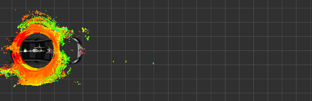
Figure 1: Point cloud of a Velodyne HDL64-S3D in dense fog.

In order to compare these different forms of lidar systems in adverse weather conditions, an easy and reproducible benchmark is needed. Within the European Union (EU) project aDverse wEather eNvironment Sensing systEm (DENSE), we present such a test procedure for state of the art lidar sensors and the results. Moreover, we show and evaluate disturbance patterns. All these results mark a baseline for upcoming developments in the project.

I-B Related Work

I-B1 Lidar characterization

In addition to theoretical characterization of lidar systems as in [7], experimental evaluation and especially benchmarks between different sensor technologies are very important. A first experimental study was already performed in 1991 by Hebert and Krothov [8]. They verified measurement models with experiments and quantized both range precision and angular precision. As soon as 2D laser scanners such as the Sick LMS 200 were commercially available, they were characterized by Ye and Borenstein [9] through extensive experimentation. A square target was precisely moved in front of the laser scanner in order to obtain insight into phenomena such as the range drift over time, the effect of the incidence angle and the mixed pixels problem. In 2008, a first assessment of four different laser range finders (Sick LMS200, Hokuyo URG-04LX, Ifm Effector O1D100 and Sick DT60) were performed [10]. This benchmark was extended in [11] where a total of 10 different range sensors were evaluated. In addition to characterization in the lab, measurements in underground environments showed the performance of these sensors in real environments.

I-B2 Influence of bad weather on lidar systems

When Peynot et al. recorded a dataset for an advanced perception system for autonomous vehicles in environmental conditions (dust, smoke and rain), they observed that dust particles in the air are detected by laser sensors and hide obstacles behind the dust cloud [12]. In [13], Rasshofer et al. theoretically investigated the influence of weather phenomena based on Mie’s theory in order to develop a novel electro-optical laser radar target simulator system. They verified their models with real world measurements in fog, rain and snow, however, these measurements rely on random weather conditions and cover only rough visibility differences. Ijaz et al. showed in [14] that the attenuation due to fog and smoke in a free space optical communication link are not wavelength dependent for visibilities less than 500 m and wavelengths in between 600-1500 nm. Their evaluations were performed in a very small laboratory controlled atmospheric chamber. Trickey et al. investigated the penetration performance of the Opal Lidar in dust, fog, snow whiteouts and smoke [5]. Dust and fog performances have been evaluated in an aerosol chamber while snow conditions and smoke were obtained in field tests. A very detailed inspection and discussion of two popular wavelengths for lidar systems, i.e. 905 nm and 1550 nm, was done by Wojtanowski et al. [15]. Recently, Hasirlioglu et al. studied the disturbances due to low ambient temperatures and exhaust gases [16]. Considering all these references [12, 13, 14, 5, 15, 16], it is clear that there is a huge impact from adverse weather on lidar systems. Some even have floated the idea to estimate the weather conditions by comparing lidar points in good weather and in adverse weather [17]. For autonomous driving in adverse weather, it is very important to gain even more insight into the degradation of lidar systems. This work presents a very detailed performance evaluation of four popular automotive lidar systems under defined weather conditions in a fog chamber. The size of the fog chamber allows us to set up a realistic street scenario and it is possible to generate fog with two different droplet distributions and change the visibility in very small steps.

II Tested laser scanners

TABLE I: Technical summary of the tested laser scanners. Differences between similar models are marked red.

Manufacturer	Velodyne	Ibeo
Model	HDL-64S2/S3D	LUX /LUX HD
Laser layers	64	4
Range [m]	50/120	50/200 30/120
Multiple echoes	1 2	3
Heavy duty	No	No Yes
Wavelength [nm]	905	905
Data rate [Hz]	5-20	12.5/25/50
Horiz. FOV [∘]	360	85
Horiz. resolution [∘]	0.0864-0.1728	0.125/0.25/0.5
Vert. FOV	26.33	3.2
Vert. spacing	$1/2$ to $1/3^{\circ}$	0.8
Embedded software	No	Yes
Distance accuracy [cm]	$\leq$2@1$\sigma$	4
Operating temp. [∘C]	-10 to 50 60	-40 to 85
Points per second	$\approx 1.3\times 10^{6}$ $\approx 2\times 10^{6}$	$\approx 44\times 10^{3}$

In this test, four state of the art laser scanners from Ibeo and Velodyne are compared with one another, i.e. Velodyne HDL-64S2, Velodyne HDL-64S3, Ibeo LUX and Ibeo LUX HD. A technical summary of these models can be found in Table I. Both Velodyne laser scanners S2 and S3 do not differ in their specifications. A 10 % reflective target is visible up to 50 m. A high reflective target with 80 % reflectivity is visible up to 120 m. However, the S2 is an older model and since scan quality has increased (Fig. 2).

S2	S2/S3D	S3D
long exp.	short exp.	long exp.

Figure 2: Captured laser intensities with a Raptor OWL-640 camera on a 50% dry reflective target. A short exposure was set to capture the scan pattern for the S3D and S2, which are equivalent. Longer exposure times illustrate the different scan qualities between the S2 and S3. Notice the increased uniformity for the S3D.

Primarily the intensity calibration was enhanced and is now stable across different scanning layers. The S3 generation is split into two subproducts: The Velodyne S3S and S3D. The S stands for single return and D for dual return. In our case, the dual return option is more interesting, as it is able to detect the strongest and last return from a laser pulse and transmit both to a host computer. As the bandwidth is limited to 1 Gigabit per second, the horizontal resolution is reduced by approximately 30 %. Counting both strongest and last returned points, the overall number of points increases from $\approx 1.3$ Mio. to $\approx 2$ Mio. points. We expect that the usage of multiple echoes will enable greater fog penetration.

Furthermore, both Ibeo scanners are technically similar because the Ibeo LUX HD is based on the Ibeo LUX. HD designates heavy duty because the LUX HD was originally developed for combine harvesters, where the environment is very dusty. The main difference is a modified lens and a tinted covering. The sensor was modified in order to enable more robust detections at close distances, as the laser scanners had to face a great deal of whirled-up dust. Due to the changes, the maximum viewing distance has been lowered. Both laser scanners offer four scanning rows and the same resolution.

In total, the Velodyne and Ibeo scanners differ quite a lot despite both having the same wavelength (905 nm) and mechanical beam steering. The Velodyne scanner offers a 360^∘ field of view (FOV), while the field of view of the Ibeo scanners is limited to 85^∘. Moreover, the resolution of the Velodyne sensors is several magnitudes larger and enables a more detailed environment perception. In addition, the Velodyne scanner is able to provide the intensity for each perceived point.

II-A Intensity calculation

For current automotive application, the measured intensity is becoming increasingly important. [18] reviews an overall calibration process and possible influences on intensity measures. In addition, four levels of intensity calibration are defined. It starts with level 0, where raw intensity measures are provided by a laser scanner and ends with level 3, where a rigorous calibration has been applied and the intensity measures are correct and identical across different systems. Level 0 calibration methods are provided by the laser scanner manufacturer and the produced output intensities are not comparable to other manufacturers.

The process of measuring the true intensity differs from each manufacturer and is proprietary, but this measuring process is crucial for a robust environment perception and can increase the robustness in adverse weather, as [19] and [20] show. Only the Velodyne scanners (S2 and S3D) provide a raw intensity measure (level 0), which will be analyzed for possible influences due to fog.

In [21], Velodyne claims to increase the capabilities in adverse weather, due to the usage of a digital signal processor which enables dynamically tuning the laser power if a clear object reflection is not obtained from a certain laser pulse. Both Velodyne S2 and S3D are able to apply this process automatically and to choose from eight power levels. The power level is set in an intelligent manner and enables different power levels for different reflective targets within one scan. The S3D models has the unique ability to set this parameter manually for all points and return the actual laser power for each laser point, however, at the expense of 3 bits meaning a loss of 1.4 cm depth resolution. Furthermore, the noise level can be set. The noise level describes the ground uncertainty floor for a detected signal from spurious light and thermal excitations. In this sense, the parameters will be tuned and an optimal performance point will be derived in Section IV-D.

In order to achieve a level 0 raw data point cloud the hardware inhomogeneity between each laser inside the Velodyne laser scanners has to be corrected. Each laser beam is collimated by an independent lens and driven by an independent laser diode. Therefore, the beam divergence is not uniform. Velodyne provides a factory-side calibration containing a slope $s$ and focal distance $f_{d}$ for each laser in order to correct the beam divergence. The raw intensity $I_{R}$ is corrected to $I_{C}$ with the know distance $d$ from the point measurement by

$$I_{C}=I_{R}+s\left|\left(f_{0}-\left(1-\frac{d}{\max(d)}\right)^{2}\right)\right|$$ (1)

where $f_{0}$ is given by

$$f_{0}=\left(1-\frac{f_{d}}{\text{scale}}\right)^{2}.$$ (2)

One has to keep in mind that beam divergence is worse if the laser beam is confronted with a scattering medium and more sophisticated methods can be defined for a known visibility. [22] offers a good introduction into the physics of scattering processes.

III Experiments

Well-defined weather conditions are essential for testing and comparing different sensors. To the authors’ best knowledge, the climate chamber of CEREMA in Clermont Ferrand (France) is the only one in Europe that is able to produce stable fog with a certain meteorological visual range $V$ in two different fog droplet distributions, i.e. radiation fog (small droplets) and advection fog (large droplets) [23]. The fog density is continuously controlled by a transmissometer that measures the atmospheric transmission factor $T$. As described in [23], the meteorological visual range $V$, also known as visibility, can be derived from $T$ as a more practical parameter to determine the fog density.

We set up a static scene as depicted in Fig. 3.

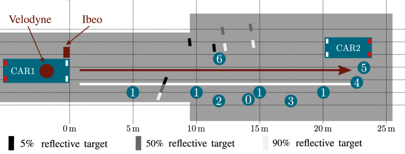
Figure 3: Experiment setup in the fog chamber.

The static scene contains many different targets, see Fig. 4: old exhaust pipe (0), reflector posts (1), differently pedestrian mannequins, i.e. child (2), woman (3), man (4), traffic sign (5), tire without rim (6), car (CAR2), road marking and multiple reflective targets.

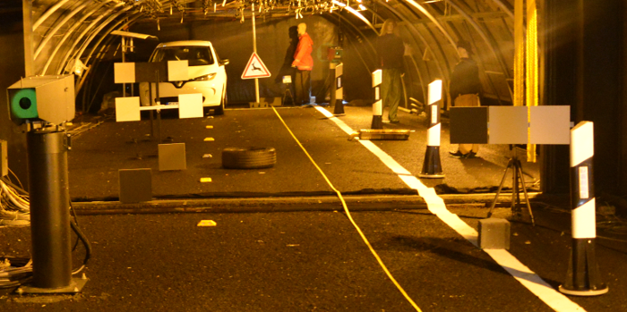
Figure 4: Experiment setup in the fog chamber.

The lidar sensors are placed at the beginning of the chamber where the test vehicle (CAR1) is located. The Velodyne sensors, i.e. HDL64-S2 and HDL64-S3D, are mounted on top of CAR1 while the Ibeo sensors, i.e. Lux and Lux HD, are mounted as they would be on a bumper on the left side of CAR1 at a height of approximately 0.9 m with a forward-looking field of view (see Fig. 3). The static scene is recorded under different fog densities and fog droplet distributions in order to investigate the influence of fog to the lidar performance. Because the Velodyne HDL64-S3D internal parameters laser output power and noise ground level can be varied, the influence of these parameters on measurements in adverse weather can be estimated.

		HDL64-S2	HDL64-S3 strongest	HDL64-S3 last
reference
$V=45\,\mathrm{m}$	radiation
	advection
$V=36\,\mathrm{m}$	radiation
	advection
$V=24\,\mathrm{m}$	radiation
	advection
$V=13\,\mathrm{m}$	radiation
	advection

Figure 5: Bird view of the Velodyne sensors for different fog types and fog densities. Color encodes the intensity.

IV Evaluation

	Ibeo LUX		Ibeo LUX HD
	advection	radiation	advection	radiation
reference
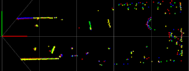
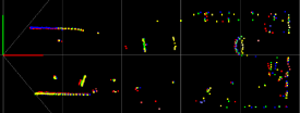
45 m
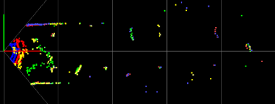
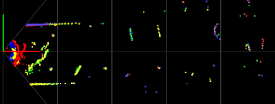
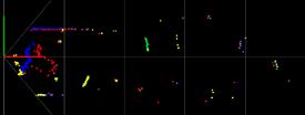
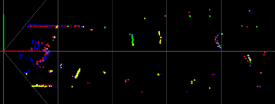
36 m
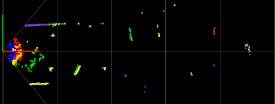
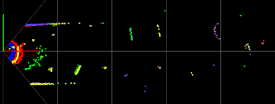
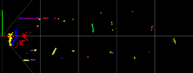
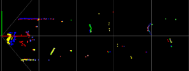
24 m
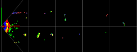
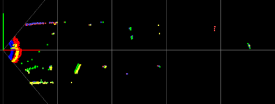
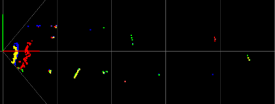
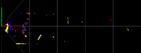
13 m

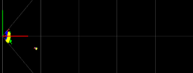
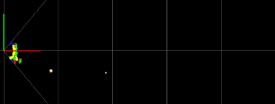
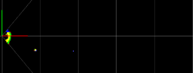
Figure 6: Bird’s-eye views of the Ibeo sensors for different fog types and fog densities. Color encodes the layer: layer 1 (red), layer 2 (blue), layer 3 (green), layer 4 (yellow).

IV-A Qualitative Evaluation

For a first impression of the lidar performance in fog, we qualitatively assess the bird’s-eye views in Fig. 5 and 6. Fig. 5 shows the bird’s-eye views for the strongest and last return for both the Velodyne HDL64-S2 and the HDL64-S3D. The colors encode the intensity. In general, it is obvious that fog impairs lidar performance heavily. The fog disturbance results in a cloud around the sensor, because the signal is reflected by fog droplets close to the car. This creates the need to filter such clutter points, drastically reducing the effective resolution. In the HDL64-S3D scans a constant red circle around the laser scanner is visible. Those points appear if the recorded echoes are below the noise level and are therefore projected to their default position. This can only be observed if the power return mode is activated, otherwise no point is returned. Moreover, the maximal viewing distance is limited by attenuation because the illumination power is limited and possible reflected signals vanish in the signal noise. The Velodyne HDL64-S3D delivers better results than the older model HDL64-S2. With respect to the bird’s-eye view, there is no visible difference between strongest and last return. For small visibilities around 13 m, all sensors suffer more in radiation fog than in advection fog. For higher visibilities the performance is equal or even better in radiation fog than in advection fog.

The bird’s-eye views for the Ibeo LUX and Ibeo LUX HD are illustrated in Fig. 6. The color coding indicates the corresponding layer, i.e. layer 1 = red, layer 2 = blue , layer 3 = green, layer 4 = yellow. As for the Velodyne sensors, fog reduces the maximal viewing distance heavily. By design, the Ibeo LUX HD contains less clutter than the Ibeo LUX. Starting from $V=36\,\mathrm{m}$, both Ibeo sensors are able to detect all targets in the experiment setup while the Velodyne sensors still have difficulties in larger distances. There is no difference visible between advection and radiation fog. Compared to the Velodyne sensors, the Ibeo sensors can perceive the license plate of the car and the traffic sign at a lower visibility starting from 24 m. As there is only a small difference between advection and radiation fog, we continue the following evaluation with only advection fog.

IV-B Maximum viewing distances

For a more detailed evaluation, a person successively moved three large well-calibrated Zenith Polymer diffuse reflective targets (50x50 cm) with reflectivities of 5%, 50% and 90% at a height of 0.9 m along the main viewing axis (see arrow in Fig. 3) in order to obtain the maximum viewing distance. The person and the target are well separated as the person holds the target 1.5 m away from their body with a pole. The maximum viewing distance is obtained by taking the distance from the last visible point on the targets. All sensors used their automatic algorithm to set the proper laser parameters. Due to the length of the chamber, the evaluation of the maximum viewing distance $d_{\text{max}}$ is limited. This limit differs in between the Ibeo and Velodyne sensors because of different mount points.

Figure 7: Maximum viewing distance comparison for all sensors in advection fog and reflective targets with 90% reflectivity.

Fig. 7 shows the maximum viewing distance vs meteorological visibility $V$ for all four sensors, based on the 90 % target. Since the targets are kept within the fog chamber and get wet as is common for objects in foggy conditions, they are not ideally diffusive reflective and a specular component can influence the measurements. In order to keep the targets dry, heating elements would be required and these would influence the fog homogeneity. Keeping the fog homogeneous is more important and as the targets are always directed towards the laser scanner, our results show an upper bound which can decrease for dry targets. Fig. 7 clearly illustrates that fog limits the maximum viewing distance $d_{\text{max}}$. At fog densities with $V<40\,\mathrm{m}$, $d_{\text{max}}$ is significantly less than 25 m. This is critical for driver safety as weather conditions can drop below 50 m visibility and the perceived depth from the laser scanners does not allow emergency stops on time. All sensors show equal performance within 0.5 m, despite the older Velodyne HDL64-S2. In this evaluation, there is almost no difference between strongest and last return. This is probably due to the specular component. Therefore, the last returned point is also the strongest.

IV-C Strongest Return vs. Last Return

Strongest and last return differ in modality. In general, the strongest return offers a more stable and accurate measure. But in adverse weather more received pulses grant a higher probability to get an actual object responses. This comparison points out the difference between different echoes in fog. In order to elaborate this difference, the static scenario is evaluated as follows: the point cloud 1.5 m in front of the car is binned in 122 depth slices of 0.25 m. Then, the number of points in each depth bin is obtained by averaging 100 point clouds.

Figure 8: Number of points in distance bins for clear weather and advection fog different visibilities $V$. For each fog density, the strongest and last echo is shown.

Fig. 8 shows the mean number of points obtained in each depth bin for different echoes. The power level is chosen automatically by the laser scanner and the noise level is set to the standard value 24. For clear weather, the strongest return and last return give the same point cloud which serves as ground truth reference. By increasing the fog density, it can be clearly seen that the number of points decreases and that the last return shows a larger overlap with the reference point cloud than the strongest return. The higher number of points compared to the ground truth is due to the clutter which is received at very close distance.

(a) Number of points

(b) Intensity

Figure 9: Evaluation for different laser power and noise levels in advection fog with different visibilities. The measurement shows the iteration over seven power levels (1-7) and for each power level the noise level is increased as follows: $\left[0,12,24,48,96,192,240\right]$.

IV-D Parameter Evaluation

As described before, the Velodyne HDL64-S3D offers the possibility to manually adjust the internal parameters laser output power and noise ground level. The power level can be set to an integer value in between 0 and 7. The noise level is a byte value, thus 0-255, which corresponds to the intensity value range. The measurement was iterated over the power levels $1-7$. For each power level the noise levels $\left[0,12,24,48,96,192,240\right]$ were set. Fig. 9 shows the number of points and intensities binned in depth slices over the measurement time in advection fog and for the last echo. As already mentioned, there is a clear correlation between the fog density and the number of points or rather the intensities. For all measurements, it can be seen that higher laser power guarantee a longer range while the noise level can adjust possible clutter.

Figure 10: Number of points achieved with a noise level of 0 plotted against the power level.

Fig. 10 gives the number of points vs power level at one single noise level 0 for different fog densities. For increased fog densities, the number of returned points increases with the laser output power. However, for clear conditions or light fog, high power levels make the laser prune to oversaturate the detector. Increasing the noise level means that more points in close distance can be observed and therefore the clutter points show a high intensity. This indicates that a depth-dependent noise level is required to filter out possible clutter points [19]. However, both parameters are restricted to either saturate the receiver if the laser power is too high, or to neglect many points if the noise level is too high.

Figure 11: Raw Intensities against distance of the HDL64-S3D on reflective targets (5 % and 90 %) for three different fog densities in advection fog.

IV-E Intensity Evaluation

The intensity values are of interest as they correspond directly to the measured signal peak amplitude. Therefore, the intensity also determines when the signal disappears. In this sense, it is interesting to determine which intensity is measured. In Fig. 11 the raw intensities for the 5 % and 90 % target against distance are plotted. The HDL64-S3D scanner is set to automatic laser power and the noise level is set to 24. As described in [24], intensity decreases exponentially due to attenuation. However, a fit to an exponential scattering model is not possible under the given confidence as the values jump when a less intense laser ring disappears from the target and is replaced by a higher intense laser ring. This inhomogeneity in between the laser rings of the HDL64-S3D can bee seen in Fig. 2 and is worse for the HDL64-S2. On average, 5 % reflective targets show a $\approx$ 20 % lower intensity than 90 % targets. It is worth to mention that the target disappears before reaching the minimum noise level.

V Conclusion and Outlook

In conclusion, the performance of all four state of the art laser scanners breaks down in fog. In direct comparison, only the older Velodyne HDL64-S2 is outperformed. Other sensors show similar performance, which is also due to the strict eye safety constraints lidar systems are facing within the near infrared (NIR) band to achieve laser class 1.

Manually adjusting internal parameters increases performance, e.g. increasing the laser output power for the HDL64-S3D increases range. Under adverse weather conditions, the sensors on average run only on level 5 out of 7 possible levels. The sensor algorithm may be confused by early high intense clutter responses which lead to a reduction of laser power. The authors assume that if any point is measured, the laser power is not increased further.

Overall in fog the maximal viewing distance is limited to a fraction of the clear weather capabilities. Below 40 m meteorological visibility, perception is limited to less than 25 m. Applying multiple echoes and adaptive noise levels increases performance in total by a magnitude of a few meters. But this is far away from reliable perception in dense foggy conditions. If this problem is not solved, autonomous driving will be limited to level four.

Therefore, intense research is needed to adapt lidar solutions from the military or airborne sector to cost sensitive and scalable laser scanners in the SWIR region. Otherwise, the transition to other technologies is interesting, e.g. gated imaging. For example, Goodrich and Brightway Vision provide gated cameras which work better under adverse weather but offer lower depth accuracy [25].

Further sensor tests have to be applied in order to monitor upcoming adverse weather systems and their improvements. This test provides a benchmark for current sensors and creates an awareness for sensor development. These findings are also interesting for upcoming raw data sensor fusion object detection systems like in [26]. Such methods rely purely on lidar data as proposal method and are therefore prone to failure with current lidar sensors in fog.

References

- [1] I. Olshansky, Y. Buda, and A. Lipson, “Road surface reflectivity detection by lidar sensor,” US Patent US9 453 941B2, Sep 27, 2016.
- [2] C. Boehlau and J. Hipp, “Optoelectronic detection device,” WO Patent WO2 004 036 245A2, Apr 29, 2004.
- [3] D. Hall, “High definition lidar system,” US Patent US20 110 216 304A1, Sep 8, 2011.
- [4] H. Urey, S. Holmstrom, and U. Baran, “MEMS laser scanners: a review,” Journal of Microelectromechanical Systems, vol. 23, no. 2, pp. 259–275, Apr 2014.
- [5] E. Trickey, P. Church, and X. Cao, “Characterization of the OPAL obscurant penetrating LiDAR in various degraded visual environments,” Proc. SPIE, vol. 8737, 2013.
- [6] J. M. Xiaoying Cao, Philip Church, “Characterization of the opal lidar under controlled obscurant conditions,” Proc. SPIE, vol. 9839, 2016.
- [7] W. K. Pratt, Laser Communication Systems. Wiley, 1969.
- [8] M. Hebert and E. Krotkov, “3D measurements from imaging laser radars: how good are they?” Image and Vision Computing, vol. 10, no. 3, pp. 170–178, 1992.
- [9] C. Ye and J. Borenstein, “Characterization of a 2D laser scanner for mobile robot obstacle negotiation,” in IEEE Int. Conf. on Robotics and Automation, vol. 3, no. May, 2002, pp. 2512–2518.
- [10] J. Pascoal, L. Marques, and A. T. De Almeida, “Assessment of laser range finders in risky environments,” IEEE/RSJ Int. Conf. on Intelligent Robots and Systems, pp. 3533–3538, 2008.
- [11] U. Wong, A. Morris, C. Lea, J. Lee, C. Whittaker, B. Garney, and R. Whittaker, “Comparative evaluation of range sensing technologies for underground void modeling,” in IEEE/RSJ Int. Conf. on Intelligent Robots and Systems, Sep 2011, pp. 3816–3823.
- [12] T. Peynot, J. Underwood, and S. Scheding, “Towards reliable perception for unmanned ground vehicles in challenging conditions,” in IEEE/RSJ Int. Conf. on Intelligent Robots and Systems, 2009, pp. 1170–1176.
- [13] R. H. Rasshofer, M. Spies, and H. Spies, “Influences of weather phenomena on automotive laser radar systems,” Advances in Radio Science, vol. 9, pp. 49–60, 2011.
- [14] M. Ijaz, Z. Ghassemlooy, H. Le-Minh, S. Rajbhandari, and J. Perez, “Analysis of Fog and Smoke Attenuation in a Free Space Optical Communication Link under Controlled Laboratory Conditions,” Int. Workshop Optical Wireless Communications, no. 1, pp. 1–3, 2012.
- [15] J. Wojtanowski, M. Zygmunt, Z. Mierczyk, and M. Muzal, “Comparison of 905 nm and 1550 nm semiconductor laser rangefinders’ performance deterioration due to adverse environmental conditions,” Opto-Electronics Review, 2014.
- [16] S. Hasirlioglu, A. Riener, W. Ruber, and P. Wintersberger, “Effects of exhaust gases on laser scanner data quality at low ambient temperatures,” IEEE Intelligent Vehicle Symposium, pp. 1708–1713, 2017.
- [17] J. Zhu, D. Dolgov, and D. Ferguson, “Methods and systems for detecting weather conditions including fog using vehicle onboard sensors,” US Patent US8 983 705B2, Mar 17, 2015.
- [18] A. G. Kashani, M. J. Olsen, C. E. Parrish, and N. Wilson, “A review of lidar radiometric processing: From ad hoc intensity correction to rigorous radiometric calibration,” Sensors, vol. 15, no. 11, 2015.
- [19] P. Kramper and T. Muensterer, “A method for determination of a plurality of distinct echo pulses in order to provide distance measurements by an active 3d sensor,” WO Patent WO2 016 173 712A1, Nov 3, 2016.
- [20] A. Ullrich and R. Reichert, “High resolution laser scanner with waveform digitization for subsequent full waveform analysis,” Proc. SPIE, vol. 5791, 2005.
- [21] D. Hall, “High definition lidar system,” US Patent US7 969 558B2, Jun 28, 2011.
- [22] B. Bruce and P. Robert, Dynamic light scattering. Courier Dover Publications, 2000.
- [23] M. Colomb, K. Hirech, P. André, J. Boreux, P. Lacôte, and J. Dufour, “An innovative artificial fog production device improved in the european project fog,” Atmospheric Research, vol. 87, no. 3–4, pp. 242–251, 2008.
- [24] S. G. Narasimhan and S. K. Nayar, “Vision and the atmosphere,” Int. Journal of Computer Vision, vol. 48, no. 3, pp. 233–254, Jul 2002.
- [25] M. Bijelic, T. Gruber, and W. Ritter, “Benchmarking Image Sensors Under Adverse Weather Conditions for Autonomous Driving,” in IEEE Intelligent Vehicle Symposium, 2018.
- [26] X. Chen, H. Ma, J. Wan, B. Li, and T. Xia, “Multi-view 3d object detection network for autonomous driving,” in Conf. on Computer Vision and Pattern Recognition, 2017.