Floquet states in dissipative open quantum systems

Abstract

We theoretically investigate basic properties of nonequilibrium steady states of periodically-driven open quantum systems based on the full solution of the Maxwell-Bloch equation. In a resonantly driving condition, we find that the transverse relaxation, also known as decoherence, significantly destructs the formation of Floquet states while the longitudinal relaxation does not directly affect it. Furthermore, by evaluating the quasienergy spectrum of the nonequilibrium steady states, we demonstrate that the Rabi splitting can be observed as long as the decoherence time is as short as one third of the Rabi-cycle. Moreover, we find that Floquet states can be formed even under significant dissipation when the decoherence time is substantially shorter than the cycle of driving, once the driving field strength becomes strong enough. In an off-resonant condition, we demonstrate that the Floquet states can be realized even in weak field regimes because the system is not excited and the decoherence mechanism is not activated. Once the field strength becomes strong enough, the system can be excited by nonlinear processes and the decoherence process becomes active. As a result, the Floquet states are significantly disturbed by the environment even in the off-resonant condition. Thus, we show here that the suppression of heating is a key condition for the realization of Floquet states in both on and off-resonant conditions not only because it prevents material damage but also because it contributes to preserving coherence.

I Introduction

Nonlinear interaction of strong light with matter is an important subject from both fundamental and technological points of view and has been intensively investigated for a long time Franken et al. (1961); Butcher and Cotter (1990); Boyd (2008); Mourou et al. (2012); Flick et al. (2017); Ruggenthaler et al. (2018). Laser fields can directly couple with electrons in matter and induce nonequilibrium electron dynamics. Thus, strong laser fields can be employed to control the electronic properties and functionalities of materials Krausz and Ivanov (2009); Krausz and Stockman (2014); Basov et al. (2017). In the ultrafast regime, light-induced electron dynamics in solids within sub-femtosecond time-scale have been intensively investigated towards petahertz electronics Schiffrin et al. (2012); Schultze et al. (2012, 2014); Lucchini et al. (2016); Mashiko et al. (2016); Schlaepfer et al. (2018); Siegrist et al. (2019); Volkov et al. (2019). In addition, strong light may also couple with phonons in solids and renormalize electron-phonon coupling, triggering light-induced superconductivity Fausti et al. (2011); Mitrano et al. (2016). In these light-induced phenomena, target systems are actively driven by light. Therefore, substantial energy transfer from light to matter is expected Sommer et al. (2016). In most cases, the systems of interest are not isolated but are coupled to their surrounding environment. Thus, a part of the transferred energy is dissipated to the environment. Moreover, through the interaction with the environment, coherence of light-induced dynamics can be lost. Therefore, proper understanding of light-driven dynamics in a dissipative environment is indispensable towards realization of optical-control of realistic systems.

Nonequilibrium dynamics of periodically-driven non-dissipative systems has been intensively investigated with Floquet theory, and various interesting properties of the driven systems have been discussed such as the emergence of new topological states Oka and Aoki (2009), the dynamical localization Dunlap and Kenkre (1986); Großmann and Hänggi (1992), among others Eckardt (2017); Shin et al. (2018); Giovannini and Hübener (2019); Claassen et al. (2019). Theoretical investigation of periodically-driven systems has been further extended to dissipative systems, or namely, open quantum systems Kohler et al. (1997); Grifoni and Hänggi (1998); Restrepo et al. (2016); Hartmann et al. (2017), and the effects of the dissipative environment have been discussed in various aspects such as realization of Floquet-Gibbs state Kohn (2001); Shirai et al. (2015, 2016); Engelhardt et al. (2019), the asymptotic states under the memory-effect Magazzù et al. (2017, 2018), and topological properties Dehghani et al. (2014, 2015). Furthermore, experimental studies have been conducted for strongly driven quantum systems Wilson et al. (2007); Deng et al. (2015); Magazzù et al. (2018), and the Floquet-Bloch states have been experimentally observed as the Rabi-splitting in the angular-resolved photo-electron spectroscopy (ARPES) in extended systems Wang et al. (2013). Recently, the light-induced anomalous Hall effect in graphene has been experimentally observed McIver et al. (2019), originating from population effects on top of the realization of Floquet states subjected to substantial dissipation Sato et al. (2019a, b).

Optical-control of materials based on Floquet engineering has been attracting great interest ranging from light-induced topological phase transitions Oka and Aoki (2009); Hübener et al. (2017) to optical control of chiral superconductors Claassen et al. (2019). However, the realization of Floquet states and the control of their population are highly nontrivial tasks in a dissipative environment Hone et al. (2009); Seetharam et al. (2015). In this work, we theoretically investigate basic properties of periodically-driven open-quantum systems with Maxwell-Bloch equation Arecchi and Bonifacio (1965); Meier et al. (2007), which may be the simplest model for driven open-quantum systems, and provide an insight into the realization of Floquet states in such systems, addressing the following open questions: Which kind of relaxation mechanism affects the formation of Floquet states, and which does not? How long is coherence required to persist to realize Floquet states? Can Floquet states be formed even under a significant dissipation, e.g. when the relaxation time is shorter than a driving period?

The paper is organized as follows: In Sec. II we first describe the Maxwell-Bloch equation and several equivalent descriptions of open quantum systems. Then, we introduce basic quantities of nonequilibrium steady states, Floquet fidelity and quasienergy spectrum, which will be investigated in the following sections. In Sec. III we investigate the properties of the nonequilibrium steady state in both resonant and off-resonant conditions. Finally, our findings are summarized in Sec. IV.

II Method

Here, we describe theoretical methods to investigate basic properties of nonequilibrium steady states of open quantum systems under a periodic driving. First, we introduce the Maxwell-Bloch equation, where time-evolution of a density matrix of a two-level system under a periodic driving is described with relaxation time approximation. Then, we revisit equivalent descriptions of the open-quantum system with the Lindblad equation and the stochastic Schrödinger equation. Finally, we introduce two quantities to study nonequilibrium steady states; Quasienergy spectrum of driven open-quantum systems and Floquet fidelity Sato et al. (2019a, b).

II.1 Equation of motion of driven open-quantum systems

In order to get a microscopic understanding of the nonequilibrium dynamics of open quantum systems, we consider a two-level driven system in dissipative environment based on the Maxwell-Bloch equation. For detailed analysis of the nonequilibrium system, we further revisit equivalent descriptions in different forms.

II.1.1 Maxwell-Bloch equation

We first revisit the description of nonequilibrium dynamics of a two-level system based on Maxwell-Bloch equation Arecchi and Bonifacio (1965), which can be seen as the simplest form of the semiconductor Bloch equation and has been used to develop microscopic insight into the driven dynamics of dissipative systems Meier et al. (2007). Note that the semiconductor Bloch equation with the simple relaxation time approximation Meier et al. (1994) has been widely employed in studies on various phenomena of nonlinear light-matter interactions such as the attosecond electron dynamics Moulet et al. (2017), the high-order harmonic generation from solids Luu et al. (2015); Yoshikawa et al. (2017) and the light-induced anomalous Hall effect Sato et al. (2019a). Furthermore, it has been demonstrated that the simple approximation already performs excellently when compared to the experimental results. Based on this fact, here we employ the simplest relaxation time approximation in order to clarify the primary role of the dissipation in driven quantum systems.

The time propagation of the system is described by the following quantum master equation

$$\frac{d}{dt}\rho(t)=\frac{\left[H(t),\rho(t)\right]}{i\hbar}+\hat{D}\left[\rho(t)\right],$$ (1)

where $\rho(t)$ is the density matrix of the two-level system, $H(t)$ is the Hamiltonian, and $\hat{D}\left[\rho(t)\right]$ is the relaxation operator. The Hamiltonian of the two-level system is given by

$$H(t)=\frac{\Delta}{2}\sigma_{z}+F_{0}\sin(\Omega t)\sigma_{x},$$ (2)

where $\sigma_{i}$ are Pauli matrices, $\Delta$ is the gap of the two-level system, $F_{0}$ is the amplitude of an external field, and $\Omega$ is its frequency. Furthermore, the dissipation operator is constructed with the relaxation time approximation, where the relaxation is simply treated as simpe exponential decays Meier et al. (1994), as

$$\hat{D}\left[\rho(t)\right]=\left(\begin{array}[]{cc}-\frac{\rho_{ee}(t)}{T_{1}}&-\frac{\rho_{eg}(t)}{T_{2}}\\ -\frac{\rho_{ge}(t)}{T_{2}}&-\frac{\rho_{gg}(t)-1}{T_{1}}\end{array}\right),$$ (5)

where $\rho_{ij}(t)$ is a matrix element of the density matrix, $\langle i|\rho(t)|j\rangle$, with the eigenbasis of the subsystem Hamiltonian, $\Delta\sigma_{z}/2$; $|g\rangle=(0,1)^{\dagger}$ corresponds to the ground state, while $|e\rangle=(1,0)^{\dagger}$ corresponds to the excited state. While the longitudinal relaxation time $T_{1}$ corresponds to the population decay constant from the excited state $|e\rangle$ to the ground state $|g\rangle$, the transverse relaxation time $T_{2}$ corresponds to the decay constant for coherence. Thus, in this work, we shall call $T_{2}$ decoherence time.

II.1.2 Lindblad equation

To smoothly connect the Maxwell-Bloch equation to the equivalent stochastic Schrödinger equation approach Breuer et al. (2002); Lidar (2019), which will be used to introduce the quasienergy spectrum of the driven system later, here we revisit the relation between the Maxwell-Bloch equation and the Lindblad equation Breuer et al. (2002); Lidar (2019). The quantum master equation (1) with the relaxation time approximation (5) can be equivalently expressed in the following Lindblad form

$$\frac{d}{dt}\rho(t) = \frac{\left[H(t),\rho(t)\right]}{i\hbar}$$ (6)

$$+\sum^{2}_{\alpha=1}\gamma_{\alpha}\left(L_{\alpha}\rho(t)L^{\dagger}_{\alpha}-\frac{1}{2}\left\{L^{\dagger}_{\alpha}L_{\alpha},\rho(t)\right\}\right)$$

by employing the two Lindblad operators,

$$L_{1} = \sigma_{x}-i\sigma_{y},$$ (7)

$$L_{2} = -\sigma_{z}.$$ (8)

Here, the anticommutator is defined as $\{A,B\}=AB+BA$. The scattering rate $\gamma_{\alpha}$ in the Lindblad equation (6) and the relaxation time $T_{i}$ in the Maxwell-Bloch equation (1) have the following relations,

$$\frac{1}{T_{1}} = \gamma_{1},$$ (9)

$$\frac{1}{T_{2}} = \frac{\gamma_{1}}{2}+2\gamma_{2}.$$ (10)

Note that the Lindblad master equation (6) is invariant under the arbitrary phase multiplication, $L_{i}\rightarrow e^{i\theta}L_{i}$. Nevertheless, we explicitly choose the form of the Lindblad operator, especially for, $L_{2}$ so that the environment scatters only the excited state $|e\rangle$ but the ground state $|g\rangle$ is not scattered in the following Stochastic approach. Preventing scattering of the ground-state also avoids unphysical modification of the quasienergy spectrum of the undriven system that would occur otherwise.

II.1.3 Stochastic Schrödinger equation approach

The Lindblad equation (6) for the density matrix propagation can be equivalently described by a stochastic approach based on non-Hermitian Schrödinger equation for the wavefunction propagation Breuer et al. (2002); Lidar (2019). Therefore, the Maxwell-Bloch equation can be equivalently evaluated with the stochastic Schrödinger equation approach.

For later convenience, we revisit this stochastic trajectory approach Breuer et al. (2002); Lidar (2019). To introduce the wavefunction propagator, we rewrite the Lindblad equation (6) as

$$\frac{d}{dt}\rho(t)=\frac{\left[H_{c}(t),\rho(t)\right]}{i\hbar}+\sum^{2}_{\alpha=1}\gamma_{\alpha}L_{\alpha}\rho(t)L^{\dagger}_{\alpha}$$ (11)

with the conditional Hamiltonian defined as

$$H_{c}(t)\equiv H(t)-\frac{i\hbar}{2}\sum^{2}_{\alpha=1}\gamma_{\alpha}L^{\dagger}_{\alpha}L_{\alpha}.$$ (12)

The time-evolution of the density matrix $\rho(t)$ obeying the Lindblad equation (6) can be obtained by propagating the non-Hermitian Schrödinger equation, $i\hbar d/dt|\tilde{\psi}(t)\rangle=H_{c}(t)|\tilde{\psi}(t)\rangle$, with stochastic quantum jumps that occur at a given time step. The probability of the stochastic quantum jump is evaluated from the norm of the wavefunction, $\langle\tilde{\psi}(\tau)|\tilde{\psi}(\tau)\rangle$. In practical calculations, we employ the the following algorithm. For simplicity, here we assume that the initial density matrix $\rho(0)$ is a pure state: $\rho(0)=|\tilde{\psi}(0)\rangle\langle\tilde{\psi}(0)|$.

(i)

Set the initial wavefunction to the initial pure state $|\tilde{\psi}(0)\rangle$.

(ii)

Propagate the wavefunction $|\tilde{\psi}(t)\rangle$ by the non-Hermitian conditional Hamiltonian $H_{c}(t)$;

$$i\hbar\frac{d}{dt}|\tilde{\psi}(t)\rangle=H_{c}(t)|\tilde{\psi}(t)\rangle.$$ (13)

(iii)

Perform quantum jump at $t_{j}+\tau$ after time $\tau$ since the last jump at $t_{j}$ with probability $p=\langle\tilde{\psi}(t_{j}+\tau)|\tilde{\psi}(t_{j}+\tau)\rangle$;

$$|\tilde{\psi}(t_{j}+\tau)\rangle\mapsto\frac{L_{\alpha}|\tilde{\psi}(t_{j}+\tau)\rangle}{\sqrt{\langle\tilde{\psi}(t_{j}+\tau)|\tilde{\psi}(t_{j}+\tau)\rangle}},$$ (14)

where the index $\alpha$ is chosen with probability

$$p_{\alpha}=\frac{\gamma_{\alpha}\langle\tilde{\psi}(t_{j}+\tau)|L^{\dagger}_{\alpha}L_{\alpha}|\tilde{\psi}(t_{j}+\tau)\rangle}{\sum_{\beta}\gamma_{\beta}\langle\tilde{\psi}(t_{j}+\tau)|L^{\dagger}_{\beta}L_{\beta}|\tilde{\psi}(t_{j}+\tau)\rangle}.$$ (15)

(iv)

Repeat the steps (ii) and (iii) until the simulation time $t$ reaches the final time of the simulation $t_{f}$.

(v)

Repeat the above stochastic procedures and evaluate the density matrix as the statistical average from the stochastic trajectories as

$$\rho(t)\approx\left<\frac{|\tilde{\psi}(t)\rangle\langle\tilde{\psi}(t)|}{\langle\tilde{\psi}(t)|\tilde{\psi}(t)\rangle}\right>_{average}.$$ (16)

In the limit of large number of trajectories, it can be demonstrated Breuer et al. (2002); Lidar (2019) that the statistical average converges to the solution of the Lindblad equation (6).

Note that the expectation value of an operator $\hat{A}$ can be evaluated as the statistical average of the corresponding expectation value of the stochastic wavefunctions as

$$\langle A\rangle = \mathrm{Tr}\left[\hat{A}\rho(t)\right]\approx\mathrm{Tr}\left[\hat{A}\left<\frac{|\tilde{\psi}(t)\rangle\langle\tilde{\psi}(t)|}{\langle\tilde{\psi}(t)|\tilde{\psi}(t)\rangle}\right>_{average}\right]$$ (17)

$$= \left<\frac{\langle\tilde{\psi}(t)|\hat{A}|\tilde{\psi}(t)\rangle}{\langle\tilde{\psi}(t)|\tilde{\psi}(t)\rangle}\right>_{average}.$$

II.2 Quasi-energy spectrum of driven open-quantum systems

Here, we introduce a computational scheme to evaluate a quasienergy spectrum of driven systems. The scheme is inspired by what is done in the modeling of photoelectron spectroscopy (PES), which is widely used to investigate equilibrium quasiparticle energy spectra as well as those of driven systems Cardona and Ley (1978); Damascelli et al. (2003); Wang et al. (2013); Giovannini and Hübener (2019).

First, we describe the method to compute the quasienergy spectrum of closed driven systems. Later, we will extend it to open quantum systems based on the above stochastic Schrödinger equation approach. Here, we consider a two level system described by the following Schrödinger equation,

$$i\hbar\frac{d}{dt}|\psi(t)\rangle = H(t)|\psi(t)\rangle$$ (18)

$$= \left[\frac{\Delta}{2}\sigma_{z}+F(t)\sigma_{x}\right]|\psi(t)\rangle,$$

where $F(t)$ is a time-dependent external field. In order to investigate the quasienergy spectrum of the driven system, we introduce theoretical detector states, $|\epsilon\rangle$, associated with each detected energy $\epsilon$. By embedding these theoretical detector states into the original Hilbert space of the two-level system, we reconstruct the Hamiltonian of the full system as

$$H^{E}(t)= H(t)+\int^{\infty}_{-\infty}d\epsilon|\epsilon\rangle\epsilon\langle\epsilon|$$ (19)

$$+ v(t)\int^{\infty}_{-\infty}d\epsilon\bigg{(}|\epsilon\rangle\langle i|+|i\rangle\langle\epsilon|\bigg{)},$$

where the first term is the original Hamiltonian of the system that is being probed $H(t)$, the second term is the Hamiltonian of the embedded detector states $|\epsilon\rangle$, and the last term is the interaction between the system of interest and the theoretical detector states via a probe field $v(t)$. In the interaction Hamiltonian, $|i\rangle$ denotes a state of the original system that we would like to probe, and we set it to the ground state $|i\rangle=|g\rangle$. Furthermore, we employ the following form for the probe field,

$$v(t)=f(t)\sin\left(\omega t\right),$$ (20)

where $\omega$ is the driving frequency of the probe perturbation, and $f(t)$ is an envelope function. Assuming the probe field is weak enough, the solution of the Schrödinger equation of the full system, $i\hbar d/dt|\psi^{E}(t)\rangle=H^{E}(t)|\psi^{E}(t)\rangle$ can be approximated by

$$|\psi^{E}(t)\rangle\approx|\psi(t)\rangle+\int^{\infty}_{-\infty}d\epsilon\,c(\epsilon,t)e^{-i\frac{\epsilon}{\hbar}t}|\epsilon\rangle,$$ (21)

where $|\psi(t)\rangle$ is the solution of the Schrödinger equation of the original system, Eq. (18), and $c(\epsilon,t)$ is an expansion coefficient of the theoretical detector state $|\epsilon\rangle$. Employing the rotating wave approximation, the equation of motion for the coefficient $c(\epsilon,t)$ can be approximated as

$$\dot{c}(\epsilon,t)=\frac{f(t)}{2}\langle i|\psi(t)\rangle e^{i\frac{\epsilon-\omega}{\hbar}t}.$$ (22)

Thus, the population of the detector state $|\epsilon\rangle$ after the probe perturbation $v(t)$ can be evaluated as

$$n^{pop}(\epsilon):=\left|c(\epsilon,t=\infty)\right|^{2}=\left|\int^{\infty}_{-\infty}dt\frac{f(t)}{2}\langle i|\psi(t)\rangle e^{i\frac{\epsilon-\omega}{\hbar}t}\right|^{2}.$$

(23)

The population distribution at the detector reflects the quasienergy structure of the closed quantum system described by the Hamiltonian $H(t)$ as the conventional photoelectron spectroscopy does Cardona and Ley (1978); Damascelli et al. (2003); Wang et al. (2013); Giovannini and Hübener (2019).

We further extend this numerical PES scheme to open quantum systems. Inspired by a fact that the expectation value of an observable can be evaluated as the ensemble average of stochastic trajectories with Eq. (17), we evaluate the quasienergy spectrum of open quantum systems as the ensemble average of the spectrum of each trajectory. In practice, the population of the detector states in the case of open quantum systems is computed as the statistical average of stochastic trajectories,

$$n^{pop}(\epsilon)=\left<\left|\int^{\infty}_{-\infty}dt\frac{f(t)}{2}\frac{\langle i|\tilde{\psi}(t)\rangle}{\sqrt{\langle\tilde{\psi}(t)|\tilde{\psi}(t)\rangle}}e^{i\frac{\epsilon-\omega}{\hbar}t}\right|^{2}\right>_{average}.$$

(24)

Assuming the quasienergy structure is mapped to the population distribution of the detector states, $n^{pop}(\epsilon)$, by a single photon absorption with the energy of $\hbar\omega$, the quasienergy spectrum $A^{Q}(E_{Q})$ as a function of energy $E_{Q}$ can be evaluated as $A^{Q}(E_{q})\sim n^{pop}(E_{Q}+\hbar\omega)$.

II.3 Floquet fidelity

Here, we introduce a measure to quantify the similarity of nonequilibrium steady states under periodic driving fields and the corresponding Floquet states. We shall call it Floquet fidelity Sato et al. (2019a, b).

Floquet states $|\psi_{F,a}(t)\rangle$ are defined as solutions of the time-dependent Schrödinger equation with a time-periodic Hamiltonian, $id/dt|\psi_{F,a}(t)\rangle=H(t)|\psi_{F,a}(t)\rangle$, with the following form:

$$|\psi_{F,a}(t)\rangle=e^{-i\frac{\epsilon_{F,a}}{\hbar}t}|u_{F,a}(t)\rangle,$$ (25)

where $|u_{F,a}(t)\rangle$ has the same time-period as the Hamiltonian, $H(t)$, and $\epsilon_{F,a}$ is the Floquet quasienergy. As Floquet states are defined as the solutions of the time-dependent Schrödinger equation, they are not necessarily solutions of the quantum master equation (1). Nevertheless, nonequilibrium steady states of open quantum systems may show some signatures based on the corresponding Floquet states under certain conditions Kohn (2001); Shirai et al. (2015, 2016).

To introduce the Floquet fidelity, we first consider the eigenvalue decomposition of the density matrix in a nonequilibrium steady state as,

$$\rho(t)=\sum_{a}\lambda_{a}(t)|NO_{a}(t)\rangle\langle NO_{a}(t)|,$$ (26)

where $\lambda_{a}(t)$ is an eigenvalue and $|NO_{a}(t)\rangle$ is the corresponding eigenvector. Since the density matrix of the nonequilibrium steady state has the time-periodicity of the Hamiltonian, $\rho(t)=\rho(t+2\pi/\Omega)$, the eigenvalues and the eigenvectors may have the same periodicity, $\lambda_{a}(t)=\lambda_{a}(t+2\pi/\Omega)$ and $|NO_{a}(t)\rangle=|NO_{a}(t+2\pi/\Omega)\rangle$. These eigenvectors of the one-body reduced density matrix are known as natural orbitals Löwdin (1955), and the eigenvalues can be interpreted as their occupations. By construction of the natural orbitals, the expectation value of an observable $\hat{A}$ can be evaluated as the sum of the expectation value of each natural orbital with the occupation weight as

$$\langle A\rangle = \mathrm{Tr}\left\{\hat{A}\rho(t)\right\}$$ (27)

$$= \sum_{a}\lambda_{a}(t)\langle NO_{a}(t)|\hat{A}|NO_{a}(t)\rangle.$$

Therefore, the natural orbitals can be seen as very accurate representative single-particle states of the system. Based on this fact, we quantify the similarity of the nonequilibrium steady state and the Floquet states by the similarity of the corresponding natural orbitals and the Floquet states.

In practice, to define the similarity, we first introduce a Floquet fidelity matrix $F$ Sato et al. (2019a) whose matrix elements $F_{ij}$ are defined as the cycle average of the squared overlap of the $i$-th natural orbital and the $j$-th Floquet state as

$$F_{ij}=\frac{1}{T}\int^{T}_{0}dt\left|\langle NO_{i}(t)|\psi_{F,j}(t)\rangle\right|^{2},$$ (28)

where $T$ is the time-period of the Hamiltonian, $T=2\pi/\Omega$. Then, the Floquet fidelity $S_{F}$ is defined as the absolute value of the determinant of the Floquet fidelity matrix, $S_{F}=|\mathrm{det}F|$. The Floquet fidelity takes the maximum value of one only if all the natural orbitals have identical Floquet states. Therefore, if the Floquet fidelity is one, the Floquet states diagonalize the density matrix. In general, $0\leq S_{F}\leq 1$.

III Results

III.1 Resonant driving

We first investigate the nonequilibrium steady state of the two-level system under the periodic driving in the resonant condition, $\hbar\Omega=\Delta$. To realize the nonequilibrium steady state, we perform sufficiently long real-time propagation by solving the Maxwell-Bloch equation (1). Here, the initial condition is set to the ground state, $\rho(t=0)=|g\rangle\langle g|$.

Figure 1 shows the population of the excited state, $\rho_{ee}(t)=\langle e|\rho(t)|e\rangle$, of the two-level system as a function of time for different field strength, $F_{0}$. Here, both the relaxation times, $T_{1}$ and $T_{2}$, are set to $30\hbar/\Delta$ in order to investigate the dynamics under a relatively weak-relaxation condition, $T_{1},T_{2}\gg\hbar/\Delta$. At the initial time $(t=0)$, the excited population is zero as the initial state is set to the ground state $|g\rangle$. As seen from the figure, the excited population $\rho_{ee}(t)$ asymptotically reaches dynamics, which has the same time-periodicity as the external field $T$, in the long propagation limit for each field strength. In contrast, one sees that oscillatory features that have longer periodicity than $T$ are observed in the stronger field cases, and the periods of the oscillation depend on the field strength. The period of the oscillatory feature is close to that of the Rabi oscillation, $T_{R}=2\pi/\Omega_{R}$, where $\Omega_{R}$ is the Rabi frequency, $\Omega_{R}=F_{0}/\hbar$. Thus, these oscillatory features can be understood as the Rabi oscillation with damping due to the dissipation. We note that, as seen from Fig. 1, the timescale of approaching the steady state does not significantly depend on the field strength, $F_{0}$. Because the lower bound of $T_{1}$ is determined by $T_{2}$ as $T_{1}\geq T_{2}/2$, $T_{1}$ cannot be the relevant timescale independently. Thus, the relevant timescale of approaching the steady state is approximately determined by the decoherence time, $T_{2}$.

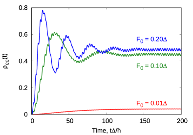
Figure 1: Population dynamics of the driven two-level system with dissipation under resonant driving ($\hbar\Omega=\Delta$) with different field strength $F_{0}$. The relaxation times, $T_{1}$ and $T_{2}$, are set to $30\hbar/\Delta$.

Now we turn to studying the basic properties of the nonequilibrium steady state, employing the Floquet fidelity, $S_{F}$. Figure 2 shows the computed Floquet fidelity of the nonequilibrium steady state as a function of driving field strength $F_{0}$. The results with different relaxation conditions are shown in the figure. The general feature is that, while the Floquet fidelity $S_{F}$ becomes zero in the weak field limit, $S_{F}$ asymptotically reaches unity in the strong field limit. This fact indicates that the Floquet states are significantly destructed by the dissipation in the weak field regime. In contrast, in the strong field regime, the contribution from the external driving field overcomes the dissipation effect, and the Floquet states are stabilized.

In Fig. 2, squares (purple), up-pointing triangles (red), and circles (green) show the computed Floquet fidelity $S_{F}$ with the same longitudinal relaxation time $T_{1}=30\hbar/\Delta$ but with different decoherence time $T_{2}$. Comparing these results, one sees that the Floquet fidelity becomes smaller when the decoherence time $T_{2}$ becomes shorter. This fact indicates that the coherence plays an important role to form the Floquet states, and the decoherence is a source of the destruction of the Floquet states. In contrast, in Fig. 2, up-pointing triangles (red) and down-pointing triangles (blue) show the Floquet fidelity with the same decoherence time $T_{2}=30\hbar/\Delta$ but different longitudinal relaxation time $T_{1}$. Despite the significant difference of the longitudinal relaxation time $T_{1}$, the numerics provide almost identical Floquet fidelities for all the investigated field strengths. This fact clearly demonstrates that the population relaxation does not directly affect the formation of Floquet states but it only affects the population of the formed dressed states. Therefore, the decoherence time $T_{2}$ is the only significant parameter for the realization of the Floquet states, at least in the presently discussed Maxwell-Bloch equation.

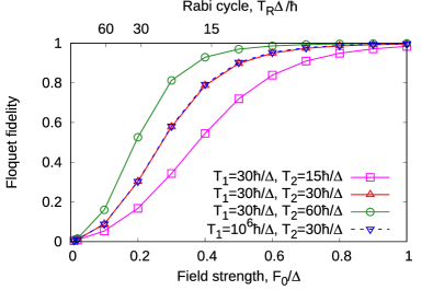
Figure 2: Floquet fidelity of nonequilibrium steady states in the resonantly driving condition, $\hbar\Omega=\Delta$. The results with different relaxation conditions are shown as functions of applied field strength $F_{0}$. The secondary $x$-axis shows the corresponding Rabi cycle, $T_{R}=2\pi/\Omega_{R}$ with the Rabi frequency $\Omega_{R}=F_{0}/\hbar$.

Next we study the quasienergy spectrum of the driven open-quantum system, computed by the stochastic trajectory approach, Eq. (24), employing a $\sin^{2}$ envelope for the probe field $f(t)$ with the total duration of $200\pi\hbar/\Delta$, which is $100$ optical cycles of the pump field in the resonant condition, $\hbar\Omega=\Delta$.

Figure 3 shows the spectral density as a function of quasienergy $E_{q}$, which is defined by the difference of the photon-energy of the probe field $\hbar\omega$ and the energy of the detector state $\epsilon$, $E_{q}=\epsilon-\hbar\omega$. Here, the relaxation times, $T_{1}$ and $T_{2}$, are set to $30\hbar/\Delta$. The results computed with different field strength $F_{0}$ are compared in Fig. 3. The result without driving field (black solid line) shows a peak at $-\Delta/2$, which is the single-particle energy of the ground state $|g\rangle$. Because the quantum jump process in the stochastic approach with the Lindblad operators, Eq. (7) and Eq. (8), does not affect the ground state, $|g\rangle$, the linewidth of the ground state spectrum is solely caused by the bandwidth of the probe pulse. When a driving field is applied, the quasienergy peak is broadened (red-dashed line) because the dissipative mechanism is activated by the photo-excitation. Once the applied field strength becomes strong enough, the quasienergy peak is split into two peaks, reflecting the well-known Rabi splitting (see green-dotted and blue-dash-dot lines). These results demonstrate that signatures of Floquet states are disturbed by dissipation, and they can be evident only when the driving field strength is strong enough to overcome the dissipation contribution.

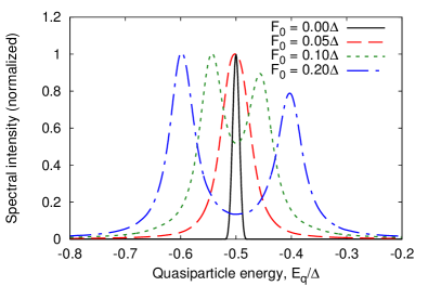
Figure 3: Quasienergy spectrum computed by Eq. (24) under resonant driving ($\hbar\Omega=\Delta$). The results for different driving field strength are shown. Here, we set both the longitudinal and transverse relaxation times to $T_{1}=T_{2}=30\hbar/\Delta$. Note the maximum value of the spectral density are normalized to one for each field strength.

Let us now take a closer look at the role of the decoherence in the formation of Floquet states. For this purpose, we compute the quasienergy spectrum while also changing the decoherence time, $T_{2}$. Figure 4 shows the computed quasienergy spectra with Eq. (24). In these calculations, the longitudinal relaxation time is fixed to $T_{1}=30\hbar/\Delta$, and the field strength is fixed to $F_{0}=0.2\Delta$. The period of the corresponding Rabi flopping is $T_{R}=2\pi/F_{0}\approx 30\hbar/\Delta$. The red-solid line in Fig. 4 shows the result with the decoherence time $T_{2}$ of $30\hbar/\Delta$, which is almost identical to the period of the Rabi oscillation $T_{R}$, but it clearly shows the double peak structure of the Rabi splitting, where the corresponding Rabi splitting energy is $\hbar\Omega_{R}=F_{0}=0.2\Delta$. The green-dashed line shows the result with $T_{2}=10\hbar/\Delta$, which is almost one third of the Rabi cycle $T_{R}$. The result clearly demonstrates that the key feature of Floquet states, namely Rabi-splitting, is still fairly visible even though the decoherence time is substantially shorter than the Rabi cycle ($T_{2}<T_{R}$). However, if the decoherence time $T_{2}$ is further halved and is set to $T_{2}=5\hbar/\Delta$, the double-peak structure disappears (blue dotted line). This fact indicates that the coherence should survive for, at least, one third of the period of the Rabi oscillation in order to fairly observe the Rabi splitting. Interestingly, by comparing the red-solid line and the blue-dotted line in Fig. 4, one can clearly see that the disappearance of the double-peak structure originates from not only the line-broadening but also the collapse of the gap. This fact further implies that the formation of the Floquet states are significantly disturbed due to loss of coherence.

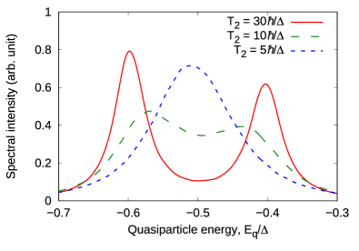
Figure 4: Quasienergy spectrum computed by Eq. (24) under resonant driving ($\hbar\Omega=\Delta$). The results for different decoherence time $T_{2}$ are shown. Here, we set the longitudinal relaxation time $T_{1}$ to $30\hbar/\Delta$, and the field strength $F_{0}$ to $0.2\Delta$.

Next, we explore the role of the dissipation in the nonequilibrium steady state based on an analysis of the microscopic energy flow. Figure 5 schematically shows the energy flow among the external driver (external field), the subsystem, and the bath. As seen from the figure, we consider two kinds of energy flow, $P_{ext}(t)$ and $P_{dis}(t)$: $P_{ext}(t)$ is the energy flow from the external field to the subsystem, and $P_{dis}(t)$ is that from the environment (dissipation) to the subsystem. The energy flow from the external field to the subsystem $P_{ext}$ can be evaluated with the Joule heating (see Appendix A for details) as

$$P_{ext}(t) = \mathrm{Tr}\left\{\frac{1}{i\hbar}\left[\frac{\Delta}{2}\sigma_{z},H(t)\right]\rho(t)\right\}$$ (29)

$$= \frac{\Delta F_{0}}{\hbar}\sin(\Omega t)\mathrm{Tr}\left\{\sigma_{y}\rho(t)\right\}.$$

Because of the total energy conservation law, the energy change of the subsystem has to be identical to the sum of the energy transfer as

$$\frac{d}{dt}E_{s}(t)=P_{ext}(t)+P_{dis}(t),$$ (30)

where $E_{s}(t)$ is the energy of the subsystem, $E_{s}(t)=\mathrm{Tr}\left\{\Delta\sigma_{z}\rho(t)\right\}/2$. Based on this fact, we redefine $P_{dis}(t)$ as

$$P_{dis}(t)\equiv\frac{d}{dt}E_{s}(t)-P_{ext}(t).$$ (31)

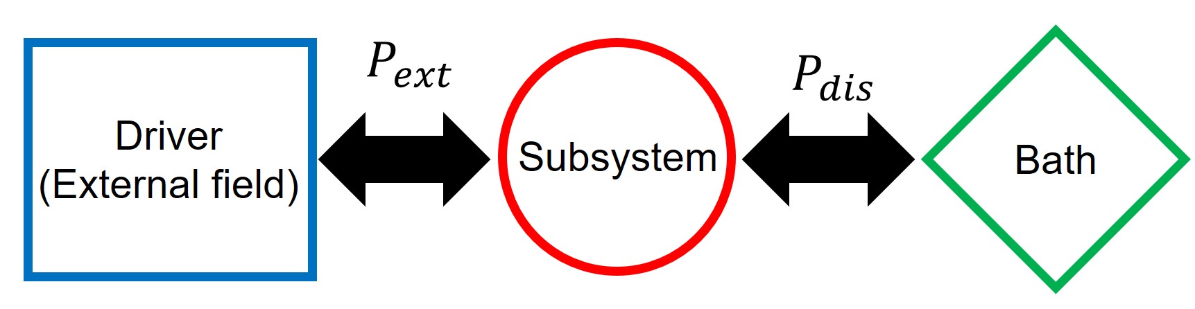
Figure 5: Schematic diagram of the energy flow among the external driver (external field), the subsystem, and the bath. Two kinds of energy flow exist: One is the flow from the external driver to the subsystem $P_{ext}$, and the other is that from the bath to the subsystem $P_{dis}$.

Figure 6 shows the energy flow in the nonequilibrium steady state as a function of time for different field strength $F_{0}$. Here, we set both the relaxation times, $T_{1}$ and $T_{2}$, to $30\hbar/\Delta$. As seen from Fig. 6 (a), the energy flow from the light to the subsystem $P_{ext}(t)$ (green-dashed line) is always positive while that from the environment to the subsystem $P_{dis}(t)$ (blue-dotted line) is always negative. Therefore, the transferred energy from the external field does not return to the external driver but it is completely dissipated by the environment in the weak field regime. Hence, the energy exchange between the subsystem and the external driver is significantly disturbed by the dissipation, and the formation of Floquet states is prevented. As shown in Fig. 6 (b), once the field strength becomes substantially strong ($F_{0}=0.5\Delta$), the energy flow $P_{ext}(t)$ shows a negative value around a certain time. The corresponding Floquet fidelity $S_{F}$ for this field strength is about $0.9$ (see Fig. 2). This fact indicates that the transferred energy from the external driver to the subsystem is not completely dissipated to the environment, but a part of the transferred energy is returned to the external driver. Thus, the energy exchange between the subsystem and the external driver becomes possible, and the corresponding Floquet states are fairly formed. As shown in Fig. 6 (c), once the field strength becomes very strong ($F_{0}=\Delta$), the energy flow $P_{ext}(t)$ becomes dominant, compared with the dissipation $P_{dis}(t)$, and almost all of the transferred energy from the external driver to the subsystem returns back to the driver. As a result, the corresponding Floquet fidelity $S_{F}$ becomes almost unity (see Fig. 2), and the Floquet states are almost perfectly realized.

To comprehensively study the role of $T_{1}$ and $T_{2}$, we further repeated the energy flow analysis with different relaxation conditions (see Appendix B for details). As a result, we found that the qualitative behavior of the energy flow does not depend on $T_{1}$ while it can be affected by $T_{2}$. This fact further indicates that the longitudinal relaxation characterized by $T_{1}$ does not disturb the energy exchange between the subsystem and the external driver, and it does not disturb the formation of Floquet states. In contrast, the decoherence characterized by $T_{2}$ can disturb the energy exchange and the formation of Floquet states.

Based on the above analysis, the energy exchange between the system and the driving field is expected to play an important role to realize Floquet state as well as the photo-dressed states. This results may further indicate a possibility to stabilize Floquet states by tuning the energy exchange with additional controlling fields such as a secondary laser field. A possibility of stabilization of Floquet states with multi-color laser fields will be investigated in future work based on these findings.

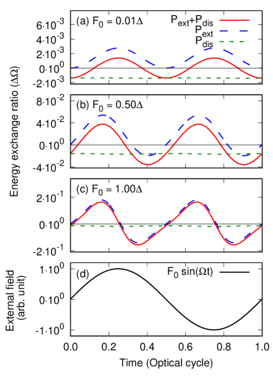
Figure 6: Energy flow in the nonequilibrium steady state among the subsystem, the external driver and the environment under resonant driving ($\hbar\Omega=\Delta$) as a function of time. The results for different field strength are shown: (a) $F_{0}=0.01\Delta$, (b) $F_{0}=0.50\Delta$, and (c) $F_{0}=1.00\Delta$.

At the end of this subsection, we investigate the nonequilibrium steady state under the significant decoherence, where the decoherence time is substantially shorter than the cycle of the external driving. Thus, the coherence does not survive even for the single period of the driving field. Under such significant decoherence, can Floquet states be still realized? To address this question, we investigate the nonequilibrium steady state by setting $T_{1}$ to $30\hbar/\Delta$ and $T_{2}$ to $T_{cycle}/2$, which is the half cycle of the external driving.

Figure 7 shows the computed Floquet fidelity as a function of the driving field strength $F_{0}$. In the weak field limit, the Floquet fidelity becomes zero, indicating that the Floquet states is significantly disturbed by the decoherence. In contrast, the Floquet fidelity asymptotically reaches to one in the strong field regime, indicating that the decoherence effect is overcome by the strong driving, and the Floquet states are stabilized. This result clearly demonstrates that Floquet states can be realized with a sufficiently strong driving field even under the influence of significant decoherence, where the coherence is lost before the single-cycle of the external driving.

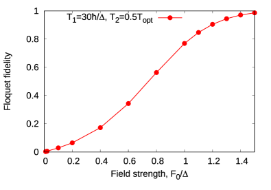
Figure 7: Floquet fidelity as a function of the field strength $F_{0}$ in the resonantly driving condition, $\hbar\Omega=\Delta$. Here, we set the driving frequency $\Omega$ to $\Delta/\hbar$, the longitudinal relaxation time $T_{1}$ to $30\hbar/\Delta$, the decoherence time $T_{2}$ to the half cycle of the driving $T_{cycle}/2$.

III.2 Off-resonance

Here, we investigate the nonequilibrium steady state in an off-resonant condition. For this purse, we set the driving frequency $\Omega$ of the field to one third of the gap of the system, $\Delta/3\hbar$. This is nothing else than the three-photon resonance condition. Note that the three-photon absorption process is the lowest order nonlinear photo-excitation in the present model because the even-photon absorption processes, including the two-photon absorption, are forbidden by the symmetry of the Hamiltonian. In this subsection, we further set both the relaxation times, $T_{1}$ and $T_{2}$, to $30\hbar/\Delta$.

Figure 8 (a) shows the computed Floquet fidelity $S_{F}$ as a function of field strength $F_{0}$. In the weak field regime, the Floquet fidelity is close to one, indicating that the Floquet states are almost perfectly realized. This behavior is qualitatively different from that in the resonant condition (see Fig. 2): in the resonant condition, the Floquet fidelity is almost zero in the weak field regime. The qualitative difference of the two conditions can be explained by the photo-induced population transfer Sato et al. (2019a, b): While the dissipation mechanism is activated in the resonant condition because the excited state is populated by the resonant excitation, it is not activated in the off-resonant condition because the population transfer cannot occur due to the energy gap. Once the field strength becomes substantially strong, the Floquet fidelity becomes small, indicating that the Floquet states are disturbed by the dissipation. Then, when the field strength becomes even stronger, the Floquet fidelity approaches to one again. To elucidate the mechanism of the temporal reduction of the Floquet fidelity in Fig. 8 (a), we evaluate Floquet quasienergies based on the Fourier decomposition of the Floquet states,

$$|\psi_{F,a}(t)\rangle=\sum_{m}e^{-i\frac{\epsilon_{a,m}}{\hbar}t}|u_{a,m}\rangle,$$ (32)

where $\epsilon_{a,m}$ is the replicated Floquet-quasienergy defined as $\epsilon_{a,m}=\epsilon_{a}+m\hbar\Omega$, and $|u_{a,m}\rangle$ is the corresponding Fourier component.

Figure 8 (b) shows the computed Floquet quasienergy $\epsilon_{a,m}$ as a function of the applied field strength, $F_{0}$. The false color shows the norm of the corresponding state, $\langle u_{a,m}|u_{a,m}\rangle$. In the weak field limit, the states have the bare gap of $\Delta$. As the field strength increases, the gap becomes larger due to the dynamical Stark effect. When the field strength $F_{0}$ is close to $\Delta$, the gap between the dominantly populated states reaches $5\Delta/3$, which is identical to five times the photon-energy of the applied field, $\hbar\Omega=\Delta/3$. Therefore, the five-photon absorption process is expected to occur around this field strength. Indeed, the Floquet quasienergy spectrum in Fig. 8 (b) clearly shows the energy splitting around this field strength. Evidently, the Floquet fidelity $S_{F}$ is sharply reduced around this five-photon absorption regime, comparing Figs. 8 (a) and (b). Therefore, the destruction of the Floquet states can be understood as the activation of the dissipative mechanism through multi-photon processes. Importantly, the three-photon absorption process, which is the lowest possible multi-photon absorption process does not have a substantial impact on the activation of the dissipation because it is significantly suppressed by the band-gap renormalization due to the dynamical Stark effect.

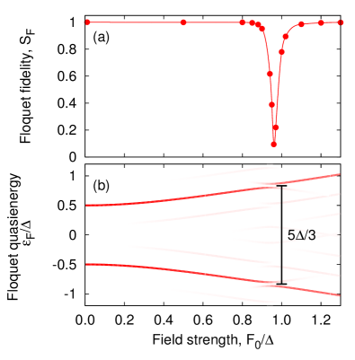
Figure 8: (a) Floquet fidelity as a function of the field strength $F_{0}$ in the off-resonant condition, $\hbar\Omega=\Delta/3$. Here, we set both the relaxation times, $T_{1}$ and $T_{2}$, to $30\hbar/\Delta$. (b) the Floquet quasienergy spectrum as a function of the field strength $F_{0}$ in the off-resonant condition.

The above finding indicates that the population transfer (heating effect) has a significant impact in the disappearance of the Floquet states even in the off-resonant condition.

IV Summary

In this work, we investigated some basic properties of nonequilibrium steady states driven by periodic driving fields under the influence of dissipation. We employed the Maxwell-Bloch equation Arecchi and Bonifacio (1965); Meier et al. (2007) and equivalent formulations in order to evaluate the Floquet fidelity $S_{F}$ and the quasienergy spectrum of the nonequilibrium steady state.

First, we investigated the properties of the nonequilibrium steady state in the resonant driving condition. In the weak field strength limit, the Floqeut fidelity approaches to zero. This fact indicates that the Floquet states are significantly destructed by the system-environment interaction that is triggered by the photoexcited population $\rho_{ee}(t)=\langle e|\rho(t)|e\rangle$. When the field strength becomes substantial, the Floquet fidelity monotonically increases and asymptotically approaches to one, reflecting that the nonequilibrium steady states are perfectly described by the Floquet states. This behavior can be understood in terms of the competition of the driving field contribution and the dissipation contribution. In the weak field regime, the driving field contribution is overcome by the dissipation contribution. As a result, the Floquet states are significantly disturbed, and the Floquet fidelity $S_{F}$ becomes small. Once the field strength becomes strong enough, the driving field contribution becomes dominant, compared with the dissipation contribution. As a result, the Floquet states are stabilized, and the Floqeut fidelity approaches to one.

To elucidate the detailed roles of the dissipation, we evaluated the Floquet fidelity by varying the relaxation times, $T_{1}$ and $T_{2}$. As a result, we found that the longitudinal relaxation time $T_{1}$ does not have a direct impact on the formation of Floquet states while the transverse relaxation time (decoherence time) $T_{2}$ has a significant impact on the formation and the destruction of Floquet states. These results indicate that the coherence plays an important role in the formation of Floquet states and it has to survive for a relevant timescale to realize Floquet states.

Then, employing the stochastic wavefunction approach, we investigate the quasienergy structure of the nonequilibrium steady state in the resonant condition. Consistently with the above Floquet fidelity analysis, the quasienergy spectrum shows the double peak structure as a signature of the Rabi-splitting once the applied field strength becomes strong enough. To elucidate the role of the decoherence in the formation of the Floquet features, we computed the energy spectrum by varying the decoherence time $T_{2}$ (see Fig. 4). As a result, we found that the decoherence destructs the feature of the Floquet states in the energy spectrum by causing the collapse of the gap of the Rabi splitting. This fact clearly demonstrates that the decoherence does not only hide the Floquet features in the spectrum due to the line-broadening but also destructs the Floquet states themselves. Therefore, the suppression of the decoherence effects is expected to be very important to optically control material functionalities via the Floquet engineering.

Next, we studied the nonequilibrium steady state under the influence of the significant decoherence in order to address the following question: Can Floquet states be formed even if the coherence is annihilated before the optical cycle? As a result of the analysis, we demonstrated that the Floquet states can indeed be formed even under the significant decoherence once the field strength becomes strong enough (see Fig. 7). This fact indicates that the period of driving fields is not a relevant timescale for the formation of Floquet states.

Finally, we investigated the Floquet fidelity in the off-resonant condition, where the photon-energy of the driving field is set to the one third of the gap, $\hbar\Omega=\Delta/3$. In the off-resonant condition, the Floquet fidelity becomes almost one in the weak field regime in contrast to the resonant condition. This result indicates that the Floquet states are well formed in the off-resonant weak field regime because the photo-excitation is forbidden by the gap and the dissipation contribution is not activated. Furthermore, we found that the Floquet fidelity can be substantially reduced once the multi-photon excitation becomes relevant because the photo-excitation further triggers the dissipation mechanism and the Floquet states are disturbed by the system-environment interaction.

The above findings clearly demonstrate that heating effects and/or photo-excitation effects can significantly affect the formation of Floquet states because the excess energy of excited systems can be dissipated to its environment through the system-environment interaction, which further destructs the coherence of the field driven dynamics. Therefore, one can expect that the Floquet states may be stabilized by reducing the effective energy dissipation to the environment with additional external driving fields. For example, one may realize the stabilized Floquet states with multi-color laser fields; one color mainly drives the Floquet states, and the other colors stabilize them by renormalizing the energy dissipation. This is also known as optical-control of coherence through the control of dissipation, and it may further introduce additional degree of freedoms in the Floquet engineering and the optical-control itself.

In this work, we employed the simplest Markovian master equation to clarify the primary role of dissipation in driven quantum systems. Therefore, a role of memory effects in driven quantum systems, especially in the context of the formation of dressed states, has not been explored yet. Although theoretical treatment of such memory effects with non-Markovian master equations is much more difficult than the simple Markovian treatment, the role of the memory effects has to be clarified towards the optical-control of material functionalities and phases of matter because rich physical properties may be realized in driven quantum systems relaying on complex memory effects. Work along these lines with non-Markovian quantum master equations is already under way.

Appendix A Energy transfer from external fields to quantum systems

Here, we revisit the energy transfer from an external field to the quantum two-level system. To purely evaluate the energy exchange between the external field and the quantum system, we disregard the dissipation and assume that the dynamical system is described by the following quantum Liouville equation

$$\frac{d}{dt}\rho(t)=\frac{\left[H(t),\rho(t)\right]}{i\hbar},$$ (33)

with the $2\times 2$ Hamiltonian matrix

$$H(t)=\frac{\Delta}{2}\sigma_{z}+F_{0}\sin(\Omega t)\sigma_{x}.$$ (34)

The energy of the quantum system is defined with the unperturbed Hamiltonian $\Delta\sigma_{z}/2$ as

$$\tilde{E}_{s}(t)=\mathrm{Tr}\left\{\frac{\Delta}{2}\sigma_{z}\rho(t)\right\}.$$ (35)

Thus the energy change of the subsystem by the external field is evaluated as

$$P_{ext}(t) \equiv \frac{d}{dt}\tilde{E}_{s}(t)$$ (36)

$$= \mathrm{Tr}\left\{\frac{1}{i\hbar}\left[\frac{\Delta}{2}\sigma_{z},H(t)\right]\rho(t)\right\}$$

$$= \frac{\Delta F_{0}}{\hbar}\sin(\Omega t)\mathrm{Tr}\left\{\sigma_{y}\rho(t)\right\}.$$

This is nothing but the energy gain of the subsystem purely from the external field, and it is introduced as $P_{ext}(t)$ in Eq. (29).

In the main text, we further define the energy flow from the environment as the difference between the total energy change $dE_{s}(t)/dt$ and the pure external-field contribution $P_{ext}(t)$ in Eq. (30).

Appendix B Energy exchange analysis with several relaxation conditions

For a comprehensive study, we repeat the energy flow analysis shown in Fig. 6 with different relaxation conditions. Note that, in the analysis of Fig. 6, the relaxation times, $T_{1}$ and $T_{2}$, are set to $30\hbar/\Delta$.

First, we investigate the effect of the longitudinal relaxation time $T_{1}$ in the energy flow. For this purpose, we set $T_{1}$ to $300\hbar/\Delta$, which is ten times larger than the original analysis in Fig. 6, while fixing $T_{2}$ to the original value, $30\hbar/\Delta$. Figure 9 shows the computed energy flow with different field strength. Comparing Fig. 9 with Fig. 6, one sees that the qualitative behavior of the energy flow in the two relaxation conditions does not change despite the significant difference of the longitudinal relaxation time, $T_{1}$. Therefore $T_{1}$ does not affect the energy exchange between the subsytem and the external driver.

Figure 9: Energy flow in the nonequilibrium steady state among the subsystem, the external driver and the environment under resonant driving ($\hbar\Omega=\Delta$) as a function of time. Here, $T_{1}$ is set to $300\hbar/\Delta$ and $T_{2}$ is set to $30\hbar/\Delta$. The results for different field strength are shown: (a) $F_{0}=0.01\Delta$, (b) $F_{0}=0.50\Delta$, and (c) $F_{0}=1.00\Delta$.

Next, we investigate the effect of the transverse relaxation time $T_{2}$ in the energy flow. For this purpose, we set $T_{2}$ to $10\hbar/\Delta$, which is three times shorter than the original analysis in Fig. 6, while fixing $T_{1}$ to the original value, $30\hbar/\Delta$. Figure 10 shows the computed energy flow with different field strength. In the weak field regime ($F_{0}=0.01\Delta$), Fig. 10 (a) and Fig. 6 (a) do not show the qualitative difference because all the transferred energy to the system is dissipated and no energy returns to the external driver. In contrast, by comparing Fig. 10 (b) and Fig. 6 (b), one can clearly see that the larger ratio of the transferred energy is dissipated in the case of the stronger decoherence ($T_{2}=10\hbar/\Delta$) compared with the weaker decoherence ($T_{2}=30\hbar/\Delta$). Therefore $T_{2}$ can directly affect the energy exchange between the subsystem and the external driver.

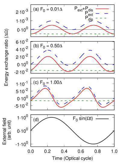
Figure 10: Energy flow in the nonequilibrium steady state among the subsystem, the external driver and the environment under resonant driving ($\hbar\Omega=\Delta$) as a function of time. Here, $T_{1}$ is set to $30\hbar/\Delta$ and $T_{2}$ is set to $10\hbar/\Delta$. The results for different field strength are shown: (a) $F_{0}=0.01\Delta$, (b) $F_{0}=0.50\Delta$, and (c) $F_{0}=1.00\Delta$.

Based on the above findings, we conclude that the longitudinal relaxation with $T_{1}$ does not affect the energy exchange between the subsystem and the external driver while the transverse relaxation with $T_{2}$ can significantly affect the energy exchange. This conclusion may be counterintuitive because the longitudinal relaxation with $T_{1}$ directly links the energy dissipation while the transverse relaxation with $T_{2}$ does not change the subsystem energy when the subsystem is undriven ($F_{0}=0$). The apparent inconsistency can be explained by the efficiency of the energy return to the external driver with coherent driving: If the subsystem keeps the perfect coherence ($T_{2}=\infty$), the subsystem shows the Rabi flopping, realizing the perfect energy exchange as all the transferred energy to the subsystem returns to the external driver. However, once the coherent dynamics is disturbed by the decoherence, the perfect Rabi flopping is destroyed and all the transferred energy cannot return to the driver anymore. In this regard, the efficiency of the energy return is affected by the decoherence. Since the subsystem is connected to the bath, the unreturned energy is simply dissipated to the bath. This scenario can explain the apparent inconsistency of the energy dissipation and the relaxation times, $T_{1}$ and $T_{2}$, further indicating the significance of the preservation of coherence in the driven dynamics to realize Floquet states.

References

- Franken et al. (1961) P. A. Franken, A. E. Hill, C. W. Peters, and G. Weinreich, Phys. Rev. Lett. 7, 118 (1961).
- Butcher and Cotter (1990) P. N. Butcher and D. Cotter, The elements of nonlinear optics, Vol. 9 (Cambridge university press, 1990).
- Boyd (2008) R. W. Boyd, Nonlinear Optics (Academic Press, New York, 2008).
- Mourou et al. (2012) G. Mourou, N. Fisch, V. Malkin, Z. Toroker, E. Khazanov, A. Sergeev, T. Tajima, and B. L. Garrec, Optics Communications 285, 720 (2012).
- Flick et al. (2017) J. Flick, M. Ruggenthaler, H. Appel, and A. Rubio, Proceedings of the National Academy of Sciences 114, 3026 (2017).
- Ruggenthaler et al. (2018) M. Ruggenthaler, N. Tancogne-Dejean, J. Flick, H. Appel, and A. Rubio, Nature Reviews Chemistry 2, 0118 (2018).
- Krausz and Ivanov (2009) F. Krausz and M. Ivanov, Rev. Mod. Phys. 81, 163 (2009).
- Krausz and Stockman (2014) F. Krausz and M. I. Stockman, Nature Photonics 8, 205 (2014).
- Basov et al. (2017) D. N. Basov, R. D. Averitt, and D. Hsieh, Nature Materials 16, 1077 (2017).
- Schiffrin et al. (2012) A. Schiffrin, T. Paasch-Colberg, N. Karpowicz, V. Apalkov, D. Gerster, S. Mühlbrandt, M. Korbman, J. Reichert, M. Schultze, S. Holzner, J. V. Barth, R. Kienberger, R. Ernstorfer, V. S. Yakovlev, M. I. Stockman, and F. Krausz, Nature 493, 70 (2012).
- Schultze et al. (2012) M. Schultze, E. M. Bothschafter, A. Sommer, S. Holzner, W. Schweinberger, M. Fiess, M. Hofstetter, R. Kienberger, V. Apalkov, V. S. Yakovlev, M. I. Stockman, and F. Krausz, Nature 493, 75 (2012).
- Schultze et al. (2014) M. Schultze, K. Ramasesha, C. Pemmaraju, S. Sato, D. Whitmore, A. Gandman, J. S. Prell, L. J. Borja, D. Prendergast, K. Yabana, D. M. Neumark, and S. R. Leone, Science 346, 1348 (2014).
- Lucchini et al. (2016) M. Lucchini, S. A. Sato, A. Ludwig, J. Herrmann, M. Volkov, L. Kasmi, Y. Shinohara, K. Yabana, L. Gallmann, and U. Keller, Science 353, 916 (2016).
- Mashiko et al. (2016) H. Mashiko, K. Oguri, T. Yamaguchi, A. Suda, and H. Gotoh, Nature Physics 12, 741 (2016).
- Schlaepfer et al. (2018) F. Schlaepfer, M. Lucchini, S. A. Sato, M. Volkov, L. Kasmi, N. Hartmann, A. Rubio, L. Gallmann, and U. Keller, Nature Physics 14, 560 (2018).
- Siegrist et al. (2019) F. Siegrist, J. A. Gessner, M. Ossiander, C. Denker, Y.-P. Chang, M. C. Schröder, A. Guggenmos, Y. Cui, J. Walowski, U. Martens, J. K. Dewhurst, U. Kleineberg, M. Münzenberg, S. Sharma, and M. Schultze, Nature 571, 240 (2019).
- Volkov et al. (2019) M. Volkov, S. A. Sato, F. Schlaepfer, L. Kasmi, N. Hartmann, M. Lucchini, L. Gallmann, A. Rubio, and U. Keller, Nature Physics 15, 1145 (2019).
- Fausti et al. (2011) D. Fausti, R. I. Tobey, N. Dean, S. Kaiser, A. Dienst, M. C. Hoffmann, S. Pyon, T. Takayama, H. Takagi, and A. Cavalleri, Science 331, 189 (2011).
- Mitrano et al. (2016) M. Mitrano, A. Cantaluppi, D. Nicoletti, S. Kaiser, A. Perucchi, S. Lupi, P. Di Pietro, D. Pontiroli, M. Riccò, S. R. Clark, D. Jaksch, and A. Cavalleri, Nature 530, 461 (2016).
- Sommer et al. (2016) A. Sommer, E. M. Bothschafter, S. A. Sato, C. Jakubeit, T. Latka, O. Razskazovskaya, H. Fattahi, M. Jobst, W. Schweinberger, V. Shirvanyan, V. S. Yakovlev, R. Kienberger, K. Yabana, N. Karpowicz, M. Schultze, and F. Krausz, Nature 534, 86 (2016).
- Oka and Aoki (2009) T. Oka and H. Aoki, Phys. Rev. B 79, 081406 (2009).
- Dunlap and Kenkre (1986) D. H. Dunlap and V. M. Kenkre, Phys. Rev. B 34, 3625 (1986).
- Großmann and Hänggi (1992) F. Großmann and P. Hänggi, EPL 18, 571 (1992).
- Eckardt (2017) A. Eckardt, Rev. Mod. Phys. 89, 011004 (2017).
- Shin et al. (2018) D. Shin, H. Hübener, U. De Giovannini, H. Jin, A. Rubio, and N. Park, Nature Communications 9, 638 (2018).
- Giovannini and Hübener (2019) U. D. Giovannini and H. Hübener, Journal of Physics: Materials 3, 012001 (2019).
- Claassen et al. (2019) M. Claassen, D. M. Kennes, M. Zingl, M. A. Sentef, and A. Rubio, Nature Physics 15, 766 (2019).
- Kohler et al. (1997) S. Kohler, T. Dittrich, and P. Hänggi, Phys. Rev. E 55, 300 (1997).
- Grifoni and Hänggi (1998) M. Grifoni and P. Hänggi, Physics Reports 304, 229 (1998).
- Restrepo et al. (2016) S. Restrepo, J. Cerrillo, V. M. Bastidas, D. G. Angelakis, and T. Brandes, Phys. Rev. Lett. 117, 250401 (2016).
- Hartmann et al. (2017) M. Hartmann, D. Poletti, M. Ivanchenko, S. Denisov, and P. Hänggi, New Journal of Physics 19, 083011 (2017).
- Kohn (2001) W. Kohn, Journal of Statistical Physics 103, 417 (2001).
- Shirai et al. (2015) T. Shirai, T. Mori, and S. Miyashita, Phys. Rev. E 91, 030101 (2015).
- Shirai et al. (2016) T. Shirai, J. Thingna, T. Mori, S. Denisov, P. Hänggi, and S. Miyashita, New Journal of Physics 18, 053008 (2016).
- Engelhardt et al. (2019) G. Engelhardt, G. Platero, and J. Cao, Phys. Rev. Lett. 123, 120602 (2019).
- Magazzù et al. (2017) L. Magazzù, S. Denisov, and P. Hänggi, Phys. Rev. A 96, 042103 (2017).
- Magazzù et al. (2018) L. Magazzù, S. Denisov, and P. Hänggi, Phys. Rev. E 98, 022111 (2018).
- Dehghani et al. (2014) H. Dehghani, T. Oka, and A. Mitra, Phys. Rev. B 90, 195429 (2014).
- Dehghani et al. (2015) H. Dehghani, T. Oka, and A. Mitra, Phys. Rev. B 91, 155422 (2015).
- Wilson et al. (2007) C. M. Wilson, T. Duty, F. Persson, M. Sandberg, G. Johansson, and P. Delsing, Phys. Rev. Lett. 98, 257003 (2007).
- Deng et al. (2015) C. Deng, J.-L. Orgiazzi, F. Shen, S. Ashhab, and A. Lupascu, Phys. Rev. Lett. 115, 133601 (2015).
- Magazzù et al. (2018) L. Magazzù, P. Forn-Díaz, R. Belyansky, J.-L. Orgiazzi, M. A. Yurtalan, M. R. Otto, A. Lupascu, C. M. Wilson, and M. Grifoni, Nature Communications 9, 1403 (2018).
- Wang et al. (2013) Y. H. Wang, H. Steinberg, P. Jarillo-Herrero, and N. Gedik, Science 342, 453 (2013).
- McIver et al. (2019) J. W. McIver, B. Schulte, F.-U. Stein, T. Matsuyama, G. Jotzu, G. Meier, and A. Cavalleri, Nature Physics (2019), 10.1038/s41567-019-0698-y.
- Sato et al. (2019a) S. A. Sato, J. W. McIver, M. Nuske, P. Tang, G. Jotzu, B. Schulte, H. Hübener, U. De Giovannini, L. Mathey, M. A. Sentef, A. Cavalleri, and A. Rubio, Phys. Rev. B 99, 214302 (2019a).
- Sato et al. (2019b) S. A. Sato, P. Tang, M. A. Sentef, U. D. Giovannini, H. Hübener, and A. Rubio, New Journal of Physics 21, 093005 (2019b).
- Hübener et al. (2017) H. Hübener, M. A. Sentef, U. de Giovannini, A. F. Kemper, and A. Rubio, Nature Communications 8, 13940 (2017).
- Hone et al. (2009) D. W. Hone, R. Ketzmerick, and W. Kohn, Phys. Rev. E 79, 051129 (2009).
- Seetharam et al. (2015) K. I. Seetharam, C.-E. Bardyn, N. H. Lindner, M. S. Rudner, and G. Refael, Phys. Rev. X 5, 041050 (2015).
- Arecchi and Bonifacio (1965) F. Arecchi and R. Bonifacio, IEEE Journal of Quantum Electronics 1, 169 (1965).
- Meier et al. (2007) T. Meier, P. Thomas, and S. W. Koch, Coherent semiconductor optics: from basic concepts to nanostructure applications (Springer Science & Business Media, 2007).
- Meier et al. (1994) T. Meier, G. von Plessen, P. Thomas, and S. W. Koch, Phys. Rev. Lett. 73, 902 (1994).
- Moulet et al. (2017) A. Moulet, J. B. Bertrand, T. Klostermann, A. Guggenmos, N. Karpowicz, and E. Goulielmakis, Science 357, 1134 (2017).
- Luu et al. (2015) T. T. Luu, M. Garg, S. Y. Kruchinin, A. Moulet, M. T. Hassan, and E. Goulielmakis, Nature 521, 498 (2015).
- Yoshikawa et al. (2017) N. Yoshikawa, T. Tamaya, and K. Tanaka, Science 356, 736 (2017).
- Breuer et al. (2002) H.-P. Breuer, F. Petruccione, et al., The theory of open quantum systems (Oxford University Press, Oxford, 2002).
- Lidar (2019) D. A. Lidar, arXiv:1902.00967 [quant-ph] (2019).
- Cardona and Ley (1978) M. Cardona and L. Ley, Photoemission in Solids I (Springer, Berlin, 1978).
- Damascelli et al. (2003) A. Damascelli, Z. Hussain, and Z.-X. Shen, Rev. Mod. Phys. 75, 473 (2003).
- Löwdin (1955) P.-O. Löwdin, Phys. Rev. 97, 1474 (1955).