Spontaneous velocity alignment in Motility-induced Phase Separation

Abstract

We study a system of purely repulsive spherical self-propelled particles in the minimal set-up inducing Motility-Induced Phase Separation (MIPS). We show that, even if explicit alignment interactions are absent, a growing order in the velocities of the clustered particles accompanies MIPS. Particles arrange into aligned or vortex-like domains. Their sizes increase as the persistence of the self-propulsion grows, an effect that is quantified studying the spatial correlation function of the velocities. We explain the velocity-alignment by unveiling a hidden alignment interaction of the Vicsek-like form, induced by the interplay between steric interactions and self-propulsion. As a consequence, we argue that the MIPS transition cannot be fully understood in terms of a scalar field, the density, since the collective orientation of the velocities should be included in effective coarse-grained descriptions.

Fishes Ward et al. (2008), birds Ballerini et al. (2008) or insects Attanasi et al. (2014) often display fashinating collective behaviors such as flocking Ballerini et al. (2008); Mora et al. (2016) and swarming Cavagna et al. (2017), where all units of a group move coherently producing intriguing dynamical patterns. A different mode of organization of living organisms is clustering, for instance in bacterial colonies Dell’Arciprete et al. (2018), such as E. Coli Berg (2008), Myxococcus xanthus Peruani et al. (2012) or Thiovulum majus Petroff et al. (2015), relevant for histological cultures in several areas of medical and pharmaceutical sciences. Out of the biological realm, the occurrence of stable clusters Bialké et al. (2015a); Palacci et al. (2013); Buttinoni et al. (2013); Ginot et al. (2018), stable chains Yan et al. (2016) or vortices Bricard et al. (2015) in activated colloidal particles, e.g. autophoretic colloids or Janus disks Howse et al. (2007); Takatori et al. (2016), offers an interesting challenge for the design of new materials.

Even if the microscopic details differ case by case, a few classes of minimal models with common coarse-grained features have been introduced in statistical physics. Units in these models are called “active” or “self-propelled” particles Marchetti et al. (2013); Ramaswamy (2010); Bechinger et al. (2016) to differentiate them from Brownian colloids which passively obey the forces of the surrounding environment. Propelling forces may be either of mechanical origin (flagella or body deformation), or of thermodynamic nature (diffusiophoresis and self-electrophoresis) Palacci et al. (2010); Theurkauff et al. (2012). In some simple and effective examples, self-propulsion is modeled as a constant force with stochastic orientation, as in the case of Active Brownian Particles (ABP) ten Hagen et al. (2011); Romanczuk et al. (2012). Thermal fluctuations play only a marginal role and stochasticity is usually due to the unsteady nature of the swimming force itself.

It is well-known that dumbells, rods and, in general, elongated microswimmers display a marked orientational order even in the absence of alignment interactions Peruani et al. (2006); Aranson and Tsimring (2003); Ginelli et al. (2010); Deseigne et al. (2010). Instead, in the literature, it is believed that explicit aligning velocity-interactions are crucial to observe velocity alignment between spherical self-propelled units Vicsek and Zafeiris (2012). This kind of interaction, such as that in the seminal Vicsek model Vicsek et al. (1995), consists in a short-range force that aligns the velocity of a target particle to the average of the neighboring ones. Vicsek interactions lead to long-range polar order Toner and Tu (1995); Toner (2012); Mahault et al. (2018), density inhomogeneities in the form of traveling bands Grégoire and Chaté (2004); Solon et al. (2015a) or periodic density waves Caussin et al. (2014). Recently, models with orientation-velocity couplings have been implemented to obtain a global polar order without assuming any explicit velocity-alignment between neighboring particles Lam et al. (2015); Giavazzi et al. (2018). Instead, the interplay between steric interactions and self-propulsions is recognized to be the minimal requirement for phase-separation in self-propelled systems. This occurs even in the absence of any attractive force Gonnella et al. (2015), at variance with passive Brownian particles. Such a phenomenon, known as Motility-induced Phase Separation (MIPS) has been largely investigated Cates and Tailleur (2015), starting from the pioneering work of Fily and Marchetti Fily and Marchetti (2012). The coexistence of clustering and velocity ordering has been recently considered, and, even if its role in MIPS is still an open question Sese-Sansa et al. (2018); Barré et al. (2015); van der Linden et al. (2019); Shi and Chaté (2018), it has been shown that may induce freezing in dense regimes Geyer et al. (2019). The alignment, characterizing Vicsek-like models Chaté et al. (2008), and the ABP phase-separation are phenomena which are usually thought to be generated by two distinct types of interactions between particles.

In the present study, we challenge the widespread idea that explicit alignment interactions are necessary to observe a growing orientational order or - equivalently - that the velocity alignment observed in Vicsek-like models do not appear in purely repulsive, spherical ABP particles. To the best of our knowledge, previous studies aimed to measure the polarization, i.e. the existence of a common orientation of the self-propelling force, but overlooked the possibility of ordering in the real particles’ velocity, that is the crucial observation of the present report.

We consider a suspension of $N$ interacting self-propelled particles, for simplicity (and without loss of generality) in two dimensions. The evolution of the center of mass coordinate of each microswimmer, $\mathbf{x}_{i}$, is described by an over-damped equation of motion with self-propulsion embodied by a time-dependent external force with constant modulus, $v_{0}$, and orientation vector, $\mathbf{n}_{i}$, of components $(\cos{\theta_{i}},\sin{\theta_{i}})$. According to the ABP scheme, the orientational angles, $\theta_{i}$, evolve as independent Wiener processes. Interactions are purely repulsive and no explicit aligning forces are included. Therefore the dynamics reads:

$$\gamma\dot{\mathbf{x}}_{i} =\mathbf{F}_{i}+\gamma v_{0}\mathbf{n}_{i}$$ (1a)

$$\dot{\theta}_{i} =\sqrt{2D_{r}}\xi_{i}\,,$$ (1b)

being $D_{r}$ the rotational diffusivity (thermal diffusion is usually negligible) while $\gamma$ is the constant drag coefficient. Steric interactions are modeled by the force $\mathbf{F}_{i}=-\nabla_{i}U_{tot}$, being $U_{tot}=\sum_{i<j}U(|{\mathbf{r}}_{ij}|)$ with ${\mathbf{r}}_{ij}=\mathbf{x}_{i}-\mathbf{x}_{j}$. We choose $U(r)$, with as a purely repulsive potential of the WCA type, namely $U(r)=4\epsilon\left[\left(\frac{\sigma}{r}\right)^{12}-\left(\frac{\sigma}{r}\right)^{6}\right]+\epsilon$, for $r\leq 2^{1/6}\sigma$ and zero otherwise. The constant $\sigma$ represents the nominal particle diameter while $\epsilon$ is the energy scale due to interactions.

Numerical integration of Eq. (1a) is performed for a system of $N$ particles in a square box of length $L$, with periodic boundary conditions. We set a packing fraction $\phi=0.64$, where MIPS is known to occur at small enough values of $D_{r}$ Fily and Marchetti (2012). Indeed, Fig. 1(a) shows the coexistence of a stable dense cluster and a dilute disordered phase, at $D_{r}=0.2$. The boundary of the cluster is highly dynamical: continuously in time, particles join the cluster and leave it, in such a way that the average cluster population does not change. In Fig. 1 (b-d) we enlarge three representative regions of the system. The bulk displays a highly ordered close-packing configuration Redner et al. (2013). The study of the pair correlation function, $g(r)$, shown in the Supplemental Materials (SM), reveals that the main peak occurs at a distance $\bar{r}<\sigma$ in the cluster: particles attain a steady-state configuration with large potential energy, where each microswimmer climbs on the repulsive potential exerted by the surrounding ones. Besides, the occurrence of a second double-split peak reveals a hexagonal lattice structure, in agreement with the direct observation and previous studies Redner et al. (2013). The colors in Figs. 1(a-d) encode the orientation, $\mathbf{n}$, of the self-propelling force which appears to lack any kind of alignment.

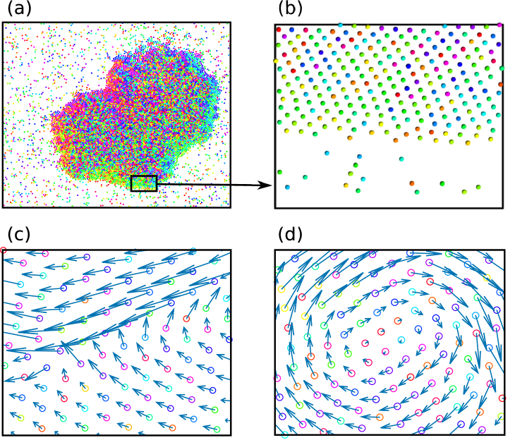
Figure 1: In panel (a) we plot a snapshot configuration, displaying MIPS, enlarging a window near the surface of the cluster. Colors encode the self-propulsion direction. Panel (c) and (d) are windows of the bulk where we plot the velocities of each particle with blue arrows, showing aligned and vortex domains, respectively. Data are obtained by simulation with $v_{0}=50$, $D_{r}=0.2$ and the other parameters as described in the text.

In Fig. 1 (c-d) we give evidence of the main novel phenomenon reported here. We draw with blue arrows the velocities, $\dot{\mathbf{x}}_{i}$, of each microswimmer which is in general different from the orientation of the active force, i.e. $\dot{\mathbf{x}}_{i}\neq\mathbf{n}_{i}v_{0}$. Despite the absence of any alignment interaction, the velocities of the microswimmers in the bulk of the cluster align, self-organizing in large oriented domains inside the cluster. Even if each $\mathbf{n}_{i}$ points randomly, particles in large groups move in the same direction (Fig. 1 c)). Such domains dynamically self-arrange continuously in time and, in some cases, evolve into vortex structures as evidenced in Fig. 1 d). The average velocity of each domain is quite smaller than $v_{0}$ (the typical speed in the absence of interactions). Further details about the velocity distributions in the different phases are contained in the SM.

The global alignment of the particles or polarization is commonly measured by considering the propulsion orientation, ${\mathbf{n}}_{i}$, of each particle, while here we focus on the velocity $\dot{\mathbf{x}}_{i}$. A possible order parameter is represented by the sum $\left|\sum_{k=1}^{N}e^{i\psi_{k}(t)}\right|$, where $\psi_{k}$ is the angle formed by the particle velocity with respect to the $x$ axis. Such a parameter has the property of being zero for particles without any alignment while it returns one for perfectly aligned particles. Unfortunately, even if restricted to particles inside a cluster, such a quantity does not reveal a clear polarization of the system because of the presence of several domains with different orientations. Thus, we introduce the spatial correlation function of the velocity orientation, $Q_{i}(r)$. We define the angular distance between two angles $d_{ij}=\min[|\psi_{i}-\psi_{j}|,2\pi-|\psi_{i}-\psi_{j}|]$, and measure the velocity alignment between particle $i$ and the neighboring particles in the circular crown of mean radius $r=k\bar{r}$, with integer $k>0$, and thickness $\bar{r}$, in such a way that

$$Q_{i}(r)=1-2\sum_{j}\frac{d_{ij}}{\mathcal{N}_{k}\pi}\,,$$ (2)

where the sum runs only over the particles in the circular shell selected by $k$ and $\mathcal{N}_{k}$ is the number of particles in that shell. Then, we define $Q(r)=\sum_{i}Q_{i}(r)/N$, which reads 1 for perfectly aligned particles in the $k$-th shell, $-1$ for anti-aligned particles and $0$ in the absence of any form of alignment. $Q(r)$ can quantify partial alignment even in the absence of global polarization. Panel (b) of Fig. 2 shows $Q(r)$ for different values of $D_{r}$ in a set of simulations with $v_{0}=50$ (the other parameters are fixed in the same way as before). In general $Q$ is a decreasing function of $r$. At large $D_{r}$ where MIPS does not occur, the alignment measured by $Q(r)$ is absent or very weak, affecting no more than the first two shells. In the MIPS configuration, the degree of alignment increases and spans larger and larger distances, when $D_{r}$ is reduced. Three snapshots with color-encoded velocity orientation are shown in panels (c-e) of Fig. 2, showing the growth of velocity-aligned domains in the cluster phase. In fig. 2(a) we investigate the nature of this ordering phenomenon by measuring the following order parameter

$$R=\int Q(r)dr\,.$$ (3)

The integral is performed over the whole cluster domain while in the absence of phase separation we consider the whole box.

To evaluate the relationship between this growing spatial velocity order and MIPS, we compare $R$ with an established order parameter for phase separation. Local packing fractions show a unimodal distribution when the system is not phase-separated and a bimodal one when phase separation occurs. The height of the peaks in the distribution identifies the most probable values of the packing fraction in the unimodal case, it corresponds to the homogeneous phase $\phi_{g}\approx\phi$. Instead, in the bimodal case, the cluster phase is identified by the peak with $\phi_{c}>\phi$ while the disordered phase by that with $\phi_{g}<\phi$. These results are reproduced as a function of $1/D_{r}$ in Fig. 2(a). At $1/D_{r}\sim 0.3$ phase separation is revealed by the transition from the single peak to the double peak in the distribution of the packing fraction. In our configuration, $\phi_{g}$ in the homogeneous phase follows continuously the values outside the cluster, which forms at a much higher packing fraction. The comparison with the curve for $R$ reveals the most interesting information of our study, that is the coincidence between the MIPS transition and the growing of the velocity-order. Indeed, $R$ reveals a two-steps behavior, being almost-zero before $1/D_{r}\sim 0.3$ and revealing a sharp, monotonic increase starting from this point.

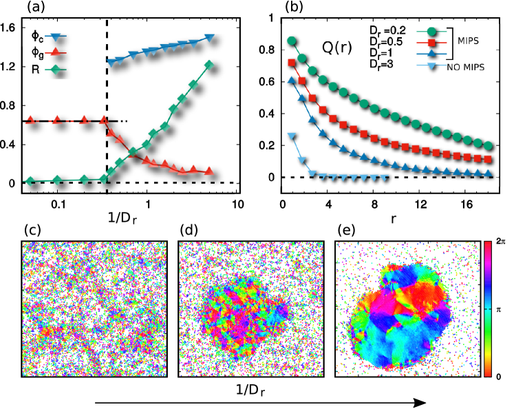
Figure 2: Panel (a): density, $\phi_{g}$ (red upper triangles) and $\phi_{c}$ (blue lower triangles) for the dilute and the cluster phase, respectively, as a function of $1/D_{r}$. Velocity-alignment order parameter, $R$ (green diamonds), as a function of $1/D_{r}$. For presentation reasons, $R$ is rescaled by a factor 6. Black dashed lines are eye-guides: the vertical one identifies the value of $1/D_{r}$ at which the MIPS-transition occurs. Instead, the horizontal lines refer to the nominal density ($\sim 0.64$) and the value of $R$ in absence of velocity alignment ($\sim 0$). Panel (b): $Q(r)$ for different values of $D_{r}$, as shown in the legend, where we specify the presence or not of the phase separation. Panel (c), (d) and (e): Snapshot configurations for three different values of $1/D_{r}$. Panel (c) is obtained for $D_{r}=3$, panel (d) for $D_{r}=1$ and panel (e) for $D_{r}=0.2$. Colors are associated with the direction of the velocity of each particle. All the simulations are realized with numerical density $\sim 0.64$, $v_{0}=50$ and the other parameters specified in the text.

To shed light on the above phenomenology we perform an exact mapping of the original ABP dynamics, Eqs. (1), in the same spirit of the Ornstein-Uhlenbeck (AOUP) model Fodor et al. (2016); Caprini et al. (2018, 2019a). In particular, we obtain an equation of motion for the microswimmer velocity, $\mathbf{v}_{i}=\dot{\mathbf{x}}_{i}$, which is an unprecedented result for ABP. In two dimensions, $\mathbf{v}_{i}$ follows:

$$\mu\dot{\mathbf{v}}_{i}=-\gamma\sum_{j=1}^{N}{\Gamma}_{ij}({\mathbf{r}}_{ij})\mathbf{v}_{j}+\mathbf{F}_{i}+\sqrt{2\gamma(\mu v_{0}^{2})}\boldsymbol{\xi}_{i}\times{\mathbf{n}}_{i}\,,$$ (4)

where $\boldsymbol{\xi}_{i}$ is the stochastic vector with components $(0,0,\xi_{i})$ and both $\mathbf{v}_{i}$ and $\mathbf{x}_{i}$ belong to the plane $xy$. The effective mass is $\mu=\gamma/D_{r}$ and the viscosity matrix $\Gamma_{ij}$ has the following structure:

$$\Gamma_{ij}^{\alpha\beta}({\mathbf{r}}_{ij})=\delta_{ij}\delta_{\alpha\beta}+\frac{1}{D_{r}\gamma}\nabla_{i\alpha}\nabla_{j\beta}\sum_{k<l}U(|{\mathbf{r}}_{kl}|)\,,$$ (5)

where Latin and Greek indices refer to the particle number and the spatial vector components, respectively. The derivation of Eq. (4) is reported in the SM. Eq. (4) is the equation of motion of an underdamped particle under the action of a space-dependent Stokes force and a multiplicative noise both in the velocity and in the position of the target microswimmer. The noise term always acts perpendicularly to $\mathbf{n}_{i}$, because of the cross product. The most interesting information contained in Eq. (4) is the fact that the dynamics of the $i$-th particle is strongly influenced not only by the positions but also by the velocities of the surrounding particles, through the matrix $\Gamma_{ij}$ which - because of the factor $1/D_{r}$ - is dominated by the velocity coupling terms. We recall that Eq. (4) is almost identical to the equation of motion of interacting AOUP particles Marconi et al. (2016), the only difference being the noise term, which in AOUP is additive and uncorrelated, i.e. $\boldsymbol{\xi}_{i}\times{\mathbf{n}}_{i}$ is replaced by a noise vector with independent components.

Inside a cluster Eq. (4) can be further simplified, taking advantage of the hexagonal spatial order: we may assume that a particle in the bulk of the cluster has $6$ neighbors at relative positions $\bar{\mathbf{r}}_{ij}$ with $j=1..6$, with constant modulus $\bar{r}=|\bar{\mathbf{r}}_{ij}|<\sigma$, as revealed, for instance, by the $g(r)$. With these assumptions, one gets for the particle at the center of the hexagon

$$\mu\dot{\mathbf{v}}=-\frac{1}{D_{r}}\sum^{6}_{j=1}\hat{H}_{j}\cdot(\mathbf{v}-\mathbf{v}_{j})-\gamma\mathbf{v}+\sqrt{2\gamma(\mu v_{0}^{2})}\boldsymbol{\xi}\times{\mathbf{n}}\,,$$ (6)

where $\hat{H}_{j}$ is the matrix coupling the central particle to the $j$-th particle and its elements depend on $\bar{r}$ and on the angle formed by $\mathbf{x}_{ij}=\mathbf{x}_{j}-\mathbf{x}_{i}$ and the $x$-axis. The matrix elements of $\hat{H}_{j}$ are reported in the SM. Equation (6) can be rewritten in terms of the average velocity vector of the $6$ neighbors $\mathbf{v}^{*}=\sum_{j=1}^{6}\mathbf{v}_{j}/6$ and takes the form

$$\mu\dot{\mathbf{v}}=-\frac{\hat{J}}{D_{r}}\cdot(\mathbf{v}-\mathbf{v}^{*})+\frac{1}{D_{r}}\sum^{6}_{j=1}\hat{H}_{j}\cdot(\mathbf{v}_{j}-\mathbf{v}^{*})-\gamma\mathbf{v}+\mathbf{k}\,,$$ (7)

with $\hat{J}=\sum_{j}^{6}\hat{H}_{j}=3\left[U^{\prime\prime}(\bar{r})+\frac{U^{\prime}(\bar{r})}{|\bar{r}|}\right]\mathcal{I}$, being $\mathcal{I}$ the identity matrix and $\mathbf{k}$ the noise vector of Eq. (6). Eqs. (6) and (7) are derived in the SM. We notice that $\left(U^{\prime\prime}(\bar{r})+\frac{U^{\prime}(\bar{r})}{|\bar{r}|}\right)>0$ which means that the first term in the rhs of Eq. (7) is a Vicsek-like force aligning the velocity of the central particle towards the average velocity vector $\mathbf{v}^{*}$ Grégoire and Chaté (2004). In two special cases the second force in the rhs of Eq. (7) vanishes: i) trivially when the $6$ neighbors have identical velocities ${\mathbf{v}}_{j}={\mathbf{v}}^{*}$; ii) when the $6$ neighbors have velocities arranged according to a vortex-like pattern. This statement is proved in the SM. In both cases at large $1/D_{r}$ the dynamics of $\mu\dot{\mathbf{v}}$ is dominated by the Vicsek-like aligning force (first term in the rhs of Eq. (7)) and one has a rapid convergence ${\mathbf{v}}\to{\mathbf{v}}^{*}$. At the end of this convergence, i.e. when the velocity of the central particle is exactly aligned with the $6$ neighbors, the aligning force disappears and the sub-dominant bath-like terms $-\gamma\mathbf{v}+\sqrt{2\gamma(\mu v_{0}^{2})}\boldsymbol{\xi}\times{\mathbf{n}}$ perturb the velocity. At this stage, the Vicsek-like force comes back into play and restores the alignment. For more general cases (i.e. when the $6$ neighbors are not aligned or are arranged in a vortex pattern), a second force, depending on the deviations $\mathbf{v}_{j}-\mathbf{v}^{*}$ with a large pre-factor $1/D_{r}$, comes into play. However, when particles are close to alignment, the terms $\mathbf{v}_{j}-\mathbf{v}^{*}$ are small and uncorrelated, so that their sum is even smaller and does not alter significantly the aligning term, as numerically checked. A rigorous general estimate of the fate of Eq. (7) is difficult.

Our analytical description in terms of effective velocities could be adapted to describe the emergent polar order of rod-like Ginelli et al. (2010); Yang et al. (2010); Bär et al. (2019) or dumbell Suma et al. (2014); Cugliandolo et al. (2017) particles, introducing the angular velocity induced by the self-propulsion.

To derive the exponential-like form of the spatial velocities correlations, we assume all particles sitting on an infinite hexagonal lattice, with each particle’s velocity connected to its $6$ neighbors by Eq. (6). Since ${\mathbf{n}}$ and ${\mathbf{v}}$ are roughly uncorrelated in the bulk, we replace the multiplicative noise with an additive uncorrelated noise, as in the AOUP case Caprini et al. (2019b). The evolution of this velocity field can be mapped, by Fourier transforming, onto a Langevin equation for each mode in the reciprocal lattice. Its steady-state solution gives the velocity structure factor or, equivalently, the spatial correlations of the velocity field. This analysis demonstrates that the correlation length of the velocity field reads

$$\lambda_{s}\approx\bar{r}\left[\frac{3}{4\gamma D_{r}}\left(U^{\prime\prime}(\bar{r})+\frac{U^{\prime}(\bar{r})}{|\bar{r}|}\right)\right]^{1/2}\,,$$ (8)

whose derivation is reported in the SM. This argument suggests a correlation length growing with $1/D_{r}$ in qualitative agreement with Fig. 2 a) and b). We suspect that terms at small wavelengths can be important, for instance, in the explanation of the vortex structures.

Our study demonstrates an unprecedented strong connection between velocity ordering and MIPS transitions. In the absence of any microscopic force that explicitly aligns velocities, we observe the emergence of velocity patterns, aligned or vortex-like domains in a dense cluster, which become more and more pronounced as the persistence of the active force increases.

We stress here the deep non-equilibrium nature revealed by our study. Such a velocity order cannot be observed in any passive Brownian suspensions of spherical particles, since, in those cases, particles’ velocities are distributed according to independent Boltzmann distributions. Thus, the growth of order in the velocity field cannot be explained in equilibrium-like theories unless an effective aligning force is introduced in a macroscopic “Hamiltonian” which is absent in the microscopic model. This would be in line with previous equilibrium-like approaches where effective attractive interactions were introduced to explain phase separation Farage et al. (2015); Rein and Speck (2016) also at the level of an effective free-energy functional Tailleur and Cates (2008); Cates and Tailleur (2013); Speck (2016); Solon et al. (2018a) or employing an effective Cahn-Hilliard equation Stenhammar et al. (2013); Speck et al. (2014). All such strategies were already challenged by observations about pressure Solon et al. (2015b, c), negative interfacial tension between the coexisting phases Bialké et al. (2015b); Patch et al. (2018) and different temperatures inside and outside the cluster Mandal et al. (2019), all inconsistent with any equilibrium-like scenario. The phenomenology discussed here represents an additional argument in favor of a purely non-equilibrium approach.

In virtue of our results, we argue that the full comprehension of MIPS cannot be obtained in terms of the density field only, but requires, at least, the employment of another vector field to account for the velocity alignment. The introduction of a vectorial field to model the velocity alignment, for instance in the framework of field theories Stenhammar et al. (2014); Wittkowski et al. (2014); Tjhung et al. (2018); Großmann et al. (2019); Solon et al. (2018b); Paoluzzi et al. (2019), may offer a new interesting perspective to increase the understanding of MIPS combined with the alignment phenomenology presented in this manuscript.

Supplemental Material of “Spontaneous velocity alignment in Motility-induced Phase Separation”

In this Supplemental Materials, we provide more details about the main phenomenology and the derivations of the analytical results reported in the main text In Sec. I, we show the pair correlations and the distribution function of the velocity modulus inside and outside the cluster. Sections II and III are devoted to the detailed derivations of Eq. (4), Eq. (6) and Eq. (7) of the main text, i.e. the equations of motion for the velocity and the effective equation ruling the particles’ dynamics inside the cluster. Instead, the form of the spatial velocity correlation, i.e Eq. (8) of the main text, is derived in Sec. IV. Finally, In Sec. V, Eq. (7) is evaluated for the typical velocity-patterns reported in Fig. 1 of the main text, namely aligned and vortex-like domains.

I Numerical analysis, pair correlation function and single particle velocity distribution

The numerical analysis of Eqs.(1) of the main text has been performed using a finite-difference scheme with periodic boundary conditions in a square box of size $L=125$. The number of particles have been fixed to $N=10^{4}$, obtaining a packing fraction, $\phi=0.64$. The WCA potential, described in the main text, is choosen fixing $\epsilon=1$ and $\sigma=1$, for the sake of simplicity. We always fix the self-propulsion strength to $v_{0}=50$, since we focus on the effect of the persistence time, $1/D_{r}$, varied from $10^{-2}$ to $10$.

To understand the structure of an active suspension of $N$ particles we study the pair correlation function defined as $g(r)=\sum_{i}\sum_{j\neq i}\langle\delta\left(\mathbf{x}-\mathbf{x}_{ij}\right)\rangle A/N^{2}$, being $A$ the area occupied by the system, the sum runs over the distances between the particles’ pairs, $\mathbf{x}_{ij}$ and $\mathbf{x}$ denotes the target distance. The brackets indicate a circular average over $\mathbf{x}$ such that $|\mathbf{x}|=r$. In Fig. 3 a) we evaluate $g(r)$ within (blue curve) and outside (red curve) the cluster for a typical set of parameters displaying MIPS, namely $v_{0}=50$ and $D_{r}=0.2$. The pair correlation within the cluster shows the typical solid-like shape Redner et al. (2013) with the occurrence of a second split peak, while $g(r)$ outside the cluster is more similar to the pair correlation corresponding to a liquid. The first peak of $g(r)$ inside the cluster, which measures the typical inter-particle distance between neighboring particles, occurs at a distance $\bar{r}<\sigma$. This means that particles “climb on the repulsive potential”. Instead, $g(r)$ outside the cluster goes rapidly towards one, displaying only the initial peak, placed at position $\sim\sigma$. This peak has not a Brownian counterpart, being the density very low: a Brownian suspension of particles with the same area fraction shows a peak-less $g(r)$ regardless of the temperature value Caprini et al. (2019a). The occurrence of such an initial anomalous peak means that particles prefer to form unstable couples or small groups at variance with an equilibrium-like gas.

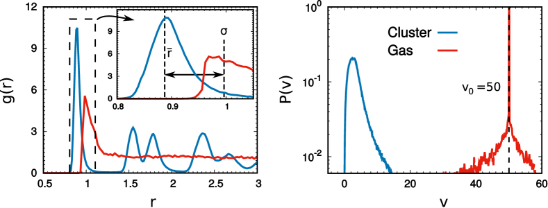
Figure 3: Panel (a): Pair correlation function, $g(r)$, computed within (blue) and outside (red) of the main cluster. The inset enlarges the first peak of the $g(r)$ as shown in the Figure. Panel (b): probability distribution function of the velocity, $p(v)$, within (blue) and out (red) of the main cluster. The observables are obtained from a simulation with $v_{0}=50$ and $D_{r}=0.2$. The other parameters are the same described in the main text.

In fig. 3 b), we also study the probability distribution function, $P(v)$, of the velocity modulus, $v=|\mathbf{v}|$, within (blue) and outside (red) of the cluster for a simulation with $v_{0}=50$ and $D_{r}=0.2$, displaying MIPS. Particles inside the cluster have a mean velocity, $\langle v\rangle$, slower than $v_{0}$, which is instead the typical speed value of particles in the disordered phase, as emerged by the presence of the large peak at $v=v_{0}$. We observe that a consistent fraction of particles in the disordered phase is not interaction-free as revealed by two tails for $v$ smaller and even larger $v_{0}$.

II The velocity of an Active Brownian particle: derivation of Eq.(4)

Eq. (1b) of the main text, i.e. the dynamics of the angle $\theta_{i}$, corresponds to the following vectorial equation for the associated orientation vector $\mathbf{n}_{i}$:

$$\dot{\mathbf{n}}_{i}=\sqrt{2D_{r}}\boldsymbol{\xi}_{i}\times\mathbf{n}_{i}\,,$$ (9)

being $\boldsymbol{\xi}_{i}$ a three dimensional vector with components $(0,0,\xi_{i})$ and $\langle\xi_{i}(t)\xi_{j}(t^{\prime})\rangle=\delta(t-t^{\prime})$, while $\mathbf{n}_{i}$ is a unit vector belonging to the $xy$-plane. In Eq. (9) the noise has multiplicative character and is integrated with the Stratonovich convention. Taking the time derivative of Eq. (1a) of the main text and defining $\mathbf{v}_{i}=\dot{\mathbf{x}}_{i}$, we get:

$$d\mathbf{v}_{i}=-\frac{1}{\gamma}\sum_{j}\nabla_{i}\nabla_{j}U_{tot}\cdot\mathbf{v}_{j}dt+v_{0}d\mathbf{n}_{i}\,.$$ (10)

In order to compute the variation $d\mathbf{n}_{i}$ we switch to Ito calculus and find after some standard manipulations:

$$d\mathbf{n}_{i}=\sqrt{2D_{r}}\,\boldsymbol{\xi}_{i}dt\times\mathbf{n}_{i}-D_{r}\mathbf{n}_{i}\,dt\,,$$ (11)

where by $\boldsymbol{\xi}_{i}dt$ we denote the Wiener process $d\boldsymbol{W}_{i}=\boldsymbol{\xi}_{i}dt$. Putting Eq. (11) into Eq. (10) we obtain:

$$d\mathbf{v}_{i}=-\frac{1}{\gamma}\sum_{j}\nabla_{i}\nabla_{j}U_{tot}\cdot\mathbf{v}_{j}dt-D_{r}v_{0}\mathbf{n}_{i}dt+v_{0}\sqrt{2D_{r}}\,\boldsymbol{\xi}_{i}dt\times\mathbf{n}_{i}\,.$$

Finally, using Eq. (1a), we get:

$$\frac{\gamma}{D_{r}}d\mathbf{v}_{i}=-\gamma\mathbf{v}_{i}dt-\frac{1}{D_{r}}\sum_{j}\nabla_{i}\nabla_{j}U_{tot}\cdot\mathbf{v}_{j}dt-\nabla_{i}U_{tot}dt+v_{0}\sqrt{2\frac{\gamma^{2}}{D_{r}}}\,\boldsymbol{\xi}_{i}dt\times\mathbf{n}_{i}\,.$$

Considering the definition of the matrix $\boldsymbol{\Gamma}$ given by Eq. (5) and $\mu=\gamma/D_{r}$, we obtain Eq. (4) of the main text.

III Effective equations for particles within the cluster: derivation of Eq.(6) and Eq.(7)

Let us start from Eq. (4) for a system of particles placed on a perfect hexagon, as in the bulk of the cluster. A target particle interacts only with its six neighbors at distance $\bar{r}<\sigma$ due to the the nature of the potential that cuts off the interactions with particles located at distances larger than $\sigma$. By symmetry, in Eq. (4) the external force contribution, $\mathbf{F}_{i}$, on the target particle, turns out to be zero and the only contribution to the dynamics comes from the noise source and from the velocities-dependent terms, $\sum_{j}\boldsymbol{\Gamma}_{ij}\cdot\mathbf{v}_{j}$, which explicitly read:

$$\sum_{j}\boldsymbol{\Gamma}_{ij}\cdot\mathbf{v}_{j} =\sum_{j}\mathbf{v}_{j}\cdot\left[\mathcal{I}+\frac{\gamma}{D_{r}}\nabla_{i}\nabla_{j}U_{tot}\right]$$ (12)

$$=\mathbf{v}_{i}+\frac{\gamma}{D_{r}}\sum_{j=1}^{6}\mathbf{v}_{i}\cdot\nabla_{i}\nabla_{i}U\left(r_{ij}\right)+\frac{\gamma}{D_{r}}\sum_{j=1}^{6}\mathbf{v}_{j}\cdot\nabla_{i}\nabla_{j}U\left(r_{ij}\right)\,,$$

being $r_{ij}$ the distance between the $i$-th and $j$-th particle. The last two terms of Eq. (12) can be explicitly evaluated by considering the derivative with respect to the spatial components denoted by Greek upper indices:

$$\nabla^{\alpha}_{i}\nabla^{\beta}_{i}U\left(r_{ij}\right)=\left[U^{\prime\prime}(r_{ij})+\frac{U^{\prime}(r_{ij})}{|r_{ij}|}\right]\frac{r_{ij}^{\alpha}r_{ij}^{\beta}}{|r_{ij}|^{2}}-\delta_{\alpha\beta}\frac{U^{\prime}(r_{ij})}{|r_{ij}|}\,,$$ (13)

being $r_{ij}^{\alpha}=r_{i}^{\alpha}-r_{j}^{\alpha}$, with $\alpha=x,y$. Denoting with $\delta_{j}$ the angle formed (with respect to the $x$-axis) between the $j$-th and the $i$-th particle, we can note that $r_{ij}^{\alpha}/|r_{ij}|$ reads $\cos{\left(\delta_{j}\right)}$ and $\sin{\left(\delta_{j}\right)}$ for $\alpha=x,y$, respectively. Since particles belong to a perfect hexagon we can express the angle as a function of $j$ in such a way that $\delta_{j}=\delta_{0}+j\pi/3$. The orientation of the hexagon with respect to the reference frame is fixed by the angle $\delta_{0}$, which we set to zero for the sake of simplicity. Expressing the matrix elements of Eq. (13) in terms of trigonometric functions, we get:

$$\hat{H}_{j}=\begin{pmatrix}U^{\prime\prime}(\bar{r})\cos^{2}(j\pi/3)+\frac{U^{\prime}(\bar{r})}{|\bar{r}|}\sin^{2}(j\pi/3)\;\;\;&\left[U^{\prime\prime}(\bar{r})-\frac{U^{\prime}(\bar{r})}{|\bar{r}|}\right]\cos(j\pi/3)\sin(j\pi/3)\\ \left[U^{\prime\prime}(\bar{r})-\frac{U^{\prime}(\bar{r})}{|\bar{r}|}\right]\cos(j\pi/3)\sin(j\pi/3)\;\;\;&U^{\prime\prime}(\bar{r})\sin^{2}(j\pi/3)+\frac{U^{\prime}(\bar{r})}{|\bar{r}|}\cos^{2}(j\pi/3)\end{pmatrix}.$$ (14)

Since the potential depends only on the inter-particle distance the following property holds:

$$\nabla^{\alpha}_{i}\nabla^{\beta}_{j}U=-\nabla^{\alpha}_{i}\nabla^{\beta}_{i}U\,,$$ (15)

and we can easily find Eq. (6) of the main text, assuming that $r_{ij}=\bar{r}$ for every $j$.

The derivation of Eq. (7) of the main text comes directly from Eq. (6) ibid., by separating the force $\propto\mathbf{v}$ from the one $\propto\mathbf{v}_{j}$. In particular, we observe that the sum over $j$ of the matrix element of $\hat{H}_{j}$ gives rise to a very simple shape in the hexagonal configuration:

$$\sum_{j=1}^{6}\hat{H}_{j}=3\left(U^{\prime\prime}+\frac{U^{\prime}}{\bar{r}}\right)\mathcal{I}\equiv\hat{J}\,.$$ (16)

Such a simplification comes from the following properties holding in general for every $\delta_{0}$:

$$\sum_{j=1}^{6}\cos^{2}{\left(\delta_{0}+\frac{j\pi}{3}\right)}=\sum_{j=1}^{6}\sin^{2}{\left(\delta_{0}+\frac{j\pi}{3}\right)}=3\,,$$ (17)

$$\sum_{j=1}^{6}\cos{\left(\delta_{0}+\frac{j\pi}{3}\right)}\sin{\left(\delta_{0}+\frac{j\pi}{3}\right)}=0\,.$$ (18)

Finally, adding and subtracting $J\cdot\mathbf{v}^{*}$, being $\mathbf{v}^{*}=\sum_{j=1}^{6}\mathbf{v}_{j}$, we obtain Eq. (7).

IV Modes analysis of the velocity field in the hexagonal lattice

In this Section, we derive Eq. (8) of the main text discussing the approximations involved. Let us start from Eq. (6) of the main text: Replacing the multiplicative noise term by the additive noise $\sqrt{2\gamma(\mu v_{0}^{2})}\boldsymbol{\xi}$ and applying the discrete Fourier transform to the corresponding equation we obtain

$$\mu\frac{\partial}{\partial t}\tilde{\mathbf{v}}(\mathbf{k},t)=-\gamma\tilde{\mathbf{v}}(\mathbf{k},t)-\frac{1}{D_{r}}\tilde{H}(\mathbf{k})\tilde{\mathbf{v}}(\mathbf{k},t)+\sqrt{2\gamma\mu v_{0}^{2}}\,\tilde{\boldsymbol{\xi}}(\mathbf{k},t)\,,$$ (19)

being $\tilde{\mathbf{v}}(\mathbf{k},t)$ and $\tilde{\boldsymbol{\xi}}(\mathbf{k},t)$ the Fourier transform of $\mathbf{v}$ and $\boldsymbol{\xi}$, respectively. The symmetric matrix $\tilde{H}(\mathbf{k})$, according to Eq. (14), has the following matrix elements

$$\tilde{H}_{xx}(\mathbf{k}) = \left(U^{\prime\prime}(\bar{r})+3\frac{U^{\prime}(\bar{r})}{\bar{r}}\right)\left[\cos(\frac{k_{x}\bar{r}}{2})\cos(\frac{\sqrt{3}k_{y}\bar{r}}{2})-1\right]+2\,U^{\prime\prime}(\bar{r})[\cos(k_{x}\bar{r})-1]\,,$$ (20)

$$\tilde{H}_{yy}(\mathbf{k}) = \left(3U^{\prime\prime}(\bar{r})+\frac{U^{\prime}(\bar{r})}{\bar{r}}\right)\left[\cos(\frac{k_{x}\bar{r}}{2})\cos(\frac{\sqrt{3}k_{y}\bar{r}}{2})-1\right]+2\frac{U^{\prime}(\bar{r})}{\bar{r}}\,[\cos(k_{x}\bar{r})-1]\,,$$ (21)

$$\tilde{H}_{xy}(\mathbf{k}) = \sqrt{3}\left(U^{\prime\prime}(\bar{r})+3\frac{U^{\prime}(\bar{r})}{\bar{r}}\right)\sin(\frac{k_{x}\bar{r}}{2})\sin(\frac{\sqrt{3}k_{y}\bar{r}}{2})\,.$$ (22)

Eq. (19) can be easily solved

$$\tilde{\mathbf{v}}(\mathbf{k},t)=\tilde{\mathbf{v}}(\mathbf{k},0)e^{-\alpha(\mathbf{k})t}+\sqrt{2\gamma\mu v_{0}^{2}}\,\int_{0}^{t}dt^{\prime}\,e^{-\alpha(\mathbf{k})(t-t^{\prime})}\,\tilde{\boldsymbol{\xi}}(\mathbf{k},t)\,,$$ (23)

where, for the sake of simplicity, we report $\alpha(\mathbf{k})$ in the small $k$ limit, obtaining:

$$\alpha(\mathbf{k})=D_{r}+\frac{3}{4\gamma}\left(U^{\prime\prime}(\bar{r})+\frac{U^{\prime}(\bar{r})}{\bar{r}}\right)\left|\mathbf{k}\right|^{2}\bar{r}^{2}\,.$$ (24)

The corresponding equal time velocity-correlation is

$$\langle\hat{v}_{x}(\mathbf{k},t)\hat{v}_{x}(-\mathbf{k},t)\rangle+\langle\hat{v}_{y}(\mathbf{k},t)\hat{v}_{y}(-\mathbf{k},t)\rangle=\frac{2v_{0}^{2}}{1+\lambda_{s}^{2}\left|\mathbf{k}\right|^{2}}\,,$$ (25)

where

$$\lambda_{s}\approx\bar{r}\left[\frac{3}{4}\frac{1}{\gamma D_{r}}\left(U^{\prime\prime}(\bar{r})+\frac{U^{\prime}(\bar{r})}{|\bar{r}|}\right)\right]^{1/2}\,.$$ (26)

The expression (26) corresponds to Eq. (8)of the main text. Coming back to the real space representation, Eq. (25) turns into:

$$\langle\mathbf{v}(\mathbf{x+r},t)\mathbf{v}(\mathbf{x},t)\rangle\approx 2v_{0}^{2}\Bigl{(}\frac{\lambda_{s}}{8\pi r}\Bigr{)}^{1/2}e^{-r/\lambda_{s}}\,.$$ (27)

We outline that the correlation length, Eq. (26), and the exponential shape of the space correlation, Eq. (27), are the results of the expansion for small $\mathbf{k}$.

V Forces contributions in the aligned and vortex domains

In this Section, we calculate the velocity dependent force on a target particle due to the six surrounding particles having velocities, $\mathbf{v}_{j}$, with $j=1,...,6$. The particle with $j=1$ is placed on the $x$ direction at coordinates $(\bar{r},0)$. The others are placed sequentially in the anti-clockwise sense at reciprocal angular distance $\pi/3$ and at distance $\bar{r}$ from the origin of the reference frame. We check that in the ideal cases of aligned domains and vortex structures the only relevant force contribution in Eq. (7) is the alignment term, $\propto\hat{J}\cdot(\mathbf{v}-\mathbf{v}^{*})$, while the other forces vanish or are irrelevant. Let us start from Eq. (7) of the main text, which we rewrite below, for completeness:

$$\mu\dot{\mathbf{v}}=-\frac{1}{D_{r}}\hat{J}\cdot(\mathbf{v}-\mathbf{v}^{*})+\frac{1}{D_{r}}\sum^{6}_{j=1}(\hat{H}_{j}-\frac{\hat{J}}{6})\cdot\mathbf{v}_{j}-\gamma\mathbf{v}+\sqrt{2\gamma(\mu v_{0}^{2})}\boldsymbol{\xi}\times{\mathbf{n}}\,,$$ (28)

The last two terms of the right-hand side of Eq. (28) are irrelevant in the large persistence regime, where $D_{r}$ is small. Instead, the second addend of the right-hand side of Eq. (28) needs to be computed:

$${\bf T}\equiv\frac{1}{D_{r}}\sum^{6}_{j=1}(\hat{H}_{j}-\frac{\hat{J}}{6})\cdot\mathbf{v}_{j}\,.$$ (29)

By symmetry, the contributions on T due to the particles placed at he opposite vertices of the hexagon are equal. Thus, in our notation, we have $H_{1}=H_{4}$, $H_{2}=H_{5}$ and $H_{3}=H_{6}$. Below, we write explicitly each term:

$$\hat{H}_{1}-\frac{\hat{J}}{6}=\hat{H}_{4}-\frac{\hat{J}}{6}=\left(U^{\prime\prime}(\bar{r})-\frac{U^{\prime}(\bar{r})}{\bar{r}}\right)\begin{pmatrix}-\frac{1}{4}\;\;\;&\frac{\sqrt{3}}{4}\\ \frac{\sqrt{3}}{4}\;\;\;&\frac{1}{4}\end{pmatrix}\,,$$ (30)

$$\hat{H}_{2}-\frac{\hat{J}}{6}=\hat{H}_{5}-\frac{\hat{J}}{6}=\left(U^{\prime\prime}(\bar{r})-\frac{U^{\prime}(\bar{r})}{\bar{r}}\right)\begin{pmatrix}-\frac{1}{4}\;\;\;&-\frac{\sqrt{3}}{4}\\ -\frac{\sqrt{3}}{4}\;\;\;&\frac{1}{4}\end{pmatrix}\,,$$ (31)

$$\hat{H}_{3}-\frac{\hat{J}}{6}=\hat{H}_{6}-\frac{\hat{J}}{6}=\left(U^{\prime\prime}(\bar{r})-\frac{U^{\prime}(\bar{r})}{\bar{r}}\right)\begin{pmatrix}\frac{1}{2}\;\;\;&0\\ 0\;\;\;&-\frac{1}{2}\end{pmatrix}\,.$$ (32)

Using the above expressions for $H_{j}$ we get:

$$T_{x} =\frac{1}{4D_{r}}\left(U^{\prime\prime}(\bar{r})-\frac{U^{\prime}(\bar{r})}{\bar{r}}\right)\left[2v_{6x}+2v_{3x}-v_{1x}-v_{2x}-v_{4x}-v_{5x}+\sqrt{3}(v_{1y}+v_{4y}-v_{2y}-v_{5y})\right]\,,$$ (33)

$$T_{y} =\frac{1}{4D_{r}}\left(\frac{U^{\prime}(\bar{r})-U^{\prime\prime}(\bar{r})}{\bar{r}}\right)\left[2v_{6y}+2v_{3y}-v_{1y}-v_{2y}-v_{4y}-v_{5y}+\sqrt{3}(v_{1x}+v_{4x}-v_{2x}-v_{5x})\right]\,.$$ (34)

Both components of the force vanish in the following cases: i) when all velocities are identical, i.e. in the case of aligned domains. ii) When the velocity of the six neighboring particles are arranged in a vortex configuration, for instance, described by the following velocity profile:

$${\mathbf{v}}_{j}=v_{0}\left[-\sin\left(j\frac{\pi}{3}\right),\cos\left(j\frac{\pi}{3}\right)\right]\,.$$ (35)

In this last case, the corresponding average velocity vaninshes, i.e. $\mathbf{v}^{*}=0$.

References

- Ward et al. (2008) A. J. Ward, D. J. Sumpter, I. D. Couzin, P. J. Hart, and J. Krause, Proceedings of the National Academy of Sciences 105, 6948 (2008).
- Ballerini et al. (2008) M. Ballerini, N. Cabibbo, R. Candelier, A. Cavagna, E. Cisbani, I. Giardina, V. Lecomte, A. Orlandi, G. Parisi, A. Procaccini, et al., Proceedings of the national academy of sciences 105, 1232 (2008).
- Attanasi et al. (2014) A. Attanasi, A. Cavagna, L. Del Castello, I. Giardina, S. Melillo, L. Parisi, O. Pohl, B. Rossaro, E. Shen, E. Silvestri, et al., Phys. Rev. Lett. 113, 238102 (2014).
- Mora et al. (2016) T. Mora, A. M. Walczak, L. Del Castello, F. Ginelli, S. Melillo, L. Parisi, M. Viale, A. Cavagna, and I. Giardina, Nat. Phys. 12, 1153 (2016).
- Cavagna et al. (2017) A. Cavagna, D. Conti, C. Creato, L. Del Castello, I. Giardina, T. S. Grigera, S. Melillo, L. Parisi, and M. Viale, Nat. Phys. 13, 914 (2017).
- Dell’Arciprete et al. (2018) D. Dell’Arciprete, M. Blow, A. Brown, F. Farrell, J. S. Lintuvuori, A. McVey, D. Marenduzzo, and W. C. Poon, Nat. Comm. 9, 4190 (2018).
- Berg (2008) H. Berg, E. Coli in Motion (Springer Science & Business Media, 2008).
- Peruani et al. (2012) F. Peruani, J. Starruß, V. Jakovljevic, L. Søgaard-Andersen, A. Deutsch, and M. Bär, Phys. Rev. Lett. 108, 098102 (2012).
- Petroff et al. (2015) A. P. Petroff, X.-L. Wu, and A. Libchaber, Phys. Rev. Lett. 114, 158102 (2015).
- Bialké et al. (2015a) J. Bialké, T. Speck, and H. Löwen, J. Non-Cryst. Solids 407, 367 (2015a).
- Palacci et al. (2013) J. Palacci, S. Sacanna, A. Steinberg, D. Pine, and P. Chaikin, Science , 1230020 (2013).
- Buttinoni et al. (2013) I. Buttinoni, J. Bialké, F. Kümmel, H. Löwen, C. Bechinger, and T. Speck, Phys. Rev. Lett. 110, 238301 (2013).
- Ginot et al. (2018) F. Ginot, I. Theurkauff, F. Detcheverry, C. Ybert, and C. Cottin-Bizonne, Nat. Comm. 9, 696 (2018).
- Yan et al. (2016) J. Yan, M. Han, J. Zhang, C. Xu, E. Luijten, and S. Granick, Nat. Mat. 15, 1095 (2016).
- Bricard et al. (2015) A. Bricard, J.-B. Caussin, D. Das, C. Savoie, V. Chikkadi, K. Shitara, O. Chepizhko, F. Peruani, D. Saintillan, and D. Bartolo, Nat. Comm. 6, 7470 (2015).
- Howse et al. (2007) J. R. Howse, R. A. L. Jones, A. J. Ryan, T. Gough, R. Vafabakhsh, and R. Golestanian, Phys. Rev. Lett. 99, 048102 (2007).
- Takatori et al. (2016) S. C. Takatori, R. De Dier, J. Vermant, and J. F. Brady, Nat. Comm. 7, 10694 (2016).
- Marchetti et al. (2013) M. C. Marchetti, J. F. Joanny, S. Ramaswamy, T. B. Liverpool, J. Prost, M. Rao, and R. A. Simha, Rev. Mod. Phys. 85, 1143 (2013).
- Ramaswamy (2010) S. Ramaswamy, Annu. Rev. Condens. Matter Phys. 1, 323 (2010).
- Bechinger et al. (2016) C. Bechinger, R. Di Leonardo, H. Löwen, C. Reichhardt, G. Volpe, and G. Volpe, Reviews of Modern Physics 88, 045006 (2016).
- Palacci et al. (2010) J. Palacci, C. Cottin-Bizonne, C. Ybert, and L. Bocquet, Phys. Rev. Lett. 105, 088304 (2010).
- Theurkauff et al. (2012) I. Theurkauff, C. Cottin-Bizonne, J. Palacci, C. Ybert, and L. Bocquet, Phys. Rev. Lett. 108, 268303 (2012).
- ten Hagen et al. (2011) B. ten Hagen, S. van Teeffelen, and H. Löwen, J. Phys. Condens. Matter 23, 194119 (2011).
- Romanczuk et al. (2012) P. Romanczuk, M. Bär, W. Ebeling, B. Lindner, and L. Schimansky-Geier, Eur. Phys. J. Special Topics 202, 1 (2012).
- Peruani et al. (2006) F. Peruani, A. Deutsch, and M. Bär, Physical Review E 74, 030904 (2006).
- Aranson and Tsimring (2003) I. S. Aranson and L. S. Tsimring, Physical Review E 67, 021305 (2003).
- Ginelli et al. (2010) F. Ginelli, F. Peruani, M. Bär, and H. Chaté, Phys. Rev. Lett. 104, 184502 (2010).
- Deseigne et al. (2010) J. Deseigne, O. Dauchot, and H. Chaté, Physical Review Letters 105, 098001 (2010).
- Vicsek and Zafeiris (2012) T. Vicsek and A. Zafeiris, Phys. Rep. 517, 71 (2012).
- Vicsek et al. (1995) T. Vicsek, A. Czirók, E. Ben-Jacob, I. Cohen, and O. Shochet, Phys. Rev. Lett. 75, 1226 (1995).
- Toner and Tu (1995) J. Toner and Y. Tu, Phys. Rev. Lett. 75, 4326 (1995).
- Toner (2012) J. Toner, Physical Review E 86, 031918 (2012).
- Mahault et al. (2018) B. Mahault, X.-c. Jiang, E. Bertin, Y.-q. Ma, A. Patelli, X.-q. Shi, and H. Chaté, arXiv preprint arXiv:1803.00104 (2018).
- Grégoire and Chaté (2004) G. Grégoire and H. Chaté, Phys. Rev. Lett. 92, 025702 (2004).
- Solon et al. (2015a) A. P. Solon, H. Chaté, and J. Tailleur, Phys. Rev. Lett. 114, 068101 (2015a).
- Caussin et al. (2014) J.-B. Caussin, A. Solon, A. Peshkov, H. Chaté, T. Dauxois, J. Tailleur, V. Vitelli, and D. Bartolo, Phys. Rev. Lett. 112, 148102 (2014).
- Lam et al. (2015) K.-D. N. T. Lam, M. Schindler, and O. Dauchot, New Journal of Physics 17, 113056 (2015).
- Giavazzi et al. (2018) F. Giavazzi, M. Paoluzzi, M. Macchi, D. Bi, G. Scita, M. L. Manning, R. Cerbino, and M. C. Marchetti, Soft matter 14, 3471 (2018).
- Gonnella et al. (2015) G. Gonnella, D. Marenduzzo, A. Suma, and A. Tiribocchi, Compt. Rend. Phys. 16, 316 (2015).
- Cates and Tailleur (2015) M. E. Cates and J. Tailleur, Annu. Rev. Condens. Matter Phys. 6, 219 (2015).
- Fily and Marchetti (2012) Y. Fily and M. C. Marchetti, Phys. Rev. Lett. 108, 235702 (2012).
- Sese-Sansa et al. (2018) E. Sese-Sansa, I. Pagonabarraga, and D. Levis, EPL (Europhysics Letters) 124, 30004 (2018).
- Barré et al. (2015) J. Barré, R. Chétrite, M. Muratori, and F. Peruani, Journal of Statistical Physics 158, 589 (2015).
- van der Linden et al. (2019) M. N. van der Linden, L. C. Alexander, D. G. Aarts, and O. Dauchot, arXiv preprint arXiv:1902.08094 (2019).
- Shi and Chaté (2018) X.-q. Shi and H. Chaté, arXiv preprint arXiv:1807.00294 (2018).
- Geyer et al. (2019) D. Geyer, D. Martin, J. Tailleur, and D. Bartolo, Physical Review X 9, 031043 (2019).
- Chaté et al. (2008) H. Chaté, F. Ginelli, G. Grégoire, F. Peruani, and F. Raynaud, The European Physical Journal B 64, 451 (2008).
- Redner et al. (2013) G. S. Redner, M. F. Hagan, and A. Baskaran, Phys. Rev. Lett. 110, 055701 (2013).
- Fodor et al. (2016) E. Fodor, C. Nardini, M. E. Cates, J. Tailleur, P. Visco, and F. van Wijland, Phys. Rev. Lett. 117, 038103 (2016).
- Caprini et al. (2018) L. Caprini, U. M. B. Marconi, and A. Vulpiani, Journal of Statistical Mechanics: Theory and Experiment 2018, 033203 (2018).
- Caprini et al. (2019a) L. Caprini, U. M. B. Marconi, and A. Puglisi, Sci. Rep. 9, 1386 (2019a).
- Marconi et al. (2016) U. M. B. Marconi, N. Gnan, M. Paoluzzi, C. Maggi, and R. Di Leonardo, Sci. Rep. 6, 23297 (2016).
- Yang et al. (2010) Y. Yang, V. Marceau, and G. Gompper, Phys. Rev. E 82, 031904 (2010).
- Bär et al. (2019) M. Bär, R. Großmann, S. Heidenreich, and F. Peruani, arXiv preprint arXiv:1907.00360 (2019).
- Suma et al. (2014) A. Suma, G. Gonnella, D. Marenduzzo, and E. Orlandini, EPL (Europhysics Letters) 108, 56004 (2014).
- Cugliandolo et al. (2017) L. F. Cugliandolo, P. Digregorio, G. Gonnella, and A. Suma, Phys. Rev. Lett. 119, 268002 (2017).
- Caprini et al. (2019b) L. Caprini, U. Marini Bettolo Marconi, A. Puglisi, and A. Vulpiani, The Journal of Chemical Physics 150, 024902 (2019b).
- Farage et al. (2015) T. F. F. Farage, P. Krinninger, and J. M. Brader, Phys. Rev. E 91, 042310 (2015).
- Rein and Speck (2016) M. Rein and T. Speck, Eur. Phys. J. E 39, 84 (2016).
- Tailleur and Cates (2008) J. Tailleur and M. E. Cates, Phys. Rev. Lett. 100, 218103 (2008).
- Cates and Tailleur (2013) M. Cates and J. Tailleur, EPL (Europhysics Letters) 101, 20010 (2013).
- Speck (2016) T. Speck, The European Physical Journal Special Topics 225, 2287 (2016).
- Solon et al. (2018a) A. P. Solon, J. Stenhammar, M. E. Cates, Y. Kafri, and J. Tailleur, New Journal of Physics 20, 075001 (2018a).
- Stenhammar et al. (2013) J. Stenhammar, A. Tiribocchi, R. J. Allen, D. Marenduzzo, and M. E. Cates, Phys. Rev. Lett. 111, 145702 (2013).
- Speck et al. (2014) T. Speck, J. Bialké, A. M. Menzel, and H. Löwen, Phys. Rev. Lett. 112, 218304 (2014).
- Solon et al. (2015b) A. P. Solon, Y. Fily, A. Baskaran, M. E. Cates, Y. Kafri, M. Kardar, and J. Tailleur, Nat. Phys. 11, 673 (2015b).
- Solon et al. (2015c) A. P. Solon, J. Stenhammar, R. Wittkowski, M. Kardar, Y. Kafri, M. E. Cates, and J. Tailleur, Phys. Rev. Lett. 114, 198301 (2015c).
- Bialké et al. (2015b) J. Bialké, J. T. Siebert, H. Löwen, and T. Speck, Phys. Rev. Lett. 115, 098301 (2015b).
- Patch et al. (2018) A. Patch, D. M. Sussman, D. Yllanes, and M. C. Marchetti, Soft Matter 14, 7435 (2018).
- Mandal et al. (2019) S. Mandal, B. Liebchen, and H. Löwen, arXiv preprint arXiv:1902.06116 (2019).
- Stenhammar et al. (2014) J. Stenhammar, D. Marenduzzo, R. J. Allen, and M. E. Cates, Soft Matter 10, 1489 (2014).
- Wittkowski et al. (2014) R. Wittkowski, A. Tiribocchi, J. Stenhammar, R. J. Allen, D. Marenduzzo, and M. E. Cates, Nat. Comm. 5, 4351 (2014).
- Tjhung et al. (2018) E. Tjhung, C. Nardini, and M. E. Cates, Phys. Rev. X 8, 031080 (2018).
- Großmann et al. (2019) R. Großmann, I. S. Aranson, and F. Peruani, arXiv preprint arXiv:1906.00277 (2019).
- Solon et al. (2018b) A. P. Solon, J. Stenhammar, M. E. Cates, Y. Kafri, and J. Tailleur, Phys. Rev. E 97, 020602(R) (2018b).
- Paoluzzi et al. (2019) M. Paoluzzi, C. Maggi, and A. Crisanti, arXiv preprint arXiv:1909.08462 (2019).