Bayesian stochastic multi-scale analysis via energy considerations

Abstract

In this paper physical multi-scale processes governed by their own principles for evolution or equilibrium on each scale are coupled by matching the stored and dissipated energy, in line with the Hill-Mandel principle. In our view the correct representations of stored and dissipated energy is essential to the representation irreversible material behaviour, and this matching is also used for upscaling. The small scales, here the meso-scale, is assumed to be described probabilistically, and so on the macroscale also a probabilistic model is identified in a Bayesian setting, reflecting the randomness of the meso-scale, the loss of resolution due to upscaling, and the uncertainty involved in the Bayesian process. In this way multi-scale processes become hierarchical systems in which the information is transferred across the scales by Bayesian identification on coarser levels. The quantities to be matched on the coarse-scale model are the stored and dissipated energies. In this way probability distributions of macro-scale material parameters are determined, and not only in the elastic region, but also for the irreversible and highly nonlinear elasto-damage regimes, refelcting the aleatory uncetainty at the meso-scale level. For this purpose high dimensional meso-scale stochastic simulations in a non-intrusive functional approximation forms are mapped to the macro-scale models in an approximative manner by employing a generalised version of the Kalman filter. To reduce the overall computational cost, a model reduction of the meso-scale simulation is achieved by combining the unsupervised learning techniques based on the Bayesian copula variartional inference with the classical functional approximation forms from the field of uncertainty quantification.

1 Introduction

The predictive modelling of concrete as a heterogeneous material requires more realistic mathematical models. This is especially true when describing the nonlinear material behaviour, which is not fully resolved unless observed on multiple scales going from nano-to macro-scale descriptions. As the detailed description on the macroscopic level is not computationally feasable for large scale structures, the multi-scale approaches are often utilised in the numerical practice. In this paper only macro- and meso-scale descriptions of concrete will be considered, however, lower scales can be introduced as well in order to explicitely describe heterogeneities characterising the material structure of aggregates, the mortar matrix or the interfacial zone without any further modifications.

Conceptually, the prevalent computational methods to tackle the multiscale problems can be classified into concurrent and non-concurrent approaches. Concurrent schemes consider both the coarse and fine-scales during the course of the simulation e.g. FE-squared method [12, 11], whereas the non-concurrent ones are based on a scale separation idea by which the desired quantity of interest (QoI), e.g. average stresses or strains, are estimated given numerical experiments on a representative volume element (RVE), see [16] for a recent overview on related techniques. Although, the non-concurrent method has proved to work very well for elastic properties, it does not explicitly include complex loading paths induced by structural effect, which are of crucial concern when dealing with material non-linearites such as plasticity and damage. In addition, the so-called size-effect problem, e.g. a problem of determining the size of the representative element, appears and has to be resolved. In (martan’s thesis) this is achieved by considering the mesh in element approach (MIEL) in which the meso-scale sturcture is embedded in a macro-scale finite element. Multi-scale here means an explicit distinction made between microscopic or micro variables – describing the fine scale representation – and macroscopic or macro variables – describing the coarser-scale.

The main problem in a multi-scale simulation is the process of bridging the scales, especially those of different nature, e.g. discrete versus continuum finite element descriptions on the meso-scale and macro-scale, respectivelly. In previous work, see [26], the infromation transfer is achieved in a Bayesian probabilistic manner. The meso-scale response is taken as measurement, and the properties of the macro-element are assumed to be unknown, and hence uncertain. As they cannot be directly measured, their estimation is obtained indirectly from the measurement data. Such an inversion is not well posed in a sense of Hadamard, and hence the regularisation is needed. In a Bayesian setting this matches with introducing the prior information, i.e. expert’s knowledge or epistemic uncertainty, onto the parameter set. This further results in an well-posed problem, the solution of which is stochastic and not deterministic any more. The resulting probability distributions are however only epistemic uncertainties and represent our confidence in obtained estimates. In this paper we go one step further and extend the previous approach, further reffered as the problem of stochastic upscaling, by including a proper treatment of aleatory uncertainties used to describe the meso-scale models. These are characterised by variations reflecting in uncertainties describing the geometry, the spatial distribution and the material properties of the individual material constituents and their mutual interaction.

Stochastic homogenization is usually performed on an ensemble of RVEs in order to extract the relevant statistical QoI [31, 27, 28, 30, 29, 37, 36, 42, 41, 43]. For example, in [18, 23], the moving-window approach is used to characterize the probabilistic uni-axial compressive strength of random micro-structures. Another active direction of research is to develop stochastic surrogate models for strain energy of random micro-structures as in [6, 8, 7, 40]. The main goal is to mitigate the effect of curse of dimensionality due to large number of stochastic dimensions. With the rapid expansion of machine learning and data driven techniques, the current trend is to train neural network based approximate models [24, 1, 35, 47, 48] as a cheaper computational alternative in multi-scale methods. Furthermore, to obtain a probabilistic description of macro-scale characteristic by incorporating micro-scale measurements, Bayesian methods have been applied to such problems with promising success, please see [13, 14, 15, 22, 5] for recent application in formulation of high dimensional probabilistic inverse problem generally, and estimating distribution of material parameter specifically. Moreover [21, 38, 10, 26] demonstrate the application of Bayesian framework to multi-scale problems.

This paper serves as an extension of the previously mentioned approaches. The idea is to design an appropriate macro-scale model, as well as its corresponding parameters such that the meso-scale energy is preserved. For this purpose the non-dissipative and dissipative parts of meso-scale strain energies are captured, and further used as measurements in the Bayesian estimation of the macro-scale properties. Here, three different kinds of algorithms are considered. The first addresses direct simulation of the probabilistic meso-scale model, which further results in a high-dimensional strain energy proxy model. The latter one is further mapped to the macro-scale parameter by using the generalised Gauss-Markov-Kalman filter as previously described in [32]. Even though the direct simulation allows for the deterministic estimates of the stochastic quantities when treated in a functional approximation setting, this approach is not attractive in real situations when only the meso-scale measurement data are available, or when the parameteric dimension of the model exponentially grows. Therefore, we present another upscaling version in which the non-dissipative and dissipative parts of meso-scale energy are sampled, and further mapped to its lower dimensional causin by an unsupervised data driven learning technique. The idea is to map the non-Guassian energy measurement to lower dimensional Gaussian space by a nonlinear mapping. Here this is achieved by emloying the copula based variational inference on a generalised mixture model. Due to high nonlinearity and history dependence such a mapping is not easy to construct, and therefore we employ additional Bayesian correction of the estimate in a sparse form. This is then contrasted to a more practical solution in which the upscaled parameters on the macro-scale level are sampled instead of energies, and further mapped to the lower dimensional Gaussian space. As further discussed this approach is computationally more convenient as the correlation structure between the material parameters is easier to learn.

The paper is organised as follows: in section 1 the generalised model problem is presented, and the research questions are defined. Section 2 describes Bayesian framework for upscaling random meso-scale information with the particular focus on the approximate posterior estimation. From computational point of view this is further discussed in Section 3. The process of model reduction of the meso-scale computations is further described in Section 4, whereas the energy conservation principle is discussed in Section 5. The algorithm performance is analysed in Section 6 on two different numerical examples, which are further concluded in Section 7.

2 Abstract model problem

Let $(\mathcal{Z}_{M},\mathcal{E}_{M},\mathcal{D}_{M})$ be an abstract structure of the general rate-independent small-strain homogeneous macro-model in which $\mathcal{Z}_{M}$ denotes the state space, $\mathcal{E}_{M}:[0,T]\times\mathcal{Z}_{M}\rightarrow\mathbb{R}$ is a time-dependent energy functional, and $\mathcal{D}_{M}:\mathcal{Z}_{M}\times\mathcal{Z}_{M}\rightarrow[0,\infty]$ is a convex and lower-semicontinuous dissipation potential satisfying $\mathcal{D}_{M}(z,0)=0$ and the homogeneity property $\forall z,y\in\mathcal{Z}_{M}:\textrm{ }\mathcal{D}_{M}(z,\lambda y)=\lambda\mathcal{D}_{M}(z,y)$ for all $\lambda>0$. Then, in an abstract manner the macro-mechanical system can be described mathematically by the sub-differential inclusion

$$z:[0,T]\rightarrow\mathcal{Z}:\quad\quad\partial_{\dot{z}}\mathcal{D}_{M}(\kappa,z,\dot{z})+\textrm{D}_{z}\mathcal{E}_{M}(t,\kappa,z)\ni 0$$ (1)

in which $\textrm{D}_{z}$ stands for the Gâteux partial differential with respect to the state variable $z$, and the derivative of $\mathcal{D}_{M}$ is given in terms of the set-valued sub-differential $\partial\mathcal{D}_{M}$ in the sense of the convex analysis, see [33]. Furthermore, we assume that the rate-independent system in Eq. (1) is parameterised by a vector $\kappa$ representing homogeneous material characteristics only. This parameterisation can be extended by including boundary conditions, loadings, etc. into the set. However, this situation will not be considered here.

Given mathematical description in Eq. (1), the goal is to find the unknown set $\kappa$ such that the structural response of the macro-scale model matches the response of the meso-scale model as well as possible. The latter one is taken as a more detailed description of the macro-scale counterpart–the one that accounts for material and geometrical heterogenieties at a lower-scale level, and hence represents the system that we can evaluate at possibly high cost. The meso-scale mathematical model reads

$$\partial_{\dot{z}_{m}}\mathcal{D}_{m}(z_{m},\kappa_{m},\dot{z}_{m})+\textrm{D}_{z}\mathcal{E}_{m}(t,\kappa_{m},z_{m})\ni 0,$$ (2)

and is subjected to the same boundary conditions and forcings as the one in Eq. (1) . Here, we assume that the state space $\mathcal{Z}_{m}$, the energy functional $\mathcal{E}_{m}$ and the dissipation potentials $\mathcal{D}_{m}$ have same form as before with the only difference that the material parameters $\kappa$ are given more realistic description $\kappa_{m}$, and are known. However, any other kind of model which allows a “measurement” resp. computation of stored and dissipated energies could be also used.

As $\mathcal{Z}_{M}\neq\mathcal{Z}_{m}$, the states $z_{M}$ and $z_{m}$ cannot be directly compared, and the two models are to be compared by some observables or measurements $y\in\mathcal{Y}$, where $\mathcal{Y}$ is typically some vector space like $\mathbb{R}^{m}$. In other words, let

$$y_{m}=Y_{m}(z_{m}(\kappa_{m},f_{m}))+\hat{\epsilon},$$ (3)

be the meso-scale observable (e.g. energy, stress or strain etc.) in which $Y_{m}$ describes the measurement operator, $f_{m}$ is the external excitiation and $\hat{\epsilon}$ respresents the measurement noise. On the other side, let

$$y_{M}=Y_{M}(\kappa,z_{M}(\kappa,f_{M}))$$ (4)

be the prediction of the same observation on the macro-scale level this time described by the measurement operator $Y_{M}$ and the external excitation $f_{M}$ of the same type as $f_{m}$. To incorporate the prediction of discrepancy $\hat{\epsilon}$ as in Eq. (3), one has to model $y_{M}$ as a noisy variant. For this purpose we introduce the probability space $(\varOmega_{\epsilon},\mathfrak{B}_{\epsilon},\mathbb{P}_{\epsilon})$ and add to $Y_{M}(\kappa,z_{M}(\kappa,f_{M}))$ the random variable $\epsilon(\omega_{\epsilon})\in L_{2}(\varOmega_{\epsilon},\mathfrak{B}_{\epsilon},\mathbb{P}_{\epsilon};\mathbb{R}^{d})$ that best describes our knowledge about $\hat{\epsilon}$. Hence, Eq. (11) becomes stochastic and reads

$$y_{M}(\omega_{\epsilon})=Y_{M}(\kappa,z_{M}(\kappa,f_{M}))+\epsilon(\omega_{\epsilon}).$$ (5)

Typically, $\epsilon(\omega_{\epsilon})$ is modelled as a zero-mean Gaussian random variable $\epsilon\sim\mathcal{N}(0,C_{\epsilon})$ with covariance $C_{\epsilon}$. However, other models for $\epsilon(\omega_{\epsilon})$ can also be introduced without modifying the general setting presented in this paper.

In variaty of literature the measurement in Eq. (3) is considered as deteriministic, e.g. the measurement is a function of the state $z_{m}$ characterised by one realisation of the heterogeneous material. This further defines the first problem of our consideration:

Problem 1.

Find deterministic $\kappa$ in Eq. (1) such that the predictions of Eq. (5) match those of Eq. (3) in a measurement sense.

However, in a real multi-scale analysis the parameters $\kappa_{m}$ in Eq. (2) vary, or are not fully known. Hence, the meso-scale model is characterised by aleatory and epistemic uncertainties, which have to be encountered into the modelling process. Taking the probabilistic view on uncertainty, we model $\kappa_{m}$ as a random variable/field in $L_{2}(\varOmega_{\kappa},\mathfrak{B}_{\kappa},\mathbb{P}_{\kappa};\mathcal{K}_{m})$ defined by mapping

$$\kappa_{m}(\omega_{\kappa}):=\kappa_{m}(x,\omega_{\kappa}):\mathcal{G}\times\varOmega_{\kappa}\mapsto\mathcal{K}_{m}.$$ (6)

Here, $\mathcal{K}_{m}$ is the parameter space which depends on the application. As a consequence, the evolution problem described by $(\mathcal{Z}_{m},\mathcal{E}_{m},\mathcal{D}_{m})$ also becomes uncertain, and hence Eq. (2) rewrites to

$$\partial_{\dot{z}_{m}}\mathcal{D}_{m}(z_{m}(\omega_{\kappa}),\kappa_{m}(\omega_{\kappa}),\dot{z}_{m}(\omega_{\kappa}))+\textrm{D}_{z}\mathcal{E}_{m}(t,\omega,\kappa_{m}(x,\omega_{\kappa}),z_{m}(\omega_{\kappa}))\ni 0\textrm{ a.s.}$$ (7)

in which

$$\mathcal{E}_{m}(t,z_{m}(\omega_{\kappa}))=\int_{\varOmega_{\kappa}}\mathcal{E}_{m}(\kappa_{m}(x,\omega_{\kappa}),z_{m}(\omega_{\kappa}))\mathbb{P}(d\omega_{\kappa}),$$

$$\mathcal{D}_{m}(z_{m}(\omega_{\kappa}),\dot{z}_{m}(\omega_{\kappa}))=\int_{\varOmega_{\kappa}}\mathcal{D}_{m}(\kappa_{m}(\omega_{\kappa}),z_{m}(\omega_{\kappa}),\dot{z}_{m}(\omega_{\kappa}))\mathbb{P}(d\omega_{k}),$$ (8)

respectively.

Once the uncertainty is present in the meso-scale model, the observation in Eq. (3) rewrites to

$$y_{m}(\omega_{y})=Y_{m}(z_{m}(\kappa_{m}(\omega_{\kappa}),f_{m}(\omega_{\kappa})))+\hat{\epsilon}(\omega_{e}),\quad\omega_{y}:=(\omega_{\kappa},\omega_{e})$$ (9)

in which both the model and the error $\hat{\epsilon}(\omega_{e})\in L_{2}(\varOmega_{e},\mathfrak{B}_{e},\mathbb{P}_{e};\mathbb{R}^{d})$ are stochastic. This in turn modifes Problem 1 into

Problem 2.

Find stochastic $\kappa_{M}$ in Eq. (1) such that the predictions of Eq. (5) match those of Eq. (9) in a measurement sense.

The upscaling process that is related to Problem 1 is already considered in [26], and hence will not be repeated here. However, as we show later this problem is a special case of Problem 2 that is the main topic of this paper.

3 Bayesian upscaling of random mesostructures

Let the meso-scale parameter set $\kappa_{m}(\omega_{\kappa})$ define the observations in Eq. (9), here assumed to be continous. The goal is to use information in Eq. (9) in order to calibrate (upscale) the set of material parameters $\kappa$ of the coarse-scale model in Eq. (1). To achieve this, $\kappa$ is assumed to be uncertain (unknown) and further modelled a priori as a random variable $\kappa(\omega)$ —prior—belonging to $L_{2}(\Omega,\mathcal{F},\mathbb{P};\mathcal{K})$. Hence, the model in Eq. (1) rewrites to

$$\partial_{\dot{z}}\mathcal{D}_{M}(\kappa(\omega),z(\kappa(\omega)),\dot{z}(\kappa(\omega)))+\textrm{D}_{z}\mathcal{E}_{M}(t,\kappa(\omega),z(\kappa(\omega)))\ni 0,$$ (10)

and subsequentually a priori prediction of the macro-scale measurement becomes

$$y_{M}(\kappa(\omega),\epsilon(\omega_{\epsilon}))=Y_{M}(\kappa(\omega),z_{M}(\kappa(\omega)),f_{M}))+\epsilon(\omega_{\epsilon})$$ (11)

with $\epsilon(\omega_{\epsilon})\in L_{2}(\varOmega_{\epsilon},\mathfrak{B}_{\epsilon},\mathbb{P}_{\epsilon})$. The goal is to identify the vector $\kappa(\omega)$ given $y_{m}$ using Bayes’s rule such that

$$p(\kappa|y_{m})=\frac{p(y_{m}|\kappa)p(\kappa)}{p(y_{m})}$$ (12)

holds. As $\kappa$ is positive definite, this constraint has to be taken into consideration. Therefore, instead of Problem 1 and Problem 2 we consider their modified versions:

Problem 3.

Find deterministic $q:=\textrm{log }\kappa$ in Eq. (1) such that the predictions of Eq. (5) match those of Eq. (3) in a measurement sense.

and

Problem 4.

Find stochastic $q:=\textrm{log }\kappa$ in Eq. (1) such that the predictions of Eq. (5) match those of Eq. (9) in a measurement sense.

Instead of calibrating the vector $\kappa$ directly, we calibrate its logartithm as in this way computationally whatever approximations or linear operations are performed on the numerical representation of $q(x,\omega)$, in the end $\textrm{exp}(q(x,\omega))$ is always going to be positive. Additionally, the multiplicative group of positive real numbers—a (commutative) one-dimensional Lie group—is thereby put into correspondence with the additive group of reals, which also represents the (one-dimensional) tangent vector space at the group unit, the number one. This is the corresponding Lie algebra. A positive quadratic form on the Lie algebra—in one dimension necessarily proportional to Euclidean distance squared—can thereby be carried to a Riemannian metric on the Lie group. Therefore,

$$p(q|y_{m})=\frac{p(y_{m}|q)p(q)}{p(y_{m})}.$$ (13)

However, in practice the estimation of the full posterior $p(q|y_{m})$ is not analytically tractable. Numerical estimation on the other hand is expensive either due to evidence estimation or due to slow convergence of the random walk algorithms. As in engineering practice one is often not interested in estimating the full posterior measure, in this paper we investigate the estimation of the posterior functional given in a form of conditional expectation

$$\mathbb{E}(q|y_{m})=\int_{\varOmega}qp(q|y_{m})dq$$ (14)

as it is computationally simpler. Instead of direct intergation over the posterior measure, the conditional expectation can be straightforwardly estimated by projecting the random variable $q$ onto the subspace generated by the sub-sigma algebra $\mathfrak{B}:=\sigma(Y)$ of measurement. To achieve this, one has to compute the minimal distance of $q$ to the point $q^{*}$ which can be achieved in different ways. As shown by [2, 34], the notion of distance can be generalised given a strictly convex, differentiable function $\varphi:\mathbb{R}^{d}\mapsto\mathbb{R}$ with the hyperplane tangent $\mathcal{H}_{\hat{q}}(q)=\varphi(\hat{q})+\langle q-\hat{q},\nabla\varphi(\hat{q})\rangle$ to $\varphi$ at point $\hat{q}$, such that

$$q^{*}:=\mathbb{E}(q|\mathfrak{B})=\underset{\hat{q}\in L_{2}(\varOmega,\mathcal{B},\mathbb{P};\mathcal{Q})}{\arg\min}\textrm{}\mathbb{E}(\mathcal{D}_{\varphi}(q||\hat{q}))$$ (15)

holds. Here, $\mathcal{D}_{\varphi}(q||\hat{q})=\mathcal{H}_{q}(q)-\mathcal{H}_{\hat{q}}(q)$ denotes the distance term that is also known as the Bregman’s loss function (BLF) or divergence. In general the projection in Eq. (15) is of non-orthogonal kind and reflects the generalised inequality

$$\mathbb{E}(D_{\varphi}(q||\check{q}))\geq\mathbb{E}(D_{\varphi}(q||q^{*}))+\mathbb{E}(D_{\varphi}(q^{*}||\check{q}))$$ (16)

that also holds for any arbitrary $\mathfrak{F}$-measurable random variable $\check{q}$. In case when $q^{*}=\mathbb{E}(q)$ the previous relation rewrites to

$$\mathbb{E}(\mathcal{D}_{\varphi}(q||\mathbb{E}(q)))=\mathbb{E}(\mathcal{D}_{\varphi}(q||\check{q}))-\mathbb{E}(\mathcal{D}_{\varphi}(\mathbb{E}(q)||\check{q}))\geq 0,$$ (17)

in which the distance $\mathbb{E}(\mathcal{D}_{\varphi}(q||\mathbb{E}(q)))$ has notion of variance, further refered as Bregman’s variance. In terms of convex function $\varphi$ the Bregman’s variance obtains the following form

$$\textrm{var}_{\varphi}(q): = \mathbb{E}(\mathcal{D}_{\varphi}(q||\mathbb{E}(q)))=\mathbb{E}(\varphi(q)-\varphi(\mathbb{E}(q))+\langle q-\mathbb{E}(q),\nabla\varphi(\mathbb{E}(q))\rangle)$$ (18)

$$= \mathbb{E}(\varphi(q))-\varphi(\mathbb{E}(q))\geq 0,$$

which is also matching the definition of Jensen’s inequality in the context of the probability theory. By minimising the Bregmann’s variance in the last expression, one obtains the mean as the corresponding minimumm. Subsequentually, one may conclude that the mean is the same minimum point for any expected Bregman divergence, e.g.

$$\mathbb{E}(q)=\underset{\hat{q}\in L_{2}(\varOmega,\mathcal{F},\mathbb{P};\mathcal{Q})}{\arg\min}\mathbb{E}(\mathcal{D}_{\varphi}(q||\hat{q})).$$ (19)

Notice that similar can be derived for $\mathfrak{B}$-measurable random variables. The last relation then matches Eq. (15).

For computational purposes, the Bregman’s distance in Eq. (15) is further taken as the squared Euclidean distance by assuming $\varphi(q)=\frac{1}{2}q^{2}$, such that $\mathcal{D}_{\varphi}(q||\hat{q})=\frac{1}{2}\|q-\hat{q}\|^{2}$ and

$$q^{*}:=\mathbb{E}(q|\mathfrak{B})=\underset{\hat{q}\in L_{2}(\varOmega,\mathcal{B},\mathbb{P};\mathcal{Q})}{\arg\min}\textrm{}\mathbb{E}(\|q-\hat{q}\|^{2}).$$ (20)

In this manner Eq. (16) reduces to the Pythagorean theorem

$$\|q-\hat{q}\|^{2}=\|q-q^{*}\|^{2}+\|q^{*}-\hat{q}\|^{2}$$ (21)

in which by taking $q^{*}=\mathbb{E}(q|\mathcal{B})$ one obtains

$$\|q-\hat{q}\|^{2}=\|q-\mathbb{E}(q|\mathcal{B})\|^{2}+\|\mathbb{E}(q|\mathcal{B})-\hat{q}\|^{2}.$$ (22)

Integrating over the probability measure of $q$, the previous equality can be rewritten as inequality:

$$\mathbb{E}(\|q-\hat{q}\|^{2})\geq\mathbb{E}(\|q-\mathbb{E}(q|\mathcal{B})\|^{2})$$ (23)

which shows that the conditional expectation is the minimiser of the mean squared error. In addition, if $\hat{q}=\mathbb{E}(q)$ then it is also the minimum variance unbiased estimator.

3.1 Upscaling based on the conditional expectation approximation

Following Eq. (20), one may decompose the random variable $q$ belonging to $(\varOmega,\mathfrak{F},\mathbb{P})$ into projected $q_{p}$ and residual $q_{r}$ components such that

$$q=q_{p}+q_{o}=P_{\mathfrak{B}}q+(I-P_{\mathfrak{B}})q$$ (24)

holds. Here, $q_{p}=P_{\mathfrak{B}}q=\mathbb{E}(q|\mathfrak{B})$ is the orthogonal projection of the random variable $q$ onto the space $(\varOmega,\mathfrak{B},\mathbb{P})$ of all distributions consistent with the data, whereas $q_{o}:=(I-P_{\mathfrak{B}})q$ is its orthogonal residual. To give Eq. (24) more practical form, the projection term $P_{\mathfrak{B}}q$ is further described by a measurable mapping $\phi:y\mapsto q$ according to the Doob-Dynkin lemma which states:

$$\mathbb{E}(q|y)=\phi(y(q))=\phi\circ y\circ q.$$ (25)

As a result, Eq. (24) rewrites to:

$$q=\phi(y(q))+(q-\phi(y(q)))$$ (26)

in which the first term in the sum, i.e. $\phi(y(q))$, is taken to be the projection of $q$ onto the meso-scale data set $y_{m}$, whereas $(q-\phi(y(q)))$ is the residual component defined by a priori knowledge $q_{f}$. Following this, Eq. (26) recasts to the update equation for the random variable $q$ as

$$q_{a}=q_{f}+\phi(y_{m})-\phi(y_{M})$$ (27)

in which $y_{M}$ (see Eq. (5)) is the random variable representing our prior prediction/forecast of the measurement data, and $q_{a}$ is the assimilated random variable. Therefore, to estimate $q_{a}$ one requires only information on the map $\phi$.

For the sake of computational simplicity, the map in Eq. (25) is further approximated in a Galerkin manner by

$$\mathcal{Q}_{n}=\{\phi(y)\in\mathcal{Q}\textrm{ }|\textrm{ }\phi_{n}:y\rightarrow q\textrm{ a n-th degree polynomial}\}$$ (28)

such that the filter in Eq. (27) rewrites to

$$q_{a}(\omega)=q_{f}(\omega)+\phi_{n}(y_{m})-\phi_{n}(y_{M}).$$ (29)

As the map in Eq. (28) is parametrised by a set of coefficients $\beta$, i.e. $\phi_{n}(y;\beta)$, these further can be found by minimising the residual component (the optimality condition in Eq. (20)):

$$\beta^{*}=\underset{\beta}{\arg\min}\textrm{ }\mathbb{E}(\|q_{f}-\phi_{n}(y_{M};\beta)\|^{2}).$$ (30)

In an affine case, when $n=1,\phi_{1}(y_{M};\beta)=Ky+b$, the previous optimisation outcomes in a formula defining the well-known Kalman gain:

$$K=\textrm{cov}_{q_{f},y_{M}}\textrm{cov}_{y_{M}}^{-1}$$ (31)

such that the update formula in Eq. (29) reduces to the generalisation of the Kalman filter

$$q_{a}=q_{f}+K(y_{m}-y_{M}),$$ (32)

here refered as Gauss-Markov-Kalman filter, for more details please see [32].

However, in most of practical situations one has to deal with the nonlinearity of the measurement-parameter map, and in such a case the formula given in Eq. (32) is not optimal. One example is the process of upscaling in which the energy observation is used to predict the material characteristics. To overcome this issue, one may introduce higher order terms in the approximation in Eq. (28) either in a monomial form

$$\phi(y;\beta)=\sum_{i=0}^{p}K_{i}(y^{\vee i}),\quad\beta:=(K_{i})$$ (33)

in which $y^{\vee i}:=\textrm{Sym}(y^{\otimes i})$ is the symmetric tensor product of $y$ taken $i$ times with itself, or in a polynomial one

$$\phi(y;\beta)=\sum_{\alpha\in\mathcal{I}}K^{(\alpha)}V_{\alpha}(y)$$ (34)

in which $\mathcal{I}$ is the multi-index set with elements $\alpha:=(\alpha_{1},...,\alpha_{n})$, and $V_{\alpha}$ are multivariate polynomials possibly of orthogonal kind. Following this, one may distingusih the monomial filtering formula

$$q_{a}=q_{f}+\sum_{i=0}^{p}K_{i}(y_{m}^{\vee i}-y_{M}^{\vee i})$$ (35)

from the polynomial one

$$q_{a}=q_{f}+\sum_{\alpha\in\mathcal{I}}K^{(\alpha)}(V_{\alpha}(y_{m})-V_{\alpha}(y_{M})).$$ (36)

Note that the form of Eq. (36), given in monomials, is numerically not a good form—except for very low orders $n$ —and hence straightforward use in computations is not recommended.

Finally, in a similar manner as before one may estimate the unknown coefficients $\beta$ given the stationarity or orthogonality condition in Eq. (30). The uniquness of the solution as well as different forms of approximations are studied in [32].

3.1.1 Bayesian Gauss-Markov-Kalman filter

The filter presented in the previous section is known to be computationally expensive when the dimension of $q_{f}$ and $y_{M}$ is high. Therefore, one may substitute $y_{M}$ by a surrogate model

$$\hat{y}_{M}=\phi_{f}(q_{f};\beta)$$ (37)

in which $\phi_{f}$ is usually taken to be of polynomial type in arguments $q_{f}$ with the coefficients $\beta$. To estimate $\beta$ one may use the same type of estimator as described in the previous section, however, in a slightly different form, as this time one estimates the map $q_{f}\mapsto y_{M}$, i.e.

$$\beta^{*}=\underset{\beta}{\arg\min}\textrm{ }\mathbb{E}(\|y_{M}-\phi_{f}(q_{f};\beta)\|^{2})$$ (38)

as further described in details in [34] on an example of ordinary differential equation. However, the estimate provided by Eq. (38) requires the knowledge of the random variable $y_{M}$. Although we may estimate $y_{M}$ by propagating forward the uncertainty through the meso-scale model, this is not very efficient due to the high-dimensionality of the problem. Therefore, we assume that $y_{M}$ is in general only known as a set of samples, and our goal is to match $\hat{y}_{M}$ with $y_{M}$ in a distribution sense. To achieve this, we consider another type of Bregman’s divergence in which $\varphi(y)=\mathbb{E}(\pi_{y}\textrm{log }\pi_{y})$ is the continous entropy with $\pi_{y}$ being the density distribution of the random variable $y$. In such a case Eq. (38) rewrites to

$$\beta^{*}=\underset{\hat{y}_{M}:=\phi_{f}(q,\beta)}{\arg\min}\textrm{ }D_{KL}(y_{M}||\hat{y}_{M})$$ (39)

with

$$D_{KL}(y_{M}||\hat{y}_{M}):=\int\pi_{y_{M}}\textrm{ log }\frac{\pi_{y_{M}}}{\pi_{\hat{y}_{M}}}dy_{M}$$ (40)

being the Kullback-Leibler (KL) divergence, i.e. the distance betwen the prior variable $y_{M}$ and its approximation $\hat{y}_{M}$ obtained by propagation of $q_{f}$ to $y_{M}$ via nonlinear map $\phi_{f}(q_{f},\beta)$ parameterised by $\beta$. However, as the backward map $\phi_{f}$ is not explicitely known, one may approximate $\pi_{\hat{y}_{M}}$ by conditional density $\pi_{\hat{y}_{M}|x}$ coming from Bayes’s rule, see [34]

$$\pi_{\hat{y}_{M}|x}=\frac{\pi_{\hat{y}_{M},x}}{p_{x}}$$ (41)

in which $x:=(q_{f}(\omega_{i}),y_{M}(\omega_{i}))_{i=1}^{N}$ is the full set of data (samples) describing the forward propagation of $q_{f}$ to $y_{M}$. In order to specify $\hat{y}_{M}$ the only thing we need to find are the coefficients of the map $\phi_{f}$. Therefore, we infer $\beta$ given data $x$ using Bayes’s rule

$$p(\beta|x)=\frac{p(x,\beta)}{\int p(x,\beta)d\beta}$$ (42)

instead of Eq. (41). In general case the marginalisation in Eq. (42) can be expensive, and therefore in this paper we use the variational Bayesian inference instead. The idea is to introduce a family $\mathcal{D}:=\{g(\beta):=g(\beta|\lambda,w)\}$ over $\beta$ indexed by a set of free parameters $(w,\lambda)$ such that $\hat{y}_{M}\sim y_{M}$. Thus, the idea is to optimise the parameter values by minimising the Kullback-Leibler divergence

$$g^{*}(\beta)=\underset{g(\beta)\in\mathcal{D}}{\arg\min\textrm{ }}D_{KL}(g(\beta)||p(\beta|x))=\underset{g(\beta)\in\mathcal{D}}{\arg\min}\int g(\beta)\textrm{log }\frac{g(\beta)}{p(\beta|x)}d\beta$$ (43)

instead of Eq. (39). After few derivation steps as depicted in [25], the previous minimisation problem reduces to

$$\beta^{*}=\arg\max\mathcal{L}(g(\beta)):=\mathbb{E}_{g}(\textrm{log }p(x,\beta))-\mathbb{E}_{g}(\textrm{log }g(\beta))$$ (44)

in which $\mathcal{L}(g)$ is the evidence lower bound (ELBO), or variational free energy. To obtain closed-form solution for $\beta^{*}$, the usual practice is to assume that both posterior $p(\beta|x)$ as well as its approximation $g(\beta)$ can be factorised in a mean sense, i.e.

$$p(\beta|x)=\prod p(\beta_{i}|x),\quad g(\beta)=\prod g(\beta_{i})$$ (45)

in which each factor $p(\beta_{i}|x)$, $g(\beta_{i})$ is independent and belongs to the exponential family. Similarly, their complete conditionals given all other variables and observations are also assumed to belong to the exponential families and are assumed to be independent. Obviously these assumptions lead to conjugacy relationships, and closed form solution of Eq. (44) as further discussed in more detail in [25].

3.2 Upscaling based on the polynomial chaos approximation

To discretise RVs in Eq. (32), Eq. (35) and Eq. (36) we use functional approximations. This means that all RVs, say $y_{M}(\omega)$, are described as functions of known RVs $\{\theta_{1}(\omega),\dots,\theta_{n}(\omega),\dots\}$. Often, when for example stochastic processes or random fields are involved, one has to deal here with infinitely many RVs, which for an actual computation have to be truncated to a finte vector $\mathchoice{\displaystyle\boldsymbol{\theta}}{\textstyle\boldsymbol{\theta}}{\scriptstyle\boldsymbol{\theta}}{\scriptscriptstyle\boldsymbol{\theta}}(\omega)=[\theta_{1}(\omega),\dots,\theta_{L}(\omega)]\in\varTheta\cong\mathbb{R}^{L}$ of significant RVs. We shall assume that these have been chosen such as to be independent, and often even normalised Gaussian and independent. The reason to not use $q_{f}$ directly is that in the process of identification of $q$ they may turn out to be correlated, whereas $\mathchoice{\displaystyle\boldsymbol{\theta}}{\textstyle\boldsymbol{\theta}}{\scriptstyle\boldsymbol{\theta}}{\scriptscriptstyle\boldsymbol{\theta}}$ can stay independent as they are.

To actually describe the functions $y_{M}(\mathchoice{\displaystyle\boldsymbol{\theta}}{\textstyle\boldsymbol{\theta}}{\scriptstyle\boldsymbol{\theta}}{\scriptscriptstyle\boldsymbol{\theta}}),q_{f}(\mathchoice{\displaystyle\boldsymbol{\theta}}{\textstyle\boldsymbol{\theta}}{\scriptstyle\boldsymbol{\theta}}{\scriptscriptstyle\boldsymbol{\theta}})$, one further chooses a finite set of linearly independent functions $\{\Psi_{\alpha}\}_{\alpha\in\mathcal{J}_{Z}}$ of the variables $\mathchoice{\displaystyle\boldsymbol{\theta}}{\textstyle\boldsymbol{\theta}}{\scriptstyle\boldsymbol{\theta}}{\scriptscriptstyle\boldsymbol{\theta}}(\omega)$, where the index $\alpha=(\dots,\alpha_{k},\dots)$ often is a multi-index, and the set of multi-indices for approximation $\mathcal{J}_{Z}$ is a finite set with cardinality (size) $Z$. Many different systems of functions can be used, classical choices are [49, 17, 50] multivariate polynomials — leading to the polynomial chaos expansion (PCE) or generalised PCE (gPCE) [50], kernel functions, radial basis functions, or functions derived from fuzzy sets. The particular choice is immaterial for the further development. But to obtain results which match the above theory as regards $\mathscr{L}$-invariant subspaces, we shall assume that the set $\{\Psi_{\alpha}\}_{\alpha\in\mathcal{J}_{Z}}$ includes all the linear functions of $\mathchoice{\displaystyle\boldsymbol{\theta}}{\textstyle\boldsymbol{\theta}}{\scriptstyle\boldsymbol{\theta}}{\scriptscriptstyle\boldsymbol{\theta}}$. This is easy to achieve with polynomials, and w.r.t kriging it corresponds to universal kriging. All other functions systems can also be augmented by a linear trend.

Thus a RV $\mathchoice{\displaystyle\boldsymbol{y}}{\textstyle\boldsymbol{y}}{\scriptstyle\boldsymbol{y}}{\scriptscriptstyle\boldsymbol{y}}_{M}(\mathchoice{\displaystyle\boldsymbol{\theta}}{\textstyle\boldsymbol{\theta}}{\scriptstyle\boldsymbol{\theta}}{\scriptscriptstyle\boldsymbol{\theta}})$ would be replaced by a functional approximation — this gives these methods its name, sometimes also termed spectral approximation —

$$\mathchoice{\displaystyle\boldsymbol{y}}{\textstyle\boldsymbol{y}}{\scriptstyle\boldsymbol{y}}{\scriptscriptstyle\boldsymbol{y}}_{M}(\mathchoice{\displaystyle\boldsymbol{\theta}}{\textstyle\boldsymbol{\theta}}{\scriptstyle\boldsymbol{\theta}}{\scriptscriptstyle\boldsymbol{\theta}})=\sum_{\alpha\in\mathcal{J}_{Z}}\mathchoice{\displaystyle\boldsymbol{y}}{\textstyle\boldsymbol{y}}{\scriptstyle\boldsymbol{y}}{\scriptscriptstyle\boldsymbol{y}}_{M}^{(\alpha)}\Psi_{\alpha}(\mathchoice{\displaystyle\boldsymbol{\theta}}{\textstyle\boldsymbol{\theta}}{\scriptstyle\boldsymbol{\theta}}{\scriptscriptstyle\boldsymbol{\theta}})=\mathchoice{\displaystyle\boldsymbol{y}}{\textstyle\boldsymbol{y}}{\scriptstyle\boldsymbol{y}}{\scriptscriptstyle\boldsymbol{y}}_{M}(\mathchoice{\displaystyle\boldsymbol{\theta}}{\textstyle\boldsymbol{\theta}}{\scriptstyle\boldsymbol{\theta}}{\scriptscriptstyle\boldsymbol{\theta}}),$$ (46)

and analogously $\mathchoice{\displaystyle\boldsymbol{q}}{\textstyle\boldsymbol{q}}{\scriptstyle\boldsymbol{q}}{\scriptscriptstyle\boldsymbol{q}}_{f}$ by

$$\mathchoice{\displaystyle\boldsymbol{q}}{\textstyle\boldsymbol{q}}{\scriptstyle\boldsymbol{q}}{\scriptscriptstyle\boldsymbol{q}}_{f}(\mathchoice{\displaystyle\boldsymbol{\theta}}{\textstyle\boldsymbol{\theta}}{\scriptstyle\boldsymbol{\theta}}{\scriptscriptstyle\boldsymbol{\theta}})=\sum_{\alpha\in\mathcal{J}_{Z}}\mathchoice{\displaystyle\boldsymbol{q}}{\textstyle\boldsymbol{q}}{\scriptstyle\boldsymbol{q}}{\scriptscriptstyle\boldsymbol{q}}_{f}^{(\alpha)}\Psi_{\alpha}(\mathchoice{\displaystyle\boldsymbol{\theta}}{\textstyle\boldsymbol{\theta}}{\scriptstyle\boldsymbol{\theta}}{\scriptscriptstyle\boldsymbol{\theta}}).$$ (47)

Like always, there are several alternatives to determine the coefficients $\mathchoice{\displaystyle\boldsymbol{q}}{\textstyle\boldsymbol{q}}{\scriptstyle\boldsymbol{q}}{\scriptscriptstyle\boldsymbol{q}}_{f}^{(\alpha)},\mathchoice{\displaystyle\boldsymbol{y}}{\textstyle\boldsymbol{y}}{\scriptstyle\boldsymbol{y}}{\scriptscriptstyle\boldsymbol{y}}_{M}^{(\alpha)}$ in the previous equations. In this paper, they are estimated in a data-driven way by using the variational method presented in Section 3.1.1. Namely, Eq. (46) is taken as an example of Eq. (37) in which the coefficients $\mathchoice{\displaystyle\boldsymbol{v}}{\textstyle\boldsymbol{v}}{\scriptstyle\boldsymbol{v}}{\scriptscriptstyle\boldsymbol{v}}:=\{\mathchoice{\displaystyle\boldsymbol{y}}{\textstyle\boldsymbol{y}}{\scriptstyle\boldsymbol{y}}{\scriptscriptstyle\boldsymbol{y}}_{M}^{(\alpha)}\}_{\alpha\in\mathcal{J}_{Z}}$ are estimated by minimising ELBO analogous to the one in Eq. (44) by using the variational relevance vector machine method [4]. Namely, the measurement forecast $\mathchoice{\displaystyle\boldsymbol{y}}{\textstyle\boldsymbol{y}}{\scriptstyle\boldsymbol{y}}{\scriptscriptstyle\boldsymbol{y}}_{s}:=\{\mathchoice{\displaystyle\boldsymbol{y}}{\textstyle\boldsymbol{y}}{\scriptstyle\boldsymbol{y}}{\scriptscriptstyle\boldsymbol{y}}_{M}(\mathchoice{\displaystyle\boldsymbol{\theta}}{\textstyle\boldsymbol{\theta}}{\scriptstyle\boldsymbol{\theta}}{\scriptscriptstyle\boldsymbol{\theta}}_{j})\}_{j=1}^{N}$ can be rewritten in a vector form as

$$\mathchoice{\displaystyle\boldsymbol{y}}{\textstyle\boldsymbol{y}}{\scriptstyle\boldsymbol{y}}{\scriptscriptstyle\boldsymbol{y}}_{s}=\mathchoice{\displaystyle\boldsymbol{v}}{\textstyle\boldsymbol{v}}{\scriptstyle\boldsymbol{v}}{\scriptscriptstyle\boldsymbol{v}}\mathchoice{\displaystyle\mathbf{\Psi}}{\textstyle\mathbf{\Psi}}{\scriptstyle\mathbf{\Psi}}{\scriptscriptstyle\mathbf{\Psi}}$$ (48)

in which $\mathchoice{\displaystyle\mathbf{\Psi}}{\textstyle\mathbf{\Psi}}{\scriptstyle\mathbf{\Psi}}{\scriptscriptstyle\mathbf{\Psi}}$ is the matrix of collection of basis functions $\Psi_{\alpha}(\mathchoice{\displaystyle\boldsymbol{\theta}}{\textstyle\boldsymbol{\theta}}{\scriptstyle\boldsymbol{\theta}}{\scriptscriptstyle\boldsymbol{\theta}})$ evaluated at the set of sample points $\{\mathchoice{\displaystyle\boldsymbol{\theta}}{\textstyle\boldsymbol{\theta}}{\scriptstyle\boldsymbol{\theta}}{\scriptscriptstyle\boldsymbol{\theta}}_{j}\}_{i=1}^{N}$. However, the expression in the previous equation is not complete as the PCE in Eq. (46) is truncated. This implies presence of the modelling error. Under Gaussian assumption, the data then can be modelled as

$$p(\mathchoice{\displaystyle\boldsymbol{y}}{\textstyle\boldsymbol{y}}{\scriptstyle\boldsymbol{y}}{\scriptscriptstyle\boldsymbol{y}}_{s})\sim\mathcal{N}(\mathchoice{\displaystyle\boldsymbol{v}}{\textstyle\boldsymbol{v}}{\scriptstyle\boldsymbol{v}}{\scriptscriptstyle\boldsymbol{v}}\mathchoice{\displaystyle\mathbf{\Psi}}{\textstyle\mathbf{\Psi}}{\scriptstyle\mathbf{\Psi}}{\scriptscriptstyle\mathbf{\Psi}},\varsigma^{-1}\mathchoice{\displaystyle\boldsymbol{I}}{\textstyle\boldsymbol{I}}{\scriptstyle\boldsymbol{I}}{\scriptscriptstyle\boldsymbol{I}})$$ (49)

in which $\varsigma\sim\Gamma(a_{\varsigma},b_{\varsigma})$ denotes the imprecision parameter, here assumed to follow Gamma distribution. The coefficients $\mathchoice{\displaystyle\boldsymbol{v}}{\textstyle\boldsymbol{v}}{\scriptstyle\boldsymbol{v}}{\scriptscriptstyle\boldsymbol{v}}$ are given a normal distribution under the independency assumption:

$$p(\mathchoice{\displaystyle\boldsymbol{v}}{\textstyle\boldsymbol{v}}{\scriptstyle\boldsymbol{v}}{\scriptscriptstyle\boldsymbol{v}}|\mathchoice{\displaystyle\boldsymbol{a}}{\textstyle\boldsymbol{a}}{\scriptstyle\boldsymbol{a}}{\scriptscriptstyle\boldsymbol{a}})\sim\prod_{i=0}^{Z}\mathcal{N}(0,\zeta_{i}^{-1})$$ (50)

in which $Z$ denotes the cardinality of the PCE, and $\mathchoice{\displaystyle\boldsymbol{\zeta}}{\textstyle\boldsymbol{\zeta}}{\scriptstyle\boldsymbol{\zeta}}{\scriptscriptstyle\boldsymbol{\zeta}}:=\{\zeta_{i}\}$ is a vector of hyperparameters. To promote for sparsity, the vector of hyperparameters is further assumed to follow Gamma distribution

$$p(\zeta_{i})\sim\Gamma(a_{i},b_{i})$$ (51)

under the independency assumption. In this manner the posterior for $\mathchoice{\displaystyle\boldsymbol{\beta}}{\textstyle\boldsymbol{\beta}}{\scriptstyle\boldsymbol{\beta}}{\scriptscriptstyle\boldsymbol{\beta}}:=\{\mathchoice{\displaystyle\boldsymbol{v}}{\textstyle\boldsymbol{v}}{\scriptstyle\boldsymbol{v}}{\scriptscriptstyle\boldsymbol{v}},\mathchoice{\displaystyle\boldsymbol{\zeta}}{\textstyle\boldsymbol{\zeta}}{\scriptstyle\boldsymbol{\zeta}}{\scriptscriptstyle\boldsymbol{\zeta}},\mathchoice{\displaystyle\boldsymbol{\varsigma}}{\textstyle\boldsymbol{\varsigma}}{\scriptstyle\boldsymbol{\varsigma}}{\scriptscriptstyle\boldsymbol{\varsigma}})$, i.e. $p(\mathchoice{\displaystyle\boldsymbol{\beta}}{\textstyle\boldsymbol{\beta}}{\scriptstyle\boldsymbol{\beta}}{\scriptscriptstyle\boldsymbol{\beta}}|\mathchoice{\displaystyle\boldsymbol{y}}{\textstyle\boldsymbol{y}}{\scriptstyle\boldsymbol{y}}{\scriptscriptstyle\boldsymbol{y}}_{s})$, can be approximated by a variational mean field form

$$g(\mathchoice{\displaystyle\boldsymbol{\beta}}{\textstyle\boldsymbol{\beta}}{\scriptstyle\boldsymbol{\beta}}{\scriptscriptstyle\boldsymbol{\beta}})=g(\mathchoice{\displaystyle\boldsymbol{v}}{\textstyle\boldsymbol{v}}{\scriptstyle\boldsymbol{v}}{\scriptscriptstyle\boldsymbol{v}})g(\mathchoice{\displaystyle\boldsymbol{\zeta}}{\textstyle\boldsymbol{\zeta}}{\scriptstyle\boldsymbol{\zeta}}{\scriptscriptstyle\boldsymbol{\zeta}})g(\mathchoice{\displaystyle\boldsymbol{\varsigma}}{\textstyle\boldsymbol{\varsigma}}{\scriptstyle\boldsymbol{\varsigma}}{\scriptscriptstyle\boldsymbol{\varsigma}}),$$ (52)

the factors of which are chosen to take same distribution type as the corresponding prior due to the conjugacy reasons. Once this assumption is made, one may maximise the corresponding ELBO in order to estimate the parameter set.

Following this the filtering equation as presented in Eq. (27) obtains its purely deterministic flavor. Once the random variables of consideraton are substituted by their discrete versions one obtains the functional approximation based filter

$$\sum_{\alpha\in\mathcal{J}}\mathchoice{\displaystyle\boldsymbol{q}}{\textstyle\boldsymbol{q}}{\scriptstyle\boldsymbol{q}}{\scriptscriptstyle\boldsymbol{q}}_{a}^{(\alpha)}\varPsi_{\alpha}(\mathchoice{\displaystyle\boldsymbol{\theta}}{\textstyle\boldsymbol{\theta}}{\scriptstyle\boldsymbol{\theta}}{\scriptscriptstyle\boldsymbol{\theta}}(\omega))=\sum_{\alpha\in\mathcal{J}}\mathchoice{\displaystyle\boldsymbol{q}}{\textstyle\boldsymbol{q}}{\scriptstyle\boldsymbol{q}}{\scriptscriptstyle\boldsymbol{q}}_{f}^{(\alpha)}\varPsi_{\alpha}(\mathchoice{\displaystyle\boldsymbol{\theta}}{\textstyle\boldsymbol{\theta}}{\scriptstyle\boldsymbol{\theta}}{\scriptscriptstyle\boldsymbol{\theta}}(\omega))+\varphi_{n}(\mathchoice{\displaystyle\boldsymbol{y}}{\textstyle\boldsymbol{y}}{\scriptstyle\boldsymbol{y}}{\scriptscriptstyle\boldsymbol{y}}_{m})-\varphi_{n}(\sum_{\alpha\in\mathcal{J}}\mathchoice{\displaystyle\boldsymbol{y}}{\textstyle\boldsymbol{y}}{\scriptstyle\boldsymbol{y}}{\scriptscriptstyle\boldsymbol{y}}_{M}^{(\alpha)}\varPsi_{\alpha}(\mathchoice{\displaystyle\boldsymbol{\theta}}{\textstyle\boldsymbol{\theta}}{\scriptstyle\boldsymbol{\theta}}{\scriptscriptstyle\boldsymbol{\theta}}(\omega)))$$ (53)

which is purely deterministic. If one choses $\varPsi_{\alpha}(\mathchoice{\displaystyle\boldsymbol{\theta}}{\textstyle\boldsymbol{\theta}}{\scriptstyle\boldsymbol{\theta}}{\scriptscriptstyle\boldsymbol{\theta}}(\omega))$ as orthogonal polynomial chaos basis functions, one may project the previous equation onto $\varPsi_{\beta}(\mathchoice{\displaystyle\boldsymbol{\theta}}{\textstyle\boldsymbol{\theta}}{\scriptstyle\boldsymbol{\theta}}{\scriptscriptstyle\boldsymbol{\theta}}(\omega))$ to obtain the index-wise formula

$$\forall\beta\in\mathcal{J}:\quad\mathchoice{\displaystyle\boldsymbol{q}}{\textstyle\boldsymbol{q}}{\scriptstyle\boldsymbol{q}}{\scriptscriptstyle\boldsymbol{q}}_{a}^{(\beta)}=\mathchoice{\displaystyle\boldsymbol{q}}{\textstyle\boldsymbol{q}}{\scriptstyle\boldsymbol{q}}{\scriptscriptstyle\boldsymbol{q}}_{f}^{(\beta)}+\mathbb{E}\left(\varphi_{n}(\mathchoice{\displaystyle\boldsymbol{y}}{\textstyle\boldsymbol{y}}{\scriptstyle\boldsymbol{y}}{\scriptscriptstyle\boldsymbol{y}}_{m})-\varphi_{n}\left(\sum_{\alpha\in\mathcal{J}}\mathchoice{\displaystyle\boldsymbol{y}}{\textstyle\boldsymbol{y}}{\scriptstyle\boldsymbol{y}}{\scriptscriptstyle\boldsymbol{y}}_{M}^{(\alpha)}\varPsi_{\alpha})\right)\Psi_{\beta}\right).$$ (54)

In affine case the previous equation reduces to

$$\forall\alpha\in\mathcal{J}:\quad\mathchoice{\displaystyle\boldsymbol{q}}{\textstyle\boldsymbol{q}}{\scriptstyle\boldsymbol{q}}{\scriptscriptstyle\boldsymbol{q}}_{a}^{(\alpha)}=\mathchoice{\displaystyle\boldsymbol{q}}{\textstyle\boldsymbol{q}}{\scriptstyle\boldsymbol{q}}{\scriptscriptstyle\boldsymbol{q}}_{f}^{(\alpha)}+\mathchoice{\displaystyle\boldsymbol{K}}{\textstyle\boldsymbol{K}}{\scriptstyle\boldsymbol{K}}{\scriptscriptstyle\boldsymbol{K}}_{g}(\mathchoice{\displaystyle\boldsymbol{y}}{\textstyle\boldsymbol{y}}{\scriptstyle\boldsymbol{y}}{\scriptscriptstyle\boldsymbol{y}}_{m}^{(\alpha)}-\mathchoice{\displaystyle\boldsymbol{y}}{\textstyle\boldsymbol{y}}{\scriptstyle\boldsymbol{y}}{\scriptscriptstyle\boldsymbol{y}}_{{f}}^{(\alpha)}),$$ (55)

with $\mathchoice{\displaystyle\boldsymbol{K}}{\textstyle\boldsymbol{K}}{\scriptstyle\boldsymbol{K}}{\scriptscriptstyle\boldsymbol{K}}_{g}$ being the well-known Kalman gain defined as

$$\mathchoice{\displaystyle\boldsymbol{K}}{\textstyle\boldsymbol{K}}{\scriptstyle\boldsymbol{K}}{\scriptscriptstyle\boldsymbol{K}}_{g}=\mathchoice{\displaystyle\boldsymbol{C}}{\textstyle\boldsymbol{C}}{\scriptstyle\boldsymbol{C}}{\scriptscriptstyle\boldsymbol{C}}_{q_{f}y_{M}}(\mathchoice{\displaystyle\boldsymbol{C}}{\textstyle\boldsymbol{C}}{\scriptstyle\boldsymbol{C}}{\scriptscriptstyle\boldsymbol{C}}_{y_{M}}+\mathchoice{\displaystyle\boldsymbol{C}}{\textstyle\boldsymbol{C}}{\scriptstyle\boldsymbol{C}}{\scriptscriptstyle\boldsymbol{C}}_{\epsilon})^{-1},$$ (56)

and evaluated directly from the polynomial chaos coefficients. In particular, the formula for covariance matrix $\mathchoice{\displaystyle\boldsymbol{C}}{\textstyle\boldsymbol{C}}{\scriptstyle\boldsymbol{C}}{\scriptscriptstyle\boldsymbol{C}}_{y_{M}}$ reads

$$\mathchoice{\displaystyle\boldsymbol{C}}{\textstyle\boldsymbol{C}}{\scriptstyle\boldsymbol{C}}{\scriptscriptstyle\boldsymbol{C}}_{y_{M}}=\sum_{\alpha>0}\mathchoice{\displaystyle\boldsymbol{y}}{\textstyle\boldsymbol{y}}{\scriptstyle\boldsymbol{y}}{\scriptscriptstyle\boldsymbol{y}}_{M}^{(\alpha)}\otimes\mathchoice{\displaystyle\boldsymbol{y}}{\textstyle\boldsymbol{y}}{\scriptstyle\boldsymbol{y}}{\scriptscriptstyle\boldsymbol{y}}_{M}^{(\alpha)}\alpha!,$$ (57)

and analogously can be defined for other covariance matrices appearing in Eq. (56).

4 Upscaling aleatory uncertainty

The main issue in Eq. (13) is that $q$ is not deterministic as in most of cases found in literature. In contrast, the vector $q$ is a random variable of unknown probability distribution, and represents the aleatory uncertainty reflected in the measurement data $y_{m}$. The formula as given in Eq. (54) is in general used for the estimation of unknown $q$ given deterministic measurement $y_{m}$, and not the random variable, see [34]. In such a case $q_{a}$ is a random variable representing the state of our knowledge about the mean of posterior of $q$. On the other hand, if the measurement data $y_{m}$ are stochastic, then the estimate in Eq. (54) is stochastic as well, and represents the mapped aleatoric uncertainty from $y_{m}$ to $q$ plus the remainings of a priori knowledge. If $y_{m}$ and its polynomial chaos expansion are known, then one may use Eq. (54) as a computationally cheap trick to map $y_{m}$ to $q$. In a mutli-scale analysis this is often the case as $y_{m}$ are mostly obtained by virtual computational simulations. However, in general (e.g. when performing the real experiment) we do not have the continuous data $y_{m}$ (in a form of a random variable), but its discrete version given as a set of random meso-scale realisations observed via

$$y_{m}(\omega_{i})=Y_{m}(z_{m}(\kappa_{m}(\xi_{\kappa}(\omega_{i})))+\hat{\epsilon}(\xi_{\epsilon}(\omega_{i})),\quad i=1,...,n$$ (58)

such that the measurement data set reads $y_{d}:=(y_{m}(\omega_{1}),...,y_{m}(\omega_{n}))^{T}$. Furthermore, we assume that this is also the case when $y_{m}$ is obtained by virtual simulation coming from a high-dimensional problem as further described in numerical examples. Namely, in such a case the straightforward estimation of the polynomial chaos expansion of $y_{m}$ can be computationally expensive. Therefore, we distinguish two type of problems in the following text:

Problem 5.

find stochastic $q$ in a form of polynomial chaos expansion such that the macro-scale predictions $y_{M}$ match the meso-scale ones $y_{m}$ given in a form of a polynomial chaos expansion

$$\mathchoice{\displaystyle\boldsymbol{y}}{\textstyle\boldsymbol{y}}{\scriptstyle\boldsymbol{y}}{\scriptscriptstyle\boldsymbol{y}}_{m}(\mathchoice{\displaystyle\boldsymbol{\xi}}{\textstyle\boldsymbol{\xi}}{\scriptstyle\boldsymbol{\xi}}{\scriptscriptstyle\boldsymbol{\xi}}(\omega))\approx\sum_{\alpha\in\mathcal{J}_{m}}\mathchoice{\displaystyle\boldsymbol{y}}{\textstyle\boldsymbol{y}}{\scriptstyle\boldsymbol{y}}{\scriptscriptstyle\boldsymbol{y}}_{m}^{(\alpha)}\Gamma_{\alpha}(\mathchoice{\displaystyle\boldsymbol{\xi}}{\textstyle\boldsymbol{\xi}}{\scriptstyle\boldsymbol{\xi}}{\scriptscriptstyle\boldsymbol{\xi}}(\omega))$$ (59)

in which $\mathcal{J}_{m}$ is the multi-index set, $\Gamma_{\alpha}(\mathchoice{\displaystyle\boldsymbol{\xi}}{\textstyle\boldsymbol{\xi}}{\scriptstyle\boldsymbol{\xi}}{\scriptscriptstyle\boldsymbol{\xi}}(\omega))$ is the set of orthogonal polynomials with random variables $\mathchoice{\displaystyle\boldsymbol{\xi}}{\textstyle\boldsymbol{\xi}}{\scriptstyle\boldsymbol{\xi}}{\scriptscriptstyle\boldsymbol{\xi}}(\omega):=(\mathchoice{\displaystyle\boldsymbol{\xi}}{\textstyle\boldsymbol{\xi}}{\scriptstyle\boldsymbol{\xi}}{\scriptscriptstyle\boldsymbol{\xi}}_{\kappa},\mathchoice{\displaystyle\boldsymbol{\xi}}{\textstyle\boldsymbol{\xi}}{\scriptstyle\boldsymbol{\xi}}{\scriptscriptstyle\boldsymbol{\xi}}_{\epsilon})$ as arguments. Note that $\mathchoice{\displaystyle\boldsymbol{\xi}}{\textstyle\boldsymbol{\xi}}{\scriptstyle\boldsymbol{\xi}}{\scriptscriptstyle\boldsymbol{\xi}}(\omega)$ describe next to the natural variablity the modelling (e.g. discretisation) error.

In such a case the posterior $q$ following Eq. (54) reads:

$$\sum_{\alpha\in\mathcal{J}_{a}}\mathchoice{\displaystyle\boldsymbol{q}}{\textstyle\boldsymbol{q}}{\scriptstyle\boldsymbol{q}}{\scriptscriptstyle\boldsymbol{q}}_{a}^{(\alpha)}H_{\alpha}(\mathchoice{\displaystyle\boldsymbol{\theta}}{\textstyle\boldsymbol{\theta}}{\scriptstyle\boldsymbol{\theta}}{\scriptscriptstyle\boldsymbol{\theta}}(\omega),\mathchoice{\displaystyle\boldsymbol{\xi}}{\textstyle\boldsymbol{\xi}}{\scriptstyle\boldsymbol{\xi}}{\scriptscriptstyle\boldsymbol{\xi}}(\omega))=\sum_{\alpha\in\mathcal{J}}\mathchoice{\displaystyle\boldsymbol{q}}{\textstyle\boldsymbol{q}}{\scriptstyle\boldsymbol{q}}{\scriptscriptstyle\boldsymbol{q}}_{f}^{(\alpha)}\varPsi_{\alpha}(\mathchoice{\displaystyle\boldsymbol{\theta}}{\textstyle\boldsymbol{\theta}}{\scriptstyle\boldsymbol{\theta}}{\scriptscriptstyle\boldsymbol{\theta}}(\omega))+\varphi_{n}(\sum_{\alpha\in\mathcal{J}_{m}}\mathchoice{\displaystyle\boldsymbol{y}}{\textstyle\boldsymbol{y}}{\scriptstyle\boldsymbol{y}}{\scriptscriptstyle\boldsymbol{y}}_{m}^{(\alpha)}\Gamma_{\alpha}(\mathchoice{\displaystyle\boldsymbol{\xi}}{\textstyle\boldsymbol{\xi}}{\scriptstyle\boldsymbol{\xi}}{\scriptscriptstyle\boldsymbol{\xi}}(\omega)))-\varphi_{n}(\sum_{\alpha\in\mathcal{J}}\mathchoice{\displaystyle\boldsymbol{y}}{\textstyle\boldsymbol{y}}{\scriptstyle\boldsymbol{y}}{\scriptscriptstyle\boldsymbol{y}}_{M}^{(\alpha)}\varPsi_{\alpha}(\mathchoice{\displaystyle\boldsymbol{\theta}}{\textstyle\boldsymbol{\theta}}{\scriptstyle\boldsymbol{\theta}}{\scriptscriptstyle\boldsymbol{\theta}}(\omega)))$$ (60)

in which $H_{\alpha}$ is the generalised polynomial chaos expansion with random variables $(\mathchoice{\displaystyle\boldsymbol{\theta}}{\textstyle\boldsymbol{\theta}}{\scriptstyle\boldsymbol{\theta}}{\scriptscriptstyle\boldsymbol{\theta}}(\omega),\mathchoice{\displaystyle\boldsymbol{\xi}}{\textstyle\boldsymbol{\xi}}{\scriptstyle\boldsymbol{\xi}}{\scriptscriptstyle\boldsymbol{\xi}}(\omega))$ as arguments. As $\mathchoice{\displaystyle\boldsymbol{\theta}}{\textstyle\boldsymbol{\theta}}{\scriptstyle\boldsymbol{\theta}}{\scriptscriptstyle\boldsymbol{\theta}}(\omega)$ describe the a priori uncertainty, one may take mathematical expectation of the previous equation w.r.t. $\mathchoice{\displaystyle\boldsymbol{\theta}}{\textstyle\boldsymbol{\theta}}{\scriptstyle\boldsymbol{\theta}}{\scriptscriptstyle\boldsymbol{\theta}}(\omega)$ to obtain the natural variability:

$$\sum_{\alpha\in\mathcal{J}_{m}}\mathchoice{\displaystyle\boldsymbol{q}}{\textstyle\boldsymbol{q}}{\scriptstyle\boldsymbol{q}}{\scriptscriptstyle\boldsymbol{q}}_{a}^{(\alpha)}\Gamma_{\alpha}(\mathchoice{\displaystyle\boldsymbol{\xi}}{\textstyle\boldsymbol{\xi}}{\scriptstyle\boldsymbol{\xi}}{\scriptscriptstyle\boldsymbol{\xi}}(\omega)) = \mathbb{E}_{\mathchoice{\displaystyle\boldsymbol{\theta}}{\textstyle\boldsymbol{\theta}}{\scriptstyle\boldsymbol{\theta}}{\scriptscriptstyle\boldsymbol{\theta}}}\left(\sum_{\alpha\in\mathcal{J}_{a}}\mathchoice{\displaystyle\boldsymbol{q}}{\textstyle\boldsymbol{q}}{\scriptstyle\boldsymbol{q}}{\scriptscriptstyle\boldsymbol{q}}_{a}^{(\alpha)}H_{\alpha}(\mathchoice{\displaystyle\boldsymbol{\theta}}{\textstyle\boldsymbol{\theta}}{\scriptstyle\boldsymbol{\theta}}{\scriptscriptstyle\boldsymbol{\theta}}(\omega),\mathchoice{\displaystyle\boldsymbol{\xi}}{\textstyle\boldsymbol{\xi}}{\scriptstyle\boldsymbol{\xi}}{\scriptscriptstyle\boldsymbol{\xi}}(\omega))\right)=\varphi_{n}(\sum_{\alpha\in\mathcal{J}_{m}}\mathchoice{\displaystyle\boldsymbol{y}}{\textstyle\boldsymbol{y}}{\scriptstyle\boldsymbol{y}}{\scriptscriptstyle\boldsymbol{y}}_{m}^{(\alpha)}\Gamma_{\alpha}(\mathchoice{\displaystyle\boldsymbol{\xi}}{\textstyle\boldsymbol{\xi}}{\scriptstyle\boldsymbol{\xi}}{\scriptscriptstyle\boldsymbol{\xi}}(\omega)))+$$ (61)

$$\mathbb{E}_{\mathchoice{\displaystyle\boldsymbol{\theta}}{\textstyle\boldsymbol{\theta}}{\scriptstyle\boldsymbol{\theta}}{\scriptscriptstyle\boldsymbol{\theta}}}\left(\sum_{\alpha\in\mathcal{J}}\mathchoice{\displaystyle\boldsymbol{q}}{\textstyle\boldsymbol{q}}{\scriptstyle\boldsymbol{q}}{\scriptscriptstyle\boldsymbol{q}}_{f}^{(\alpha)}\varPsi_{\alpha}(\mathchoice{\displaystyle\boldsymbol{\theta}}{\textstyle\boldsymbol{\theta}}{\scriptstyle\boldsymbol{\theta}}{\scriptscriptstyle\boldsymbol{\theta}}(\omega))-\varphi_{n}(\sum_{\alpha\in\mathcal{J}}\mathchoice{\displaystyle\boldsymbol{y}}{\textstyle\boldsymbol{y}}{\scriptstyle\boldsymbol{y}}{\scriptscriptstyle\boldsymbol{y}}_{M}^{(\alpha)}\varPsi_{\alpha}(\mathchoice{\displaystyle\boldsymbol{\theta}}{\textstyle\boldsymbol{\theta}}{\scriptstyle\boldsymbol{\theta}}{\scriptscriptstyle\boldsymbol{\theta}}(\omega)))\right).$$

However, the previous estimate is only possible in virtual simulations. Otherwise, the problem generalises to

Problem 6.

find stochastic $q$ in a form of polynomial chaos expansion such that the macro-scale predictions $y_{M}$ match the meso-scale ones $y_{m}$ given as a set of random meso-scale realisations $y_{m}(\omega_{i})=Y_{m}(z_{m}(\kappa_{m}(\xi_{\kappa}(\omega_{i})))+\hat{\epsilon}(\xi_{\epsilon}(\omega_{i})),\quad i=1,...,n$.

The previous problem can be considered from two different perspectives: using Eq. (54) one may estimate $q(\omega_{i})$ for each given $y_{m}(\omega_{i})$, and then estimate its polynomial chaos approximation, or one may first estimate approximation of $y_{m}$ and then use Eq. (60) to upscale the material parameters. Unfortunately, both of these approaches are unsupervised, and hence hard to solve.

In the first case scenario one may estimate $q_{a}(\omega_{i}),\quad i=1,...,n$ by repeating update formula in Eq. (53) $n$ times:

$$\forall\omega_{i}:\mathchoice{\displaystyle\boldsymbol{q}}{\textstyle\boldsymbol{q}}{\scriptstyle\boldsymbol{q}}{\scriptscriptstyle\boldsymbol{q}}_{a}(\omega_{i}):=\sum_{\alpha\in\mathcal{J}}\mathchoice{\displaystyle\boldsymbol{q}}{\textstyle\boldsymbol{q}}{\scriptstyle\boldsymbol{q}}{\scriptscriptstyle\boldsymbol{q}}_{i}^{(\alpha)}\varPsi_{\alpha}(\mathchoice{\displaystyle\boldsymbol{\theta}}{\textstyle\boldsymbol{\theta}}{\scriptstyle\boldsymbol{\theta}}{\scriptscriptstyle\boldsymbol{\theta}})=\sum_{\alpha\in\mathcal{J}}\mathchoice{\displaystyle\boldsymbol{q}}{\textstyle\boldsymbol{q}}{\scriptstyle\boldsymbol{q}}{\scriptscriptstyle\boldsymbol{q}}_{f}^{(\alpha)}\varPsi_{\alpha}(\mathchoice{\displaystyle\boldsymbol{\theta}}{\textstyle\boldsymbol{\theta}}{\scriptstyle\boldsymbol{\theta}}{\scriptscriptstyle\boldsymbol{\theta}})+\varphi_{n}(\mathchoice{\displaystyle\boldsymbol{y}}{\textstyle\boldsymbol{y}}{\scriptstyle\boldsymbol{y}}{\scriptscriptstyle\boldsymbol{y}}_{m}(\omega_{i}))-\varphi_{n}(\sum_{\alpha\in\mathcal{J}}\mathchoice{\displaystyle\boldsymbol{y}}{\textstyle\boldsymbol{y}}{\scriptstyle\boldsymbol{y}}{\scriptscriptstyle\boldsymbol{y}}_{M}^{(\alpha)}\varPsi_{\alpha}(\mathchoice{\displaystyle\boldsymbol{\theta}}{\textstyle\boldsymbol{\theta}}{\scriptstyle\boldsymbol{\theta}}{\scriptscriptstyle\boldsymbol{\theta}})).$$ (62)

By avaraging over a priori uncertainty, we may further define a set of samples:

$$\forall\omega_{i}:\bar{\mathchoice{\displaystyle\boldsymbol{q}}{\textstyle\boldsymbol{q}}{\scriptstyle\boldsymbol{q}}{\scriptscriptstyle\boldsymbol{q}}}_{i}=\mathbb{E}_{\mathchoice{\displaystyle\boldsymbol{\theta}}{\textstyle\boldsymbol{\theta}}{\scriptstyle\boldsymbol{\theta}}{\scriptscriptstyle\boldsymbol{\theta}}}(\mathchoice{\displaystyle\boldsymbol{q}}{\textstyle\boldsymbol{q}}{\scriptstyle\boldsymbol{q}}{\scriptscriptstyle\boldsymbol{q}}_{a}(\omega_{i})),\quad i=1,...,n,$$ (63)

i.e. the data which are to be used for the estimation of the conditional distribution of $q$ in a parameteric form. To achieve this, we search for an approximation of $q$ given the incomplete data set $q_{d}:=(\bar{\mathchoice{\displaystyle\boldsymbol{q}}{\textstyle\boldsymbol{q}}{\scriptstyle\boldsymbol{q}}{\scriptscriptstyle\boldsymbol{q}}}_{i})_{i=1}^{n}$, here embodied as a nonlinear mapping of some basic standard random variable $\mathchoice{\displaystyle\boldsymbol{\eta}}{\textstyle\boldsymbol{\eta}}{\scriptstyle\boldsymbol{\eta}}{\scriptscriptstyle\boldsymbol{\eta}}$ such as Gaussian or uniform, i.e.

$$\varphi_{q}:\mathchoice{\displaystyle\boldsymbol{\eta}}{\textstyle\boldsymbol{\eta}}{\scriptstyle\boldsymbol{\eta}}{\scriptscriptstyle\boldsymbol{\eta}}(\omega_{i})\rightarrow\bar{\mathchoice{\displaystyle\boldsymbol{q}}{\textstyle\boldsymbol{q}}{\scriptstyle\boldsymbol{q}}{\scriptscriptstyle\boldsymbol{q}}}_{i}$$ (64)

such that

$$\bar{\mathchoice{\displaystyle\boldsymbol{q}}{\textstyle\boldsymbol{q}}{\scriptstyle\boldsymbol{q}}{\scriptscriptstyle\boldsymbol{q}}}_{i}(\omega_{i})=\varphi_{q}(\mathchoice{\displaystyle\boldsymbol{w}}{\textstyle\boldsymbol{w}}{\scriptstyle\boldsymbol{w}}{\scriptscriptstyle\boldsymbol{w}}_{q},\mathchoice{\displaystyle\boldsymbol{\eta}}{\textstyle\boldsymbol{\eta}}{\scriptstyle\boldsymbol{\eta}}{\scriptscriptstyle\boldsymbol{\eta}}(\omega_{i}))$$ (65)

holds. Note that then both the mapping $\varphi_{q}$ and the random variable $\mathchoice{\displaystyle\boldsymbol{\eta}}{\textstyle\boldsymbol{\eta}}{\scriptstyle\boldsymbol{\eta}}{\scriptscriptstyle\boldsymbol{\eta}}(\omega)$ (e.g. Gaussian) are unknown, and have to be found.

Similar discussution holds for a given set of measurements $y_{d}:=(\mathchoice{\displaystyle\boldsymbol{y}}{\textstyle\boldsymbol{y}}{\scriptstyle\boldsymbol{y}}{\scriptscriptstyle\boldsymbol{y}}_{m}(\omega_{i}))_{i=1}^{n}$. Generally speaking, one may model $y_{m}$ as a nonlinear mapping of some basic standard random variable $\mathchoice{\displaystyle\boldsymbol{\zeta}}{\textstyle\boldsymbol{\zeta}}{\scriptstyle\boldsymbol{\zeta}}{\scriptscriptstyle\boldsymbol{\zeta}}$

$$\varphi_{y}:\mathchoice{\displaystyle\boldsymbol{\zeta}}{\textstyle\boldsymbol{\zeta}}{\scriptstyle\boldsymbol{\zeta}}{\scriptscriptstyle\boldsymbol{\zeta}}(\omega_{i})\rightarrow y_{m}\mathchoice{\displaystyle\boldsymbol{y}}{\textstyle\boldsymbol{y}}{\scriptstyle\boldsymbol{y}}{\scriptscriptstyle\boldsymbol{y}}_{m}(\omega_{i})$$ (66)

such that

$$\mathchoice{\displaystyle\boldsymbol{y}}{\textstyle\boldsymbol{y}}{\scriptstyle\boldsymbol{y}}{\scriptscriptstyle\boldsymbol{y}}_{m}(\omega_{i})=\varphi_{y}(\mathchoice{\displaystyle\boldsymbol{w}}{\textstyle\boldsymbol{w}}{\scriptstyle\boldsymbol{w}}{\scriptscriptstyle\boldsymbol{w}}_{y},\mathchoice{\displaystyle\boldsymbol{\zeta}}{\textstyle\boldsymbol{\zeta}}{\scriptstyle\boldsymbol{\zeta}}{\scriptscriptstyle\boldsymbol{\zeta}}(\omega_{i}))$$ (67)

holds similarly to Eq. (65). As the mapping in both Eq. (65) and Eq. (67) is not unique, one has that $\mathchoice{\displaystyle\boldsymbol{\xi}}{\textstyle\boldsymbol{\xi}}{\scriptstyle\boldsymbol{\xi}}{\scriptscriptstyle\boldsymbol{\xi}}$ is not same as $\mathchoice{\displaystyle\boldsymbol{\eta}}{\textstyle\boldsymbol{\eta}}{\scriptstyle\boldsymbol{\eta}}{\scriptscriptstyle\boldsymbol{\eta}}$ or $\mathchoice{\displaystyle\boldsymbol{\zeta}}{\textstyle\boldsymbol{\zeta}}{\scriptstyle\boldsymbol{\zeta}}{\scriptscriptstyle\boldsymbol{\zeta}}$. Furthermore, having $\mathchoice{\displaystyle\boldsymbol{\eta}}{\textstyle\boldsymbol{\eta}}{\scriptstyle\boldsymbol{\eta}}{\scriptscriptstyle\boldsymbol{\eta}},\mathchoice{\displaystyle\boldsymbol{\zeta}}{\textstyle\boldsymbol{\zeta}}{\scriptstyle\boldsymbol{\zeta}}{\scriptscriptstyle\boldsymbol{\zeta}}$ as well as parameters $\mathchoice{\displaystyle\boldsymbol{w}}{\textstyle\boldsymbol{w}}{\scriptstyle\boldsymbol{w}}{\scriptscriptstyle\boldsymbol{w}}_{q}$ and $\mathchoice{\displaystyle\boldsymbol{w}}{\textstyle\boldsymbol{w}}{\scriptstyle\boldsymbol{w}}{\scriptscriptstyle\boldsymbol{w}}_{y}$ as unknowns, both Eq. (65) and Eq. (67) outcome in an undetermined set of equations as the number of unknowns grows with the data set, and its always larger than its size. Therefore, the appropriate regularisation has to be applied. This is further explained on the example of the measurement set, but similar holds if $q_{d}$ is to be approximated.

4.1 Identification of the meso-scale observation

Let the measurement be approximated by

$$y_{m}=\varphi_{y}(w,\eta)$$ (68)

in which $\varphi_{y}$ is an analytical function (e.g. Gaussian mixture model, neural network, etc.) parameterised by global variables/parameters $w$ describing the whole data set, and the latent local/hidden variables $\eta$ that describe each data point. An example is the generalised mixture model in which parameters $w$ include statistics of individual components, and the mixture weights, whereas the hidden variable $\eta$ stands for the indicator variable that describes the membership of data points to the mixture components. The goal is to estimate the pair ${\beta}:=(w,\eta)$ given data $y_{d}$ with the help of Bayes’s rule, e.g.

$$p(\beta|y_{d})=\frac{p(y_{d},\beta)}{\int p(y_{d},\beta)d\beta}.$$ (69)

Following theory in Section 3.1.1, Eq. (69) is reformulated to the computationally simpler variational inference problem. In other words, we introduce a family of density functions $\mathcal{D}:=\{g(\beta):=g(\beta|\lambda,\varpi)\}$ over $\beta$ indexed by a set of free parameters $(\varpi,\lambda)$ that approximate the posterior density $p(\beta|y_{d})$, and further optimise the variational parameter values by minimising the Kullback-Leibler divergence between the approximation $g(\beta)$ and the exact posterior $p(\beta|y_{d})$. In other words, following Eq. (44) we maximise the ELBO

$$\mathcal{L}(g)=\mathbb{E}_{g(\beta)}(\textrm{log }p(y_{d},\beta))-\mathbb{E}_{g(\beta)}(\textrm{log }g(\beta))))$$ (70)

by using the mean-field factorisation assumption, and conjugacy relationships. The optimisation problem attiains closed form solution in which the lower bound is iteratively optimised with respect to the global parameters keeping the local parameters fixed, and in the second step the local parameters are updated and the global parameters are hold fixed. The algorithm can be imporved by considering the stochastic optimisation in which the noisy estimate of the gradient is used instead of the natural one. In a special case the previous algorithm reduces to the expectation-maximisation (EM) one. Assuming that the variational density matches the posteror one, the first term in Eq. (70) vanishes such that the log-evidence is equal to the ELBO. Then, fixing the parameter $\lambda$, i.e. the global variables, and taking $p_{\lambda}(\lambda|y_{d})=\delta(\lambda-\lambda^{*}|y_{d})$, $g_{\lambda}(\lambda)=\delta(\lambda-\lambda^{*})$ one may rewrite Eq. (70) into

$$\textrm{log }p(y_{d})=\mathcal{L}(g)=\mathbb{E}_{g(\beta)}(\textrm{log }p(y_{d},\beta))-\mathbb{E}_{g(\beta)}(\textrm{log }g(\beta))))$$ (71)

i.e.

$$\textrm{log }p(y_{d}|\lambda^{*}) = \mathcal{L}(g_{\varpi}(\varpi),\lambda^{*})$$

$$= \mathbb{E}_{g_{\eta}}(\textrm{log }p(y_{d},\lambda^{*},\varpi))-\mathbb{E}_{g_{\varpi}}(\textrm{log }g_{\varpi}(\varpi)))$$

Here, $\mathbb{E}_{g_{\varpi}}(\textrm{log }g_{\varpi}(\varpi)))$ is a constant and represents the entropy of $\varpi$ given $y_{d}$. Hence, it is not taken into consideration when maximizing the ELBO. To maximise the previous functional, one may use the iterative scheme consisting of expectation and maximisation steps which are altered as further described in [25].

Note that the presented approach is similar to the one described in Section 3.1.1. The only difference is that this time we do not have full set of data $(\xi(\omega_{i}),y_{m}(\omega_{i}))$ but its incomplete version generated only by $y_{m}(\omega_{i})$. Hence, the estimation is more general and includes the problem described in Section 3.1.1 as a special case.

4.2 Dependence estimation

The mean field factorisation as presented in the previous section is computationally simple, but not accurate. For example, one cannot assume independency between the stored and dissipation energies coming from the same experiment. In other words, the correlation among the latent variables is not explored. As a result, the covariance of the measurement will be underestimated. To introduce the dependency into the factorisation, one may extend the mean-field approach via copula factorisations [46, 45]:

$$g(\beta)=c(\varPhi(\beta_{1}),...,\varPhi(\beta_{m}),\chi)\prod_{i=1}^{m}g(\beta_{i})$$ (72)

in which $c(\varPhi(\beta_{1}),...,\varPhi(\beta_{m}),\chi)$ is the representative of the copula family, $\varPhi(\beta_{i})$ is the marginal cumulative distribution function of the random variable $\beta_{i}$ and $\chi$ is the set of parameters describing the copula family. Similarly, $g(\beta_{i})$ represent the independent marginal densities. In this manner any distribution type can be represented by a formulation as given in Eq. (72) according to the Sklar’s theorem[39].

Following Eq. (72), the goal is to find $g(\beta)$ such that the Kullback-Leibler divergence to the exact posterior distribution is minimised. Note that if the true posterior is described by

$$p(\beta|y_{d})=c_{t}(\varPhi(\beta_{1}),...,\varPhi(\beta_{m}),\chi_{t})\prod_{i=1}^{m}f(\beta_{i})$$ (73)

then the Kullback-Leibler divergence reads:

$$D_{KL}(g(\beta)||p(\beta|y_{m})=D_{KL}(c||c_{t})+\sum_{i=1}^{m}D_{KL}(g(\beta_{i})||f(\beta_{i}))$$ (74)

and contains one additional term than the one characterising the mean field approximation. When the copula is uniform, the previous equation reduces to the mean field one, and hence only the second term is minimised. On the other hand, if the mean field factorisation is not good assumption and the dependence relations are neglected, then the total approximation error will dominantly be specified by the first term. To avoid this, the ELBO derived in Eq. (70) modifies to

$$\mathcal{L}(g)=\mathbb{E}_{g(\beta)}(\textrm{log }p(y_{m},\beta))-\textrm{log }g(\beta,\chi)$$ (75)

and is a function of parameters of the latent variables $\beta$, as well as of the copula parameters $\chi$. Therefore, the algorithm applied here consists of iteratively finding the parameters of the mean field approximation, as well as those of the copula. The algorithm is adopted from [45] and is a black-box algorithm as it only depends on the likelihood $p(y_{m},\beta)$ and copula descripton in a vine form. Note that when the copula is equal to identity, i.e. uniform, the previous factorisation collapses to the mean field one.

5 Energy based Bayesian upscaling

An example of abstract model in Section 1 represents the coupled elasto-damage model introduced in [19] in which the state variable $z\in\mathcal{Z}_{M}=\mathcal{U}\times\mathcal{W}$ consists of the displacement $u\in\mathcal{U}:=H_{\Gamma}^{1}(\mathcal{G};\mathbb{R}^{d})=\{u\in H^{1}(\mathcal{G};\mathbb{R}^{d})\textrm{ }|\textrm{ }u_{|\Gamma}=0\}$, and the generalised damage strain tensor $\mathchoice{\displaystyle\boldsymbol{E}}{\textstyle\boldsymbol{E}}{\scriptstyle\boldsymbol{E}}{\scriptscriptstyle\boldsymbol{E}}_{d}:=(\varepsilon_{d},\mathchoice{\displaystyle\boldsymbol{\nu}}{\textstyle\boldsymbol{\nu}}{\scriptstyle\boldsymbol{\nu}}{\scriptscriptstyle\boldsymbol{\nu}})\in\mathcal{W}$. Here, the generalised damage strain $\mathchoice{\displaystyle\boldsymbol{E}}{\textstyle\boldsymbol{E}}{\scriptstyle\boldsymbol{E}}{\scriptscriptstyle\boldsymbol{E}}_{d}\in\mathcal{W}=L_{2}(\mathcal{G};\mathbb{R}^{d\times d}_{\textrm{vol}})\times L_{2}(\mathcal{G},L_{2}(\mathcal{G};\mathbb{R}^{d\times d}_{\textrm{vol}}\times\mathbb{R})$ accounts for the damage strain $\varepsilon_{d}\in L_{2}(\mathcal{G};\mathbb{R}_{\textrm{vol}}^{d\times d})$ with $\mathbb{R}^{d\times d}_{\textrm{vol}}=\{\varepsilon_{d}\in\mathbb{R}^{d\times d}\textrm{ }|\textrm{ }\varepsilon_{d}=\varepsilon_{d}^{T},\textrm{ dev}(\varepsilon_{d})=0\}$, and internal variables $(\varepsilon_{d},\varsigma)\in L_{2}(\mathcal{G};\mathbb{R}^{d\times d}_{\textrm{vol}}\times\mathbb{R})$ . The total energy $\mathcal{E}_{M}$ then reads:

$$\mathcal{E}(t,u,\varepsilon_{p},\varepsilon_{d})=\int_{\mathcal{G}}\left(\frac{1}{2}\mathchoice{\displaystyle\boldsymbol{C}}{\textstyle\boldsymbol{C}}{\scriptstyle\boldsymbol{C}}{\scriptscriptstyle\boldsymbol{C}}\varepsilon_{e}(u):\varepsilon_{e}(u)+\frac{1}{2}\varepsilon_{d}D^{-1}\varepsilon_{d}+\frac{1}{2}\mathchoice{\displaystyle\boldsymbol{H}}{\textstyle\boldsymbol{H}}{\scriptstyle\boldsymbol{H}}{\scriptscriptstyle\boldsymbol{H}}_{d}\mathchoice{\displaystyle\boldsymbol{E}}{\textstyle\boldsymbol{E}}{\scriptstyle\boldsymbol{E}}{\scriptscriptstyle\boldsymbol{E}}_{d}:\mathchoice{\displaystyle\boldsymbol{E}}{\textstyle\boldsymbol{E}}{\scriptstyle\boldsymbol{E}}{\scriptscriptstyle\boldsymbol{E}}_{d}-f_{ext}(t)u\right)dx$$ (76)

in which $\mathchoice{\displaystyle\boldsymbol{C}}{\textstyle\boldsymbol{C}}{\scriptstyle\boldsymbol{C}}{\scriptscriptstyle\boldsymbol{C}}$, $\mathchoice{\displaystyle\boldsymbol{D}}{\textstyle\boldsymbol{D}}{\scriptstyle\boldsymbol{D}}{\scriptscriptstyle\boldsymbol{D}}$, $\mathchoice{\displaystyle\boldsymbol{H}}{\textstyle\boldsymbol{H}}{\scriptstyle\boldsymbol{H}}{\scriptscriptstyle\boldsymbol{H}}_{d}$ denote positive-definite elasticity and damage compliance and hardening tensors, respectively. In further numerical experiments the previous model is used on both meso- and macro-scales, specified by the spatial avarage of the complementary total energy

$$\psi_{M}=\int_{\mathcal{G}}\frac{1}{2}(\sigma\varepsilon_{e}+\sigma\varepsilon_{d}+\chi^{d}\varsigma)dx$$ (77)

and dissipated potential

$$\varphi_{M}=\int_{\mathcal{G}}(\frac{1}{2}\sigma\dot{D}\sigma+\chi^{d}\dot{\varsigma})dx$$ (78)

in the domain — one quadrilateral element — of the coarse-scale model. Here, $\chi_{d}$ is a conjugate hardening force, whereas $\kappa$ is a collection of parameters specifing the detailed character of the functions $\psi_{M}$ and $\varphi_{M}$, i.e. $\kappa:=\{\mathchoice{\displaystyle\boldsymbol{C}}{\textstyle\boldsymbol{C}}{\scriptstyle\boldsymbol{C}}{\scriptscriptstyle\boldsymbol{C}},\mathchoice{\displaystyle\boldsymbol{D}}{\textstyle\boldsymbol{D}}{\scriptstyle\boldsymbol{D}}{\scriptscriptstyle\boldsymbol{D}},\mathchoice{\displaystyle\boldsymbol{H}}{\textstyle\boldsymbol{H}}{\scriptstyle\boldsymbol{H}}{\scriptscriptstyle\boldsymbol{H}}_{d}\}$. Note that the failure criterion is specified as

$$f_{d}(\sigma,\chi_{d})=\langle-\text{tr}(\sigma)\rangle-(\sigma_{f}-\chi_{d}),$$ (79)

and depends on the parameter $\sigma_{f}$, the limit at which the damage occurs. As we only focus on the isotropic case, one may recognise that $\kappa=\{K,G,\sigma_{f},K_{d}\}$ with $K$ and $G$ being the bulk and shear moduli, respectively, and $K_{d}$ being the isotropic damage hardening.

Finally, the upscaling is considered for the energy-type of measurement $y_{m}:=(\mathcal{E}_{e},\mathcal{E}_{d},\mathcal{E}_{h})$ in which

$$\mathcal{E}_{e}:=\int_{\mathcal{G}}\frac{1}{2}\sigma\varepsilon_{e}dx,,\quad\mathcal{E}_{d}:=\int_{\mathcal{G}}\frac{1}{2}\sigma\varepsilon_{d}dx,\quad\mathcal{E}_{h}:=\int_{\mathcal{G}}\frac{1}{2}\chi^{d}\varsigma dx,$$ (80)

respectively. In this manner, the non-dissipated as well as dissipated portion of energies are conserved when moving from the meso- to the macro-scale model.

To represent the measurement data $y_{m}$ one may use the generalised mixture models. In our praticular application the measurement is positive definite. Therefore, we use samples $x:=(\textrm{log }y_{m}(\omega_{i}))_{i=1}^{N}$ to approximate $\textrm{log }y_{m}$ as a Gaussian mixture model [3]

$$p(x)=\sum_{k=1}^{K}\pi_{K}\mathcal{N}(x|\nu_{k}),\quad\sum_{k=1}^{K}\pi_{k}=1,\quad 0\leq\pi_{k}\leq 1$$ (81)

described by parameter set $\mathchoice{\displaystyle\boldsymbol{\nu}}{\textstyle\boldsymbol{\nu}}{\scriptstyle\boldsymbol{\nu}}{\scriptscriptstyle\boldsymbol{\nu}}=(\mu_{k},\varSigma_{k})_{k=1}^{K}$ with $\nu_{k}:=(\mu_{k},\varSigma_{k})$ being the statistics parameters of Gaussian components, and $\pi_{k}$ are the mixing coefficients. These generate the parameter vector $w$. The hidden variable $\eta$ is the indicator vector $z_{k}$ of dimension $N$ that describes the membership of each data point to the Gaussian cluster. Following this, the joint distribution is given as

$$p(x,Z,\mu,\Sigma,\pi)=p(x|z,\mu,\Sigma,\pi)p(z|\pi)p(\pi)p(\mu|\Sigma)p(\Sigma)$$ (82)

in which

$$p(z|\pi)=\prod_{n=1}^{N}\prod_{k=1}^{K}\pi_{k}^{z_{nk}},\quad p(z_{k}=1)=\pi_{k}$$ (83)

and

$$p(x|z,\mu,\Sigma,\pi)=\prod_{n=1}^{N}\prod_{k=1}^{K}\mathcal{N}(x_{n}|\mu_{K},\varSigma_{K}^{-1})^{z_{nk}}.$$ (84)

The priors are chosen such that $p(\pi)$ is the Dirichlet prior, whereas $p(\mu,\Sigma)$ follows an independent Gaussian-Wishart prior governing the mean and precision of each Gaussian component. Hence, our parameter set $\beta$ is described by a set of global parameters $w:=(\mu,\Sigma,\pi)$ and the hidden variable $z$.

To incorporate correlations, the copula dependence structure of Gaussian mixture as in Eq. (72) is found, and the measurement data are represented in a functional form, which is different than the polynomial chaos representation that is required in Eq. (59). In other words, the measurement is given in terms of dependent random variables, and not independent ones. Therefore, the dependence structure has to be mapped to the independent one. In a Gaussian copula case, the Nataf transformation can be used. Otherwise, the Rosenblat transformation is applied. For high-dimensional copulas such as regular vine copula [20] provided algorithms to compute the Rosenblatt transform and its inverse. The result of the transformation are mutually independent and marginally uniformly distributed random variables, which further can be mapped to Gaussian ones or other types of standard random variables via marginals, [9].

5.1 Bayesian upscaling of linear elastic material model

In this section the proposed upscaling scheme is applied on a random heterogeneous material modelled as linear elastic. The example specimen consists of a 2D block described by 64 circular inclusions of equal size randomly distributed in the domain. In the first case scenario only one meso-scale realisation is observed for the validation purpose. Furthermore, the stochastic upslacing is considered.

The meso-scale characteristics are upscaled in a Bayesian manner to the coarse scale homogeneous isotropic finite element described by material properties taking the form of a posteriori random variable as schematically shown in Fig. 1. To gather as much as information as possible in observation data, we consider different types of loading conditions including shearing and compression solely or their combination as shown in Fig. 1. These are further enumerated from the left top to the right bottom as Exp 1 - Exp 4. Note that in a similar manner one may also use the heterogeneous description of the meso-scale model based on the random field realisations of the corrresponding material quantities.

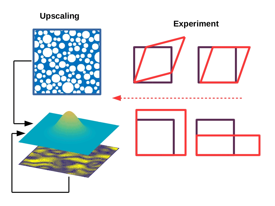
Figure 1: Experimental setup

5.1.1 Validation

To validate our method, we compare Bayesian upscaling procedure to the deterministic homogenisation approach as presented in [44]. Therefore, we initally observe only one realisation of the random mesostructure and apply periodic boundary conditions. An example of the fine scale response in terms of stored energy function is shown in Fig. 2 for Exp 1.

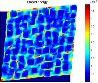
Figure 2: Fine scale response under shearing with periodic boundary conditions

As depicted in Fig. 3, the deterministic homogenisation (DHB) fails to predict the shear moduli in purely compression state (Exp 4). Similar holds for the bulk moduli in case when only shear loading conditions are applied (Exp 1). The reason is that in the absence of measurement information on one of the material characteristics, the deterministic homogenisation becomes ill-posed. On the other hand, the Bayesian updating approach (BUB) in a form of Eq. (53) regularises the problem by introducing the prior information. This means that the posterior estimate matches the prior when the data are not informative about the parameter set. Otherwise, the posterior mode and the deterministic homogenised value are identical. To conclude, the Bayesian upscaling procedure is more robust than the classical one. In addition, one may show that the Bayesian upscaling procedure is more appropriate as one may sequentially introduce the measurement data into the upscaling process. For example, one may first use the measurement information coming from the fourth experiment to obtain the upscaled material properties. These further can be used as a new prior for the third experiment, and so on, see 3.

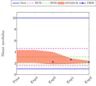
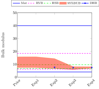
RVB$=$Reuss-Voight bounds, HSB$=$Hashin-Strikman bounds, BUB$=$Bayesian updating bounds, DHB$=$classical homogenisation

Figure 3: Upscaling of deterministic material properties: a) shear mnoduli b) bulk moduli

5.1.2 Upscaling of random elastic material

To quantify randomness on the meso-scale level, the previously described experiment is repeated several times, and the avaraged stored elastic energies per experiment are collected. In particular, we observe realisations of the meso-scale elastic material described by randomly placed inclusions depicting the volume fraction of 40%. Initially, the stored energy is identified given observed data by using the variational Bayesian inference method as described in Section 4. The logarithm of energy is modelled by a copula Gaussian mixture model, and the individual components are identified. The optimal number of mixture components is further decoupled by inverse transform. The resulting uncorrelated random variables are then further used to obtain the polynomial chaos surrogate of the measurement data.

The fine-scale simulation is performed on the 2D micro-structure with increasing number of particles and linear displacement based boundary condition. The material properties of the matrix phase are taken to be: the bulk moduli is $K_{m}=4$ and shear moduli is $G_{m}=1$, whereas the inclusions characteristics are prescribed to be ten times higher. For a given number of particles embedded in the matrix phase, an ensemble of 100 realizations of stored energy is considered to gather corresponding measurement set. In Fig. 4 the PDFs for the identified elastic energies are shown for pure shear and bi-axial compression test, respectively. As expected, the variation of stored energy reduces with the increase of the number of particles in the matrix phase. However, it is interesting to note that in compression case the mean responses of stored energies vary more than in a pure shear test. This is closely related to the way how boundary conditions are imposed. Namely, we take into consideration directly the element on which the loadings are imposed, and thus one may recognise the strong influence of boundary conditions on the obtained results. In a more proper analysis one would take into consideration only internal element, which is away from the boundary as shown in Fig. 5.

In case of 64 embedded particles, the mean meso-scale energy tends to converge as one increases the size of Monte Carlo ensemble set. This is in contrast with its 4 particle counterpart, the energy of which keeps on fluctuating, see Fig. 6a). This behaviour is more pronounced in Fig. 6b), which depicts the dependence of the $p_{50}$, $p_{75}$, $p_{95}$ and $p_{99}$ quantiles on the number of embbeded particles in a matrix phase. The mean energy tends to stabilize to a fixed value, whereas the corresponding bounds tend to shrink towards the mean value when the number of particles increases. Hence, the uncertainty becomes less pronounced.

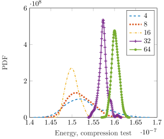
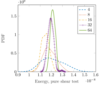
Figure 4: Measured energy on 100 mesostructure realisations for different number of inclusions and random position only. The boundary condition is linear displacement.

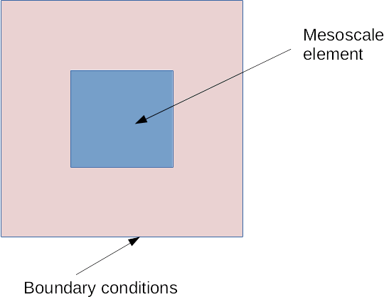
Figure 5: Element definition for the upscaling procedure

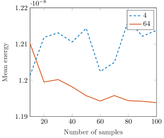
Figure 6: Measured energy on 100 mesostructure realisations for different number of inclusions and random position only. The boundary condition is linear displacement. Left: the mean convergence w.r.t. number of Monte Carlo samples, right: Quantiles of energy w.r.t. number of particles.

The previously discussed results are conditional estimates of stored energy given its samples. These consist of two kinds of uncertainties: aleatoric (meso-scale randomness) and epistemic (prior information). Estimating the confidence intervals w.r.t. to the epistemic uncertainties one obtains the corresponding PDFs of upscaled material properties: the mean PDF which represents purely aleatory uncertainty and $p_{95}$ upper and lower PDF’s that describe $95\%$ quantiles on the mean PDF, see Fig. 7. The result indicates that the PDF in case of 4 particles is slightly underestimated, whereas the PDF in case of 64 particles is overestimated. This phenomenon is often observed when variational inference is used instead of full Bayes’s rule. Naturaly the quantile intervals strongly depend on the size of the measurement set. In Fig. 8 one may notice that with the smaller measurement set (e.g. 10 samples) our confidence about the upscaled PDF is lower than in case of higher number of measurements (e.g. 80 samples).

Figure 7: Confidence bounds of estimate a) 4 particles b) 64 particles for the compression experiment

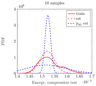
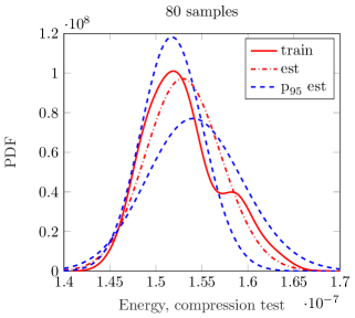
Figure 8: Dependence of confidence bounds on the number of samples used in estimation. THe number of particles is 4. The loading is compression

Besides previous analysis, the impact of boundary conditions on the upscaled quantities is another important factor to study. In Fig. 9 and Fig. 10 are depicted $50\%$ and $95\%$ quantiles of energy for linear discplacement (LD), periodic (PR) and unifrom tension (UT) boundary conditions. According to these results, linear displacement defines the upper bound on the estimated energy, whereas uniform tension gives its lower limit. On the other hand, variations of energies are similar for all three types of boundary conditions, and are inverse proportional to the number of inclusions.

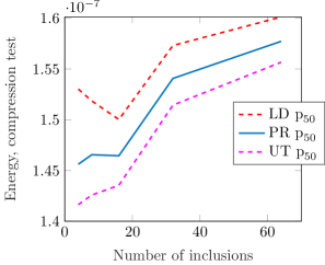
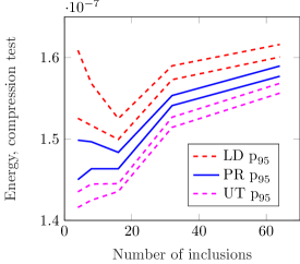
Figure 9: Energy wrt boundary conditions and number of inclusions

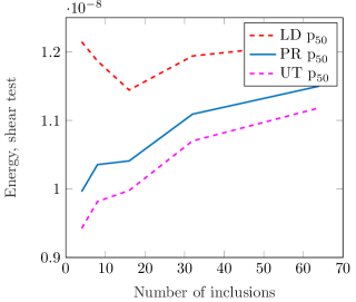
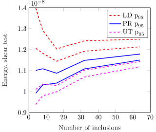
Figure 10: Energy wrt boundary conditions and number of inclusions

Once the measurement energy is identified, in the second step we use the proxy of $y_{m}$ to identify the elastic macro-scale material characteristics by using the generalised Kalman filter given in Eq. (53). When using this type of upscaling one is biased to prior knowledge on the material characteristics on the coarse scale. In a multiscale analysis, however, it is not an easy task to define the prior knowledge, or better to say the limits of the prior distribution. Therefore, in Fig. 11 is investigated the posterior change of shear moduli w.r.t. prior knowledge. The prior distributons are chosen such that $95\%$ limits match interval described by material property of the matrix phase and inclusion (in figure denoted by MAT), Reuss-Voigt (RV) or Hashin-Shtrikman (HS) bounds. Their corresponding $95\%$ posterior limits are depicted in Fig. 11a). Interesting to note is that even though the posterior of the upscaled shear moduli changes w.r.t. prior assumption, its mean remains the same, see Fig. 11b). Therefore, there is only one mean PDF in the plot. To better understand this point, the shear moduli update is obtained by using the linear Kalman formula

$$\mu_{a}(\zeta,\theta)=\mu_{f}(\theta)+K(y_{m}(\zeta)-y_{M}(\theta))$$ (85)

in which $K$ denotes the Kalman gain. Hence, in Fig. 11a are shown $95\%$ bounds of total posterior $\mu_{a}(\zeta,\theta)$, whereas in Fig. 11b are depicted $95\%$ bounds of $\mathbb{E}_{\theta}(\mu_{a}(\zeta,\theta))$ and hence only aleatory uncertainty. Therefore, all estimates match. Similar holds for the bulk moduli, see Fig. 12.

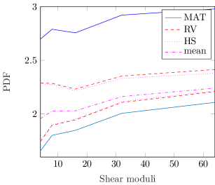
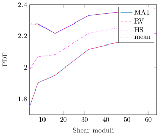
Figure 11: Estimated shear moduli w.r.t. prior choice

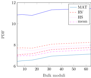
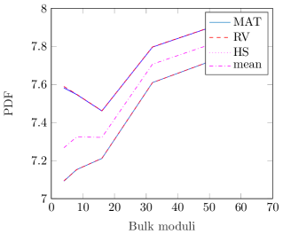
Figure 12: Estimated bulk moduli w.r.t. prior choice

To validate our result, further in Fig. 13 we compare the mean posterior distribution $\mathbb{E}_{\theta}(\mu_{a}(\zeta,\theta))$ with the posterior distribution obtained by repeating the deterministic homogenisation, see [44], on each of the meso-scale realisations. As one may notice, the distributon coming from the deterministic homogenisation and the one obtained by our approach are matching. They are further compared with the posterior distribution represented by $\mu_{a}(\zeta,\theta)$, i.e. the total uncertainty that includes both aleatory and epistemic knowledge.

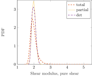
Figure 13: Estimated shear moduli: total: $\mu_{a}(\zeta,\theta)$, partial: $\mathbb{E}_{\theta}(\mu_{a})$, det: deterministic homogenisation

So far the fine-scale randomness has been considered for the positioning of particles in the matrix phase. In the ensuing discussion, next to the random position the uncertainty associated with the material properties is also considered. For the numerical experiment bi-axial compression or pure shear periodic boundary conditions are chosen. The number of particles in the sample are 64 constituting $40\%$ of the total volume. In Fig. 14 is depicted change in the energy PDF, equipped with randomness in: only position (pos) and both position and material (pos+mat), respectively. To material properties on fine scale are assigned lognormal distributions with the same mean as in the previous experiment and $10\%$ of the variation. As one would suspect, the PDF for the random position and material case has bigger spread than the one for only random position. Similar behaviour is observed in the PDF of the upscaled bulk modulus - as shown in Fig. 15. This spread is also observed when using different types of boundary conditions as shown in Fig. 17 in which the left figure stands for the total uncertainty upper $95\%$ limits (aleatory+epistemic), whereas the right figure stands for the $95\%$ limits of aleatory randomness only. Similar is depicted for the shear moduli in Fig. 16.

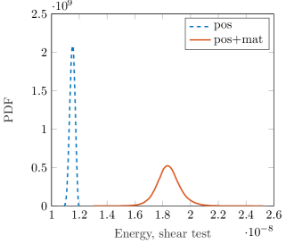
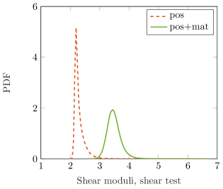
Figure 14: Estimated shear energy and shear moduli w.r.t. randomness in position and material properties on the mesoscale

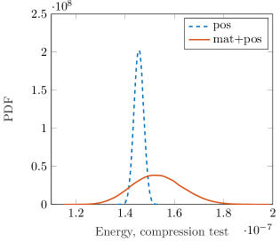
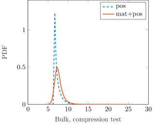
Figure 15: Estimated compression energy and bulk moduli w.r.t. randomness in position and material properties on the mesoscale

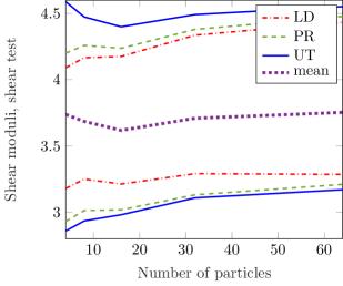
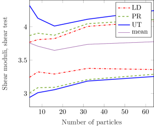
Figure 16: Estimated upper and lower 95% quantiles of shear moduli w.r.t. type of boundary condition. Left is the total a posteriori uncertainty (aleatory+epistemic), whereas right is only aleatory one.

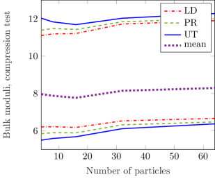
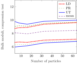
Figure 17: Estimated upper and lower 95% quantiles of bulk moduli w.r.t. type of boundary condition. Left is the total a posteriori uncertainty (aleatory+epistemic), whereas right is only aleatory one.

5.2 Upscaling of damage pheonmena

In this subsection, the proposed approach is applied to another interesting problem. For this purpose a phenomenological elasto-damage model is considered as described in the beginning of this section. The goal is to compute a homogenized description of random material parameters on coarse-scale given fine-scale measurements. Fine-scale is assumed to follow same constitutive model as coarse-scale, however the material parameters are being random. For validation purpose they are also assumed to be homogeneous, and then in the second case scenario also spatially varying. In both experiments we only simulate the displacement controlled biaxial compression of 2D block with unit length ( similar to the experiment in the previous example). The deformation tensor - applied to the boundary nodes of the specimen - is specified as:

$$\mathcal{F}=\begin{bmatrix}-p&0\\ 0&-p\end{bmatrix}$$ (86)

where $p$ is the propotional factor for applied displacement, which varies with time increments $t_{i}$ according to the values in set $(t_{i},p_{i}):\{(0,0),(3,0.00025),(10,0.00035)\}$

5.2.1 Validation

For validation purposes the material parameters $\kappa_{m}(\omega_{\kappa})$ on the fine-scale are modelled as lognormal random variables with the mean $\mu_{\kappa}:=\{2.0444,0.92,0.0031,0.0047)\cdot 10^{11}$ and the coefficient of correlation $5\%$. After propagating the variables through the elaso-damage model, the corresponding elastic, damage and hardening energies are estimated. We assume that the polynomial chaos approximation of the energy measurement is not given, but only a set of 100 samples. Therefore, the log of energies are modelled as copula Gaussian mixtures with the unknown number of components. The simulation is run in 8 equidistant time steps, the first two being elastic. In the third to sixth steps the behaviour is combination of elasticity and damage, whereas in the last step is predominated by the damage component. In Fig. 18 are shown scatter plots of energies in the first and the third step, both depicting two states in the response: elastic and damage. The linear components are linearly related as expected, whereas the correlation between the damage and the elastic step is random. To uncouple the measurement data, we observe energies at the last time step (full damage state) as depicted in Fig. 19. Clearly, the hardening and damage energies are almost linearly related in the log-space, whereas this doesnt hold for the damage and elastic part of energy. Both copula and inividual components are estimated as discussed in Section 4. In order to decouple the complete set, the inverse transform is applied in order to obtain uncorrelated Gaussian samples. These are further used to generate the polynomial chaos expansions for all time steps by Bayes’s rule as presented in Section 3. In this manner one may obtain prediction of energies at the meso-scale for all time steps. These are further adoped as approximation of the measurement $y_{m}$. Furthermore, one assumes that the material parameters used for prediction of coarse-scale simulation are not known, and are assumed to be uncertain. Due to positive definitness requirement they are also modelled as lognromal random variables with the mean $20\%$ bigger than in the fine-scale case and coefficient of correlation $20\%$. The resulting updated coarse-scale properties are shown in Fig. 21. The bulk moduli and the limit stress that initiates the damage are both updated and match the true distribution, whereas their correlation and the mapping to the normal space is shown in Fig. 20. On the other hand, due to chosen experiment both shear and hardening moduli stay unindentified as they are not observable.

In the previously described experiment the relationships between the measurement data and their approximations are too complex in order to be properly modelled. Therefore, the experiment is repeated in same setting, only this time the measurement is not functionally aproximated. Instead, the inverse problem is solved for each individual sample of measurement (each RVE), and then the updated parameters are collected into the set of parameter samples. This calculation is expected to be simpler than the previous one as the relationships between the material parameters are easier to model. By collecting mean value of posterior distributions, one may model the set of parameters as copula Gaussian mixture similarly to the previous case. After mapping to the Gaussian space the corresponding coarse-scale estimates can be functionally approximated by a polynomial chaos expanion obtained by Bayes’ rule. In Fig. 22 is depicted the difference between this approach (est1) and the previous one (est2), as well as joint distribution between the bulk moduli and $\sigma_{f}$.

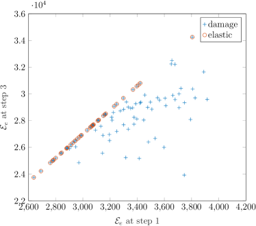
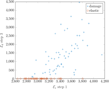
Figure 18: Dependence of elastic ($\mathcal{E}_{e}$) and dissipative ($\mathcal{E}_{d}$) energies between the linear elastic step 1 and nonlinear step 3

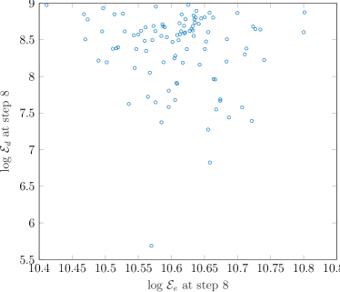
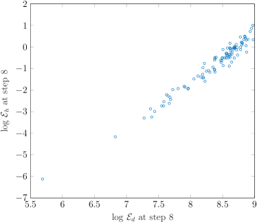
Figure 19: Dependence of elastic ($\mathcal{E}_{e}$) and dissipative ($\mathcal{E}_{d}$) energies between at the full damage step 8

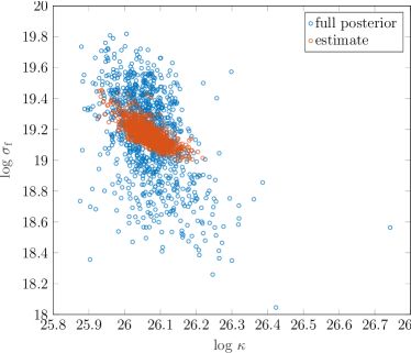
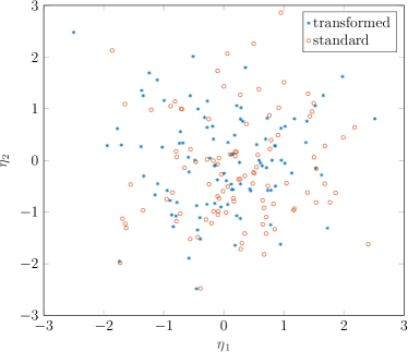
Figure 20: Left: The relationship between the macro-scale estimated properties w.r.t. to full posterior measure (aleatory+epistemic uncertainty) and its epistemic mean (only aleatory uncertainty). Right: Comparison of 100 samples of mapped Gaussian random variables from the estimated macro-parameters and independent standard Gaussians.

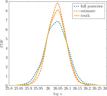
Figure 21: Estimated posterior macroparameters w.r.t. to their true value. Full posterior represents both aleatory and epistemic uncertainty, whereas estimate is only aleaotry one.

Figure 22: Left: comparison of two upscaling strategies, right: correlation between the macro-scale parameters.

5.2.2 Upscaling of heterogeneous medium

The model is implemented in a finite element framework ( see [19, 26] for more details) and is used to demonstrate the proposed up-scaling strategy. For this purpose, a 2D square block of unit length is considered. To emulate the coarse and fine-scale descriptions in the finite element setting, the 2D block is considered as one element on the coarse-scale, whereas the fine-scale comprises of 2500 elements. The block is deformed by discplacement controlled bi-axial compression as shown in Fig. 23.

Figure 23: The deformation of the 2d block by bi-axial compression

As far as material description is concerned, the material properties on the heterogeneous fine-scale are a priori assumed to be realizations of log-normal random fields with the statistics depicted in Table 1, and Gaussian covariance functions. These are simulated using different values of correlation length $l_{c}\in\{5l_{e},10l_{e},25l_{e}\}$ ($l_{e}$ is the element length on the fine-scale) and coefficients of variation $c_{var}\in\{5\%,10\%\}$. In Fig. 25 is shown an example of the meso-scale random field realisations given different correlation lengths. The realisation is becoming smoother when the correlation length increases. This means that the material becomes homogeneous in the limit $\ell_{c}=\infty$. On the other hand, the coarse-scale material properties are taken a priori as a lognormal random variables, with the same mean and standard deviation as their meso-scale counterpart.

The measurement data are made of three type of avaraged energies: the stored elastic energy $\mathcal{E}_{e}$ (see Eq. (80)), the damage dissipation $\mathcal{E}_{d}$ (i.e. the first term in Eq. (80) ), and the hardening part $\mathcal{E}_{h}$ of the dissipation energy (i.e. the second term in Eq. (80)). Their logarithms are simulated using mixture models and vine copulas, and further identified using variational Bayes rule. Similarly to the experiment in the validation section, in the first two simulation steps one may observe only elastic energy as the dissipation effects do not appear. Therefore, we start the simulation with the last step, and approximate the corresponding energies by mixture models and vine copulas, see Fig. 24. The complete simulation steps from the previous section are repeated.

As shown in Fig. 26 the variation of energies increases with the correlation length size for the case when the $c_{var}$ of the meso-scale random field is taken to be $10\%$. The reason for this is that energy realisations are less fluctuating with increasing correlation length, but their avarage value is more pronaunced as prospective fluctuations do not cancel out, as similar can be concluded when observing Fig. 25 on the left hand side. This holds for all energy estimates, and can be explained by Fig. (27) in which the presence of damage on one of the responses is shown. With increase of the correlation length the damage is more pronaunced and hence one expected higher variations. In addition, one may also conclude that the corresponding PDFs are becoming more skewed when the material model approaches homogeneous case. The skewness in terms of long tailes is not completely caused by variations of the random meso-scale, but also by inaccuracy of the variational method used for the PCE estimation of the measurement due to overestimation.

On the right side of Fig. 26 one may observe the energy evolution w.r.t. to time. Here, $c_{var}$ of the corresponding meso-scale random field is chosen to be $10\%$ and the correlation length is $\ell_{c}=10\ell_{e}$ . The top figure depicts the elastic energy. As expected, the energy variation grows in time. On the contrary, the damage energy seen in the middle does not alter much the PDF form. The damage initialises in the thrid step, and mostly shifts towards higher average value due to increased presence of damage as shown in Fig. 28. Finally, the hardening energy increases, but also changes the PDF form significantly in time.

The up-scaled parameter estimates behave similarly to the energy estimates as shown in Fig. 29. The hardening parameter doesnt get updated, and stays constant over time. Similar holds for the correlation length as the hardening energy doesnt change with the correlation length.

Property	$\kappa$	$\sigma_{f}$	$K_{d}$
$\mu$	204440	300	450
$\sigma$	10222	15	22.5

Table 1: Fine-scale statistics for elasto-damage constitutive model (in MPa)

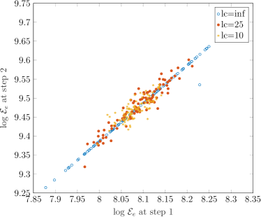
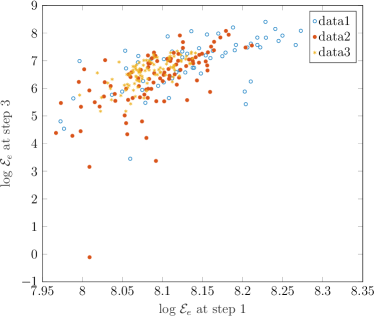
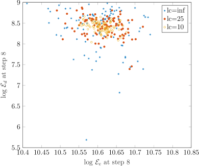
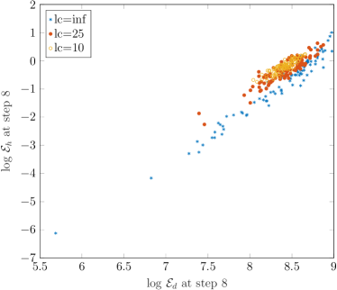
Figure 24: Energies dependence w.r.t to different time steps

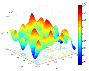
(a) $\ell_{c}=5\ell_{e},c_{var}=5\%$

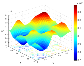
(b) $\ell_{c}=10\ell_{e},c_{var}=5\%$

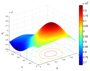
(c) $\ell_{c}=25\ell_{e},c_{var}=5\%$

Figure 25: The damage stress realisations using different values of the correlation length $\ell_{c}$

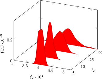
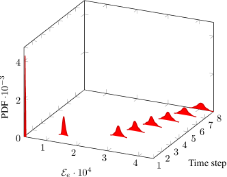
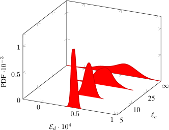
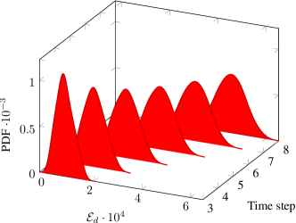
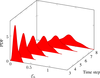
Figure 26: The energy PDF w.r.t. the correlation length (left) $\ell_{c}$ and time steps (right)

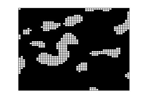
Figure 27: The presence of damage on the meso-scale for $c_{var}=0.1$ and $\ell_{c}=5\ell_{e}$, $\ell_{c}=10\ell_{e}$, $\ell_{c}=25\ell_{e}$

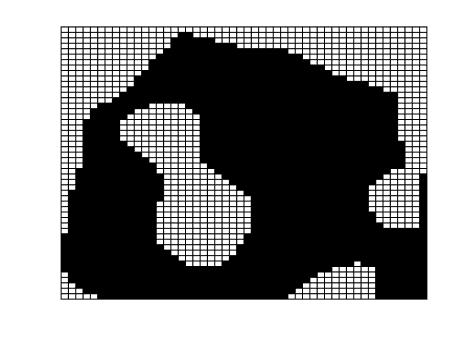
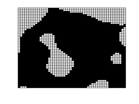
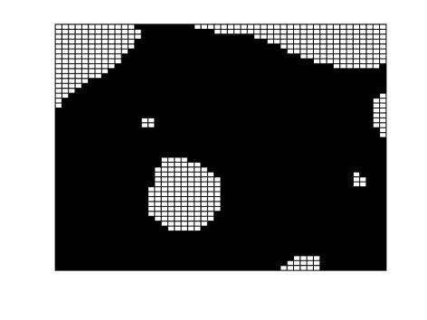
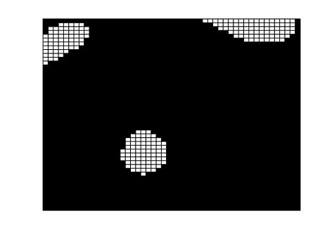
Figure 28: The presence of damage on the meso-scale w.r.t. time step for $c_{var}=0.1$ and $\ell_{c}=10\ell_{e}$

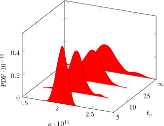
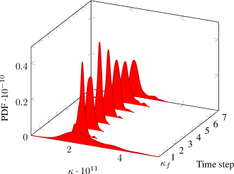
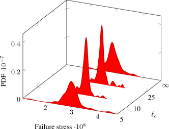
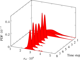
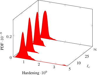
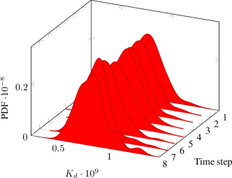
Figure 29: The PDF of parameters $\kappa$, Failure stress $\sigma_{d}$ and Hardening modulus $K_{d}$ w.r.t. the correlation length (left) $\ell_{c}$ and time steps (right)

6 Conclusion

The stochastic multiscale analysis as previously presented is one praticular kind of inverse problem in which the coarse-scale parameters are to be estimated given the fine-scale information. In this paper we employed the energy conservation principle in order to estimate the macro-scale parameters given meso-scale energy descriptions. Such an approach is then allowing derivation of new constitutive laws on the macroscale counterpart, the ones that are optimally matching the energy information. Furthermore, we show that in a case when the fine scale energy information is of deterministic kind, i.e. describes the particular RVE, the process of estimation can be easily done by employing the nonlinear version of the Kalman filter. The filter then represents the map between the observation and the quantity of interest, i.e. the macro-scale model parameters, or the model itself. In addition, we have shown that this kind of mapping can be also used in a more general situation in which the fine scale information is described by uncertainty. The only requirement to achieve this is to fully specify the random variable representing the data, i.e. to describe its probability distribution. For this purpose we employ the Bayes variational inference in combination with the copula theory. Computationally, the measurement probability distribution is then represented by a functional approximation in terms of the polynomial chaos expansion obtained by mapping the measurement data to the Gaussian space, applying an inverse transform and using an additional sparse Bayes variational inference for the purpose of estimation of the expansion coefficients. As the inervse map from the energy space to the Gaussian one is not easy to approximate, we recommend to first discretise the energy space (i.e. sample), and then to map each sample to the macroscale model parameters. As shown on both linear elastic and elasto-damage examples, the latter ones can be more accurate approximated. Note that in this paper we have only observed the elasto-damage models on two scales under one specific loading condition. However, in practice this will not suffice to achieve good macro-scale representation. Therefore, the next step to be considered is to add different loading conditions into estimation.

References

- [1] Le Ba Anh, Julien Yvonnet, and Q.‐C He. Computational homogenization of nonlinear elastic materials using neural networks: Neural networks-based computational homogenization. International Journal for Numerical Methods in Engineering, 104, 05 2015.
- [2] A. Banerjee, X. Guo, and H. Wang. On the optimality of conditional expectation as a bregman predictor. IEEE Trans. Information Theory, 51(7):2664–2669, 2005.
- [3] Christopher M. Bishop. Pattern Recognition and Machine Learning (Information Science and Statistics). Springer-Verlag, Berlin, Heidelberg, 2006.
- [4] Christopher M. Bishop and Michael E. Tipping. Variational relevance vector machines. CoRR, abs/1301.3838, 2013.
- [5] Lukas Bruder and Phaedon-Stelios Koutsourelakis. Beyond black-boxes in bayesian inverse problems and model validation: applications in solid mechanics of elastography. arXiv preprint arXiv:1803.00930, 2018.
- [6] A Clément, Christian Soize, and Julien Yvonnet. Computational nonlinear stochastic homogenization using a nonconcurrent multiscale approach for hyperelastic heterogeneous microstructures analysis. International Journal for Numerical Methods in Engineering, 91(8):799–824, 2012.
- [7] A Clément, Christian Soize, and Julien Yvonnet. High-dimension polynomial chaos expansions of effective constitutive equations for hyperelastic heterogeneous random microstructures. In Congress on Computational Methods in Applied Sciences and Engineering (ECCOMAS 2012), pages 1–2. Vienna University of Technology, Vienna, 2012.
- [8] Alexandre Clément, Christian Soize, and Julien Yvonnet. Uncertainty quantification in computational stochastic multiscale analysis of nonlinear elastic materials. Computer Methods in Applied Mechanics and Engineering, 254:61–82, 2013.
- [9] P. Emberchts B. Sudret E. Torre, S. Marelli. A general framework for data-driven uncertainty quantification under complex input dependencies using vine copulas. Probabilistic Engineering Mechanics, 55:1, 2019.
- [10] L Felsberger and PS Koutsourelakis. Physics-constrained, data-driven discovery of coarse-grained dynamics. arXiv preprint arXiv:1802.03824, 2018.
- [11] Frederic Feyel. A multilevel finite element method (fe2) to describe the response of highly non-linear structures using generalized continua. Computer Methods in Applied Mechanics and Engineering, 192:3233–3244, 07 2003.
- [12] Frédéric Feyel and Jean-Louis Chaboche. Fe2 multiscale approach for modelling the elastoviscoplastic behaviour of long fibre sic/ti composite materials. Computer Methods in Applied Mechanics and Engineering, 183(3):309 – 330, 2000.
- [13] Isabell M Franck and Phaedon-Stelios Koutsourelakis. Multimodal, high-dimensional, model-based, bayesian inverse problems with applications in biomechanics. Journal of Computational Physics, 329:91–125, 2017.
- [14] Isabell M Franck and PS Koutsourelakis. Sparse variational bayesian approximations for nonlinear inverse problems: Applications in nonlinear elastography. Computer Methods in Applied Mechanics and Engineering, 299:215–244, 2016.
- [15] Isabell M Franck and PS Koutsourelakis. Constitutive model error and uncertainty quantification. PAMM, 17(1):865–868, 2017.
- [16] Marc GD Geers, Varvara G Kouznetsova, Karel Matouš, and Julien Yvonnet. Homogenization methods and multiscale modeling: Nonlinear problems. Encyclopedia of Computational Mechanics Second Edition, pages 1–34, 2017.
- [17] R. Ghanem and P. D. Spanos. Stochastic finite elements—A spectral approach. Springer-Verlag, New York, 1991.
- [18] Lori Graham-Brady. Statistical characterization of meso-scale uniaxial compressive strength in brittle materials with randomly occurring flaws. International Journal of Solids and Structures, 47(18):2398 – 2413, 2010.
- [19] A. Ibrahimbegovic. Nonlinear Solid Mechanics: theoretical formulations and finite element solution methods. Springer Netherlands, Netherlands, 2006.
- [20] A. Frigessi H. Bakken K. Aas, C. Czado. Pair-copula construction of multiple dependence. Insurance Mathematics and Economics, 44:182, 2009.
- [21] Phaedon-Stelios Koutsourelakis. Stochastic upscaling in solid mechanics: An excercise in machine learning. Journal of Computational Physics, 226(1):301–325, 2007.
- [22] Phaedon-Stelios Koutsourelakis. Variational bayesian strategies for high-dimensional, stochastic design problems. Journal of Computational Physics, 308:124–152, 2016.
- [23] Junwei Liu and Lori Graham-Brady. Perturbation-based surrogate models for dynamic failure of brittle materials in a multiscale and probabilistic context. International Journal for Multiscale Computational Engineering, 14(3):273–290, 2016.
- [24] Xiaoxin Lu, Dimitris G. Giovanis, Julien Yvonnet, Vissarion Papadopoulos, Fabrice Detrez, and Jinbo Bai. A data-driven computational homogenization method based on neural networks for the nonlinear anisotropic electrical response of graphene/polymer nanocomposites. Computational Mechanics, 64(2):307–321, Aug 2019.
- [25] C. Wang M. D. Hoffman, D. M. Blei and J. Pasley. Stochastic variational inference. Journal of Machine Learning Research, 14:1303–1347, 2013.
- [26] H. G. Matthies M. S. Sarfaraz, B. Rosić and A. Ibrahimbegović. Stochastic upscaling via linear bayesian updating. Coupled systems mechanics, 7(2):211–231, 2018.
- [27] Juan Ma, S Sahraee, Peter Wriggers, and Laura De Lorenzis. Stochastic multiscale homogenization analysis of heterogeneous materials under finite deformations with full uncertainty in the microstructure. Computational Mechanics, 55:819–835, 05 2015.
- [28] Juan Ma, S Sahraee, Peter Wriggers, and Laura De Lorenzis. Stochastic multiscale homogenization analysis of heterogeneous materials under finite deformations with full uncertainty in the microstructure. Computational Mechanics, 55:819–835, 05 2015.
- [29] Juan Ma, Ilker Temizer, and Peter Wriggers. Random homogenization analysis in linear elasticity based on analytical bounds and estimates. International Journal of Solids and Structures, 48:280–291, 01 2011.
- [30] Juan Ma, Peter Wriggers, and Liangjie Li. Homogenized thermal properties of 3d composites with full uncertainty in the microstructure. Structural Engineering and Mechanics, 57:369–387, 01 2016.
- [31] Juan Ma, Suqin Zhang, Peter Wriggers, Wei Gao, and Laura De Lorenzis. Stochastic homogenized effective properties of three-dimensional composite material with full randomness and correlation in the microstructure. Computers and Structures, 144:62–74, 11 2014.
- [32] H. G. Matthies, E. Zander, B. Rosić, and A. Litvinenko. Parameter estimation via conditional expectation: a Bayesian inversion. Advanced Modeling and Simulation in Engineering Sciences, 3(1):1–21, 2016.
- [33] A. Mielke and T. Roubicek. Rate independent systems: Theory and application. Springer, New York, 2015.
- [34] Bojana Rosic. Stochastic state estimation via incremental iterative sparse polynomial chaos based bayesian-gauss-newton-markov-kalman filter, 2019.
- [35] K. Sagiyama and K. Garikipati. Machine learning materials physics: Deep neural networks trained on elastic free energy data from martensitic microstructures predict homogenized stress fields with high accuracy. arXiv e-prints, page arXiv:1901.00524, Jan 2019.
- [36] Dimitrios Savvas and George Stefanou. Determination of random material properties of graphene sheets with different types of defects. Composites Part B: Engineering, 143:47 – 54, 2018.
- [37] Dimitrios Savvas, George Stefanou, and Manolis Papadrakakis. Determination of rve size for random composites with local volume fraction variation. Computer Methods in Applied Mechanics and Engineering, 305:340 – 358, 2016.
- [38] Markus Schöberl, Nicholas Zabaras, and Phaedon-Stelios Koutsourelakis. Predictive collective variable discovery with deep bayesian models. arXiv preprint arXiv:1809.06913, 2018.
- [39] A Sklar. Fonctions de répartition à n dimensions et leurs marges. Publications de l’Institut Statistique de l’Université de Paris, 8:229–231, 1959.
- [40] B. Staber and J. Guilleminot. Functional approximation and projection of stored energy functions in computational homogenization of hyperelastic materials: A probabilistic perspective. Computer Methods in Applied Mechanics and Engineering, 313:1 – 27, 2017.
- [41] George Stefanou. Simulation of heterogeneous two-phase media using random fields and level sets. Frontiers of Structural and Civil Engineering, 9(2):114–120, Jun 2015.
- [42] George Stefanou, Dimitrios Savvas, and Manolis Papadrakakis. Stochastic finite element analysis of composite structures based on material microstructure. Composite Structures, 132:384 – 392, 2015.
- [43] George Stefanou, Dimitrios Savvas, and Manolis Papadrakakis. Stochastic finite element analysis of composite structures based on mesoscale random fields of material properties. Computer Methods in Applied Mechanics and Engineering, 326:319 – 337, 2017.
- [44] Ilker Temizer. Micromechanics: analysis of heterogeneous materials, 2012.
- [45] Dustin Tran, David M. Blei, and Edoardo M. Airoldi. Copula variational inference. In NIPS, 2015.
- [46] Viet Hung Tran. Copula variational bayes inference via information geometry. CoRR, abs/1803.10998, 2018.
- [47] Jörg Unger and Carsten Könke. An inverse parameter identification procedure assessing the quality of the estimates using bayesian neural networks. Appl. Soft Comput., 11:3357–3367, 06 2011.
- [48] Jörg F. Unger and Carsten Könke. Coupling of scales in a multiscale simulation using neural networks. Computers & Structures, 86(21):1994 – 2003, 2008.
- [49] N. Wiener. The homogeneous chaos. American Journal of Mathematics, 60:897–936, 1938.
- [50] Dongbin Xiu. Numerical Methods for Stochastic Computations: A Spectral Method Approach. Princeton University Press, Princeton, NJ, USA, 2010.