Abstract

Time-varying parameter (TVP) models are very flexible in capturing gradual changes in the effect of a predictor on the outcome variable. However, in particular when the number of predictors is large, there is a known risk of overfitting and poor predictive performance, since the effect of some predictors is constant over time. We propose a prior for variance shrinkage in TVP models, called triple gamma. The triple gamma prior encompasses a number of priors that have been suggested previously, such as the Bayesian lasso, the double gamma prior and the Horseshoe prior. We present the desirable properties of such prior and its relationship to Bayesian Model Averaging for variance selection. The features of the triple gamma prior are then illustrated in the context of time varying parameter vector autoregressive models, both for simulated dataset and for a series of macroeconomics variables in the Euro Area.

xx 1 5 Received: date; Accepted: date; Published: date Triple the gamma – A unifying shrinkage prior for variance and variable selection in sparse state space and TVP models Annalisa Cadonna ¹, Sylvia Frühwirth-Schnatter ^1,∗ and Peter Knaus ¹ Annalisa Cadonna, Sylvia Frühwirth-Schnatter and Peter Knaus Correspondence: sfruehwi@wu.ac.at

1 Introduction

Model selection in a high-dimensional setting is a common challenge in statistical and econometric inference. The introduction of Bayesian model averaging (BMA) techniques in the statistical literature (Raftery et al., 1997; Brown et al., 2002; Cottet et al., 2008) has led to many interesting applications, see, among others, (Koop and Potter, 2004; Sala-i-Martin et al., 2004; Kleijn and van Dijk, 2006; Frühwirth-Schnatter and Tüchler, 2008) for early references in econometrics.

Predictor selection for possibly very high-dimensional regression problems though shrinkage priors is an attractive alternative to BMA which relies on discrete mixture priors, see Bhadra et al. (2019) for an excellent review. There is a vast and growing literature on shrinkage priors for regression problems that focuses on the following aspects. First, how to choose sensible priors for high-dimensional model selection problems in a Bayesian framework, second, how to design efficient algorithms to cope with the associated computational challenges and third, to investigate, both from a theoretical and a practical viewpoint, how such priors perform in high-dimensional problems.

A striking duality exists in this very active area between Bayesian and traditional approaches. For many shrinkage priors, the mode of the posterior distribution obtained in a Bayesian analysis can be regarded as a point estimate from a regularization approach, see Fahrmeir et al. (2010) and Polson and Scott (2012). One such example is the popular Lasso (Tibshirani, 1996) which is equivalent to a double-exponential shrinkage prior in a Bayesian context (Park and Casella, 2008). However, the two approaches differ when it comes to selecting penalty parameters that impact the sparsity of the solution. One advantage of the Bayesian framework in this context is that the penalty parameters are considered to be unknown hyperparameters which can be learned from the data. Such “global-local” shrinkage priors (Polson and Scott, 2011) adjust to the overall degree of sparsity that is required in a specific application through a global shrinkage parameter and separates signal from noise through local, individual shrinkage parameters.

While predictor selection though shrinkage priors in regression models is addressed in a vast literature, the use of shrinkage priors for more general econometric models for time series analysis, such as state space models and time-varying parameter (TVP) models is, in comparison, less well-studied. Sparsity in the context of such models refers to the presence of a few large variances among many (nearly) zero variances in the latent state processes that drive the observed time series data. A common goal in this setting is to recover a few dynamic states, driven by such a state space model, among many (nearly) constant coefficients. As shown by Frühwirth-Schnatter and Wagner (2010), this variance selection problem can be cast into a variable selection problem in the non-centered parametrization of a state space model. Once this link has been established, shrinkage priors that are known to perform well in high-dimensional regression problems can be applied to variance selection in state space models, as demonstrated for the Lasso (Belmonte et al., 2014) and the normal-gamma (Griffin and Brown, 2017; Bitto and Frühwirth-Schnatter, 2019).

Despite this already existing variety, we introduce a new shrinkage prior for variance selection in sparse state space and TVP models in the present paper, called triple gamma prior as it has a representation involving three gamma distributions. This prior can be related to various shrinkage priors that were found to be useful for high-dimensional regression problems such as the generalized beta mixture prior (Armagan et al., 2011) and contains the popular Horseshoe prior (Carvalho et al., 2009, 2010) as a special case. Furthermore, the half-$t$ and the half Cauchy (Gelman, 2006; Polson and Scott, 2012), suggested as robust alternatives to the inverse gamma distribution for variance parameters in hierarchical models, as well as the Lasso and the double gamma, are special cases of the triple gamma. In this context, the triple gamma can also be regarded as an extension of the scaled beta2 distribution (Pérez et al., 2017).

Among Bayesian shrinkage priors, usually a clear distinction is made between two-group mixture or spike-and-slab priors and continuous shrinkage priors, of which the triple gamma is a special case. An important contribution of the present paper is to show that the triple gamma provides a bridge between these two approaches and has the following property which is favourable both in sparse and dense situations. One of the hyperparameters allows high concentration over the region in the shrinkage profile that is relevant for shrinking noise, while the other hyperparameter allows high concentration over the region that prevents overshrinking of signals. This leads to a behaviour of the triple gamma prior that very much resembles Bayesian model averaging based on discrete spike-and-slab priors, with a strong prior concentration at the corner solutions where some of the variances are nearly close to zero. While this is reminiscent of the Horseshoe prior, the shrinkage profile induced by the triple gamma is more flexible than that of a Horseshoe. Thanks to the estimation of the hyperparemters, it is not constrained to be symmetric around one half, enabling adaption to varying degrees of sparsity in the data.

The triple gamma prior also scores well from a computational perspective. While exploring the full posterior distribution for spike-and-slab priors leads to computational challenges due to the combinatorial complexity of the model space, Bayesian inference based on Markov chain Monte Carlo (MCMC) methods is straightforward for continuous shrinkage priors, exploiting their Gaussian-scale mixture representation (Makalic and Schmidt, 2016; Bitto and Frühwirth-Schnatter, 2019). An extension of these schemes to the triple gamma prior is fairly straightforward.

We will study the empirical performance of the triple gamma for a challenging setting in econometric time series analysis, namely for time-varying parameter vector autoregressive models with stochastic volatility (TVP-VAR-SV models). Since the influential paper of Primiceri (2005) (see Del Negro and Primiceri (2015) for a corrigendum), this model has become a benchmark for analyzing relationships between macroeconomic variables that evolve over time, see Nakajima (2011), Koop and Korobilis (2013), Eisenstat et al. (2014), Chan and Eisenstat (2016), Feldkircher et al. (2017) and Carriero et al. (2019), among many others. Due to the high dimensionality of the time-varying parameters, even for moderately sized systems, shrinkage priors such as the triple gamma prior are instrumental for efficient inference.

The rest of the paper is organized as follows. In Section 2, we define the triple gamma prior and discuss some of its properties. The close relationship between the triple gamma and spike-and-slab priors applied in a BMA context is investigated in Section 3.2. Section 4 introduced an efficient MCMC scheme and Section 5 provides applications to TVP-VAR-SV models. Section 6 concludes the paper.

2 The triple gamma as a prior for variance parameters

2.1 Motivation and definition

Let us recall the state space form of a TVP model. For $t=1,\ldots,T$, we have that

$$\bm{\beta}_{t}=\bm{\beta}_{t-1}+{\mathbf{w}}_{t},\qquad{\mathbf{w}}_{t}\sim\mathcal{N}_{d}\left({\mathbf{0}},{\mathbf{Q}}\right),$$ (1)

$$y_{t}={\mathbf{x}}_{t}\bm{\beta}_{t}+\varepsilon_{t},\qquad\varepsilon_{t}\sim\mathcal{N}\left(0,\sigma^{2}_{t}\right),$$

where ${\mathbf{Q}}=\mbox{\rm Diag}\left(\theta_{1},\ldots,\theta_{d}\right)$, $y_{t}$ is a univariate response variable, ${\mathbf{x}}_{t}=(x_{t1},\ldots,x_{td})$ is a $d$-dimensional row vector containing the regressors at time $t$, with $x_{t1}$ corresponding to the intercept, and the initial value follows a normal distribution, $\bm{\beta}_{0}\sim\mathcal{N}_{d}\left(\bm{\beta},{\mathbf{Q}}\right)$, with initial mean $\bm{\beta}=(\beta_{1},\ldots,\beta_{d})^{\top}$. Model (1) can be rewritten equivalently in the non-centered parametrization introduced in Frühwirth-Schnatter and Wagner (2010) as

$$\tilde{\bm{\beta}}_{t}=\tilde{\bm{\beta}}_{t-1}+\tilde{{\mathbf{w}}}_{t},\qquad\tilde{{\mathbf{w}}}_{t}\sim\mathcal{N}_{d}\left({\mathbf{0}},{{\mathbf{I}}}_{d}\right),$$ (2)

$$y_{t}={\mathbf{x}}_{t}\bm{\beta}+{\mathbf{x}}_{t}\mbox{\rm Diag}\left(\sqrt{\theta_{1}},\ldots,\sqrt{\theta_{d}}\right)\tilde{\bm{\beta}}_{t}+\varepsilon_{t},\quad\varepsilon_{t}\sim\mathcal{N}\left(0,\sigma^{2}_{t}\right),$$

with $\tilde{\bm{\beta}}_{0}\sim\mathcal{N}_{d}\left({\mathbf{0}},{{\mathbf{I}}}_{d}\right)$, where ${{\mathbf{I}}}_{d}$ is the $d$-dimensional identity matrix. The error variance in the observation equation is either homoscedastic ($\sigma^{2}_{t}\equiv\sigma^{2}$ for all $t=1,\dots,T$) or follows a stochastic volatility (SV) specification (Jacquier et al., 1994), where the log volatility $h_{t}=\log\sigma^{2}_{t}$ follows an AR(1) process. Specifically,

$$h_{t}|h_{t-1},\mu,\phi,\sigma_{\eta}^{2}\sim\mathcal{N}\left(\mu+\phi(h_{t-1}-\mu),\sigma^{2}_{\eta}\right).$$ (3)

To motivate the triple gamma prior, let us recall that, in TVP models, shrinkage priors are placed on each scale parameter $\sqrt{\theta_{j}}$, $j=1,\ldots,d$, in order to shrink dynamic coefficients to static ones, hence avoiding overfitting. One of such priors is the double gamma prior, employed recently by Bitto and Frühwirth-Schnatter (2019) for shrinkage of variances. The double gamma prior can be expressed as a scale-mixture of gamma distributions, with the following hierarchical representation:

$$\theta_{j}|\xi_{j}^{2}\sim\mathcal{G}\left(\frac{1}{2},\frac{1}{2\xi_{j}^{2}}\right),\quad\xi_{j}^{2}|a^{\xi},\kappa_{B}^{2}\sim\mathcal{G}\left(a^{\xi},\frac{a^{\xi}\kappa_{B}^{2}}{2}\right).$$ (4)

In the double gamma prior, each innovation variance $\theta_{j}$ is mixed over its own $\xi_{j}^{2}$ , each of which has an independent gamma distribution, with a common hyperparameter $\kappa_{B}^{2}$. Moreover, the parameters $\xi_{j}^{2}$ play the role of local (component specific) shrinkage parameters, while the parameter $\kappa_{B}^{2}$ is a (common) global shrinkage parameter.

We propose an extension of the double gamma prior to a triple gamma prior, where another layer is added to the hierarchy:

$$\theta_{j}|\xi_{j}^{2}\sim\mathcal{G}\left(\frac{1}{2},\frac{1}{2\xi_{j}^{2}}\right),\quad\xi_{j}^{2}|a^{\xi},\kappa_{j}^{2}\sim\mathcal{G}\left(a^{\xi},\frac{a^{\xi}\kappa_{j}^{2}}{2}\right),\quad\kappa_{j}^{2}|c^{\xi},\kappa^{2}_{B}\sim\mathcal{G}\left(c^{\xi},\frac{c^{\xi}}{\kappa^{2}_{B}}\right).$$ (5)

The main difference with the double gamma prior is that the $\xi_{j}$ are not identically distributed, but each one depends on its component specific parameter $\kappa_{j}^{2}$. Prior (5) contains many well-known shrinkage priors as a special case, as will be discussed in Section 2.3.

To make the shrinkage behaviour of the triple gamma prior more apparent, we will work with representations that involve the scale parameter $\sqrt{\theta_{j}}$, rather than the variance $\theta_{j}$, using the fact that $\theta_{j}|\xi_{j}^{2}\sim\xi_{j}^{2}\chi^{2}_{1}$ follows a re-scaled $\chi^{2}_{1}$-distribution. If we consider both the positive and the negative root of $\theta_{j}$, then we obtain

$$\sqrt{\theta_{j}}|\xi_{j}^{2}\sim\mathcal{N}\left(0,\xi_{j}^{2}\right),\quad\xi_{j}^{2}|a^{\xi},\kappa_{j}^{2}\sim\mathcal{G}\left(a^{\xi},\frac{a^{\xi}\kappa_{j}^{2}}{2}\right),\quad\kappa_{j}^{2}|c^{\xi},\kappa^{2}_{B}\sim\mathcal{G}\left(c^{\xi},\frac{c^{\xi}}{\kappa^{2}_{B}}\right).$$ (6)

Hence, prior (5) corresponds to $\sqrt{\theta_{j}}$ following the so-called normal-gamma-gamma prior consider by Griffin and Brown (2017) in the context of defining hierarchical shrinkage priors for regression models.

To allow shrinkage of dynamic coefficients toward fixed, but significant ones, we extend Bitto and Frühwirth-Schnatter (2019) further by assuming such a normal-gamma-gamma prior on the fixed parameter $\beta_{1},\ldots,\beta_{d}$:

$$\beta_{j}|\tau_{j}^{2}\sim\mathcal{N}\left(0,\tau_{j}^{2}\right),\quad\tau_{j}^{2}|a^{\tau},\lambda_{j}^{2}\sim\mathcal{G}\left(a^{\tau},\frac{a^{\tau}\lambda_{j}^{2}}{2}\right),\quad\lambda_{j}^{2}|c^{\tau},\lambda^{2}_{B}\sim\mathcal{G}\left(c^{\tau},\frac{c^{\tau}}{\lambda^{2}_{B}}\right).$$ (7)

In Section 2.4, we will discuss hierarchical versions of both priors, by putting a hyperprior on the parameters $\kappa^{2}_{B}$, $\lambda^{2}_{B}$, $a^{\xi}$, $a^{\tau}$, $c^{\xi}$, and $c^{\tau}$.

2.2 Properties of the triple gamma prior

It will be shown in Theorem 2.2 that the triple gamma prior is a global-local shrinkage prior in the sense of Polson and Scott (2012) where the local shrinkage parameters arise from the $\mbox{\rm F}\left(2a^{\xi},2c^{\xi}\right)$ distribution. This representation allows to relate the triple gamma to the well-known Horseshoe prior, see Section 2.3. Furthermore, a closed form of the marginal shrinkage prior $p(\sqrt{\theta_{j}}|\phi^{\xi},a^{\xi},c^{\xi})$ is given in Theorem 2.2, which is proven in Appendix A.

For the triple gamma prior defined in (5), with $a^{\xi}>0$ and $c^{\xi}>0$, the following holds:

• It has following representation as a local-global shrinkage prior:

  $$\sqrt{\theta_{j}}|\psi^{2}_{j},\kappa_{B}^{2}\sim\mathcal{N}\left(0,\frac{2}{\kappa_{B}^{2}}\psi^{2}_{j}\right),\quad\psi^{2}_{j}|a^{\xi},c^{\xi}\sim\mbox{\rm F}\left(2a^{\xi},2c^{\xi}\right).$$ (8)

• The marginal prior $p(\sqrt{\theta_{j}}|\phi^{\xi},a^{\xi},c^{\xi})$ takes the following form with $\phi^{\xi}=\frac{2c^{\xi}}{\kappa_{B}^{2}a^{\xi}}$,

  $$p(\sqrt{\theta_{j}}|\phi^{\xi},a^{\xi},c^{\xi})=\frac{\Gamma(c^{\xi}+{\frac{1}{2}})}{\sqrt{2\pi\phi^{\xi}}B(a^{\xi},c^{\xi})}U\left(c^{\xi}+{\frac{1}{2}},\frac{3}{2}-a^{\xi},\frac{\theta_{j}}{2\phi^{\xi}}\right),$$ (9)

  where $U\left(a,b,z\right)$ is the confluent hyper-geometric function of the second kind:

  $$U\left(a,b,z\right)=\frac{1}{\Gamma(a)}\int_{0}^{\infty}e^{-zt}t^{a-1}(1+t)^{b-a-1}dt.$$

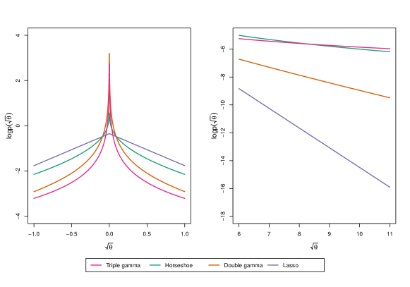
Figure 1: Marginal prior distribution of $\sqrt{\theta_{j}}$ under the triple gamma prior with $a^{\xi}=c^{\xi}=0.1$ with $\kappa^{2}_{B}=2$, in comparison to the Horseshoe prior with $\phi^{\xi}=1$, the double gamma prior with $a^{\xi}=0.1$ and $\kappa^{2}_{B}=2$ and the Lasso prior with $\kappa^{2}_{B}=2$. (a) On the left, spike of the marginal prior distributions. (b) On the right, tail of the marginal prior distributions.

In Figure 1 we can see the marginal prior distribution of $\sqrt{\theta_{j}}$ under the triple gamma prior $a^{\xi}=c^{\xi}=0.1$ and under other well-known shrinkage priors which are special cases of the triple gamma, see Table 1. Using Bitto and Frühwirth-Schnatter (2019, Footnote 3), Theorem 2.2 also allows to give a closed form for the prior $p(\theta_{j}|\phi^{\xi},a^{\xi},c^{\xi})=p(\sqrt{\theta_{j}}|\phi^{\xi},a^{\xi},c^{\xi})/\sqrt{\theta_{j}}$.

Global-local shrinkage priors are typically compared in terms of the concentration around the origin and the tail behaviour. For the triple gamma prior $p(\sqrt{\theta_{j}}|\phi^{\xi},a^{\xi},c^{\xi})$, the two shape parameters $a^{\xi}$ and $c^{\xi}$ play a crucial role in this respect, see Theorem 2.2 which is proven in Appendix A.

The triple gamma prior (9) satisfies the following:

• For $0<a^{\xi}<0.5$ and small values of $\sqrt{\theta_{j}}$,

  $$p(\sqrt{\theta_{j}}|\phi^{\xi},a^{\xi},c^{\xi})=\frac{\Gamma(\frac{1}{2}-a^{\xi})}{\sqrt{\pi}(2\phi^{\xi})^{a^{\xi}}B(a^{\xi},c^{\xi})}\left(\frac{1}{\sqrt{\theta_{j}}}\right)^{1-2a^{\xi}}+O(1).$$

• For $a^{\xi}=0.5$ and small values of $\sqrt{\theta_{j}}$,

  $$p(\sqrt{\theta_{j}}|\phi^{\xi},a^{\xi},c^{\xi})=\frac{1}{\sqrt{2\pi\phi^{\xi}}B(a^{\xi},c^{\xi})}\left(-\log\theta_{j}+\log(2\phi^{\xi})-\psi(c^{\xi}+{\frac{1}{2}})\right)+O(|\theta_{j}\log\theta_{j}|),$$

  where $\psi(\cdot)$ is the digamma function.

• For $a^{\xi}>0.5$,

  $$\lim_{\sqrt{\theta_{j}}\rightarrow 0}p(\sqrt{\theta_{j}}|\phi^{\xi},a^{\xi},c^{\xi})=\frac{\Gamma(c^{\xi}+{\frac{1}{2}})\Gamma(a^{\xi}-\frac{1}{2})}{\sqrt{2\pi\phi^{\xi}}B(a^{\xi},c^{\xi})\Gamma(a^{\xi}+c^{\xi})}.$$

• As $\sqrt{\theta_{j}}\rightarrow\infty$,

  $$p(\sqrt{\theta_{j}}|\phi^{\xi},a^{\xi},c^{\xi})=\frac{\Gamma(c^{\xi}+{\frac{1}{2}})(2\phi^{\xi})^{c^{\xi}}}{\sqrt{\pi}B(a^{\xi},c^{\xi})}\left(\frac{1}{\sqrt{\theta_{j}}}\right)^{2c^{\xi}+1}\left[1+O\left(\frac{1}{\theta_{j}}\right)\right].$$

From Theorem 2.2, Part (a) and (b), we find that the triple gamma prior $p(\sqrt{\theta_{j}}|\phi^{\xi},a^{\xi},c^{\xi})$ has a pole at the origin, if $a^{\xi}\leq 0.5$. According to Part (a), the pole is more pronounced, the closer $a^{\xi}$ gets to 0. For $a^{\xi}>0.5$, we find from Part (c) that $p(\sqrt{\theta_{j}}|\phi^{\xi},a^{\xi},c^{\xi})$ is bounded at zero by a positive upper bound which is finite, as long as $0<c^{\xi}<\infty$. Part (d) shows that the triple gamma prior $p(\sqrt{\theta_{j}}|\phi^{\xi},a^{\xi},c^{\xi})$ has polynomial tails, with the shape parameter $c^{\xi}$ controlling the tail index. Prior moments $\mbox{\rm E}((\sqrt{\theta_{j}})^{k}|\phi^{\xi},a^{\xi},c^{\xi})$ exist up to $k<2c^{\xi}$. Hence, the triple gamma prior has no finite moments for $c^{\xi}<1/2$.

Finally, additional useful representations of the triple gamma prior as a global-local shrinkage prior are summarized in Lemma 2.2 which is proven in Appendix A. Representations (a) shows that the triple gamma is an extension of the double gamma prior where the Gaussian prior $\sqrt{\theta_{j}}|\xi_{j}^{2}\sim\mathcal{N}(0,\xi_{j}^{2})$ is substituted by a heavier-tailed Student-$t$ prior, making the prior more robust to large values of $\sqrt{\theta_{j}}$. Representation (b) and (c) will be useful for MCMC inference in Section 4. Representations (c) and (d) show that for a triple gamma prior with finite $a^{\xi}$ and $c^{\xi}$, $\phi^{\xi}$ acts as a global shrinkage parameter, in addition to $2/\kappa_{B}^{2}$.

For $a^{\xi}>0$ and $c^{\xi}>0$, the triple gamma prior (5) has the following alternative representations:

$$\text{(a)}\quad\sqrt{\theta_{j}}|\tilde{\xi}_{j}^{2},c^{\xi},\kappa_{B}^{2}\sim t_{2c^{\xi}}\left(0,\frac{2}{\kappa_{B}^{2}}\tilde{\xi}_{j}^{2}\right),\quad\tilde{\xi}_{j}^{2}|a^{\xi}\sim\mathcal{G}\left(a^{\xi},a^{\xi}\right),$$ (10)

$$\text{(b)}\quad\sqrt{\theta_{j}}|\check{\xi}_{j}^{2},c^{\xi},\kappa_{B}^{2}\sim t_{2c^{\xi}}\left(0,\frac{2}{a^{\xi}\kappa_{B}^{2}}\check{\xi}_{j}^{2}\right),\quad\check{\xi}_{j}^{2}|a^{\xi}\sim\mathcal{G}\left(a^{\xi},1\right).$$ (11)

Additional representations for $0<a^{\xi}<\infty$ and $0<c^{\xi}<\infty$ based on $\phi^{\xi}=\frac{2c^{\xi}}{\kappa_{B}^{2}a^{\xi}}$ are

$$\text{(c)}\quad\sqrt{\theta_{j}}|\check{\xi}_{j}^{2},\check{\kappa}_{j}^{2},\phi^{\xi}\sim\mathcal{N}\left(0,\phi^{\xi}\check{\xi}_{j}^{2}/\check{\kappa}_{j}^{2}\right),\quad\check{\xi}_{j}^{2}|a^{\xi}\sim\mathcal{G}\left(a^{\xi},1\right),\quad\check{\kappa}_{j}^{2}|c^{\xi}\sim\mathcal{G}\left(c^{\xi},1\right),$$ (12)

$$\text{(d)}\quad\sqrt{\theta_{j}}|\tilde{\psi}^{2}_{j},\phi^{\xi}\sim\mathcal{N}\left(0,\phi^{\xi}\,\tilde{\psi}^{2}_{j}\right),\quad\tilde{\psi}^{2}_{j}|a^{\xi},c^{\xi}\sim\mathcal{BP}\left(a^{\xi},c^{\xi}\right),$$ (13)

where $\mathcal{BP}\left(a^{\xi},c^{\xi}\right)$ is the beta-prime distribution.

2.3 Relation of the triple gamma to other shrinkage priors

The triple gamma prior can be related to the very active research on shrinkage priors in a Bayesian framework in various ways. On the one hand, popular priors for variance parameters introduced as robust alternatives to the inverse gamma prior are special cases of the triple gamma, see Table 1. For instance, in (8), $\psi^{2}_{j}$ converges a.s. to 1, as $a^{\xi}\to\infty$ and $c^{\xi}\to\infty$, and the triple gamma reduces to a normal distribution for $\sqrt{\theta}_{j}$, applied for univariate TVP models (Frühwirth-Schnatter, 2004) and unobserved component state space model (Frühwirth-Schnatter and Wagner, 2010). For $c^{\xi}\to\infty$, $\mbox{\rm F}\left(2a^{\xi},2c^{\xi}\right)$ converges to the $\mathcal{G}\left(a^{\xi},a^{\xi}\right)$ distribution and the triple gamma reduces to the Bayesian Lasso for $a^{\xi}=1$ (Belmonte et al., 2014) and otherwise to the double gamma (Bitto and Frühwirth-Schnatter, 2019) applied in sparse TVP models.

Gelman (2006) introduced the half-$t$ and the half-Cauchy prior for variance parameters in hierarchical models, by assuming that $\sqrt{\theta}_{j}$ follows a “folded” $t$-distribution, i.e. a $t$-distribution truncated to $[0,\infty)$, see also Polson and Scott (2012). In (10), $\tilde{\xi}_{j}^{2}$ converges a.s. to 1 as $a^{\xi}\to\infty$ and the triple gamma reduces to a $t_{2c^{\xi}}$- distribution and to the Cauchy distribution for $c^{\xi}=1/2$, however without being “folded”, since we allow $\sqrt{\theta}_{j}$ to take on negative values. A half-$t_{\nu}$ with $\nu=2c^{\xi}$ and a triple gamma with $a^{\xi}=\infty$ obviously imply the same prior for $\theta_{j}$, so does the negative half matter? It matters, whenever inference is performed in a parametrization involving $\sqrt{\theta}_{j}$ such as the non-centered parametrization (2). Restricting the prior to the positive half will lead to automatic truncation of the full conditional posterior $p(\sqrt{\theta}_{j}|\tilde{\bm{\beta}}_{0},\ldots,\tilde{\bm{\beta}}_{T},\bm{y},\cdot)$, e.g. during MCMC sampling (see Section 4). If the positive and the negative mode of the marginal posterior $p(\sqrt{\theta}_{j}|\bm{y})$ are well-separated, then this will not matter. However, if the true value of $\theta_{j}$ is close to or equal to zero, then $p(\sqrt{\theta}_{j}|\bm{y})$ is concentrated at zero and truncation at 0 will introduce a bias, because the negative half is missing.

Prior for $\sqrt{\theta}_{j}$		$a^{\xi}$	$c^{\xi}$	$\kappa_{B}^{2}$	$\phi^{\xi}$
$\mathcal{N}\left(0,\psi^{2}_{j}\right),\psi^{2}_{j}\sim\mbox{GG}\left(a^{\xi},c^{\xi},\phi^{\xi}\right)$	normal-gamma-gamma	$a^{\xi}$	$c^{\xi}$	$\frac{2c^{\xi}}{\phi^{\xi}a^{\xi}}$	$\phi^{\xi}$
$\mathcal{N}\left(0,\frac{1}{\kappa_{j}}-1\right),\kappa_{j}\sim\mathcal{TPB}\left(a^{\xi},c^{\xi},\phi^{\xi}\right)$	generalized beta mixture	$a^{\xi}$	$c^{\xi}$	$\frac{2c^{\xi}}{\phi^{\xi}a^{\xi}}$	$\phi^{\xi}$
$\mathcal{N}\left(0,\psi^{2}_{j}\right),\psi^{2}_{j}\sim\mbox{SBeta2}\left(a^{\xi},c^{\xi},\phi^{\xi}\right)$	hierarchical scaled beta2	$a^{\xi}$	$c^{\xi}$	$\frac{2c^{\xi}}{\phi^{\xi}a^{\xi}}$	$\phi^{\xi}$
$\mathcal{DE}\left(0,\sqrt{2}\,\psi_{j}\right),\psi^{2}_{j}\sim\mathcal{G}\left(c^{\xi},\frac{1}{\lambda^{2}}\right)$	normal-exponential-gamma	$1$	$c^{\xi}$	$2\lambda^{2}c^{\xi}$	$\frac{1}{\lambda^{2}}$
$\mathcal{N}\left(0,\tau^{2}\psi^{2}_{j}\right),\psi_{j}\sim t_{1}$	Horseshoe	$\frac{1}{2}$	$\frac{1}{2}$	$\frac{2}{\tau^{2}}$	$\tau^{2}$
$\mathcal{N}\left(0,\frac{1}{\kappa_{j}}-1\right),\kappa_{j}\sim\mathcal{B}\left(1/2,1\right)$	Strawderman-Berger	$\frac{1}{2}$	1	4	1
$\mathcal{N}\left(0,\tau^{2}\tilde{\xi}_{j}\right),\tilde{\xi}_{j}\sim\mathcal{G}\left(a^{\xi},a^{\xi}\right)$	double gamma	$a^{\xi}$	$\infty$	$\frac{2}{\tau^{2}}$	-
$\mathcal{N}\left(0,\tau^{2}\tilde{\xi}_{j}\right),\tilde{\xi}_{j}\sim\mathcal{E}\left(1\right)$	Lasso	$1$	$\infty$	$\frac{2}{\tau^{2}}$	-
$t_{\nu}\left(0,\tau^{2}\right)$	half-$t$	$\infty$	$\frac{\nu}{2}$	$\frac{2}{\tau^{2}}$	-
$t_{1}\left(0,\tau^{2}\right)$	half-Cauchy	$\infty$	$\frac{1}{2}$	$\frac{2}{\tau^{2}}$	-
$\mathcal{N}\left(0,B_{0}\right)$	normal	$\infty$	$\infty$	$\frac{2}{B_{0}}$	-

Table 1: Priors on $\sqrt{\theta}_{j}$ which are equivalent to (top) or special cases of (bottom) the triple gamma prior.

On the other hand, the triple gamma prior is related to popular shrinkage priors in regression models. It extends the generalized beta mixture prior introduced by Armagan et al. (2011) for variable selection in regression models,

$$\beta_{j}|\xi_{j}^{2}\sim\mathcal{N}\left(0,\xi_{j}^{2}\right),\quad\xi_{j}^{2}\sim\mathcal{G}\left(a^{\xi},\lambda_{j}\right),\quad\lambda_{j}\sim\mathcal{G}\left(c^{\xi},\phi^{\xi}\right),$$

to variance selection in state space and TVP models. This is evident from rewriting (5) as $\xi_{j}^{2}\sim\mathcal{G}\left(a^{\xi},\lambda_{j}\right),\lambda_{j}\sim\mathcal{G}\left(c^{\xi},\phi^{\xi}\right)$. We exploit this relationship in Section 3.1 to investigate the shrinkage profile of a triple gamma prior. Using Armagan et al. (2011, Definition 2), the triple gamma prior can be written as

$$\sqrt{\theta}_{j}|\rho_{j}\sim\mathcal{N}\left(0,1/\rho_{j}-1\right),\quad\rho_{j}|a^{\xi},c^{\xi},\phi^{\xi}\sim\mathcal{TPB}\left(a^{\xi},c^{\xi},\phi^{\xi}\right),$$ (14)

where $\mathcal{TPB}\left(a^{\xi},c^{\xi},\phi^{\xi}\right)$ is the three-parameter beta (TPB) distribution with density:

$$p(\rho_{j})=\frac{1}{B(a^{\xi},c^{\xi})}(\phi^{\xi})^{c^{\xi}}\rho_{j}^{c^{\xi}-1}(1-\rho_{j})^{a^{\xi}-1}\left(1+(\phi^{\xi}-1)\rho_{j}\right)^{-(a^{\xi}+c^{\xi})}.$$ (15)

From (14) and (15), it becomes evident that the Strawderman-Berger prior $\sqrt{\theta}_{j}\sim\mathcal{N}\left(0,1/\rho_{j}-1\right)$, $\rho_{j}\sim\mathcal{B}\left(1/2,1\right)$ (Strawderman, 1971; Berger, 1980) is that special case of the triple gamma prior where $\phi^{\xi}=1$, $a^{\xi}=1/2$, and $c^{\xi}=1$.

The special case of a triple gamma, where $a^{\xi}=c^{\xi}=1/2$, corresponds to a Horseshoe prior (Carvalho et al., 2009, 2010) on $\sqrt{\theta}_{j}$ with global shrinkage parameter $\tau^{2}=2/\kappa_{B}^{2}$, since $\psi^{2}_{j}\sim\mbox{\rm F}\left(1,1\right)$ implies that $\psi_{j}\sim t_{1}$. The Horseshoe prior has been introduced for variable selection in regression models and has been shown to have excellent theoretical properties in this context for the “nearly black” case (van der Pas et al., 2014). The triple gamma is a generalization of the Horseshoe prior, with a similar shrinkage profile, however with much more mass close to the corner solutions. Most importantly, as will be discussed in Section 3.1, this leads to a BMA-type behaviour of the triple gamma prior for small values of $a^{\xi}$ and $c^{\xi}$.

The vast literature on shrinkage priors contains many more related priors. Rescaling $\xi_{j}^{2}=2/(\kappa_{B}^{2})\psi^{2}_{j}$ in (8), for instance, yields a representation involving a scaled beta2 distribution,

$$\sqrt{\theta}_{j}|\xi_{j}^{2}\sim\mathcal{N}\left(0,\xi_{j}^{2}\right),\qquad\xi_{j}^{2}|a^{\xi},c^{\xi},\phi^{\xi}\sim\mbox{SBeta2}\left(a^{\xi},c^{\xi},\phi^{\xi}\right),$$ (16)

as is easily derived from (31). The scaled beta2 was introduced by Pérez et al. (2017) in hierarchical models as a robust prior for scale parameters, $\sqrt{\theta}_{j}$, and variance parameters, $\theta_{j}$, alike. Based on (16), the triple gamma can be seen as a hierarchical extension of this prior which puts a scaled beta2 distribution on the scaling parameter $\xi_{j}^{2}$ of a Gaussian prior for $\sqrt{\theta}_{j}$, see Table 1. Griffin and Brown (2017) termed prior (16) gamma-gamma distribution, denoted by $\mbox{GG}\left(a^{\xi},c^{\xi},\phi\right)$.

For $a^{\xi}=1$, the triple gamma reduces to the normal-exponential-gamma which has a representation as a scale-mixture of double exponential $\mathcal{DE}\left(0,\sqrt{2}\psi_{j}\right)$-distributions, see Table 1. It has been considered for variable selection in regression models (Griffin and Brown, 2011) and locally adaptive B-spline models (Scheipl and Kneib, 2009). The R2-D2 prior suggested by Zhang et al. (2017) for high-dimensional regression models is another special case of the triple gamma. It reads

$$\beta_{j}\sim\mathcal{N}\left(0,\sigma^{2}\phi_{j}\omega\right),\quad(\phi_{1},\ldots,\phi_{d})\sim\mathcal{D}\left(a^{\tau},\ldots,a^{\tau}\right),\quad\omega\sim\mathcal{G}\left(a,\tau\right),\quad\tau\sim\mathcal{G}\left(b,1\right),$$

where $a=da^{\tau}$ and $\sigma^{2}$ is the residual error variance of the regression model. As shown by Zhang et al. (2017), this implies following prior for the coefficient of determination: $R^{2}\sim\mathcal{B}\left(a,b\right)$ which motivates holding $a$ fixed, while $a^{\tau}$ decrease as $d$ increases. Using that $\phi_{j}\omega\sim\mathcal{G}\left(a^{\tau},\tau\right)$, we can show that the R2-D2 prior is equivalent to following hierarchical normal gamma prior applied in Bitto and Frühwirth-Schnatter (2019) for TVP models:

$$\beta_{j}|\tau^{2}_{j}\sim\mathcal{N}\left(0,\tau^{2}_{j}\right),\quad\tau^{2}_{j}\sim\mathcal{G}\left(a^{\tau},a^{\tau}\lambda_{B}^{2}/2\right),\quad\lambda_{B}^{2}\sim\mathcal{G}\left(b,2\sigma^{2}/a^{\tau}\right).$$

The popular Dirichlet-Laplace prior, $\sqrt{\theta}_{j}|\psi_{j}\sim\mathcal{DE}\left(0,\psi_{j}\right)$, however, is not related to the triple gamma as the prior scale $\psi_{j}$ rather than $\psi^{2}_{j}$ follows a gamma distribution, see again Table 1.

2.4 Using the triple gamma for variance selection in TVP models

A challenging question is how to choose the parameters $a^{\xi}$, $c^{\xi}$ and $\kappa_{B}^{2}$ or $\phi^{\xi}$ of the triple gamma prior in the context of variance selection for TVP models. In addition, in a TVP context, the shrinkage parameters $a^{\tau}$, $c^{\tau}$ and $\lambda_{B}^{2}$ or $\phi^{\tau}=2c^{\tau}/(a^{\tau}\lambda_{B}^{2})$ for the prior (7) of the initial values have to be selected.

In high-dimensional settings it is appealing to have a prior that addresses two major issues: first, high concentration around the origin to favor strong shrinkage of small variances toward zero; second, heavy tails to introduce robustness to large variances and to avoid over-shrinkage. For the triple gamma prior, both issues are addressed through the choice of $a^{\xi}$ and $c^{\xi}$, see Theorem 2.2. First of all, we need values $0<a^{\xi}\leq 0.5$ to induce a pole at 0. Second, values of $0<c^{\xi}<0.5$ will lead to very heavy tails. For very small values of $a^{\xi}$ and $c^{\xi}$, the triple Gamma is a proper prior that behaves nearly as the improper normal-Jeffrey’s prior (Figueiredo, 2003), where $p(\sqrt{\theta}_{j})\propto 1/\sqrt{\theta}_{j}$ and $p(\rho_{j})\propto\rho_{j}^{-1}(1-\rho_{j})^{-1}$.

Ideally, we would place a hyper prior distribution on all shrinkage parameters which would allow us to learn the global and the local degree of sparsity, both for the variances and the initial values. Such a hierarchical triple gamma prior introduces dependence among the local shrinkage parameters $\xi^{2}_{1},\ldots,\xi^{2}_{d}$ in (5) and, consequently, among $\theta_{1},\ldots,\theta_{d}$ in the joint (marginal) prior $p(\theta_{1},\ldots,\theta_{d})$. Introducing such dependence is desirable in that it allows to learn the degree of variance sparsity in TVP models, meaning that how much a variance is shrunken toward zero depends on how close the other variances are to zero. However, first naïve approaches with rather uninformative, independent priors on $\kappa_{B}^{2}$, $a^{\xi}$, $c^{\xi}$ and $\lambda_{B}^{2}$, $a^{\tau}$, $c^{\tau}$ were not met with much success and we found it necessary to carefully design appropriate hyper priors.

Hierarchical versions of the Bayesian Lasso (Belmonte et al., 2014) and the double gamma prior (Bitto and Frühwirth-Schnatter, 2019) in TVP models are based on the gamma prior $\kappa_{B}^{2}\sim\mathcal{G}\left(d_{1},d_{2}\right)$. Interestingly, this choice can be seen as a heavy-tailed extension of both priors, where each marginal density $p(\sqrt{\theta}_{j}|d_{1},d_{2})$ follows a triple gamma prior with the same parameter $a^{\xi}$ (being equal to one for the Bayesian Lasso) and tail index $c^{\xi}=d_{1}$. In light of this relationship, it is not surprising that very small values of $d_{1}$ were applied in these papers to ensure heavy tails of $p(\sqrt{\theta}_{j}|d_{1},d_{2})$. Since a triple gamma prior has already heavy tails, we choose a different hyperprior in the present paper.

For the case $a^{\xi}=c^{\xi}=1/2$, the global shrinkage parameter $\tau$ of the Horseshoe prior typically follows a Cauchy prior, $\tau\sim t_{1}$ (Carvalho et al., 2009; Bhadra et al., 2017), see also Bhadra et al. (2019, Section 5). The relationship $\phi^{\xi}=2/\kappa_{B}^{2}=\tau^{2}$ between the various global shrinkage parameters (see Table 1) implies in this case $\phi^{\xi}\sim\mbox{\rm F}\left(1,1\right)$ or, equivalently, $\kappa^{2}_{B}/2\sim\mbox{\rm F}\left(1,1\right)$.

For a triple gamma prior with arbitrary $a^{\xi}$ and $c^{\xi}$, this is a special case of the following prior:

$$\left.\frac{\kappa_{B}^{2}}{2}\right|a^{\xi},c^{\xi}\sim\mbox{\rm F}\left(2a^{\xi},2c^{\xi}\right),$$ (17)

which will be motivated in Section 3.2. Under this prior, the triple gamma prior exhibits a BMA-like behavior with a uniform prior on an appropriately defined model size (see Theorem 3.2). Prior (17) is equivalent with following representations:

$$\kappa_{B}^{2}|a^{\xi}\sim\mathcal{G}\left(a^{\xi},d_{2}\right),\qquad d_{2}|a^{\xi},c^{\xi}\sim\mathcal{G}\left(c^{\xi},\dfrac{2c^{\xi}}{a^{\xi}}\right),$$ (18)

$$\phi^{\xi}|a^{\xi},c^{\xi}\sim\mathcal{BP}\left(c^{\xi},a^{\xi}\right).$$

Concerning $a^{\xi}$ and $c^{\xi}$, we choose the following priors:

$$2a^{\xi}\sim\mathcal{B}(\alpha_{a^{\xi}},\beta_{a^{\xi}}),\qquad 2c^{\xi}\sim\mathcal{B}(\alpha_{c^{\xi}},\beta_{c^{\xi}}).$$ (19)

Hence, we are restricting the support of $a^{\xi}$ and $c^{\xi}$ to $(0,0.5)$, following the insights brought to us by Theorem 2.2.

We follow a similar strategy for the parameters $a^{\tau}$, $c^{\tau}$ and $\lambda_{B}^{2}$ ($\phi^{\tau}$) of the prior (7):

$$\left.\frac{\lambda_{B}^{2}}{2}\right|a^{\tau},c^{\tau}\sim\mbox{\rm F}\left(2a^{\tau},2c^{\tau}\right),\quad$$ (20)

which is equivalent with $\lambda_{B}^{2}|a^{\tau}\sim\mathcal{G}\left(a^{\tau},e_{2}\right)$, $e_{2}|c^{\tau}\sim\mathcal{G}\left(c^{\tau},2c^{\tau}/a^{\tau}\right)$, and $\phi^{\tau}|a^{\tau},c^{\tau}\sim\mathcal{BP}\left(c^{\tau},a^{\tau}\right)$.

An interesting special case is the “symmetric”  triple gamma, where $a^{\xi}=c^{\xi}$. Despite this constraint, the favourable shrinkage behaviour is preserved and decreasing $a^{\xi}=c^{\xi}$ toward zero simultaneously leads to a high concentration around the origin and a heavy-tailed behaviour. For a symmetric triple gamma prior, $\phi^{\xi}=2/\kappa_{B}^{2}$ is independent of $a^{\xi}$ and $c^{\xi}$ and the two global shrinkage parameters are related through $\phi^{\xi}=2/\kappa_{B}^{2}$. This induces shrinkage profiles that are symmetric around 1/2, see Section 3.1. Interestingly, a symmetric triple gamma resolves the question whether to choose a gamma or an inverse gamma prior for a variance parameter $\psi^{2}_{j}$. It implies the same symmetric beta-prime distribution on the variance, $\psi^{2}_{j}\sim\mbox{\rm F}\left(2a^{\xi},2a^{\xi}\right)=\mathcal{BP}\left(a^{\xi},a^{\xi}\right)$, and the information, $(\psi^{2}_{j})^{-1}\sim\mathcal{BP}\left(a^{\xi},a^{\xi}\right)$, and can be represented as a gamma prior with the scale arising from an inverse gamma prior or, equivalently, as an inverse gamma prior with the scale arising from a gamma prior:

$$\psi^{2}_{j}=\check{\xi}_{j}^{2}\times\frac{1}{\check{\kappa}_{j}^{2}},\quad(\psi^{2}_{j})^{-1}=\check{\kappa}_{j}^{2}\times\frac{1}{\check{\xi}_{j}^{2}},\qquad\check{\xi}_{j}^{2}\sim\mathcal{G}\left(a^{\xi},1\right),\,\,\check{\kappa}_{j}^{2}\sim\mathcal{G}\left(a^{\xi},1\right).$$

3 Shrinkage profiles and BMA-like behavior

3.1 Shrinkage profiles

In the sparse normal-means problem where $\bm{y}|\bm{\beta}\sim\mathcal{N}_{d}\left(\bm{\beta},\sigma^{2}{{\mathbf{I}}}_{d}\right)$ and $\sigma^{2}=1$, the parameter $\rho_{j}=1/(1+\psi^{2}_{j})$ appearing in (14) is known as shrinkage factor and plays a fundamental role for comparing different shrinkage priors, as $\rho_{j}$ determines shrinkage toward 0.

Also in a variance selection context, it is evident from (14) that values of $\rho_{j}\approx 0$ will introduce no shrinkage on $\theta_{j}$, whereas values of $\rho_{j}\approx 1$ will introduce strong shrinkage of $\theta_{j}$ toward 0. Hence, the prior $p(\rho_{j})$, also called shrinkage profile, will play an instrumental role in the behaviour of different shrinkage priors. Following Carvalho et al. (2010), shrinkage priors are often compared in terms of the prior they imply on $\rho_{j}$, i.e. how they handle shrinkage for small “observations” (in our case innovations) and how robust they are to large “observations”. Note that we ideally want a shrinkage profile that has a pole in zero (heavy tails to avoid over-shrinking signals) and a pole in one (spikiness to shrink noise). The Horseshoe prior, e.g., implies $\rho_{j}\sim\mathcal{B}\left(1/2,1/2\right)$ which is a shrinkage profile that takes this much desired form of a “Horseshoe”, see Figure 2.

For the triple gamma prior, the shrinkage profile is given by the three-parameter beta prior $p(\rho_{j})$ provided in (15). For $\phi^{\xi}=1$, $\rho_{j}\sim\mathcal{B}\left(c^{\xi},a^{\xi}\right)$ and $\kappa_{B}^{2}=2c^{\xi}/a^{\xi}$. Choosing small values $a^{\xi}<<1$ will put prior mass close to 1, choosing small values $c^{\xi}<<1$ will put prior mass close to 0, whereas values for both $a^{\xi}$ and $c^{\xi}$ smaller than one will induce the form of a Horseshoe prior for $\rho_{j}$. Evidently, for $\phi^{\xi}=1$, a symmetric triple gamma prior with $a^{\xi}=c^{\xi}$ implies a Horseshoe prior for $\rho_{j}$ that is symmetric around 0.5. This is illustrated in Figure 2 for a symmetric triple gamma with $a^{\xi}=c^{\xi}=0.1$.

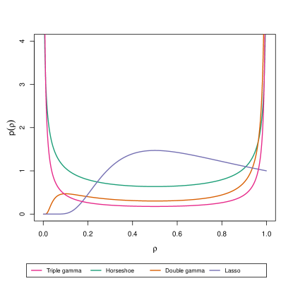
Figure 2: Marginal univariate shrinkage profile under the triple gamma prior with $a^{\xi}=c^{\xi}=0.1$, in comparison to the Horseshoe prior, the double gamma prior with $a^{\xi}=0.1$ the Lasso prior. $\kappa^{2}_{B}=2$ for all the prior specifications.

In Figure 2 we can also see the shrinkage profile for the Bayesian Lasso and the double gamma, which correspond to a triple gamma where $c^{\xi}\rightarrow\infty$. For the Bayesian Lasso with $a^{\xi}=1$ it is clear that the shrinkage profile $p(\rho_{j})$ converges to a constant for $\rho_{j}\to 1$, while there is no mass around $\rho_{j}=0$. This means that this prior tends to over-shrink signals, while not shrinking the noise completely to zero. A double gamma prior with $a^{\xi}<1$ has the potential to shrink the noise completely to zero, as $p(\rho_{j})$ has a pole at $\rho_{j}=1$, but $p(\rho_{j})$ has also zero mass around $\rho_{j}=0$, meaning the prior encourages over-shrinking of signals.

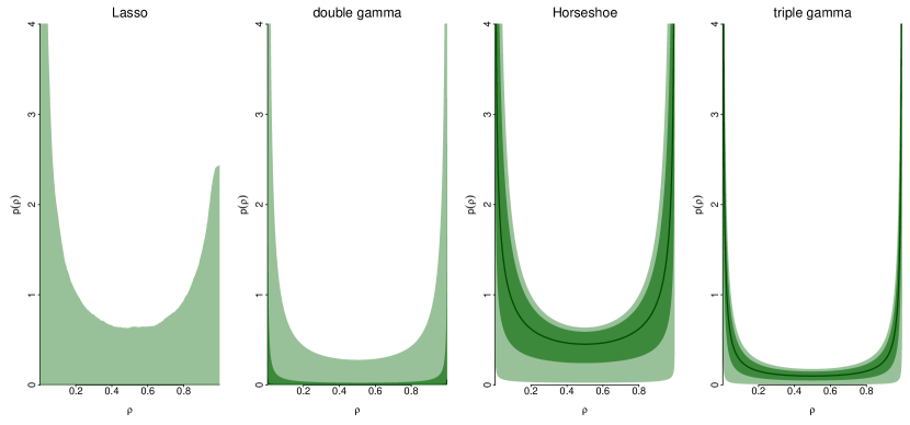
Figure 3: “Prior density” of shrinkage profiles for (from left to right) Lasso prior, double gamma prior with $a^{\xi}=0.2$, Horseshoe prior and triple gamma prior with $a^{\xi}=c^{\xi}=0.1$, when $\kappa_{B}^{2}$ is random. The solid line is the median, while the shaded areas represent 50% and 95 % prior credible bands. We have used $\kappa_{B}^{2}\sim\mathcal{G}\left(0.01,0.01\right)$ for the Lasso and the double gamma, $2/\kappa_{B}^{2}\sim\mbox{\rm F}\left(1,1\right)$ for the Horseshoe and $2/\kappa_{B}^{2}\sim\mbox{\rm F}\left(0.2,0.2\right)$ for the triple gamma.

When we make $\kappa_{B}^{2}$ random, we obtain a “prior density” of shrinkage profiles, see Figure 3. We can see that such hierarchical versions of the Lasso and the double gamma have shrinkage profiles that resemble the ones of the Horseshoe and the triple gamma. We have used $\kappa_{B}^{2}\sim\mathcal{G}\left(0.01,0.01\right)$ for the Lasso and the double gamma, $2/\kappa_{B}^{2}\sim\mbox{\rm F}\left(1,1\right)$ for the Horseshoe and $2/\kappa_{B}^{2}\sim\mbox{\rm F}\left(0.2,0.2\right)$ for the triple gamma, see Section 2.4.

3.2 BMA-type behaviour

From the perspective of Bayesian model averaging (BMA), an ideal approach for handling sparsity in TVP models would be the use of discrete mixture priors as suggested in Frühwirth-Schnatter and Wagner (2010),

$$p(\sqrt{\theta}_{j})=(1-\pi)\delta_{0}+\pi\cdot p_{\mbox{\tiny slab}}(\sqrt{\theta}_{j}),$$ (21)

with $\delta_{0}$ being a Dirac measure at 0, while $p_{\mbox{\tiny slab}}(\sqrt{\theta}_{j})$ is the prior for non-zero variances. In terms of shrinkage profiles, the discrete mixture prior (21) has a spike at $\rho_{j}=1$, with probability $1-\pi$, and a lot of prior mass at $\rho_{j}=0$, provided that the tails of $p_{\mbox{\tiny slab}}(\sqrt{\theta}_{j})$ are heavy enough. The mixture prior (21) is considered the “gold standard” in BMA, both theoretically and empirically, see e.g. Johnstone and Silverman (2004). However, MCMC inference under this prior is extremely challenging. As opposed to this, MCMC inference for the triple gamma prior is straightforward, see Section 4.

In this section, we relate the triple gamma prior to BMA based on the discrete mixture prior (21). An interesting insight is that the triple gamma prior shows a very similar behaviour as a discrete mixture prior, if both $a^{\xi}$ and $c^{\xi}$ approach zero. This induces a BMA-type behaviour on the joint shrinkage profile $p(\rho_{1},\ldots,\rho_{d})$, with a spike at all corner solutions, where some $\rho_{j}$ are very close to one, whereas the remaining ones very close to zero.

The bivariate shrinkage profiles shown in Figure 4 give us some intuition about the convergence of a symmetric triple gamma prior with $a^{\xi}=c^{\xi}\rightarrow 0$ toward a discrete spike and slab mixture. As opposed to the Lasso and the double gamma prior, the Horseshoe and the triple gamma prior put nearly all prior mass on the “corner solutions”, which correspond to the four possibilities (a) $\rho_{1}=\rho_{2}=0$, i.e. no shrinkage on $\theta_{1}$ and $\theta_{2}$, (b) $\rho_{1}=1,\rho_{2}=0$, i.e. shrinkage of $\theta_{1}$ toward 0 and no shrinkage on $\theta_{2}$, (c) $\rho_{1}=0,\rho_{2}=1$, i.e. shrinkage of $\theta_{1}$ toward 0 and no shrinkage on $\theta_{2}$, and (d) $\rho_{1}=\rho_{2}=1$, i.e. shrinkage of both $\theta_{1}$ and $\theta_{2}$ toward 0.

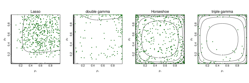
Figure 4: Bivariate shrinkage profile $p(\rho_{1},\rho_{2})$ for (from left to right) the Lasso prior, the double gamma prior with $a^{\xi}=0.1$, the Horseshoe prior, and the triple gamma prior with $a^{\xi}=c^{\xi}=0.1$, with $\kappa^{2}_{B}=2$ for all the priors. The contour plots of the bivariate shrinkage profile are shown, together with 500 samples from the bivariate prior distribution of the shrinkage parameters.

A very important aspect of BMA is the one of choosing a prior for the model dimension, $K$, see e.g. Fernández et al. (2001) and Ley and Steel (2009). In the discrete mixture prior (21), the distribution of $K$ depends on the choice of $\pi$. Fixing $\pi$ corresponds to a very informative prior on the model dimension, for example $\pi=0.5$ assigns more prior probability to models of dimension $d/2$ and lower prior probability to empty or full models. In fact, let $\delta_{j}$ be the indicator that tells us if the $j$-th coefficient is included in the model, then we have that $K=\sum_{j=1}^{d}{\delta_{j}}\sim\mbox{\rm BiNom}\left(d,\pi\right)$. Placing a uniform prior for $\pi$ has been shown to be a good choice, since it corresponds to placing a prior on $K$ which is uniform on $\{0,\ldots,d\}$. Note that $\pi$ will be learned using information from all the variables, that it is a global parameter and will adapt to the degree of sparsity.

Following ideas in Carvalho et al. (2009), we believe that a natural way to perform variable selection in the continuous shrinkage prior framework is though thresh-holding. Specifically, we say that when $(1-\rho_{j})>0.5$, or $\rho_{j}<0.5$, the variable is included, otherwise it is not. Notice that this classification via thresh-holding makes perfectly sense in the case of a triple gamma of which the Horseshoe is a special case, but less so for a Lasso or double gamma prior, even if the shrinkage profile shows a Horseshoe-like behaviour for hierarchical versions of these priors (see again Figure 3). Notice that this implies a prior on the model dimension $K$. Specifically,

$$K=\sum_{j=1}^{d}I\{\rho_{j}<0.5\}\sim\mbox{\rm BiNom}\left(d,\pi^{\xi}\right),\quad\pi^{\xi}=\mbox{\rm Pr}(\rho_{j}<0.5),$$ (22)

where $\rho_{j}|a^{\xi},\phi^{\xi}\sim\mathcal{TPB}\left(a^{\xi},b^{\xi},\phi^{\xi}\right)$, see (15). The choice of $\phi^{\xi}$ (or $\kappa^{2}_{B}$) will strongly impact the prior on $K$. For a symmetric triple gamma with $a^{\xi}=c^{\xi}$, for instance, and fixed $\phi^{\xi}=1$, that is $\kappa^{2}_{B}=2$, we obtain $K\sim\mbox{\rm BiNom}\left(d,0.5\right)$, since $\pi^{\xi}=0.5$ regardless of $a^{\xi}$. Hence, we have to face similar problems as with fixing $\pi=0.5$ for the discrete mixture prior (21).

Placing a hyper prior on $\phi^{\tau}$ and $\phi^{\xi}$ or, equivalently on, $\lambda_{B}^{2}$ and $\kappa^{2}_{B}$, as we did in Section 2.4, is as instrumental for BMA-type variable and variance selection for the triple gamma prior, as is making $\pi$ random for the discrete mixture prior (21). Ideally, we would like to have a uniform distribution on the model size $K$. We show in Theorem 3.2 that the hyperprior for $\kappa_{B}^{2}$ defined in (17) achieves exactly this goal, since $\pi^{\xi}$ is uniformly distributed, see Appendix A for a proof.

For a hierarchical triple gamma prior with fixed $a^{\xi}>0$ and $c^{\xi}>0$ the probability $\pi^{\xi}$ defined in (22) follows a uniform distribution, $\pi^{\xi}\sim\mathcal{U}\left[0,1\right]$, under the hyper prior

$$\left.\frac{\kappa_{B}^{2}}{2}\right|a^{\xi},c^{\xi}\sim\mbox{\rm F}\left(2a^{\xi},2c^{\xi}\right),$$ (23)

or, equivalently, under the hyper prior

$$\phi^{\xi}|a^{\xi},c^{\xi}\sim\mathcal{BP}\left(c^{\xi},a^{\xi}\right).$$ (24)

4 MCMC algorithm

Let $\bm{y}=(y_{1},\ldots,y_{T})$ be the vector of time series observations and let $\bm{z}$ be the set of all latent variables and unknown model parameters in a TVP model. Moreover, let $\bm{z}_{-x}$ denote the set of all unknowns but $x$. Bayesian inference based on MCMC sampling from the posterior $p(\bm{z}|\bm{y})$ is summarized in Algorithm 1. The hierarchical priors introduced in Section 2.4 are employed, where $(a^{\tau},c^{\tau},\lambda_{B}^{2})$ follow (20), $(a^{\xi},c^{\xi})$ follow (19), and $\kappa_{B}^{2}$ follows (17). For certain sampling steps, the hierarchical representation (18) is used for $\kappa_{B}^{2}$, and similarly for $\lambda_{B}^{2}$.

Algorithm 1 extends several existing algorithms such as the MCMC schemes introduced for the Horseshoe prior by Makalic and Schmidt (2016) and for the double gamma prior by Bitto and Frühwirth-Schnatter (2019). We exploit various representations of the triple gamma prior given in Lemma 2.2 and choose representation (12) as the baseline representation of our MCMC algorithm:

$$\beta_{j}|\check{\tau}_{j}^{2},\check{\lambda}_{j}^{2},\phi^{\tau}\sim\mathcal{N}\left(0,\phi^{\tau}\check{\tau}_{j}^{2}/\check{\lambda}_{j}^{2}\right),\quad\check{\tau}_{j}^{2}|a^{\tau}\sim\mathcal{G}\left(a^{\tau},1\right),\quad\check{\lambda}_{j}^{2}|c^{\tau}\sim\mathcal{G}\left(c^{\tau},1\right),$$

$$\sqrt{\theta_{j}}|\check{\xi}_{j}^{2},\check{\kappa}_{j}^{2},\phi^{\xi}\sim\mathcal{N}\left(0,\phi^{\xi}\check{\xi}_{j}^{2}/\check{\kappa}_{j}^{2}\right),\quad\check{\xi}_{j}^{2}|a^{\xi}\sim\mathcal{G}\left(a^{\xi},1\right),\quad\check{\kappa}_{j}^{2}|c^{\xi}\sim\mathcal{G}\left(c^{\xi},1\right),$$

where $\phi^{\tau}=2c^{\tau}/(\lambda_{B}^{2}a^{\tau})$ and $\phi^{\xi}=2c^{\xi}/(\kappa_{B}^{2}a^{\xi})$. All conditional distributions in our MCMC scheme are available in closed form, expect the ones for $a^{\xi}$, $c^{\xi}$, $a^{\tau}$ and $c^{\tau}$, for which we will resort to a MH step within Gibbs. Several conditional distributions are the same as for the double gamma prior and we apply Algorithm 1 of Bitto and Frühwirth-Schnatter (2019). We provide more details on the derivation of the various densities in Appendix B.

Algorithm 1.

MCMC inference for TVP models under the triple gamma prior Choose starting values for all global and local shrinkage parameters, i.e. $(a^{\tau},c^{\tau},\lambda_{B}^{2},a^{\xi},c^{\xi},\kappa_{B}^{2})$ and $\{\check{\tau}^{2}_{j},\check{\lambda}_{j}^{2},\check{\xi}_{j}^{2},\check{\kappa}_{j}^{2}\}_{j=1}^{d}$, and repeat the following steps:

• Define for $j=1,\ldots,d$, $\tau^{2}_{j}=\phi^{\tau}\check{\tau}^{2}_{j}/\check{\lambda}_{j}^{2}$ and $\xi^{2}_{j}=\phi^{\xi}\check{\xi}_{j}^{2}/\check{\kappa}_{j}^{2}$ and sample from the posterior $p(\tilde{\bm{\beta}}_{0},\ldots,\tilde{\bm{\beta}}_{T},\beta_{1},\ldots,\beta_{d},\sqrt{\theta_{1}},\ldots,\sqrt{\theta_{d}}|\{\xi_{j}^{2},\tau_{j}^{2}\}_{j=1}^{d},\bm{y})$ using Algorithm 1, Steps (a), (b), and (c) in Bitto and Frühwirth-Schnatter (2019). In the homoscedastic case, use Step (f) of this algorithm to sample from $\sigma^{2}|\bm{z}_{-\sigma^{2}},\bm{y}$. For the SV model (3), sample the parameters $\mu$, $\phi$, and $\sigma_{\eta}^{2}$ as in Kastner and Frühwirth-Schnatter (2014), e.g., using the R-package stochvol (Kastner, 2016).

• Use the prior $p(\sqrt{\theta}_{j}|\check{\kappa}_{j}^{2},a^{\xi},c^{\xi})$, marginalized w.r.t. $\check{\xi}_{j}^{2}$, to sample $a^{\xi}$ from $p(a^{\xi}|\bm{z}_{-a^{\xi}},\bm{y})$ via a random walk MH step on $z=\log(a^{\xi}/(0.5-a^{\xi}))$. Propose $a^{\xi,(*)}=0.5\text{e}^{z^{*}}/(1+\text{e}^{z^{*}})$, where $z^{*}\sim\mathcal{N}\left(z^{(m-1)},v^{2}\right)$ and $z^{(m-1)}=\log(a^{\xi,(m-1)}/(0.5-a^{\xi,(m-1)}))$ depends on the previous value $a^{\xi,(m-1)}$ of $a^{\xi}$, accept $a^{\xi,(*)}$ with probability

  $$\min\left\{1,\frac{q_{a}(a^{\xi,(*)})}{q_{a}(a^{\xi,(m-1)})}\right\},\qquad{q_{a}(a^{\xi})=p(a^{\xi}|\bm{z}_{-a^{\xi}},\bm{y})\,a^{\xi}(0.5-a^{\xi})},$$

  and update $\phi^{\xi}=2c^{\xi}/(\kappa_{B}^{2}a^{\xi})$. Explicit forms for $p(a^{\xi}|\bm{z}_{-a^{\xi}},\bm{y})$ and $\log q_{a}(a^{\xi})$ are provided in (32) and (34).

  Similarly, use the prior $p(\beta_{j}|\check{\lambda}_{j}^{2},a^{\tau},c^{\tau})$, marginalized w.r.t. to $\check{\tau}_{j}^{2}$, to sample $a^{\tau}$ via a MH step and update $\phi^{\tau}=2c^{\tau}/(a^{\tau}\lambda_{B}^{2})$.

• Sample $\check{\xi}_{j}^{2}$, $j=1,\ldots,d$, from a generalized inverse Gaussian distribution, see (36):

  $$\check{\xi}_{j}^{2}|\check{\kappa}_{j}^{2},\theta_{j},a^{\xi},\phi^{\xi}\sim\mathcal{GIG}\left(a^{\xi}-\frac{1}{2},2,\dfrac{\check{\kappa}_{j}^{2}\theta_{j}}{\phi^{\xi}}\right).$$ (25)

  Similarly, update $\check{\tau}_{j}^{2}$, $j=1,\ldots,d$, conditional on $a^{\tau}$:

  $$\check{\tau}_{j}^{2}|\beta_{j},\check{\lambda}_{j}^{2},a^{\tau},\phi^{\tau}\sim\mathcal{GIG}\left(a^{\tau}-\frac{1}{2},2,\dfrac{\check{\lambda}_{j}^{2}\beta_{j}^{2}}{\phi^{\tau}}\right).$$

• Use the marginal Student-$t$ distribution $p(\sqrt{\theta}_{j}|\check{\xi}_{j}^{2},c^{\xi},\kappa_{B}^{2})$ given in (11) to sample $c^{\xi}$ from $p(c^{\xi}|\bm{z}_{-c^{\xi}},\bm{y})$ via a random walk MH step on $z=\log({c^{\xi}}/{(0.5-c^{\xi})})$. Propose $c^{\xi,(*)}=0.5\text{e}^{z^{*}}/(1+\text{e}^{z^{*}})$, where $z^{*}\sim\mathcal{N}\left(z^{(m-1)},v^{2}\right)$ and $z^{(m-1)}=\log(c^{\xi,(m-1)}/(0.5-c^{\xi,(m-1)}))$ depends on the previous value $c^{\xi,(m-1)}$ of $c^{\xi}$, accept $c^{\xi,(*)}$ with probability

  $$\min\left\{1,\frac{q_{c}(c^{\xi,(*)})}{q_{c}(c^{\xi,(m-1)})}\right\},\qquad{q_{c}(c^{\xi})=p(c^{\xi}|\bm{z}_{-c^{\xi}},\bm{y})\,c^{\xi}(0.5-c^{\xi})},$$

  and update $\phi^{\xi}=\frac{2c^{\xi}}{\kappa_{B}^{2}a^{\xi}}$. Explicit forms for $p(c^{\xi}|\bm{z}_{-c^{\xi}},\bm{y})$ and $\log q_{c}(c^{\xi})$ are provided in (37) and (38).

  Similarly, to sample $c^{\tau}$ via a MH step use the marginal distribution of $\beta_{j}|\check{\tau}_{j}^{2},a^{\tau},c^{\tau}$ with respect to $\check{\lambda}_{j}^{2}$ and update $\phi^{\tau}=2c^{\tau}/(a^{\tau}\lambda_{B}^{2})$.

• Sample $\check{\kappa}_{j}^{2}$, for $j=1,\ldots,d$, from following gamma distribution, see (40):

  $$\check{\kappa}_{j}^{2}|\theta_{j},\check{\xi}_{j}^{2},c^{\xi},\phi^{\xi}\sim\mathcal{G}\left(1/2+c^{\xi},\dfrac{\theta_{j}}{2\phi^{\xi}\check{\xi}_{j}^{2}}+1\right).$$ (26)

  Similarly, update $\check{\lambda}_{j}^{2}$, $j=1,\ldots,d$, conditional on $c^{\tau}$:

  $$\check{\lambda}_{j}^{2}|\beta_{j},\check{\tau}_{j}^{2},c^{\tau},\phi^{\tau}\sim\mathcal{G}\left(1/2+c^{\tau},\dfrac{\beta^{2}_{j}}{2\phi^{\tau}\check{\tau}_{j}^{2}}+1\right).$$

• Sample $d_{2}$ from $d_{2}|a^{\xi},c^{\xi},\kappa_{B}^{2}\sim\mathcal{G}\left({a^{\xi}+c^{\xi}},\kappa_{B}^{2}+\frac{2c^{\xi}}{a^{\xi}}\right)$, see (41); sample from $\kappa_{B}^{2}$ from following gamma distribution,

  $$\kappa_{B}^{2}|\{\theta_{j},\check{\kappa}^{2}_{j},\check{\xi}_{j}^{2}\}_{j=1}^{d},a^{\xi},c^{\xi},d_{2}\sim\mathcal{G}\left({\frac{d}{2}+a^{\xi}},\dfrac{a^{\xi}}{4c^{\xi}}\sum_{j=1}^{d}\frac{\check{\kappa}_{j}^{2}}{\check{\xi}_{j}^{2}}\theta_{j}+d_{2}\right),$$ (27)

  see (42), and update $\phi^{\xi}=\frac{2c^{\xi}}{\kappa_{B}^{2}a^{\xi}}$.

  Similarly, sample $e_{2}$ from $e_{2}|a^{\tau},c^{\tau},\lambda_{B}^{2}\sim\mathcal{G}\left({a^{\tau}+c^{\tau}},\lambda_{B}^{2}+\frac{2c^{\tau}}{a^{\tau}}\right)$, sample $\lambda_{B}^{2}$ from

  $$\lambda_{B}^{2}|\{\beta_{j},\check{\lambda}^{2}_{j},\check{\tau}_{j}^{2}\}_{j=1}^{d},a^{\tau},c^{\tau},e_{2}\sim\mathcal{G}\left({\frac{d}{2}+a^{\tau}},\dfrac{a^{\tau}}{4c^{\tau}}\sum_{j=1}^{d}\frac{\check{\lambda}_{j}^{2}}{\check{\tau}_{j}^{2}}\beta^{2}_{j}+e_{2}\right),$$

  and update $\phi^{\tau}=2c^{\tau}/(a^{\tau}\lambda_{B}^{2})$.

The MCMC scheme in Algorithm 1 is not a full conditional scheme, as several steps are based on partially marginalized distributions. That means that the sampling order matters. For instance, in Step (b), we marginalize w.r.t. $\check{\xi}_{1}^{2},\ldots,\check{\xi}_{d}^{2}$, hence we need to update $\check{\xi}_{1}^{2},\ldots,\check{\xi}_{d}^{2}$ after sampling $a^{\xi}$, before we update $c^{\xi}$ in Step (d) conditional on $\check{\xi}_{1}^{2},\ldots,\check{\xi}_{d}^{2}$. Similarly, due to marginalization in Step (d), we need to update $\check{\kappa}_{1}^{2},\ldots,\check{\kappa}_{d}^{2}$, before we update $d_{2}$ in Step (f). Furthermore, both Step (b) and Step (d) are based on the marginal prior of $\kappa_{B}^{2}$, given in (17). Hence, in Step (f), $d_{2}$ has to be updated from $d_{2}|a^{\xi},c^{\xi},\kappa_{B}^{2}$, before $\kappa_{B}^{2}$ is updated conditional on $d_{2}$.

For a symmetric triple gamma prior, where $a^{\xi}=c^{\xi}$, the MCMC scheme in Algorithm 1 has to be modified only slightly. Either $q_{a}(a^{\xi})$ in Step (b) is adjusted and Step (d) is skipped, setting $c^{\xi}=a^{\xi}$, or $q_{c}(c^{\xi})$ in Step (d) is adjusted and Step (b) is skipped, setting $a^{\xi}=c^{\xi}$. In Appendix B, we provide details in (43) for the first case and in (44) for the second case. Similar modifications are needed, if $a^{\tau}=c^{\tau}$. All other steps in Algorithm 1 remain the same for $a^{\xi}=c^{\xi}$ and/or $a^{\tau}=c^{\tau}$.

5 Applications to TVP-VAR-SV models

5.1 Model

Consider an -dimensional time series, $\bm{Y}_{1},\ldots,\bm{Y}_{T}$. The joint dynamics of such time series can be modeled through a time-varying parameter vector autoregressive model with stochastic volatility (TVP-VAR-SV). Since the influential paper of Primiceri (2005) (see Del Negro and Primiceri (2015) for a corrigendum), this model has become a benchmark for analyzing relationships between macroeconomic variables that evolve over time, see Nakajima (2011), Koop and Korobilis (2013), Eisenstat et al. (2014), Chan and Eisenstat (2016), Feldkircher et al. (2017) and Carriero et al. (2019), among many others. A TVP-VAR-SV model of order $p$ can be expressed as follows:

, (28)

where $\bm{c}_{t}$ is the -dimensional intercept, $\bm{\Phi}_{j,t}$, for $j=1,\ldots,p$ is an ${}\times{}$ matrix of time-varying coefficients, and $\bm{\Sigma}_{t}$ is the time-varying variance covariance matrix of the error term. The TVP-VAR-SV model can be written in a more compact notation as

$$\bm{Y}_{t}=({\mathbb{I}}\otimes\bm{X}_{t})\bm{\beta}_{t}+\bm{\varepsilon}_{t},\qquad,$$ (29)

where $\bm{X}_{t}=(\bm{Y}_{t-1}^{\prime},\ldots,\bm{Y}_{t-p}^{\prime},1)$ is a row vector of length and $\bm{\beta}_{t}=({\bm{\beta}_{t}^{1}}^{\prime},\ldots,{\bm{\beta}_{t}}^{\prime})^{\prime}$, where . Here, denotes the $i$-th row of the matrix and $c_{t,i}$ denotes the $i$-th element of $\bm{c}_{t}$.

an LDLT decomposition of the time-varying covariance matrix, that is $\bm{\Sigma}_{t}=\bm{A}_{t}\bm{D}_{t}\bm{A}_{t}^{\prime}$, where $\bm{D}_{t}$ is a diagonal matrix and $\bm{A}_{t}$ is lower unitriangular matrix, . We denote with $a_{ij,t}$ the element at the $i$-th row and $j$-th column of $\bm{A}_{t}$, and with $d_{i,t}$ the $i$-th element of the diagonal of $\bm{D}_{t}$. In total, we have ${}({}-1)/2+{}({}p+1)$ (potentially) time-varying parameters. Using the LDLT decomposition, we can rewrite the system as:

$$\bm{Y}_{t}=({\mathbb{I}}\otimes X_{t})\bm{\beta}_{t}+.$$

This, in turn, allows us to write

$$y_{1,t}= \bm{X}_{t}\bm{\beta}_{t}^{1}+\eta_{1,t},\quad\eta_{1,t}\sim$$

$$y_{2,t}= \bm{X}_{t}\bm{\beta}_{t}^{2}+a_{21,t}\eta_{1,t}+\eta_{2,t},\quad\eta_{2,t}\sim$$

$$y_{3,t}= \bm{X}_{t}\bm{\beta}_{t}^{3}+a_{31,t}\eta_{1,t}+a_{32,t}\eta_{2,t}+\eta_{3,t},\quad\eta_{3,t}\sim$$

$$\qquad\vdots$$

Generalizing, for the $i$-th equation we have that

$$y_{i,t}=\bm{X}_{t}\bm{\beta}_{t}^{i}+\sum_{j=1}^{i-1}a_{ij,t}\eta_{j,t}+\eta_{i,t},\quad\eta_{i,t}\sim,$$

with independent error terms $\eta_{i,t}$ across equations. In practice, the $i$-th equation of the system can be written as a TVP regression model where the residuals of the preceding $i-1$ equations have been added as "regressors". The time-varying regression parameters are assumed to follow a random walk, specifically

$$\beta_{j,t}^{i}=+v_{ij,t},\quad v_{ij,t}\sim,\quad\text{for}\quad i=1,\ldots,{},\quad\text{and}\quad j=1,\ldots,,$$

$$a_{ij,t}=a_{ij,t-1}+w_{ij,t},\quad w_{ij,t}\sim,\quad\text{for}\quad i=1,\ldots,{},\quad\text{and}\quad j=1,\ldots,i-1.$$

. Here, $\beta_{j,t}^{i}$ denotes the $j$th element of the vector $\bm{\beta}_{t}^{i}$. Finally, we assume that the . Specifically, let $h_{i,t}=\log d_{i,t}$, we have that the logartihm of the elements of the diagonal matrix $\bm{D}$ follow AR(1) processes:

$$h_{i,t}=\mu_{i}+(h_{i,t-1}-\mu_{i})+\nu_{i,t},\quad\nu_{i,t}\sim,$$

for $i=1,\ldots,{}$. Here, $\mu_{i}$ is the mean of the $i$th log-volatility, is the equation specific persistence parameter, and is the variance of the $i$th log-volatility.

5.2 A brief sketch of the TVP-VAR-SV MCMC algorithm

Our algorithm exploits the aforementioned unitriangular decomposition to estimate the model parameters equation-by-equation. the estimation of the and the $a_{ij,t}$s is separated into two blocks, with the algorithm cycling through the equations, alternating between . Given a set of initial values, the algorithm repeats the following steps:

Algorithm 2.

MCMC inference for TVP-VAR-SV models under the triple gamma prior Choose starting values for and repeat the following steps:

• For $i=1,\ldots,{}$:

  1. Conditional on , create $\check{y}_{i,t}=y_{i,t}-\sum_{j=1}^{i-1}a_{ij,t}$ and use Algorithm 1 (sans the step for the variance of the observation equation) on the TVP regression

     $$\check{y}_{i,t}=\bm{X}_{t}\bm{\beta}_{t}^{i}+\eta_{i,t},\quad,$$

     to draw from the conditional posterior distribution of $\bm{\beta}_{t}^{i},$ for $t=,\ldots,T,$

  2. For $i>1$, create $y_{i,t}^{\star}=y_{i,t}-\bm{X}_{t}\bm{\beta}_{t}^{i}$, conditional on $\bm{\beta}_{t}^{i}$, and again use Algorithm 1 on the TVP regression

     $$y_{i,t}^{\star}=\sum_{j=1}^{i-1}a_{ij,t}\eta_{j,t}+\eta_{i,t},\quad,$$

     (where the residuals from the previous $i-1$ equations are used as regressors) to sample

In the following applications, we run our algorithm for $M=200000$ iterations, discarding the first $100000$ iterations as burn-in, and then keeping the output of one every $100$ iterations.

5.3 Illustrative example with simulated data

To illustrate the merit of our methodology in the context of TVP-VAR-SVs, we simulate data from two TVP-VAR-SVs with $T=200$ points in time, $p=1$ lags and ${}=7$ equations, with varying degrees of sparsity. In the dense regime, approximately 30% of the values of $\bm{\beta}$ and $\bm{\theta}$ (here referring to the means of the initial states and the variances of the innovations as defined in Section 2, respectively) are truly zero, while in the sparse regime approximately 90% are truly zero. We show results for the triple gamma prior, the Horseshoe prior, the double gamma and the Lasso.

Regarding the priors on the hyperparameters, The probability density function of the corresponding beta prior is monotonically increasing, with a maximum at $0.5$. This prior places positive mass in a neighborhood of the Horseshoe, but allows for more flexibility. In practice, placing a prior on the spike and slab parameters of the triple gamma, instead of fixing them to 0.5 as in the Horseshoe, allows us to learn the shrinkage profile from the data. Moreover, since the spike and the slab parameters are allowed to be different, the shrinkage profile can be asymmetric and adapt to the sparseness of the data.

, a range that Bitto and Frühwirth-Schnatter (2019) have found to induce desirable shrinkage characteristics.

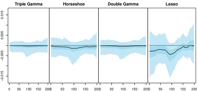
Figure 5: Posterior path against time for a constant non-significant parameter in the sparse regime.

Figure 5 shows the posterior path against time for a constant non-significant parameter, that is one for which $\theta_{ij}^{\beta}=0$ and $\beta_{ij}^{\beta}=0$ for all times, in the sparse regime. The entire set of states for the triple gamma prior can be found in Appendix C. Note that, while the zero line is contained in the 95% posterior credible interval for all priors, said interval is thinner under the triple gamma prior and the double gamma prior than under the Lasso and the Horseshoe prior. However, the light tails of the double gamma prior, as the ones of the Lasso, can over-shrink weak signals.

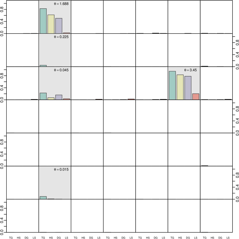
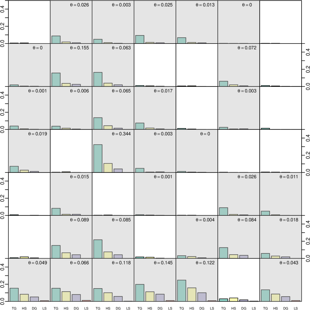
Figure 6: Posterior inclusion probability for the $\theta^{\beta}_{ij}$’s in the sparse and dense regime, under the triple gamma prior, the Horseshoe prior, the Lasso prior and the double gamma prior. The true values of the $\theta^{\beta}_{ij}$’s are reported in each cell.

The above statement becomes clearer when looking at the posterior inclusion probabilities. We calculate the posterior inclusion probabilities based on the thresholding approach introduced in Section 3.2, comparing the fully unimpeded triple gamma prior to widely used special cases. Figure 6 show the posterior inclusion probability for the variance of the innovations ($\theta^{\beta}_{ij}$’s) under four different shrinkage priors, for the sparse and the dense scenario, respectively. The cells are shaded in gray when the corresponding true state parameter is time-varying ($\theta^{\beta}_{ij}\neq 0$), while the background is white when the corresponding true state parameter is not time-varying ($\theta^{\beta}_{ij}=0$). The posterior inclusion probabilities under the triple gamma prior are consistently higher for the states for which the parameters are actually time-varying. In some cases, that heavier tails of our prior pick up signals that the other shrinkage priors are not able to capture. On the other hand, the triple gamma identifies constant parameters, effectively pulling the appropriate $\theta^{\beta}_{ij}$’s to zero.

5.4 Modeling area macroeconomic and financial variables in the Euro Area

Our application investigates a subset of the area wide model of the European Union of Fagan et al. (2005), which comprises quarterly macroeconomic data spanning from 1970 to 2017. We include 7 of the variables present in the dataset, namely real output (YER), prices (YED) , short-term interest rate (STN), investment (ITR), consumption (PCR), exchange rate (EEN) and unemployment (URX). A more detailed description of the data and the transformations performed to make the time series stationary can be found in Table 2 in Appendix D. To stay in line with the literature, e.g. Feldkircher et al. (2017), we estimate a TVP-VAR-SV model with $p=2$ lags on all endogenous variables. The hyperparameter choices are the same as in Section 5.3. As in the example with simulated data, we run the algorithm for $M=200000$ iterations, discarding the first $100000$ iterations as burn-in, and then keeping the output of one every $100$ iterations.

Figures 7 and 8 display the posterior inclusion probabilities for the means of the initial states and the innovation variances of the VAR coefficients, respectively. A few things about Figure 7 are striking. First, the posterior inclusion probabilities on the diagonal, meaning those belonging to the parameter of each equation’s own autoregressive term, appear to be those that are the highest, while off diagonal elements are more likely to be excluded. Second, the equation for the short-term interest rate is characterized by a large amount of parameters with a high inclusion probability, across all priors. Third, the first lag tends to have higher posterior inclusion probabilities than the second lag, which is in line with the literature. Finally, the triple gamma prior can be seen to often have either the largest or the smallest posterior inclusion probability compared to the other priors, which can be seen as a reflection of the high amount of prior mass placed near , as illustrated in Section 3. This BMA-like behavior yields a prior that is prone to be more absolute when it comes to inclusion decisions.

Now, we shift our focus to the posterior inclusion probabilities for the $\theta^{\beta}_{ij}$’s plotted in Figure 8. Compared to the means of the inital states, almost all inclusion probabilities are essentially zero, with virtually only the triple gamma picking up (faint) signals, in particular with respect to the equations for the financial variables in the model, namely interest rate and nominal exchange rate. This lack of variability is unsurprising, as it is well known (see, e.g., Feldkircher et al. (2017)) that stochastic volatility in a TVP-VAR model for macroeconomic variables can explain a large part of the variability in the data. Despite this, the triple gamma, thanks to its heavy tails, is still capable of picking up weak signals in the data that the other shrinkage priors we considered are not able to discern from noise.

Given that the triple gamma tends to include more time variation than the other priors, overfitting might be considered a concern. However, Figures put these fears to rest. They display the posterior median of , respectively. Here the triple gamma can be seen to be quite conservative, both in terms of which parameters to include, as well as their magnitude. In particular the medians of the $\left\lvert\sqrt{\theta}^{\beta}_{ij}\right\rvert$ are interesting, as they are closest to zero under the triple gamma prior, despite having the highest posterior inclusion probabilities among all considered priors, pointing towards the triple gamma’s ability to pick up even small signals with a higher degree of confidence than other priors.

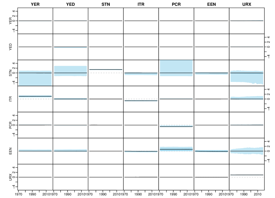
Figure 13: Each cell represents the corresponding state of the matrix , for $t=1,\ldots,T$, for the data described in Section 5.4. The solid line is the median and the shaded areas represent $50\%$ and $95\%$ posterior credible intervals.

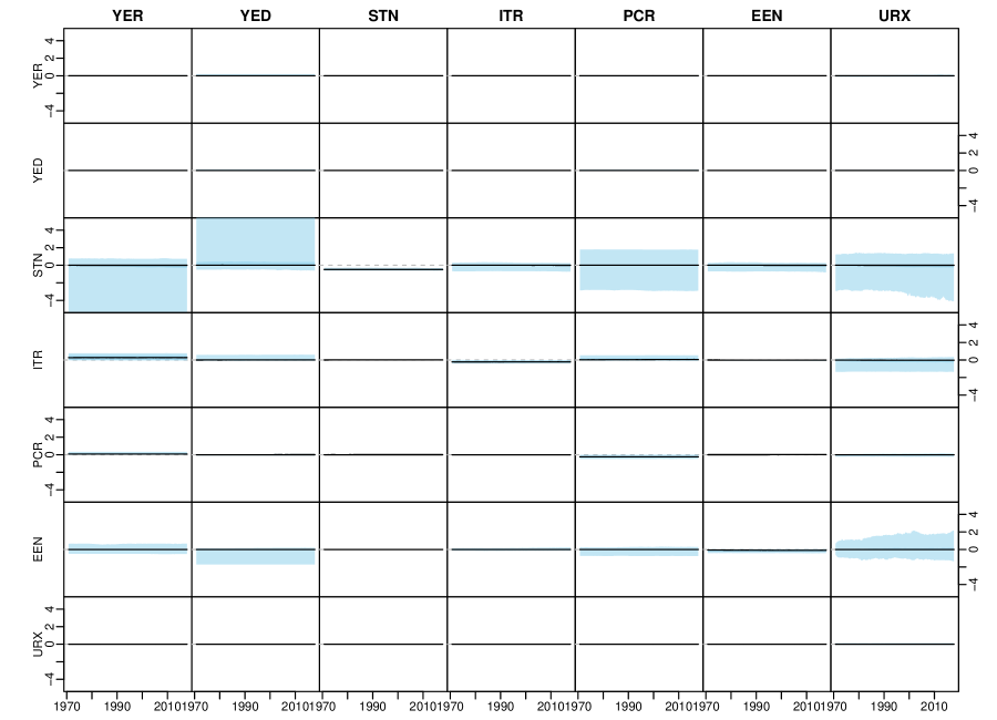
Figure 14: Each cell represents the corresponding state of the matrix , for $t=1,\ldots,T$, for the data described in section 5.4. The solid line is the median and the shaded areas represent $50\%$ and $95\%$ posterior credible intervals.

In Figures 13 and 14 in Appendix D, all the posterior paths of under the triple gamma prior are shown.

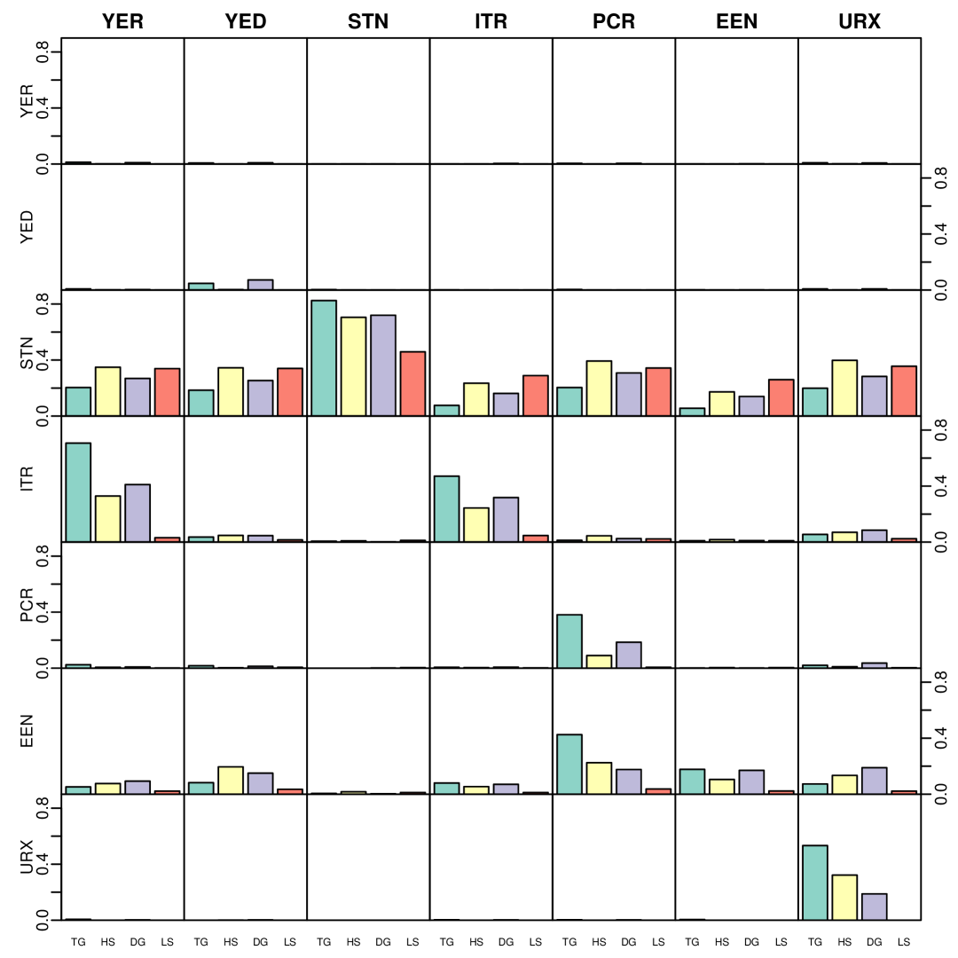
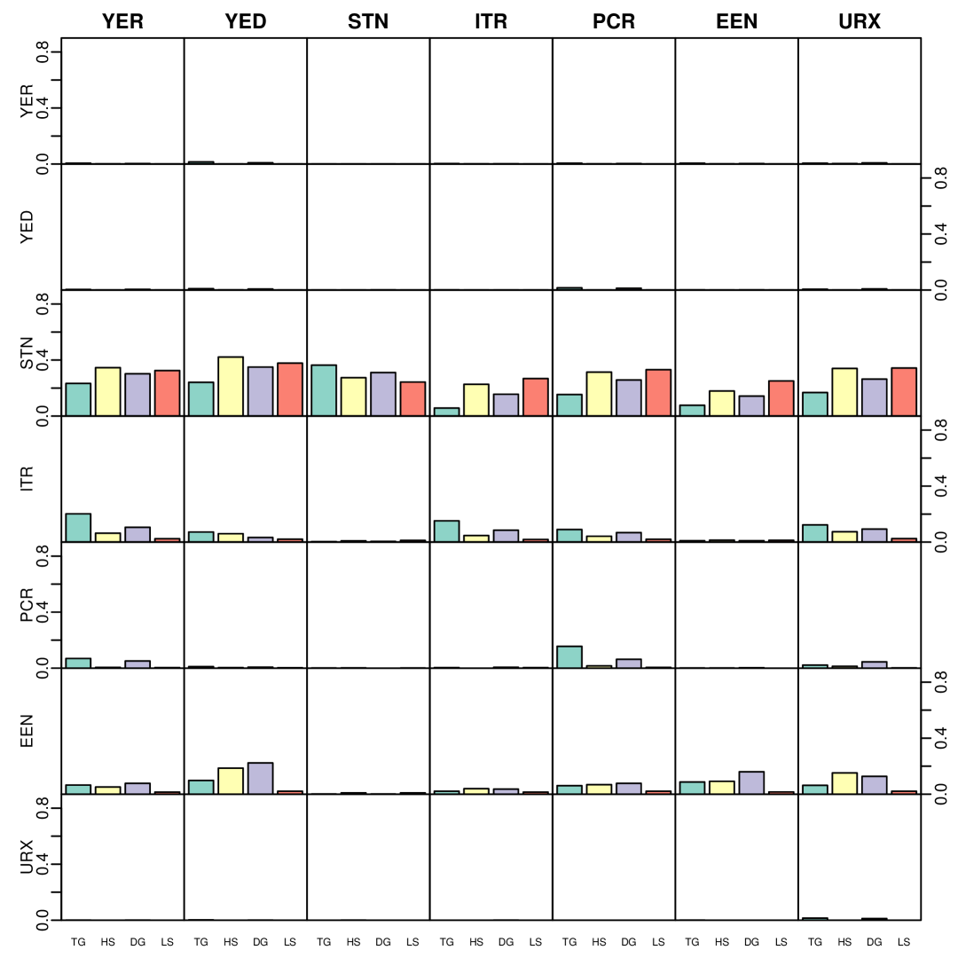
Figure 7: Posterior inclusion probability for state parameters associated with the first lag (on the left) and with the second lag (on the right), for the EA data under the triple gamma prior, the Horseshoe prior, the Lasso prior and the double gamma prior.

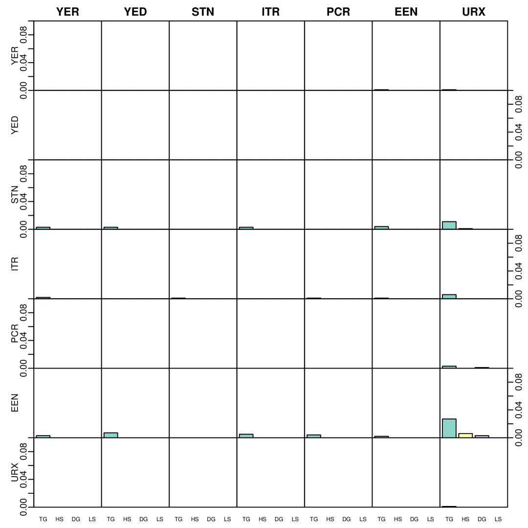
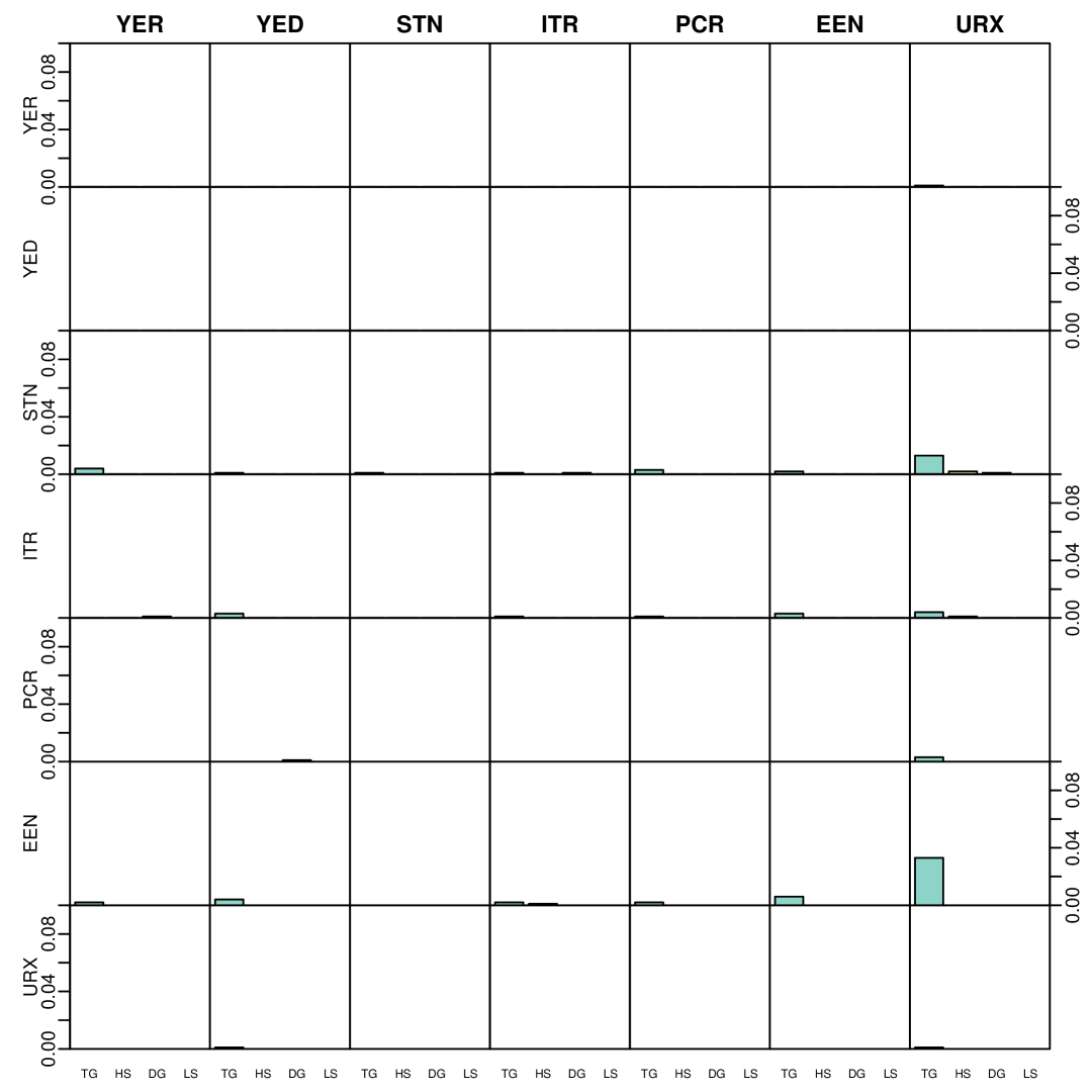
Figure 8: Posterior inclusion probability for $\theta^{\beta}_{ij}$’s associated with the first lag on the left and with the second lag on the right, for the EA data under the triple gamma prior, the Horseshoe prior, the Lasso prior and the double gamma prior.

Figure 9: Posterior median of $\beta^{\beta}_{ij}$ under the triple gamma, Horseshoe, double gamma and Lasso for the Euro area model. The vertical lines delimit the intercept, first and second lag, respectively.

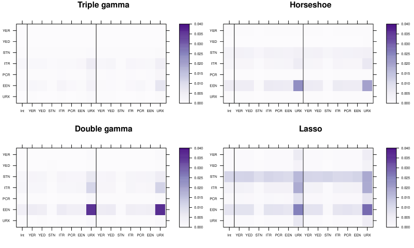
Figure 10: Posterior median of $\left\lvert\sqrt{\theta}^{\beta}_{ij}\right\rvert$ under the triple gamma, Horseshoe, double gamma and Lasso for the Euro area model. The vertical lines delimit the intercept, first and second lag, respectively

6 Conclusion

In the present paper, shrinkage for time-varying parameter (TVP) models was investigated within a Bayesian framework with the goal to automatically reduce time-varying parameters to static ones, if the model is overfitting. This goal was achieved by suggesting the triple gamma prior as a new shrinkage priors for the process variances of varying coefficients, extending previous work using spike-and-slab priors, the Bayesian Lasso, or the double gamma prior. The triple gamma prior is related to the normal-gamma-gamma prior applied for variable selection in highly structured regression models (Griffin and Brown, 2017). It contains the well-known Horseshoe prior as a special case, however it is more flexible, with two shape parameters that control concentration at zero and the tail behaviour. This leads to a BMA-type behaviour which allows not only variance shrinkage, but also variance selection.

In our application, we considered time-varying parameter VAR models with stochastic volatility. Overall, our findings suggest that the family of triple gamma priors introduced in this paper for sparse TVP models is successful in avoiding overfitting, if coefficients are, indeed, static or even insignificant. The framework developed in this paper is very general and holds the promise to be useful for introducing sparsity in other TVP and state space models in many different settings. Nevertheless, a number of extensions seem to be worth pursuing.

In particular, in ultra-sparse settings, modifications seem sensible. Currently, the hyperprior for the global shrinkage parameter of the triple gamma prior is selected in a way that it implies a uniform prior on “model size”. A generalization of Theorem 3.2 would allow to choose hyper priors that induce higher sparsity. Furthermore, in the variable selection literature, special priors such as the Horseshoe+ (Bhadra et al., 2017) were suggested for very sparse, ultra-high dimensional settings. Exploiting once more the non-centered parametrization of a state space model, it is straightforward to extend this prior to variance selection using following hierarchical representation:

$$\sqrt{\theta_{j}}|\kappa^{2}_{j},\xi^{2}_{j}\sim\mathcal{N}\left(0,\frac{2}{\kappa_{B}^{2}}\kappa^{2}_{j}\xi^{2}_{j}\right),\quad\kappa_{j}\sim t_{1},\quad\xi_{j}\sim t_{1}.$$

We leave both extensions for future research.

An important limitation of our approach is that shrinking a variance toward zero implies that a coefficient is fixed over the entire observation period of the time-series. In future research we will investigate dynamic shrinkage priors (Kalli and Griffin, 2014; Kowal et al., 2019; Ročková and McAlinn, 2019) where coefficients can be both fixed and dynamic.

The authors contributed equally to the work.

The authors declare no conflict of interest.

no

Appendix A Proofs

Proof of Theorem 2.2..

To proof Part (a), rewrite prior (6) in the following way by rescaling $\xi_{j}^{2}$ and $\kappa_{j}^{2}$:

$$\sqrt{\theta_{j}}|\tilde{\xi}_{j}^{2},\tilde{\kappa}_{j}^{2},\kappa_{B}^{2}\sim\mathcal{N}\left(0,\frac{2}{\kappa_{B}^{2}}\frac{\tilde{\xi}_{j}^{2}}{\tilde{\kappa}_{j}^{2}}\right),\quad\tilde{\xi}_{j}^{2}|a^{\xi}\sim\mathcal{G}\left(a^{\xi},a^{\xi}\right),\quad\tilde{\kappa}_{j}^{2}|c^{\xi}\sim\mathcal{G}\left(c^{\xi},c^{\xi}\right),$$ (30)

and use the fact that in (30) the random variable $\psi^{2}_{j}=\tilde{\xi}_{j}^{2}/\tilde{\kappa}_{j}^{2}$ follows the F-distribution:

$$\psi^{2}_{j}=\frac{\tilde{\xi}_{j}^{2}}{\tilde{\kappa}_{j}^{2}}\sim\frac{\mathcal{G}\left(a^{\xi},a^{\xi}\right)}{\mathcal{G}\left(c^{\xi},c^{\xi}\right)}=_{d}\mbox{\rm F}\left(2a^{\xi},2c^{\xi}\right),$$

where $p(\psi^{2}_{j})$ is given by:

$$p(\psi^{2}_{j})=\frac{1}{B(a^{\xi},c^{\xi})}\!\left(\frac{a^{\xi}}{c^{\xi}}\psi^{2}_{j}\right)^{a^{\xi}-1}\!\left(1+\frac{a^{\xi}}{c^{\xi}}\psi^{2}_{j}\right)^{-(a^{\xi}+c^{\xi})}.$$ (31)

This yields (8).

Using that $\eta_{j}=1/\psi^{2}_{j}\sim\mbox{\rm F}\left(2c^{\xi},2a^{\xi}\right)$, we obtain from (8) that

$$p(\sqrt{\theta_{j}}|\kappa^{2}_{B},a^{\xi},c^{\xi})= \frac{\sqrt{\kappa_{B}^{2}}(c^{\xi})^{c^{\xi}}}{\sqrt{4\pi}(a^{\xi})^{c^{\xi}}B(a^{\xi},c^{\xi})}\int_{0}^{\infty}\exp\left(-\frac{\theta_{j}\kappa_{B}^{2}\eta_{j}}{4}\right)\eta_{j}^{c^{\xi}-\frac{1}{2}}\left(1+\frac{c^{\xi}\eta_{j}}{a^{\xi}}\right)^{-(a^{\xi}+c^{\xi})}\text{d}\,\eta_{j}.$$

A change of variable with $y_{j}=c^{\xi}\eta_{j}/a^{\xi}$ proves Part (b):

$$p(\sqrt{\theta_{j}}|\phi^{\xi},a^{\xi},c^{\xi})= \frac{1}{\sqrt{2\pi\phi^{\xi}}B(a^{\xi},c^{\xi})}\int_{0}^{\infty}\exp\left(-\frac{\theta_{j}}{2\phi^{\xi}}y_{j}\right)y_{j}^{c^{\xi}-\frac{1}{2}}\left(1+y_{j}\right)^{-(a^{\xi}+c^{\xi})}\text{d}\,y_{j}$$

$$= \frac{\Gamma(c^{\xi}+\frac{1}{2})}{\sqrt{2\pi\phi^{\xi}}B(a^{\xi},c^{\xi})}U\left(c^{\xi}+\frac{1}{2},\frac{3}{2}-a^{\xi},\frac{\theta_{j}}{2\phi^{\xi}}\right),$$

where $\phi^{\xi}=\frac{2c^{\xi}}{\kappa_{B}^{2}a^{\xi}}$. ∎

Proof of Theorem 2.2..

Using Abramowitz and Stegun (1973, 13.5.8), we obtain for $a$ and $1<b<2$ fixed that $U\left(a,b,z\right)$ behaves for small $z$ as:

$$U\left(a,b,z\right)=\frac{\Gamma(b-1)}{\Gamma(a)}z^{1-b}+O(1).$$

Since $b=3/2-a^{\xi}$ in the expression for $p(\sqrt{\theta_{j}}|\phi^{\xi},a^{\xi},c^{\xi})$ given in (9), the condition $1<b<2$ is equivalent to $0<a^{\xi}<0.5$ and this proves Part (a):

$$p(\sqrt{\theta_{j}}|\phi^{\xi},a^{\xi},c^{\xi})=\frac{\Gamma(\frac{1}{2}-a^{\xi})}{\sqrt{\pi}(2\phi^{\xi})^{a^{\xi}}B(a^{\xi},c^{\xi})}\left(\frac{1}{\sqrt{\theta_{j}}}\right)^{1-2a^{\xi}}+O(1).$$

For $b=1$ we obtain from Abramowitz and Stegun (1973, 13.5.9) that $U\left(a,b,z\right)$ behaves for small $z$ as follows:

$$U\left(a,b,z\right)=-\frac{1}{\Gamma(a)}\left(\log z+\psi(a)\right)+O(|z\log z|),$$

where $\psi(\cdot)$ is the digamma function. Since $b=0$ is equivalent with $a^{\xi}=0.5$, this proves Part (b):

$$p(\sqrt{\theta_{j}}|\phi^{\xi},a^{\xi},c^{\xi})=\frac{1}{\sqrt{2\pi\phi^{\xi}}B(a^{\xi},c^{\xi})}\left(-\log\theta_{j}+\log(2\phi^{\xi})-\psi(c^{\xi}+{\frac{1}{2}})\right)+O(|\theta_{j}\log\theta_{j}|).$$

Using formulas 13.5.10-13.5.12 in Abramowitz and Stegun (1973), we obtain for $a$ and $b<1$ fixed that $U\left(a,b,z\right)$ behaves for small $z$ as follows:

$$U\left(a,b,z\right)=\left\{\begin{array}[]{ll}\displaystyle\frac{\Gamma(1-b)}{\Gamma(1+a-b)}+O(z^{1-b}),&0<b<1,\\[2.84526pt] \displaystyle\frac{1}{\Gamma(1+a)}+O(|z\log z|),&b=0,\\[5.69054pt] \displaystyle\frac{\Gamma(1-b)}{\Gamma(1+a-b)}+O(|z|),&b<0.\\[2.84526pt] \end{array}\right.$$

Since $O(z^{1-b})$ with $b<1$, $O(|z\log z|)$ and $O(|z|)$ converge to 0 as $z\rightarrow 0$, we obtain:

$$\lim_{z\rightarrow 0}U\left(a,b,z\right)=\frac{\Gamma(1-b)}{\Gamma(1+a-b)}.$$

This proves Part (c) as condition $b<1$ is equivalent to $a^{\xi}>0.5$:

$$\lim_{\sqrt{\theta_{j}}\rightarrow 0}p(\sqrt{\theta_{j}}|\phi^{\xi},a^{\xi},c^{\xi})=\frac{\Gamma(c^{\xi}+{\frac{1}{2}})}{\sqrt{2\pi\phi^{\xi}}B(a^{\xi},c^{\xi})}\lim_{z\rightarrow 0}U\left(c^{\xi}+{\frac{1}{2}},\frac{3}{2}-a^{\xi},z\right)=\frac{\Gamma(c^{\xi}+{\frac{1}{2}})\Gamma(a^{\xi}-\frac{1}{2})}{\sqrt{2\pi\phi^{\xi}}B(a^{\xi},c^{\xi})\Gamma(a^{\xi}+c^{\xi})}.$$

Finally, using Abramowitz and Stegun (1973, 13.1.8), we obtain as $z\rightarrow\infty$:

$$U\left(a,b,z\right)=z^{-a}\left[1+O\left(\frac{1}{z}\right)\right],\quad b<1.$$

Therefore as $\sqrt{\theta_{j}}\rightarrow\infty$

$$p(\sqrt{\theta_{j}}|\phi^{\xi},a^{\xi},c^{\xi})=\frac{\Gamma(c^{\xi}+{\frac{1}{2}})(2\phi^{\xi})^{c^{\xi}}}{\sqrt{\pi}B(a^{\xi},c^{\xi})}\left(\frac{1}{\sqrt{\theta_{j}}}\right)^{2c^{\xi}+1}\left[1+O\left(\frac{1}{\theta_{j}}\right)\right].$$

∎

Proof of Lemma 2.2..

Defining $\tilde{\psi}^{2}_{j}=\frac{a^{\xi}}{c^{\xi}}\psi^{2}_{j}$, representation (a) follows immediately from (8) and (31). Representation (b) is obtained from (30) by rescaling $\tilde{\xi}_{j}^{2}$ and $\tilde{\kappa}_{j}^{2}$. To derive representation (c), integrate (30) with respect to $\tilde{\kappa}_{j}^{2}$, using the common normal-scale mixture representation of the Student-$t$ distribution. Finally, representation (d) is obtain from (10) by rescaling. ∎

Proof of Theorem 3.2..

The equivalence of (23) and (24) follows immediately from $\phi^{\xi}=(c^{\xi}/a^{\xi})(2/\kappa_{B}^{2})\sim\mathcal{BP}\left(c^{\xi},a^{\xi}\right)$, since $2/\kappa_{B}^{2}\sim\mbox{\rm F}\left(2c^{\xi},2a^{\xi}\right)$. In addition, (24) implies that

$$\frac{\phi^{\xi}}{1+\phi^{\xi}}\sim\mathcal{B}\left(c^{\xi},a^{\xi}\right).$$

Using representations (13) and (14) of the tripe gamma prior, we can show:

$$\rho_{j}<0.5\quad\Leftrightarrow\quad\xi^{2}_{j}>1\quad\Leftrightarrow\quad\phi^{\xi}\tilde{\psi}^{2}_{j}>1\quad\Leftrightarrow\quad\frac{1}{1+\tilde{\psi}^{2}_{j}}<\frac{\phi^{\xi}}{1+\phi^{\xi}},$$

where $\tilde{\psi}^{2}_{j}\sim\mathcal{BP}\left(a^{\xi},c^{\xi}\right)$ and, consequently,

$$\frac{\tilde{\psi}^{2}_{j}}{1+\tilde{\psi}^{2}_{j}}\sim\mathcal{B}\left(a^{\xi},c^{\xi}\right)\quad\Leftrightarrow\quad\frac{1}{1+\tilde{\psi}^{2}_{j}}\sim\mathcal{B}\left(c^{\xi},a^{\xi}\right).$$

Hence, $\pi^{\xi}=\mbox{\rm Pr}(\rho_{j}<0.5)=F_{X}(Y)$, where $F_{X}$ is the cdf of a random variable $X\sim\mathcal{B}\left(c^{\xi},a^{\xi}\right)$ and the random variable $Y\sim\mathcal{B}\left(c^{\xi},a^{\xi}\right)$ arises from the same distribution. It follows immediately that $\pi^{\xi}\sim\mathcal{U}\left[0,1\right]$. ∎

Appendix B Details on the MCMC scheme

In Step (b),

$$p(a^{\xi}|\bm{z}_{-a^{\xi}},\bm{y}) \propto\left(\prod_{j=1}^{d}p(\sqrt{\theta_{j}}|\check{\kappa}_{j}^{2},\phi^{\xi})\right){p(\kappa_{B}^{2}|a^{\xi},c^{\xi})}p(a^{\xi}),$$

where $p(\kappa_{B}^{2}|a^{\xi},c^{\xi})$ is given by:

$$p(\kappa_{B}^{2}|a^{\xi},c^{\xi})=\frac{1}{2^{a^{\xi}}B(a^{\xi},c^{\xi})}\!\left(\frac{a^{\xi}}{c^{\xi}}\kappa_{B}^{2}\right)^{a^{\xi}-1}\!\left(1+\frac{a^{\xi}}{2c^{\xi}}\kappa_{B}^{2}\right)^{-(a^{\xi}+c^{\xi})}.$$

Therefore,

$$p(a^{\xi}|\bm{z}_{-a^{\xi}},\bm{y}) \propto\dfrac{2^{-da^{\xi}}}{{\Gamma(a^{\xi})}^{d}}(a^{\xi})^{d(a^{\xi}+1/2)/2}\left(\dfrac{\kappa_{B}^{2}}{c^{\xi}}\right)^{da^{\xi}/2}$$ (32)

$$\left(\prod_{j=1}^{d}\check{\kappa}_{j}^{2}\theta_{j}\right)^{a^{\xi}/2}\left(\prod_{j=1}^{d}K_{a^{\xi}-1/2}\left(\sqrt{\dfrac{\check{\kappa}_{j}^{2}\kappa_{B}^{2}a^{\xi}}{c^{\xi}}}|\sqrt{\theta_{j}}|\right)\right)\times$$

$${\frac{1}{2^{a^{\xi}}B(a^{\xi},c^{\xi})}\!\left(\frac{a^{\xi}}{c^{\xi}}\kappa_{B}^{2}\right)^{a^{\xi}-1}\!\left(1+\frac{a^{\xi}}{2c^{\xi}}\kappa_{B}^{2}\right)^{-(a^{\xi}+c^{\xi})}}$$

Hence, $\log q_{a}(a^{\xi})$ is given by (using $\Gamma(a^{\xi})=\Gamma(a^{\xi}+1)/a^{\xi}$):

$$\log q_{a}(a^{\xi}) =a^{\xi}\left(-d\log 2+\dfrac{d}{2}\log\kappa_{B}^{2}-\dfrac{d}{2}\log c^{\xi}+\dfrac{1}{2}\sum_{j=1}^{d}\log\check{\kappa}_{j}^{2}+\dfrac{1}{2}\sum_{j=1}^{d}\log\theta_{j}\right)$$ (34)

$$+\dfrac{5}{4}d\log a^{\xi}+d\dfrac{a^{\xi}}{2}\log a^{\xi}-d\log\Gamma(a^{\xi}+1)$$

$$+\sum_{j=1}^{d}\log K_{a^{\xi}-1/2}\left(\sqrt{\dfrac{\check{\kappa}_{j}^{2}\kappa_{B}^{2}a^{\xi}}{c^{\xi}}}|\sqrt{\theta_{j}}|\right)\qquad\text{(prior on $\theta_{j}$)}$$

$${-\log B(a^{\xi},c^{\xi})+a^{\xi}\left(\log a^{\xi}+\log(\frac{\kappa_{B}^{2}}{2c^{\xi}})\right)-\log a^{\xi}-(a^{\xi}+c^{\xi})\log\left(1+\frac{a^{\xi}\kappa_{B}^{2}}{2c^{\xi}}\right)\quad\text{(prior on $\kappa_{B}^{2}$)}}$$

$$+(\alpha_{a^{\xi}}-1)\log(2a^{\xi})-(\beta_{a^{\xi}}-1)\log(1-2a^{\xi})\qquad\text{(prior on $a^{\xi}$)}$$ (35)

$$+\log a^{\xi}+\log(0.5-a^{\xi})\qquad\text{(change of variable)}$$

In Step (c),

$$p(\check{\xi}_{j}^{2}|\bm{z}_{-\check{\xi}_{j}^{2}},\bm{y}) \propto p(\sqrt{\theta_{j}}|\check{\xi}^{2}_{j},\check{\kappa}^{2}_{j},\phi^{\xi})p(\check{\xi}^{2}_{j}|a^{\xi})$$ (36)

$$\propto(\check{\xi}_{j}^{2})^{-1/2}\exp\left\{-\dfrac{\check{\kappa}_{j}^{2}}{2\phi^{\xi}\check{\xi}_{j}^{2}}\theta_{j}\right\}\times(\check{\xi}_{j}^{2})^{a^{\xi}-1}\exp\left\{-\check{\xi}_{j}^{2}\right\}$$

$$=(\check{\xi}_{j}^{2})^{a^{\xi}-1/2-1}\exp\left\{-\dfrac{1}{2}\left(\dfrac{\check{\kappa}_{j}^{2}\theta_{j}}{\phi^{\xi}}\dfrac{1}{\check{\xi}_{j}^{2}}+2\check{\xi}_{j}^{2}\right)\right\},$$

which is equal to the GIG-distribution given in (25).

In Step (d),

$$p(c^{\xi}|\bm{z}_{-c^{\xi}},\bm{y}) \propto\left(\prod_{j=1}^{d}p(\sqrt{\theta_{j}}|\check{\xi}_{j}^{2},c^{\xi},\kappa_{B}^{2})\right){p(\kappa_{B}^{2}|a^{\xi},c^{\xi})}p(c^{\xi})$$ (37)

$$\propto\left(\prod_{j=1}^{d}\frac{\Gamma(\frac{2c^{\xi}+1}{2})}{\Gamma(\frac{2c^{\xi}}{2})\left(2c^{\xi}\pi\frac{2\check{\xi}^{2}_{j}}{\kappa_{B}^{2}a^{\xi}}\right)^{1/2}}\left(1+\frac{1}{2c^{\xi}}\frac{\theta_{j}}{\left(\frac{2\check{\xi}^{2}_{j}}{\kappa_{B}^{2}a^{\xi}}\right)}\right)^{-\frac{2c^{\xi}+1}{2}}\right)\times$$

$${\frac{1}{2^{a^{\xi}}B(a^{\xi},c^{\xi})}\!\left(\frac{a^{\xi}}{c^{\xi}}\kappa_{B}^{2}\right)^{a^{\xi}-1}\!\left(1+\frac{a^{\xi}}{2c^{\xi}}\kappa_{B}^{2}\right)^{-(a^{\xi}+c^{\xi})}}$$

Hence, $\log q_{c}(c^{\xi})$ is given by (using $\Gamma(c^{\xi})=\Gamma(c^{\xi}+1)/c^{\xi}$):

$$\log q_{c}(c^{\xi}) =d\log\Gamma(c^{\xi}+0.5)-d\log\Gamma(c^{\xi}+1)+\dfrac{d}{2}\log c^{\xi}$$ (38)

$$-(c^{\xi}+0.5)\left(\sum_{j=1}^{d}\log(4c^{\xi}\check{\xi}_{j}^{2}+\theta_{j}\kappa_{B}^{2}a^{\xi})-\sum_{j=1}^{d}\log(4c^{\xi}\check{\xi}_{j}^{2})\right)\qquad\text{(prior on $\theta_{j}$)}$$

$${-\log B(a^{\xi},c^{\xi})-(a^{\xi}-1)\log c^{\xi}-(a^{\xi}+c^{\xi})\log\left(1+\frac{a^{\xi}\kappa_{B}^{2}}{2c^{\xi}}\right)\quad\text{(prior on $\kappa_{B}^{2}$)}}$$

$$+(\alpha_{c^{\xi}}-1)\log(2c^{\xi})+(\beta_{c^{\xi}}-1)(1-2c^{\xi})\qquad\text{(prior on $c^{\xi}$)}$$

$$+\log c^{\xi}+\log(0.5-c^{\xi})\qquad\text{(change of variable)}$$ (39)

In Step (e),

$$p(\check{\kappa}_{j}^{2}|\bm{z}_{-\check{\kappa}_{j}^{2}},\bm{y}) \propto p(\sqrt{\theta_{j}}|\check{\xi}^{2}_{j},\check{\kappa}^{2}_{j},\phi^{\xi})p(\check{\kappa}^{2}_{j}|c^{\xi})$$ (40)

$$\propto(\check{\kappa}_{j}^{2})^{1/2}\exp\left\{-\dfrac{\check{\kappa}_{j}^{2}}{2\phi^{\xi}\check{\xi}_{j}^{2}}\theta_{j}\right\}\times(\check{\kappa}_{j}^{2})^{c^{\xi}-1}\exp\left\{-\check{\kappa}_{j}^{2}\right\}$$

$$=(\check{\kappa}_{j}^{2})^{1/2+c^{\xi}-1}\exp\left\{-\check{\kappa}_{j}^{2}\left(\dfrac{\theta_{j}}{2\phi^{\xi}\check{\xi}_{j}^{2}}+1\right)\right\},$$

which is equal to the gamma distribution given in (26).

In Step (f), $p(d_{2}|\bm{z}_{-d_{2}},\bm{y})$ is equal to following gamma distribution:

$$p(d_{2}|\bm{z}_{-d_{2}},\bm{y}) \propto p(\kappa_{B}^{2}|d_{2})p(d_{2}|a^{\xi},c^{\xi})$$ (41)

$$\propto(d_{2})^{a^{\xi}}\exp\left\{-d_{2}\kappa_{B}^{2}\right\}(d_{2})^{c^{\xi}-1}\exp\left\{-d_{2}\dfrac{2c^{\xi}}{a^{\xi}}\right\}$$

$$=(d_{2})^{a^{\xi}+c^{\xi}-1}\exp\left\{-d_{2}\left(\kappa_{B}^{2}+\dfrac{2c^{\xi}}{a^{\xi}}\right)\right\},$$

and

$$p(\kappa_{B}^{2}|\bm{z}_{-\kappa_{B}^{2}},\bm{y}) \propto\prod_{j=1}^{d}p(\sqrt{\theta_{j}}|\check{\xi}^{2}_{j},\check{\kappa}^{2}_{j},\phi^{\xi})p(\kappa_{B}^{2}|d_{2})$$ (42)

$$\propto(\kappa_{B}^{2})^{d/2}\exp\left\{-\dfrac{\kappa_{B}^{2}a^{\xi}}{4c^{\xi}}\sum_{j=1}^{d}\dfrac{\check{\kappa}_{j}^{2}}{\check{\xi}_{j}^{2}}\theta_{j}\right\}\times{(\kappa_{B}^{2})^{a^{\xi}-1}}\exp\left\{-d_{2}\kappa_{B}^{2}\right\}$$

$$={(\kappa_{B}^{2})^{d/2+a^{\xi}-1}}\exp\left\{-\kappa_{B}^{2}\left(\dfrac{a^{\xi}}{4c^{\xi}}\sum_{j=1}^{d}\dfrac{\check{\kappa}_{j}^{2}}{\check{\xi}_{j}^{2}}\theta_{j}+d_{2}\right)\right\}$$

which is equal to the gamma distribution given in (27).

For a symmetric triple gamma prior, where $a^{\xi}=c^{\xi}$, Step (b) is modified in the following way, if Step (d) is dropped:

$$q_{a}(a^{\xi})=p(a^{\xi}|\bm{z}_{-a^{\xi}},\bm{y}){\prod_{j=1}^{d}p(\check{\kappa}_{j}^{2}|c^{\xi}=a^{\xi})}\propto p(a^{\xi}|\bm{z}_{-a^{\xi}},\bm{y}){\frac{1}{\Gamma(a^{\xi})^{d}}\left(\prod_{j=1}^{d}\check{\kappa}_{j}^{2}\right)^{a^{\xi}}},$$ (43)

where $p(a^{\xi}|\bm{z}_{-a^{\xi}},\bm{y})$ is given by (32). If Step (b) is dropped, then Step (d) is modified in the following way:

$$q_{c}(c^{\xi})=p(c^{\xi}|\bm{z}_{-c^{\xi}},\bm{y}){\prod_{j=1}^{d}p(\check{\xi}_{j}^{2}|a^{\xi}=c^{\xi})}\propto p(c^{\xi}|\bm{z}_{-c^{\xi}},\bm{y}){\frac{1}{\Gamma(c^{\xi})^{d}}\left(\prod_{j=1}^{d}\check{\xi}_{j}^{2}\right)^{c^{\xi}}},$$ (44)

where $p(c^{\xi}|\bm{z}_{-c^{\xi}},\bm{y})$ is given by (37).

Appendix C Posterior paths for the simulated data

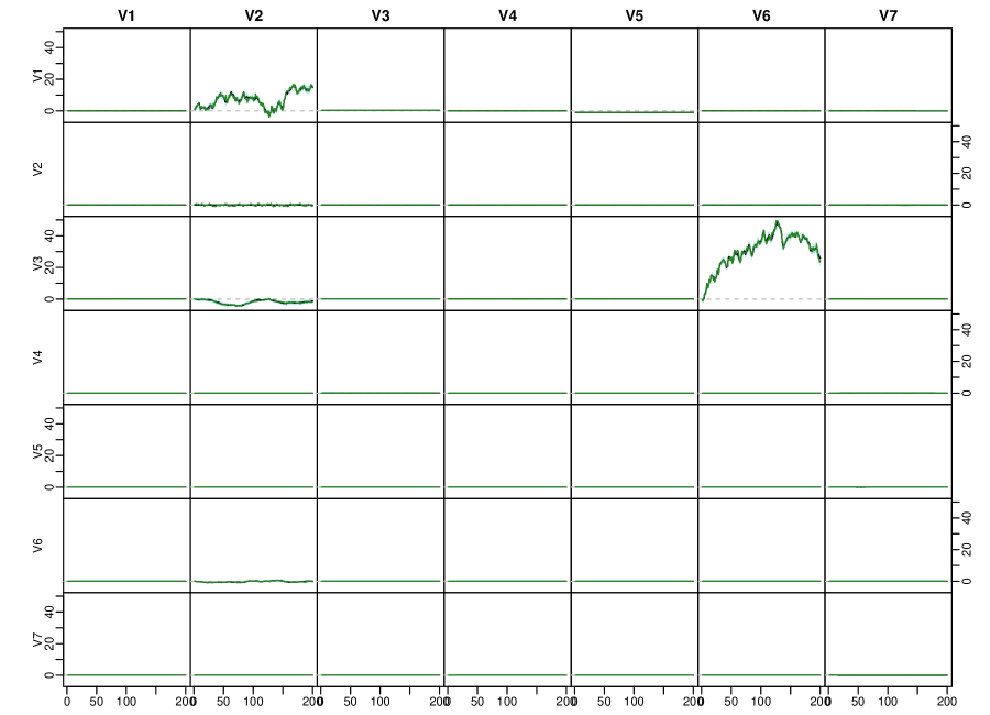
Figure 11: Each cell represents the corresponding state of the matrix , for $t=1,\ldots,T$, for the sparse regime described in Section 5.3. The solid line is the median and the shaded areas represent $50\%$ and $95\%$ posterior credible intervals.

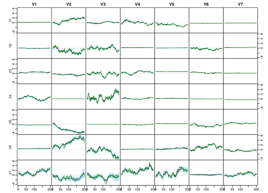
Figure 12: Each cell represents the corresponding state of the matrix , for $t=1,\ldots,T$, for the dense regime described in Section 5.3. The solid line is the median and the shaded areas represent $50\%$ and $95\%$ posterior credible intervals.

Appendix D Application

D.1 Data overview

Variable	Abbreviation	Description	Tcode
Real output	YER	Gross domestic product (GDP) at market prices in millions of Euros, chain linked volume, calendar and seasonally adjusted data, reference year 1995.	1
Prices	YED	GDP deflator, index base year 1995. Defined as the ratio of nominal and real GDP.	1
Short-term interest rate	STN	Nominal short-term interest rate, Euribor 3-month, percent per annum	2
Investment	ITR	Gross fixed capital formation in millions of Euros, chain linked volume, calendar and seasonally adjusted data, reference year 1995.	1
Consumption	PCR	Individual consumption expenditure in millions of Euros, chain linked volume, calendar and seasonally adjusted data, reference year 1995.	1
Exchange rate	EEN	Nominal effective exchange rate, Euro area-19 countries vis-à-vis the NEER-38 group of main trading partners , index base Q1 1999.	1
Unemployment	URX	Unemployment rate, percentage of civilian work force, total across age and sex, seasonally adjusted, but not working day adjusted.	2

Note: Data was retrieved from https://eabcn.org/page/area-wide-model. Tcode $=1$ indicates that differences of logs were taken, while Tcode $=2$ implies that the raw data was used.

Table 3: Data overview

D.2 Posterior paths

References

yes

Samples of the compounds …… are available from the authors.

References

• Raftery et al. (1997) Raftery, A.E.; Madigan, D.; Hoeting, J. Bayesian model averaging for linear regression models. Journal of the American Statistical Association 1997, 92, 179–191. CHECK.
• Brown et al. (2002) Brown, P.J.; Vannucci, M.; Fearn, T. Bayes model averaging with selection of regressors. Journal of the Royal Statistical Society, Ser. B 2002, 64, 519–536.
• Cottet et al. (2008) Cottet, R.; Kohn, R.J.; Nott, D.J. Variable selection and model averaging in semiparametric overdispersed generalized linear models. Journal of the American Statistical Association 2008, 103, 661–671.
• Koop and Potter (2004) Koop, G.; Potter, S.M. Forecasting in dynamic factor models using Bayesian model averaging. Econometrics Journal 2004, 7, 550–565.
• Sala-i-Martin et al. (2004) Sala-i-Martin, X.X.; Doppelhofer, G.; Miller, R.I. Determinants of long-term growth: A Bayesian averaging of classical estimates (BACE) approach. The American Economic Review 2004, 94, 813–835.
• Kleijn and van Dijk (2006) Kleijn, R.; van Dijk, H.K. Bayes model averaging of cyclical decompositions in economic time series. Journal of Applied Econometrics 2006, 21, 191–212.
• Frühwirth-Schnatter and Tüchler (2008) Frühwirth-Schnatter, S.; Tüchler, R. Bayesian Parsimonious Covariance Estimation for Hierarchical Linear Mixed Models. Statistics and Computing 2008, 18, 1–13.
• Bhadra et al. (2019) Bhadra, A.; Datta, J.; Polson, N.G.; Willard, B. Lasso meets horsheshoe: A survey. arXiv.1706.10179v4 2019.
• Fahrmeir et al. (2010) Fahrmeir, L.; Kneib, T.; Konrath, S. Bayesian Regularisation in Structured Additive Regression: A Unifying Perspective on Shrinkage, Smoothing and Predictor Selection. Statistics and Computing 2010, 20, 203–219.
• Polson and Scott (2012) Polson, N.G.; Scott, J.G. Local shrinkage rules, Lévy processes, and regularized regression. Journal of the Royal Statistical Society, Ser. B 2012, 74, 287–311.
• Tibshirani (1996) Tibshirani, R. Regression shrinkage and selection via the Lasso. Journal of the Royal Statistical Society, Ser. B 1996, 58, 267–288.
• Park and Casella (2008) Park, T.; Casella, G. The Bayesian Lasso. Journal of the American Statistical Association 2008, 103, 681–686.
• Polson and Scott (2011) Polson, N.G.; Scott, J.G. Shrink Globally, Act Locally: Sparse Bayesian Regularization and Prediction. In Bayesian Statistics 9; Bernardo, J.M.; Bayarri, M.J.; Berger, J.O.; Dawid, A.P.; Heckerman, D.; Smith, A.F.M.; West, M., Eds.; Oxford University Press: Oxford (UK), 2011; pp. 501–538.
• Frühwirth-Schnatter and Wagner (2010) Frühwirth-Schnatter, S.; Wagner, H. Stochastic Model Specification Search for Gaussian and partially Non-Gaussian State Space Models. Journal of Econometrics 2010, 154, 85–100.
• Belmonte et al. (2014) Belmonte, M.A.G.; Koop, G.; Korobolis, D. Hierarchical shrinkage in time-varying parameter models. Journal of Forecasting 2014, 33, 80–94.
• Griffin and Brown (2017) Griffin, J.E.; Brown, P.J. Hierarchical Shrinkage Priors for Regression Models. Bayesian Analysis 2017, 12, 135–159.
• Bitto and Frühwirth-Schnatter (2019) Bitto, A.; Frühwirth-Schnatter, S. Achieving Shrinkage in a Time-Varying Parameter Model Framework. Journal of Econometrics 2019, 210, 75–97.
• Armagan et al. (2011) Armagan, A.; Dunson, D.B.; Clyde, M. Generalized beta mixtures of Gaussians. Advances in Neural Information Processing Systems, 2011, pp. 523–531.
• Carvalho et al. (2009) Carvalho, C.M.; Polson, N.G.; Scott, J.G. Handling sparsity via the horseshoe. Journal of Machine Learing Research W&CP 2009, 5, 73–80.
• Carvalho et al. (2010) Carvalho, C.M.; Polson, N.G.; Scott, J.G. The horseshoe estimator for sparse signals. Biometrika 2010, 97, 465–480.
• Gelman (2006) Gelman, A. Prior distributions for variance parameters in hierarchical models (Comment on Article by Browne and Draper). Bayesian Analysis 2006, 1, 515–534.
• Polson and Scott (2012) Polson, N.G.; Scott, J.G. On the half-Cauchy prior for a global scale parameter. Bayesian Analysis 2012, 7, 887–902.
• Pérez et al. (2017) Pérez, M.; Pericchi, L.R.; Ramírez, I.C. The scaled beta2 distribution as a robust prior for scales. Bayesian Analysis 2017, 12, 615–637.
• Makalic and Schmidt (2016) Makalic, E.; Schmidt, D.F. A simple sampler for the horseshoe estimator. IEEE Signal Processing Letters 2016, 23, 179–182.
• Primiceri (2005) Primiceri, G. Time varying structural vector autoregressions and monetary policy. Review of Economic Studies 2005, 72, 821–852.
• Del Negro and Primiceri (2015) Del Negro, M.; Primiceri, G.E. Time Varying Structural Vector Autoregressions and Monetary Policy: A Corrigendum. The Review of Economic Studies 2015, 82, 1342–1345.
• Nakajima (2011) Nakajima, J. Time-varying parameter VAR model with stochastic volatility: An overview of methodology and empirical applications. Monetary and Economic Studies 2011, 29, 107–142.
• Koop and Korobilis (2013) Koop, G.; Korobilis, D. Large time-varying parameter VARs. Journal of Econometrics 2013, 177, 185 – 198.
• Eisenstat et al. (2014) Eisenstat, E.; Chan, J.C.; Strachan, R.W. Stochastic Model Specification Search for Time-Varying Parameter VARs. SSRN Electronic Journal 01/2014; DOI: 10.2139/ssrn.2403560 2014.
• Chan and Eisenstat (2016) Chan, J.C.; Eisenstat, E. Bayesian model comparison for time-varying parameter VARs with stochastic volatilty. Journal of Applied Econometrics 2016, 218, 1–24.
• Feldkircher et al. (2017) Feldkircher, M.; Huber, F.; Kastner, G. Sophisticated and small versus simple and sizeable: When does it pay off to introduce drifting coefficients in Bayesian VARs. arXiv: 1711.00564 2017, ADD, ADD.
• Carriero et al. (2019) Carriero, A.; Clark, T.G.; Marcellino, M. Large Bayesian vector autoregressions with stochastic volatility and non-conjugate priors. Journal of Econometrics 2019, forthcoming, XX–XX.
• Jacquier et al. (1994) Jacquier, E.; Polson, N.G.; Rossi, P.E. Bayesian analysis of stochastic volatility models. Journal of Business & Economic Statistics 1994, 12, 371–417.
• Frühwirth-Schnatter (2004) Frühwirth-Schnatter, S. Efficient Bayesian Parameter Estimation. In State Space and Unobserved Component Models: Theory and Applications; Harvey, A.; Koopman, S.J.; Shephard, N., Eds.; Cambridge University Press: Cambridge, 2004; pp. 123–151.
• Strawderman (1971) Strawderman, W. Proper Bayes minmax estimators of the multivariate normal mean. The Annals of Statistics 1971, 42, 385–388.
• Berger (1980) Berger, J.O. A robust generalized Bayes estimator and confidence region for a multivariate normal mean. The Annals of Statistics 1980, 8, 716–761.
• van der Pas et al. (2014) van der Pas, S.; Kleijn, B.; van der Vaart, A. The horseshoe estimator: Posterior concentration around nearly black vectors. Electronic Journal of Statistics 2014, 8, 2585–2618.
• Griffin and Brown (2011) Griffin, J.E.; Brown, P.J. BAYESIAN HYPER-LASSOS WITH NON-CONVEX PENALIZATION. Australian & New Zealand Journal of Statistics 2011, 53, 423–442.
• Scheipl and Kneib (2009) Scheipl, F.; Kneib, T. Locally adaptive Bayesian p-splines with a normal-exponential-gamma prior. Computational Statistics and Data Analysis 2009, 53, 3533–3352.
• Zhang et al. (2017) Zhang, Y.; Reich, B.J.; Bondell, H.D. High dimensional linear regression via the R2-D2 shrinkage prior. Technical report, arXiv.1609.00046v2, 2017.
• Figueiredo (2003) Figueiredo, M.A.T. Adaptive sparseness for supervised learning. IEEE Transaction on Pattern Analysis and Machine Intelligence 2003, 25, 1150–1159.
• Bhadra et al. (2017) Bhadra, A.; Datta, J.; Polson, N.; Willard, B. Horseshoe regularization for feature subset selection. arXiv:1702.07400, 2017.
• Johnstone and Silverman (2004) Johnstone, I.M.; Silverman, B.W. Needles and straw in haystacks: empirical Bayes estimates of possibly sparse sequences. The Annals of Statistics 2004, 32, 1594–1649.
• Fernández et al. (2001) Fernández, C.; Ley, E.; Steel, M.F.J. Benchmark priors for Bayesian model averaging. Journal of Econometrics 2001, 100, 381–427.
• Ley and Steel (2009) Ley, E.; Steel, M.F.J. On the effect of prior assumptions in Bayesian model averaging with applications to growth regression. Journal of Applied Econometrics 2009, 24, 651–674.
• Kastner and Frühwirth-Schnatter (2014) Kastner, G.; Frühwirth-Schnatter, S. Ancillarity-sufficiency interweaving strategy (ASIS) for boosting MCMC estimation of stochastic volatility models. Computational Statistics and Data Analysis 2014, 76, 408–423.
• Kastner (2016) Kastner, G. Dealing with Stochastic Volatility in Time Series Using the R Package stochvol. Journal of Statistical Software 2016, 69, 1–30.
• Fagan et al. (2005) Fagan, G.; Henry, J.; Mestre, R. An area-wide model for the euro area. Economic Modelling 2005, 22, 39–59.
• Feldkircher et al. (2017) Feldkircher, M.; Huber, F.; Kastner, G. Sophisticated and small versus simple and sizeable: When does it pay off to introduce drifting coefficients in Bayesian VARs?, 2017, [arXiv:stat.ME/1711.00564].
• Bhadra et al. (2017) Bhadra, A.; Datta, J.; Polson, N.; Willard, B. The horseshoe$+$ estimator of ultra-sparse signals. Bayesian Analysis 2017, 12, 1105–1131.
• Kalli and Griffin (2014) Kalli, M.; Griffin, J.E. Time-varying sparsity in dynamic regression models. Journal of Econometrics 2014, 178, 779–793.
• Kowal et al. (2019) Kowal, D.; Matteson, D.S.; Ruppert, D. Dynamic shrinkage processes. Journal of the Royal Statistical Society, Ser. B 2019.
• Ročková and McAlinn (2019) Ročková, V.; McAlinn, K. Dynamic Variable Selection with Spike-and-Slab Process Priors 2019. arXiv:1708.00085.
• Abramowitz and Stegun (1973) Abramowitz, M.; Stegun, I.A., Eds. Handbook of Mathematical Functions, New York, 1973. Dover Publications.
\sampleavailability