Hybrid Kronecker Product Decomposition and Approximation

Abstract

Discovering the underlying low dimensional structure of high dimensional data has attracted a significant amount of researches recently and has shown to have a wide range of applications. As an effective dimension reduction tool, singular value decomposition is often used to analyze high dimensional matrices, which are traditionally assumed to have a low rank matrix approximation. In this paper, we propose a new approach. We assume a high dimensional matrix can be approximated by a sum of a small number of Kronecker products of matrices with potentially different configurations, named as a hybird Kronecker outer Product Approximation ($h$KoPA). It provides an extremely flexible way of dimension reduction compared to the low-rank matrix approximation. Challenges arise in estimating a $h$KoPA when the configurations of component Kronecker products are different or unknown. We propose an estimation procedure when the set of configurations are given and a joint configuration determination and component estimation procedure when the configurations are unknown. Specifically, a least squares backfitting algorithm is used when the configuration is given. When the configuration is unknown, an iterative greedy algorithm is used. Both simulation and real image examples show that the proposed algorithms have promising performances. The hybrid Kronecker product approximation may have potentially wider applications in low dimensional representation of high dimensional data.

Keywords: Configuration, Kronecker Product, High Dimensional Matrix Approximation, Information Criterion, Model Selection, Matrix Decomposition,

1 Introduction

High dimensional data often has low dimensional structure that allows significant dimension reduction and compression. In applications such as data compression, image denoising and processing, matrix completion, high dimensional matrices are often assumed to be of low rank and can be represented as a sum of several rank-one matrices (vector outer products) in a singular value decomposition (SVD) form. Eckart and Young (1936) reveals the connection between singular value decomposition and low-rank matrix approximation. Recent studies include image low-rank approximation (Freund et al., 1999), principle component analysis (Wold et al., 1987; Zou et al., 2006), factorization in high dimensional time series (Lam and Yao, 2012; Yu et al., 2016), non-negative matrix factorization (Hoyer, 2004; Cai et al., 2009), matrix factorization for community detection (Zhang and Yeung, 2012; Yang and Leskovec, 2013; Le et al., 2016), matrix completion problems (Candès and Recht, 2009; Candes and Plan, 2010; Yuan and Zhang, 2016), low rank tensor approximation (Grasedyck et al., 2013), machine learning applications (Guillamet and Vitrià, 2002; Pauca et al., 2004; Zhang et al., 2008; Sainath et al., 2013), among many others.

As an alternative to vector outer product, the Kronecker product is another way to represent a high dimensional matrix with a much fewer number of elements. The decomposition of a high dimensional matrix into the sum of several Kronecker products of identical configuration is known as Kronecker product decomposition (Van Loan and Pitsianis, 1993). Here configuration refers to the dimensions of the component matrices of the Kronecker product. The form of Kronecker product appears in many fields including signal processing, image processing and quantum physics (Werner et al., 2008; Duarte and Baraniuk, 2012; Kaye et al., 2007), where the data has an intrinsic Kronecker product structure. Cai et al. (2019) considers to model a high dimensional matrix with a sum of several Kronecker products of the same but unknown configuration. For a given configuration, the approximation using a sum of several Kronecker products can be turned into an approximation using a sum of several rank-one matrices problem after a rearrangement operation of the matrix elements (Van Loan and Pitsianis, 1993; Cai et al., 2019). The unknown configuration can be estimated by minimizing an information criterion as proposed by Cai et al. (2019).

However, it is often the case that the Kronecker outer Product (KoPA) using a single configuration requires a large number of terms to make the approximation accurate. By allowing the use of a sum of Kronecker products of different configurations, an observed high dimensional matrix (image) can be approximated more effectively using a much smaller number of parameters (elements). We note that often the observed matrix can have much more complex structure than a single Kronecker product can handle. For example, representing an image with Kronecker products of the same configuration is often not satisfactory since the configuration dimensions determine the block structure of the recovered image, similar to the pixel size of the image. A single configuration is often not possible to provide as much details as needed, as seen from the top row of Figure 10 later. Similar to the extension from low rank matrix approximation to KoPA of a single configuration, we propose to extend the Kronecker product approach to allow for multiple configurations. It is more flexible and may provide more accurate representation with a smaller number of parameters.

In this paper, we generalize the KoPA model in Cai et al. (2019) to a multi-term setting, where the observed high dimensional matrix is assumed to be generated from a sum of several Kronecker products of different configurations – we name the model hybrid KoPA ($h$KoPA). As a special case, when all the Kronecker products are vector outer products, KoPA corresponds to a low rank matrix approximation.

We consider two problems in this paper. We first propose a procedure to estimate a $h$KoPA with a set of known configurations. The procedure is based on an iterative backfitting algorithm with the basic operation being finding the least squares solution of a single Kronecker product of a given configuration to a given matrix. This operation can be obtained through a rearrangement operation and a SVD estimation. Next, we consider the problem of determining the configurations in a $h$KoPA for a given observed matrix. As exploiting the space of all possible configuration combinations is computationally expensive, we propose an iterative greedy algorithm similar to the boosting algorithm (Freund et al., 1999). In each iteration, a single Kronecker product term is added to the model by fitting the residual matrix from the previous iteration. The configuration of the added Kronecker product is determined using the procedure proposed in Cai et al. (2019). This algorithm efficiently fits a $h$KoPA model with a potentially sub-optimal solution as a compromise between computation and accuracy.

The rest of the paper is organized as follows. The $h$KoPA model is introduced and discussed in Section 2, with a set of identifiability assumptions. In Section 3, we provide the details of the iterative backfitting estimation procedure for the model with known configurations and the greed algorithm to fit a $h$KoPA with unknown configurations. Section 4 demonstrates the performance of the proposed procedures with a simulation study and a real image example. Section 5 concludes.

Notations: For a matrix $\bm{M}$, $\|\bm{M}\|_{F}:=\sqrt{\mathrm{tr}(\bm{M}\bm{M}^{T})}$ stands for its Frobenius norm and $\|\bm{M}\|_{S}$ stands for its spectral norm, which corresponds to the largest singular value of $\bm{M}$.

2 Hybrid Kronecker Product Model

For simplicity, in this paper we assume the dimensions $(P,Q)$ of the observed matrix are of powers of 2. As a consequence, all the component matrices in $h$KoPA are also of powers of 2. The model and procedures apply to all other cases of $(P,Q)$ for which the dimensions of the component matrices in $h$KoPA are then the factors of $P$ and $Q$, with more complex notations.

In a $K$-term $h$KoPA model, we assume that the observed $2^{M}\times 2^{N}$ matrix $\bm{Y}$ is generated from the sum of $K$ Kronecker products of configurations $(m_{k},n_{k})$,

$$\bm{Y}=\sum_{k=1}^{K}\lambda_{k}\bm{A}_{k}\otimes\bm{B}_{k}+\sigma\bm{E},$$ (1)

where the matrix $\bm{A}_{k}$ is of dimension $2^{m_{k}}\times 2^{n_{k}}$, the matrix $\bm{B}_{k}$ is of dimensions $2^{M-m_{k}}\times 2^{N-n_{k}}$, for $k=1,\dots,K$. The matrix $\bm{E}$ is the noise matrix with i.i.d. standard Gaussian entities. The operation $\otimes$ denotes the Kronecker product such that for any two matrices $\bm{A}\in\mathbb{R}^{2^{m}\times 2^{n}}$ and $\bm{B}\in\mathbb{R}^{2^{M-m}\times 2^{N-n}}$, $\bm{A}\otimes\bm{B}$ is a $2^{M}\times 2^{N}$ block matrix defined by

$$\bm{A}\otimes\bm{B}=\begin{bmatrix}a_{1,1}\bm{B}&a_{1,2}\bm{B}&\cdots&a_{1,2^{n}}\bm{B}\\ a_{2,1}\bm{B}&a_{2,2}\bm{B}&\cdots&a_{2,2^{n}}\bm{B}\\ \vdots&\vdots&\ddots&\vdots\\ a_{2^{m},1}\bm{B}&a_{2^{m},2}\bm{B}&\cdots&a_{2^{m},2^{n}}\bm{B}\end{bmatrix},$$

where $a_{i,j}$ is the $(i,j)$-th element of $\bm{A}$. To better present the block structure of the Kronecker product, for any $2^{M}\times 2^{N}$ matrix $\bm{M}$, we denote $\bm{M}_{i,j}^{p,q}$ as the $(i,j)$-th $2^{p}\times 2^{q}$ block of $\bm{M}$ such that $[\bm{A}\otimes\bm{B}]_{i,j}^{M-m,N-n}=a_{i,j}\bm{B}$. We denote the dimensions $(m,n,M-m,N-n)$ as the configuration of the Kroneker product $\bm{A}\otimes\bm{B}$. When $(M,N)$ are fixed, we simplify the configuration notation as $(m,n)$.

We denote the configuration of the $h$KoPA model in (1) as the collection of configurations ${\cal C}=\{(m_{k},n_{k})\}_{k=1}^{K}$. The Kronecker product components in (1) are allowed to have different configurations $(m_{k},n_{k})$. When the model configuration ${\cal C}$ is known, we need to estimate the component matrices $\bm{A}_{k}$ and $\bm{B}_{k}$, for $k=1,\ldots,K$ in model (1). When the configuration ${\cal C}$ is unknown, the estimation of model (1) requires the determination of the configuration ${\cal C}$ as well, resulting in a configuration determination problem in addition to the estimation problem.

Some existing researches on Kronecker product structured data can be viewed as the special cases of model (1). When $K=1$ and the configuration is unknown, model (1) reduces to the single-term KoPA model investigated in Cai et al. (2019). When the configurations of the $K$ Kronecker products are known and equal such that $(m_{1},n_{1})=(m_{2},n_{2})=\dots=(m_{K},n_{K})$, an estimation of model (1) is provided by the Kronecker product decomposition approximation (Van Loan and Pitsianis, 1993).

First we note that model (1) is not identifiable. Similar to the single-term KoPA model in Cai et al. (2019), Assumption 1 below is imposed such that $\bm{A}_{k}$ and $\bm{B}_{k}$ are normalized and the Kronecker products are in decreasing order of the coefficient $\lambda_{k}$ such that given the values of the $K$ Kronecker products, $\lambda_{k}$, $\bm{A}_{k}$ and $\bm{B}_{k}$ can be uniquely determined with an exception for the sign changes of $\bm{A}_{k}$ and $\bm{B}_{k}$.

Assumption 1 (Identifiability Condition 1).

We assume

$$\|\bm{A}_{k}\|_{F}=\|\bm{B}_{k}\|_{F}=1,\text{ for }k=1,\dots,K,$$

and $\lambda_{1}\geqslant\lambda_{2}\geqslant\cdots\geqslant\lambda_{K}>0$.

Notice that if a matrix $\bm{A}_{1}$ of dimension $2^{m_{1}}\times 2^{n_{1}}$ is smaller than a matrix $A_{2}$ of dimension $2^{m_{2}}\times 2^{n_{2}}$ in that $m_{1}\leqslant m_{2},\ n_{1}\leqslant n_{2}$, then for any $2^{m_{2}-m_{1}}\times 2^{n_{2}-n_{1}}$ matrix $\bm{C}$, we have

$$\lambda_{1}\bm{A}_{1}\otimes(\bm{B}_{1}+\lambda_{2}\bm{C}\otimes\bm{B}_{2})+\lambda_{2}(\bm{A}_{2}-\lambda_{1}\bm{A}_{1}\otimes\bm{C})\otimes\bm{B}_{2}=\lambda_{1}\bm{A}_{1}\otimes\bm{B}_{1}+\lambda_{2}\bm{A}_{2}\otimes\bm{B}_{2},$$ (2)

for any $\bm{B}_{1}$ of dimension $2^{M-m_{1}}\times 2^{N-n_{1}}$, and $\bm{B}_{2}$ of dimension $2^{M-m_{2}}\times 2^{N-n_{2}}$. Therefore, additional identifiability condition is needed to be imposed to $\bm{A}_{k}$ and $\bm{A}_{l}$ when $m_{k}\leqslant m_{l}$ and $n_{k}\leqslant n_{l}$ as shown in the following Assumption 2.

Assumption 2 (Identifiability Condition 2).

For any $0\leq k,l\leq K$ such that $m_{k}\leqslant m_{l}$ and $n_{k}\leqslant n_{l}$, we assume

$$\mathrm{tr}\left[\bm{A}_{l}(\bm{A}_{k}\otimes\bm{1}_{i,j}^{m_{l}-m_{k},n_{l}-n_{k}})^{T}\right]=0,$$

for all $1\leq i\leq 2^{m_{l}-m_{k}}$ and $1\leq j\leq 2^{n_{l}-n_{k}}$, where $\bm{1}_{i,j}^{m_{l}-m_{k},n_{l}-n_{k}}$ denotes the $2^{m_{l}-m_{k}}\times 2^{n_{l}-n_{k}}$ matrix whose $(i,j)$-th element is 1 with all other elements being 0. Furthermore, if $m_{k}=m_{l}$ and $n_{k}=n_{l}$, we assume

$$\mathrm{tr}[\bm{A}_{l}\bm{A}_{k}^{T}]=\mathrm{tr}[\bm{B}_{l}\bm{B}_{k}^{T}]=0.$$

Assumption 2 is an orthogonal assumption on $\bm{A}_{k}$ and $\bm{A}_{l}$ when both dimensions of $\bm{A}_{k}$ are less than or equal to the ones of $\bm{A}_{l}$. If $\bm{A}_{k}$ and $\bm{A}_{l}$ do not satisfy the condition in Assumption 2, one can always perform an orthogonalization operation by finding a $2^{m_{l}-m_{k}}\times 2^{n_{l}-n_{k}}$ non-zero matrix $\bm{C}$, whose $(i,j)$-th element is given by

$$[\bm{C}]_{i,j}=\mathrm{tr}\left[\bm{A}_{l}(\bm{A}_{k}\otimes\bm{1}_{i,j}^{m_{l}-m_{k},n_{l}-n_{k}})^{T}\right],$$ (3)

such that Assumption 2 is satisfied for $\bm{A}_{k}$ and $\bm{A}^{*}_{l}=(\bm{A}_{l}-\bm{A}_{k}\otimes\bm{C})/\|\bm{A}_{l}-\bm{A}_{k}\otimes\bm{C}\|_{F}$. Note that $\bm{C}$ in (3) is the least squares solution of $\min\|\bm{A}_{l}-\bm{A}_{k}\otimes\bm{C}\|_{F}^{2}$. The procedure of orthogonalizing $\bm{A}_{k}$ and $\bm{A}_{l}$ can be generalized to multiple terms through the Gram-Schmidt process depicted in Figure 1. Note that the identifiability Assumption 2 can be replaced with the same condition on the $\bm{B}$s, but there is no need to impose the condition on both $\bm{A}$’s and $\bm{B}$’s.

Figure 1: Gram-Schmidt Process for $h$KoPA Model • Let $(i_{1},\dots,i_{K})$ be a shuffle of the set $\{1,\dots,K\}$ such that 1. $m_{i_{j}}\leqslant m_{i_{k}}$ for all $j\leqslant k$, 2. $n_{i_{j}}\leqslant n_{i_{k}}$ for all $j\leqslant k$ such that $m_{i_{j}}=m_{i_{k}}$. • Set $\bm{A}_{i_{1}}^{*}=\bm{A}_{i_{1}}$, $\bm{B}_{i_{1}}^{*}=\bm{B}_{i_{1}}$ and $\lambda_{i_{1}}^{*}=\lambda_{i_{1}}$. • For $j=2,\dots,K$, – Let $\Omega_{j}=\{k<j:m_{k}\leqslant m_{j},n_{k}\leqslant n_{j}\}$. – Fit the following lease square problem $$\min_{\bm{C}_{k}^{j}\in\mathbb{R}^{2^{m_{i_{j}}-m_{i_{k}}}\times 2^{n_{i_{j}}-n_{i_{k}}}}}\|\bm{A}_{i_{j}}-\sum_{k\in\Omega_{j}}\bm{A}_{i_{k}}^{*}\otimes\bm{C}_{k}^{j}\|_{F}^{2},$$ and denote the solution as $\hat{\bm{C}}_{k}^{j}$ for $k\in\Omega_{j}$. – Set $\displaystyle\bm{A}_{i_{j}}^{*}$ $\displaystyle=(\bm{A}_{i_{j}}-\sum_{k\in\Omega_{j}}\bm{A}_{i_{k}}^{*}\otimes\hat{\bm{C}_{k}}^{j})/\|\bm{A}_{i_{j}}-\sum_{k\in\Omega_{j}}\bm{A}_{i_{k}}^{*}\otimes\hat{\bm{C}_{k}}^{j}\|_{F},$ $\displaystyle\lambda_{i_{j}}^{*}$ $\displaystyle=\lambda_{i_{j}}\|\bm{A}_{i_{j}}-\sum_{k\in\Omega_{j}}\bm{A}_{i_{k}}^{*}\otimes\hat{\bm{C}_{k}}^{j}\|_{F},$ $\displaystyle\bm{B}_{i_{j}}^{*}$ $\displaystyle=\bm{B}_{i_{j}}.$ – For $k\in\Omega_{j}$, update $\displaystyle\bm{B}_{i_{k}}^{*}$ $\displaystyle\leftarrow\left(\bm{B}_{i_{k}}^{*}+\dfrac{\lambda_{i_{j}}}{\lambda^{*}_{i_{k}}}\hat{\bm{C}}_{k}^{j}\otimes\bm{B}_{i_{k}}^{*}\right)/\left\|\bm{B}_{i_{k}}^{*}+\dfrac{\lambda_{i_{j}}}{\lambda^{*}_{i_{k}}}\hat{\bm{C}}_{k}^{j}\otimes\bm{B}_{i_{k}}^{*}\right\|_{F},$ $\displaystyle\lambda_{i_{k}}^{*}$ $\displaystyle\leftarrow\lambda_{i_{k}}^{*}\left\|\bm{B}_{i_{k}}^{*}+\dfrac{\lambda_{i_{j}}}{\lambda^{*}_{i_{k}}}\hat{\bm{C}}_{k}^{j}\otimes\bm{B}_{i_{k}}^{*}\right\|_{F}.$ • $\lambda_{i}^{*},\bm{A}_{i}^{*},\bm{B}_{i}^{*}$, $i=1,\dots,K$, satisfy Assumptions 1 and 2.

3 Methodology

In this section, we propose the estimation procedures for fitting the $h$KoPA model in (1). Specifically, when the configurations are known, we adopt the backfitting approach (or alternating least squares approach) to fit the model. And when the configurations are unknown, we propose a greedy approach by adding one Kronecker product component at a time.

3.1 Hybrid Kronecker Product Model with Known Configurations

When the configurations $(m_{k},n_{k})$, $k=1,\dots,K$, are known, we consider the following least squares problem.

$$\min\|\bm{Y}-\sum_{k=1}^{K}\lambda_{k}\bm{A}_{k}\otimes\bm{B}_{k}\|_{F}^{2}.$$ (4)

When $K=1$, such a problem can be solved by singular value decomposition of a rearranged version of matrix $\bm{Y}$ as shown in Cai et al. (2019). Specifically, the rearrangement operation $\mathcal{R}_{m,n}[\cdot]$ reshape the $2^{M}\times 2^{N}$matrix $\bm{Y}$ to a new $2^{m+n}\times 2^{M+N-m-n}$ matrix such that

$$\mathcal{R}_{m,n}[\bm{Y}]=[\mathrm{vec}(\bm{Y}_{1,1}^{M-m,N-n}),\dots,\mathrm{vec}(\bm{Y}_{1,2^{n}}^{M-m,N-n}),\dots,\mathrm{vec}(\bm{Y}_{2^{m},1}^{M-m,N-n}),\dots,\mathrm{vec}(\bm{Y}_{2^{m},2^{n}}^{M-m,N-n})]^{T},$$

where $\bm{Y}_{i,j}^{M-m,N-n}$ stands for the $(i,j)$-th $2^{M-m}\times 2^{N-n}$ block of matrix $\bm{Y}$ and $\mathrm{vec}(\cdot)$ is the vectorization operation that flattens a matrix to a column vector. It is pointed out by Van Loan and Pitsianis (1993) and Cai et al. (2019) that the rearrangement operation can transform a Kronecker product to a vector outer product such that

$$\mathcal{R}_{m,n}[\bm{A}\otimes\bm{B}]=\mathrm{vec}(\bm{A})\mathrm{vec}(\bm{B})^{T}.$$

This can be seen from the fact that all the elements in the matrix $\bm{A}\otimes\bm{B}$ are in the form of $a_{i,j}b_{k,\ell}$, which is exactly the same as those in $\mathrm{vec}(\bm{A})\mathrm{vec}(\bm{B})^{T}$, where $a_{i,j}$ is the $(i,j)$-th element in $\bm{A}$ and $b_{k,\ell}$ is the $(k,\ell)$-th element in $\bm{B}$.

Therefore, the least squares optimization problem

$$\min\|\bm{Y}-\lambda\bm{A}\otimes\bm{B}\|_{F}^{2},$$

is equivalent to a rank-one matrix approximation problem since

$$\|\bm{Y}-\lambda\bm{A}\otimes\bm{B}\|_{F}^{2}=\|\mathcal{R}_{m,n}[\bm{Y}]-\lambda\mathrm{vec}(\bm{A})\mathrm{vec}(\bm{B})^{T}\|_{F}^{2},$$

whose solution is given by the leading component in the singular value decomposition of $\mathcal{R}_{m,n}[\bm{Y}]$ as proved by Eckart and Young (1936).

When there are multiple terms $K>1$ in the model (1), we propose to solve the optimization problem (4) through a backfitting algorithm (or alternating least squares algorithm) by iteratively estimating $\lambda_{k}$, $\bm{A}_{k}$ and $\bm{B}_{k}$ by

$$\min\|\bm{(}Y-\sum_{i\neq k}\hat{\lambda}_{i}\hat{\bm{A}}_{i}\otimes\hat{\bm{B}}_{i})-\lambda_{k}\bm{A}_{k}\otimes\bm{B}_{k}\|_{F}^{2},$$

using the rearrangement operator and SVD, with fixed $\hat{\lambda}_{i}$, $\hat{\bm{A}}_{i}$ and $\hat{\bm{B}}_{i}$ ($i\neq k$) from previous iterations.

When all configurations $\{(m_{k},n_{k})\}_{k=1}^{K}$ are distinct, the backfitting procedure for $h$KoPA is depicted in Figure 2, where $\mathrm{vec}^{-1}_{m,n}$ is the inverse of the vectorization operation that convert a column vector back to a $2^{m}\times 2^{n}$ matrix. When $r$ terms indexed by $k_{1},\dots,k_{r}$ in the $h$KoPA model have the same configuration, these terms are updated simultaneously in the backfitting algorithm by keeping the first $r$ components from the SVD of the residual matrix $\bm{E}_{k}=\bm{Y}-\sum_{i\neq k_{1},\dots,k_{r}}\hat{\lambda}_{i}\hat{\bm{A}}_{i}\otimes\hat{\bm{B}}_{i}$. We also Orthonormalize the components by the Gram-Schmidt process at the end of each backfitting round.

Since each iteration of the backfitting procedure reduces the sum of squares of residuals, the algorithm always converges, though it may land in a local optimal. Empirical experiences show that most of the time the global minimum is reached. Starting with different initial values and order of backfitting helps.

Figure 2: Backfitting Least Squares Procedure • Set $\hat{\lambda}_{1}=\hat{\lambda}_{2}=\dots=\hat{\lambda}_{K}=0$. • Repeat until convergence: – For $k=1,\dots,K$, * Let $\bm{E}_{k}=\bm{Y}-\sum_{i\neq k}\hat{\lambda}_{i}\hat{\bm{A}}_{i}\otimes\hat{\bm{B}}_{i}$. * Compute SVD of $\mathcal{R}_{m_{k},n_{k}}[\bm{E}_{k}]$ such that $$\mathcal{R}_{m_{k},n_{k}}[\bm{E}_{k}]=\sum_{j=1}^{J}s_{j}\bm{u}_{j}\bm{v}_{j}^{T},$$ where the singular values are in decreasing order such that $s_{1}\geqslant s_{2}\geqslant\dots\geqslant s_{J}$. * Update $\hat{\lambda}_{k}=s_{1}$, $\hat{\bm{A}}_{k}=\mathrm{vec}^{-1}_{m_{k},n_{k}}(\bm{u}_{1})$ and $\hat{\bm{B}}_{k}=\mathrm{vec}^{-1}_{M-m_{k},N-n_{k}}(\bm{v}_{1})$. – Orthonormalize the components by the Gram-Schmidt process in Figure 1. • Output $\{(\hat{\lambda}_{k},\hat{\bm{A}}_{k},\hat{\bm{B}}_{k})\}_{k=1}^{K}$.

3.2 Hybrid KoPA with Unknown Configurations

In this section, we consider the case when the model configuration ${\cal C}=\{(m_{k},n_{k})\}_{k=1}^{K}$ is unknown. We use a greedy method similar to boosting to obtain the approximation by iteratively adding one Kronecker product at a time, based on the residual matrix obtained from the previous iteration. Specifically, at iteration $k$, we obtain

$$\hat{\bm{E}}^{(k)}=\bm{Y}-\sum_{i=1}^{k-1}\hat{\lambda}_{i}\hat{\bm{A}}_{i}\otimes\hat{\bm{B}}_{i},$$

where $\hat{\lambda}_{i}$, $\hat{\bm{A}}_{i}$ and $\hat{\bm{B}}_{i}$ are obtained in the previous iterations, starting with $\bm{E}^{(1)}=\bm{Y}$. Then we use the single-term KoPA with unknown configuration proposed in Cai et al. (2019) to obtain

$$\min_{\lambda_{k},\bm{A}_{k},\bm{B}_{k}}\|\bm{\hat{}}{\bm{E}}^{(k)}-\lambda_{k}\bm{A}_{k}\otimes\bm{B}_{k}\|_{F}^{2},$$

where the configuration $(m_{k},n_{k})$ of $\hat{\bm{A}}_{k}$ and $\hat{\bm{B}}_{k}$ is obtained by minimizing the information criterion

$$IC_{q}(m,n)=2^{M+N}\ln\dfrac{\|\hat{\bm{E}}^{(k)}-\lambda_{k}\bm{A}_{k}\otimes\bm{B}_{k}\|_{F}^{2}}{2^{M+N}}+qp,$$ (5)

where $p=2^{m+n}+2^{M+N-m-n}$ is the number of parameters of the single-term model with configuration $(m_{k},n_{k})$ and $q$ is the penalty coefficient on model complexity. When $q=0$ the information criterion is a monotone function of the mean squared error (MSE). When $q=2$ and $q=(M+N)\ln 2$, the information criterion $IC_{q}(m,n)$ is same as Akaike information criterion (AIC) (Akaike, 1998) and Bayes information criterion (BIC) (Schwarz, 1978), correspondingly. As shown in Cai et al. (2019), in a single-term Kronecker product case, when the signal-to-noise ratio is large enough, minimizing the information criterion $IC_{q}$ in (5) produces consistent estimators of the true configuration.

The procedure is repeated until a stopping criterion is reached. The algorithm is depicted in Figure 3.

Remark: The iterative algorithm in Figure 3 is a greedy algorithm, which does not guarantee a global optimal in all configuration combinations. The output of the algorithm satisfies Assumption 1 but does not satisfy Assumption 2. However, searching the configuration space $\{(m_{k},n_{k})\}_{k=1}^{K}$ in a greedy and additive way requires less computational power. It is possible that, given the configuration $\hat{{\cal C}}=\{(\hat{m}_{k},\hat{n}_{k}),k=1,\ldots,\hat{K}\}$ obtained in the greed algorithm, a refinement step can be engaged using the algorithm proposed in Section 3.1. If more computational resources are available, the refinement can be done at the end of each iteration $k$ based on $\hat{{\cal C}}_{k}=\{(\hat{m}_{i},\hat{n}_{i}),i=1,\ldots,k\}$ obtained to obtain better partial residual matrix $\hat{\bm{E}}^{(k)}$ so the configuration determination in future iterations are more accurate.

Remark: The stopping criterion can be selected according to the objective of the study. For denoising applications, one may specify the desired level of proportion of the total variation explained by the $h$KoPA to be reached. Similarly a scree plot approach can be used. It is also possible to minimize an overall information criterion in the form of

$$IC_{q}({\cal C})=2^{M+N}\ln\dfrac{\|\hat{\bm{Y}}-\sum_{k=1}^{K}\lambda_{k}\bm{A}_{k}\otimes\bm{B}_{k}\|_{F}^{2}}{2^{M+N}}+qp,$$ (6)

where $p=\sum_{k=1}^{K}2^{m_{k}+n_{k}}+2^{M+N-m_{k}-n_{k}}$ is the total number of parameters with the configuration ${\cal C}$. For image compression applications, the information criterion can be replaced with the ratio of explained variation to the total storage size. In Section 4.2, we will illustrate a practical stopping criterion using random matrix theory.

Remark: Compared with the backfitting algorithm for known configuration problems, the iterative algorithm in Figure 3 focuses more on the configuration determination in an iterative and additive way. When the configurations are known exactly, the backfitting algorithm in Figure 2 gives more accurate estimates of the components.

Figure 3: Iterative Algorithm for $h$KoPA Estimation • Set $\hat{\bm{E}}^{(1)}=\bm{Y}$. • For $k=1,\dots,K$: – For all $(m,n)\in\mathcal{C}:=\{0,\dots,M\}\times\{0,\dots,N\}/\{(0,0),(M,N)\}$: * Do SVD for $\mathcal{R}_{m,n}[\hat{\bm{E}}^{(k)}]$ such that $$\mathcal{R}_{m,n}[\hat{\bm{E}}^{(k)}]=\sum_{j=1}^{J}s_{j}\bm{u}_{j}\bm{v}_{j}^{T}.$$ * Set $\hat{\lambda}_{k}^{(m,n)}=s_{1}$, $\hat{\bm{A}}_{k}^{(m,n)}=\mathrm{vec}^{-1}_{m,n}(\bm{u}_{1})$ and $\hat{\bm{B}}_{k}^{(m,n)}=\mathrm{vec}^{-1}_{M-m,N-n}(\bm{v}_{1})$. * Obtain $\hat{\bm{S}}_{k}^{(m,n)}=\hat{\lambda}_{k}^{(m,n)}\hat{\bm{A}}_{k}^{(m,n)}\otimes\hat{\bm{B}}_{k}^{(m,n)}$. – Obtain $(\hat{m}_{k},\hat{n}_{k})$ through $$\hat{m}_{k},\hat{n}_{k}=\operatorname*{arg\,min}_{(m,n)\in\mathcal{C}}\ 2^{M+N}\ln\dfrac{\|\hat{\bm{E}}^{(k)}-\hat{\bm{S}}_{k}^{(m,n)}\|_{F}^{2}}{2^{M+N}}+qp.$$ – Set $\hat{\lambda}_{k}=\hat{\lambda}_{k}^{(\hat{m}_{k},\hat{n}_{k})}$, $\hat{\bm{A}}_{k}=\hat{\bm{A}}_{k}^{(\hat{m}_{k},\hat{n}_{k})}$ and $\hat{\bm{B}}_{k}=\hat{\bm{B}}_{k}^{(\hat{m}_{k},\hat{n}_{k})}$. – Break if a stopping criterion is met. – Calculate $\hat{\bm{E}}^{(k+1)}=\hat{\bm{E}}^{(k)}-\hat{\bm{S}}_{k}^{(\hat{m}_{k},\hat{n}_{k})}$. • Return $\{(\hat{\lambda}_{k},\hat{\bm{A}}_{k},\hat{\bm{B}}_{k})\}_{k=1}^{\hat{K}}$, where $\hat{K}$ is the number of terms determined by the stopping criterion.

4 Empirical Examples

4.1 Simulation

In this simulation, we exam the performance of the least squares backfitting algorithm in Figure 2 for a two-term Kronecker product model and determine the factors that may affect the accuracy and convergence speed of the algorithm.

Specifically, we simulate the data $\bm{Y}$ according to

$$\bm{Y}=\lambda_{1}\bm{A}_{1}\otimes\bm{B}_{1}+\lambda_{2}\bm{A}_{2}\otimes\bm{B}_{2}+\sigma\bm{E},$$

where $\lambda_{1}=\lambda_{2}=1$ and $\bm{A}_{k}$, $\bm{B}_{k}$ ($k=1,2$) satisfy Assumption 1. Here we assume $\bm{A}_{1}$ and $\bm{A}_{2}$ are linearly independent to ensure identifiability Assumption 2, as discussed in Section 2. If they are not linearly independent, we can always apply Gram-Schmidt process to reformulate the model so $\bm{A}_{1}$ and $\bm{A}_{2}$ are linearly independent. One of the objectives of the simulation study is to see the impact of linear dependence of $\bm{B}_{1}$ and $\bm{B}_{2}$, once we control the linear dependence of $\bm{A}_{1}$ and $\bm{A}_{2}$. The shape parameters for this simulation study is set to

$$M=N=9,\quad(m_{1},n_{1})=(4,4),\quad(m_{2},n_{2})=(5,5).$$

To simulate the component matrices, we first generate $\tilde{\bm{A}}_{1}\in\mathbb{R}^{2^{m_{1}}\times 2^{n_{1}}}$ and $\tilde{\bm{A}}_{2}\in\mathbb{R}^{2^{m_{2}}\times 2^{n_{2}}}$ by normalizing corresponding i.i.d standard Gaussian random matrices. $\tilde{\bm{A}}_{1}$ and $\tilde{\bm{A}}_{2}$ are then orthogonalized in the sense that $\|\tilde{\bm{A}}_{1}\otimes\bm{C}-\tilde{\bm{A}}_{2}\|_{F}^{2}$ is minimized at $\bm{C}=0$. Orthonormal $\tilde{\bm{B}}_{1}$ and $\tilde{\bm{B}}_{2}$ are generated in a similar way. We set

$$\bm{A}_{1}=\tilde{\bm{A}}_{1},\ \bm{A}_{2}=\tilde{\bm{A}}_{2},\ \bm{B}_{1}=\dfrac{\tilde{\bm{B}}_{1}+\alpha\bm{1}\otimes\tilde{\bm{B}}_{2}}{\sqrt{1+\alpha^{2}2^{m_{2}+n_{2}-m_{1}-n_{1}}}},\ \bm{B}_{2}=\tilde{\bm{B}}_{2},$$

where $\bm{1}$ is a $2^{m_{2}-m_{1}}\times 2^{n_{2}-n_{1}}$ matrix of ones and $\alpha$ controls the linear dependency between $\bm{B}_{1}$ and $\bm{B}_{2}$.

Note that when $\alpha=0$, $\bm{B}_{1}$ and $\bm{B}_{2}$ are linearly independent. When $\alpha\rightarrow\infty$, $\bm{B}_{1}\propto\bm{1}\otimes\bm{B}_{2}$ and the model can be represented with a single term Kronecker product.

In this simulation we consider $\alpha\in\{0,0.5,1.0,1.5,2.0\}$ and $\sigma_{0}:=2^{(M+N)/2}\sigma\in\{0,0.5,1.0,1.5,2.0\}$. The benchmark setting is $\alpha=0.5$ and $\sigma_{0}=1$, under which the signal-to-noise ratio is $(\lambda_{1}^{2}+\lambda_{2}^{2})/\sigma_{0}^{2}=2$ and $50\%$ of the variation in $\bm{B}_{1}$ can be explained by $\bm{B}_{2}$.

We first examine the effect of linear dependency of $\bm{B}_{1}$ and $\bm{B}_{2}$, controlled by $\alpha$. Hence we fix $\sigma_{0}=1$ and check the performance of the backfitting algorithm under different values of $\alpha$, using the known configurations. Figure 4 shows the relative error $\hat{\bm{Y}}$ for the first 40 iterations for the five different values of $\alpha$. At $\sigma_{0}=1$, a perfect fit is expected to have an error of

$$\dfrac{E[\|\sigma\bm{E}\|_{F}]}{E[\|\bm{Y}\|_{F}]}=\dfrac{\sigma_{0}}{\sqrt{\lambda_{1}^{2}+\lambda_{2}^{2}+\sigma_{0}^{2}}}\approx 0.577.$$

under the simulation setting. It is seen from Figure 4 that the estimates tend to overfit as the final relative errors are all smaller than the expected value. This is due to the fact that the observed error term $\bm{E}$ is not orthogonal to the observed signal. However, the less $\bm{B}_{1}$ and $\bm{B}_{2}$ are linearly dependent, the less the model is overfitted.

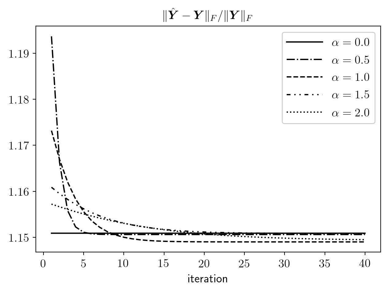
Figure 4: Fitting error against number of iterations for different $\alpha$ values, when $\sigma_{0}=1$

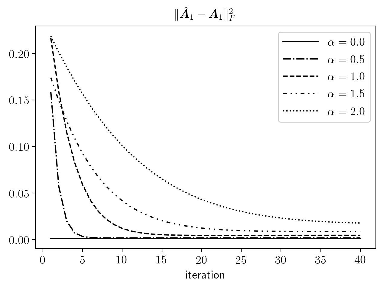
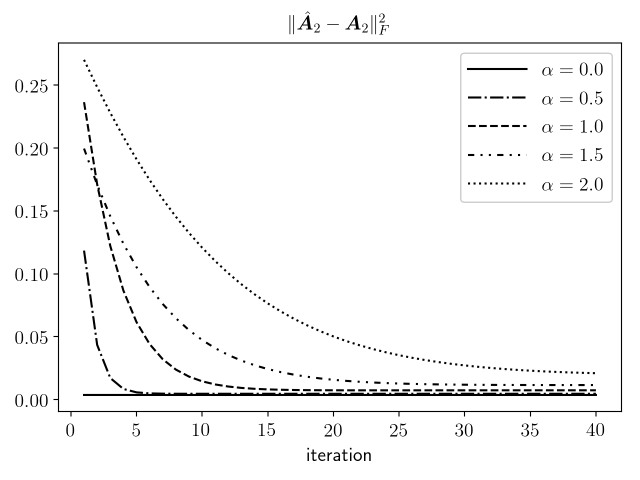
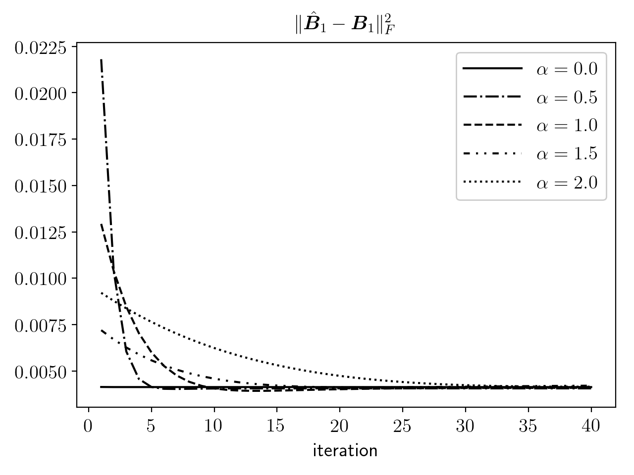
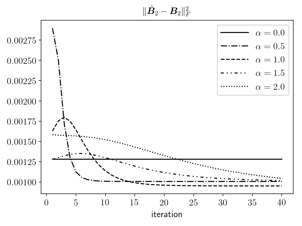
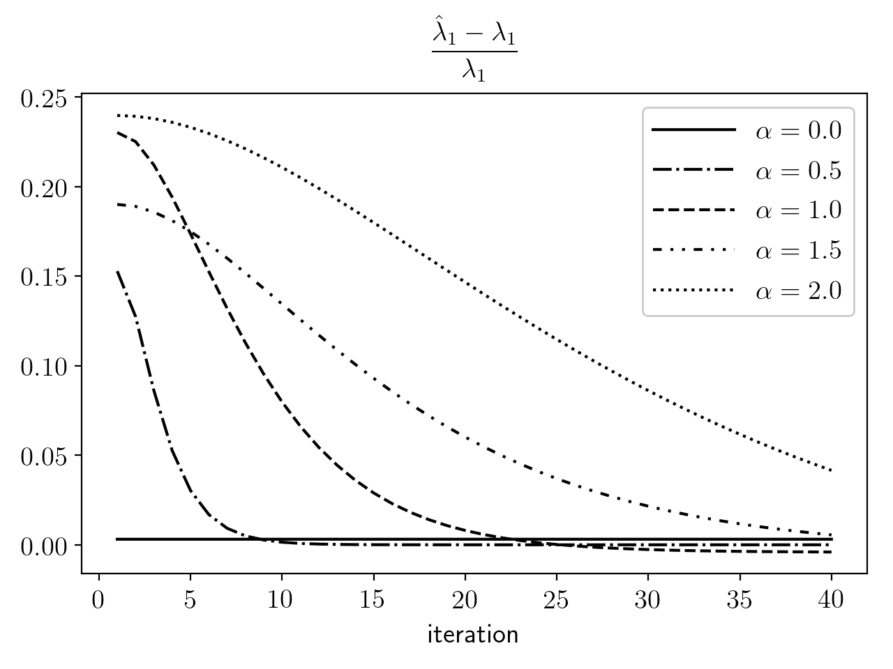
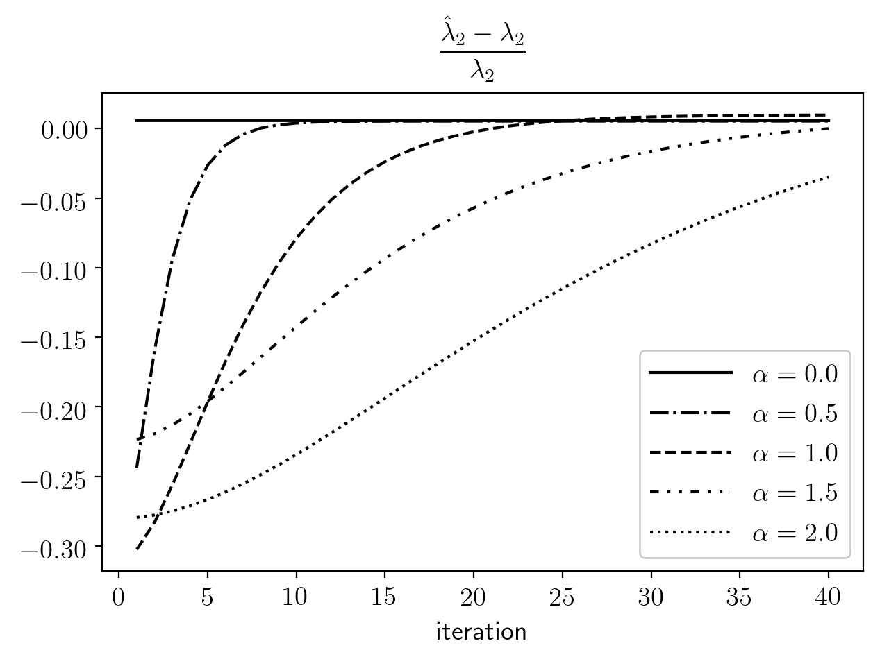
Figure 5: Errors in components against number of iterations for different $\alpha$ values.

By comparing the convergence speed of different $\alpha$ values, we notice that larger value of $\alpha$, corresponding to higher linear dependency between $\bm{B}_{1}$ and $\bm{B}_{2}$, results in a slower convergence rate. When $\bm{B}_{1}$ and $\bm{B}_{2}$ are linearly independent ($\alpha=0$), only one iteration is needed.

The errors of the estimation of the coefficients $\lambda_{1}$, $\lambda_{2}$, $\bm{A}_{1}$, $\bm{A}_{2}$, $\bm{B}_{1}$ and $\bm{B}_{2}$ plotted against the number of iterations are shown in Figure 5. For all the components, higher values of $\alpha$ result in slower convergence rates and less accurate final results.

Notice that when $\alpha>0$, the four matrices involved in the two-term model are not symmetric under the identifiability conditions using the iterative backfitting algorithm. On the one hand, $\bm{A}_{1}$ and $\bm{A}_{2}$ are enforced to be orthogonal, while $\bm{B}_{1}$ and $\bm{B}_{2}$ are not. On the other hand, the iterative backfitting algorithm fits $\bm{A}_{1}$ and $\bm{B}_{1}$ first, resulting in an overfitting for the first Kronecker product in the first iteration. Due to the asymmetry, the performance of estimating $\bm{B}_{1}$ and $\bm{B}_{2}$ is better than that of estimating $\bm{A}_{1}$ and $\bm{A}_{2}$ when $\bm{B}_{1}$ and $\bm{B}_{2}$ have linear dependency. A strong correlation between the errors in $\bm{A}_{1}$ and $\bm{A}_{2}$ is observed. We also note that the convergence rate for both $\lambda_{1}$ and $\lambda_{2}$ are slower than that for the matrices, especially for the high linear dependence cases.

Next, we examine the effect of the noise level $\sigma_{0}$. We fix $\alpha=0.5$ and consider five different values of the noise $\sigma_{0}$. The error in estimating $\bm{Y}$ is reported in Figure 6. It is seen that higher noise level $\sigma_{0}$ results in larger errors, as expected. A small difference in the convergence speed is observed as well. The algorithm converges faster when the noise level is high, but it is not as sensitive as that in the change of linear dependence level $\alpha$.

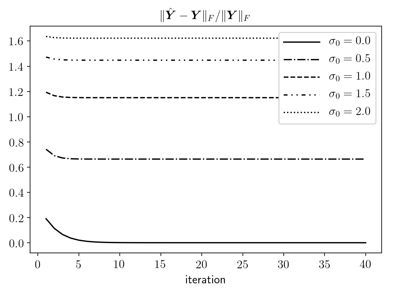
Figure 6: Fitting error against number of iterations for different $\sigma_{0}$ values

Errors for estimating the different components in the model are plotted in Figure 7 for different noise levels. The difference in convergence rates is less obvious. We also observe that the performance for estimating the smaller component matrices $\bm{A}_{1}$ and $\bm{B}_{2}$ is better than that for the larger matrices $\bm{A}_{2}$ and $\bm{B}_{1}$.

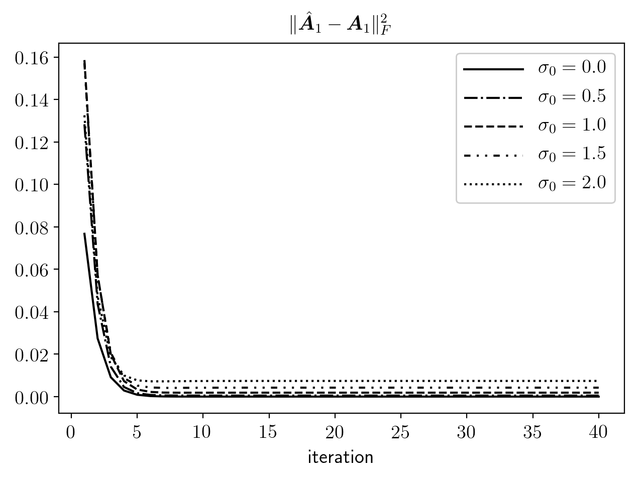
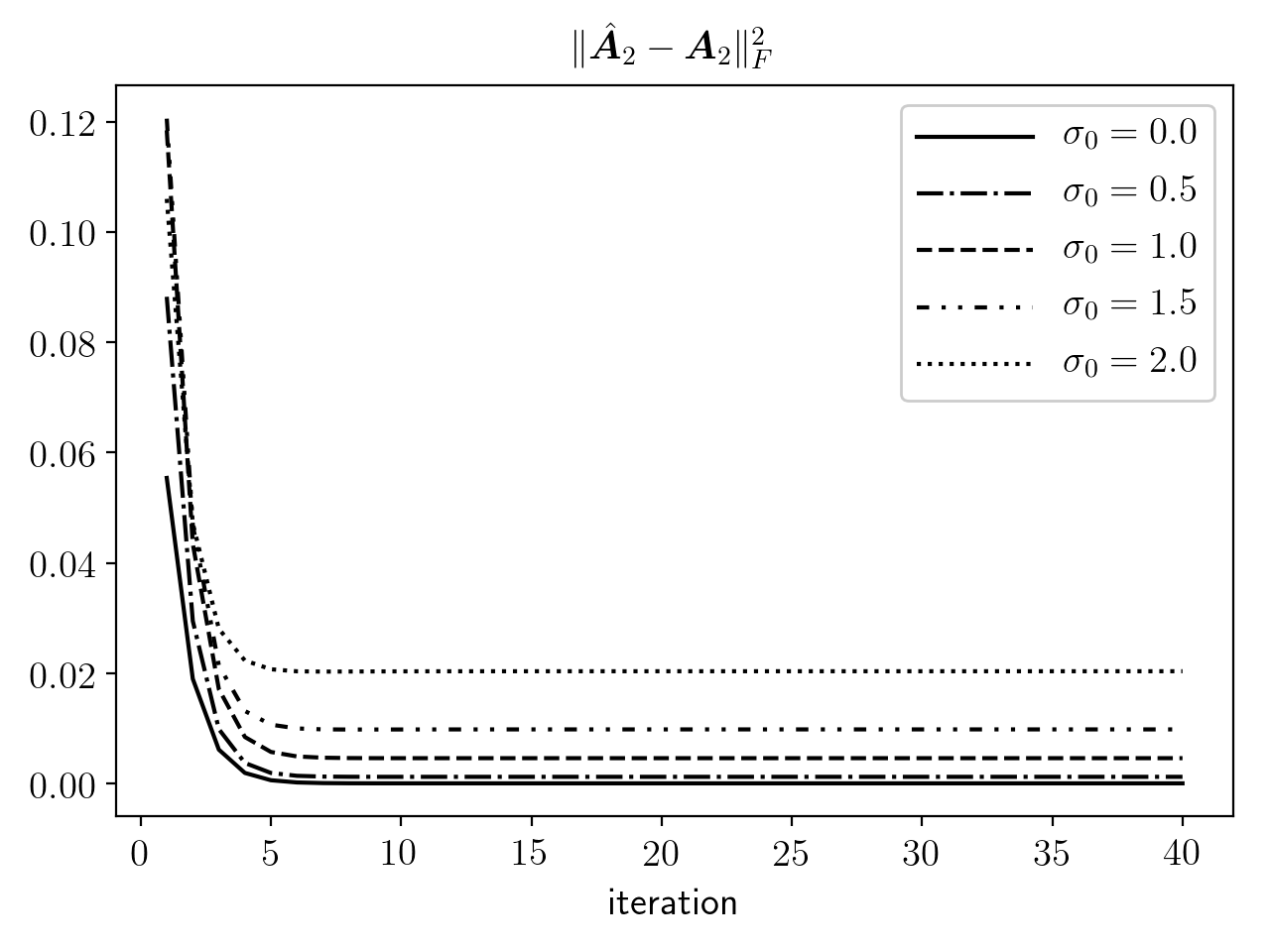
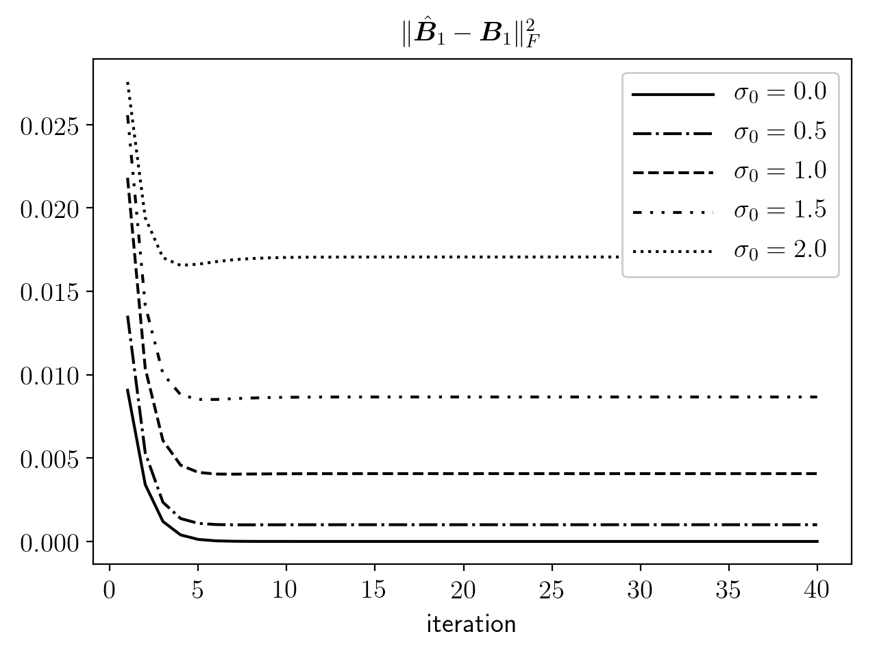
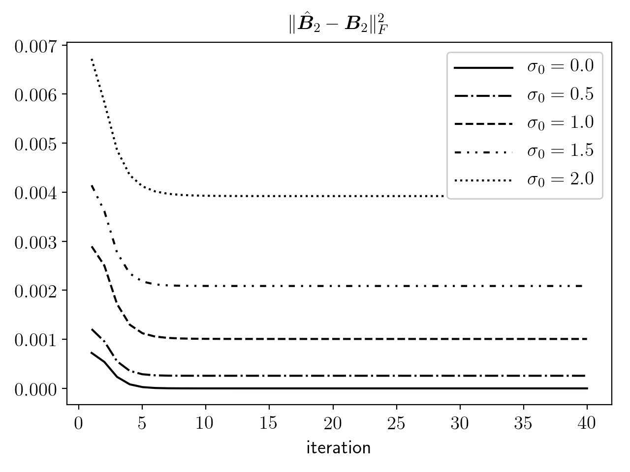
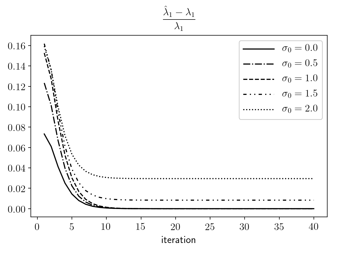
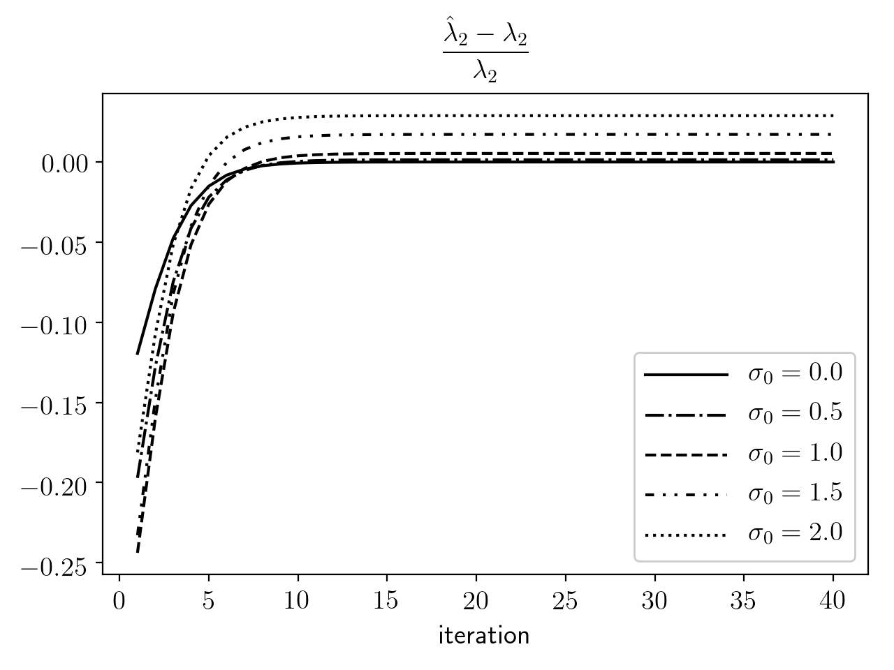
Figure 7: Errors in components against number of iterations for different $\sigma_{0}$ values.

4.2 Real image example

In this exercise, we apply the $h$KoPA to analyze the image of Lenna, which has been used widely as a benchmark image in image processing studies. The Lenna’s image shown in Figure 8 is a gray-scaled $512\times 512$ picture, which is represented by a $512\times 512$ ($M=N=9$) real matrix $\bm{Y}$. The elements of $\bm{Y}$ are real numbers between 0 and 1, where $0$ represents black and $1$ represents white. Besides the original image, in this example we also consider some artificially blurred images using

$$\bm{Y}_{\sigma}=\bm{Y}+\sigma\bm{E},$$

where $\bm{E}$ is a matrix of i.i.d. standard Gaussian random variables and $\sigma$ denotes the noise level.

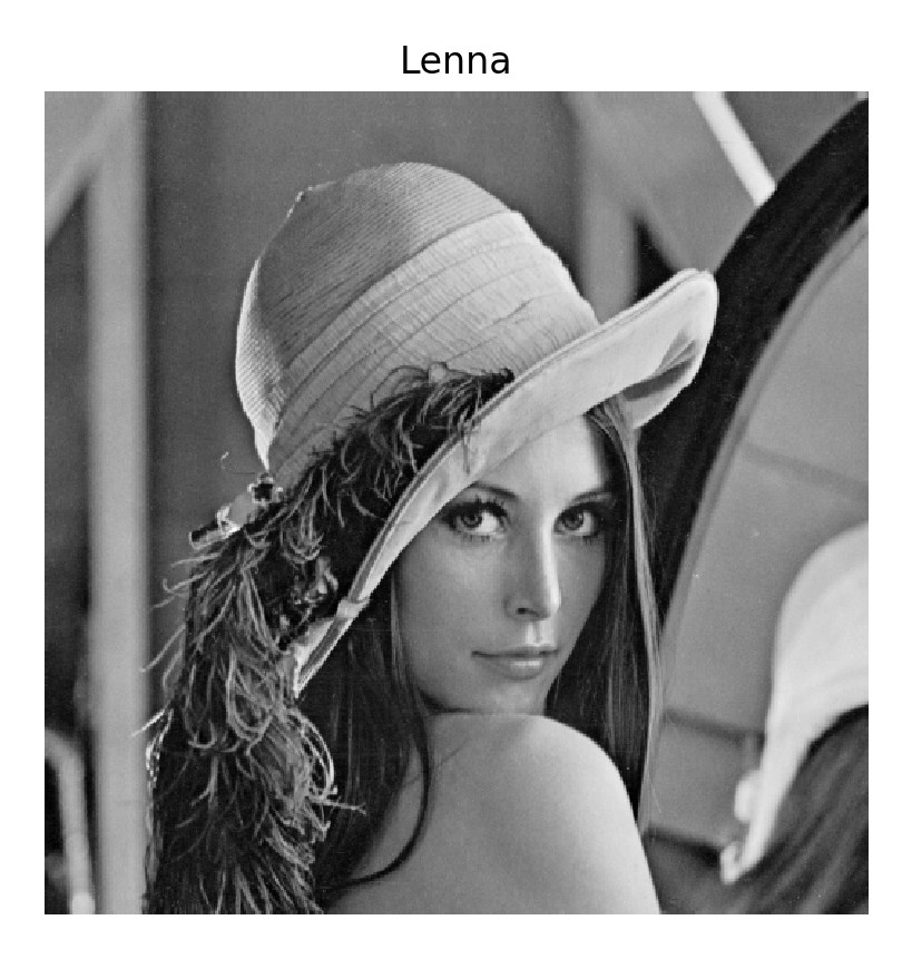
Figure 8: Lenna’s image

Here we consider three noise levels $\sigma\in\{0.1,0.2,0.3\}$. Note that the original image scale is $[0,1]$. Hence the image with noise level $\sigma=0.3$ is considered to be heavily blurred. The blurred images are shown in Figure 9.

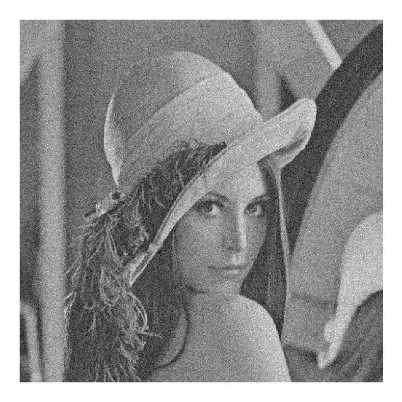
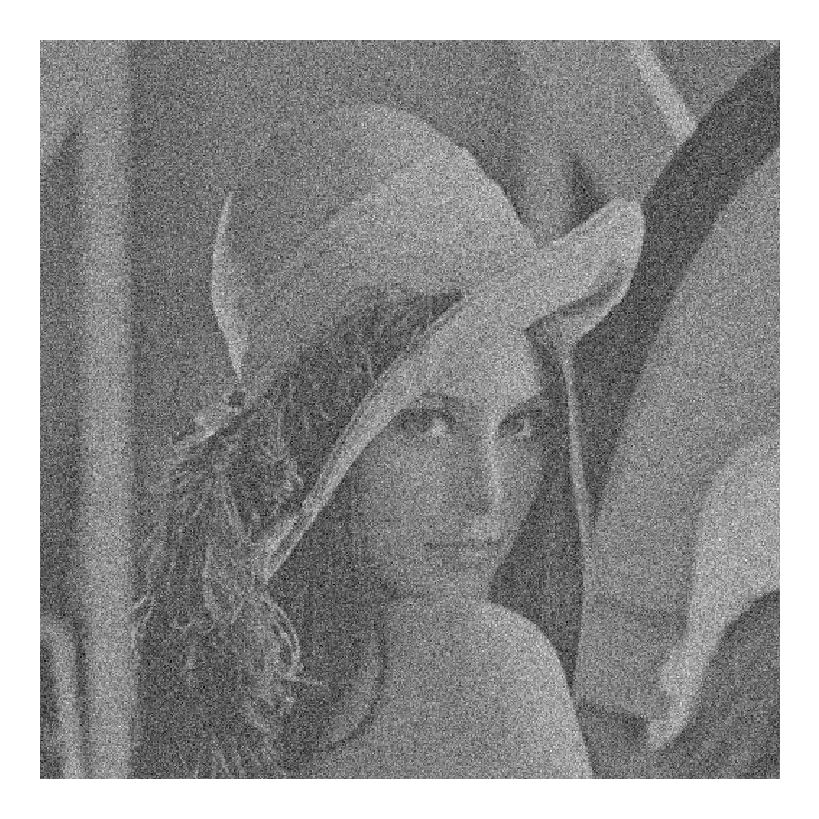
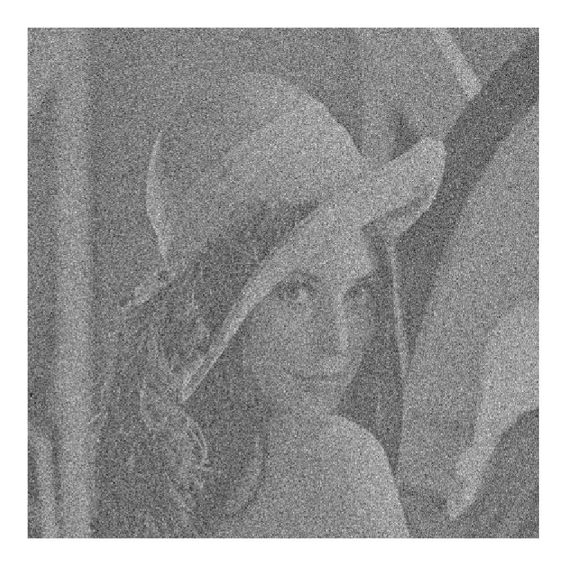
Figure 9: Lenna’s image with three noise levels $\sigma\in\{0.1,0.2,0.3\}$

For this real image, the configurations in the $h$KoPA model (1) is unknown. Therefore, we adopt the iterative greedy algorithm proposed in Section 3.2, where the configuration in each iteration is determined by BIC. For each $\bm{Y}_{\sigma}$, we consider to fit the image with at most 20 Kronecker product terms. The configurations selected $(\hat{m}_{k},\hat{n}_{k})$, the fitted $\hat{\lambda}_{k}$ and the cumulated percentage of variance explained (c.p.v.) for the first 10 iterations are reported in Table 1. It is seen that for all noise level $\sigma$ values, the first several Kronecker products terms can explain most of the variances of $\bm{Y}_{\sigma}$. With larger $\sigma$, $\lambda_{k}$ decreases slower as $k$ increases, because the residual matrix $\bm{E}^{(k)}$ has smaller variance. We also note that as the number of terms $k$ increases, configurations with smaller number of parameters tend to be selected, with some exceptions. This is partially because the residual matrix $\bm{E}^{(k)}$ tends to become less complex as higher level complexity tends to be explained by the earlier terms. Note that configuration $(6,7)$ has total $2^{6+7}+2^{3+2}-1=8223$ parameters, while $(4,5)$ has total $2^{4+5}+2^{5+4}-1=1023$ parameters. The proportion of variance of the true image $\bm{Y}$ is shown in the bottom row in Table 1. An overfitting is observed for $\sigma=0.3$ after the seventh iteration.

In the heavily blurred cases, configurations close to the center such as $(5,4)$ are more likely to be selected by BIC. These configurations correspond to more squared $\bm{A}_{k}$ and $\bm{B}_{k}$ matrices.

k	$\sigma=0.0$			$\sigma=0.1$			$\sigma=0.2$			$\sigma=0.3$
	$(\hat{m}_{k},\hat{n}_{k})$	$\hat{\lambda}_{k}$	c.p.v.	$(\hat{m}_{k},\hat{n}_{k})$	$\hat{\lambda}_{k}$	c.p.v.	$(\hat{m}_{k},\hat{n}_{k})$	$\hat{\lambda}_{k}$	c.p.v.	$(\hat{m}_{k},\hat{n}_{k})$	$\hat{\lambda}_{k}$	c.p.v.
1	(6, 7)	95.07	91.81	(5, 6)	91.21	66.76	(5, 6)	91.80	41.40	(4, 6)	88.28	23.21
2	(6, 6)	14.21	93.86	(5, 6)	21.88	70.60	(3, 6)	15.42	42.57	(4, 5)	26.97	25.37
3	(5, 7)	12.18	95.39	(5, 6)	19.48	73.65	(5, 4)	14.07	43.58	(4, 5)	18.05	26.34
4	(6, 6)	10.17	96.47	(4, 5)	8.00	74.16	(5, 4)	13.52	44.47	(3, 6)	17.37	27.24
5	(5, 6)	6.47	96.90	(5, 4)	7.66	74.63	(5, 4)	12.60	45.25	(4, 5)	15.68	27.97
6	(5, 5)	4.65	97.12	(4, 5)	7.00	75.03	(3, 6)	11.91	45.96	(4, 5)	15.24	28.66
7	(4, 5)	3.48	97.24	(4, 5)	6.67	75.39	(3, 6)	11.07	46.60	(3, 6)	14.70	29.32
8	(4, 5)	3.29	97.35	(5, 4)	6.40	75.72	(5, 4)	10.56	47.13	(4, 5)	13.84	29.90
9	(5, 5)	3.66	97.49	(5, 4)	6.19	76.03	(5, 4)	9.92	47.62	(4, 5)	13.76	30.47
10	(4, 5)	2.92	97.58	(5, 4)	6.05	76.32	(3, 6)	9.59	48.08	(2, 7)	13.63	31.00
$\bm{Y}$	-	-	100	-	-	79.01	-	-	48.38	-	-	29.32

Table 1: Configurations selected, the fitted $\hat{\lambda}_{k}$ and the cumulated percentage of variance explained (c.p.v.) for the first 10 iterations. Proportion of variance of the true image is shown in the bottom row

$k$	$\sigma=0.0$	$\sigma=0.1$	$\sigma=0.2$	$\sigma=0.3$
1
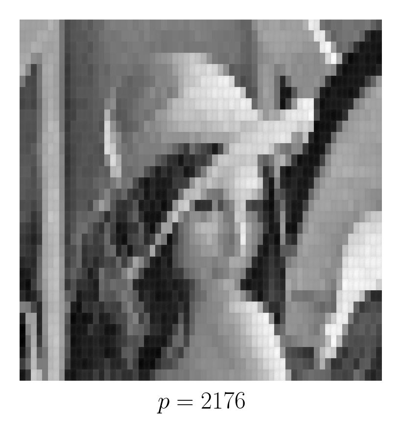
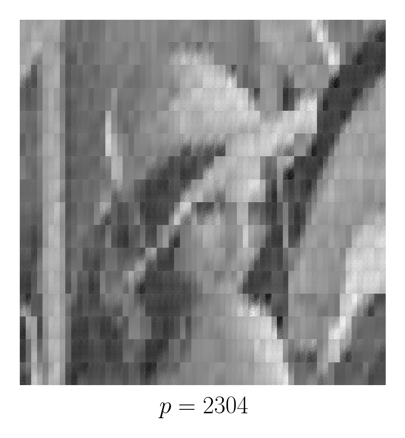
2
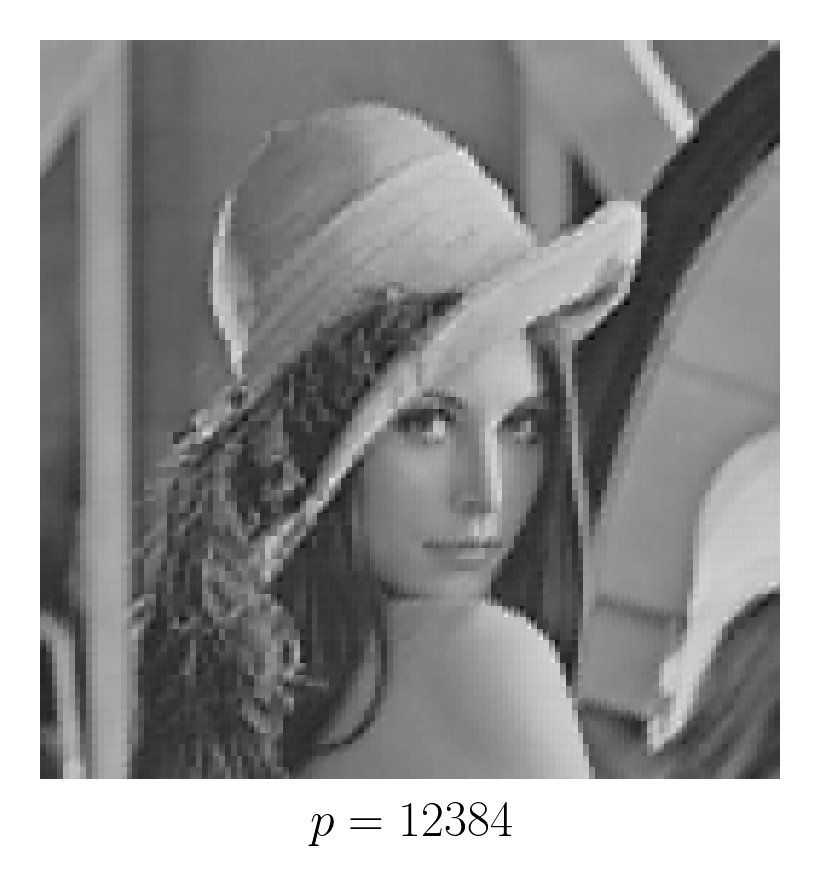
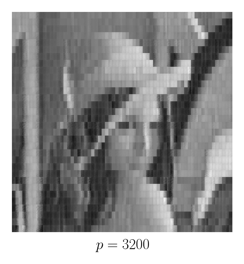
3
4
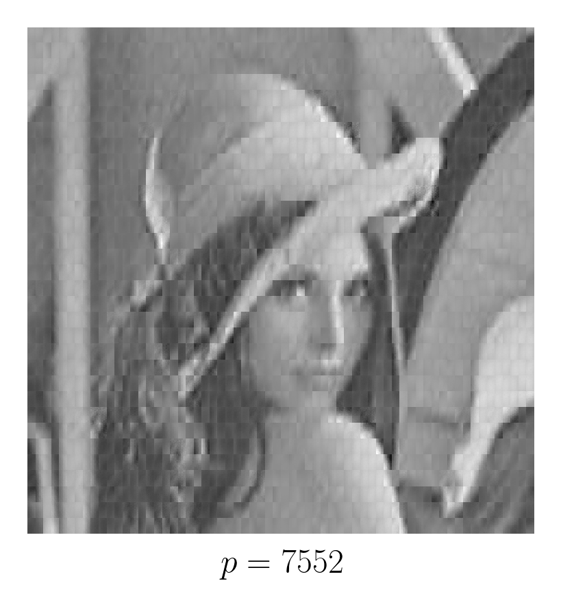
5
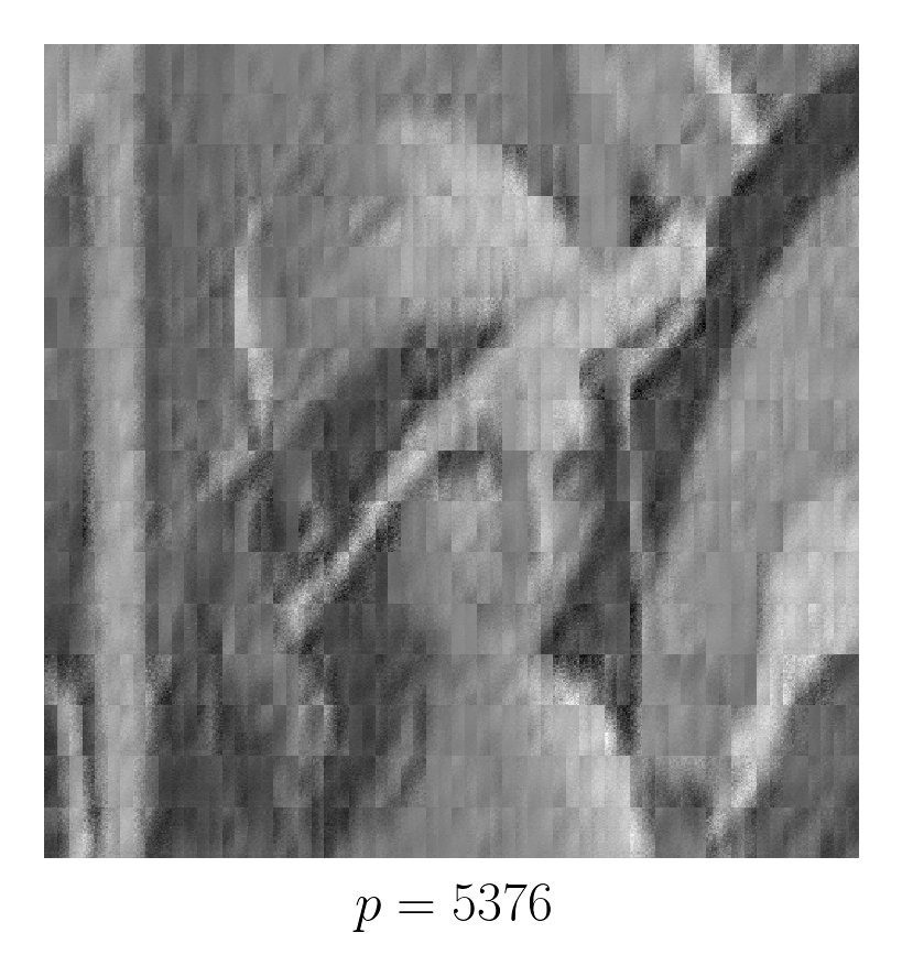
6

Figure 10: Fitted Images in the first 6 iterations.

The fitted images of using one to six Kronecker product terms at different noise levels $\sigma$ are plotted in Figure 10 with the number of parameters shown under each image. It is seen from the figures that, as expected, the smaller noise levels result in better recovery of the image with less numbers of Kronecker product terms. Note that the images plotted in Figure 10 are ordered according to the number of Kronecker product terms used instead of the number of parameters used. The configuration $(6,7)$ selected in the first iteration in the $\sigma=0$ case uses roughly four times the number of parameters of the configuration $(5,6)$ selected in the $\sigma=0.1$ case.

In additional to the iterative greedy algorithm, we use a stopping criterion based on random matrix theory to determine number of Kronecker products. Specifically, at iteration $k$, an estimate of $\sigma$ is

$$\hat{\sigma}=2^{-(M+N)/2}\|\hat{\bm{E}}^{(k)}-\hat{\bm{S}}_{k}\|_{F}=2^{-(M+N)/2}\|\hat{\bm{E}}^{(k+1)}\|_{F}.$$

Under the i.i.d. Gaussian assumption on $\hat{\bm{E}}^{(k+1)}$, we have

$$P\left[\|\mathcal{R}_{\hat{m}_{k},\hat{n}_{k}}[\hat{\bm{E}}_{k+1}]\|_{S}\geqslant\hat{\sigma}\left(2^{(\hat{m}_{k}+\hat{n}_{k})/2}+2^{(M+N-\hat{m}_{k}-\hat{n}_{k})/2}+t\right)\right]\leqslant e^{-t^{2}/2},$$

according to the non-asymptotic analysis on the random matrices (Vershynin, 2010). Here we set $t=\sqrt{2\log 100}\approx 3.03$ such that the probability is bounded by 0.01. We terminate the algorithm at step $k$ if

$$\hat{\lambda}_{k}\leqslant\hat{\sigma}\left(2^{(\hat{m}_{k}+\hat{n}_{k})/2}+2^{(M+N-\hat{m}_{k}-\hat{n}_{k})/2}+\sqrt{2\log 100}\right),$$ (7)

and use the first $\hat{K}=k-1$ terms as the optimal approximation. Specifically, when $\sigma=0$ or $0.1$, the stopping criterion is never met in the first $20$ iterations and we use $\hat{K}=20$. When $\sigma=0.2$, a 9-term model is selected, and when $\sigma=0.3$, the stopping criterion results in a 7-term model.

Singular value decomposition (SVD) is another widely used approach in image denoising and compression. It assumes

$$\bm{Y}=\sum_{i=1}^{K}\lambda_{i}\bm{u}_{i}\bm{v}_{i}^{T}.$$

The complexity level in such a approach is $K$, the number of rank one matrices used in the approximation. Note that SVD is a special case of $h$KoPA model in which each Kronecker product is a vector outer product, corresponding to configuration $(M,1)$ in KoPA model. Hence no configuration determination is needed. The number of parameters used in such an approximation is $K(2^{M}+2^{N}-1)$ where $K$ is the number of rank-one matrices used. To compare the performance of $h$KoPA with the SVD approach, we calculate the relative squared error of the fitted matrix $\hat{\bm{Y}}$ by

$$RSE=\dfrac{\|\bm{Y}-\hat{\bm{Y}}\|_{F}^{2}}{\|\bm{Y}\|_{F}^{2}},$$

where $\bm{Y}$ is the original image without noise and $\hat{\bm{Y}}$ is the fitted matrix of the noisy version $\bm{Y}_{\sigma}$. For different noise levels $\sigma$, we plot RSE against the number of parameters used in the approximation, shown in Figure 11 for both SVD approximation and $h$KoPA. Models with different number of terms are marked in Figure 11 and the $h$KoPA with the proposed random matrix stopping criterion is highlighted with a “$\bm{\star}$” marker. Comparing the error curve of SVD with the one of $h$KoPA, Figure 11 reveals that for any level of model complexity (or the number of parameters), $h$KoPA is more accurate than the standard low rank SVD approximation. When noises are added, overfitting is observed for both $h$KoPA and SVD approximation as the error (comparing to the true image) increases when too many terms are used, seen from the $U$-shape of the curves. The stopping criterion in (7) prevents the model from significantly overfitting. The realized relative error of the $h$KoPA with number of terms selected by (7) is close to the minimum attainable error, though the estimated number of terms is not the optimal one.

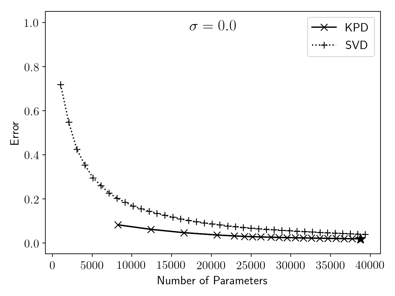
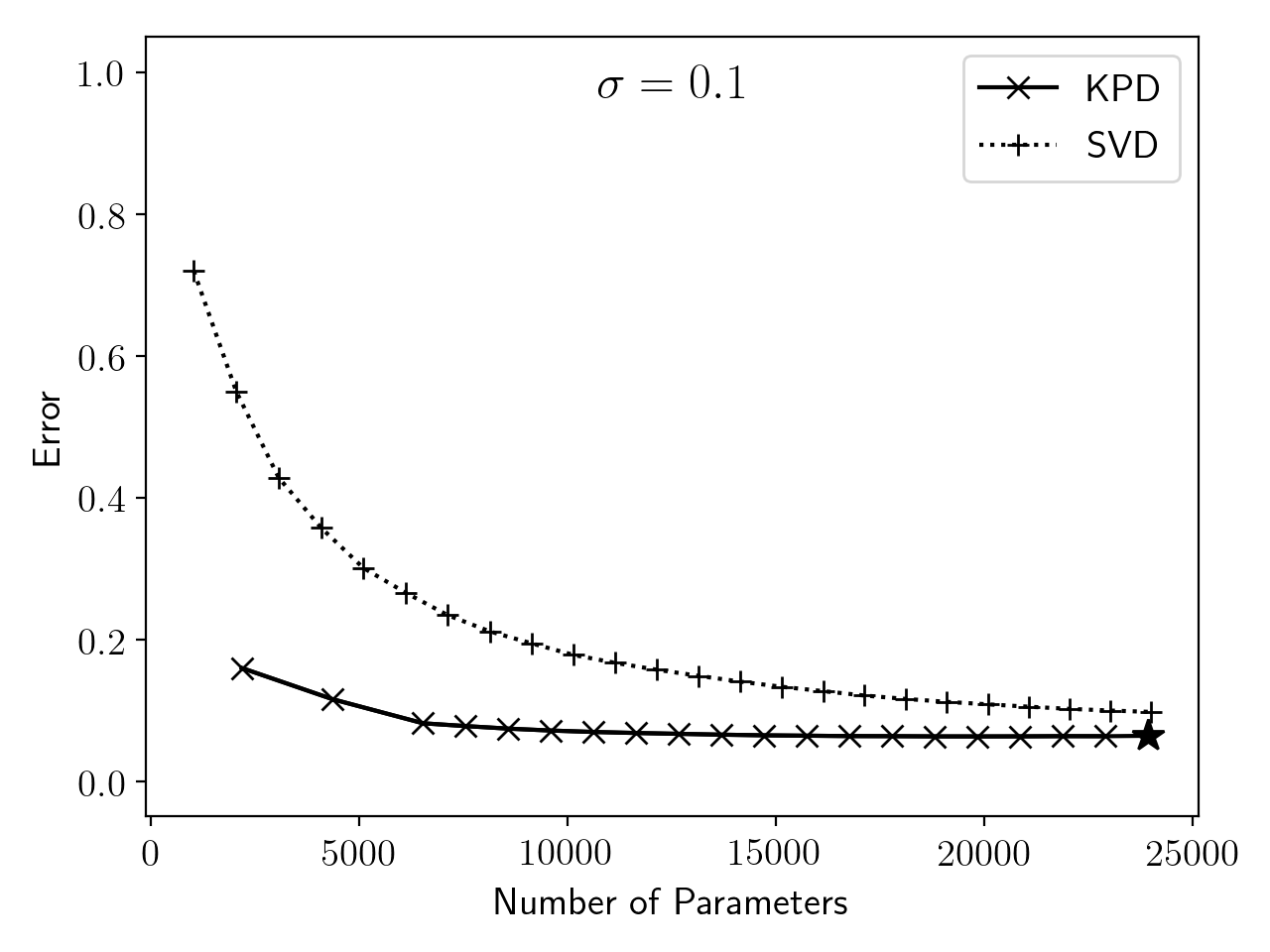
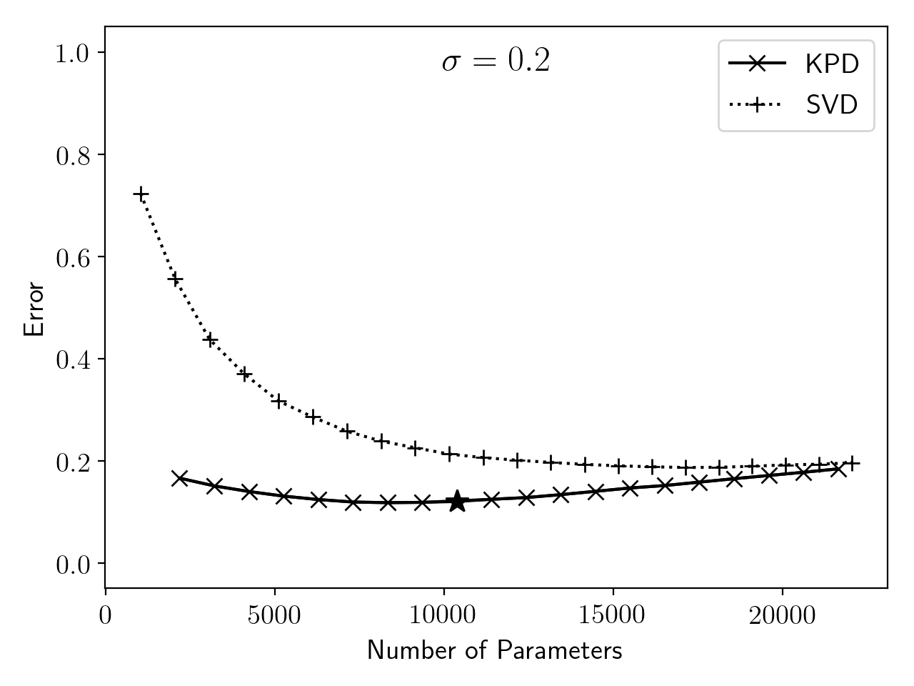
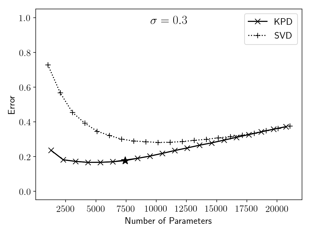
Figure 11: Error of fitted matrix against the number of parameters used.

5 Conclusion and Discussion

In this paper, we extend the single-term KoPA model proposed in Cai et al. (2019) to a more flexible setting, which allows multiple terms with different configurations and allows the configurations to be unknown. Identifiability conditions are studied to ensure unique representation of the model. And we propose two iterative estimation algorithms.

With a given set of configurations, we propose a least squares backfitting algorithm that fits each Kronecker product component in an alternating way. The simulation study shows the performance of the algorithm and the impact of the linear dependency between the component matrices.

When the configurations are unknown, the extra flexibility of $h$KoPA allows for more parsimonious representation of the underlying matrix, though it comes with the challenge of configuration determination. An iterative greedy algorithm is proposed to jointly determine the configurations and estimate each Kronecker product component. The algorithm iteratively adds one Kronecker product term to the model by finding the best one term KoPA to the residual matrix obtained from the previous iteration, using the procedure proposed in Cai et al. (2019). By analyzing a real image, we demonstrated that the proposed algorithm is able to obtain reasonable $h$KoPA and the results are significantly superior than the standard low rank matrix approximation using SVD.

The matrix dimensions discussed in this article are powers of 2. This is certainly not necessary. If the observed matrix is dimension $P\times Q$, and if $P$ has factors $1=p_{0}<p_{1}<\ldots<p_{M}=P$ and $Q$ has factors $1=q_{0}<q_{1}<\ldots<q_{N}=Q$, then the possible configuration set is all combinations of $(p_{m},q_{n})$ for $0\leq m\leq M$ and $0\leq n\leq N$, excluding the trivial $(1,1)$ and $(P,Q)$ cases. Note that $(P,1)$ configuration corresponds to the traditional low rank matrix SVD approximation setting. All algorithms presented in this paper apply for the general $P\times Q$ cases. Of course the more factors $P$ and $Q$ have, the larger the possible configuration set is hence we have more flexibility to find a better approximation. One can augment the observed matrix with additional rows and columns to increase the size of allowable configuration set. In image processing, a common tool used for augmentation is super-sampling by interpolating more pixels. In matrix denoising and compression, one can add zeros or duplicate certain rows and columns of the original matrix.

As discussed in Section 3, the greedy algorithm for configuration determination is similar to boosting algorithm. It can be improved at the expense of higher computational cost. In addition to combine it with the backfitting estimation procedure under a fixed configuration obtained by the greedy algorithm, the configurations can also be improved and adjusted under the backfitting framework. Their theoretical properties need to be investigated. A more sophisticated stopping criterion also needs to be investigated. Rrevious researches on principle component analysis rank determination such as those Minka (2001); Lam and Yao (2012); Bai et al. (2018) may be extended to our case.

References

- Akaike (1998) Akaike, H. (1998). Information Theory and an Extension of the Maximum Likelihood Principle, pages 199–213. Springer New York, New York, NY.
- Bai et al. (2018) Bai, Z., Choi, K. P., and Fujikoshi, Y. (2018). Consistency of AIC and BIC in estimating the number of significant components in high-dimensional principal component analysis. The Annals of Statistics, 46:1050–1076.
- Cai et al. (2019) Cai, C., Chen, R., and Xiao, H. (2019). KoPA: Automated Kronecker product approximation. preprint https://arxiv.org/abs/1912.02392.
- Cai et al. (2009) Cai, D., He, X., Wang, X., Bao, H., and Han, J. (2009). Locality preserving nonnegative matrix factorization. In Twenty-First International Joint Conference on Artificial Intelligence.
- Candes and Plan (2010) Candes, E. J. and Plan, Y. (2010). Matrix completion with noise. Proceedings of the IEEE, 98(6):925–936.
- Candès and Recht (2009) Candès, E. J. and Recht, B. (2009). Exact matrix completion via convex optimization. Foundations of Computational mathematics, 9(6):717.
- Duarte and Baraniuk (2012) Duarte, M. F. and Baraniuk, R. G. (2012). Kronecker compressive sensing. IEEE Transactions on Image Processing, 21(2):494–504.
- Eckart and Young (1936) Eckart, C. and Young, G. (1936). The approximation of one matrix by another of lower rank. Psychometrika, 1(3):211–218.
- Freund et al. (1999) Freund, Y., Schapire, R., and Abe, N. (1999). A short introduction to boosting. Journal-Japanese Society For Artificial Intelligence, 14(771-780):1612.
- Grasedyck et al. (2013) Grasedyck, L., Kressner, D., and Tobler, C. (2013). A literature survey of low-rank tensor approximation techniques. GAMM-Mitteilungen, 36(1):53–78.
- Guillamet and Vitrià (2002) Guillamet, D. and Vitrià, J. (2002). Non-negative matrix factorization for face recognition. In Catalonian Conference on Artificial Intelligence, pages 336–344. Springer.
- Hoyer (2004) Hoyer, P. O. (2004). Non-negative matrix factorization with sparseness constraints. Journal of machine learning research, 5(Nov):1457–1469.
- Kaye et al. (2007) Kaye, P., Laflamme, R., and Mosca, M. (2007). An introduction to quantum computing. Oxford University Press.
- Lam and Yao (2012) Lam, C. and Yao, Q. (2012). Factor modeling for high-dimensional time series: inference for the number of factors. The Annals of Statistics, 40(2):694–726.
- Le et al. (2016) Le, C. M., Levina, E., and Vershynin, R. (2016). Optimization via low-rank approximation for community detection in networks. The Annals of Statistics, 44(1):373–400.
- Minka (2001) Minka, T. P. (2001). Automatic choice of dimensionality for PCA. In Advances in neural information processing systems, pages 598–604.
- Pauca et al. (2004) Pauca, V. P., Shahnaz, F., Berry, M. W., and Plemmons, R. J. (2004). Text mining using non-negative matrix factorizations. In Proceedings of the 2004 SIAM International Conference on Data Mining, pages 452–456. SIAM.
- Sainath et al. (2013) Sainath, T. N., Kingsbury, B., Sindhwani, V., Arisoy, E., and Ramabhadran, B. (2013). Low-rank matrix factorization for deep neural network training with high-dimensional output targets. In 2013 IEEE international conference on acoustics, speech and signal processing, pages 6655–6659. IEEE.
- Schwarz (1978) Schwarz, G. (1978). Estimating the dimension of a model. Ann. Statist., 6(2):461–464.
- Van Loan and Pitsianis (1993) Van Loan, C. F. and Pitsianis, N. (1993). Approximation with Kronecker products. In Linear algebra for large scale and real-time applications, pages 293–314. Springer.
- Vershynin (2010) Vershynin, R. (2010). Introduction to the non-asymptotic analysis of random matrices. In Compressed Sensing.
- Werner et al. (2008) Werner, K., Jansson, M., and Stoica, P. (2008). On estimation of covariance matrices with Kronecker product structure. IEEE Transactions on Signal Processing, 56(2):478–491.
- Wold et al. (1987) Wold, S., Esbensen, K., and Geladi, P. (1987). Principal component analysis. Chemometrics and intelligent laboratory systems, 2(1-3):37–52.
- Yang and Leskovec (2013) Yang, J. and Leskovec, J. (2013). Overlapping community detection at scale: a nonnegative matrix factorization approach. In Proceedings of the sixth ACM international conference on Web search and data mining, pages 587–596. ACM.
- Yu et al. (2016) Yu, H.-F., Rao, N., and Dhillon, I. S. (2016). Temporal regularized matrix factorization for high-dimensional time series prediction. In Advances in neural information processing systems, pages 847–855.
- Yuan and Zhang (2016) Yuan, M. and Zhang, C.-H. (2016). On tensor completion via nuclear norm minimization. Foundations of Computational Mathematics, 16(4):1031–1068.
- Zhang et al. (2008) Zhang, T., Fang, B., Tang, Y. Y., He, G., and Wen, J. (2008). Topology preserving non-negative matrix factorization for face recognition. IEEE Transactions on Image Processing, 17(4):574–584.
- Zhang and Yeung (2012) Zhang, Y. and Yeung, D.-Y. (2012). Overlapping community detection via bounded nonnegative matrix tri-factorization. In Proceedings of the 18th ACM SIGKDD international conference on Knowledge discovery and data mining, pages 606–614. ACM.
- Zou et al. (2006) Zou, H., Hastie, T., and Tibshirani, R. (2006). Sparse principal component analysis. Journal of computational and graphical statistics, 15(2):265–286.