Linear encoding of the spatiotemporal cat

Abstract

The dynamics of an extended, spatiotemporally chaotic system might appear extremely complex. Nevertheless, the local dynamics, observed through a finite spatiotemporal window, can often be thought of as a visitation sequence of a finite repertoire of finite patterns. To make statistical predictions about the system, one needs to know how often a given pattern occurs. Here we address this fundamental question within a spatiotemporal cat, a 1-dimensional spatial lattice of coupled cat maps evolving in time. In spatiotemporal cat, any spatiotemporal state is labeled by a unique 2-dimensional lattice of symbols from a finite alphabet, with the lattice states and their symbolic representation related linearly (hence “linear encoding”). We show that the state of the system over a finite spatiotemporal domain can be described with exponentially increasing precision by a finite pattern of symbols, and we provide a systematic, lattice Green’s function methodology to calculate the frequency (i.e., the measure) of such states.

• November 15, 2020

Keywords: chaotic field theory, many-particle systems, coupled map lattices, periodic orbits, symbolic dynamics, cat maps

1 Introduction

While the technical novelty of this paper is in working out details of the spatiotemporal cat, an elegant, but very special model of many-particle dynamics (or discretization of a classical $d$-dimensional field theory), the vision that motivates it is much broader. We address here the long standing problem of how to describe, by means of discrete symbolic dynamics, the spatiotemporal chaos (or turbulence) in spatially extended, strongly nonlinear field theories.

One way to capture the essential features of turbulent motions of a physical flow is offered by coupled map lattice models, in which the spacetime is coarsely discretized, with the dynamics of domains that capture important small-scale spatial structures modeled by discrete time maps (Poincaré sections of a single “particle” dynamics) attached to lattice sites, and the coupling to neighboring sites consistent with the translational and reflection symmetries of the problem. Here we shall follow this path by investigating the Gutkin and Osipov [29] coupled cat maps lattice (“spatiotemporal cat” for short, in what follows), built from the Thom-Anosov-Arnol’d-Sinai cat maps (modeling the Hamiltonian dynamics of individual “particles”) at sites of a $1$-dimensional spatial lattice, linearly coupled to their nearest neighbors.

The key insight (which applies to coupled-map lattices in general, and PDEs modeled by them, not only the system considered here) is that a $2$-dimensional spatiotemporal pattern is best described by the corresponding $2$-dimensional spatiotemporal symbol lattice rather than by a one-dimensional temporal symbol sequence, as one usually does when describing a finite coupled “$N$-particle” system. The remarkable feature of the spatiotemporal cat is that its every solution is uniquely encoded by a linear transformation to the corresponding finite alphabet $2$-dimensional symbol lattice, a spatiotemporal generalization of the linear code for temporal evolution of a cat map, introduced in the beautiful 1987 paper by Percival and Vivaldi [40].

Within the spatiotemporal cat, a window into system dynamics is provided by a finite block of symbols, and the central question is to understand which symbol blocks are admissible, and what is the likelihood of a given block’s occurrence. It was already noted in [29] that two spatiotemporal orbits that share the same sub-block shadow each other exponentially well within the corresponding spatiotemporal window. This is the key property of hyperbolic spatiotemporal dynamics that we explore in detail in this paper. The linearity of the spatiotemporal cat enables us to go far analytically; lattice Green’s function methods enable us to compute explicitly the measures of a large set of spatiotemporally finite blocks, and give an algorithm for exact computation of the rest (which is computationally feasible for small blocks).

We start by formulating our “spatiotemporal cat” and stating the main results of the paper.

2 Model and overview of the main results

Spatiotemporal cat

Consider a linear, phase space (area) preserving map of a 2-torus $\mathbb{T}^{2}=\mathbb{R}^{2}/\mathbb{Z}^{2}$ onto itself

$$\left(\begin{array}[]{c}x_{t+1}\\ p_{t+1}\end{array}\right)=A\left(\begin{array}[]{c}x_{t}\\ p_{t}\end{array}\right)\quad\mbox{\rm mod}\,1\,,\qquad A=\left(\begin{array}[]{cc}s-1&1\\ s-2&1\\ \end{array}\right)\,,$$ (1)

where both $x_{t}$ and $p_{t}$ belong to the unit interval. For integer $s=\tr{A}>2$ the map is referred to as a cat map [5]. It is a fully chaotic Hamiltonian dynamical system, which, rewritten as a 2-step difference equation in $(x_{t-1},x_{t})$ takes a particularly simple form [40]

$$x_{t+1}-s\,x_{t}+x_{t-1}=-{m_{t}}\,,$$ (2)

with the unique integer “winding number” ${m_{t}}$ at every time step $t$ ensuring that $x_{t+1}$ lands in the given covering partition of the unit torus. While the dynamics is linear, the nonlinearity comes through the $(\mbox{\rm mod}\,1)$ operation, encoded in ${m_{t}}\in\mathcal{A}$, where $\mathcal{A}$ is finite alphabet of possible values for ${m_{t}}$.

The cat map is generalized to the spatiotemporal cat map by considering a 1-dimensional spatial lattice, with field $x_{n,t}$ at site $n$. If each site couples only to its nearest neighbors $x_{n\pm 1,t}$, and if we require (1) invariance under spatial translations, (2) invariance under spatial reflections, and (3) invariance under the space-time exchange, we arrive at the 2-dimensional Euclidean coupled cat map lattice:

$$x_{n,t+1}+x_{n,t-1}-{2s}\,x_{n,t}+x_{n+1,t}+x_{n-1,t}=-{m_{n,t}}\,.$$ (3)

The temporal cat map (2), and the spatiotemporal cat (3) can be brought into uniform notation by converting the spatiotemporal differences to discrete derivatives. This yields the discrete screened Poisson equation [21, 31] for the $2$-dimensional spatiotemporal cat

$$(-\Box+{2(s-2)})\,x_{z} = {m_{z}}\,,\qquad{x_{z}\in\mathbb{T}^{1}\,,\quad{m_{z}}\in\mathcal{A}\,,\quad z\in\mathbb{Z}^{2}}\,,$$ (4)

$$\mathcal{A}=\{-3,-2,\cdots,{2s}-2,{2s}-1\}\,,$$

where the Euclidean spacetime Laplacian is given by

$$\Box\,x_{t} \equiv x_{t+1}-2\,x_{t}+x_{t-1}$$ (5)

$$\Box\,x_{n,t} \equiv x_{n,t+1}+x_{n+1,t}-4\,x_{n,t}+x_{n,t-1}+x_{n-1,t}$$ (6)

in $d=1$ and $2$ dimensions, respectively, As in the $d=1$ case (2), the alphabet $\mathcal{A}$ ranges over all “winding number” ${m_{n,t}}$ values needed to ensure that the field $x_{n,t}$ on every lattice site is confined to the $\mbox{\rm mod}\,1$ interval $[0,1)$. The spatiotemporal cat is smooth and fully hyperbolic for integer ${s}>2$.

The key insight is that $2$-dimensional spatiotemporal lattice of integers $\{{m_{z}}\}=\{{m_{z}},z\in\mathbb{Z}^{{2}}\}$ is the natural encoding of a $2$-dimensional spatiotemporal state. As the relation (4) between the lattice state $\{x_{z}\}=\{x_{z},z\in\mathbb{Z}^{{2}}\}$ and its encoding $\{{m_{z}}\}$ is linear, we refer to ${m_{z}}$ as the “linear code” following [40], both for the cat map (2) in one dimension, and for the spatiotemporal cat (4) in two dimensions. Given a set of $\{{m_{z}}\}$, the linearity of (4) enables us to determine the corresponding lattice state $\{x_{z}\}$ by Green’s function methods.

This paper builds explicit 2-dimensional spatiotemporal cat symbolic dynamics using winding numbers ${m_{z}}$ and Green’s functions with Dirichlet boundary conditions. The companion paper [18] formulates the periodic orbit theory for $d$-dimensional spatiotemporal cat using Green’s functions with periodic boundary conditions.

Statement of the problem

As spatiotemporal cat (4) is a Hamiltonian system, it possesses the natural measure ${\mu}$ (see B) invariant under space and time translations. Let $\mathsf{X}=\{x_{z}\in\mathbb{T}^{1},\,z\in\mathbb{Z}^{2}\}$ be a spatiotemporally infinite solution of $d=2$ spatiotemporal cat, generated by initial conditions generic with respect to ${\mu}$ in the fully hyperbolic regime $s>2$. By the linear relation between $\mathsf{X}$ and $\mathsf{M}$, symbolic representation of $\mathsf{X}$ is given by a unique block $\mathsf{M}=\{{m_{z}}\in\mathcal{A}\,,\;z\in\mathbb{Z}^{2}\}\,.$ Assuming now that only partial information is available, over a finite lattice domain $\mathcal{R}\subset\mathbb{Z}^{2}$, we would like to know the probability that $\mathsf{M}$  has prescribed set of symbols $\mathsf{M}_{\mathcal{R}}$ over $\mathcal{R}$. Slightly rephrased, the central question studied in this paper are the relative frequencies $f(\mathsf{M}_{\mathcal{R}})$ of symbol blocks within the symbolic representation of a generic spatiotemporal pattern:

Q1. How often does a prescribed finite symbol block $\mathsf{M}_{\mathcal{R}}$ occur in the symbolic representation $\mathsf{M}$ of a generic state $\mathsf{X}$?

Our second question is about information stored in a finite symbol block $\mathsf{M}_{\mathcal{R}}$. For the standard cat map symbolic dynamics based on a finite Markov partition of the cat map phase space, a 1-dimensional block of symbols defines the corresponding trajectory up to an error which decreases exponentially with the length of the symbol block [10, 44, 12]. We would like to know whether the corresponding result holds for $2$-dimensional linear encoding:

Q2. To what precision does the symbol block $\mathsf{M}_{\mathcal{R}}$ define the local spatiotemporal pattern ${\mathsf{X}_{\mathcal{R}}}=\{x_{z}\in\mathbb{T}^{1},\,z\in\mathcal{R}\}$ ?

Main results

Let $\mathcal{R}=\{(n,t)\,|\,n=1,\dots,\ell_{1},t=1,\dots\ell_{2}\}$ be a rectangular domain of the lattice (an $[\ell_{1}\!\times\!\ell_{2}]$ spatiotemporal window), and let $\mathsf{M}_{\mathcal{R}}$ be a $[\ell_{1}\!\times\!\ell_{2}]$ block of symbols from the alphabet $\mathcal{A}$. Given a generic solution $\mathsf{X}$ of the equation (3) and its symbolic representation $\mathsf{M}=\{{m_{nt}}\,|\,(n,t)\in\mathbb{Z}^{2}\}$ the space (resp. time) shift action on it is given by

$$\mathcal{S}\cdot\mathsf{M}=\{{m_{n+1,t}}\,|\,(n,t)\in\mathbb{Z}^{2}\}\,,\qquad\mathcal{T}\cdot\mathsf{M}=\{{m_{n,t+1}}\,|\,(n,t)\in\mathbb{Z}^{2}\}\,.$$ (7)

How often $\mathsf{M}_{\mathcal{R}}$ occurs within $\mathsf{M}$ is then defined by the double limit

$$f(\mathsf{M}_{\mathcal{R}})=\lim_{T,L\to\infty}\frac{1}{LT}\sum_{t=1}^{T}\sum^{L}_{n=1}\chi(\mathcal{S}^{n}\,\mathcal{T}^{t}\cdot\mathsf{M}\,|\,\mathsf{M}_{\mathcal{R}}),$$ (8)

where $\chi(\mathcal{S}^{n}\,\mathcal{T}^{t}\cdot\mathsf{M}\,|\,\mathsf{M}_{\mathcal{R}})$ is the characteristic function that equals to $1$ if symbols of $\mathcal{S}^{n}\,\mathcal{T}^{t}\cdot\mathsf{M}$ coincide with $\mathsf{M}_{\mathcal{R}}$ over $\mathcal{R}$, and equals to $0$ otherwise.

The $d=2$ spatiotemporal cat  is fully hyperbolic for ${s>2}$, see (79). On the basis of our numerical simulations, we conjecture that the natural measure ${\mu}$, invariant under spatial and temporal shifts $\mathcal{S}$, $\mathcal{T}$, is uniquely ergodic, with the initial conditions for $\mathsf{X}$ chosen to be generic with respect to ${\mu}$. In this case the limiting frequencies $f(\mathsf{M}_{\mathcal{R}})$ for generic solutions $\mathsf{X}$ of (3) are equal to the measures ${\mu}({\cal M}_{\mathcal{R}})$ of the cylinder sets ${\cal M}_{\mathcal{R}}$, defined as sets of spatiotemporal states $\mathsf{X}$ with the same $\mathsf{M}_{\mathcal{R}}$ block over the domain $\mathcal{R}$. For this reason, we shall refer to the frequencies estimated by (8) as measures of $\mathsf{M}_{\mathcal{R}}$, and denote them by ${\mu}(\mathsf{M}_{\mathcal{R}})$ in what follows.

Answer to Q1. The spatiotemporal cat admits a natural 2-dimensional linear encoding with a finite alphabet. We find it helpful to split the alphabet into two parts,

$$\mathcal{A}=\mathcal{A}_{0}\cup\mathcal{A}_{1}\,,$$

where the number of symbols in the exterior alphabet $\mathcal{A}_{1}$ is fixed, and the interior alphabet $\mathcal{A}_{0}$ is a full shift, with the number of symbols in $\mathcal{A}_{0}$ growing linearly with $s$. The following holds:

• Any block of symbols from $\mathcal{A}_{0}$ is admissible.

For any general spatiotemporal ergodic system, relative frequencies $f(\mathsf{M}_{\mathcal{R}})$ defined by (8) provide a numerical way to estimate measures ${\mu}(\mathsf{M}_{\mathcal{R}})$, by generating solutions on finite $[{L}\!\times\!{T}]$ domains, compatible everywhere locally with the defining equation (4), and counting the number of times $\mathsf{M}_{\mathcal{R}}$ occurs within each such solution. However, due to the linear relation between a spatiotemporal state $\mathsf{X}$ and its symbolic encoding $\mathsf{M}$, for the spatiotemporal cat one can do much better, and compute measures ${\mu}(\mathsf{M}_{\mathcal{R}})$ analytically and explicitly:

• Measures of blocks $\mathsf{M}_{\mathcal{R}}$ are given by rational numbers and factorize into products of constant and geometrical parts:

  $${\mu}(\mathsf{M}_{\mathcal{R}})=d_{\mathcal{R}}|\mathcal{P}(\mathsf{M}_{\mathcal{R}})|\,.$$

  The constant $d_{\mathcal{R}}$ depends only on domain $\mathcal{R}$, independent of the symbolic content $M_{\mathcal{R}}$. The factor $|\mathcal{P}(\mathsf{M}_{\mathcal{R}})|$ admits geometrical interpretation as the volume of polytope $\mathcal{P}(\mathsf{M}_{\mathcal{R}})$ in the $|\partial\mathcal{R}|$-dimensional Euclidean space, where $|\partial\mathcal{R}|$ is the number of boundary points of the domain $\mathcal{R}$. The polytope $\mathcal{P}(\mathsf{M}_{\mathcal{R}})$ is determined by the content of $\mathsf{M}_{\mathcal{R}}$. For small $|\mathcal{R}|$, ${\mu}(\mathsf{M}_{\mathcal{R}})$ can be evaluated analytically, see sections 3.5 and 4.3.

• If $\mathsf{M}_{\mathcal{R}}$ is composed only of symbols from $\mathcal{A}_{0}$, then $|\mathcal{P}(\mathsf{M}_{\mathcal{R}})|=1$ and ${\mu}(\mathsf{M}_{\mathcal{R}})=d_{\mathcal{R}}$.

Answer to Q2. The block of symbols $\mathsf{M}_{\mathcal{R}}$ defines the spatiotemporal state $\mathsf{X}$ over $\mathcal{R}$ up to an error which decreases exponentially with the size of the domain $\mathcal{R}$:

• The difference between any solution $x_{z_{0}}$ of (4) for $z_{0}\in\mathcal{R}$ and the “average coordinate” $\bar{x}({\mathsf{M}_{\mathcal{R}}})$, determined solely by $\mathsf{M}_{\mathcal{R}}$, is bounded by

  $$|x_{z_{0}}-\bar{x}({\mathsf{M}_{\mathcal{R}}})|\leq Ce^{-\nu\ell(z_{0},\partial\mathcal{R})}\,,\qquad\nu>0,$$ (9)

  where $\ell(z_{0},\partial\mathcal{R})$ is the minimal Euclidean distance between $z_{0}$ and the boundary $\partial\mathcal{R}$. For explicit formulas for $\bar{x}({\mathsf{M}_{\mathcal{R}}})$ in terms of the block of symbols ${\mathsf{M}_{\mathcal{R}}}$ see (24) and (40).

Two remarks are in order. First, all of the above results hold also for the $d=1$ temporal cat map if $s>2$, see section 3. In this case, the domain $\mathcal{R}$ is just an interval in $\mathbb{Z}$ with two endpoints, $|\partial\mathcal{R}|=2$. Second, it is plausible that our results hold for spatiotemporal cat (4) on a lattice of dimension $d$, provided that $s>2$, i.e., the system is in the chaotic regime, but, in order to streamline the exposition, we discuss here only the 1- and 2-dimensional cases.

In principle, having answers to Q1 and Q2 allows for a calculation of the expectation values of observables by means of symbolic dynamics. As $\mathsf{M}_{\mathcal{R}}$ defines positions of points in the center $z_{0}$ of domain $\mathcal{R}$ with exponential precision, any observable $A(z)$ can be viewed as a function of $\mathsf{M}_{\mathcal{R}}$, $A(z_{0})\approx A\left(\mathsf{M}_{\mathcal{R}}\right)$, where the quality of the approximation increases exponentially with the size of $\mathcal{R}$. In the limit of large domain size $|\mathcal{R}|$, one approximates the sum over states of the lattice with exponentially increasing accuracy, and has for the average of $A$

$$\langle A\rangle=\lim_{|\mathcal{R}|\to\infty}\sum_{\mathsf{M}_{\mathcal{R}}}{\mu}(\mathsf{M}_{\mathcal{R}})A\left(\mathsf{M}_{\mathcal{R}}\right)\,,$$ (10)

where the sum is over all admissible blocks of symbols within $\mathcal{R}$. In particular, for $A=-\frac{1}{|\mathcal{R}|}\log{\mu}(\mathsf{M}_{\mathcal{R}})$ the above expression defines the spatiotemporal metric entropy of the system.

The paper is organized as follows: Section 3 is devoted to the cat map linear encoding, introduced in section 3.1. Its basic properties and the properties of the corresponding phase space partitions are established in section 3.2 and section 3.3. In section 3.4 we investigate the measures of admissible finite symbol blocks, and show their factorization into a geometric part, and a constant part which depends only on the length of the block. We evaluate explicitly the geometrical part of measures for short blocks of symbols in section 3.5. The key conceptual ingredient that underpins this calculation, hidden in much algebra in what follows, are the transformations (31) and (42) from the Hamiltonian initial state formulation to the Lagrangian end points formulation. This replaces the exponentially unstable Hamiltonian time evolution problem by a robustly convergent Lagrangian boundary value problem.

In section 4, we extend these results to the spatiotemporal cat. We show in section 4.1 that the system admits a natural 2-dimensional linear encoding with a finite alphabet, and then compute the measures of finite spatiotemporal symbol blocks in section 4.2. In section 5, we use these results to construct sets of spatiotemporal invariant 2-tori that fully shadow each other. Implementing this program requires extensive use of lattice Green’s functions, whose properties are derived in A. The Hamiltonian formulation of the spatiotemporal cat map and the metric entropy estimation are provided in B and C, respectively. The results are summarized and some open questions discussed in the section 6.

3 Cat map

Before turning to the “many-particle” case, it is instructive to motivate our formulation of the spatiotemporal cat by investigating the cat map (i.e., a “spatial lattice” with only one site). We start by a brief review of the physical origin of cat maps.

Phase space area-preserving maps that describe kicked rotors subject to a discrete time sequence of angle-dependent impulses $F(x_{t})$, $t\in\mathbb{Z}$,

$$x_{t+1} = x_{t}+p_{t+1}\qquad\mbox{\rm mod}\,1,$$ (11)

$$p_{t+1} = p_{t}+F(x_{t})\,,$$ (12)

play important role in the theory of chaos in Hamiltonian systems, from the Taylor, Chirikov and Greene standard map [36, 14], to the cat maps that we study here. Here $2\pi x$ is the angle of the rotor, $p$ is the momentum conjugate to the configuration coordinate $x$, $F(x)=F(x+1)$ is periodic with period $1$, and the time step has been set to $\Delta t=1$. Eq. (11) says that in one time step $\Delta t$ the configuration trajectory starting at $x_{t}$ reaches $x_{t+1}=x_{t}+p_{t+1}\Delta t$, and (12) says that at each kick the angular momentum $p_{t}$ is accelerated to $p_{t+1}$ by the force pulse $F(x_{t})\Delta t$. As the values of $x$ differing by integers are identified, and the momentum $p$ is unbounded, the phase space is a cylinder. However, to analyse the dynamics, one can just as well compactify the phase space by folding the momentum dynamics onto a circle, by adding “$\mbox{\rm mod}\,1$” to (12). This reduces the dynamics to a toral automorphism acting on a $[0,1)\times[0,1)$ square of unit area, with the opposite sides identified.

The simplest example of (11,12) is a rotor subject to a force $F(x)=Kx$ linear in the displacement $x$. The $\mbox{\rm mod}\,1$ added to (12) makes this a discontinuous “sawtooth,” unless $K$ is an integer. In that case the map (11,12) is a continuous automorphism of the torus, or a “cat map” [5], a linear symplectic map on the unit 2-torus phase space, $(x\mapsto Ax\,|\,x\in\mathbb{T}^{2}=\mathbb{R}^{2}/\mathbb{Z}^{2}\,;\;A\in SL(2,\mathbb{Z}))\,,$ with coordinates $x=(x_{t},p_{t})$ interpreted as the angular position variable and its conjugate momentum at time instant $t$. Explicitly:

$$\left(\begin{array}[]{c}x_{t+1}\\ p_{t+1}\end{array}\right)=A\left(\begin{array}[]{c}x_{t}\\ p_{t}\end{array}\right)\quad\mbox{\rm mod}\,1\,,\qquad{A}=\left(\begin{array}[]{cc}a&c\\ d&b\end{array}\right)\,,$$ (13)

where $a,b,c,d$ are any integers that satisfy $\det A=1$, so that the map is symplectic (area preserving).

A cat map is a fully chaotic Hamiltonian dynamical system if its stability multipliers $(\Lambda\,,\;\Lambda^{-1})$, where

$$\Lambda=(s+\sqrt{(s-2)(s+2)})/2\,,\qquad\Lambda=e^{\lambda}\,,$$ (14)

are real, with a positive Lyapunov exponent $\lambda>0$. The eigenvalues are functions of a single parameter $s=\tr{A}=\Lambda+\Lambda^{-1}$, and the map is chaotic if and only if $|s|>2$. We shall refer here to the least unstable of the cat maps (13), with $s=3$, as the “Arnol’d”, or “Arnol’d-Sinai cat map” [5, 20], and to general maps with integer $s\geq 3$ as “cat maps”. Cat maps have been extensively analyzed as particularly simple examples of chaotic Hamiltonian dynamics. They exhibit ergodicity, mixing, exponential sensitivity to variation of the initial conditions (the positivity of the Lyapunov exponent), and the positivity of the Kolmogorov-Sinai entropy [48]. Detailed understanding of dynamics of cat maps is important also for the much richer world of nonlinear hyperbolic toral automorphisms, see [16, 24, 47] for examples.

3.1 Linear encoding

Eqs. (11,12) are the discrete-time Hamilton’s equations, which induce temporal evolution on the 2-torus $(x_{t},p_{t})$ phase space. For the problem at hand, it pays to go from the Hamiltonian $(x_{t},p_{t})$ phase space formulation to the Newtonian $(x_{t-1},x_{t})$ state space formulation [40], with $p_{t}$ replaced by $p_{t}=(x_{t}-x_{t-1})/\Delta t\,.$ Eq. (12) then takes the 2-step difference form (the discrete time Laplacian $\Box$ formula for the second order time derivative ${d^{2}}/{dt^{2}}$, with the time step set to $\Delta t=1$),

$$\Box\,x_{t}\equiv x_{t+1}-2x_{t}+x_{t-1}=F(x_{t})\qquad\mbox{\rm mod}\,1\,,$$ (15)

i.e., Newton’s Second Law: “acceleration equals force.” For a cat map, with force $F(x)$ linear in the displacement $x$, the Newton’s equation of motion (15) takes the form

$$(\Box+2-s)\,x_{t}=-{m_{t}}\,,$$ (16)

with $\mbox{\rm mod}\,1$ enforced by ${m_{t}}$’s, integers from the alphabet

$$\mathcal{A}=\{\underline{1},0,\dots s\!-\!1\}\,,$$ (17)

necessary to keep $x_{t}$ for all times $t$ within the unit interval $[0,1)$. For the sake of notational convenience, we have introduced here the symbol $\underline{m_{t}}$ to denote $m_{t}$ with the negative sign, i.e., ‘$\underline{1}$’ stands for the symbol ‘$-1$’.

Figure 1: (Color online) The Newtonian $s=3$ Arnol’d cat map matrix $A^{\prime}$ (18) keeps the origin $(0,0)$ fixed, but otherwise stretches the unit square into a parallelogram. Translations by ${m_{0}}$ from alphabet $\mathcal{A}=\{\underline{1},0,1,2\}=$ {red, green, blue, yellow} bring stray regions back onto the torus.

3.2 Percival-Vivaldi linear encoding partition of the state space

To interpret ${m_{t}}$’s, consider the action of the Newtonian cat map (16) on a 2-dimensional state space point $(x_{t-1},x_{t})$,

$$\left(\begin{array}[]{c}x_{t}\\ x_{t+1}\end{array}\right)=A^{\prime}\left(\begin{array}[]{c}x_{t-1}\\ x_{t}\end{array}\right)-\left(\begin{array}[]{c}0\\ {m_{t}}\end{array}\right)\,,\qquad{A^{\prime}}=\left(\begin{array}[]{cc}0&1\\ -1&s\end{array}\right)\,.$$ (18)

In Percival and Vivaldi [40], this representation of cat map is referred to as “the two-configuration representation”. As illustrated in figure 1, in one time step the area preserving map $A^{\prime}$ stretches the unit square into a parallelogram, and a point $(x_{0},x_{1})$ within the initial unit square in general lands outside it, in another unit square ${m_{t}}$ steps away. As they shepherd such stray points back into the unit torus, the integers ${m_{t}}$ can be interpreted as “winding numbers” [34], or “stabilising impulses” [40]. The ${m_{t}}$ translations reshuffle the state space, thus partitioning it into $|\mathcal{A}|$ regions ${\cal M}_{m}$, ${m}\in\mathcal{A}$.

As illustrated by figure 1, there are the two kinds of pieces within the state space partition: the parallelograms ${\cal M}_{0},\dots,{\cal M}_{s-2}$, and the two exterior half sized triangles ${\cal M}_{\underline{1}}$, ${\cal M}_{s-1}$, labeled by the $(s\!-\!1)$-letter interior alphabet $\mathcal{A}_{0}$, and the two-letter exterior alphabet $\mathcal{A}_{1}$, respectively. For integer $s\geq 2$ these alphabets are

$$\mathcal{A}=\mathcal{A}_{0}\cup\mathcal{A}_{1}\,,\qquad\mathcal{A}_{0}=\{0,\cdots,s\!-\!2\}\,,\qquad\mathcal{A}_{1}=\{\underline{1},s\!-\!1\}\,.$$ (19)

Refinements of these partitions work very much like they do for the baker’s map and the Smale horseshoe, by peering further into the future and the past, and constructing the intersections of the future and past partitions [17]. The “$\ell$-th level” of partition ${\cal M}=\cup{\cal M}_{b}$ is labeled by the set of all admissible blocks $b$ of length $\ell$, composed of the past $\ell-t-1$ steps, and future $t$ steps, with ‘decimal point’ denoting the present,

$$b={m_{t-\ell+1}}\cdots{m_{-1}}{m_{0}}.{m_{1}}{m_{2}}\cdots{m_{t}}\,.$$

For the cat map symbol blocks $\mathsf{M}_{\mathcal{R}}$ is 1-dimensional, and a domain $\mathcal{R}$ consists of $\ell$ consecutive temporal lattice sites, so in this section we shall denote $\mathsf{M}_{\mathcal{R}}$ by a block $b$ of length $\ell$, and refer to the infinite length symbol block as ‘itinerary’.

While an admissible infinite itinerary defines a unique point in the state space, a finite block $b$ determines a cylinder set ${\cal M}_{b}$, the set of all points in $(x_{0},x_{1})$ plane having itineraries of the form

$$\cdots a_{t-\ell-1}a_{t-\ell}{m_{t-\ell+1}}\cdots{m_{-1}}{m_{0}}.{m_{1}}{m_{2}}\cdots{m_{t}}a_{t+1}a_{t+2}\cdots\,,$$

with fixed ${m_{i}}$’s, and arbitrary $a_{i}\in\mathcal{A}$. How these blocks partition the state space is best understood by inspecting figure 2.

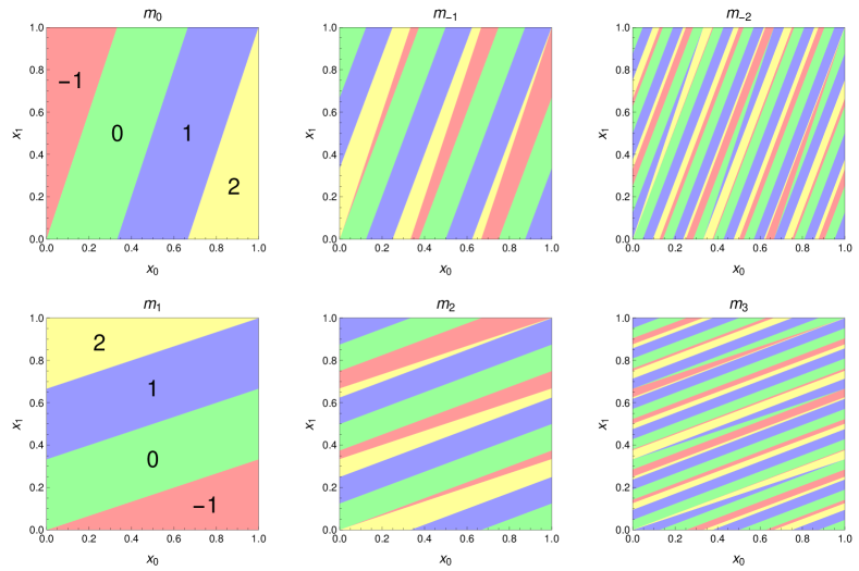
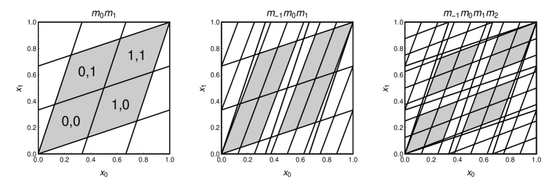
Figure 2: (Color online) Arnol’d cat map $(x_{0},x_{1})$ state space partition into (a) 4 regions labeled by ${m_{0}}.$ , obtained from $(x_{-1},x_{0})$ state space by one iteration (the same as figure 1). (b) 14 regions labeled by past block ${m_{-1}}{m_{0}}.$, obtained from $(x_{-2},x_{-1})$ state space by two iterations. (c) 44 regions, past block ${m_{-2}}{m_{-1}}{m_{0}}.$ (d) 4 regions labeled by $.{m_{1}}$ , obtained from $(x_{2},x_{1})$ state space by one backward iteration. (e) 14 regions labeled by future block $.{m_{1}}{m_{2}}$ , obtained from $(x_{3},x_{2})$ state space by two backward iterations. (f) 44 regions, future block ${m_{3}}{m_{2}}{m_{1}}.$ Each color has the same total area ($1/6$ for ${m_{t}}=\underline{1},2$, and $1/3$ for ${m_{t}}=0,1$). State space partition into (g) 14 regions labeled by block $b={m_{0}}.{m_{1}}$, the intersection of one past (a) and one future iteration (d). (h) block $b={m_{-1}}{m_{0}}.{m_{1}}$, the intersection of two past (b) and one future iteration (d). (i) block $b={m_{-1}}{m_{0}}.{m_{1}}{m_{2}}$, the intersection of two past (b) and two future iterations (e). Note that while some regions involving external alphabet (such as $\_{22}\_$ in (g)) are pruned, the interior alphabet labels a horseshoe, indicated by the shaded regions. The first three covers of the horseshoe have areas (g) $4\times 1/8$, (h) $8\times 1/21$, and (i) $16\times 1/55$. All boundaries are straight lines with rational slopes.

	1	0	1	2
1	0	0.0208	0.0625	0.0833
0	0.0208	0.1250	0.1250	0.0625
1	0.0625	0.1250	0.1250	0.0208
2	0.0833	0.0625	0.0208	0

	1	0	1	2
1	0	1/48	1/16	1/12
0	1/48	1/8	1/8	1/16
1	1/16	1/8	1/8	1/48
2	1 /12	1/16	1/48	0

Table 1: The measures ${\mu}({m_{i}}{m_{i+1}})$ of the 16 distinct 2-symbol blocks ${m_{i}}{m_{i+1}}$ for the $s=3$ Arnol’d cat map, (left) obtained from a long-time ($\sim 10^{9}$ iterations) numerical simulation rounded off to four significant digits; (right) the exact values given by (34), or read off as sub-partition areas in figure 2 (g). Column:  ${m_{i}}$. Row:  ${m_{i+1}}$. See figure 2 for a geometric picture of why blocks $\underline{1}\underline{1}$ and $22$ are pruned.

3.3 From itineraries to orbits and back

The power of the linear encoding for a cat map [40] is that one can use integers ${m_{t}}$ to encode its state space trajectories. Since the connection (16) between sequences of ${m_{t}}$ and $x_{t}$ is linear, it is straightforward to go back and forth between state space and symbolic representation of an orbit. In particular, if $\{{m_{t}}\}$ is an admissible itinerary, the corresponding state space point at the $t$ time instant is given by the inverse of (16),

$$x_{t}=\sum_{t^{\prime}=-\infty}^{\infty}\mathsf{g}_{tt^{\prime}}{m_{t^{\prime}}}\,,\qquad\mathsf{g}_{tt^{\prime}}=\left(\frac{1}{-\Box-2+s}\right)_{tt^{\prime}}\,.$$ (20)

The matrix $\mathsf{g}_{tt^{\prime}}$ is the Green’s function for 1-dimensional discretized heat equation [40, 38] given explicitly by $\mathsf{g}_{tt^{\prime}}=\Lambda^{-|t-t^{\prime}|}/(\Lambda-\Lambda^{-1})$, $s=\Lambda+\Lambda^{-1}$, see (14) and A.

Although the recovery of state space periodic orbits from finite symbol blocks is straightforward for the linear encoding, it is not easy to describe the grammar rules for which symbol blocks are admissible [41]. For the linear encoding presented here, there is no finite set of short pruned block grammar rules, in contrast to linear encoding for the Adler–Weiss Markov generating partition of the cat map state space given in [17]. An itinerary $\dots{m_{-1}}{m_{0}}{m_{1}}\dots$ is admissible if and only if each of the corresponding state space orbit points $x_{t}$ in (20) is in the unit interval $[0,1)$. Therefore, there is an infinite number of conditions to satisfy. All these conditions, however, are automatically satisfied if the symbols ${m_{t}}$ belong to the interior alphabet $\mathcal{A}_{0}$ (19). Indeed, if $0\leq{m_{t}}\leq s\!-\!2$ for all $t$, then

$$0\leq\sum_{t=-\infty}^{\infty}\frac{{m_{t}}\Lambda^{-|t|}}{\Lambda-\Lambda^{-1}}\leq\sum_{t=-\infty}^{\infty}\frac{(\Lambda^{-1}+\Lambda-2)\Lambda^{-|t|}}{\Lambda-\Lambda^{-1}}=1\,,$$ (21)

and all $x_{t}$ generated by (20) fall into $[0,1)$. As a result, the interior part of the lattice states, $\mathcal{A}_{0}^{\mathbb{Z}}$ is a full shift, with any infinite sequence of ${m_{t}}\in\mathcal{A}_{0}$ being admissible. All grammar rules (“pruning” of admissible blocks) necessarily involve symbols from the exterior alphabet $\mathcal{A}_{1}$.

3.4 Measures of cylinder sets

3.4.1 Numerics.

The state space coordinates $(x_{0},x_{1})$ are, up to the linear shift $p_{t}=x_{t}-x_{t-1}\to x_{t}$, equivalent to the Hamiltonian $(x_{0},p_{0})$ phase space coordinates, and as the cat map is invertible, ergodic, and area preserving, with the invariant measure ${d\mu}=dx_{t}dp_{t}=dx_{t}\,dx_{t-1}$ and uniform invariant density $\rho(x_{0},x_{1})=1$, the measure ${\mu}({b})$ corresponding to a block $b$ equals to the area $|{\cal M}_{b}|$ of a state space region ${\cal M}_{b}$. The $(x_{0},x_{1})$ state space is composed of a disjoint union of regions ${\cal M}=\cup{\cal M}_{b}$ labelled by all admissible blocks of a fixed length $|{b}|=\ell$, so the sum of all measures ${\mu}(b)$ equals the total area of the state space $|{\cal M}|=1$,

$$\sum_{|{b}|=\ell}{\mu}({{b}})=1\,.$$ (22)

Area sums over subpartitions, such as

$$\sum_{{m_{1}}}{\mu}({m_{1}}{m_{2}}\cdots{m_{\ell}}) = {\mu}({m_{2}}\cdots{m_{\ell}})$$

$$\sum_{{m_{\ell}}}{\mu}({m_{1}}{m_{2}}\cdots{m_{\ell}}) = {\mu}({m_{1}}\cdots{m_{\ell-1}})\,,$$ (23)

provide consistency checks for computations.

By the ergodic theorem, the relative frequency of appearances of a block ${b}$ in a generic ergodic trajectory equals ${\mu}(b)$. This allows for numerical estimates of ${\mu}(b)$ by long ergodic trajectories, as illustrated in table 1. For the problem at hand, there is, in principle, no need for such simulations, as the areas $|{\cal M}_{b}|$ of partitions for short blocks $b$ can be evaluated exactly using, for example, Mathematica geometric computation tools [50]. We have computed such tables for partitions up to block length $|{b}|=12$, but the results are quickly too unwieldy and unilluminating to tabulate here. We visualize instead the measures by their areas in the $(x_{0},x_{1})$ plane, as illustrated in figure 2.

3.4.2 Analytics.

The number of ${\cal M}_{b}$ grows exponentially with $|b|$, while their areas $|{\cal M}_{b}|$ shrink exponentially. Furthermore, for larger $|b|$, the domains ${\cal M}_{b}$ split into disjoint sets, making it hard to determine their areas and the pruning rules for longer blocks. Because of this, for the analytical calculation of measures ${\mu}(b)$, the Lagrangian reformulation of the problem, with fixed boundary points $x_{0}$, $x_{\ell+1}$, turns out to be more powerful. Moreover, as we show in section 4.2, the Lagrangian formulation generalizes in a natural way to the spatiotemporal cat in any spatial dimension.

Let $\{x_{t}\}$ be a trajectory generated by the cat map and let $\{{m_{t}}\}$ be its symbolic representation. As we show in A, the state $x_{t}$ at time $t\in\{1,\dots\ell\}$ can be expressed through the block ${b}={m_{1}}{m_{2}}\dots{m_{\ell}}$ at the times $1,\dots\ell$, and the boundary coordinates $(x_{0},x_{\ell+1})$:

$$x_{t}=\sum_{t^{\prime}=1}^{\ell}\mathsf{g}_{tt^{\prime}}{m_{t^{\prime}}}+\mathsf{g}_{t1}x_{0}+\mathsf{g}_{t\ell}x_{\ell+1}\,,\qquad t=1,\dots\ell,$$ (24)

where $\mathsf{g}$ is the discrete Green’s function with the Dirichlet boundary conditions at $t=0$ and $t=\ell+1$.

Explicitly, $\mathsf{g}_{tt^{\prime}}$ can be expressed in terms of Chebyshev polynomials of the second kind $U_{n}(s/2)={\sinh[(n+1)\lambda]}/{\sinh\lambda}$:

$$\mathsf{g}_{ij}=\left\{\begin{array}[]{lr}\frac{U_{i-1}(s/2)U_{\ell-j}(s/2)}{U_{\ell}(s/2)},&\mbox{for }i\leq j\\ \frac{U_{j-1}(s/2)U_{\ell-i}(s/2)}{U_{\ell}(s/2)},&\mbox{for }i>j.\end{array}\right.$$

The first term on the right hand side of (24),

$$\bar{x}_{i}({b})=\sum_{j=1}^{\ell}\mathsf{g}_{ij}{m_{j}}\,,$$ (25)

can be thought of as the “approximate state” at time $i$. Indeed, by (24) we have

$$|x_{i}-\bar{x}_{i}({b})|=\left|\frac{U_{\ell-i}(s/2)}{U_{\ell}(s/2)}x_{0}+\frac{U_{i-1}(s/2)}{U_{\ell}(s/2)}x_{\ell+1}\right|\leq\frac{\cosh(\frac{1}{2}(\ell+1)-i)\lambda}{\cosh\frac{1}{2}(\ell+1)\lambda}\,.$$ (26)

Hence the block ${b}$ determines the lattice state at the center $i=\lfloor\ell/2\rfloor$ of the block  up to an exponentially small error in $\ell$, of the order $e^{-\ell\lambda/2}$.

The following theorem allows for evaluation of symbol blocks measures.

Theorem 3.1.

Let $b$ be a finite block of $\ell$ symbols. The corresponding measure is given by the product

$${\mu}({b})=d_{\ell}|\mathcal{P}_{b}|,\qquad d_{\ell}={1}/{U_{\ell}({s}/{2})},$$ (27)

where $|\mathcal{P}_{b}|$ is the area of the polygon $\mathcal{P}_{b}$ defined by the inequalities

$$0 \leq\bar{x}_{i}({b})+\frac{U_{\ell-i}(s/2)}{U_{\ell}(s/2)}x_{0}+\frac{U_{i-1}(s/2)}{U_{\ell}(s/2)}x_{\ell+1}<1\,,\qquad i=1,\dots,\ell,$$ (28)

$$0 \leq x_{0}<1,\qquad 0\leq x_{\ell+1}<1\,$$ (29)

in the plane $(x_{0},x_{\ell+1})$.

Proof.

From (24) the element ${\cal M}_{b}$ of the partition ${\cal M}$ is defined by the inequalities (28) and (29). In general, the inequalities (28) ”cut out” a polygon $\mathcal{P}_{{b}}$ of the unit square (29) in the $(x_{0},x_{\ell+1})$ plane. As a result, the measure of ${b}$ is given by the product

$${\mu}({b})=|{\cal M}_{b}|=d_{\ell}|\mathcal{P}_{b}|$$ (30)

of the area $|\mathcal{P}_{b}|$ of the polygon $\mathcal{P}_{b}$ and the Jacobian $d_{\ell}$ of the transformation of the invariant phase space measure ${d\mu}=dx_{0}dp_{0}$ to the Lagrangian end points measure $dx_{0}dx_{\ell+1}$. Since the Jacobian of the transformation from $(x_{0},p_{0})$ to $(x_{0},x_{1})$ equals $1$, the value of $d_{\ell}$ can be evaluated as the Jacobian of the transformation from $dx_{0}dx_{1}$ to $dx_{0}dx_{\ell+1}$. By (24), we therefore get

$$d_{\ell}={|\partial(x_{0},x_{1})}/{\partial(x_{0},x_{\ell+1})|}=\mathsf{g}_{1\ell}={1}/{U_{\ell}({s}/{2})}\,.$$ (31)

∎

For blocks composed of interior symbols only the theorem yields a simple corollary:

Corollary 3.1.1.

If ${m_{i}}\in\mathcal{A}_{0}\,,\quad i=1,\dots|{b}|$. The corresponding measure is given by

$${\mu}({b})={1}/{U_{|{b}|}({s}/{2})},\qquad{m_{i}}\in\mathcal{A}_{0}\,,\quad i=1,\dots|{b}|$$

and depends only on the length of the block ${b}$.

Proof.

If all ${m_{i}}$ belong to $\mathcal{A}_{0}$, the inequalities (28) are always satisfied, and $\mathcal{P}_{{b}}$ are unit squares of area $1$. The proof then follows immediately by eq. (27). ∎

In general, the area $|\mathcal{P}_{{b}}|$ in (27) depends on the particular block $b$; the Jacobian $d_{\ell}$ is the same for all ${b}$’s of length $\ell$. The view from $(x_{0},x_{\ell+1})$ state space has a natural interpretation of area as the relative measure to block of all interior symbols, i.e., the geometrical factor $|\mathcal{P}_{b}|$. In other words, as illustrated by comparing figure 2 with figure 3, the Hamiltonian and the Lagrangian partition areas are the same up to the overall Jacobian factor $d_{\ell}$. The power of the Lagrangian reformulation is now evident: in contrast to the exponentially shrinking and disjoint (for sufficiently large $|b|$) ${\cal M}_{b}$ of figure 2, $\mathcal{P}_{{b}}$ are always simply connected convex polygons cut out of the unit square, see figure 3.

(a)        

(b)        

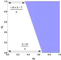
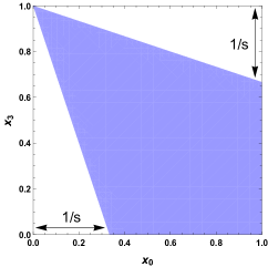
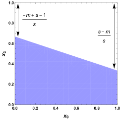
Figure 3: (a) Polygons $\mathcal{P}_{m}$ (shaded areas) for a single symbol, Lagrangian $(x_{0},x_{2})$ plane, exterior letters $m\in\mathcal{A}_{1}$: (left) $m=\underline{1}$, (right) $m=s\!-\!1$. (b) Polygons $\mathcal{P}_{{m_{1}}{m_{2}}}$ (shaded areas) in Lagrangian $(x_{0},x_{3})$ plane for blocks ${m_{1}}{m_{2}}$ of length 2, ${m_{1}}=\underline{1},{m_{2}}=m\in\mathcal{A}_{0}$ (left); ${m_{1}}=\underline{1},{m_{2}}=s-1$ (middle); ${m_{1}}=s-1,{m_{2}}=m\in\mathcal{A}_{0}$ (right). Repeated exterior alphabet symbols are pruned, $\mathcal{P}_{{m}{m}}=\emptyset$ if ${m}\in\mathcal{A}_{1}$. For blocks composed of only interior symbols $m_{1},m_{2}\in\mathcal{A}_{0}$, $\mathcal{P}_{{m_{1}}{m_{2}}}$ is the entire unit square (full shift, no pruning). Note that ${\mu}({{b}})={\mu}({\bar{{b}}})$ by the symmetry (32). Compare also with the state space representation figure 2.

3.5 Evaluation of measures

Since all coefficients in (28) are given by rational numbers, the polygon areas $|\mathcal{P}_{{b}}|$ are rational too. The same holds for the $d_{\ell}$ factor. As a result, measures ${\mu}({{b}})$ are always rational (see, for example, table 1). This allows for their exact evaluation by integer arithmetic. As the factor $d_{\ell}$ in (27) is known explicitly, the evaluation of ${\mu}({b})$ relies on the knowledge of the areas $|\mathcal{P}_{{b}}|$ which can be easily found analytically for small $\ell$. Before working out specific examples, we list symmetry properties of measures ${\mu}({b})$ valid for any block length $\ell$.

Symmetries.

Symmetries of the cat map induce invariance with respect to corresponding symbol exchanges. Define $\bar{m}=s\!-\!2\!-\!m$ to be the conjugate of symbol $m\in\mathcal{A}$. For example, the two exterior alphabet $\mathcal{A}_{1}$ symbols are conjugate to each other, as illustrated by figure 1. If ${b}={m_{1}}{m_{2}}\dots{m_{\ell}}$ is a block, and $\bar{{b}}=\bar{m}_{1}\bar{m}_{2}\dots\bar{m}_{\ell}$ its conjugate, then by reflection symmetry of the cat map we have $|\mathcal{P}_{{b}}|=|\mathcal{P}_{\bar{{b}}}|$. Similarly, if $b^{*}={m_{l}}{m_{l-1}}\dots{m_{1}}$, the time reversal invariance implies $|\mathcal{P}_{{b}}|=|\mathcal{P}_{{b}^{*}}|$. Accordingly, blocks ${b}$, ${b}^{*}$, and $\bar{{b}}$ have the same measure,

$${\mu}({{b}})={\mu}({\bar{{b}}})={\mu}({{b}^{*}})\,.$$ (32)

3.5.1 Example: Measure of blocks of length $\ell=1$.

The defining, single symbol block Lagrangian equation (2) is the simplest example of the Lagrangian, two-point boundary values formulation,

$$x_{1}=\mathsf{g}_{11}{m_{1}}+\mathsf{g}_{11}x_{0}+\mathsf{g}_{11}x_{2}\,,$$

with $\ell=1$, $\mathsf{g}_{11}=1/s$ verifying the general Green’s function formula (24). For single symbol ${m_{1}}\equiv m$ the set of inequalities (28) thus reduces to

$$-m\leq x_{0}+x_{2}<s-m\,.$$

This constraint is always fulfilled for interior symbols $m\in\mathcal{A}_{0}$. For $m\in\mathcal{A}_{1}$, polygon $\mathcal{P}_{m}$ is the upper and lower triangle, respectively, shown in figure 3 (a). As a result, we have $|\mathcal{P}_{m}|=1$ if $m\in\mathcal{A}_{0}$ and $|\mathcal{P}_{m}|=1/2$ if $m\in\mathcal{A}_{1}$, giving measures

$${\mu}(m)=\left\{\begin{array}[]{ll}1/s,&\mbox{for }m\in\mathcal{A}_{0}\\ 1/2s,&\mbox{for }m\in\mathcal{A}_{1}\,,\end{array}\right.$$

which indeed add up to one after summation over all letters of the alphabet $\mathcal{A}$.

3.5.2 Example: Measure of blocks of length $\ell=2$:

For blocks ${m_{1}}{m_{2}}$, bounds (28) give four inequalities

$$-s{m_{1}}-{m_{2}} \leq sx_{0}+x_{3}<s^{2}-1-s{m_{1}}-{m_{2}}$$ (33)

$$-s{m_{2}}-{m_{1}} \leq sx_{3}+x_{0}<s^{2}-1-s{m_{2}}-{m_{1}}\,,$$

where we have used $U_{2}(s/2)=s^{2}-1$. A constraint arises whenever at least one of the symbols belongs to the exterior alphabet $\mathcal{A}_{1}$. By the symmetry (32), it is sufficient to analyze the case when ${m_{1}}=\underline{1}$. If ${m_{2}}\in\mathcal{A}_{0}$, the polygon $\mathcal{P}_{\underline{1}m_{2}}$ is determined by (see figure 3 (b)):

$$s-{m_{2}}\leq sx_{0}+x_{3},\qquad 0\leq x_{0},x_{3}<1.$$

The area of the resulting polygon is equal to $|\mathcal{P}_{\underline{1}m_{2}}|=(1+2m_{2})/2s$, where $m_{2}\in\mathcal{A}_{0}$. If both ${m_{1}}\neq{m_{2}}$ belong to $\mathcal{A}_{1}$, i.e., ${m_{1}}=\underline{1}$, ${m_{2}}=s\!-\!1$, then the corresponding polygon is determined by the conditions:

$$1\leq sx_{0}+x_{3},\qquad sx_{3}+x_{0}\leq s,\qquad 0\leq x_{0},x_{3}<1.$$

with the corresponding area $|\mathcal{P}_{{m_{1}}{m_{2}}}|=1-1/s$. Finally, if both ${m_{1}}={m_{2}}$ belong to $\mathcal{A}_{1}$  and they are equal, then block is pruned, $\mathcal{P}_{{m_{1}}{m_{2}}}=\emptyset$; there are two pruned blocks of length 2. In summary,

$${\mu}({m_{1}}{m_{2}})=\left\{\begin{array}[]{llll}1/s^{2}-1&\mbox{for }{m_{1}},{m_{2}}\in\mathcal{A}_{0}\\ (1+2{m_{2}})/2s(s^{2}-1)&\mbox{for }{m_{1}}=\underline{1},{m_{2}}\in\mathcal{A}_{0}\\ 1/s(s+1)&\mbox{for }{m_{1}}=\underline{1},{m_{2}}=s\!-\!1\\ 0&\mbox{for }{m_{1}}=\underline{1},{m_{2}}=\underline{1}.\end{array}\right.$$ (34)

The measures for the remaining symbol combinations can be obtained by the symmetries, see (32) and table 1 for the $s=3$ case.

3.5.3 Pruning.

As shown in (21), any block of $\mathcal{A}_{0}$ symbols is admissible. If, on the other hand, one or more symbols from ${m}$ belong to $\mathcal{A}_{1}$, such a block might be forbidden, with the polygon $\mathcal{P}_{{m}}$ defined by (28,29) empty, and thus ${\mu}({m})=0$. An example is the pruned blocks $\_{\underline{1}\underline{1}}\_$ and $\_{22}\_$, missing from figure 2 (g). While here we do not attempt to solve the number-theoretic problem of determining the number of pruned blocks for arbitrary $\ell$, the count of pruning rules given in table 2 indicates that for the linear encoding the number of pruned blocks grows exponentially with their length. Thus the linear encoding is not a subshift of finite type, as its grammar consists of an infinity of arbitrarily long pruned (i.e., inadmissible) blocks. While the shaded areas of figure 2 (g-h) are accounted for by the complete Smale-horseshoe grammar of the interior alphabet, the admissibility rules for blocks involving letters from $\mathcal{A}_{1}=\{\underline{1},2\}$ are not known. In [18], an Adler–Weiss Markov generating partition symbolic dynamics for the Percival-Vivaldi cat map (18) is constructed, with complete, finite subshift grammar. That, however, has no bearing on the main thrust of this paper.

Table 2: $N_{n}$ is the total number of pruned blocks of length $n={|b|}$ for the $s=3$ Arnol’d cat map. $\tilde{N}_{n}$ is the number of new pruned blocks of length ${|b|}$, with all length ${|b|}$ blocks that contain shorter pruned blocks already eliminated. Empirically there is a single new pruning rule for each prime-number block length (it is listed as two rules, but by the reflection symmetry there is only one).

$n$ $N_{n}$ $\tilde{N}_{n-1}$ 2 2 0 3 22 2 4 132 8 5 684 2 6 3164 30 7 13894 2 8 58912 70 9 244678 16 10 1002558 198 11 4073528 2 12 16460290 528 13 2

4 Spatiotemporal cat

We now turn to the study of the spatiotemporal cat (4), with cat maps on sites (“particles”) coupled isotropically to their nearest neighbors on a 2-dimensional spatiotemporally infinite $\mathbb{Z}^{2}$ lattice. The coupled map lattices (CML) were introduced in the mid 1980’s as models [32, 33] for studies of spatio-temporal chaos in discretizations of dissipative PDEs. Later on, chains of coupled Anosov maps were investigated in mathematically rigorous settings [13, 43]. The conventional CML models start out with chaotic on-site dynamics weakly coupled to neighboring sites, with strong spacetime asymmetry. In order to establish the desired statistical properties of CML, such as the continuity of their SRB measures, [13, 43] and most of the subsequent mathematical literature rely on the structural stability of Anosov automorphisms under small perturbations. Contrast this with the non-perturbative $2$-dimensional Gutkin-Osipov [29] spatiotemporal cat (4). While this model has a Hamiltonian formulation (see B), as in the cat map case of section 3.1, it is instructive to write down its equations of motion in the Lagrangian form:

$$(-\Box+{2(s-2)})\,x_{z} = {m_{z}}\,,\qquad z=(n,t)\in\mathbb{Z}^{2}\,,$$

$$x_{z}\in[0,1),\quad {m_{z}}\in\mathcal{A}=\{-3,-2,\cdots,{2s}-2,{2s}-1\}\,,$$ (35)

with $\Box$ being the discrete spacetime Laplacian (6) on $\mathbb{Z}^{2}$. The map is space $\leftrightarrow$ time symmetric and has the temporal and spatial dynamics strongly coupled. Furthermore, it is smooth and fully hyperbolic for any integer $|s|>{2}$. In what follows we will assume positive $s>{2}$.

In this paper, we focus on learning how to enumerate admissible spatiotemporal cat spatiotemporal patterns, compute their measures, and identify their recurrences (shadowing of a large invariant 2-torus by smaller invariant 2-tori).

4.1 Linear encoding

The symbols ${m_{z}}$ from the set $\mathcal{A}=\{\underline{3},\underline{2},\cdots,{2s}\!-\!2,{2s}\!-\!1\}$ on the right hand side of (35) are necessary to keep $x_{z}$ within the interval $[0,1)$, with $\underline{m_{z}}$ standing here for $m_{z}$ with the negative sign, i.e., ‘$\underline{3}$’ stands for symbol ‘$-3$’. As we now show, ${\mathsf{M}=\{{m_{z}}\in\mathcal{A}\,,\;z\in\mathbb{Z}^{2}\}}$ can be used as a 2-dimensional symbolic representation (code) of the lattice system states.

Since (35) is a linear equation, any of its solutions $\mathsf{X}=\{x_{z}\in[0,1)\,,\;z\in\mathbb{Z}^{2}\}$ can be uniquely recovered from the corresponding code $\mathsf{M}$. By inverting (35) we obtain

$$x_{z}=\sum_{z^{\prime}\in\mathbb{Z}^{2}}\mathsf{g}_{zz^{\prime}}{m_{z^{\prime}}},\qquad\mathsf{g}_{zz^{\prime}}=\left(\frac{1}{-\Box+{2(s-2)}}\right)_{zz^{\prime}}\,,$$ (36)

where $\mathsf{g}_{zz^{\prime}}$ is the Green’s function for the 2-dimensional discretized heat equation, see A. A symbol block $\mathsf{M}$ is admissible if and only if all $x_{z}$ given by (36) fall into the interval $[0,1)$.

As for the cat map, we split the ${2s}+3$ letter alphabet $\mathcal{A}=\mathcal{A}_{0}\cup\mathcal{A}_{1}$ into the interior $\mathcal{A}_{0}$ and exterior $\mathcal{A}_{1}$ alphabets

$$\mathcal{A}_{0}=\{0,\dots,{2({s}-2)}\},\quad\mathcal{A}_{1}=\{\underline{3},\underline{2},\underline{1}\}\cup\{{2s}\!-\!3,{2s}\!-\!2,{2s}\!-\!1\}\,.$$ (37)

For example, for $s={5/2}$ the interior, respectively exterior alphabets are

$$\mathcal{A}_{0}=\{0,1\},\quad\mathcal{A}_{1}=\{\underline{3},\underline{2},\underline{1}\}\cup\{2,3,4\}\,.$$ (38)

If all ${m_{z}}\in\mathsf{M}$ belong to $\mathcal{A}_{0}$, $\mathsf{M}$ is admissible, i.e., $\mathcal{A}_{0}^{\mathbb{Z}^{2}}$ is a full shift. Indeed, by the positivity of Green’s function (see A) it follows immediately that $0\leq x_{z}$, while the condition $\sum_{z^{\prime}\in\mathbb{Z}^{2}}\mathsf{g}_{zz^{\prime}}={1/2({s}-2)}$ implies that $x_{z}\leq 1$, with the equality saturated only if ${m_{z}}={2({s}-2)}$, for all $z\in\mathbb{Z}^{2}$.

The key advantage of linear encoding is illustrated already by the $d=2$ case. While the size of the alphabet $\bar{\mathcal{A}}$ based on a Markov partition grows exponentially with the “particle number” $L$, the number of letters (4) of the linear encoding $\mathcal{A}$ is finite and the same for any $L$, including the $L\to\infty$ spatiotemporal cat. For the linear encoding an invariant 2-torus is encoded by a doubly periodic $d=2$ block $\mathsf{M}$ of symbols from a small alphabet, rather then by a $1$-dimensional temporal string of symbols from the exponentially large (in $L$) alphabet $\bar{\mathcal{A}}$.

4.2 Finite symbol blocks

Let $\mathcal{R}\subset\mathbb{Z}^{2}$ be a rectangle on $\mathbb{Z}^{2}$ and let ${\mathsf{M}_{\mathcal{R}}}=\{{m_{z}}|z\in\mathcal{R}\}$ be a symbol block defined on $\mathcal{R}$. We now show that ${\mathsf{M}_{\mathcal{R}}}$ determines approximate positions of the points $x_{z}$, $z\in\mathcal{R}$, within the domain $\mathcal{R}$. To start with we define the (exterior) boundary $\partial\mathcal{R}$ of $\mathcal{R}$ as a set of points adjacent to $\mathcal{R}$. More precisely, $z=(n,t)$ belongs to $\partial\mathcal{R}$ if and only if $z\notin\mathcal{R}$ but one of the four neighboring points $(n\pm 1,t)$, $(n,t\pm 1)$ belongs to $\mathcal{R}$, see figure 4(a). Let then $\mathsf{g}_{zz^{\prime}}$ be the corresponding Dirichlet Green’s function which vanishes at the boundary $\partial\mathcal{R}$. By the lattice Green’s identity (see A.3) any solution of the equation (35) satisfies

$$x_{z}=\sum_{z^{\prime}\in\mathcal{R}}\mathsf{g}_{zz^{\prime}}{m_{z^{\prime}}}+\sum_{z^{\prime\prime}\in\partial\mathcal{R}}\mathsf{g}_{z\bar{z}^{\prime\prime}}x_{z^{\prime\prime}}\,,\qquad z\in\mathcal{R}\,,$$ (39)

with $\bar{z}^{\prime\prime}$ being the unique adjacent point of $z^{\prime\prime}\in\partial\mathcal{R}$ within the domain $\mathcal{R}$. Here, the first term

$$\bar{x}_{z}:=\sum_{z^{\prime}\in\mathcal{R}}\mathsf{g}_{zz^{\prime}}{m_{z^{\prime}}}$$ (40)

can be viewed as the “approximate spatiotemporal state” $\bar{x}({\mathsf{M}_{\mathcal{R}}})$ at the point $z$. Importantly, it is determined solely by $\mathsf{M}_{\mathcal{R}}$. From (39) it follows that the difference $|x_{z}-\bar{x}_{z}|$ is bounded by

$$|x_{z}-\bar{x}_{z}|=\sum_{z^{\prime\prime}\in\partial\mathcal{R}}\mathsf{g}_{z\bar{z}^{\prime\prime}}x_{z^{\prime\prime}}\leq|\partial\mathcal{R}|\,\mathsf{g}_{z\bar{z}^{\prime\prime}_{0}}\,,$$

with $\bar{z}^{\prime\prime}_{0}$ being the boundary point of $\mathcal{R}$ (i.e., adjacent to $\partial\mathcal{R}$), where the function $\mathsf{g}_{z\bar{z}^{\prime\prime}}$ attains its maximum value along $\partial\mathcal{R}$ (for a fixed $z$). For an illustration, consider a $[\ell_{1}\!\times\!\ell_{2}]$ rectangular domain

$$\mathcal{R}^{[\ell_{1}\times\ell_{2}]}=\{(i,j)|\,i=0,\cdots,\ell_{1}\!-\!1,\;j=0,\cdots,\ell_{2}\!-\!1\}\,,$$ (41)

with $\ell_{1}$, $\ell_{2}$ even (see figure 4 (a)), and take the point $z$ at the rectangular center. As the Green’s function $\mathsf{g}_{z\bar{z}^{\prime\prime}}$ decays exponentially with $|z-\bar{z}^{\prime\prime}|$ (see A.2), the distance $|x_{z}-\bar{x}_{z}|$ is of the order $e^{-\nu\ell_{\min}}$ for a large $\ell_{\min}=\min{\{\ell_{1}/2,\ell_{2}/2\}}$, where the exponent $\nu$ is defined by $\cosh\nu=s/{2}$.

We determine next the measure ${\mu}({\mathsf{M}_{\mathcal{R}}})$ of the cylinder set corresponding to ${\mathsf{M}_{\mathcal{R}}}$. Take $\mathcal{R}=\mathcal{R}^{[\ell_{1}\times\ell_{2}]}$ to be a rectangular domain (41). In what follows it is convenient to distinguish points in the interior of $\mathcal{R}$  from the points which belong to the boundary $\partial\mathcal{R}$. While in principle the boundary state space points $x_{z^{\prime\prime}}\in\partial\mathcal{R}$ are labelled by the symbol pair $z^{\prime\prime}=(n,t)$, we find it more convenient to label them by a single index that indicates their position along the border, $x_{i}=x_{z^{\prime\prime}}$, where $i$ runs from $1$ to ${|\partial\mathcal{R}|}=2(\ell_{1}+\ell_{2})$. For examples, see figure 4 and sections 4.3.1 and 4.3.2. Both the boundary state space points $x_{i},i=1,\dots{|\partial\mathcal{R}|}$ and the internal points $x_{z},z\in\mathcal{R}$ must lie within the unit interval.

Theorem 4.1.

Given a block of symbols ${\mathsf{M}_{\mathcal{R}}}$ on rectangle $\mathcal{R}$, the measure ${\mu}({\mathsf{M}_{\mathcal{R}}})$ can be factorized into product

$${\mu}({\mathsf{M}_{\mathcal{R}}})=d(\mathcal{R})\,|\mathcal{P}({\mathsf{M}_{\mathcal{R}}})|\,,$$ (42)

where $|\mathcal{P}({\mathsf{M}_{\mathcal{R}}})|$ is the volume of the ${|\partial\mathcal{R}|}$-dimensional polytope $\mathcal{P}({\mathsf{M}_{\mathcal{R}}})$, defined by the following inequalities

$$0 \leq x_{i}<1,\qquad i=1,\dots,{|\partial\mathcal{R}|}\,,$$ (43)

$$0 \leq\bar{x}_{z}+\sum_{i=1}^{|\partial\mathcal{R}|}\mathsf{g}_{z\bar{z}_{i}}x_{i}<1,\qquad z\in\mathcal{R}\,$$ (44)

and the factor $d(\mathcal{R})$ depends only on the sizes $\ell_{1},\ell_{2}$ of $\mathcal{R}$, but not on the symbolic content of ${\mathsf{M}_{\mathcal{R}}}$.

Proof.

Since for all interior points $z\in\mathcal{R}$ one has $0\leq x_{z}<1$, (39) implies that the admissible set of boundary points $x_{i},i=1,\dots,{|\partial\mathcal{R}|}$ satisfy inequalities (43) and (44). Essentially, the inequalities (44) cut out the polytope $\mathcal{P}({\mathsf{M}_{\mathcal{R}}})$ out of the ${|\partial\mathcal{R}|}$-dimensional unit hypercube defined by (43). As a result, the measure ${\mu}({\mathsf{M}_{\mathcal{R}}})$ is given by the product of the $\mathcal{P}({\mathsf{M}_{\mathcal{R}}})$ volume and the Jacobian $d(\mathcal{R})$ of the linear transformation between boundary coordinates (43) and the set of $2(\ell_{1}+\ell_{2})$ coordinates

$$\{(x_{nt_{0}},x_{nt_{1}})\,|\,n=-\lfloor\ell_{2}/2\rfloor,\dots,-\lfloor\ell_{2}/2\rfloor+\ell_{1}+\ell_{2}-2\}$$

at the two consecutive times $t_{0}=\lfloor\ell_{1}/2\rfloor$, $t_{1}=t_{0}+1$. Since the Jacobian of this transformation is independent of any particular block ${\mathsf{M}_{\mathcal{R}}}$, the factor $d(\mathcal{R})$ depends only on $\mathcal{R}$, but not on its symbolic content. ∎

As was the case for the single cat map theorem 3.1, the theorem yields a simple result for symbol blocks composed only of the interior alphabet symbols:

Corollary 4.1.1.

If all symbols in ${\mathsf{M}_{\mathcal{R}}}$ belong to the interior alphabet $\mathcal{A}_{0}$ (37), then

$${\mu}({\mathsf{M}_{\mathcal{R}}})={d(\mathcal{R})}$$ (45)

is independent of the symbolic content of ${\mathsf{M}_{\mathcal{R}}}$.

Proof.

Note that the inequalities (44) are satisfied if all symbols from ${\mathsf{M}_{\mathcal{R}}}$ belong to the interior alphabet $\mathcal{A}_{0}$ (37). This follows from the positivity of the Green’s function $\mathsf{g}_{zz^{\prime}}$, and the identity

$$1=2(s-2)\sum_{z^{\prime}\in\mathcal{R}}\mathsf{g}_{zz^{\prime}}+\sum_{z^{\prime\prime}\in\partial\mathcal{R}}\mathsf{g}_{z\bar{z}^{\prime\prime}},\qquad z\in\mathcal{R}\,,$$

obtained by substituting the spatiotemporal cat (35) constant field solution $x_{z}=1$, ${m_{z}}=2(s-2)$ into the Green’s function (39) - see discussion following (38). As a result, for any block ${\mathsf{M}_{\mathcal{R}}}$ of interior symbols $\mathcal{P}({{\mathsf{M}_{\mathcal{R}}}})$ is just a hypercube with $|\mathcal{P}({{\mathsf{M}_{\mathcal{R}}}})|=1$, and (45) follows immediately. ∎

4.3 Evaluation of measures

The evaluation of measures ${\mu}({\mathsf{M}_{\mathcal{R}}})$ for the spatiotemporal cat  boils down to the evaluation of the polytope volumes $|\mathcal{P}({{\mathsf{M}_{\mathcal{R}}}})|$, determined by the inequalities (43) and (44). By the rationality of every element $\mathsf{g}_{zz^{\prime}}$, $|\mathcal{P}({{\mathsf{M}_{\mathcal{R}}}})|$ is given by a rational number for any ${\mathsf{M}_{\mathcal{R}}}$. This allows for exact evaluation of $|\mathcal{P}({{\mathsf{M}_{\mathcal{R}}}})|$ by integer arithmetic. Once the volumes are found for all admissible blocks ${\mathsf{M}_{\mathcal{R}}}$, the constant factor $d(\mathcal{R})$ can be extracted from the normalization condition, by summing up all volumes:

$$1/d(\mathcal{R})=\sum|\mathcal{P}({{\mathsf{M}_{\mathcal{R}}}})|\,.$$ (46)

We were unable to derive any explicit formulas for $d(\mathcal{R})$. However, its asymptotic form in the limit of large domains can be related to the spatiotemporal metric entropy, as discussed in C.2.

Before looking at specific examples of measure calculation we list the symmetry properties of the spatiotemporal cat measures ${\mu}({\mathsf{M}_{\mathcal{R}}})$.

Symmetries.

Besides the invariance under shifts in time and space directions, spatiotemporal cat (35) is separately invariant under the space and time reflections $n\to-n$, $t\to-t$, as well as under exchange $n\longleftrightarrow t$ of space and time. Spatiotemporal cat thus has all the symmetries of the square lattice:

• 2 discrete translation symmetries

• the group $D_{4}$ composed of rotations by $k\pi/2$, $k=1,2,3$ and reflection across $x$-axis, $y$-axis, diagonal $a$, diagonal $b$:

  $$C_{4v}=\textrm{D}_{4}=\{E,C_{4z}^{+},C_{4z}^{-},C_{2z},\sigma_{y},\sigma_{x},\sigma_{da},\sigma_{db},\}\,.$$ (47)

In the international crystallographic notation [22], this point group is referred to as $p4mm$. In addition, the transformation

$$x_{nt}\to 1-x_{nt},\qquad\mathsf{M}=\{{m_{nt}}\}\to\bar{\mathsf{M}}=\{\bar{m}_{nt}\},\quad\bar{m}_{nt}={2(s-2)}-{m_{nt}}\,,$$

leaves eq. (35) invariant. All together, the measure is invariant under

$${\mu}({\mathsf{M}_{\mathcal{R}}})={\mu}(\sigma\circ{\mathsf{M}_{\mathcal{R}}}),\qquad{\mu}({\mathsf{M}_{\mathcal{R}}})={\mu}(\bar{\mathsf{M}}_{\mathcal{R}}),$$

where $\sigma$ is an element of space group $p4mm$. As an example, consider ${s=7/2}$ spatiotemporal cat, with alphabets (37)

$$\mathcal{A}_{0}=\{0,1,2,3\},\quad\mathcal{A}_{1}=\{\underline{3},\underline{2},\underline{1}\}\cup\{4,5,6\}\,.$$ (48)

By the $\textrm{D}_{4}$ symmetries ${\mu}({\mathsf{M}_{\mathcal{R}}})={\mu}(\sigma\circ{\mathsf{M}_{\mathcal{R}}})$ the measures of the following eight blocks are equal:

$$\left[\begin{array}[]{cc}1&2\\ 3&4\\ 5&6\end{array}\right],\qquad\left[\begin{array}[]{ccc}2&4&6\\ 1&3&5\end{array}\right],\qquad\left[\begin{array}[]{cc}6&5\\ 4&3\\ 2&1\end{array}\right],\qquad\left[\begin{array}[]{ccc}5&3&1\\ 6&4&2\end{array}\right]$$

$$\left[\begin{array}[]{cc}2&1\\ 4&3\\ 6&5\end{array}\right],\qquad\left[\begin{array}[]{ccc}6&4&2\\ 5&3&1\end{array}\right],\qquad\left[\begin{array}[]{cc}5&6\\ 3&4\\ 1&2\end{array}\right],\qquad\left[\begin{array}[]{ccc}1&3&5\\ 2&4&6\end{array}\right]\,.$$

In addition, the measures of blocks such as

$$\left[\begin{array}[]{cc}2&1\\ 4&3\\ 6&5\end{array}\right]\quad\Leftrightarrow\quad\left[\begin{array}[]{cc}1&2\\ \underline{1}&0\\ \underline{3}&\underline{2}\end{array}\right]$$

(eight additional blocks in all) are equal by ${\mu}({\mathsf{M}_{\mathcal{R}}})={\mu}(\bar{\mathsf{M}}_{\mathcal{R}})$ symmetry.

While for a cat map ${|\partial\mathcal{R}|}$ is always $2$, i.e., the boundary of interval $\mathcal{R}$ consists of the two end points, for the spatiotemporal cat the number ${|\partial\mathcal{R}|}$ of boundary points grows with the domain size. The complexity of $|\mathcal{P}({{\mathsf{M}_{\mathcal{R}}}})|$ calculation for a spatiotemporal cat thus grows with $|\mathcal{R}|$, as well. We illustrate this with calculations for $\mathcal{R}=[1\!\times\!1]$ and $[2\!\times\!2]$ symbol blocks.

4.3.1 Example: $\mathcal{R}=[1\!\times\!1]$ measure.

Consider a $\mathcal{R}=[1\!\times\!1]$ spatiotemporal domain, with a single symbol block $\mathsf{M}$, together with the four state space points $x_{i}=x_{z}\in\partial\mathcal{R}$ comprising its boundary, figure 4 (b). We need to evaluate the volume of the 4-dimensional polytope $\mathcal{P}(m)$ for each $m\in\mathcal{A}$. $\mathcal{P}(m)$ is contained with the hypercube

$$0\leq x_{i}<1,\qquad i=1,2,3,4,$$

bounded by the inequalities

$$-m\leq x_{1}+x_{2}+x_{3}+x_{4}<{2s}-m\,.$$ (49)

The polytope volume $|\mathcal{P}(m)|$ depends on $m$. For the interior letters $m\in\mathcal{A}_{0}$ the hyperplane (49) does not intersect the hypercube and the volume $|\mathcal{P}(m)|=1$. For $m\in\{\underline{3},\underline{2},\underline{1}\}$ in the exterior $\mathcal{A}_{1}$ alphabet (37), the corresponding volumes $|\mathcal{P}(m)|$ are $1/4!$, $1/2$, and $23/4!$, respectively. The normalization condition (46) then yields $d=1/(2s)$. Thus the measures for the symbols from the exterior alphabet $\mathcal{A}_{1}$ are

$${\mu}(\underline{3}) = {\mu}({2s\!-\!1})={1}/{{(2\cdot 4!\,s)}}$$

$${\mu}(\underline{2}) = {\mu}({2s}\!-\!2)={1}/{(4s)}$$

$${\mu}(\underline{1}) = {\mu}({2s\!-\!3})={1}/{(2s)}-{1}/{{(2\cdot 4!\,s)}}$$

$${\mu}(m) = {1}/{{2s}}\mbox{ for the }{2s-3}\mbox{ interior letters }m\in\mathcal{A}_{0}\,,$$ (50)

with the total measure satisfying $\sum_{{m}}{\mu}({m})=1\,.$ The numerical estimates of figure 5 confirm these analytic results.

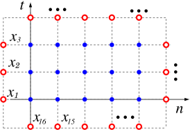
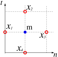
(a)     (b)     (c) 

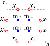
Figure 4: (Color online) (a) A $[5\!\times\!3]$ domain $\mathcal{R}$ on the 2-dimensional lattice. The red (open) circles indicate the boundary $\partial\mathcal{R}$. For each point $x_{i}\in\partial\mathcal{R}$, there exists a unique adjacent point within the domain $\mathcal{R}$. Blocks ${\mathsf{M}_{\mathcal{R}}}$ for (b) $\mathcal{R}=[1\!\times\!1]$, and (c) $\mathcal{R}=[2\!\times\!2]$ domains, together with the corresponding boundary points $\partial\mathcal{R}=\{x_{1},x_{2},x_{3},x_{4}\}$ and $\partial\mathcal{R}=\{x_{1},x_{2},\cdots,x_{8}\}$, respectively.

4.3.2 Example: $\mathcal{R}=[2\!\times\!2]$ measure.

For the block

$$\mathsf{M}=\left[\begin{array}[]{c}{m_{12}}{m_{22}}\\ {m_{11}}{m_{21}}\end{array}\right]$$ (51)

the 8-dimensional polytope $\mathcal{P}_{\mathsf{M}}$ is parametrized by the boundary $\partial\mathcal{R}$ points, figure 4 (c). They satisfy $0\leq x_{i}<1,i=1,\dots 8$, supplemented by the four inequalities:

$$0<P_{k}(x_{1},\dots,x_{8})\leq{8\,s(s^{2}-1)},\qquad k=1,2,3,4,$$ (52)

where

$$P_{1}={2(2s^{2}-1)}(x_{1}+x_{8}+{m_{11}})+{2s}(x_{3}+x_{2}+x_{6}+x_{7}+{m_{12}}+{m_{21}})+2(x_{4}+x_{5}+{m_{22}})$$

$$P_{2}={2(2s^{2}-1)}(x_{2}+x_{3}+{m_{12}})+{2s}(x_{1}+x_{8}+x_{4}+x_{5}+{m_{11}}+{m_{22}})+2(x_{7}+x_{6}+{m_{21}})$$

$$P_{3}={2(2s^{2}-1)}(x_{7}+x_{6}+{m_{21}})+{2s}(x_{1}+x_{8}+x_{4}+x_{5}+{m_{22}}+{m_{11}})+2(x_{2}+x_{3}+{m_{12}})$$

$$P_{4}={2(2s^{2}-1)}(x_{4}+x_{5}+{m_{22}})+{2s}(x_{3}+x_{2}+x_{6}+x_{7}+{m_{12}}+{m_{21}})+2(x_{1}+x_{8}+{m_{11}})\,.$$

These inequalities lead to analytical expressions for $\mathcal{P}_{\mathsf{M}}$ volumes. A general $\mathcal{P}_{\mathsf{M}}$ volume is a four-dimensional integral, whose calculation is lengthy and unilluminating, so we skip it here. Instead, we evaluate $|\mathcal{P}_{\mathsf{M}}|$ for cases where some of the inequalities (52) are satisfied for all points of the hypercube $\mathcal{P}_{0}=\{x_{1},\dots,x_{8}\in[0,1)\}$. If all letters of $\mathsf{M}$ belong to the interior alphabet, then all inequalities hold, and $|\mathcal{P}_{\mathsf{M}}|=1$. Another easy case is the one where three out of four inequalities hold for all points in $\mathcal{P}_{0}$. For example, consider

$$\mathsf{M}=\left[\begin{array}[]{cc}{s}-2&{s}-2\\ \underline{2}&{s}-1\end{array}\right]$$

for an even ${s>2}$. Then only the first inequality, $0<P_{1}(x_{1},\dots,x_{8})$, is a non-trivial one, while the rest are satisfied for all points in $\mathcal{P}_{0}$. Since the center of the hypercube $\{x_{i}=1/2,i=1,\dots,8\}$ belongs to the hyperplane $P_{1}(x_{1},\dots,x_{8})=0$, the polytope $\mathcal{P}_{\mathsf{M}}$ has the same volume as half of the hypercube $\mathcal{P}_{0}$, i.e., $|\mathcal{P}_{\mathsf{M}}|=1/2$.

It is also possible to find all inadmissible symbol blocks, with $|\mathcal{P}_{\mathsf{M}}|=0$. For inadmissible symbol blocks, one of the inequalities (52) must be violated for all points of the hypercube $\mathcal{P}_{0}$. In particular, any combination of symbols for $[2\!\times\!2]$ block that satisfies condition

$$(2+{m_{11}}){(2s^{2}-1)}+(4+{m_{12}}+{m_{21}}){s}+(2+{m_{22}})\leq 0$$

is forbidden, i.e., $|\mathcal{P}_{\mathsf{M}}|=0$. This implies that symbol blocks

$$\left[\begin{array}[]{cc}\underline{2}&\underline{2}\\ \underline{2}&\underline{2}\end{array}\right],\qquad\left[\begin{array}[]{cc}{m_{12}}&{m_{22}}\\ \underline{3}&{m_{21}}\end{array}\right]$$

are inadmissible if either ${m_{12}}+{m_{21}}\leq{2s}-6$ and arbitrary ${m_{22}}$, or ${m_{12}}+{m_{21}}={2s}-5,{m_{22}}\leq{s}-3$. Other forbidden $[2\times 2]$ blocks are obtained by application of the symmetry operations.

4.3.3 Numerics.

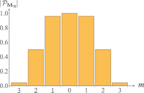
(a)       (b) 

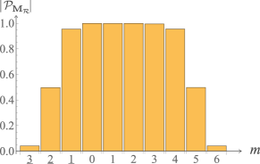
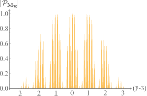
(c)       (d) 

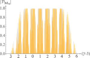
Figure 5: Relative frequencies $|\mathcal{P}_{\mathsf{M}_{\mathcal{R}}}|=f({\mathsf{M}_{\mathcal{R}}})/{d_{\mathcal{R}}}$ of blocks ${\mathsf{M}_{\mathcal{R}}}$ obtained from long-time numerical simulations ($\sim 10^{7}$ iterations, rounded off to two significant digits) are in agreement with the exact formulas of (50). (a) $\mathcal{R}=[1\!\times\!1]$ domain, figure 4 (b), ${s=2}$. The interior alphabet (37) consists of only one letter $\mathcal{A}_{0}=\{0\}$, with the corresponding polytope of maximal volume, $|\mathcal{P}(0)|=1$. (b) $\mathcal{R}=[1\!\times\!1]$, ${s=7/2}$. The maximum frequencies are attained for the four letters (48) from the interior alphabet $\mathcal{A}_{0}=\{0,1,2,3\}$. The blocks ${\mathsf{M}_{\mathcal{R}}}$ over the $\mathcal{R}=[2\!\times\!2]$ spatiotemporal domain, figure 4 (c), can be represented as numbers (53) in base ${2s}+3$. (c) For $\mathcal{R}=[2\!\times\!2]$, ${s}=2$, the only combination of interior symbols that attains the maximum measure is ${m_{11}}={m_{12}}={m_{21}}={m_{22}}=0$. (d) For $\mathcal{R}=[2\!\times\!2]$, ${s=7/2}$, the interior alphabet $\mathcal{A}_{0}$ (48) has $4$ letters, so there are $4^{4}$ blocks that attain the maximum measure.

The volumes of $\mathcal{P}_{\mathsf{M}}$ evaluated analytically are found to be consistent with the measure of a given block $\mathsf{M}$ obtained by numerical simulations of trajectories with random initial conditions.

While in the $\mathcal{R}=[1\!\times\!1]$ case it was possible to plot the single symbol block $\mathsf{M}$ measures ${\mu}({m_{j}})$ along a single, integer $j$ labelled axis, as in figure 5 (a) and (b), the $\mathcal{R}=[2\!\times\!2]$ has four sites $z\in\{11,12,21,22\}\,.$ A way to map the array (51) onto a line is to write it as

$$\gamma({\mathsf{M}_{\mathcal{R}}})=\gamma_{1}.\gamma_{2}\gamma_{3}\gamma_{4}$$ (53)

in base ${2s}+3$, where $\gamma_{k}\in\{0,1,\cdots,{2s}+2\}$ are the symbols ${m_{ij}}$ shifted into nonnegative integers,

$$(\gamma_{1},\gamma_{2},\gamma_{3},\gamma_{4})=({m_{11}}+3,{m_{12}}+3,{m_{21}}+3,{m_{22}}+3)\,.$$

Estimates of the corresponding measures ${\mu}({\mathsf{M}_{\mathcal{R}}})$ from long-time numerical Hamiltonian simulations, on a spatially periodic domain of extent $L=20$, are displayed in this way in figure 5 (c) and (d), and are in full agreement with the available analytical data. In particular, whenever all symbols ${m_{ij}}$ belong to the interior alphabet, the numerics is consistent with relative frequency $|\mathcal{P}_{{\mathsf{M}_{\mathcal{R}}}}|=1$.

5 Families of invariant 2-tori

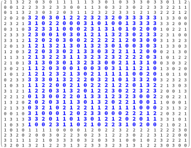
(a) (b)

Figure 6: (Color online) Blocks $\mathsf{M}$, $\mathsf{M}^{\prime}$ encoding two $[L\!\times\!T]=[28\times 27]$ invariant 2-tori $\mathsf{X}$, $\mathsf{X}^{\prime}$ that shadow each other within the $[19\times 20]$ domain $\mathcal{R}\subset\mathcal{R}_{\scriptscriptstyle\mathrm{LT}}$ (bold/blue). The symbols over the $\mathcal{R}$ are drawn randomly from the ${s=7/2}$ interior alphabet $\mathcal{A}_{0}=\{0,1,2,3\}$ and are the same for both symbolic blocks $\mathsf{M}$, $\mathsf{M}^{\prime}$. The symbols outside $\mathcal{R}$, also drawn randomly from $\mathcal{A}_{0}$, differ for $\mathsf{M}$, $\mathsf{M}^{\prime}$.

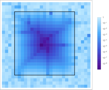
(a) (b)

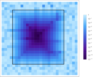
Figure 7: (Color online) The plots of the logarithm of the site-wise distance $|x_{z}-x^{\prime}_{z}|$ of the states $\mathsf{X}$, $\mathsf{X}^{\prime}$ of figure 6 for (a) ${s=7/2}$ and (b) ${s=13/2}$ illustrate the exponential fall-off of the site-wise distances as one approaches the center of the shared symbol domain ${\mathcal{R}}$. The exponential fall-off towards the center of ${\mathcal{R}}$ is faster for $s=13$. Outside of the shared domain $\mathcal{R}$ the distances are of the order $1$.

Linear encoding makes it an easy task to obtain spatiotemporal cat (35) solutions. Of particular interest are the doubly periodic solutions (the spatiotemporal analogs of $d\!=\!1$ cat map periodic orbits), the invariant 2-tori with periods $L$ and $T$,

$$x_{nt}=x_{n+L,t+T},\qquad n=1,\cdots,L,\;\;t=1,\cdots,T\,,$$

invariant under spatial $\mathcal{S}^{L}$ and temporal $\mathcal{T}^{T}$ shifts.

Since the interior alphabet $\mathcal{A}_{0}$ corresponds to a full shift dynamical system, any $[L\!\times\!T]$ block of interior symbols $\mathsf{M}=\{{m_{z}}\in\mathcal{A}_{0}|z\in\mathcal{R}_{\scriptscriptstyle\mathrm{LT}}\}$ over the rectangular spatiotemporal domain

$$\mathcal{R}_{\scriptscriptstyle\mathrm{LT}}=\{z=(n,t)|n=1,\cdots,L,\;\;t=1,\cdots,T\}\,,$$

is admissible and generates an invariant 2-torus solution of (35). The corresponding spatiotemporal state $\mathsf{X}=\{x_{z},z\in\mathcal{R}_{\scriptscriptstyle\mathrm{LT}}\}$ (restricted to the domain $\mathcal{R}_{\scriptscriptstyle\mathrm{LT}}$) is obtained by taking the inverse of (35):

$$x_{z}=\sum_{z^{\prime}\in\mathcal{R}_{\scriptscriptstyle\mathrm{LT}}}\mathsf{g}^{0}_{zz^{\prime}}{m_{z^{\prime}}},\qquad{m_{z^{\prime}}}\in\mathcal{A}_{0}\,,$$ (54)

where $\mathsf{g}^{0}_{zz^{\prime}}$ is the Green’s function with periodic boundary conditions, see  [18]. We next use the obtained solutions to test shadowing properties of invariant 2-tori.

5.1 Partial shadowing

As the first application, we show in figure 6 two $[L\!\times\!T]$ blocks $\mathsf{M}$, $\mathsf{M}^{\prime}$ composed of interior symbols $m_{z}\in\mathcal{A}_{0}$, which coincide within a rectangular domain $\mathcal{R}\subset\mathcal{R}_{\scriptscriptstyle\mathrm{LT}}$. In figure 7, we show the distances between the corresponding spatiotemporal states $\mathsf{X}$, $\mathsf{X}^{\prime}$. In agreement with the results of section 4.2, the distances between $x_{z}\in\mathsf{X}$ and $x_{z}^{\prime}\in\mathsf{X}^{\prime}$ shrink exponentially as $z$ approaches the center of the domain $\mathcal{R}$. In other words, $\mathsf{X}$ and $\mathsf{X}^{\prime}$ shadow each other within the domain $\mathcal{R}$.

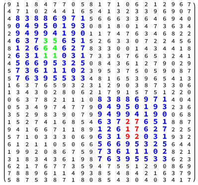
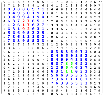
Figure 8: (Color online) Symbol blocks $\mathsf{M}_{1}$, $\mathsf{M}_{2}$ of two $[25\times 25]$ invariant 2-tori $\mathsf{X}_{1}$, $\mathsf{X}_{2}$, with annular (encounter) domains $\mathcal{R}_{1}$ and $\mathcal{R}_{2}$ indicated in blue (bold). The symbols are drawn randomly from the interior alphabet $\mathcal{A}_{0}$ for ${s=13/2}$. The two blocks $\mathsf{M}_{1}$, $\mathsf{M}_{2}$ are related by the permutation of symbol blocks over the interior domains $A_{1}$, $A_{2}$ (red and green, respectively). Any $[3\times 3]$ symbol block $\mathsf{M}^{[3\times 3]}$ appears the same number of times in both $\mathsf{M}_{1}$ and $\mathsf{M}_{2}$, and the two invariant 2-tori $\mathsf{X}_{1}$ and $\mathsf{X}_{2}$ shadow each other at every point.

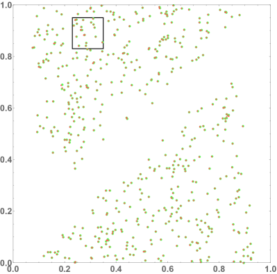
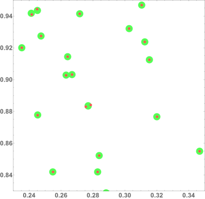
Figure 9: (Color online) (left) Hamiltonian coordinate-momentum representation of the two invariant 2-tori $\mathsf{X}_{1},\mathsf{X}_{2}$ of figure 8. This Hamiltonian representation is explained in B. (right) An enlargement of the square in (left). The small (red) circles indicate points $(q^{(1)}_{z},p^{(1)}_{z})$ of $\mathsf{X}_{1}$. The large (green) circles correspond to the points $(q^{(2)}_{z},p^{(2)}_{z})$ of $\mathsf{X}_{2}$. The solutions pair nearly perfectly, except for the points from the encounter domains $z\in\mathcal{R}_{1}\cup\mathcal{R}_{2}$, where some small deviations can be observed.

5.2 Full shadowing

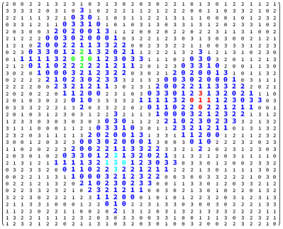
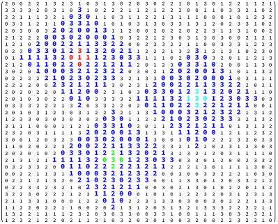
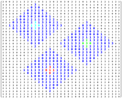
Figure 10: (Color online) Symbol blocks $\mathsf{M}_{1},\mathsf{M}_{2},\mathsf{M}_{3}$ of three $[33\times 33]$ invariant 2-tori $\mathsf{X}_{1},\mathsf{X}_{2},\mathsf{X}_{3}$, with the 3-encounter diamond-shaped domains $\mathcal{R}_{1},\mathcal{R}_{2},\mathcal{R}_{3}$ indicated in blue (bold). The symbols are drawn randomly from the interior alphabet $\mathcal{A}_{0}$ for ${s=7/2}$. $\mathsf{M}_{1}\to\mathsf{M}_{2}\to\mathsf{M}_{3}$ are related by the cyclic permutation of the symbol blocks within the interior domains (red, green, light blue). Any distinct $[4\!\times\!4]$ symbol block $\mathsf{M}^{[4\times 4]}$ appears the same number of times in each invariant 2-torus (or not at all).

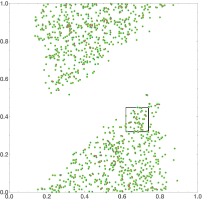
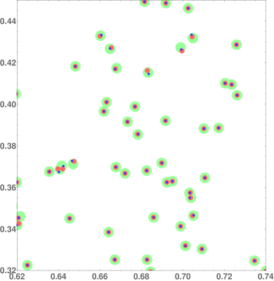
Figure 11: (Color online) (left) Hamiltonian coordinate-momentum representation $(q^{(i)}_{z},p^{(i)}_{z})$, $i=1,2,3$ of the three invariant 2-tori  $\mathsf{X}_{i}$, $i=1,2,3$ of figure 10, shown as centers of the green, red and blue circles. (right) An enlargement of the (left) state space. Note that the three invariant 2-tori $\mathsf{X}_{i}$ form almost perfect triplets except for the points from the encounter domains, $z\in\mathcal{R}_{1}\cup\mathcal{R}_{2}\cup\mathcal{R}_{3}$ where some deviations can be observed.

The invariant 2-tori $\mathsf{X}$ and $\mathsf{X}^{\prime}$ of the above example shadow each other only partially - outside of the subdomain $\mathcal{R}$ their points are not paired. On the other hand, it turns out to be possible to find different invariant 2-tori solutions of (35) which shadow each other at every point of $\mathcal{R}_{\scriptscriptstyle\mathrm{LT}}$. Such solutions, referred as partners, play an important role in the semiclassical treatment of the corresponding quantum problem, since their action differences are small, see [45, 39, 28, 27, 29]. We briefly recall here the construction of partner solutions in $d=2$ setting, following [29].

Let $\{\mathcal{R}_{1},\dots,\mathcal{R}_{m}\},\;\mathcal{R}_{j}\subset\mathcal{R}$, be ${m}$ non-overlapping domains obtained by spacetime shifts $(n,t)\to(n+n_{i},t+t_{i},)$, $i=2,\dots{m}$ of a given domain $\mathcal{R}_{1}$,

$$\mathcal{R}_{i}=\mathcal{S}^{n_{i}}\mathcal{T}^{t_{i}}\,\mathcal{R}_{1}\,,\qquad\mathcal{R}_{i}\cap\mathcal{R}_{j}=\emptyset\mbox{ for }i\neq j\,.$$

Examples of such domains (referred to as “${m}$-encounters”) are given in figures 8 and 10. Assume that the domain $\mathcal{R}_{1}$ has an annular shape with a non-empty interior $A_{1}$, and an exterior $C_{1}=\mathcal{R}_{\scriptscriptstyle\mathrm{LT}}\setminus{A}_{1}\cup\mathcal{R}_{1}$. We define the width $\ell$ of “annulus” $\mathcal{R}_{1}$ by determining the largest $[\ell\!\times\!\ell]$ square domain $\mathcal{R}^{[\ell\times\ell]}$ that can fit into $\mathcal{R}_{1}$ i.e., $\mathcal{R}^{[\ell\times\ell]}$ that has no simultaneous intersections with both the hole and the exterior. In other words, $\ell$ is the maximum integer such that either $A_{1}\cap\mathcal{R}^{[\ell\times\ell]}=\emptyset$, or $C_{1}\cap\mathcal{R}^{[\ell\times\ell]}=\emptyset$, for any translation of $\mathcal{R}^{[\ell\times\ell]}$. All encounter domains $\mathcal{R}_{i}$ have the same width $\ell$, as they are translations of each other.

Now, let block $\mathsf{M}\equiv\mathsf{M}_{1}=\{{m_{z}}\in\mathcal{A}_{0}|z\in\mathcal{R}\}$ be a $[L\!\times\!T]$ symbolic representation of a spatiotemporal cat (35) invariant 2-torus state $\mathsf{X}\equiv\mathsf{X}_{1}$, such that it contains the same block of symbols over each of the subdomains $\mathcal{R}_{1},\dots,\mathcal{R}_{m}$,

$$\mathsf{M}_{\mathcal{R}_{1}}=\mathsf{M}_{\mathcal{R}_{2}}=\dots=\mathsf{M}_{\mathcal{R}_{m}}\,,$$

where $\mathsf{M}_{\mathcal{R}_{i}}$ stands for the restriction of $\mathsf{M}$ to the domain $\mathcal{R}_{i}$. Provided that the $m$ interior domains $A_{1},\dots A_{m}$ have different symbolic content, $\mathsf{M}_{A_{i}}\neq\mathsf{M}_{A_{j}}$ for $i\neq{j}$, we can generate $m!$ distinct blocks $\mathsf{M}_{a},a=1,\dots m!$ by permuting symbol blocks $\mathsf{M}_{A_{i}}$ over the domains $A_{1},\dots A_{m}$. This leads to ${m}!$ distinct invariant 2-tori $\mathsf{X}_{1},\dots\mathsf{X}_{{m}!}$ whose symbol blocks $\mathsf{M}_{1},\dots\mathsf{M}_{{m}!}$ share the following property: each distinct $[\ell\!\times\!\ell]$ square symbol block appears one and the same number of times in all $\mathsf{M}_{a},\,a=1,\dots,m!$, with $\ell$ being the width of the encounter domains $\mathcal{R}_{i}$. In other words, if a $[\ell\!\times\!\ell]$ symbol block $\mathsf{M}^{[\ell\times\ell]}$ appears in $\mathsf{M}_{1}$ a number of times (or zero times), it must appear the same number of times in the encoding $\mathsf{M}_{a}$ of any other invariant 2-torus $\mathsf{X}_{a},a\neq 1$.

By the shadowing property, this in turn implies that all $\mathsf{X}_{1},\dots\mathsf{X}_{{m}!}$ pass through approximately the same points of the state space but in a different spatiotemporal ‘order’. The degree of their closeness is controlled by the parameter $\ell$. The larger $\ell$ is, the closer two different $\mathsf{X}_{a}$, $\mathsf{X}_{b}$ come to each other in the state space. In figures 9 and 11 we illustrate these pairings for families of invariant 2-torus solutions which symbolic representations are shown in figures 8 and 10, respectively.

6 Summary and discussion

In this paper, we have analyzed the spatiotemporal cat (4) linear encoding. We now summarize our main findings.

The finite alphabet of symbols $\mathcal{A}$ encoding system’s dynamics has been shown to split into interior $\mathcal{A}_{0}$ and exterior $\mathcal{A}_{1}$ parts, where only symbolic blocks containing external symbols require non-trivial grammar rules. Blocks composed of only interior symbols are admissible and attain one and the same measure for a given domain $\mathcal{R}$. Furthermore, the measure of a general block factorizes into product of a constant factor $d_{\mathcal{R}}$ and the geometric one $|\mathcal{P}_{\mathcal{R}}|$ which can be interpreted as a volume of certain type of polytope in the Euclidean space whose dimension is determined by the length of the boundary of $\mathcal{R}$. While $d_{\mathcal{R}}$ is fixed by $\mathcal{R}$, $|\mathcal{P}_{\mathcal{R}}|$ depends on the symbolic content and attains maximum value $1$ for blocks of interior symbols. In addition, it has been shown that a local block of symbols determines approximate positions of the corresponding state space points within an error decreasing exponentially with the size of the block.

The number of letters, ${2s-3}$, of the interior alphabet $\mathcal{A}_{0}$ grows linearly with the increasing stretching parameter $s$, while the exterior alphabet $\mathcal{A}_{1}$ always consists of the 6 letters. In the limit of large $s$, the blocks of a finite size affected by the exterior letter pruning rules can be neglected, as their total measure tends to zero. This implies that as $s$ grows, the dynamics of the spatiotemporal cat map approaches a Bernoulli process. In particular, by (82) the ratio between the metric entropy $h_{\mu}$ of the spatiotemporal cat and the topological entropy $\log({2s-3})$ of the full $({2s\!-\!3})$-shift converges to $1$, as ${s}\to\infty$.

As an application of these results we have constructed several examples of partner invariant 2-tori composed of interior symbols which visit the same regions in the state space, but in different spatiotemporal “orders”. Such invariant 2-tori shadowing each other are expected to play an important role in the semiclassical treatment of the corresponding quantum models.

6.1 Discussion and future directions

Remarkably, as far as the linear encoding is concerned, the above results hold both for the cat map and its coupled lattice generalization. In both cases, the proofs rely only upon ellipticity of the operator $\Box$ and the linearity of the equations. It is very plausible that the same results hold for the lattices $\mathbb{Z}^{d}$ of an arbitrary dimension $d$. Indeed, the companion paper [18] makes claim that its periodic orbit theory formulation applies to spatiotemporal cat in any dimension. Furthermore, the restriction to the integer valued matrices in the definitions of maps appears unnecessary. Cat map is a smooth version of the sawtooth map, defined by the same equation (16), but for a real (not necessarily integer) value of $s$. The linear encoding for the saw map has been analyzed in [40] and its extension to a coupled $\mathbb{Z}^{d}$ model along the lines of the present paper seems to be straightforward. Also, in the current paper we stuck to the Laplacian form of $\Box$. Again this seems to be too restrictive and extension to other elliptic operators of higher order should be possible. Such operators necessarily appear within the models with higher range of interactions.

A physically necessary extension of current setting would be addition of an external periodic potential ${V}$ to (4), rendering this a nonlinear problem,

$$(\Box-{d(s-2)}+{V}^{\prime}(x_{z}))x_{z}={m_{z}},\qquad z\in\mathbb{Z}^{d}\,.$$ (55)

As long as the perturbation ${V}$ is sufficiently weak, this lattice map can be conjugated to the linear spatiotemporal cat, with ${V}=0$. This approach has been used in [29] to construct partner invariant 2-tori for perturbed cat map lattices. On the other hand, for a sufficiently strong perturbation, such a conjugation to linear system is no longer possible. Also, let us note that the lattice models like (55) can be seen as discretized versions of PDEs arising from the Hamiltonian field theories. In this respect, it would be of interest to study whether our results can be extended to the continuous, PDE setting.

Finally, there are many intriguing open questions about the quantum properties of spatiotemporal cats. Starting with the work of Hannay and Berry [30], quantum cat maps have provided deep insights into “single particle” quantum chaos, see e.g. [34, 19, 16, 49, 35]. In the same spirit, quantization of the spatiotemporal cat could serve as an inspiring model for “many-body” quantum chaos [29, 3, 2, 1]. One of its most striking features is the dynamical self-duality, with spatial and temporal evolutions being completely equivalent. Due to their remarkable features, quantum lattice models with such properties are currently attracting much interest. Such self-dual models exhibit properties of “maximally-chaotic” quantum systems [6, 4, 11], and yet turn out to be exactly solvable at the thermodynamical limit, with correlations between local operators [8], the local-operator entanglement [9, 26, 15], and the time evolution of the entanglement entropies [7, 25] exactly calculable. It would be interesting to investigate whether similar results can be established for the spatiotemporal cat map.

Appendix A Lattice Green’s functions

A.1 Green’s function for 1-dimensional lattice

Consider the cat map equation (16) with a delta function source term

$$(-\Box+s-2)\mathsf{g}_{ij}=\delta_{ij},\qquad i,j\in\mathbb{Z}^{1}\,.$$ (56)

The corresponding free, infinite lattice Green’s function $\mathsf{g}_{ij}=\mathsf{g}_{i-j,0}$ is given by [38, 40]

$$\mathsf{g}_{t0}=\frac{1}{\pi}\int_{0}^{\pi}\frac{\cos(tx)}{s-2\cos x}dx=\Lambda^{-|t|}/(\Lambda-\Lambda^{-1})\,,$$ (57)

with $s=\Lambda+\Lambda^{-1}$, $\Lambda>1$, as may be verified by substitution.

Dirichlet boundary conditions:

In this case the Green’s function $\mathsf{g}$ satisfies (56), but, in addition, is subject to the Dirichlet boundary conditions:

$$\mathsf{g}_{0j}=\mathsf{g}_{i0}=\mathsf{g}_{\ell+1,j}=\mathsf{g}_{i,\ell+1}=0\,.$$

It is possible to determine $\mathsf{g}$ in two different ways. The first one is to use the fact that $\mathsf{g}_{ij}=(\mathcal{D}^{-1})_{ij}$, where $\mathcal{D}$ is tridiagonal $[\ell\!\times\!\ell]$ matrix

$$\mathcal{D}=\left(\begin{array}[]{ccccccc}s&-1&0&0&\dots&0&0\\ -1&s&-1&0&\dots&0&0\\ 0&-1&s&-1&\dots&0&0\\ \vdots&\vdots&\vdots&\vdots&\ddots&\vdots&\vdots\\ 0&0&\dots&\dots&\dots&-1&s\end{array}\right)\,.$$

Since $\mathcal{D}$ is of a tridiagonal form, its inverse can be found explicitly.

An alternative way to evaluate $\mathsf{g}_{ij}$ is to use the free Green’s function (57) and take anti-periodic sum (similar method can be used for periodic and Neumann boundary conditions)

$$\mathsf{g}_{ij}=\sum_{n=-\infty}^{\infty}\mathsf{g}_{i,j+2n(\ell+1)}-\mathsf{g}_{i,-j+2n(\ell+1)}.$$

This approach has an advantage of being easily extendable to $\mathbb{Z}^{2}$ case. After substituting $\mathsf{g}$ and taking the sum one obtains

$$\mathsf{g}_{ij}=\begin{array}[]{ll}\frac{U_{i-1}(s/2)U_{\ell-j}(s/2)}{U_{\ell}(s/2)}&\mbox{for }i\leq j\\ \frac{U_{j-1}(s/2)U_{\ell-i}(s/2)}{U_{\ell}(s/2)}&\mbox{for }i>j.\end{array}\,,$$ (58)

where $U_{n}(s/2)=\frac{\sinh(n+1)\lambda}{\sinh\lambda}\,$ are Chebyshev polynomials of the second kind, and $e^{\lambda}=\Lambda$. Note that the Green’s function is strictly positive for both boundary conditions.

A.2 Green’s function for 2-dimensional square lattice

The free Green’s function $\mathsf{g}(z,z^{\prime})\equiv\mathsf{g}(z-z^{\prime},0)\equiv\mathsf{g}_{zz^{\prime}}$ solves the equation

$$(-\Box+{2s}-4)\mathsf{g}_{zz^{\prime}}=\delta_{zz^{\prime}}\,,\qquad z=(n,t)\in\mathbb{Z}^{2}\,.$$ (59)

The solution is given by the double integral [37]

$$\mathsf{g}_{z0}=\frac{1}{{2}\pi^{2}}\int_{0}^{\pi}\int_{0}^{\pi}\frac{\cos(nx)\cos(ty)}{{s-\cos x-\cos y}}dxdy\,,$$ (60)

which, in turn, can be recast into single integral form,

$$\mathsf{g}_{z0} = \frac{1}{2\pi^{3}}\int_{-\infty}^{+\infty}d\eta\int_{0}^{\pi}\int_{0}^{\pi}\frac{\cos(nx)\cos(ty)}{({s}-2\cos x-i\eta)({s}-2\cos y+i\eta)}dxdy$$ (61)

$$= \frac{1}{2\pi}\int_{-\infty}^{+\infty}d\eta\,\frac{\mathcal{L}(\eta)^{-n}\mathcal{L}^{*}(\eta)^{-t}}{|\mathcal{L}(\eta)-\mathcal{L}(\eta)^{-1}|^{2}}\,,$$

where

$$\mathcal{L}(\eta)+\mathcal{L}(\eta)^{-1}={s}+i\eta,\qquad|\mathcal{L}(\eta)|>1\,.$$ (62)

The above equation can be thought as the integral over a product of two $\mathbb{Z}^{1}$ functions:

$$\mathsf{g}_{z0}=\frac{1}{2\pi}\int_{-\infty}^{+\infty}d\eta\,\mathsf{g}_{n0}({s}+i\eta)\mathsf{g}_{t0}({s}-i\eta)\,.$$ (63)

An alternative representation is given by modified Bessel functions $I_{n}(x)$ of the first kind [37]:

$$\mathsf{g}_{z0}=\int_{0}^{+\infty}d\eta\,e^{-{s\eta/2}}I_{n}(\eta)I_{t}(\eta)\,,$$ (64)

which demonstrates that $\mathsf{g}_{zz^{\prime}}$ is positive for all $z=(n,t)$. The representation (64) enables explicit evaluation of the $n=t$ diagonal elements in terms of a Legendre function,

$$\mathsf{g}_{z0}=\frac{1}{2\pi i}Q_{n-1/2}({s^{2}/2}-1),\qquad{s^{2}/2}-1>1,\quad z=(n,n)\,.$$

Dirichlet boundary conditions.

Consider next the Green’s function $\mathsf{g}_{zz^{\prime}}$ which satisfies (59) within the rectangular domain $\mathcal{R}=\{(n,t)\in\mathbb{Z}^{2}|1\leq n\leq\ell_{1},1\leq t\leq\ell_{2}\}$ and vanishes at its boundary $\partial\mathcal{R}$, see figure 4(a). By applying the same method as in the case of 1-dimensional lattices we get

$$\mathsf{g}_{zz^{\prime}} = \sum_{j_{1},j_{2}=-\infty}^{+\infty}\!\!\mathsf{g}_{n-n^{\prime}+2j_{1}(\ell_{1}+1),t-t^{\prime}+2j_{2}(\ell_{2}+1)}+\mathsf{g}_{n+n^{\prime}+2j_{1}(\ell_{1}+1),t+t^{\prime}+2j_{2}(\ell_{2}+1)}$$

$$\qquad-\mathsf{g}_{n-n^{\prime}+2j_{1}(\ell_{1}+1),t+t^{\prime}+2j_{2}(\ell_{2}+1)}-\mathsf{g}_{n+n^{\prime}+2j_{1}(\ell_{1}+1),t-t^{\prime}+2j_{2}(\ell_{2}+1)}\,,$$

where $\mathsf{g}_{zz^{\prime}}$ is the free Green’s function (60). Substituting (63) yields the spatiotemporal Green’s function as a convolution of the two 1-dimensional Green’s functions (58)

$$\mathsf{g}_{zz^{\prime}}=\frac{1}{2\pi}\int_{-\infty}^{+\infty}d\eta\,\mathsf{g}_{nn^{\prime}}({s}+i\eta)\mathsf{g}_{tt^{\prime}}({s}-i\eta)\,.$$ (65)

Exponential decay of Green’s function.

From (65) we have a bound on the magnitude of the Green’s function,

$$|\mathsf{g}_{zz^{\prime}}|\leq\frac{1}{2\pi}\int_{-\infty}^{+\infty}d\eta\,|\mathsf{g}_{nn^{\prime}}({s}+i\eta)|\,|\mathsf{g}_{tt^{\prime}}({s}-i\eta)|=$$ (66)

$$= \int_{-\infty}^{+\infty}\frac{d\eta}{2\pi}\,\left(\frac{|\mathcal{L}|^{-|n-n^{\prime}+1|}|\mathcal{L}|^{-|t-t^{\prime}+1|}}{|\mathcal{L}-\mathcal{L}^{-1}|^{2}}\right)\left(\frac{\mathcal{K}_{n}K_{\ell_{1}-n^{\prime}+1}\mathcal{K}_{t}\mathcal{K}_{\ell_{2}-t^{\prime}+1}}{\mathcal{K}_{\ell_{1}}\mathcal{K}_{\ell_{2}}}\right)\,,$$

where $\mathcal{L}(\eta)$ is the root of the equation (62) with the largest absolute value, and

$$\mathcal{K}_{j}(\eta)=|1-\mathcal{L}(\eta)^{-2j}|,\qquad j=1,2,\dots\,.$$

We now show that the first factor in the integrand of (66) decays exponentially with increasing $n-n^{\prime}$, $t-t^{\prime}$, while the second one is bounded by a constant, and consequently the Green’s function $\mathsf{g}_{zz^{\prime}}$ decays exponentially with increasing spatiotemporal distance between lattice points $z$ and $z^{\prime}$.

By (62) we have

$$|\mathcal{L}(\eta)-\mathcal{L}(\eta)^{-1}|^{2}=|({s}+i\eta)^{2}-4|\,.$$

A lower bound on $|\mathcal{L}(\eta)|$ follows from the observation that for ${s>2}$ the minimum of $|\mathcal{L}(\eta)|$ is achieved at $\eta=0$. Indeed, from the identity

$$\left(\frac{{s}}{|\mathcal{L}(\eta)|+|\mathcal{L}(\eta)|^{-1}}\right)^{2}+\left(\frac{\eta}{|\mathcal{L}(\eta)|-|\mathcal{L}(\eta)|^{-1}}\right)^{2}=1$$

we obtain

$$\frac{s/2}{|\mathcal{L}(\eta)|+|\mathcal{L}(\eta)|^{-1}}\leq 1,$$

which, in turn, implies

$$|\mathcal{L}(\eta)|\geq\mathcal{L}(0)=e^{\nu}>1,\qquad\cosh\nu={s/2}\,.$$ (67)

The lower and upper bounds on functions $\mathcal{K}_{j}(\eta)$ follow,

$$2>1+|\mathcal{L}(\eta)^{-2j}|\geq\mathcal{K}_{j}(\eta)\geq 1-|\mathcal{L}(\eta)^{-2j}|>1-e^{-2\nu}.$$ (68)

Inserting (68), (67) into (66) yields

$$|\mathsf{g}_{zz^{\prime}}|<C\exp(\nu|n-n^{\prime}|+\nu|t-t^{\prime}|)\,,$$ (69)

where

$$C=\left(\frac{2}{\sinh\nu}\right)^{2}\int_{-\infty}^{+\infty}\frac{d\eta}{2\pi}\,|({s}+i\eta)^{2}-4|\,.$$ (70)

A.3 Lattice Green’s identity

Consider

$$(-\Box+{(s-2)d})\,x(z)=m(z)\,,$$ (71)

where $x(z)$, $m(z)$ are $C^{2}$ functions of continuous coordinates $z\in\mathbb{R}^{d}$. For ${s<2}$ this is the inhomogeneous Helmholtz equation, whose general solution is a sum of complex exponentials. For ${s>2}$, the case studied here, the equation is known as the screened Poisson equation [23], or Yukawa equation, whose general solution is a sum of exponentials.

Let $g(z,z^{\prime})$, $z,z^{\prime}\in\mathcal{R}$ be the corresponding Green’s function on a bounded, simply connected domain $\mathcal{R}\subset\mathbb{R}^{d}$,

$$(-\Box+{(s-2)d})\,g(z,z^{\prime})=\delta^{(d)}(z-z^{\prime}),\,$$ (72)

satisfying some boundary condition (e.g., periodic, Dirichlet or Neumann) at $\partial\mathcal{R}$. The Green’s function identity allows us to connect the values of $x_{z}$ inside of $\mathcal{R}$ with the ones attained at the boundary:

$$x(z) = \int_{\mathcal{R}}g(z,z^{\prime})m(z^{\prime})dz^{\prime}$$ (73)

$$- \int_{\partial\mathcal{R}}\nabla_{n}\,g(z,z^{\prime\prime})x(z^{\prime\prime})\,dz^{\prime\prime}+\int_{\partial\mathcal{R}}\nabla_{n}\,x(z^{\prime\prime})g(z,z^{\prime\prime})\,dz^{\prime\prime}\,.$$

The analogous theorem holds in the discrete setting as well. For the sake of simplicity, we will restrict our considerations to $d=1,2$.

1-dimensional lattice. Let $\mathsf{g}_{tt^{\prime}}$ be a Green’s function on $\mathbb{Z}^{1}$ satisfying (56) and some boundary condition at the end points $0$, $\ell+1$. To prove Green’s theorem for a solution $x_{t}$ of (16) we multiply each side of this equation by $\mathsf{g}_{tt^{\prime}}$ and sum up over the index $t$ running from $1$ to $\ell$. In a similar way, the two sides of (56) can be multiplied with $x_{t}$ and summed up over the same interval. After subtraction of two equations, we obtain

$$x_{t} = \sum_{t^{\prime}=1}^{\ell}{m_{t^{\prime}}}\mathsf{g}_{t^{\prime}t}-x_{\ell}\mathsf{g}_{\ell+1,t}+x_{0}\mathsf{g}_{1t}-x_{1}\mathsf{g}_{0t}+x_{\ell+1}\mathsf{g}_{\ell t},$$

$$= \sum_{t^{\prime}=1}^{\ell}{m_{t^{\prime}}}\mathsf{g}_{t^{\prime}t}-x_{\ell}\partial_{n}\mathsf{g}_{\ell t}-x_{1}\partial_{n}\mathsf{g}_{1t}+\partial x_{1}\mathsf{g}_{1t}+\partial x_{\ell}\mathsf{g}_{\ell t},$$

with $\partial_{n}\phi_{\ell}:=\phi_{\ell+1}-\phi_{\ell}$, $\partial_{n}\phi_{1}:=\phi_{0}-\phi_{1}$ being the normal derivatives at the two boundary points. This equation is of the exactly same form as (73). For the Green’s function $\mathsf{g}$ with the Dirichlet boundary condition it simplifies further to:

$$x_{t}=\sum_{t^{\prime}=1}^{\ell}{m_{t^{\prime}}}\mathsf{g}_{t^{\prime}t}+x_{0}\mathsf{g}_{1t}+x_{\ell+1}\mathsf{g}_{\ell t}\,.$$ (74)

2-dimensional lattice. Let $x_{z}$ be a solution of (35) within a domain $\mathcal{R}$. After multiplication of two sides of (35) with the Green’s function satisfying (59) and summing up over the domain $\mathcal{R}$ we get

$$\sum_{z^{\prime}\in\mathcal{R}}\mathsf{g}_{zz^{\prime}}\left(\sum_{i=1}^{4}x_{z^{\prime}+e_{i}}-{2s}x_{z^{\prime}}\right)=\sum_{z^{\prime}\in\mathcal{R}}\mathsf{g}_{zz^{\prime}}{m_{z^{\prime}}}\,,$$

with $e_{1,2}=(0,\pm 1),e_{3,4}=(\pm 1,0)$ being the four vectors connecting the neighboring sites of the lattice. In the same way, we obtain from (59)

$$\sum_{z^{\prime}\in\mathcal{R}}x_{z^{\prime}}\left(\sum_{i=1}^{4}\mathsf{g}_{z+e_{i},z^{\prime}}-{2s}\mathsf{g}_{zz^{\prime}}\right)=\sum_{z^{\prime}\in\mathcal{R}}\delta_{zz^{\prime}}x_{z^{\prime}}=-x_{z}\,.$$

The subtraction of two equations yields

$$x_{z}=\sum_{z^{\prime}\in\mathcal{R}}\mathsf{g}_{zz^{\prime}}{m_{z^{\prime}}}-\sum_{z^{\prime\prime}\in\partial\mathcal{R}}\nabla_{n}\mathsf{g}_{zz^{\prime\prime}}x_{z^{\prime\prime}}+\sum_{z^{\prime\prime}\in\partial\mathcal{R}}\nabla_{n}x_{z^{\prime\prime}}\mathsf{g}_{zz^{\prime\prime}}\,,$$ (75)

with $\nabla_{n}\phi_{z}:=\sum_{e_{i}\notin\mathcal{R}}\phi_{z+e_{i}}-\phi_{z}$. For a Green’s function satisfying Dirichlet boundary conditions, (75) can be simplified further, as illustrated by:

Example: Rectangular domain.

Given a rectangular domain $\mathcal{R}=\mathcal{R}^{[\ell_{1}\times\ell_{2}]}$, let $\mathsf{g}_{zz^{\prime\prime}}$ be the corresponding Dirichlet Green’s function vanishing at the boundary $\partial\mathcal{R}$. Since $\mathsf{g}_{zz^{\prime\prime}}=0$ for all $z^{\prime\prime}\in\partial\mathcal{R}$, equation (75) can be written down in the following form

$$x_{z}=\sum_{z^{\prime}\in\mathcal{R}}\mathsf{g}_{zz^{\prime}}{m_{z^{\prime}}}+\sum_{z^{\prime\prime}\in\partial\mathcal{R}}\mathsf{g}_{z\bar{z}^{\prime\prime}}x_{z^{\prime\prime}}\,,$$ (76)

where $\bar{z}^{\prime\prime}\in\mathcal{R}$ is a point of $\mathcal{R}$, adjacent to $z^{\prime\prime}\in\partial\mathcal{R}$, see figure 4(a). Note that the rectangular corners are associated with two points of the boundary ${\partial\mathcal{R}}$. Otherwise, the relationship between $\bar{z}^{\prime\prime}$ and $z^{\prime\prime}$ is one-to-one.

Appendix B Spatiotemporal cat, Hamiltonian formulation

The Hamiltonian setup of the spatiotemporal cat (35) is discussed in detail in [29]. In this paper, we use it to generate spatiotemporally chaotic patterns by time evolution of random initial conditions on a cylinder infinite in time direction, but $L$-periodic in the space direction.

In one spatial dimension the momentum field at the lattice site ($n$’th “particle”) $q_{n}$ is given by $p_{nt}=x_{nt}-x_{n,t-1}\,,$ and the Hamiltonian cat map (13) at each lattice site is coupled to its nearest neighbors by

$$x_{n,t+1} = p_{nt}-x_{n+1,t}+a\,x_{nt}-x_{n-1,t}-m^{x}_{n,t+1}$$

$$p_{n,t+1} = bp_{nt}+(ab-1)\,x_{nt}-{b}\left(x_{n+1,t}+x_{n-1,t}\right)-m^{p}_{n,t+1}\;,$$ (77)

where $(x_{nt},p_{nt})$ are the coordinate and momentum of the $n$’th “particle” at the discrete time $t$, and $m^{x}_{nt},m^{p}_{nt}$ are the corresponding winding numbers necessary to bring $(x_{n,t+1},p_{n,t+1})$ to the unit interval. As for the cat map, integers $a$ and $b$ are arbitrary; the Lagrangian form (3) of the map only depends on their sum ${2s}=a+b$. Hamiltonian winding numbers [29] are connected to the Lagrangian ones by $m_{nt}=-b\,m^{x}_{nt}+m^{x}_{n,t+1}-m^{p}_{nt}$.

In the Hamiltonian setup, the $d=2$ spatiotemporal cat is thus viewed as a $\mathbb{Z}^{1}$ chain of linearly coupled cat maps acting on the state space $V$, a direct product of the 2-dimensional  tori $V=\otimes_{n}\mathbb{T}_{n}^{2}$, ${n\in\mathbb{Z}^{1}}$. Each torus $\mathbb{T}_{n}^{2}$ is equipped with the state space coordinate pair $(x_{n},p_{n})\in(0,1]\times(0,1]$ corresponding to the position and momentum of the $n$’th “particle”. The law of time evolution (77) is time as well as space translation invariant under shifts $\mathcal{T}$ and $\mathcal{S}$, respectively. Along with the infinite chain, in figures 9 and 11 we use the spatial finite setup, with $L$ Hamiltonian cat maps coupled cyclically, and (77) subject to the periodic boundary conditions $(x_{n},p_{n})=(x_{n+L},p_{n+L})$. This defines a linear map $V_{\scriptscriptstyle L}\to V_{\scriptscriptstyle L}$ on the $2L$-dimensional  state space $V_{\scriptscriptstyle L}=\otimes_{n=1}^{L}\mathbb{T}_{n}^{2}$:

$$Z_{t+1}=\mathcal{B}_{\scriptscriptstyle L}Z_{t}\,\;\;\mbox{\rm mod}\,1\,,\qquad Z_{t}=(x_{1,t},p_{1,t},\dots x_{{\scriptscriptstyle{L}},t},p_{{\scriptscriptstyle{L}},t})^{T}\,,$$ (78)

where $Z_{t}\in{V_{\scriptscriptstyle L}}$, and $\mathcal{B}_{\scriptscriptstyle L}$ is the $[2L\!\times\!2L]$ matrix

$$\mathcal{B}_{\scriptscriptstyle L}=\left(\begin{array}[]{cccccc}A&B&0&\dots&0&B\\ B&A&B&\dots&0&0\\ 0&B&A&\dots&0&0\\ \vdots&\vdots&\vdots&\ddots&\vdots&\vdots\\ 0&0&0&\dots&A&B\\ B&0&0&\dots&B&A\\ \end{array}\right)\,,\qquad\begin{array}[]{l}A=\left(\begin{array}[]{cc}a&1\\ ab-1&b\end{array}\right)\\ B=-\left(\begin{array}[]{cc}1&0\\ b&0\end{array}\right)\end{array}\,.$$

The spectrum of the Lyapunov exponents (linear stability of the Hamiltonian spatiotemporal cat (77), posed as $t=0$ initial problem, evolving in time) is given by the $\mathcal{B}_{\scriptscriptstyle L}$ eigenvalues (see eq. (3.6) of [29]):

$$\Lambda_{k}+\Lambda_{k}^{-1}={2s}-2\cos(2\pi k/L),\qquad k=1,\dots L\,,$$ (79)

${2s}=a+b\in\mathbb{Z}$. Accordingly, the map is fully hyperbolic iff ${|s|>2}$, with all Lyapunov exponents $\lambda_{k}^{\pm}=\pm\log|\Lambda_{k}|$ paired as $\lambda_{k}^{+}=-\lambda_{k}^{-}$, $\lambda_{k}^{+}>0$, for all $k$. Since the matrix $\mathcal{B}_{\scriptscriptstyle L}$ is symplectic, the map (78) preserves the measure $d{\mu}_{\scriptscriptstyle L}=\prod_{i=1}^{L}dx_{i}dp_{i}$ on $V_{\scriptscriptstyle L}$. In the limit $L\to\infty$, ${\mu}_{\scriptscriptstyle L}$ induces the corresponding measure ${\mu}$ on $V$, invariant under both discrete time evolution and discrete spatial lattice translations.

Appendix C Metric entropy

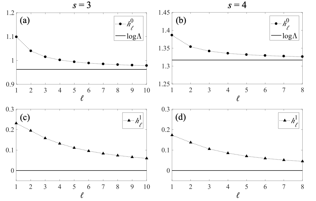
Figure 12: Geometric, $h_{\ell}^{1}$, and interior, $h_{\ell}^{0}$, parts of entropy vs. the length $\ell$ of a cat map symbol block for (a), (c) $s=3$, and (b), (d) $s=4$. The interior part of entropy $h_{\ell}^{0}$ converges to the exact value of the metric entropy, which is $\ln(3+\sqrt{5})/2$ for $s=3$ and $\ln(2+\sqrt{3})$ for $s=4$, respectively. The geometric part $h_{\ell}^{1}$ converges to $0$.

Since the Lyapunov exponents of spatiotemporal cat are known explicitly for any finite lattice, its metric entropy is known exactly, through the Pesin entropy formula [42]. On the other hand, the metric entropy can be represented through sums of symbol blocks $\mathsf{M}_{\mathcal{R}}$ measures in the limit of growing domain size $|\mathcal{R}|$. As we show below, this connection can be used to extract the asymptotics of the Jacobian $d(\mathcal{R})$ which, in turn, provides the maximum of measures for symbol blocks in a given domain $\mathcal{R}$.

C.1 Cat map entropy

Given measures ${\mu}({b})$ of blocks ${b}$ of an arbitrary finite length ${|b|}=\ell$ one can estimate observables of the dynamical system with increasing precision as $\ell$ grows. In the following we apply this to estimation of the metric entropy of the cat map.

The metric entropy of the cat map with respect to measure ${\mu}$ can be represented as the limit

$$h_{\mu}=\lim_{{\ell}\to\infty}{h}_{\ell},$$ (80)

where

$$h_{\ell}=-\frac{1}{\ell}\sum_{|{b}|=\ell}{{\mu}({b})\log{{\mu}({b})}}\,.$$

By using the decomposition (27), $h_{\ell}$ can be split as $h_{\ell}=h_{\ell}^{1}+h_{\ell}^{0}$ into “geometric” and “internal” parts:

$$h_{\ell}^{1}=-\frac{\sum_{|{b}|=\ell}{|\mathcal{P}_{{b}}|\log{|\mathcal{P}_{{b}}|}}}{\ell\sum_{|{b}|=\ell}{|\mathcal{P}_{{b}}|}},\qquad h_{\ell}^{0}=-\frac{1}{\ell}\log d_{\ell}=\frac{1}{\ell}\log U_{\ell}({s}/{2})\,.$$

The “interior” part $h_{\ell}^{0}$ converges to $\log\Lambda$ with the rate $O(1/\ell)$. Since $h_{\mu}=\log\Lambda$, the cat map metric entropy [46], the geometrical part must vanish, $\lim_{{\ell}\to\infty}h_{\ell}^{1}=0$. We illustrate this numerically for several values of $s$ in figure 12. In other words, metric entropy is determined solely by the asymptotics of the Jacobian $d_{\ell}$.

C.2 Spatiotemporal cat entropy

By the linearity of the spatiotemporal cat automorphism, every spatiotemporal cat $[{L}\!\times\!{T}]$ invariant 2-torus has the same spectrum of the Lyapunov exponents $\lambda_{k}$, $k=1,\dots,2{L}$, given by the eigenvalues (79) $\Lambda_{k}=e^{\lambda_{k}}$ of the matrix $\mathcal{B}_{\scriptscriptstyle L}$.

Accordingly, the map is fully hyperbolic iff ${2s}=a+b>4$. In this case all solutions of (79) are paired such that $\lambda_{k}^{+}=-\lambda_{k}^{-}$ and $\lambda_{k}^{+}>0$ for all $k$. The metric entropy of $\Phi_{{L}}$ for a finite ${L}$ is given by the sum of all positive exponents:

$$h(\Phi_{{L}})=\sum_{k=1}^{L}\lambda_{k}^{+}\,.$$

For the infinite lattice the corresponding spatiotemporal entropy of $\Phi$ with respect to ${\mu}$ is given by the limit $h_{\mu}(\Phi)=\lim_{L\to\infty}\frac{1}{L}{h}(\Phi_{\scriptscriptstyle L})$. Alternative, more convenient way to evaluate $h_{\mu}(\Phi)$ is to use numbers $\mathcal{N}_{{L}{T}}$ of periodic tori with spatial-temporal periods ${L},{T}$, see [29, 18]. For the linear hyperbolic automorphisms the topological and metric entropies coincide, leading to

$$h_{\mu}(\Phi) = \lim_{{L},{T}\to\infty}\frac{1}{LT}\log\mathcal{N}_{{L}{T}}$$ (81)

$$= \lim_{{L},{T}\to\infty}\frac{1}{{L}{T}}\log\mbox{det}(I-\mathcal{B}_{{L}}^{T})=\lim_{{L},{T}\to\infty}\frac{1}{{L}{T}}\log\mbox{det}(I-\mathcal{B}_{{T}}^{L})\,.$$

This yields a closed formula:

$$h_{\mu}(\Phi)=\frac{1}{\pi^{2}}\int_{0}^{\pi}\int_{0}^{\pi}\,dx\,dy\log({2s}-4+4\sin^{2}x+4\sin^{2}y)\,.$$ (82)

Recall that for the (temporal) cat map the constant $d(\mathcal{R})$ was given explicitly by (31). In the case of spatiotemporal cat we were unable to derive any explicit formula for $d(\mathcal{R})$. On the other hand, by the same argument as in the cat map case, in the large domain $\mathcal{R}$ limit the asymptotics of $d(\mathcal{R})$ is determined by the metric entropy,

$$-\lim_{|\mathcal{R}|\to\infty}\frac{1}{|\mathcal{R}|}\log d(\mathcal{R})=h_{\mu}\,,$$

where $h_{\mu}$ is the spatiotemporal metric entropy (82) of the spatiotemporal cat. Therefore, asymptotically we expect

$$d(\mathcal{R})\sim e^{-|\mathcal{R}|h_{\mu}}\,.$$ (83)

References

- [1] M. Akila et al. “Semiclassical prediction of large spectral fluctuations in interacting kicked spin chains” In Ann. Phys. 389, 2018, pp. 250–282 DOI: 10.1016/j.aop.2017.12.004
- [2] M. Akila et al. “Collectivity and periodic orbits in a chain of interacting, kicked spins” In Acta Phys. Pol. A 132, 2017, pp. 1661–1665 DOI: 10.12693/APhysPolA.132.1661
- [3] M. Akila et al. “Semiclassical identification of periodic orbits in a quantum many-body system” In Phys. Rev. Lett. 118, 2017, pp. 164101 DOI: 10.1103/physrevlett.118.164101
- [4] M. Akila, D. Waltner, B. Gutkin and T. Guhr “Particle-time duality in the kicked Ising spin chain” In J. Phys. A 49, 2016, pp. 375101 DOI: 10.1088/1751-8113/49/37/375101
- [5] V.. Arnol’d and A. Avez “Ergodic Problems of Classical Mechanics” Redwood City: Addison-Wesley, 1989
- [6] B. Bertini, P. Kos and T. Prosen “Exact spectral form factor in a minimal model of many-body quantum chaos” In Phys. Rev. Lett. 121, 2018, pp. 264101 DOI: 10.1103/PhysRevLett.121.264101
- [7] B. Bertini, P. Kos and T. Prosen “Entanglement spreading in a minimal model of maximal many-body quantum chaos” In Phys. Rev. X 9, 2019, pp. 021033 DOI: 10.1103/PhysRevX.9.021033
- [8] B. Bertini, P. Kos and T. Prosen “Exact correlation functions for dual-unitary lattice models in 1+1 dimensions” In Phys. Rev. Lett. 123, 2019, pp. 210601 DOI: 10.1103/physrevlett.123.210601
- [9] B. Bertini, P. Kos and T. Prosen “Operator entanglement in local quantum circuits i: Chaotic dual-unitary circuits” In SciPost Physics 8, 2020, pp. 067 DOI: 10.21468/SciPostPhys.8.4.067
- [10] R. Bowen “Equilibrium States and the Ergodic Theory of Anosov Diffeomorphisms” Berlin: Springer, 1975 DOI: 10.1007/bfb0081279
- [11] P. Braun et al. “Transition from quantum chaos to localization in spin chains” In Phys. Rev. E 101, 2020, pp. 052201 DOI: 10.1103/physreve.101.052201
- [12] F. Brini, S. Siboni, G. Turchetti and S. Vaienti “Decay of correlations for the automorphism of the torus ” In Nonlinearity 10, 1997, pp. 1257–1268 DOI: 10.1088/0951-7715/10/5/012
- [13] L.. Bunimovich and Ya.. Sinai “Spacetime chaos in coupled map lattices” In Nonlinearity 1, 1988, pp. 491 DOI: 10.1088/0951-7715/1/4/001
- [14] B.. Chirikov “A universal instability of many-dimensional oscillator system” In Phys. Rep. 52, 1979, pp. 263–379 DOI: 10.1016/0370-1573(79)90023-1
- [15] P.. Claeys and A. Lamacraft “Maximum velocity quantum circuits”, 2020 URL: https://arxiv.org/abs/2003.01133
- [16] S.. Creagh “Quantum zeta function for perturbed cat maps” In Chaos 5, 1995, pp. 477–493 DOI: 10.1063/1.166119
- [17] P. Cvitanović et al. “Chaos: Classical and Quantum” Copenhagen: Niels Bohr Inst., 2020 URL: http://ChaosBook.org
- [18] P. Cvitanović and H. Liang “Spatiotemporal cat: a chaotic field theory” in preparation, 2020 URL: http://ChaosBook.org/overheads/spatiotemporal/
- [19] I. Dana “General quantization of canonical maps on a two-torus” In J. Phys. A 35, 2002, pp. 3447 DOI: 10.1088/0305-4470/35/15/307
- [20] R.. Devaney “An Introduction to Chaotic Dynamical systems” Westview Press, 2008 DOI: 10.2307/3619398
- [21] F.. Dorr “The direct solution of the discrete Poisson equation on a rectangle” In SIAM Rev. 12, 1970, pp. 248–263 DOI: 10.1137/1012045
- [22] M.. Dresselhaus, G. Dresselhaus and A. Jorio “Group Theory: Application to the Physics of Condensed Matter” New York: Springer, 2007 DOI: 10.1007/978-3-540-32899-5
- [23] A.. Fetter and J.. Walecka “Theoretical Mechanics of Particles and Continua” New York: Dover, 2003
- [24] I. García-Mata and M. Saraceno “Spectral properties and classical decays in quantum open systems” In Phys. Rev. E 69, 2004, pp. 056211 DOI: 10.1103/PhysRevE.69.056211
- [25] S. Gopalakrishnan and A. Lamacraft “Unitary circuits of finite depth and infinite width from quantum channels” In Phys. Rev. B 100, 2019, pp. 064309 DOI: 10.1103/PhysRevB.100.064309
- [26] B. Gutkin et al. “Exact local correlations in kicked chains” In Phys. Rev. B 102, 2020, pp. 174307 DOI: 10.1103/physrevb.102.174307
- [27] B. Gutkin and V. Osipov “Clustering of periodic orbits and ensembles of truncated unitary matrices” In J. Stat. Phys. 153, 2013, pp. 1049–1064 DOI: 10.1007/s10955-013-0859-9
- [28] B. Gutkin and V. Osipov “Clustering of periodic orbits in chaotic systems” In Nonlinearity 26, 2013, pp. 177 DOI: 10.1088/0951-7715/26/1/177
- [29] B. Gutkin and V. Osipov “Classical foundations of many-particle quantum chaos” In Nonlinearity 29, 2016, pp. 325–356 DOI: 10.1088/0951-7715/29/2/325
- [30] J.. Hannay and M.. Berry “Quantization of linear maps on a torus – Fresnel diffraction by a periodic grating” In Physica D 1, 1980, pp. 267–290 DOI: 10.1016/0167-2789(80)90026-3
- [31] G.. Hu and R.. O’Connell “Analytical inversion of symmetric tridiagonal matrices” In J. Phys. A 29, 1996, pp. 1511 DOI: 10.1088/0305-4470/29/7/020
- [32] K. Kaneko “Transition from torus to chaos accompanied by frequency lockings with symmetry breaking: In connection with the coupled-logistic map” In Prog. Theor. Phys. 69, 1983, pp. 1427–1442 DOI: 10.1143/PTP.69.1427
- [33] K. Kaneko “Period-doubling of kink-antikink patterns, quasiperiodicity in antiferro-like structures and spatial intermittency in coupled logistic lattice: Towards a prelude of a “field theory of chaos”” In Prog. Theor. Phys. 72, 1984, pp. 480–486 DOI: 10.1143/PTP.72.480
- [34] J.. Keating “The cat maps: quantum mechanics and classical motion” In Nonlinearity 4, 1991, pp. 309–341 DOI: 10.1088/0951-7715/4/2/006
- [35] P. Kurlberg and Z. Rudnick “Hecke theory and equidistribution for the quantization of linear maps of the torus” In Duke Math. J. 103, 2000, pp. 47–77 DOI: 10.1215/S0012-7094-00-10314-6
- [36] A.. Lichtenberg and M.. Lieberman “Regular and Chaotic Dynamics” New York: Springer, 2013
- [37] P.. Martin “Discrete scattering theory: Green’s function for a square lattice” In Wave Motion 43, 2006, pp. 619–629 DOI: 10.1016/j.wavemoti.2006.05.006
- [38] B.. Mestel and I. Percival “Newton method for highly unstable orbits” In Physica D 24, 1987, pp. 172 DOI: 10.1016/0167-2789(87)90072-8
- [39] S. Müller et al. “Semiclassical foundation of universality in quantum chaos” In Phys. Rev. Lett. 93, 2004, pp. 014103 DOI: 10.1103/PhysRevLett.93.014103
- [40] I. Percival and F. Vivaldi “A linear code for the sawtooth and cat maps” In Physica D 27, 1987, pp. 373–386 DOI: 10.1016/0167-2789(87)90037-6
- [41] I. Percival and F. Vivaldi “Arithmetical properties of strongly chaotic motions” In Physica D 25, 1987, pp. 105–130 DOI: 10.1016/0167-2789(87)90096-0
- [42] Ya.. Pesin “Characteristic Lyapunov exponents and smooth ergodic theory” In Russian Math. Surveys 32, 1977, pp. 55–114 DOI: 10.1070/RM1977v032n04ABEH001639
- [43] Ya.. Pesin and Ya.. Sinai “Space-time chaos in the system of weakly interacting hyperbolic systems” In J. Geom. Phys. 5, 1988, pp. 483–492 DOI: 10.1016/0393-0440(88)90035-6
- [44] D. Ruelle “A measure associated with Axiom-A attractors” In Amer. J. Math. 98, 1976, pp. 619–654 DOI: 10.2307/2373810
- [45] M. Sieber and K. Richter “Correlations between periodic orbits and their role in spectral statistics” In Phys. Scr. 2001, 2001, pp. 128 DOI: 10.1238/Physica.Topical.090a00128
- [46] Ya.. Sinai “On the notion of entropy of a dynamical system” In Selecta I 124 New York: Springer, 1959, pp. 768–771
- [47] J. Slipantschuk, O.. Bandtlow and W. Just “Complete spectral data for analytic Anosov maps of the torus” In Nonlinearity 30, 2017, pp. 2667 DOI: 10.1088/1361-6544/aa700f
- [48] R. Sturman, J.. Ottino and S. Wiggins “The Mathematical Foundations of Mixing” Cambridge Univ. Press, 2006
- [49] R.. Vallejos and M. Saraceno “The construction of a quantum Markov partition” In J. Phys. A 32, 1999, pp. 7273 DOI: 10.1088/0305-4470/32/42/304
- [50] Wolfram Research, Inc. “Mathematica 11”, 2017 URL: https://www.wolfram.com/mathematica/