Risk-Aware MMSE Estimation

Abstract

Despite the simplicity and intuitive interpretation of Minimum Mean Squared Error (MMSE) estimators, their effectiveness in certain scenarios is questionable. Indeed, minimizing squared errors on average does not provide any form of stability, as the volatility of the estimation error is left unconstrained. When this volatility is statistically significant, the difference between the average and realized performance of the MMSE estimator can be drastically different. To address this issue, we introduce a new risk-aware MMSE formulation which trades between mean performance and risk by explicitly constraining the expected predictive variance of the involved squared error. We show that, under mild moment boundedness conditions, the corresponding risk-aware optimal solution can be evaluated explicitly, and has the form of an appropriately biased nonlinear MMSE estimator. We further illustrate the effectiveness of our approach via several numerical examples, which also showcase the advantages of risk-aware MMSE estimation against risk-neutral MMSE estimation, especially in models involving skewed, heavy-tailed distributions.

Keywords. MMSE Estimation, Constrained Bayesian Estimation, Risk-Aware Optimization, Risk Measures.

1 Introduction

Critical applications require that stochastic decisions be made not only on the basis of minimizing average losses, but also safeguarding against less probable, though possibly catastrophic, events. Examples appear naturally in many areas, including wireless industrial control [1], energy [2, 3], finance [4, 5, 6], robotics [7, 8], LIDAR [9], and networking [10]. In such cases, the ultimate goal is to obtain risk-aware decision policies that hedge against statistically significant extreme losses, even at the cost of slightly sacrificing performance under nominal operating conditions.

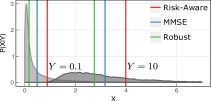
Figure 1: Comparison between risk-neutral and risk-aware estimates.

To illustrate this effect, consider the problem of estimating a random state $X$ from observations corrupted by state-dependent noise, namely $Y|X\sim{\cal N}(X,9X^{2})$ (see Section 5). In such a setting, either small or large values of $Y$ provide highly ambiguous evidence, since, in both cases, they can come from either small or large values of $X$. This is corroborated by Fig. 1, which displays the posterior distribution ${\cal P}_{X|Y}$ for two values of $Y$. While the MMSE estimator may incur severe losses, the risk-aware estimator we develop in this work – shown as red vertical lines in Fig. 1 – hedges against observation ambiguity, therefore avoiding extreme prediction errors. Such behavior is achieved by biasing estimates towards the tail of the posterior ${\cal P}_{X|Y}$, by the right amount, for each realization of $Y$. Although the risk-aware estimator may incur larger losses on average, it performs statistically more consistently across realizations of $Y$ (also see risk curve in Fig. 2, Section 5). It is also worth contrasting risk-awareness with statistical robustness, whose goal is to protect against deviations from a nominal model. Robust estimators – green vertical lines in Fig. 1 – promote insensitivity to tail events, which they designate as statistically insignificant. On the other hand, estimators resulting from risk-aware formulations treat these events as statistically significant, though relatively infrequent (see Table 1).

Over the last three decades, risk-aware optimization has grown increasingly popular and has been studied in the contexts of both decision making and learning [11, 12, 13, 14, 15, 16, 17, 18]. In risk-aware optimization, expectations are replaced by more general functionals, called risk measures [19], whose purpose is to quantify the statistical volatility of random losses, as well as mean performance. Popular examples include mean-variance functionals [4, 19], mean-semideviations [15], and Conditional Value-at-Risk (CVaR) [20].

In Bayesian estimation, risk awareness is typically achieved by replacing the classical quadratic cost with its exponentiation [21, 22, 23, 24, 25]. However, although sometimes effective, this approach is not without limitations. First, the need for finiteness of the moment generating function of the quadratic cost excludes heavy-tailed distributions, which are precisely those that incur high risk. Second, the exponential approach does not provide an interpretable way to control the trade-off between mean performance and risk, making it hard to use in settings where explicit risk levels must be met. Third, it does not result in a simple, general solution as in classical MMSE estimation, challenging its practical applicability. Finally, it does not effectively quantify observation-induced risk, inherent in problems where measurements provide ambiguous evidence.

Uncertainty	Frequent	Infrequent
Significant	Model	Risk
Insignificant	Noise	Outliers

Table 1: Classification of statistical uncertainty.

In this work, we pose risk-aware functional Bayesian estimation as a constrained MMSE problem, where squared errors are minimized on average, subject to a bound on their expected conditional variance. We show that, under mild conditions, this formulation results in a convex variational problem that admits a closed-form solution. The resulting optimal risk-aware nonlinear MMSE estimator is applicable to a wide variety of generative models, including highly skewed and/or heavy-tailed distributions. The effectiveness of our approach is confirmed via numerical examples, also demonstrating its advantages against risk-neutral MMSE estimation.

2 Problem Formulation

Let $(\Omega,\mathscr{F},{\cal P})$ be a probability space, and consider an arbitrary pair of random elements $\boldsymbol{X}:\Omega\rightarrow\mathbb{R}^{M}$ and $\boldsymbol{Y}:\Omega\rightarrow\mathbb{R}^{N}$ on $(\Omega,\mathscr{F})$. We are interested in the problem of estimating $\boldsymbol{X}$ from a single realization of $\boldsymbol{Y}$ in a Bayesian setting, namely by assuming knowledge of the joint probability distribution ${\cal P}_{(\boldsymbol{X},\boldsymbol{Y})}$. We may conveniently think of $\boldsymbol{Y}$ as available observations, on the basis of which we would like to make predictions about the hidden state $\boldsymbol{X}$. Undoubtedly, this general problem is fundamental in many areas, including statistics, signal processing, machine learning, and control, and with numerous interesting applications.

Of course, an established approach to the prediction problem considered is to choose an estimator $\widehat{\boldsymbol{X}}:\Omega\rightarrow\mathbb{R}^{M}$ as a solution to the stochastic variational MMSE program

$$\begin{array}[]{rl}\underset{\widehat{\boldsymbol{X}}:\Omega\rightarrow\mathbb{R}^{M}}{\mathrm{minimize}}&\mathbb{E}\{\|\boldsymbol{X}-\widehat{\boldsymbol{X}}\|_{2}^{2}\}\\ \mathrm{subject\,to}&\widehat{\boldsymbol{X}}\text{ is }\mathscr{Y}\text{-measurable}\end{array},$$ (1)

where $\mathscr{Y}\equiv\sigma\{\boldsymbol{Y}\}$ denotes the sub-$\sigma$-algebra of $\mathscr{F}$ generated by $\boldsymbol{Y}$. Problem (1) is well-understood under rather general conditions. In fact, if we merely assume that $\boldsymbol{X}\in{\cal L}_{1}(\Omega,\mathscr{Y},{\cal P};\mathbb{R}^{M})\equiv{\cal L}_{1|\mathscr{Y}}^{M}$, an optimal solution to (1) is given by any conditional expectation of $\boldsymbol{X}$ relative to $\boldsymbol{Y}$, i.e., $\widehat{\boldsymbol{X}}^{*}(\boldsymbol{Y})\equiv\mathbb{E}\{\boldsymbol{X}|\boldsymbol{Y}\}$.

However, despite the simplicity of MMSE estimation, as well as its intuitive geometric interpretation in Hilbert space whenever $\boldsymbol{X}\in{\cal L}_{2|\mathscr{Y}}^{M}$, its effectiveness is often questionable. Indeed, minimizing the squared error $\|\boldsymbol{X}-\widehat{\boldsymbol{X}}\|_{2}^{2}$ in expectation does not provide stability or robustness, in the sense that statistically significant variability of the resulting optimal prediction error is uncontrolled. In other words, the MMSE problem (1) is risk-neutral. This has important consequences from a practical perspective, since the error realization $\|\boldsymbol{X}-\widehat{\boldsymbol{X}}^{*}(\boldsymbol{Y})\|_{2}^{2}$ experienced in practice may be far from the expected value $\mathbb{E}\{\|\boldsymbol{X}-\widehat{\boldsymbol{X}}^{*}(\boldsymbol{Y})\|_{2}^{2}\}$, or even the predictive statistic $\mathbb{E}\{\|\boldsymbol{X}-\widehat{\boldsymbol{X}}^{*}(\boldsymbol{Y})\|_{2}^{2}|\boldsymbol{Y}\}$. It is then clear that achieving small error variability is at least as desirable as achieving minimal errors on average.

Motivated by the previous discussion, we consider a nontrivial variation of the risk-neutral MMSE problem (1), striking a balance between mean performance and risk. Specifically, we introduce and study the constrained stochastic variational problem

$$\begin{array}[]{rl}\underset{\widehat{\boldsymbol{X}}:\Omega\rightarrow\mathbb{R}^{M}}{\mathrm{minimize}}&\mathbb{E}\{\|\boldsymbol{X}-\widehat{\boldsymbol{X}}\|_{2}^{2}\}\\ \mathrm{subject\,to}&\mathbb{E}\{\mathbb{V}_{\boldsymbol{Y}}\{\|\boldsymbol{X}-\widehat{\boldsymbol{X}}\|_{2}^{2}\}\}\leq\varepsilon\\ &\widehat{\boldsymbol{X}}\text{ is }\mathscr{Y}\text{-measurable}\end{array},$$ (2)

where

$$\mathbb{V}_{\boldsymbol{Y}}\{\|\boldsymbol{X}-\widehat{\boldsymbol{X}}\|_{2}^{2}\}\triangleq\mathbb{E}\big{\{}\big{(}\|\boldsymbol{X}-\widehat{\boldsymbol{X}}\|_{2}^{2}-\mathbb{E}\{\|\boldsymbol{X}-\widehat{\boldsymbol{X}}\|_{2}^{2}|\boldsymbol{Y}\}\big{)}^{2}|\boldsymbol{Y}\big{\}}$$ (3)

is the predictive variance of $\|\boldsymbol{X}-\widehat{\boldsymbol{X}}\|_{2}^{2}$ relative to $\boldsymbol{Y}$, and $\varepsilon>0$ is a fixed risk tolerance. In words, problem (2) constrains the expected predictive variance of the quadratic cost $\|\boldsymbol{X}-\widehat{\boldsymbol{X}}\|_{2}^{2}$, known in the statistics literature as the unexplained component of its variance; the latter is due to the law of total variance. In other words, the constraint quantifies the uncertainty of MMSE-optimally predicting the quadratic cost achieved by choosing an estimator $\widehat{\boldsymbol{X}}(\boldsymbol{Y})$, on the basis of the observations $\boldsymbol{Y}$. Of course, $\mathbb{E}\{\mathbb{V}_{\boldsymbol{Y}}\{\|\boldsymbol{X}-\widehat{\boldsymbol{X}}\|_{2}^{2}\}\}$ is a measure of risk. Therefore, we suggestively refer to the task fulfilled by problem (2) as risk-aware MMSE estimation.

Problem (2) confines the search for an optimal MMSE estimator within the family of estimators exhibiting risk (in the sense described above) within tolerance $\varepsilon$; thus, problem (2) is well-motivated. Naturally, an optimal solution to the risk-aware problem (2) in general achieves larger MSE as compared to the risk-neutral problem (1). However, the statistical variability of the squared errors achieved by the former will be explicitly controlled, according to the tunable tolerance $\varepsilon$, resulting in more stable statistical prediction.

3 Convex Variational QCQP Reformulation

As it turns out, in such a general form, the risk-aware MMSE problem (2) is rather challenging to study, let alone solve. Therefore, in the following, we will consider a slightly more constrained version of (2), by enforcing square integrability on the decision $\widehat{\boldsymbol{X}}$, namely,

$$\begin{array}[]{rl}\underset{\widehat{\boldsymbol{X}}:\Omega\rightarrow\mathbb{R}^{M}}{\mathrm{minimize}}&\mathbb{E}\{\|\boldsymbol{X}-\widehat{\boldsymbol{X}}\|_{2}^{2}\}\\ \mathrm{subject\,to}&\mathbb{E}\{\mathbb{V}_{\boldsymbol{Y}}\{\|\boldsymbol{X}-\widehat{\boldsymbol{X}}\|_{2}^{2}\}\}\leq\varepsilon\\ &\widehat{\boldsymbol{X}}\in{\cal L}_{2|\mathscr{Y}}^{M}\end{array}.$$ (4)

Of course, the additional ${\cal L}_{2}$ constraint in problem (4) may not be in favor of generality, per se, but it is harmless for almost every practical consideration. Further, in the following we make use of the following regularity condition on the statistical behavior of $(\boldsymbol{X},\boldsymbol{Y})$.

Assumption 1.

It is true that $\mathbb{E}\big{\{}\|\boldsymbol{X}\|_{2}^{3}|\boldsymbol{Y}\big{\}}\in{\cal L}_{2|\mathscr{Y}}^{1}$.

In words, Assumption 1 simply says that the third-order moment filter $\mathbb{E}\big{\{}\|\boldsymbol{X}\|_{2}^{3}|\boldsymbol{Y}\big{\}}$ is of finite energy. Using Assumption 1, problem (4) may be conveniently reformulated, as the next result suggests.

Lemma 1.

(QCQP Reformulation of Problem (4)) Suppose that Assumption 1 is in effect, and define the posterior covariance

$$\boldsymbol{\Sigma}_{\boldsymbol{X}|\boldsymbol{Y}}\triangleq\mathbb{E}\big{\{}(\boldsymbol{X}-\mathbb{E}\{\boldsymbol{X}|\boldsymbol{Y}\})(\boldsymbol{X}-\mathbb{E}\{\boldsymbol{X}|\boldsymbol{Y}\})^{\boldsymbol{T}}|\boldsymbol{Y}\big{\}}\succeq{\bf 0}.$$ (5)

Then, problem (4) is well-defined and equivalent to the convex variational Quadratically Constrained Quadratic Program (QCQP)

$$\begin{array}[]{rl}\underset{\widehat{\boldsymbol{X}}:\Omega\rightarrow\mathbb{R}^{M}}{\mathrm{minimize}}&\dfrac{1}{2}\mathbb{E}\big{\{}\|\widehat{\boldsymbol{X}}\|_{2}^{2}-2(\mathbb{E}\big{\{}\boldsymbol{X}|\boldsymbol{Y}\big{\}})^{\boldsymbol{T}}\widehat{\boldsymbol{X}}+\mathbb{E}\big{\{}\|\boldsymbol{X}\|_{2}^{2}|\boldsymbol{Y}\big{\}}\big{\}}\\ \mathrm{subject\,to}&\mathbb{E}\big{\{}\widehat{\boldsymbol{X}}^{\boldsymbol{T}}\boldsymbol{\Sigma}_{\boldsymbol{X}|\boldsymbol{Y}}\widehat{\boldsymbol{X}}-\big{(}\mathbb{E}\big{\{}\|\boldsymbol{X}\|_{2}^{2}\boldsymbol{X}|\boldsymbol{Y}\big{\}}\\ &\quad-\mathbb{E}\big{\{}\|\boldsymbol{X}\|_{2}^{2}|\boldsymbol{Y}\big{\}}\mathbb{E}\{\boldsymbol{X}|\boldsymbol{Y}\}\big{)}^{\boldsymbol{T}}\widehat{\boldsymbol{X}}\big{\}}\\ &\quad\quad\leq\dfrac{\varepsilon-\mathbb{E}\big{\{}\mathbb{V}_{\boldsymbol{Y}}\{\|\boldsymbol{X}\|_{2}^{2}\}\big{\}}}{4}\\ &\widehat{\boldsymbol{X}}\in{\cal L}_{2|\mathscr{Y}}^{M}\end{array},$$ (6)

where all expectations and involved operations are well-defined.

Proof of Lemma 1.

We start with the objective of problem (4), for which it is obviously true that

$$\mathbb{E}\{\|\boldsymbol{X}-\widehat{\boldsymbol{X}}\|_{2}^{2}\}\equiv\mathbb{E}\big{\{}\mathbb{E}\big{\{}\|\boldsymbol{X}\|_{2}^{2}-2\boldsymbol{X}^{\boldsymbol{T}}\widehat{\boldsymbol{X}}+\|\widehat{\boldsymbol{X}}\|_{2}^{2}|\boldsymbol{Y}\big{\}}\big{\}},$$ (7)

since the expectation of $\|\boldsymbol{X}-\widehat{\boldsymbol{X}}\|_{2}^{2}$ always exists. Additionally, by invoking Cauchy-Schwarz twice, we observe that

$$\mathbb{E}\big{\{}|\boldsymbol{X}^{\boldsymbol{T}}\widehat{\boldsymbol{X}}|\big{\}} \leq\mathbb{E}\big{\{}\|\boldsymbol{X}\|_{2}\|\widehat{\boldsymbol{X}}\|_{2}\big{\}}$$

$$\equiv\mathbb{E}\big{\{}\mathbb{E}\big{\{}\|\boldsymbol{X}\|_{2}|\boldsymbol{Y}\big{\}}\|\widehat{\boldsymbol{X}}\|_{2}\big{\}}$$

$$\leq\big{\|}\mathbb{E}\big{\{}\|\boldsymbol{X}\|_{2}|\boldsymbol{Y}\big{\}}\big{\|}_{{\cal L}_{2}}\big{\|}\|\widehat{\boldsymbol{X}}\|_{2}\big{\|}_{{\cal L}_{2}},$$ (8)

where $\big{\|}\|\widehat{\boldsymbol{X}}\|_{2}\big{\|}_{{\cal L}_{2}}<\infty\iff\widehat{\boldsymbol{X}}\in{\cal L}_{2|\mathscr{Y}}^{M}$ by assumption, and Jensen implies that

$$\big{\|}\mathbb{E}\big{\{}\|\boldsymbol{X}\|_{2}|\boldsymbol{Y}\big{\}}\big{\|}_{{\cal L}_{2}} \leq\big{\|}\mathbb{E}\big{\{}\|\boldsymbol{X}\|_{2}|\boldsymbol{Y}\big{\}}\big{\|}_{{\cal L}_{3}}$$

$$\leq\big{(}\mathbb{E}\big{\{}\big{(}\mathbb{E}\big{\{}\|\boldsymbol{X}\|_{2}^{3}|\boldsymbol{Y}\big{\}}\big{)}^{2\cdot 1/2}\big{\}}\big{)}^{1/3}$$

$$\leq\big{(}\mathbb{E}\big{\{}\big{(}\mathbb{E}\big{\{}\|\boldsymbol{X}\|_{2}^{3}|\boldsymbol{Y}\big{\}}\big{)}^{2}\big{\}}\big{)}^{1/(2\cdot 3)}$$

$$\leq\big{\|}\mathbb{E}\big{\{}\|\boldsymbol{X}\|_{2}^{3}|\boldsymbol{Y}\big{\}}\big{\|}_{{\cal L}_{2}}^{1/3}<\infty,$$ (9)

as well. Then $\mathbb{E}\big{\{}\boldsymbol{X}^{\boldsymbol{T}}\widehat{\boldsymbol{X}}\big{\}}$ is finite, and it follows that

$$\mathbb{E}\{\|\boldsymbol{X}-\widehat{\boldsymbol{X}}\|_{2}^{2}\}\equiv\mathbb{E}\big{\{}\|\widehat{\boldsymbol{X}}\|_{2}^{2}-2(\mathbb{E}\big{\{}\boldsymbol{X}|\boldsymbol{Y}\big{\}})^{\boldsymbol{T}}\widehat{\boldsymbol{X}}+\mathbb{E}\big{\{}\|\boldsymbol{X}\|_{2}^{2}|\boldsymbol{Y}\big{\}}\big{\}},$$ (10)

as in the objective of (6).

The constraint of (4) may be equivalently reexpressed in a similar fashion, although the procedure is slightly more involved. Specifically, by definition of $\mathbb{V}_{\boldsymbol{Y}}\{\|\boldsymbol{X}-\widehat{\boldsymbol{X}}\|_{2}^{2}\}$, we may initially expand as

$$\big{(}\|\boldsymbol{X}-\widehat{\boldsymbol{X}}\|_{2}^{2}-\mathbb{E}\{\|\boldsymbol{X}-\widehat{\boldsymbol{X}}\|_{2}^{2}|\boldsymbol{Y}\}\big{)}^{2}$$

$$\equiv(\|\boldsymbol{X}\|_{2}^{2}-\mathbb{E}\{\|\boldsymbol{X}\|_{2}^{2}|\boldsymbol{Y}\})^{2}+4\widehat{\boldsymbol{X}}^{\boldsymbol{T}}(\boldsymbol{X}-\mathbb{E}\{\boldsymbol{X}|\boldsymbol{Y}\})(\boldsymbol{X}-\mathbb{E}\{\boldsymbol{X}|\boldsymbol{Y}\})^{\boldsymbol{T}}\widehat{\boldsymbol{X}}$$

$$\quad-4\|\boldsymbol{X}\|_{2}^{2}\boldsymbol{X}^{\boldsymbol{T}}\widehat{\boldsymbol{X}}+4\|\boldsymbol{X}\|_{2}^{2}(\mathbb{E}\{\boldsymbol{X}|\boldsymbol{Y}\})^{\boldsymbol{T}}\widehat{\boldsymbol{X}}$$

$$\quad\quad+4\mathbb{E}\{\|\boldsymbol{X}\|_{2}^{2}|\boldsymbol{Y}\}\boldsymbol{X}^{\boldsymbol{T}}\widehat{\boldsymbol{X}}-4\mathbb{E}\{\|\boldsymbol{X}\|_{2}^{2}|\boldsymbol{Y}\}(\mathbb{E}\{\boldsymbol{X}|\boldsymbol{Y}\})^{\boldsymbol{T}}\widehat{\boldsymbol{X}},$$ (11)

where the first two terms of the right-hand side of (11) are nonnegative. Consequently, it suffices to concentrate on the respective last four dot product terms.

Using the same argument as in (8), in order to show that all these four terms have finite expectations, it suffices to ensure that

$$\big{\|}\mathbb{E}\{\|\|\boldsymbol{X}\|_{2}^{2}\boldsymbol{X}\|_{2}|\boldsymbol{Y}\}\big{\|}_{{\cal L}_{2}}\equiv\big{\|}\mathbb{E}\{\|\boldsymbol{X}\|_{2}^{3}|\boldsymbol{Y}\}\big{\|}_{{\cal L}_{2}}<\infty,$$ (12)

which is of course automatically true by Assumption 1, but also that

$$\big{\|}\mathbb{E}\{\|\|\boldsymbol{X}\|_{2}^{2}\mathbb{E}\{\boldsymbol{X}|\boldsymbol{Y}\}\|_{2}|\boldsymbol{Y}\}\big{\|}_{{\cal L}_{2}} \equiv\big{\|}\mathbb{E}\{\|\boldsymbol{X}\|_{2}^{2}\|\mathbb{E}\{\boldsymbol{X}|\boldsymbol{Y}\}\|_{2}|\boldsymbol{Y}\}\big{\|}_{{\cal L}_{2}}$$

$$\equiv\big{\|}\|\mathbb{E}\{\boldsymbol{X}|\boldsymbol{Y}\}\|_{2}\mathbb{E}\{\|\boldsymbol{X}\|_{2}^{2}|\boldsymbol{Y}\}\big{\|}_{{\cal L}_{2}}$$

$$<\infty,$$ (13)

$$\big{\|}\mathbb{E}\{\|\mathbb{E}\{\|\boldsymbol{X}\|_{2}^{2}|\boldsymbol{Y}\}\boldsymbol{X}\|_{2}|\boldsymbol{Y}\}\big{\|}_{{\cal L}_{2}} \equiv\big{\|}\mathbb{E}\{\|\boldsymbol{X}\|_{2}|\boldsymbol{Y}\}\mathbb{E}\{\|\boldsymbol{X}\|_{2}^{2}|\boldsymbol{Y}\}\big{\|}_{{\cal L}_{2}}$$

$$<\infty\quad\text{and}$$ (14)

$$\big{\|}\mathbb{E}\big{\{}\|\mathbb{E}\{\|\boldsymbol{X}\|_{2}^{2}|\boldsymbol{Y}\big{\}}\mathbb{E}\{\boldsymbol{X}|\boldsymbol{Y}\}\|_{2}|\boldsymbol{Y}\}\big{\|}_{{\cal L}_{2}} \equiv\big{\|}\|\mathbb{E}\{\boldsymbol{X}|\boldsymbol{Y}\}\|_{2}\mathbb{E}\{\|\boldsymbol{X}\|_{2}^{2}|\boldsymbol{Y}\}\big{\|}_{{\cal L}_{2}}$$ (15)

$$<\infty.$$ (16)

Observe, though, that all three latter quantities are upper bounded by the quantity $\big{\|}\mathbb{E}\{\|\boldsymbol{X}\|_{2}|\boldsymbol{Y}\}\mathbb{E}\{\|\boldsymbol{X}\|_{2}^{2}|\boldsymbol{Y}\}\big{\|}_{{\cal L}_{2}}$, for which we may write (by Jensen)

$$\big{\|}\mathbb{E}\{\|\boldsymbol{X}\|_{2}|\boldsymbol{Y}\}\mathbb{E}\{\|\boldsymbol{X}\|_{2}^{2}|\boldsymbol{Y}\}\big{\|}_{{\cal L}_{2}}^{2} \equiv\mathbb{E}\big{\{}(\mathbb{E}\{\|\boldsymbol{X}\|_{2}|\boldsymbol{Y}\})^{2}(\mathbb{E}\{\|\boldsymbol{X}\|_{2}^{2}|\boldsymbol{Y}\})^{2}\big{\}}$$

$$\leq\mathbb{E}\big{\{}\mathbb{E}\{\|\boldsymbol{X}\|_{2}^{2}|\boldsymbol{Y}\}(\mathbb{E}\{\|\boldsymbol{X}\|_{2}^{2}|\boldsymbol{Y}\})^{2}\big{\}}$$

$$\equiv\mathbb{E}\big{\{}(\mathbb{E}\{\|\boldsymbol{X}\|_{2}^{2}|\boldsymbol{Y}\})^{3}\big{\}}$$

$$\equiv\mathbb{E}\big{\{}(\mathbb{E}\{\|\boldsymbol{X}\|_{2}^{2}|\boldsymbol{Y}\})^{2\cdot 3/2}\big{\}}$$

$$\leq\mathbb{E}\big{\{}(\mathbb{E}\{\|\boldsymbol{X}\|_{2}^{3}|\boldsymbol{Y}\})^{2}\big{\}}<\infty,$$ (17)

where the last line follows again by Assumption 1.

Given the discussion above, we may now take conditional expectations on (11), to obtain the expression (note that all operations involving conditional expectations are technically allowed under our assumptions)

$$\mathbb{V}_{\boldsymbol{Y}}\{\|\boldsymbol{X}-\widehat{\boldsymbol{X}}\|_{2}^{2}\}$$

$$\equiv\mathbb{E}\big{\{}\big{(}\|\boldsymbol{X}-\widehat{\boldsymbol{X}}\|_{2}^{2}-\mathbb{E}\{\|\boldsymbol{X}-\widehat{\boldsymbol{X}}\|_{2}^{2}|\boldsymbol{Y}\}\big{)}^{2}|\boldsymbol{Y}\big{\}}$$

$$\equiv\mathbb{V}_{\boldsymbol{Y}}\{\|\boldsymbol{X}\|_{2}^{2}\}+4\widehat{\boldsymbol{X}}^{\boldsymbol{T}}\boldsymbol{\Sigma}_{\boldsymbol{X}|\boldsymbol{Y}}\widehat{\boldsymbol{X}}$$

$$\quad-4\big{(}\mathbb{E}\{\|\boldsymbol{X}\|_{2}^{2}\boldsymbol{X}|\boldsymbol{Y}\}-\mathbb{E}\{\|\boldsymbol{X}\|_{2}^{2}|\boldsymbol{Y}\}\mathbb{E}\{\boldsymbol{X}|\boldsymbol{Y}\}\big{)}^{\boldsymbol{T}}\widehat{\boldsymbol{X}}.$$ (18)

Taking expectations on both sides of (18) and rearranging terms gives the desired expression for the constraint of the QCQP (6). ∎

Lemma 1 is very useful, because it shows the equivalence of problem (4) to the convex QCQP (6), which is well-defined and favorably structured. In particular, this reformulation will allow us to effectively study problem (4) by looking at its variational Lagrangian dual. Actually, as we discuss next, working in the dual domain will allow us to solve problem (4) in closed-form. Of course, such a closed form is important, not only because it provides an analytical, textbook-level solution to a functional risk-aware problem, which happens rather infrequently in such settings, but also because, as we will see, the solution itself provides intuition, highlights connections and enables comparison of problem (4) with its risk-neutral counterpart (1).

4 Risk-Aware MMSE Estimators

In our development, we exploit a variational version of Slater’s condition, which is one the most widely used constraint qualifications in both deterministic and stochastic optimization.

Assumption 2.

Given $\varepsilon>0$, problem (4) satisfies Slater’s condition, i.e., there exists $\widehat{\boldsymbol{X}}_{\dagger}\in{\cal L}_{2|\mathscr{Y}}^{M}$, such that $\mathbb{E}\{\|\boldsymbol{X}-\widehat{\boldsymbol{X}}_{\dagger}\|_{2}^{2}\}<\infty$ and $\mathbb{E}\{\mathbb{V}_{\boldsymbol{Y}}\{\|\boldsymbol{X}-\widehat{\boldsymbol{X}}_{\dagger}\|_{2}^{2}\}\}<\varepsilon$.

Under both Assumptions 1 and 2, it follows that the QCQP (6) satisfies Slater’s condition, as well. Then, it must be the case that $\mathbb{E}\{\mathbb{V}_{\boldsymbol{Y}}\{\|\boldsymbol{X}\|_{2}^{2}\}\}<\infty$; if not, Assumption 2 is impossible to hold. Further, problem (6) must be feasible, with convex effective domain

$${\cal F}_{2|\mathscr{Y}}^{M}\triangleq\big{\{}\widehat{\boldsymbol{X}}\in{\cal L}_{2|\mathscr{Y}}^{M}\big{|}\mathbb{E}\big{\{}\widehat{\boldsymbol{X}}^{\boldsymbol{T}}\boldsymbol{\Sigma}_{\boldsymbol{X}|\boldsymbol{Y}}\widehat{\boldsymbol{X}}\big{\}}<\infty\big{\}}.$$ (19)

Next, if Assumption 1 holds, define the variational Lagrangian of the primal problem (6) $\mathpzc{L}:{\cal L}_{2|\mathscr{Y}}^{M}$ $\times\mathbb{R}_{+}\rightarrow(-\infty,\infty]$ as

$$\mathpzc{L}\big{(}\widehat{\boldsymbol{X}},\mu\big{)} \triangleq\dfrac{1}{2}\mathbb{E}\big{\{}\|\widehat{\boldsymbol{X}}\|_{2}^{2}-2(\mathbb{E}\big{\{}\boldsymbol{X}|\boldsymbol{Y}\big{\}})^{\boldsymbol{T}}\widehat{\boldsymbol{X}}+\mathbb{E}\big{\{}\|\boldsymbol{X}\|_{2}^{2}|\boldsymbol{Y}\big{\}}\big{\}}$$

$$\quad+\mu\mathbb{E}\big{\{}\widehat{\boldsymbol{X}}^{\boldsymbol{T}}\boldsymbol{\Sigma}_{\boldsymbol{X}|\boldsymbol{Y}}\widehat{\boldsymbol{X}}-\big{(}\mathbb{E}\big{\{}\|\boldsymbol{X}\|_{2}^{2}\boldsymbol{X}|\boldsymbol{Y}\big{\}}$$

$$\quad\quad-\mathbb{E}\big{\{}\|\boldsymbol{X}\|_{2}^{2}|\boldsymbol{Y}\big{\}}\mathbb{E}\{\boldsymbol{X}|\boldsymbol{Y}\}\big{)}^{\boldsymbol{T}}\widehat{\boldsymbol{X}}\big{\}}$$

$$\quad\quad\quad-\mu\dfrac{\varepsilon-\mathbb{E}\big{\{}\mathbb{V}_{\boldsymbol{Y}}\{\|\boldsymbol{X}\|_{2}^{2}\}\big{\}}}{4},$$ (20)

where $\mu\in\mathbb{R}_{+}$ is a multiplier associated with the constraint of (6). The dual function $\mathpzc{D}:\mathbb{R}_{+}\rightarrow(-\infty,\infty]$ is accordingly defined as

$$\mathpzc{D}(\mu)\triangleq\inf_{\widehat{\boldsymbol{X}}\in{\cal F}_{2|\mathscr{Y}}^{M}}\mathpzc{L}\big{(}\widehat{\boldsymbol{X}},\mu\big{)}.$$ (21)

If $\mathpzc{P}^{*}\in[0,\infty]$ denotes the optimal value of problem (6), it is true that $\mathpzc{D}\leq\mathpzc{P}^{*}$ on $\mathbb{R}_{+}$. Then, the optimal value of the always concave, dual problem

$$\begin{array}[]{rl}\mathrm{maximize}&\mathpzc{D}(\mu)\\ \mathrm{subject\,to}&\mu\geq 0\end{array},$$ (22)

defined as $\mathpzc{D}^{*}\triangleq\sup_{\mu\geq 0}\mathpzc{D}(\mu)\in(-\infty,\infty]$, is the tightest under-estimate of $\mathpzc{P}^{*}$, when knowing only $\mathpzc{D}$.

Exploiting Assumptions 1 and 2, we may now formulate the following fundamental theorem, which establishes that the convex variational problem (6) exhibits zero duality gap. This essentially follows as an application of standard results in variational Lagrangian duality; see, for instance, ([26], Section 8.3, Theorem 1). The proof is therefore straightforward, and omitted.

Theorem 1.

(QCQP (6): Zero Duality Gap) Suppose that Assumptions 1 and 2 are in effect. Then, strong duality holds for problem (6), that is, $0\leq\mathpzc{D}^{*}\equiv\mathpzc{P}^{*}<\infty$. Additionally, the set of dual optimal solutions, $\arg\max_{\mu\geq 0}\mathpzc{D}(\mu)$, is nonempty. Further, if $\widehat{\boldsymbol{X}}_{*}$ is primal optimal for (6), it follows that $\widehat{\boldsymbol{X}}_{*}\equiv\widehat{\boldsymbol{X}}_{*}(\mu_{*})\in\arg\min_{\widehat{\boldsymbol{X}}\in{\cal F}_{2|\mathscr{Y}}^{M}}\mathpzc{L}\big{(}\widehat{\boldsymbol{X}},\mu_{*}\big{)}$, where $0\leq\mu_{*}\in\arg\max_{\mu\geq 0}\mathpzc{D}(\mu)$.

Leveraging Theorem 1, it is possible to show that, under Assumptions 1 and 2, the QCQP (6) and, therefore, the original ${\cal L}_{2}$ risk-aware MMSE problem (4), admit a common closed form solution. In this respect, we have the next theorem, which constitutes the main result of this paper.

Theorem 2.

(QCQP (6): Closed-Form Solution) Suppose that Assumptions 1 and 2 are in effect. Then, an optimal solution to problem (6) may be expressed as (with slight abuse of notation)

$$\boxed{\widehat{\boldsymbol{X}}_{*}(\mu_{*})\equiv\dfrac{\mathbb{E}\big{\{}\boldsymbol{X}|\boldsymbol{Y}\big{\}}+\mu_{*}\big{(}\mathbb{E}\big{\{}\|\boldsymbol{X}\|_{2}^{2}\boldsymbol{X}|\boldsymbol{Y}\big{\}}-\mathbb{E}\big{\{}\|\boldsymbol{X}\|_{2}^{2}|\boldsymbol{Y}\big{\}}\mathbb{E}\{\boldsymbol{X}|\boldsymbol{Y}\}\big{)}}{\boldsymbol{I}+2\mu_{*}\boldsymbol{\Sigma}_{\boldsymbol{X}|\boldsymbol{Y}}},}$$ (23)

with $\widehat{\boldsymbol{X}}_{*}(\mu_{*})\in\arg\min_{\widehat{\boldsymbol{X}}\in{\cal F}_{2|\mathscr{Y}}^{M}}\mathpzc{L}\big{(}\widehat{\boldsymbol{X}},\mu_{*}\big{)}$, and where $\mu_{*}\equiv\mu_{*}(\varepsilon)\in\mathbb{R}_{+}$ is an optimal solution to the concave dual problem

$$\sup_{\mu\geq 0}\mathpzc{D}(\mu) \equiv\sup_{\mu\geq 0}\inf_{\widehat{\boldsymbol{X}}\in{\cal F}_{2|\mathscr{Y}}^{M}}\mathpzc{L}\big{(}\widehat{\boldsymbol{X}},\mu\big{)}$$

$$\equiv\dfrac{1}{2}\mathbb{E}\big{\{}\|\boldsymbol{X}\|_{2}^{2}\big{\}}+\dfrac{1}{4}\sup_{\mu\geq 0}\Big{\{}\mu\mathbb{E}\big{\{}\mathbb{V}_{\boldsymbol{Y}}\{\|\boldsymbol{X}\|_{2}^{2}\}\big{\}}$$

$$\quad-2\mathbb{E}\big{\{}\widehat{\boldsymbol{X}}_{*}^{\boldsymbol{T}}(\mu)(\boldsymbol{I}+2\mu\boldsymbol{\Sigma}_{\boldsymbol{X}|\boldsymbol{Y}})\widehat{\boldsymbol{X}}_{*}(\mu)\big{\}}-\mu\varepsilon\Big{\}}.$$ (24)

Additionally, the optimal risk-aware filter $\widehat{\boldsymbol{X}}_{*}(\mu_{*})$ is unique, almost everywhere relative to ${\cal P}$.

Proof of Theorem 2.

First, for every $\mu\in\mathbb{R}_{+}$, let us consider the determination of the dual function $\mathpzc{D}$ through solving the problem

$$\begin{array}[]{rl}\mathrm{minimize}&\mathpzc{L}\big{(}\widehat{\boldsymbol{X}},\mu\big{)}\\ \mathrm{subject\,to}&\widehat{\boldsymbol{X}}\in{\cal F}_{2|\mathscr{Y}}^{M}\end{array}.$$ (25)

Let us also define the possibly extended real-valued, random function $\mathpzc{r}(\cdot,\boldsymbol{Y}):\mathbb{R}^{M}\times\Omega\rightarrow\overline{\mathbb{R}}$, quadratic in its first argument, as

$$\mathpzc{r}(\boldsymbol{x},\boldsymbol{Y}) \triangleq\dfrac{1}{2}\boldsymbol{x}^{\boldsymbol{T}}\big{(}\boldsymbol{I}+2\mu\boldsymbol{\Sigma}_{\boldsymbol{X}|\boldsymbol{Y}}\big{)}\boldsymbol{x}$$

$$\quad-\big{(}\mathbb{E}\big{\{}\boldsymbol{X}|\boldsymbol{Y}\big{\}}+\mu\big{(}\mathbb{E}\big{\{}\|\boldsymbol{X}\|_{2}^{2}\boldsymbol{X}|\boldsymbol{Y}\big{\}}-\mathbb{E}\big{\{}\|\boldsymbol{X}\|_{2}^{2}|\boldsymbol{Y}\big{\}}\mathbb{E}\{\boldsymbol{X}|\boldsymbol{Y}\}\big{)}\big{)}^{\boldsymbol{T}}\boldsymbol{x}.$$ (26)

Observe that the quadratic term $\boldsymbol{x}^{\boldsymbol{T}}\big{(}\boldsymbol{I}+2\mu\boldsymbol{\Sigma}_{\boldsymbol{X}|\boldsymbol{Y}}\big{)}\boldsymbol{x}$ is finite ${\cal P}_{\boldsymbol{Y}}$-almost everywhere; indeed, for every $\boldsymbol{x}\in\mathbb{R}^{M}$, it is true that

$$0\leq\boldsymbol{x}^{\boldsymbol{T}}\boldsymbol{\Sigma}_{\boldsymbol{X}|\boldsymbol{Y}}\boldsymbol{x} \leq\|\boldsymbol{x}\|_{2}^{2}\lambda_{max}(\boldsymbol{\Sigma}_{\boldsymbol{X}|\boldsymbol{Y}})$$

$$\leq\|\boldsymbol{x}\|_{2}^{2}\mathrm{tr}(\boldsymbol{\Sigma}_{\boldsymbol{X}|\boldsymbol{Y}})$$

$$\equiv\|\boldsymbol{x}\|_{2}^{2}\mathbb{E}\big{\{}\|\boldsymbol{X}-\mathbb{E}\{\boldsymbol{X}|\boldsymbol{Y}\}\|_{2}^{2}|\boldsymbol{Y}\big{\}}$$

$$\equiv\|\boldsymbol{x}\|_{2}^{2}\big{(}\mathbb{E}\big{\{}\|\boldsymbol{X}\|_{2}^{2}|\boldsymbol{Y}\big{\}}-\|\mathbb{E}\{\boldsymbol{X}|\boldsymbol{Y}\}\|_{2}^{2}\big{)}$$

$$\leq\|\boldsymbol{x}\|_{2}^{2}\mathbb{E}\big{\{}\|\boldsymbol{X}\|_{2}^{2}|\boldsymbol{Y}\big{\}},$$ (27)

where

$$0\leq\big{(}\mathbb{E}\big{\{}\|\boldsymbol{X}\|_{2}^{2}\big{\}}\big{)}^{3} \leq\big{(}\mathbb{E}\big{\{}\|\boldsymbol{X}\|_{2}^{3}\big{\}}\big{)}^{2}$$

$$\leq\mathbb{E}\big{\{}\big{(}\mathbb{E}\big{\{}\|\boldsymbol{X}\|_{2}^{3}|\boldsymbol{Y}\big{\}}\big{)}^{2}\big{\}}$$

$$<\infty\quad\implies\quad\mathbb{E}\big{\{}\|\boldsymbol{X}\|_{2}^{2}|\boldsymbol{Y}\big{\}}<\infty,\quad{\cal P}_{\boldsymbol{Y}}-a.e.$$ (28)

Therefore, due to our assumptions, the function $\mathpzc{r}(\cdot,\boldsymbol{Y})$ is trivially continuous and finite on $\mathbb{R}^{M}$ up to sets of ${\cal P}_{\boldsymbol{Y}}$-measure zero, those being independent of each choice of $\boldsymbol{x}\in\mathbb{R}^{M}$, on which $\mathpzc{r}(\cdot,\boldsymbol{Y})$ may be arbitrarily defined. Consequently, $\mathpzc{r}(\cdot,\boldsymbol{Y})$ has a real-valued version, and thus may be taken as Carathéodory on $\mathbb{R}^{M}\times\Omega$ ([19], p. 421). Equivalently, $\mathpzc{r}$ may also be taken as Carathéodory on $\mathbb{R}^{M}\times\mathbb{R}^{N}$, jointly measurable relative to the Borel $\sigma$-algebra $\mathscr{B}\big{(}\mathbb{R}^{M}\times\mathbb{R}^{N}\big{)}$.

Under the above considerations, and given that Assumptions 1 and 2 are in effect, we may drop additive terms which do not depend on the decision $\widehat{\boldsymbol{X}}$ in problem (25), resulting in the equivalent problem

$$\begin{array}[]{rl}\mathrm{minimize}&\mathbb{E}\{\mathpzc{r}(\widehat{\boldsymbol{X}},\boldsymbol{Y})\}\\ \mathrm{subject\,to}&\widehat{\boldsymbol{X}}\in{\cal L}_{2|\mathscr{Y}}^{M}\end{array},$$ (29)

where expectation may be conveniently taken directly over the Borel probability space $\big{(}\mathbb{R}^{N},\mathscr{B}\big{(}\mathbb{R}^{N}\big{)},{\cal P}_{\boldsymbol{Y}}\big{)}$. Note that (29) is uniformly lower bounded over ${\cal L}_{2|\mathscr{Y}}^{M}$, through the definition of the Lagrangian $\mathpzc{L}$, and also that, trivially, there is at least one choice of $\widehat{\boldsymbol{X}}\in{\cal L}_{2|\mathscr{Y}}^{M}$ such that $\mathbb{E}\{\mathpzc{r}(\widehat{\boldsymbol{X}},\boldsymbol{Y})\}<\infty$, say $\mathbb{E}\{\mathpzc{r}(\boldsymbol{0},\boldsymbol{Y})\}\equiv 0$, for $\widehat{\boldsymbol{X}}\equiv{\bf 0}$.

Problem (29) may now be solved in closed form via application of the Interchangeability Principle ([19], Theorem 7.92, or [27], Theorem 14.60), which is a fundamental result in variational optimization. To avoid unnecessary generalities, we state it here for completeness adapted to our setting, as follows.

Theorem 3.

(Interchangeability Principle [19, 27]) Let $\mathpzc{f}:\mathbb{R}^{M}\times\mathbb{R}^{N}\rightarrow\mathbb{R}$ be Carathéodory, and fix $p\in[1,\infty]$. It is true that

$${\textstyle\inf_{\widehat{\boldsymbol{X}}\in{\cal L}_{p|\mathscr{Y}}^{M}}}\,\mathbb{E}\big{\{}\mathpzc{f}(\widehat{\boldsymbol{X}},\boldsymbol{Y})\big{\}}\equiv\mathbb{E}\big{\{}{\textstyle\inf_{\boldsymbol{x}\in\mathbb{R}^{M}}}\,\mathpzc{f}(\boldsymbol{x},\boldsymbol{Y})\big{\}},$$ (30)

provided that the left-hand side of (30) is less that $+\infty$. If, additionally, either of the sides of (30) is not $-\infty$, it is also true that

$$\widehat{\boldsymbol{X}}_{*}\in{\textstyle\arg\min_{\widehat{\boldsymbol{X}}\in{\cal L}_{p|\mathscr{Y}}^{M}}}\,\mathbb{E}\big{\{}\mathpzc{f}(\widehat{\boldsymbol{X}},\boldsymbol{Y})\big{\}}$$ (31)

$$\iff\, \widehat{\boldsymbol{X}}_{*}\in{\textstyle\arg\min_{\boldsymbol{x}\in\mathbb{R}^{M}}}\,\mathpzc{f}(\boldsymbol{x},\boldsymbol{Y}),\text{ for }{\cal P}_{\boldsymbol{Y}}\text{-almost all }\boldsymbol{Y},\text{ and }\widehat{\boldsymbol{X}}_{*}\in{\cal L}_{p|\mathscr{Y}}^{M}.$$ (32)

Let us apply Theorem 3 to the variational problem (29), for $p\equiv 2$. Then, the (29) may be exchanged by the pointwise (over constants) quadratic problem

$${\textstyle\inf_{\boldsymbol{x}\in\mathbb{R}^{M}}}\,\mathpzc{r}(\boldsymbol{x},\boldsymbol{Y}),$$ (33)

whose unique solution is, for every $\mu\in\mathbb{R}_{+}$ and for every value of $\boldsymbol{Y}\in\mathbb{R}^{N}$,

$$\quad\quad\quad\quad\;\,\widehat{\boldsymbol{X}}_{*}(\mu)\equiv(\boldsymbol{I}+2\mu\boldsymbol{\Sigma}_{\boldsymbol{X}|\boldsymbol{Y}})^{-1}\big{(}\mathbb{E}\big{\{}\boldsymbol{X}|\boldsymbol{Y}\big{\}}\\ +\mu\big{(}\mathbb{E}\big{\{}\|\boldsymbol{X}\|_{2}^{2}\boldsymbol{X}|\boldsymbol{Y}\big{\}}-\mathbb{E}\big{\{}\|\boldsymbol{X}\|_{2}^{2}|\boldsymbol{Y}\big{\}}\mathbb{E}\{\boldsymbol{X}|\boldsymbol{Y}\}\big{)}\big{)},\quad\quad\quad\quad$$ (34)

which is precisely the expression claimed in Theorem 2, for a generic $\mu$. In order to show that (34) is a solution of problem (29) and, in turn, (25), we also have to verify that $\widehat{\boldsymbol{X}}_{*}(\mu)\in{\cal L}_{2|\mathscr{Y}}^{M}$. We may write, by Cauchy-Schwarz (note that $\|(\boldsymbol{I}+2\mu\boldsymbol{\Sigma}_{\boldsymbol{X}|\boldsymbol{Y}})^{-1}\|_{2}\leq 1$), the triangle inequality, and Jensen,

$$\|\widehat{\boldsymbol{X}}_{*}(\mu)\|_{2} \leq\|\mathbb{E}\{\boldsymbol{X}|\boldsymbol{Y}\}+\mu\big{(}\mathbb{E}\big{\{}\|\boldsymbol{X}\|_{2}^{2}\boldsymbol{X}|\boldsymbol{Y}\big{\}}-\mathbb{E}\big{\{}\|\boldsymbol{X}\|_{2}^{2}|\boldsymbol{Y}\big{\}}\mathbb{E}\{\boldsymbol{X}|\boldsymbol{Y}\}\big{)}\|_{2}$$

$$\leq\|\mathbb{E}\{\boldsymbol{X}|\boldsymbol{Y}\}\|_{2}+\mu\|\mathbb{E}\big{\{}\|\boldsymbol{X}\|_{2}^{2}\boldsymbol{X}|\boldsymbol{Y}\big{\}}\|_{2}+\mu\|\mathbb{E}\big{\{}\|\boldsymbol{X}\|_{2}^{2}|\boldsymbol{Y}\big{\}}\mathbb{E}\{\boldsymbol{X}|\boldsymbol{Y}\}\|_{2}$$

$$\leq\mathbb{E}\{\|\boldsymbol{X}\|_{2}|\boldsymbol{Y}\}+\mu\mathbb{E}\big{\{}\|\boldsymbol{X}\|_{2}^{3}|\boldsymbol{Y}\big{\}}+\mu\mathbb{E}\big{\{}\|\boldsymbol{X}\|_{2}^{2}|\boldsymbol{Y}\big{\}}\mathbb{E}\{\|\boldsymbol{X}\|_{2}|\boldsymbol{Y}\},$$ (35)

and we are done, since we have already shown that all three terms in the right-hand side of (35) are in ${\cal L}_{2|\mathscr{Y}}^{1}$.

The final step in the proof of Theorem 2 is to exploit strong duality of the QCQP (6) by invoking Theorem 1. Indeed, it follows that the optimal value of the primal problem (6) coincides with that of the dual problem (22), which may be expressed as

$$\sup_{\mu\geq 0}\mathpzc{D}(\mu)$$

$$\equiv\sup_{\mu\geq 0}\inf_{\widehat{\boldsymbol{X}}\in{\cal F}_{2|\mathscr{Y}}^{M}}\mathpzc{L}\big{(}\widehat{\boldsymbol{X}},\mu\big{)}$$

$$\equiv\sup_{\mu\geq 0}\bigg{\{}\dfrac{1}{2}\mathbb{E}\big{\{}\|\boldsymbol{X}\|_{2}^{2}\big{\}}+\dfrac{1}{4}\mu\mathbb{E}\big{\{}\mathbb{V}_{\boldsymbol{Y}}\{\|\boldsymbol{X}\|_{2}^{2}\}\big{\}}$$

$$\;\,+\mathbb{E}\Big{\{}\dfrac{1}{2}\|\widehat{\boldsymbol{X}}_{*}(\mu)\|_{2}^{2}+\mu\widehat{\boldsymbol{X}}_{*}(\mu)^{\boldsymbol{T}}\boldsymbol{\Sigma}_{\boldsymbol{X}|\boldsymbol{Y}}\widehat{\boldsymbol{X}}_{*}(\mu)$$

$$\;\,\;\,-(\mathbb{E}\big{\{}\boldsymbol{X}|\boldsymbol{Y}\big{\}})^{\boldsymbol{T}}\widehat{\boldsymbol{X}}_{*}(\mu)-\mu\big{(}\mathbb{E}\big{\{}\|\boldsymbol{X}\|_{2}^{2}\boldsymbol{X}|\boldsymbol{Y}\big{\}}-\mathbb{E}\big{\{}\|\boldsymbol{X}\|_{2}^{2}|\boldsymbol{Y}\big{\}}\mathbb{E}\{\boldsymbol{X}|\boldsymbol{Y}\}\big{)}^{\boldsymbol{T}}\widehat{\boldsymbol{X}}_{*}(\mu)\Big{\}}$$

$$\;\,\;\,\;\,-\dfrac{\mu\varepsilon}{4}\bigg{\}}$$

$$\equiv\dfrac{1}{2}\mathbb{E}\big{\{}\|\boldsymbol{X}\|_{2}^{2}\big{\}}+\sup_{\mu\geq 0}\bigg{\{}\dfrac{1}{4}\mu\mathbb{E}\big{\{}\mathbb{V}_{\boldsymbol{Y}}\{\|\boldsymbol{X}\|_{2}^{2}\}\big{\}}$$

$$\;\,+\mathbb{E}\Big{\{}\dfrac{1}{2}\widehat{\boldsymbol{X}}_{*}(\mu)^{\boldsymbol{T}}(\boldsymbol{I}+2\mu\boldsymbol{\Sigma}_{\boldsymbol{X}|\boldsymbol{Y}})\widehat{\boldsymbol{X}}_{*}(\mu)$$

$$\;\,\;\,-\big{(}\mathbb{E}\big{\{}\boldsymbol{X}|\boldsymbol{Y}\big{\}}+\mu\big{(}\mathbb{E}\big{\{}\|\boldsymbol{X}\|_{2}^{2}\boldsymbol{X}|\boldsymbol{Y}\big{\}}-\mathbb{E}\big{\{}\|\boldsymbol{X}\|_{2}^{2}|\boldsymbol{Y}\big{\}}\mathbb{E}\{\boldsymbol{X}|\boldsymbol{Y}\}\big{)}\big{)}^{\boldsymbol{T}}\widehat{\boldsymbol{X}}_{*}(\mu)\Big{\}}-\dfrac{\mu\varepsilon}{4}\bigg{\}}$$

$$\equiv\dfrac{1}{2}\mathbb{E}\big{\{}\|\boldsymbol{X}\|_{2}^{2}\big{\}}+\sup_{\mu\geq 0}\bigg{\{}\dfrac{1}{4}\mu\mathbb{E}\big{\{}\mathbb{V}_{\boldsymbol{Y}}\{\|\boldsymbol{X}\|_{2}^{2}\}\big{\}}$$

$$\;\,+\mathbb{E}\Big{\{}\dfrac{1}{2}\widehat{\boldsymbol{X}}_{*}(\mu)^{\boldsymbol{T}}(\boldsymbol{I}+2\mu\boldsymbol{\Sigma}_{\boldsymbol{X}|\boldsymbol{Y}})\widehat{\boldsymbol{X}}_{*}(\mu)-\widehat{\boldsymbol{X}}_{*}(\mu)^{\boldsymbol{T}}(\boldsymbol{I}+2\mu\boldsymbol{\Sigma}_{\boldsymbol{X}|\boldsymbol{Y}})\widehat{\boldsymbol{X}}_{*}(\mu)\Big{\}}-\dfrac{\mu\varepsilon}{4}\bigg{\}}$$

$$\equiv\dfrac{1}{2}\mathbb{E}\big{\{}\|\boldsymbol{X}\|_{2}^{2}\big{\}}+\dfrac{1}{4}\sup_{\mu\geq 0}\Big{\{}\mu\mathbb{E}\big{\{}\mathbb{V}_{\boldsymbol{Y}}\{\|\boldsymbol{X}\|_{2}^{2}\}\big{\}}$$

$$\;\,-2\mathbb{E}\big{\{}\widehat{\boldsymbol{X}}_{*}^{\boldsymbol{T}}(\mu)(\boldsymbol{I}+2\mu\boldsymbol{\Sigma}_{\boldsymbol{X}|\boldsymbol{Y}})\widehat{\boldsymbol{X}}_{*}(\mu)\big{\}}-\mu\varepsilon\Big{\}}.$$ (36)

Finally, let $\mu_{*}\geq 0$ be a maximizer of $\mathpzc{D}$ over $\mathbb{R}_{+}$ such that $\mathpzc{D}^{*}\equiv\mathpzc{P}^{*}<\infty$, and suppose that $\widetilde{\boldsymbol{X}}_{*}$ is primal optimal for (6). By strong duality, it is true that

$$\widetilde{\boldsymbol{X}}_{*}\equiv\widetilde{\boldsymbol{X}}_{*}(\mu_{*})\in{\textstyle\arg\min_{\widehat{\boldsymbol{X}}\in{\cal F}_{2|\mathscr{Y}}^{M}}}\mathpzc{L}\big{(}\widehat{\boldsymbol{X}},\mu_{*}\big{)}.$$ (37)

By uniqueness of $\widehat{\boldsymbol{X}}_{*}(\mu_{*})$ in (34) (pointwise in $\boldsymbol{Y}$), all members of the possibly infinite set of optimal solutions of (25) (for $\mu\equiv\mu_{*}$) in (37) differ at most on sets of measure zero, and result in exactly the same values for both the objective and constraints of (6). Therefore, all such optimal solutions to (25) are also optimal for (6) and, in particular, $\widehat{\boldsymbol{X}}_{*}(\mu_{*})$ is one of them. Enough said. ∎

Theorem 2 completely solves problem (4) by providing a closed-form expression for the risk-aware MMSE estimator $\widehat{\boldsymbol{X}}_{*}$, defined in terms of the dual optimal solution $\mu_{*}$ (a number). The latter always exists, thanks to Theorem 1, and may be computed by leveraging our knowledge of the distribution ${\cal P}_{(\boldsymbol{X},\boldsymbol{Y})}$ and via either some gradient-based method, or even empirically. Note that the dual function $\mathpzc{D}$ is merely a concave function on the positive line.

The fact that a closed-form optimal solution to problem (6) exists is remarkable, and it provides insight into the intrinsic structure of constrained Bayesian risk-aware estimation, also enabling an explicit comparison of the optimal risk-aware filter $\widehat{\boldsymbol{X}}_{*}$ with its risk-neutral counterpart. Indeed, by looking at the explicit form of the optimal risk-aware filter $\widehat{\boldsymbol{X}}_{*}$, we readily see that it is a function involving the MMSE estimator $\mathbb{E}\big{\{}\boldsymbol{X}|\boldsymbol{Y}\big{\}}$, its predictive covariance matrix $\boldsymbol{\Sigma}_{\boldsymbol{X}|\boldsymbol{Y}}$, as well as the second and third order filters $\mathbb{E}\big{\{}\|\boldsymbol{X}\|_{2}^{2}|\boldsymbol{Y}\big{\}}$ and $\mathbb{E}\big{\{}\|\boldsymbol{X}\|_{2}^{2}\boldsymbol{X}|\boldsymbol{Y}\big{\}}$. All these quantities are elementary and, in principle, they can be evaluated by utilizing a single observation of $\boldsymbol{Y}$, and by exploiting our knowledge of the conditional measure ${\cal P}_{\boldsymbol{X}|\boldsymbol{Y}}$, just as in risk-neutral MMSE estimation.

Also, we see that $\widehat{\boldsymbol{X}}_{*}$ may be regarded as a biased MMSE estimator, drawing parallels to James-Stein estimators, in another statistical context. Through the effect of bias, while James-Stein estimators achieve lower mean squared error, $\widehat{\boldsymbol{X}}_{*}$ achieves lower risk. Therefore, optimal risk aversion, in the sense of problem (2), may be interpreted as the result of bias injection in MMSE estimators.

Additionally, we observe that the solution is regularized, in the sense that the term $2\mu_{*}\boldsymbol{\Sigma}_{\boldsymbol{X}|\boldsymbol{Y}}$ is diagonally loaded with an identity matrix; as a result, $\widehat{\boldsymbol{X}}_{*}$ is always well-defined and numerically stable. In fact, whenever $\mu_{*}\equiv 0$ (depending on the magnitude of the tolerance $\varepsilon$), it follows that $\widehat{\boldsymbol{X}}_{*}\equiv\mathbb{E}\big{\{}\boldsymbol{X}|\boldsymbol{Y}\big{\}}$. But this is not the only case where the two estimators turn out to be the same. The next result confirms that there exists a certain family of models for which risk-neutral and risk-aware MMSE estimation actually coincide; in such cases, posing (4) is redundant.

Theorem 4.

(When do Risk-Neutral/Aware Filters Coincide?) Suppose that the conditional measure ${\cal P}_{\boldsymbol{X}|\boldsymbol{Y}}$ is such that

$$\mathbb{E}\big{\{}\big{(}X_{i}-\mathbb{E}\{X_{i}|\boldsymbol{Y}\}\big{)}^{2}\big{(}\boldsymbol{X}-\mathbb{E}\{\boldsymbol{X}|\boldsymbol{Y}\}\big{)}|\boldsymbol{Y}\big{\}}\equiv{\bf 0},\;\forall i\in\mathbb{N}_{M}^{+}.$$ (38)

Then, under Assumption 1 and in the notation of Theorem 2, it is true that, for every $\mu\geq 0$, $\widehat{\boldsymbol{X}}_{*}(\mu)\equiv\mathbb{E}\{\boldsymbol{X}|\boldsymbol{Y}\}$. In other words, under both Assumptions 1 and 2, risk-neutral MMSE estimation is also risk-aware, for every qualifying value of $\varepsilon>0$. In particular, this is the case whenever ${\cal P}_{\boldsymbol{X}|\boldsymbol{Y}}$ is joint Gaussian.

Proof of Theorem 4.

First, it is a simple exercise to show that (note that all involved conditional expectations in the expression above assume finite values due to Assumption 1)

$${\bf 0} \equiv\mathbb{E}\big{\{}\big{(}X_{i}-\mathbb{E}\big{\{}X_{i}|\boldsymbol{Y}\big{\}}\big{)}^{2}\big{(}\boldsymbol{X}-\mathbb{E}\big{\{}\boldsymbol{X}|\boldsymbol{Y}\big{\}}\big{)}|\boldsymbol{Y}\big{\}}$$

$$\equiv\mathbb{E}\big{\{}\big{(}X_{i}^{2}\boldsymbol{X}\big{)}|\boldsymbol{Y}\big{\}}-\mathbb{E}\big{\{}\boldsymbol{X}|\boldsymbol{Y}\big{\}}\mathbb{E}\big{\{}X_{i}^{2}|\boldsymbol{Y}\big{\}}$$

$$\quad-2\mathbb{E}\big{\{}X_{i}|\boldsymbol{Y}\big{\}}\mathbb{E}\big{\{}X_{i}\boldsymbol{X}|\boldsymbol{Y}\big{\}}+2(\mathbb{E}\big{\{}X_{i}|\boldsymbol{Y}\big{\}})^{2}\mathbb{E}\big{\{}\boldsymbol{X}|\boldsymbol{Y}\big{\}}$$ (39)

which of course implies that

$$\mathbb{E}\big{\{}\big{(}X_{i}^{2}\boldsymbol{X}\big{)}|\boldsymbol{Y}\big{\}} \equiv\mathbb{E}\{\boldsymbol{X}|\boldsymbol{Y}\}\mathbb{E}\big{\{}X_{i}^{2}|\boldsymbol{Y}\big{\}}$$

$$\quad+2\mathbb{E}\{X_{i}|\boldsymbol{Y}\}\big{(}\mathbb{E}\{X_{i}\boldsymbol{X}|\boldsymbol{Y}\}-\mathbb{E}\{X_{i}|\boldsymbol{Y}\}\mathbb{E}\{\boldsymbol{X}|\boldsymbol{Y}\}\big{)}.$$ (40)

Therefore, we have

$$\mathbb{E}\big{\{}\|\boldsymbol{X}\|_{2}^{2}\boldsymbol{X}|\boldsymbol{Y}\big{\}}-\mathbb{E}\big{\{}\|\boldsymbol{X}\|_{2}^{2}|\boldsymbol{Y}\big{\}}\mathbb{E}\{\boldsymbol{X}|\boldsymbol{Y}\}$$

$$\equiv\sum_{i\in\mathbb{N}_{N}^{+}}\mathbb{E}\big{\{}X_{i}^{2}\boldsymbol{X}|\boldsymbol{Y}\big{\}}-\mathbb{E}\big{\{}X_{i}^{2}|\boldsymbol{Y}\big{\}}\mathbb{E}\{\boldsymbol{X}|\boldsymbol{Y}\}$$

$$\equiv 2\sum_{i\in\mathbb{N}_{N}^{+}}\mathbb{E}\{X_{i}|\boldsymbol{Y}\}(\mathbb{E}\{X_{i}\boldsymbol{X}|\boldsymbol{Y}\}-\mathbb{E}\{X_{i}|\boldsymbol{Y}\}\mathbb{E}\{\boldsymbol{X}|\boldsymbol{Y}\})$$

$$\equiv 2\boldsymbol{\Sigma}_{\boldsymbol{X}|\boldsymbol{Y}}\mathbb{E}\{\boldsymbol{X}|\boldsymbol{Y}\},$$ (41)

which in turn implies that, for every $\mu\geq 0$,

$$\widehat{\boldsymbol{X}}_{*}(\mu) \equiv\dfrac{\mathbb{E}\big{\{}\boldsymbol{X}|\boldsymbol{Y}\big{\}}+\mu\big{(}\mathbb{E}\big{\{}\|\boldsymbol{X}\|_{2}^{2}\boldsymbol{X}|\boldsymbol{Y}\big{\}}-\mathbb{E}\big{\{}\|\boldsymbol{X}\|_{2}^{2}|\boldsymbol{Y}\big{\}}\mathbb{E}\{\boldsymbol{X}|\boldsymbol{Y}\}\big{)}}{\boldsymbol{I}+2\mu\boldsymbol{\Sigma}_{\boldsymbol{X}|\boldsymbol{Y}}}$$

$$\equiv\dfrac{\mathbb{E}\big{\{}\boldsymbol{X}|\boldsymbol{Y}\big{\}}+2\mu\boldsymbol{\Sigma}_{\boldsymbol{X}|\boldsymbol{Y}}\mathbb{E}\{\boldsymbol{X}|\boldsymbol{Y}\}}{\boldsymbol{I}+2\mu\boldsymbol{\Sigma}_{\boldsymbol{X}|\boldsymbol{Y}}}$$

$$\equiv\dfrac{(\boldsymbol{I}+2\mu\boldsymbol{\Sigma}_{\boldsymbol{X}|\boldsymbol{Y}})\mathbb{E}\{\boldsymbol{X}|\boldsymbol{Y}\}}{\boldsymbol{I}+2\mu\boldsymbol{\Sigma}_{\boldsymbol{X}|\boldsymbol{Y}}}$$

$$\equiv(\boldsymbol{I}+2\mu\boldsymbol{\Sigma}_{\boldsymbol{X}|\boldsymbol{Y}})^{-1}\big{(}\boldsymbol{I}+2\mu\boldsymbol{\Sigma}_{\boldsymbol{X}|\boldsymbol{Y}}\big{)}\mathbb{E}\{\boldsymbol{X}|\boldsymbol{Y}\}$$

$$\equiv\mathbb{E}\{\boldsymbol{X}|\boldsymbol{Y}\},\quad{\cal P}-a.e.$$ (42)

The fact that (40) is true when ${\cal P}_{\boldsymbol{X}|\boldsymbol{Y}}$ is multivariate Gaussian follows from the straightforward application of Stein’s Lemma on all pairs of jointly Gaussian random variables $(X_{i},X_{j})$, $(i,j)\in\mathbb{N}_{M}^{+}\times\mathbb{N}_{M}^{+}$, conditioned on $\boldsymbol{Y}$. ∎

In the next section, we put the risk-aware MMSE estimator to work, as well as numerically evaluate its performance in comparison with that of the usual, risk-neutral MMSE estimator.

5 Numerical Simulations

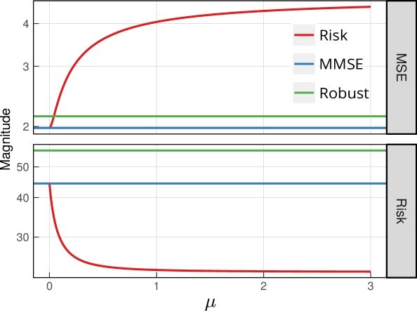
Figure 2: Mean squared error and risk for different values of $\mu$ in the state-dependent noise scenario.

We evaluate the behavior of the estimator in (23) in two different scenarios. The first consists of the problem of estimating an exponentially distributed hidden state $X$, $\mathbb{E}\{X\}=2$, from the observation $Y=X+v$, where $v$ is a zero-mean Gaussian random variable independent of $X$ whose variance is given by $\mathbb{E}\{v^{2}\}=9X^{2}$; in this case, $v$ constitutes a state-dependent noise. In the second scenario, the goal is to jointly estimate the random vector $X=\left[z\ \ h\right]^{T}$ from the observation $Y=hz+w$, where $z$ is a zero-mean Gaussian random variable with variance $\mathbb{E}\{z^{2}\}=2$, $h$ has a Rayleigh distribution with rate $2$, and $w$ is a zero-mean Gaussian noise with variance $\mathbb{E}\{w^{2}\}=10^{-1}$. This scenario is prototypical for estimation problems in communications, where $z$ is the signal of interest and $h$ represents the channel fading. Throughout the simulations, we also show results for the risk-neutral MMSE estimator and the Minimum Mean Absolute Error (MMAE) estimator, or, equivalently, the conditional median relative to the respective observations, the latter being used as an example of a robust location parameter estimator.

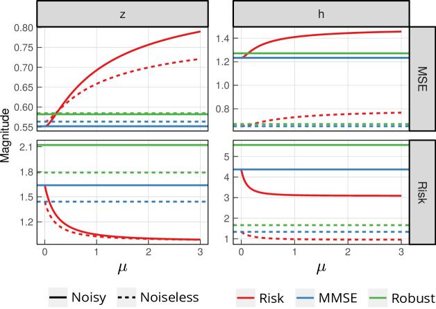
Figure 3: Mean squared error and risk for different values of $\mu$ in the communication scenario.

In Fig. 1, we saw that the risk-aware estimator yields larger estimates than the MMSE estimator, in order to account for the certain statistical ambiguities of the state-dependent noise model. Though this difference may seem extreme in some instances, e.g., for small values of $Y$ (as in Fig. 1), it is in fact quite effective in reducing the conditional variance. Indeed, for $Y=0.1$, the risk-aware estimator in Fig. 1 optimally reduces the (conditional) risk by approximately $26\%$ as compared to the risk of the risk-neutral estimator, and this is achieved by sacrificing average performance, also by a factor of $26\%$. Of course, this is only one of the operation points of the risk-aware estimator. In Fig. 2, we show results for different values of $\mu$, where we average over the distribution of $Y$. Observe that the risk-aware estimator obtained using the constrained optimization problem (2) achieves a sharp trade-off between average performance (that is, mean squared error) and risk, which can be tuned according to the needs of the application. Additionally, note that the decrease in risk is considerably faster than the increase in MSE.

Interestingly, a similar phenomenon is observed in the communication scenario (Fig. 3). Again, the risk-aware estimator displays a much faster initial rate of decrease with respect to $\mu$ than the rate at which the MSE increases. This is more pronounced in the estimation of the component $z$, for which the risk-aware estimator can provide reductions of almost $60\%$ in risk for a $35\%$ increase in average squared error. Note that, as per Theorem 4, the Gaussian noise has indeed no bearing on risk-awareness, as evidenced by the performance in the noiseless case, i.e., for $w=0$ (dashed lines). To achieve the behavior of Fig. 3, the risk-aware estimator overestimates both $z$ and $h$ as compared to the MMSE estimator, as illustrated in Fig. 4. In fact, for small values of $Y$, the former hedges against the event of a deep fade ($h\approx 0$) by maintaining its estimates for $z$ away from zero.

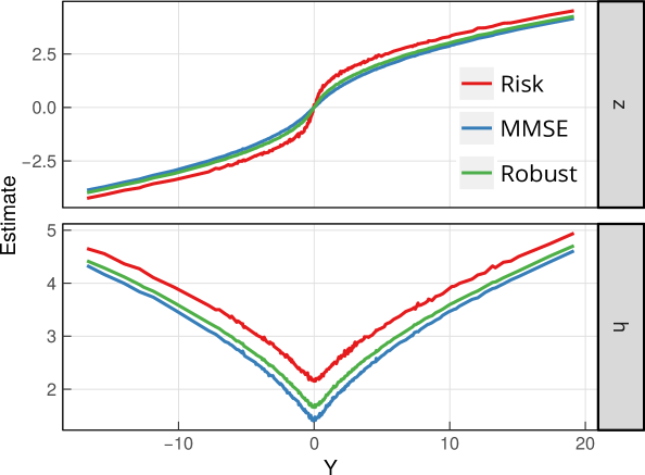
Figure 4: Risk-aware, MMSE, and robust estimates of $z$ and $h$ in the communication scenario for different values of $Y$.

6 Conclusions

We derived a risk-aware MMSE estimator that accounts for statistical model volatility by hedging against extreme losses. We did so by formulating a Bayesian risk-aware MMSE estimation problem that minimizes squared errors on average, subject to an explicit tolerance on their expected predictive variance. We then showed that this problem admits a analytical solution under mild moment boundedness assumptions, and results in a risk-aware, biased nonlinear MMSE estimator. The effectiveness of our approach was confirmed via several numerical simulations. Future work includes further analysis of the statistical properties of the proposed estimator, as well as study of other constrained risk-aware formulations.

References

- [1] Anders Ahlén, Johan Akerberg, Markus Eriksson, A L F J Isaksson, Takuya Iwaki, Karl Henrik Johansson, Steffi Knorn, Thomas Lindh, and Henrik Sandberg, “Toward wireless control in industrial process automation: A case study at a paper mill,” Control Systems, IEEE, vol. 39, no. 5, pp. 36–57, 2019.
- [2] Sergio Bruno, Shabbir Ahmed, Alexander Shapiro, and Alexandre Street, “Risk neutral and risk-averse approaches to multistage renewable investment planning under uncertainty,” European Journal of Operational Research, vol. 250, no. 3, pp. 979–989, May 2016.
- [3] Somayeh Moazeni, Warren B. Powell, and Amir H. Hajimiragha, “Mean-conditional value-at-risk optimal energy storage operation in the presence of transaction costs,” IEEE Transactions on Power Systems, vol. 30, no. 3, pp. 1222–1232, May 2015.
- [4] Harry Markowitz, “Portfolio selection,” The Journal of Finance, vol. 7, no. 1, pp. 77–91, Mar. 1952.
- [5] Hans Föllmer and Alexander Schied, “Convex measures of risk and trading constraints,” Finance and Stochastics, vol. 6, no. 4, pp. 429–447, Oct. 2002.
- [6] Danjue Shang, Victor Kuzmenko, and Stan Uryasev, “Cash flow matching with risks controlled by buffered probability of exceedance and conditional value-at-risk,” Annals of Operations Research, vol. 260, no. 1-2, pp. 501–514, Jan. 2018.
- [7] Sung-Kyun Kim, Rohan Thakker, and Ali-akbar Agha-mohammadi, “Bi-directional value learning for risk-aware planning under uncertainty,” IEEE Robotics and Automation Letters, vol. 4, no. 3, pp. 2493–2500, July 2019.
- [8] Arvind A. Pereira, Jonathan Binney, Geoffrey A. Hollinger, and Gaurav S. Sukhatme, “Risk-aware path planning for autonomous underwater vehicles using predictive ocean models,” Journal of Field Robotics, vol. 30, no. 5, pp. 741–762, Sept. 2013.
- [9] Amrit Singh Bedi, Alec Koppel, and Ketan Rajawat, “Nonparametric compositional stochastic optimization,” arXiv preprint, arXiv:1902.06011, Feb. 2019.
- [10] Wann-Jiun Ma, Chanwook Oh, Yang Liu, Darinka Dentcheva, and Michael M. Zavlanos, “Risk-averse access point selection in wireless communication networks,” IEEE Transactions on Control of Network Systems, vol. 5870, no. c, pp. 1–1, 2018.
- [11] Prashanth L. A. and Michael Fu, “Risk-sensitive reinforcement learning: A constrained optimization viewpoint,” arXiv preprint, arXiv:1810.09126, Oct. 2018.
- [12] Adrian Rivera Cardoso and Huan Xu, “Risk-averse stochastic convex bandit,” in International Conference on Artificial Intelligence and Statistics, Apr. 2019, vol. 89, pp. 39–47.
- [13] Wenjie Huang and William B. Haskell, “Risk-aware q-learning for markov decision processes,” in 2017 IEEE 56th Annual Conference on Decision and Control, CDC 2017. Dec. 2018, vol. 2018-Janua, pp. 4928–4933, IEEE.
- [14] Daniel R. Jiang and Warren B. Powell, “Risk-averse approximate dynamic programming with quantile-based risk measures,” Mathematics of Operations Research, vol. 43, no. 2, pp. 554–579, Nov. 2018.
- [15] Dionysios S. Kalogerias and Warren B. Powell, “Recursive optimization of convex risk measures: Mean-semideviation models,” arXiv preprint, arXiv:1804.00636, Apr. 2018.
- [16] Aviv Tamar, Yinlam Chow, Mohammad Ghavamzadeh, and Shie Mannor, “Sequential decision making with coherent risk,” IEEE Transactions on Automatic Control, vol. 62, no. 7, pp. 3323–3338, July 2017.
- [17] Constantine Alexander Vitt, Darinka Dentcheva, and Hui Xiong, “Risk-averse classification,” Annals of Operations Research, Aug. 2019.
- [18] Lifeng Zhou and Pratap Tokekar, “An approximation algorithm for risk-averse submodular optimization,” arXiv preprint, arXiv:1807.09358, July 2018.
- [19] Alexander Shapiro, Darinka Dentcheva, and Andrzej Ruszczyński, Lectures on Stochastic Programming: Modeling and Theory, Society for Industrial and Applied Mathematics, 2nd edition, 2014.
- [20] R. Tyrrell Rockafellar and Stanislav Uryasev, “Optimization of conditional value-at-risk,” Journal of Risk, vol. 2, pp. 21–41, 1997.
- [21] P Whittle, “Risk-sensitive linear/quadratic/gaussian control,” Adv. Appl. Prob, vol. 13, pp. 764–777, 1981.
- [22] J.L. Speyer, C.-H. Fan, and R.N. Banavar, “Optimal stochastic estimation with exponential cost criteria,” in Proceedings of the 31st IEEE Conference on Decision and Control. Aug. 1992, pp. 2293–2298, Institute of Electrical and Electronics Engineers (IEEE).
- [23] J. B. Moore, R. J. Elliott, and S. Dey, “Risk-sensitive generalizations of minimum variance estimation and control,” Journal of Mathematical Systems, Estimation, and Control, vol. 7, no. 1, pp. 123–126, 1997.
- [24] Subhrakanti Dey and John B. Moore, “Risk-sensitive filtering and smoothing via reference probability methods,” IEEE Transactions on Automatic Control, vol. 42, no. 11, pp. 1587–1591, 1997.
- [25] Subhrakanti Dey and John B. Moore, “Finite-dimensional risk-sensitive filters and smoothers for discrete-time nonlinear systems,” IEEE Transactions on Automatic Control, vol. 44, no. 6, pp. 1234–1239, 1999.
- [26] David G. Luenberger, Optimization by Vector Space Methods, Wiley, 1968.
- [27] R. T. Rockafellar and R. J-B Wets, Variational Analysis, vol. 317, Springer Science & Business Media, 2004.