At the Corner of Space and Time

Barak Shoshany

Waterloo, Ontario, Canada, 2019

© Barak Shoshany 2019

Examining Committee Membership

The following served on the Examining Committee for this thesis. The decision of the Examining Committee is by majority vote.

External Examiner:	Karim Noui
	Associate Professor
	University of Tours

Supervisors:	Laurent Freidel
	Faculty
	Perimeter Institute for Theoretical Physics
	Robert Myers
	Faculty
	Perimeter Institute for Theoretical Physics

Internal Members:	Robert Mann
	Professor
	University of Waterloo
	John Moffat
	Professor Emeritus
	University of Toronto

Internal-External Member:	Florian Girelli
	Associate Professor
	University of Waterloo

Author’s Declaration

This thesis consists of material all of which I authored or co-authored: see Statement of Contributions included in the thesis. This is a true copy of the thesis, including any required final revisions, as accepted by my examiners.

I understand that my thesis may be made electronically available to the public.

Statement of Contributions

This thesis is based on the papers [1], co-authored with Laurent Freidel and Florian Girelli, the papers [2, 3], of which I am the sole author, and additional unpublished material, of which I am the sole author.

Abstract

We perform a rigorous piecewise-flat discretization of classical general relativity in the first-order formulation, in both 2+1 and 3+1 dimensions, carefully keeping track of curvature and torsion via holonomies. We show that the resulting phase space is precisely that of spin networks, the quantum states of discrete spacetime in loop quantum gravity, with additional degrees of freedom called edge modes, which control the gluing between cells. This work establishes, for the first time, a rigorous proof of the equivalence between spin networks and piecewise-flat geometries with curvature and torsion degrees of freedom. In addition, it demonstrates that careful consideration of edge modes is crucial both for the purpose of this proof and for future work in the field of loop quantum gravity. It also shows that spin networks have a dual description related to teleparallel gravity, where gravity is encoded in torsion instead of curvature degrees of freedom. Finally, it sets the stage for collaboration between the loop quantum gravity community and theoretical physicists working on edge modes from other perspectives, such as quantum electrodynamics, non-abelian gauge theories, and classical gravity.

Acknowledgments

Note: Wherever a list of names is provided in this section, it is always ordered alphabetically by last name.

First and foremost, I would like to thank my supervisor, Laurent Freidel, for giving me the opportunity to study at the wonderful Perimeter Institute and to write both my master’s thesis and my PhD thesis under his guidance, and for supporting me and believing in me throughout the last 5 years, even when I didn’t believe in myself. His deep physical intuition has inspired me countless times. He constantly challenged me and pushed me to expand my horizons in both mathematics and physics, to improve my research skills as well as my presentation and communication skills, and to be a better scientist. Needless to say, this thesis would not have existed without him.

I am also incredibly thankful to Florian Girelli for collaborating with me on this research and for his continued assistance and helpful advice during the last 3 years. Our frequent meetings and stimulating discussions have been an invaluable resource, and provided me not only with the knowledge and insight necessary to succeed in writing this thesis, but also with the motivation to overcome the many obstacles that are an inevitable part of research.

I thank my examination committee members Robert Mann, John Moffat, and Robert Myers, as well as the external examiner Karim Noui, for taking time out of their very busy schedules to read this thesis. I hope I have made it readable and interesting enough for this to be a pleasant experience.

Special thanks go to Wolfgang Wieland, who patiently provided clear and detailed explanations of complicated concepts in mathematics and physics whenever I needed his help, and to Marc Geiller, Hal Haggard, Seyed Faroogh Moosavian, Yasha Neiman, Kasia Rejzner, Aldo Riello, and Vasudev Shyam for very helpful discussions.

I thank my students from the International Summer School for Young Physicists (ISSYP), the Perimeter Institute Undergraduate Summer Program, and the Perimeter Scholars International (PSI) Program over the last 5 years for consistently asking challenging questions, which forced me to think outside the box and improve myself and my knowledge in many different ways.

Sharing my knowledge of mathematics and physics in the numerous teaching and outreach events, programs, and initiatives at Perimeter Institute has served as a constant reminder of why I got into science in the first place. For that privilege, I owe my gratitude to Greg Dick, Kelly Foyle, Damian Pope, Angela Robinson, Marie Strickland, and Tonia Williams from Perimeter Institute’s outreach department.

I owe great thanks to Dan Wohns and Gang Xu for teaching me during my studies in the PSI program, for choosing me to serve as a teaching assistant in the PSI quantum field theory and string theory courses, for introducing me to many fun board games, and for inviting me to conduct the Perimeter Institute Orchestra. I also thank the members of the orchestra for agreeing to play my composition, Music at the Planck Scale, which was no easy task by any means. Working on this and other music projects has made my time at Perimeter Institute so much more fun!

I am grateful to Perimeter Institute’s Academic Programs Manager, Debbie Guenther, for being so amazingly helpful and supportive in many different logistical hurdles throughout both my master’s and PhD studies. I also thank the staff at Perimeter Institute’s Black Hole Bistro, and in particular Dan Lynch and Olivia Taylor, for providing me with delicious food on a daily basis for 5 years, and for tolerating my many unusual requests.

I would not have been where I am today without my parents, Avner and Judith Shoshany, who, ever since I was born, have constantly empowered me to follow my dreams, no matter how crazy, impossible, or impractical they were, and always did everything they could in order to help me achieve those dreams and more. They have my eternal gratitude and appreciation.

Finally, I would like to thank all of my friends, and especially Jacob Barnett, Juan Cayuso, Daniel Guariento, Fiona McCarthy, Yasha Neiman, Kasia Rejzner, Vasudev Shyam, Matthew VonHippel, Dan Wohns, and Gang Xu, for much-needed distractions from the frequent frustrations of graduate school over the last 5 years (especially in the form of playing games or watching stand-up comedy), for providing unconditional emotional support when needed, and/or for patiently listening to my endless complaints.

1 Introduction

1.1 Loop Quantum Gravity

When perturbatively quantizing gravity, one obtains a low-energy effective theory, which breaks down at high energies. There are several different approaches to solving this problem and obtaining a theory of quantum gravity. String theory, for example, attempts to do so by postulating entirely new degrees of freedom, which can then be shown to reduce to general relativity (or some modification thereof) at the low-energy limit. Loop quantum gravity [5] instead tries to quantize gravity non-perturbatively, by quantizing holonomies (or Wilson loops) instead of the metric, in an attempt to avoid the issues arising from perturbative quantization.

The starting point of the canonical version of loop quantum gravity [6] is the reformulation of general relativity as a non-abelian Yang-Mills gauge theory on a spatial slice of spacetime, with the gauge group $\mathrm{SU}\left(2\right)$ related to spatial rotations, the Yang-Mills connection $\mathbf{A}$ related to the usual connection and extrinsic curvature, and the “electric field” $\mathbf{E}$ related to the metric (or more precisely, the frame field). Once gravity is reformulated in this way, one can utilize the existing arsenal of techniques from Yang-Mills theory, and in particular lattice gauge theory, to tackle the problem of quantum gravity [7].

This theory is quantized by considering graphs, that is, sets of nodes connected by links. One defines holonomies, or path-ordered exponentials of the connection, along each link. The curvature on the spatial slice can then be probed by looking at holonomies along loops on the graph. Without going into the technical details, the general idea is that if we know the curvature inside every possible loop, then this is equivalent to knowing the curvature at every point.

The kinematical Hilbert space of loop quantum gravity is obtained from the set of all wave-functionals for all possible graphs, together with an appropriate $\mathrm{SU}\left(2\right)$-invariant and diffeomorphism-invariant inner product. The physical Hilbert space is a subset of the kinematical one, containing only the states invariant under all gauge transformations – or in other words, annihilated by all of the constraints. Since gravity is a totally constrained system – in the Hamiltonian formulation, the action is just a sum of constraints – a quantum state annihilated by all of the constraints is analogous to a metric which solves Einstein’s equations in the classical Lagrangian formulation.

Specifically, to get from the kinematical to the physical Hilbert space, three steps must be taken:

1. First, we apply the Gauss constraint to the kinematical Hilbert space. Since the Gauss constraint generates $\mathrm{SU}\left(2\right)$ gauge transformation, we obtain a space of $\mathrm{SU}\left(2\right)$-invariant states, called spin network states [8], which are the graphs mentioned above, but with their links colored by irreducible representations of $\mathrm{SU}\left(2\right)$, that is, spins $j\in\left\{\frac{1}{2},1,\frac{3}{2},2,\ldots\right\}$.

2. Then, we apply the spatial diffeomorphism constraint. We obtain a space of equivalence classes of spin networks under spatial diffeomorphisms, a.k.a. knots. These states are now abstract graphs, not localized in space. This is analogous to how a classical geometry is an equivalence class of metrics under diffeomorphisms.

3. Lastly, we apply the Hamiltonian constraint. This step is still not entirely well-understood, and is one of the main open problems of the theory.

One of loop quantum gravity’s most celebrated results is the existence of area and volume operators. They are derived by taking the usual integrals of area and volume forms and promoting the “electric field” $\mathbf{E}$, which is conjugate to the connection $\mathbf{A}$, to a functional derivative $\delta/\delta\mathbf{A}$. The spin network states turn out to be eigenstates of these operators, and they have discrete spectra which depend on the spins of the links. This means that loop quantum gravity contains a quantum geometry, which is a feature one would expect a quantum theory of spacetime to have. It also hints that spacetime is discrete at the Planck scale.

However, it is not clear how to rigorously define the classical geometry related to a particular spin network state. In this thesis, we will try to answer that question.

1.2 Teleparallel Gravity

The theory of general relativity famously describes gravity as a result of the curvature of spacetime itself. Furthermore, the geometry of spacetime is assumed to be torsionless by employing the Levi-Civita connection, which is torsionless by definition. While this is the most popular formulation, there exists an alternative but mathematically equivalent formulation called teleparallel gravity [9, 10, 11], differing from general relativity only by a boundary term. In this formulation, one instead uses the Weitzenböck connection, which is flat by definition. The gravitational degrees of freedom are then encoded in the torsion of the spacetime geometry.

In the canonical version of loop quantum gravity, as we mentioned above, one starts by rewriting general relativity in the Hamiltonian formulation using the Ashtekar variables. One finds a fully constrained system, that is, the Hamiltonian is simply a sum of constraints. In 2+1 spacetime dimensions, where gravity is topological [12], there are two such constraints:

• The Gauss (or torsion) constraint, which imposes zero torsion everywhere,

• The curvature (or flatness) constraint, which imposes zero curvature everywhere.

After imposing both constraints, we will obtain the physical Hilbert space of the theory. It does not matter which constraint is imposed first, since the resulting physical Hilbert space will be the same. However, on a more conceptual level, the first constraint that we impose is used to define the kinematics of the theory, while the second constraint will encode the dynamics. Thus, it seems natural to identify general relativity with the quantization in which the Gauss constraint is imposed first, and teleparallel gravity with that in which the curvature constraint is imposed first.

Indeed, in loop quantum gravity, which is a quantization of general relativity, the Gauss constraint is imposed first, as detailed in the previous section. This is true in both 2+1 and 3+1 dimensions. In 2+1D, the curvature constraint is imposed at the dynamical level in order to obtain the Hilbert space of physical states. In 3+1D there is no curvature constraint – the curvature is, in general, not flat. One instead imposes the diffeomorphism and Hamiltonian constraints to get the physical Hilbert space, but the Gauss constraint is still imposed first.

In [13], an alternative choice was suggested where the order of constraints, in 2+1D, is reversed. The curvature constraint is imposed first by employing the group network basis of translation-invariant states, and the Gauss constraint is the one which encodes the dynamics. This dual loop quantum gravity quantization is the quantum counterpart of teleparallel gravity, and could be used to study the dual vacua proposed in [14, 15].

In this thesis, we will only deal with the classical theory. We will show how, by discretizing the phase space of continuous gravity in the first-order formulation (and with the Ashtekar variables in 3+1D), one obtains a spectrum of discrete phase spaces, one of which is the classical version of spin networks [16] and the other is a dual formulation (“dual loop gravity”), which may be interpreted as the classical version of the group network basis, and is intuitively related to teleparallel gravity. The latter case was first studied in [17], but only in 2+1 dimensions, and only in the simple case where there are no curvature or torsion excitations.

Another phase space of interest in the spectrum discussed above is a mixed phase space, containing both loop gravity and its dual. In 2+1D it is intuitively related to Chern-Simons theory [18], as we will motivate below. In this case our formalism is related to existing results [19, 20, 21, 22, 23, 24, 25].

1.3 Quantization, Discretization, Subdivision, and Truncation

One of the key challenges in trying to define a theory of quantum gravity at the quantum level is to find a regularization that does not drastically break the fundamental symmetries of the theory. This is a challenge in any gauge theory, but gravity is especially challenging, for two reasons. First, one expects that the quantum theory possesses a fundamental length scale; and second, the gauge group contains diffeomorphism symmetry, which affects the nature of the space on which the regularization is applied.

In gauge theories such as quantum chromodynamics (QCD), the only known way to satisfy these requirements, other than gauge-fixing before regularization, is to put the theory on a lattice, where an effective finite-dimensional gauge symmetry survives at each scale. One would like to devise such a scheme in the gravitational context as well. In this thesis, we develop a step-by-step procedure to achieve this, exploiting, among other things, the fact that first-order gravity in 2+1 dimensions, as well as gravity in 3+1 dimensions with the Ashtekar variables, closely resembles other gauge theories. We find not only the spin network or holonomy-flux phase space, which is what we initially expected, but also additional particle-like or string-like degrees of freedom coupled to the curvature and torsion.

As explained above, in canonical loop quantum gravity (LQG), one can show that the geometric operators possess a discrete spectrum. This is, however, only possible after one chooses the quantum spin network states to have support on a graph. Spin network states can be understood as describing a quantum version of discretized spatial geometry [5], and the Hilbert space associated to a graph can be related, in the classical limit, to a set of discrete piecewise-flat geometries [26, 16].

This means that the LQG quantization scheme consists at the same time of a quantization and a discretization; moreover, the quantization of the geometric spectrum is entangled with the discretization of the fundamental variables. It has been argued that it is essential to disentangle these two different features [27], especially when one wants to address dynamical issues.

In [27, 28], it was suggested that one should understand the discretization as a two-step process: a subdivision followed by a truncation. In the first step one subdivides the systems into fundamental cells, and in the second step one chooses a truncation of degrees of freedom in each cell, which is consistent with the symmetries of the theory. By focusing first on the classical discretization, before any quantization takes place, several aspects of the theory can be clarified. Let us mention some examples:

• This discretization scheme allows us to study more concretely how to recover the continuum geometry out of the classical discrete geometry associated to the spin networks [27, 28]. In particular, since the discretization is now understood as a truncation of the continuous degrees of freedom, it is possible to associate a continuum geometry to the discrete data.

• It provides a justification for the fact that, in the continuum case, the momentum variables are equipped with a vanishing Poisson bracket, whereas in the discrete case, the momentum variables do not commute with each other [27, 17, 14]. These variables need to be dressed by the gauge connection, as we will explain in the next section, and are now understood as charge generators [29].

• As detailed above, our discretization scheme permits the discovery and study of a dual formulation of loop gravity, both in 2+1 and 3+1 dimensions.

The separation of discretization into two distinct steps in our formalism work as follows. First we perform a subdivision, or decomposition into subsystems. More precisely, we define a cellular decomposition on our 2D or 3D spatial manifold, where the cells can be any (convex) polygons or polyhedra respectively. This structure has a dual structure, which as we will see, is the spin network graph, with each cell dual to a node, and each element on the boundary of the cell (edge in 2+1D, side in 3+1D) dual to a link connected to that node.

Then, we perform a truncation, or coarse-graining of the subsystems. In this step, we assume that there is arbitrary curvature and torsion inside each loop of the spin network. We then “compress” the information about the geometry into singular codimension-2 excitations. In 2+1D it will be stored in a 0-dimensional (point particle) excitation, while in 3+1D it will be stored in a 1-dimensional (string) excitation. Crucially, since the only way to probe the geometry is by looking at the holonomies on the loops of the spin network, the observables before and after this truncation are the same.

Another way to interpret this step is to instead assume that spacetime is flat everywhere, with matter sources being distributive, i.e., given by Dirac delta functions, which then generate singular curvature and torsion by virtue of the Einstein equation. We interpret these distributive matter sources as point particles in 2+1D or strings in 3+1D, and this is entirely equivalent to truncating a continuous geometry, since holonomies cannot distinguish between continuous and distributive geometries.

Once we performed subdivision and truncation, we can now define discrete variables on each cell and integrate the continuous symplectic potential in order to obtain a discrete potential, which represents the discrete phase space. In this step, we will see that the mathematical structures we are using conspire to cancel many terms in the potential, allowing us to fully integrate it.

1.4 Edge Modes

In the subdivision process described above, some of the bulk degrees of freedom are replaced by edge mode degrees of freedom, which play a key role in the construction of the full phase space and our understanding of symmetry. This happens because dealing with subsystems in a gauge theory requires special care with regards to boundaries, where gauge invariance is naively broken, and thus additional degrees of freedom must be added in order to restore it. These new degrees of freedom transform non-trivially under new symmetry transformations located on the edges and/or corners; we will usually ignore this distinction and just call them “edge modes”. The process of subdivision therefore requires a canonical extension of the phase space, and converting some momenta into non-commutative charge generators.

The general philosophy is presented in [29] and exemplified in the 3+1D gravity context in [30, 31, 32]. An intuitive reason behind this fundamental mechanism is also presented in [33] and the general idea is, in a sense, already present in [34]. In the 2+1D gravity context, the edge modes have been studied in great detail in [4, 35]. This phenomenon even happens when the boundary is taken to be infinity [36], where these new degrees of freedom are called soft modes.

These extra degrees of freedom, which possess their own phase space structure and appear as dressings of the gravitationally charged observables, affect the commutation relations of the dressed observables. In a precise sense, this is what happens with the fluxes in loop gravity: the “discretized” fluxes are dressed by the connection degrees of freedom, implying a different Poisson structure compared to the continuum ones. A nice continuum derivation of this fact is given in [37].

Once this subdivision and extension of the phase space are done properly, one has to understand the gluing of subregions as the fusion of edge modes across the boundaries. If the boundary is trivial, this fusion merely allows us to extend gauge-invariant observables from one region to another. However, when several boundaries meet at a corner, there is now the possibility to have residual degrees of freedom that come from this fusion.

We witness exactly this phenomenon at the corners of our cellular decomposition – vertices in 2+1D or edges in 3+1D – where new degrees of freedom, in addition to the usual loop gravity ones, are found after regluing. As we will see below, the edge modes at the boundaries of the cells in our cellular decomposition – edges in 2+1D or sides in 3+1D – will cancel with the edge modes on the boundaries of the adjacent cells. However, the modes at the corners do not have anything to cancel with. These degrees of freedom will thus survive the discretization process. In 2+1D, they introduce a particle-like phase space [38, 39], while in 3+1D, we interpret them as cosmic strings [40].

One might expect that the geometry will be encoded in the constraints alone, by imposing, roughly speaking, that a loop of holonomies sees the curvature inside it and a loop of fluxes sees the torsion inside it. As we will see, while the constraints do indeed encode the geometry, the presence of the edge and corner modes is the reason for the inclusion of the curvature and torsion themselves as additional phase space variables.

After we have proven our results in 2+1D a very careful and rigorous way, by regularizing the singularities at the vertices, we will derive them again in a different and shorter way. In this alternative calculation, we will show that when calculating the symplectic potential, the terms at the corners (that is, the vertices) completely vanish if there are no curvature or torsion excitations at the vertices. However, if such excitations do exist, the corner terms instead turn out to add up in exactly the right way to produce the additional phase space variables we found before, in our more complicated calculation.

In the 3+1D case, many additional complications occur that were not present in 2+1D, and therefore we will jump right to the alternative analysis. A major difference, as mentioned above, is that the sources of curvature and torsion will now be 1-dimensional strings, rather than 0-dimensional point particles as we had in 2+1D. However, the curvature and torsion will nonetheless still be detected by loops of holonomies, as in the 2+1D case. Furthermore, we will discover that, analogously, one can isolate the terms at the corners (which are now edges), and they vanish unless the edges possess curvature or torsion excitations. In fact, interestingly, we will obtain the exact same discrete phase space as in the 2+1D case: a spin network coupled to edge modes.

As we alluded in the beginning of this section, the edge modes come equipped with new symmetries, which did not exist in the continuum theory. We will show below that multiplying the discrete holonomies by group elements from the right (right translations) corresponds to the usual gauge transformation. The new symmetries we discovered are obtained by instead multiplying from the left (left translations). These symmetries leave the continuous connection invariant, and therefore correspond to completely new degrees of freedom in the discrete variables, which did not exist in the continuum. When the edge modes are “frozen”, meaning that we choose a particular value for them (which can be, without loss of generality, the identity), the new symmetries are broken, and the phase space reduces to the usual loop gravity phase space (or its dual), without these additional degrees of freedom.

The conceptual shift towards an edge mode interpretation provides a different paradigm to explore some of the key questions of loop quantum gravity. For example, the notion of the continuum limit (in a 3+1-dimensional theory) attached to subregions could potentially be revisited and clarified in light of this new interpretation, and related to the approach developed in [41, 42]. It also strengthens, in a way, the spinor approach to LQG [43, 44, 45], which allows one to recover the LQG formalism from spinors living on the nodes of the graph. These spinors can be seen as a different parametrization of the edge modes, in a similar spirit to [46, 47].

Edge modes have recently been studied for the purpose of making proper entropy calculations in gauge theory or, more generally, defining local subsystems [34]. Their use could provide some new guidance for understanding the concept of entropy in loop quantum gravity. They are also relevant to the study of specific types of boundary excitations in condensed matter [48], which could generate some interesting new directions to explore in LQG, as in [49, 41]. Very recently, [50, 51] showed that one can view the constraints of 3+1D gravity in the Ashtekar formulation as a conservation of edge charges, thus uncovering a new conceptual framework.

1.5 Comparison to Previous Work

1.5.1 Combinatorial Quantization of 2+1D Gravity

Discretization (and quantization) of 2+1D gravity was already performed some time ago with the combinatorial quantization of Chern-Simons theory [19, 20, 21, 22]. While our results in 2+1D should be equivalent to this formulation, they also add some new and important insights.

First, we work directly with the gravitational variables and the associated geometric quantities, such as torsion and curvature. Our procedure describes clearly how such objects should be discretized, which is not obvious in the Chern-Simons picture; see for example [52] where the link between the combinatorial framework and LQG was explored.

Second, we are using a different discretization procedure than the one used in the combinatorial approach. Instead of considering the reduced graph, we use the full graph to generate the spin network, and assume that the equations of motion are satisfied in the cells dual to the spin network.

Finally, we will show in detail that our discretization scheme applies, with the necessary modifications, to the 3+1D case as well, unlike the combinatorial approach.

1.5.2 2+1D Gravity, Chern-Simons Theory, and Point Particles

In [53], it is emphasized that Chern-Simons theory and Einstein gravity are in fact not equivalent up to a boundary term, with the difference being that in Einstein gravity the fame field $\mathbf{e}$ is required to be invertible, unlike in Chern-Simons theory. We will always assume in this thesis that the frame field is in fact invertible, and often use the inverse frame field as part of our derivation, but this will not be a problem since we are only interested in the gravity case anyway, and in particular in the generalization to 3+1D gravity, where the frame field is invertible as well.

The same author, in [54], analyzed the phase space of a toy model of discretized 2+1D gravity with point particles, which is similar to the one we will consider here. In particular, Chapter 4 of [54] obtains results that are remarkably similar to some of ours. The symplectic potential found in Eq. (4.48) of [54] is reminiscent of our Eq. (8.13) with $\lambda=1$, which, as we will show, is the dual (or teleparallel) loop gravity polarization, although there it is not interpreted as such.

Another interesting treatment of point particles in 2+1D gravity was given in [55], where the coupling to spinning particles and the relation with the spin foam scalar product were examined, and in [56], where the relation between canonical loop quantization and spin foam quantization in 3+1D was established. Finally, in [57] it was shown, in the context of the Ponzano-Regge model of 2+1D quantum gravity, that particles arise as curvature defects, which is indeed what we will see in this thesis; furthermore, it was shown this model is linked to the quantization of Chern-Simons theory.

1.6 Outline

This thesis is meant to be as self-contained as possible, with all the necessary background for each chapter provided in full in the preceding chapters. First, in Chapter 2, we provide a comprehensive list of basic definitions, notations, and conventions which will be used throughout the thesis. It is highly recommended that the reader not skip this chapter, as some of our notation is slightly non-standard. Then we begin the thesis itself, which consists of four parts.

Part I presents 2+1-dimensional general relativity in the continuum. Chapter 3 consists of a self-contained derivation of Chern-Simons theory and, from it, 2+1-dimensional gravity in both the Lagrangian and Hamiltonian formulations. It also introduces the teleparallel formulation. Chapter 4 then discusses Euclidean gauge transformations and the role of edge modes. Finally, in Chapter 5 we introduce matter degrees of freedom in the form of point particles.

In Part II, we discretize the theory presented in Part I. In Chapter 6, we describe the discrete geometry we will be using. We define the cellular decomposition and the dual spin network, including a derivation of the spin network phase space, and then show how the continuous geometry is truncated using holonomies. We also introduce the continuity conditions relating the variables between different cells. Chapter 7 then discusses gauge transformations and symmetries in the discrete setting, which includes new symmetries which did not exist in the continuous version. In Chapter 8 we rigorously discretize the symplectic potential of the continuous theory, and show how, from the continuous gravity phase space, we obtain both the spin network and edge mode phase spaces. Chapters 9 and 10 then analyzes, in elaborate detail, the constraints obtained in the discrete theory and the symmetries they generate. Finally, in Chapter 11 we repeat the derivation of Chapter 8 from scratch under much simplifying assumptions.

Part III is the prelude for adapting our results from the toy model of 2+1 dimensions to the physically relevant case of 3+1 spacetime dimensions. In Chapter 12 we provide a detailed and self-contained derivation of the Ashtekar variables and the loop gravity Hamiltonian action, including the constraints. Special care is taken to write everything in terms of index-free Lie-algebra-valued differential forms, as we did in the 2+1-dimensional case, which – in addition to being more elegant – will greatly simplify our derivation. Chapter 13 then introduces matter degrees of freedom, this time in the form of cosmic strings, mirroring our discussion of point particles in the 2+1-dimensional case.

Finally, in Part IV we discretize the 3+1-dimensional theory. In Chapter 14 we introduce the discrete geometry, where now the cells are 3-dimensional, and discuss the truncation of the geometry using holonomies. In Chapter 15 we perform a calculation analogous to the one we performed in Chapters 8 and later in 11, although it is of course now more involved. We show that, in the 3+1-dimensional case as well, the spin network phase space coupled to edge modes is obtained from the continuous phase space. Moreover, we obtain a spectrum of polarizations which includes a dual theory, as in the 2+1-dimensional case. Chapter 16 summarizes the results of this thesis and presents several avenues for potential future research.

2 Basic Definitions, Notations, and Conventions

The following definitions, notations, and conventions will be used throughout the thesis.

2.1 Lie Group and Algebra Elements

Let $G$ be a Lie group, let $\mathfrak{g}$ be its associated Lie algebra, and let $\mathfrak{g}^{*}$ be the dual to that Lie algebra. The cotangent bundle of $G$ is the Lie group $T^{*}G\cong G\ltimes\mathfrak{g}^{*}$, where $\ltimes$ is the semidirect product, and it has the associated Lie algebra $\mathfrak{g}\oplus\mathfrak{g}^{*}$. We assume that this group is the Euclidean or Poincaré group, or a generalization thereof, and its algebra takes the form

$$\left[\mathbf{P}_{i},\mathbf{P}_{j}\right]=0,\qquad\left[\mathbf{J}_{i},\mathbf{J}_{j}\right]=f_{ij}{}^{k}\mathbf{J}_{k},\qquad\left[\mathbf{J}_{i},\mathbf{P}_{j}\right]=f_{ij}{}^{k}\mathbf{P}_{k},$$ (2.1)

where:

• $f_{ij}{}^{k}$ are the structure constants, which satisfy anti-symmetry $f_{ij}{}^{k}=-f_{ji}{}^{k}$ and the Jacobi identity $f_{[ij}{}^{l}f_{k]l}{}^{m}=0$.

• $\mathbf{J}_{i}\in\mathfrak{g}$ are the rotation generators,

• $\mathbf{P}_{i}\in\mathfrak{g}^{*}$ are the translation generators,

• The indices $i,j,k$ take the values $0,1,2$ in the 2+1D case, where they are internal spacetime indices, and $1,2,3$ in the 3+1D case, where they are internal spatial indices.

Usually in the loop quantum gravity literature we take $G=\mathrm{SU}\left(2\right)$ such that $\mathfrak{g}^{*}=\mathbb{R}^{3}$ and

$$\mathrm{ISU}\left(2\right)\cong\mathrm{SU}\left(2\right)\ltimes\mathbb{R}^{3}\cong T^{*}\mathrm{SU}\left(2\right).$$ (2.2)

However, here we will mostly keep $G$ abstract in order for the discussion to be more general.

Throughout this thesis, different fonts and typefaces will distinguish elements of different groups and algebras, or differential forms valued in those groups and algebras, as follows:

• $G\ltimes\mathfrak{g}^{*}$-valued forms will be written in Calligraphic font: $\mathcal{A},\mathcal{B},\mathcal{C},...$

• $\mathfrak{g}\oplus\mathfrak{g}^{*}$-valued forms will be written in bold Calligraphic font: $\boldsymbol{\mathcal{A}},\boldsymbol{\mathcal{B}},\boldsymbol{\mathcal{C}},...$

• $G$-valued forms will be written in regular font: $a,b,c,...$

• $\mathfrak{g}$ or $\mathfrak{g}^{*}$-valued forms will be written in bold font: $\mathbf{a},\mathbf{b},\mathbf{c},...$

2.2 Indices and Differential Forms

Throughout this thesis, we will use the following conventions for indices:

• In the 2+1D case:

  • $\mu,\nu,\ldots\in\left\{0,1,2\right\}$ represent 2+1D spacetime components.

  • $i,j,\ldots\in\left(0,1,2\right)$ represent 2+1D internal / Lie algebra components.

  • $a,b,\ldots\in\left\{1,2\right\}$ represent 2D spatial components: $\overbrace{0,\underbrace{1,2}_{a}}^{\mu}$.

• In the 3+1D case:

  • $\mu,\nu,\ldots\in\left\{0,1,2,3\right\}$ represent 3+1D spacetime components.

  • $A,B,\ldots,I,J,\ldots\in\left(0,1,2,3\right)$ represent 3+1D internal components.

  • $a,b,\ldots\in\left\{1,2,3\right\}$ represent 3D spatial components: $\overbrace{0,\underbrace{1,2,3}_{a}}^{\mu}$.

  • $i,j,\ldots\in\left\{1,2,3\right\}$ represent 3D internal / Lie algebra components: $\overbrace{0,\underbrace{1,2,3}_{i}}^{I}$.

We consider a 2+1D or 3+1D manifold $M$ with topology $\Sigma\times\mathbb{R}$ where $\Sigma$ is a 2 or 3-dimensional spatial manifold and $\mathbb{R}$ represents time. Our metric signature convention is $\left(-,+,+\right)$ or $\left(-,+,+,+\right)$. In index-free notation, we denote a Lie-algebra-valued differential form of degree $p$ (or $p$-form) on $\Sigma$, with one algebra index $i$ and $p$ spatial indices $a_{1},\ldots,a_{p}$, as

$$\mathbf{A}\equiv\frac{1}{p!}A_{a_{1}\cdots a_{p}}^{i}\boldsymbol{\tau}_{i}\thinspace\mathrm{d}x^{a_{1}}\wedge\cdots\wedge\mathrm{d}x^{a_{p}}\in\Omega^{p}\left(\Sigma,\mathfrak{g}\right),$$ (2.3)

where $A_{a_{1}\cdots a_{p}}^{i}$ are the components and $\boldsymbol{\tau}_{i}$ are the generators of the algebra $\mathfrak{g}$ in which the form is valued.

Sometimes we will only care about the algebra index, and write $\mathbf{A}\equiv A^{i}\boldsymbol{\tau}_{i}$ with the spatial indices implied, such that $A^{i}\equiv\frac{1}{p!}A_{a_{1}\cdots a_{p}}^{i}\mathrm{d}x^{a_{1}}\wedge\cdots\wedge\mathrm{d}x^{a_{p}}$ are real-valued $p$-forms. Other times we will only care about the spacetime indices, and write $\mathbf{A}\equiv\frac{1}{p!}\mathbf{A}_{a_{1}\cdots a_{p}}\mathrm{d}x^{a_{1}}\wedge\cdots\wedge\mathrm{d}x^{a_{p}}$ with the algebra index implied, such that $\mathbf{A}_{a_{1}\cdots a_{p}}\equiv A_{a_{1}\cdots a_{p}}^{i}\boldsymbol{\tau}_{i}$ are algebra-valued 0-forms.

2.3 The Graded Commutator

Given any two Lie-algebra-valued forms $\mathbf{A}$ and $\mathbf{B}$ of degrees $\deg\mathbf{A}$ and $\deg\mathbf{B}$ respectively, we define the graded commutator:

$$\left[\mathbf{A},\mathbf{B}\right]\equiv\mathbf{A}\wedge\mathbf{B}-\left(-1\right)^{\deg\mathbf{A}\deg\mathbf{B}}\mathbf{B}\wedge\mathbf{A},$$ (2.4)

which satisfies

$$\left[\mathbf{A},\mathbf{B}\right]=-\left(-1\right)^{\deg\mathbf{A}\deg\mathbf{B}}\left[\mathbf{B},\mathbf{A}\right].$$ (2.5)

If at least one of the forms has even degree, this reduces to the usual anti-symmetric commutator; if we then interpret $\mathbf{A}$ and $\mathbf{B}$ as vectors in $\mathbb{R}^{3}$, then this is none other than the vector cross product $\mathbf{A}\times\mathbf{B}$. Note that $\left[\mathbf{A},\mathbf{B}\right]$ is a Lie-algebra-valued $\left(\deg\mathbf{A}+\deg\mathbf{B}\right)$-form.

The graded commutator satisfies the graded Leibniz rule:

$$\mathrm{d}\left[\mathbf{A},\mathbf{B}\right]=\left[\mathrm{d}\mathbf{A},\mathbf{B}\right]+\left(-1\right)^{\deg\mathbf{A}}\left[\mathbf{A},\mathrm{d}\mathbf{B}\right].$$ (2.6)

In terms of indices, with $\deg\mathbf{A}=p$ and $\deg\mathbf{B}=q$, we have

$$\left[\mathbf{A},\mathbf{B}\right]=\frac{1}{\left(p+q\right)!}\left[\mathbf{A},\mathbf{B}\right]_{a_{1}\cdots a_{p}b_{1}\cdots b_{q}}^{k}\boldsymbol{\tau}_{k}\mathrm{d}x^{a_{1}}\wedge\cdots\wedge\mathrm{d}x^{a_{p}}\wedge\mathrm{d}x^{b_{1}}\wedge\cdots\wedge\mathrm{d}x^{b_{q}},$$ (2.7)

where

$$\left[\mathbf{A},\mathbf{B}\right]_{a_{1}\cdots a_{p}b_{1}\cdots b_{q}}^{k}\equiv\frac{\left(p+q\right)!}{p!q!}\epsilon^{k}{}_{ij}A_{[a_{1}\cdots a_{p}}^{i}B_{b_{1}\cdots b_{q}]}^{j}.$$ (2.8)

In terms of spatial indices alone, we have

$$\left[\mathbf{A},\mathbf{B}\right]_{a_{1}\cdots a_{p}b_{1}\cdots b_{q}}\equiv\frac{\left(p+q\right)!}{p!q!}\epsilon^{k}{}_{ij}A_{[a_{1}\cdots a_{p}}^{i}B_{b_{1}\cdots b_{q}]}^{j}\boldsymbol{\tau}_{k},$$ (2.9)

and in terms of Lie algebra indices alone, we simply have

$$\left[\mathbf{A},\mathbf{B}\right]^{k}=\epsilon^{k}{}_{ij}A^{i}B^{j}.$$ (2.10)

2.4 The Graded Dot Product and the Triple Product

We define a dot (inner) product, also known as the Killing form, on the generators of the Lie group as follows:

$$\mathbf{J}_{i}\cdot\mathbf{P}_{j}=\delta_{ij},\qquad\mathbf{J}_{i}\cdot\mathbf{J}_{j}=\mathbf{P}_{i}\cdot\mathbf{P}_{j}=0,$$ (2.11)

where $\delta_{ij}$ is the Kronecker delta. Given two Lie-algebra-valued forms $\mathbf{A}$ and $\mathbf{B}$ of degrees $\deg\mathbf{A}$ and $\deg\mathbf{B}$ respectively, such that $\mathbf{A}\equiv A^{i}\mathbf{J}_{i}$ is a pure rotation and $\mathbf{B}\equiv B^{i}\mathbf{P}_{i}$ is a pure translation, we define the graded dot product:

$$\mathbf{A}\cdot\mathbf{B}\equiv\delta_{ij}A^{i}\wedge B^{j},$$ (2.13)

where $\wedge$ is the usual wedge product of differential forms. The dot product satisfies

$$\mathbf{A}\cdot\mathbf{B}=\left(-1\right)^{\deg\mathbf{A}\deg\mathbf{B}}\mathbf{B}\cdot\mathbf{A}.$$ (2.14)

Again, if at least one of the forms has even degree, this reduces to the usual symmetric dot product. Note that $\mathbf{A}\cdot\mathbf{B}$ is a real-valued $\left(\deg\mathbf{A}+\deg\mathbf{B}\right)$-form.

The graded dot product satisfies the graded Leibniz rule:

$$\mathrm{d}\left(\mathbf{A}\cdot\mathbf{B}\right)=\mathrm{d}\mathbf{A}\cdot\mathbf{B}+\left(-1\right)^{\deg\mathbf{A}}\mathbf{A}\cdot\mathrm{d}\mathbf{B}.$$ (2.15)

In terms of indices, with $\deg\mathbf{A}=p$ and $\deg\mathbf{B}=q$, we have

$$\mathbf{A}\cdot\mathbf{B}=\frac{1}{\left(p+q\right)!}\left(\mathbf{A}\cdot\mathbf{B}\right)_{a_{1}\cdots a_{p}b_{1}\cdots b_{q}}\mathrm{d}x^{a_{1}}\wedge\cdots\wedge\mathrm{d}x^{a_{p}}\wedge\mathrm{d}x^{b_{1}}\wedge\cdots\wedge\mathrm{d}x^{b_{q}},$$ (2.16)

where

$$\left(\mathbf{A}\cdot\mathbf{B}\right)_{a_{1}\cdots a_{p}b_{1}\cdots b_{q}}=\frac{\left(p+q\right)!}{p!q!}\delta_{ij}A_{[a_{1}\cdots a_{p}}^{i}B_{b_{1}\cdots b_{q}]}^{j}.$$ (2.17)

Since the graded dot product is a trace, and thus cyclic, it satisfies

$$\left(g^{-1}\mathbf{A}g\right)\cdot\left(g^{-1}\mathbf{B}g\right)=\mathbf{A}\cdot\mathbf{B},$$ (2.18)

where $g$ is any group element. We will use this identity many times throughout the thesis to simplify expressions.

Finally, by combining the dot product and the commutator, we obtain the triple product:

$$\left[\mathbf{A},\mathbf{B}\right]\cdot\mathbf{C}=\mathbf{A}\cdot\left[\mathbf{B},\mathbf{C}\right]=\epsilon_{ijk}A^{i}\wedge B^{j}\wedge C^{k}.$$ (2.19)

Note that this is a real-valued $\left(\deg\mathbf{A}+\deg\mathbf{B}+\deg\mathbf{C}\right)$-form. The triple product inherits the symmetry and anti-symmetry properties of the dot product and the commutator.

2.5 Variational Anti-Derivations on Field Space

In addition to the familiar exterior derivative (or differential) $\mathrm{d}$ and interior product $\iota$ on spacetime, we introduce a variational exterior derivative (or variational differential) $\delta$ and a variational interior product $I$ on field space. These operators act analogously to $\mathrm{d}$ and $\iota$, and in particular they are nilpotent, e.g. $\delta^{2}=0$, and satisfy the graded Leibniz rule as defined above.

Degrees of differential forms are counted with respect to spacetime and field space separately; for example, if $f$ is a 0-form then $\mathrm{d}\delta f$ is a 1-form on spacetime, due to $\mathrm{d}$, and independently also a 1-form on field space, due to $\delta$. The dot product defined above also includes an implicit wedge product with respect to field-space forms, such that e.g. $\delta\mathbf{A}\cdot\delta\mathbf{B}=-\delta\mathbf{B}\cdot\delta\mathbf{A}$ if $\mathbf{A}$ and $\mathbf{B}$ are 0-forms on field space. In this thesis, the only place where one should watch out for the wedge product and graded Leibniz rule on field space is when we will discuss the symplectic form, which is a field-space 2-form; everywhere else, we will only deal with field-space 0-forms and 1-forms.

We also define a convenient shorthand notation for the Maurer-Cartan 1-form on field space:

$$\boldsymbol{\Delta}g\equiv\delta gg^{-1},$$ (2.20)

where $g$ is a $G$-valued 0-form, which satisfies

$$\boldsymbol{\Delta}\left(gh\right)=\boldsymbol{\Delta}g+g\boldsymbol{\Delta}hg^{-1}=g\left(\boldsymbol{\Delta}h-\boldsymbol{\Delta}(g^{-1})\right)g^{-1},$$ (2.21)

$$\boldsymbol{\Delta}g^{-1}=-g^{-1}\boldsymbol{\Delta}gg,\qquad\delta\left(\boldsymbol{\Delta}g\right)=\frac{1}{2}\left[\boldsymbol{\Delta}g,\boldsymbol{\Delta}g\right].$$ (2.22)

Note that $\boldsymbol{\Delta}g$ is a $\mathfrak{g}$-valued form; in fact, $\boldsymbol{\Delta}$ can be interpreted as a map from the Lie group $G$ to its Lie algebra $\mathfrak{g}$.

2.6 $G\ltimes\mathfrak{g}^{*}$-valued Holonomies and the Adjacent Subscript Rule

A $G\ltimes\mathfrak{g}^{*}$-valued holonomy from a point $a$ to a point $b$ will be denoted as

$$\mathcal{H}_{ab}\equiv\overrightarrow{\exp}\int_{a}^{b}\boldsymbol{\mathcal{A}},$$ (2.23)

where $\boldsymbol{\mathcal{A}}$ is the $\mathfrak{g}\oplus\mathfrak{g}^{*}$-valued connection 1-form and $\overrightarrow{\exp}$ is a path-ordered exponential. Composition of two holonomies works as follows:

$$\mathcal{H}_{ab}\mathcal{H}_{bc}=\left(\overrightarrow{\exp}\int_{a}^{b}\boldsymbol{\mathcal{A}}\right)\left(\overrightarrow{\exp}\int_{b}^{c}\boldsymbol{\mathcal{A}}\right)=\overrightarrow{\exp}\int_{a}^{c}\boldsymbol{\mathcal{A}}=\mathcal{H}_{ac}.$$ (2.24)

Therefore, in our notation, adjacent holonomy subscripts must always be identical; a term such as $\mathcal{H}_{ab}\mathcal{H}_{cd}$ is illegal, since one can only compose two holonomies if the second starts where the first ends. Inversion of holonomies works as follows:

$$\mathcal{H}_{ab}^{-1}=\left(\overrightarrow{\exp}\int_{a}^{b}\boldsymbol{\mathcal{A}}\right)^{-1}=\overrightarrow{\exp}\int_{b}^{a}\boldsymbol{\mathcal{A}}=\mathcal{H}_{ba}.$$ (2.25)

For the Maurer-Cartan 1-form on field space, we move the end point of the holonomy to a superscript:

$$\boldsymbol{\Delta}\mathcal{H}_{a}^{b}\equiv\delta\mathcal{H}_{ab}\mathcal{H}_{ba}.$$ (2.26)

On the right-hand side, the subscripts $b$ are adjacent, so the two holonomies $\delta\mathcal{H}_{ab}$ and $\mathcal{H}_{ba}$ may be composed. However, one can only compose $\boldsymbol{\Delta}\mathcal{H}_{a}^{b}$ with a holonomy that starts at $a$, and $b$ is raised to a superscript to reflect that. For example, $\boldsymbol{\Delta}\mathcal{H}_{a}^{b}\mathcal{H}_{bc}$ is illegal, since this is actually $\delta\mathcal{H}_{ab}\mathcal{H}_{ba}\mathcal{H}_{bc}$ and the holonomies $\mathcal{H}_{ba}$ and $\mathcal{H}_{bc}$ cannot be composed. However, $\boldsymbol{\Delta}\mathcal{H}_{a}^{b}\mathcal{H}_{ac}$ is perfectly legal, and results in $\delta\mathcal{H}_{ab}\mathcal{H}_{ba}\mathcal{H}_{ac}=\delta\mathcal{H}_{ab}\mathcal{H}_{bc}$.

Note that from (2.21) and (2.22) we have

$$\boldsymbol{\Delta}\mathcal{H}_{b}^{a}=-\mathcal{H}_{ba}\boldsymbol{\Delta}\mathcal{H}_{a}^{b}\mathcal{H}_{ab},$$ (2.27)

$$\boldsymbol{\Delta}\mathcal{H}_{a}^{c}=\boldsymbol{\Delta}\left(\mathcal{H}_{ab}\mathcal{H}_{bc}\right)=\boldsymbol{\Delta}\mathcal{H}_{a}^{b}+\mathcal{H}_{ab}\boldsymbol{\Delta}\mathcal{H}_{b}^{c}\mathcal{H}_{ba}=\mathcal{H}_{ab}\left(\boldsymbol{\Delta}\mathcal{H}_{b}^{c}-\boldsymbol{\Delta}\mathcal{H}_{b}^{a}\right)\mathcal{H}_{ba},$$ (2.28)

both of which are compatible with the adjacent subscripts rule.

2.7 The Cartan Decomposition

We can split a $G\ltimes\mathfrak{g}^{*}$-valued (Euclidean) holonomy $\mathcal{H}_{ab}$ into a rotational holonomy $h_{ab}$, valued in $G$, and a translational holonomy $\mathbf{x}_{a}^{b}$, valued in $\mathfrak{g}^{*}$. We do this using the Cartan decomposition

$$\mathcal{H}_{ab}\equiv\operatorname{e}^{\mathbf{x}_{a}^{b}}h_{ab},\qquad\mathcal{H}_{ab}\in\Omega^{0}\left(\Sigma,G\ltimes\mathfrak{g}^{*}\right),\qquad h_{ab}\in\Omega^{0}\left(\Sigma,G\right),\qquad\mathbf{x}_{a}^{b}\in\Omega^{0}\left(\Sigma,\mathfrak{g}^{*}\right).$$ (2.29)

In the following, we will employ the useful identity

$$h\operatorname{e}^{\mathbf{x}}h^{-1}=\operatorname{e}^{h\mathbf{x}h^{-1}},\qquad h\in\Omega^{0}\left(\Sigma,G\right),\qquad\mathbf{x}\in\Omega^{0}\left(\Sigma,\mathfrak{g}^{*}\right),$$ (2.30)

which for matrix Lie algebras (such as the ones we use here) may be proven by writing the exponential as a power series.

Taking the inverse of $\mathcal{H}_{ab}$ and using (2.30), we get

$$\mathcal{H}_{ab}^{-1}=\left(\operatorname{e}^{\mathbf{x}_{a}^{b}}h_{ab}\right)^{-1}=h_{ab}^{-1}\operatorname{e}^{-\mathbf{x}_{a}^{b}}=h_{ab}^{-1}\operatorname{e}^{-\mathbf{x}_{a}^{b}}\left(h_{ab}h_{ab}^{-1}\right)=\operatorname{e}^{-h_{ab}^{-1}\mathbf{x}_{a}^{b}h_{ab}}h_{ab}^{-1}.$$ (2.31)

But on the other hand

$$\mathcal{H}_{ab}^{-1}=\mathcal{H}_{ba}=\operatorname{e}^{\mathbf{x}_{b}^{a}}h_{ba}.$$ (2.32)

Therefore, we conclude that

$$h_{ba}=h_{ab}^{-1},\qquad\mathbf{x}_{b}^{a}=-h_{ab}^{-1}\mathbf{x}_{a}^{b}h_{ab}.$$ (2.33)

Similarly, composing two $G\ltimes\mathfrak{g}^{*}$-valued holonomies and using (2.30) and (2.33), we get

$$\mathcal{H}_{ab}\mathcal{H}_{bc} =\left(\operatorname{e}^{\mathbf{x}_{a}^{b}}h_{ab}\right)\left(\operatorname{e}^{\mathbf{x}_{b}^{c}}h_{bc}\right)$$

$$=\operatorname{e}^{\mathbf{x}_{a}^{b}}h_{ab}\operatorname{e}^{\mathbf{x}_{b}^{c}}\left(h_{ba}h_{ab}\right)h_{bc}$$

$$=\operatorname{e}^{\mathbf{x}_{a}^{b}}\operatorname{e}^{h_{ab}\mathbf{x}_{b}^{c}h_{ba}}h_{ab}h_{bc}$$

$$=\operatorname{e}^{\mathbf{x}_{a}^{b}+h_{ab}\mathbf{x}_{b}^{c}h_{ba}}h_{ab}h_{bc},$$

where we used the fact that $\mathfrak{g}^{*}$ is abelian, and therefore the exponentials may be combined linearly. On the other hand

$$\mathcal{H}_{ab}\mathcal{H}_{bc}=\mathcal{H}_{ac}=\operatorname{e}^{\mathbf{x}_{a}^{c}}h_{ac},$$ (2.34)

so we conclude that

$$h_{ac}=h_{ab}h_{bc},\qquad\mathbf{x}_{a}^{c}=\mathbf{x}_{a}^{b}\oplus\mathbf{x}_{b}^{c}\equiv\mathbf{x}_{a}^{b}+h_{ab}\mathbf{x}_{b}^{c}h_{ba}=h_{ab}\left(\mathbf{x}_{b}^{c}-\mathbf{x}_{b}^{a}\right)h_{ba},$$ (2.35)

where in the second identity we denoted the composition of the two translational holonomies with a $\oplus$, and used (2.33) to get the right-hand side. It is now clear why the end point of the translational holonomy is a superscript – again, this is for compatibility with the adjacent subscript rule.

Part I 2+1 Dimensions: The Continuous Theory

3 Chern-Simons Theory and 2+1D Gravity

3.1 The Geometric Variables

Consider a spacetime manifold $M$ as defined in Section 2.2. The geometry of spacetime is described, in the first-order formulation, by a (co-)frame field 1-form $e^{i}\equiv e_{\mu}^{i}\thinspace\mathrm{d}x^{\mu}$ and a spin connection 1-form $\omega^{ij}\equiv\omega_{\mu}^{ij}\thinspace\mathrm{d}x^{\mu}$. We can take the internal-space Hodge dual of the spin connection and define a connection with only one internal index, $A^{i}\equiv\frac{1}{2}\epsilon_{jk}^{i}\omega^{jk}$. We can then identify the internal indices with algebra indices, where the connection is valued in the rotation algebra $\mathfrak{g}$ and the frame field is valued in the translation algebra $\mathfrak{g}^{*}$, and write these quantities in convenient index-free notation:

$$\mathbf{A}\equiv A_{\mu}^{i}\mathbf{J}_{i}\mathrm{d}x^{\mu},\qquad\mathbf{e}\equiv e_{\mu}^{i}\mathbf{P}_{i}\mathrm{d}x^{\mu}.$$ (3.1)

We also collect them into the Chern-Simons connection 1-form $\boldsymbol{\mathcal{A}}$, valued in $\mathfrak{g}\oplus\mathfrak{g}^{*}$:

$$\boldsymbol{\mathcal{A}}\equiv\mathbf{A}+\mathbf{e}\equiv A^{i}\mathbf{J}_{i}+e^{i}\mathbf{P}_{i},$$ (3.2)

where $\mathbf{A}\equiv A^{i}\mathbf{J}_{i}$ is the $\mathfrak{g}$-valued connection 1-form and $\mathbf{e}\equiv e^{i}\mathbf{P}_{i}$ is the $\mathfrak{g}^{*}$-valued frame field 1-form. Defining the covariant exterior derivatives with respect to $\boldsymbol{\mathcal{A}}$ and $\mathbf{A}$,

$$\mathrm{d}_{\boldsymbol{\mathcal{A}}}\equiv\mathrm{d}+\left[\boldsymbol{\mathcal{A}},\cdot\right],\qquad\mathrm{d}_{\mathbf{A}}\equiv\mathrm{d}+\left[\mathbf{A},\cdot\right],$$ (3.3)

we define the $\mathfrak{g}\oplus\mathfrak{g}^{*}$-valued curvature 2-form $\boldsymbol{\mathcal{F}}$ as:

$$\boldsymbol{\mathcal{F}}\equiv\mathrm{d}_{\boldsymbol{\mathcal{A}}}\boldsymbol{\mathcal{A}}=\mathrm{d}\boldsymbol{\mathcal{A}}+\frac{1}{2}\left[\boldsymbol{\mathcal{A}},\boldsymbol{\mathcal{A}}\right],$$ (3.4)

which may be split into

$$\boldsymbol{\mathcal{F}}\equiv\mathbf{F}+\mathbf{T}\equiv F^{i}\mathbf{J}_{i}+T^{i}\mathbf{P}_{i},$$ (3.5)

where $\mathbf{F}\equiv F^{i}\mathbf{J}_{i}$ is the $\mathfrak{g}$-valued curvature 2-form and $\mathbf{T}\equiv T^{i}\mathbf{P}_{i}$ is the $\mathfrak{g}^{*}$-valued torsion 2-form, and they are defined in terms of $\mathbf{A}$ and $\mathbf{e}$ as

$$\mathbf{F}\equiv\mathrm{d}_{\mathbf{A}}\mathbf{A}=\mathrm{d}\mathbf{A}+\frac{1}{2}\left[\mathbf{A},\mathbf{A}\right],\qquad\mathbf{T}\equiv\mathrm{d}_{\mathbf{A}}\mathbf{e}\equiv\mathrm{d}\mathbf{e}+\left[\mathbf{A},\mathbf{e}\right].$$ (3.6)

3.2 The Chern-Simons and Gravity Actions

In our notation, the Chern-Simons action is given by

$$S\left[\boldsymbol{\mathcal{A}}\right]=\frac{1}{2}\int_{M}\boldsymbol{\mathcal{A}}\cdot\left(\mathrm{d}\boldsymbol{\mathcal{A}}+\frac{1}{3}\left[\boldsymbol{\mathcal{A}},\boldsymbol{\mathcal{A}}\right]\right),$$ (3.7)

and its variation is

$$\delta S\left[\boldsymbol{\mathcal{A}}\right]=\int_{M}\left(\boldsymbol{\mathcal{F}}\cdot\delta\boldsymbol{\mathcal{A}}-\frac{1}{2}\mathrm{d}\left(\boldsymbol{\mathcal{A}}\cdot\delta\boldsymbol{\mathcal{A}}\right)\right).$$ (3.8)

From this we can read the equation of motion

$$\boldsymbol{\mathcal{F}}=0,$$ (3.9)

and, from the boundary term, the symplectic potential

$$\Theta\left[\boldsymbol{\mathcal{A}}\right]\equiv-\frac{1}{2}\int_{\Sigma}\boldsymbol{\mathcal{A}}\cdot\delta\boldsymbol{\mathcal{A}},$$ (3.10)

which gives us the symplectic form

$$\Omega\left[\boldsymbol{\mathcal{A}}\right]\equiv\delta\Theta\left[\boldsymbol{\mathcal{A}}\right]=-\frac{1}{2}\int_{\Sigma}\delta\boldsymbol{\mathcal{A}}\cdot\delta\boldsymbol{\mathcal{A}}.$$ (3.11)

Here, $\Sigma$ is a spatial slice as defined in Section 2.2. Furthermore, we can write the action in terms of $\mathbf{A}$ and $\mathbf{e}$:

$$S\left[\mathbf{A},\mathbf{e}\right]=\int_{M}\left(\mathbf{e}\cdot\mathbf{F}-\frac{1}{2}\mathrm{d}\left(\mathbf{A}\cdot\mathbf{e}\right)\right).$$ (3.13)

This is the action for 2+1D gravity, with an additional boundary term (which is usually disregarded by assuming $M$ has no boundary). Using the identity $\delta\mathbf{F}=\mathrm{d}_{\mathbf{A}}\delta\mathbf{A}$, we find the variation of the action is

$$\delta S\left[\mathbf{A},\mathbf{e}\right]=\int_{M}\left(\mathbf{F}\cdot\delta\mathbf{e}+\mathbf{T}\cdot\delta\mathbf{A}-\frac{1}{2}\mathrm{d}\left(\mathbf{e}\cdot\delta\mathbf{A}+\mathbf{A}\cdot\delta\mathbf{e}\right)\right),$$ (3.14)

and thus we see that the equations of motion are

$$\mathbf{F}=0,\qquad\mathbf{T}=0,$$ (3.15)

and the (pre-)symplectic potential is

$$\Theta\left[\mathbf{A},\mathbf{e}\right]\equiv-\frac{1}{2}\int_{\Sigma}\left(\mathbf{e}\cdot\delta\mathbf{A}+\mathbf{A}\cdot\delta\mathbf{e}\right),$$ (3.16)

which corresponds to the symplectic form

$$\Omega\left[\mathbf{A},\mathbf{e}\right]\equiv\delta\Theta\left[\mathbf{A},\mathbf{e}\right]=-\int_{\Sigma}\delta\mathbf{e}\cdot\delta\mathbf{A}.$$ (3.17)

Of course, (3.15) and (3.16) may also be derived from (3.9) and (3.10).

3.3 The Hamiltonian Formulation

To go to the Hamiltonian formulation, we would like to reduce everything to the spatial slice $\Sigma$. Since the symplectic potential is already defined on the spatial slice, it stay!s the same. Let us write the curvature and torsion 2-form components explicitly using the spatial indices:

$$\mathbf{F}\equiv\frac{1}{2}F_{\mu\nu}^{i}\mathbf{J}_{i}\thinspace\mathrm{d}x^{\mu}\wedge\mathrm{d}x^{\nu},\qquad\mathbf{T}\equiv\frac{1}{2}T_{\mu\nu}^{i}\mathbf{P}_{i}\thinspace\mathrm{d}x^{\mu}\wedge\mathrm{d}x^{\nu},$$ (3.18)

where

$$F_{\mu\nu}^{i}=\partial_{[\mu}A_{\nu]}^{i}+\frac{1}{2}\epsilon_{jk}^{i}A_{\mu}^{j}A_{\nu}^{k},\qquad T_{\mu\nu}^{i}=\partial_{[\mu}e_{\nu]}^{i}+\epsilon_{jk}^{i}A_{\mu}^{j}e_{\nu}^{k}.$$ (3.19)

We also define the 3-dimensional spacetime Levi-Civita symbol $\tilde{\epsilon}^{\mu\nu\rho}$, which is a tensor of density weight $1$ with upper indices or $-1$ with lower indices, and is related to the 2-dimensional spatial Levi-Civita symbol by $\tilde{\epsilon}^{ab}\equiv\tilde{\epsilon}^{0ab}$. The action becomes:

$$S =\frac{1}{2}\int_{M}\mathrm{d}^{3}x\thinspace\tilde{\epsilon}^{\rho\mu\nu}e_{i\rho}F_{\mu\nu}^{i}$$

$$=\frac{1}{2}\int\mathrm{d}t\int_{\Sigma}\mathrm{d}^{2}x\thinspace\tilde{\epsilon}^{ab}\left(e_{i0}F_{ab}^{i}+2e_{ia}F_{b0}^{i}\right)$$

$$=\frac{1}{2}\int\mathrm{d}t\int_{\Sigma}\mathrm{d}^{2}x\thinspace\tilde{\epsilon}^{ab}\left(e_{i0}F_{ab}^{i}+2e_{ia}\left(\partial_{[b}A_{0]}^{i}+\frac{1}{2}\epsilon_{jk}^{i}A_{b}^{j}A_{0}^{k}\right)\right)$$

$$=\frac{1}{2}\int\mathrm{d}t\int_{\Sigma}\mathrm{d}^{2}x\thinspace\tilde{\epsilon}^{ab}\left(e_{i0}F_{ab}^{i}+e_{ia}\left(\partial_{b}A_{0}^{i}-\partial_{0}A_{b}^{i}\right)+e_{ia}\epsilon_{jk}^{i}A_{b}^{j}A_{0}^{k}\right)$$

$$=\frac{1}{2}\int\mathrm{d}t\int_{\Sigma}\mathrm{d}^{2}x\thinspace\tilde{\epsilon}^{ab}\left(e_{i0}F_{ab}^{i}+A_{i0}\left(\partial_{[a}e_{b]}^{i}+\epsilon_{jk}^{i}A_{a}^{j}e_{b}^{k}\right)+e_{ib}\partial_{0}A_{a}^{i}+\partial_{b}\left(e_{ia}A_{0}^{i}\right)\right)$$

$$=\frac{1}{2}\int\mathrm{d}t\left(\int_{\Sigma}\mathrm{d}^{2}x\thinspace\tilde{\epsilon}^{ab}\left(e_{i0}F_{ab}^{i}+A_{i0}T_{ab}^{i}+e_{ib}\partial_{0}A_{a}^{i}\right)+\partial_{b}\left(e_{ia}A_{0}^{i}\right)\right).$$

We now pull back the connection, frame field, curvature, and torsion to $\Sigma$, and write using index-free notation:

$$\mathbf{A}\equiv A_{a}^{i}\mathbf{J}_{i}\thinspace\mathrm{d}x^{a},\qquad\mathbf{e}\equiv e_{a}^{i}\mathbf{P}_{i}\thinspace\mathrm{d}x^{a},\qquad\mathbf{F}\equiv\frac{1}{2}F_{ab}^{i}\mathbf{J}_{i}\thinspace\mathrm{d}x^{a}\wedge\mathrm{d}x^{b},\qquad\mathbf{T}\equiv\frac{1}{2}T_{ab}^{i}\mathbf{P}_{i}\thinspace\mathrm{d}x^{a}\wedge\mathrm{d}x^{b}.$$ (3.20)

Since $\mathrm{d}^{2}x\thinspace\tilde{\epsilon}^{ab}=\mathrm{d}x^{a}\wedge\mathrm{d}x^{b}$, the action becomes

$$S=\int\mathrm{d}t\left(\int_{\Sigma}\left(\mathbf{e}_{0}\cdot\mathbf{F}+\mathbf{A}_{0}\cdot\mathbf{T}+\frac{1}{2}\partial_{0}\mathbf{A}\cdot\mathbf{e}\right)-\frac{1}{2}\mathrm{d}\left(\mathbf{A}_{0}\cdot\mathbf{e}\right)\right).$$ (3.21)

The third term, $\frac{1}{2}\partial_{0}\mathbf{A}\cdot\mathbf{e}$, includes the only time derivative, and from it we can read that $\mathbf{A}$ is the configuration variable and $\mathbf{e}$ is the conjugate momentum. Therefore, the Poisson brackets are

$$\left\{A_{a}^{i}\left(x\right),e_{b}^{j}\left(y\right)\right\}=\tilde{\epsilon}_{ab}\delta^{ij}\delta\left(x,y\right).$$ (3.22)

From the first two terms we can now read the constraints, implying vanishing curvature and torsion on the spatial slice $\Sigma$:

$$\mathbf{F}=0,\qquad\mathbf{T}=0.$$ (3.23)

Of course, these are the same as the equations of motion (3.15). Note that $\mathbf{e}_{0}$ and $\mathbf{A}_{0}$ are Lagrange multipliers, since they have no terms with time derivatives. We may relabel them $\boldsymbol{\phi}$ and $\boldsymbol{\theta}$ respectively and define the smeared Gauss constraint $G$ and the smeared curvature constraint $F$:

$$F\left(\boldsymbol{\phi}\right)\equiv\int_{\Sigma}\boldsymbol{\phi}\cdot\mathbf{F},\qquad G\left(\boldsymbol{\theta}\right)\equiv\int_{\Sigma}\boldsymbol{\theta}\cdot\mathbf{T}.$$ (3.24)

3.4 Phase Space Polarizations and Teleparallel Gravity

The symplectic potential (3.16) results in the symplectic form

$$\Omega\equiv\delta\Theta=-\int_{\Sigma}\delta\mathbf{e}\cdot\delta\mathbf{A}.$$ (3.25)

In fact, one may obtain the same symplectic form using a family of potentials of the form

$$\Theta_{\lambda}=-\int_{\Sigma}\left(\left(1-\lambda\right)\mathbf{e}\cdot\delta\mathbf{A}+\lambda\mathbf{A}\cdot\delta\mathbf{e}\right),$$ (3.26)

where the parameter $\lambda\in\left[0,1\right]$ determines the polarization of the phase space. This potential may be obtained from a family of actions of the form

$$S_{\lambda}=\int_{M}\left(\mathbf{e}\cdot\mathbf{F}-\lambda\mathrm{d}\left(\mathbf{A}\cdot\mathbf{e}\right)\right),$$ (3.27)

where the difference lies only in the boundary term and thus does not affect the physics. Hence the choice of polarization does not matter in the continuum, but it will be very important in the discrete theory, as we will see below.

The equations of motion (or constraints, in the Hamiltonian formulation) for any action of the form (3.27) are, as we have seen:

• The torsion (or Gauss) constraint $\mathbf{T}=0$,

• The curvature constraint $\mathbf{F}=0$.

Now, recall that general relativity is formulated using the Levi-Civita connection, which is torsionless by definition. Thus, the torsion constraint $\mathbf{T}=0$ can really be seen as defining the connection $\mathbf{A}$ to be torsionless, and thus selecting the theory to be general relativity. In this case, $\mathbf{F}=0$ is the true equation of motion, describing the dynamics of the theory.

In the teleparallel formulation of gravity we instead use the Weitzenböck connection, which is defined to be flat but not necessarily torsionless. In this formulation, we interpret the curvature constraint $\mathbf{F}=0$ as defining the connection $\mathbf{A}$ to be flat, while $\mathbf{T}=0$ is the true equation of motion.

There are three cases of particular interest when considering the choice of the parameter $\lambda$. The case $\lambda=0$ is the one most suitable for 2+1D general relativity:

$$S_{\lambda=0}=\int_{M}\mathbf{e}\cdot\mathbf{F},\qquad\Theta_{\lambda=0}=-\int_{\Sigma}\mathbf{e}\cdot\delta\mathbf{A},$$ (3.28)

since it indeed produces the familiar action for 2+1D gravity. The case $\lambda=1/2$ is one most suitable for 2+1D Chern-Simons theory:

$$S_{\lambda=\frac{1}{2}}=\int_{M}\left(\mathbf{e}\cdot\mathbf{F}-\frac{1}{2}\mathrm{d}\left(\mathbf{A}\cdot\mathbf{e}\right)\right),\qquad\Theta_{\lambda=\frac{1}{2}}=-\frac{1}{2}\int_{\Sigma}\left(\mathbf{e}\cdot\delta\mathbf{A}+\mathbf{A}\cdot\delta\mathbf{e}\right),$$ (3.29)

since it corresponds to the Chern-Simons action (3.13). Finally, the case $\lambda=1$ is one most suitable for 2+1D teleparallel gravity:

$$S_{\lambda=1}=\int_{M}\left(\mathbf{e}\cdot\mathbf{F}-\mathrm{d}\left(\mathbf{A}\cdot\mathbf{e}\right)\right),\qquad\Theta_{\lambda=1}=-\int_{\Sigma}\mathbf{A}\cdot\delta\mathbf{e},$$ (3.30)

as explained in [58].

Further details about the different polarizations may be found in [17]. However, the discretization procedure in that paper did not take into account possible curvature and torsion degrees of freedom. In this thesis, we will include these degrees of freedom and discuss all possible polarizations of the phase space.

From now on, we will always deal with the full family of discretizations $\lambda\in\left[0,1\right]$ in all generality, instead of choosing a particular polarization. We will do this both in 2+1D and 3+1D. Although the different choices of polarization are entirely equivalent in the continuum, they become very important in the discrete theory, and in fact, as we will see, the choices $\lambda=1$ and $\lambda=0$ lead to completely different and independent discretizations.

4 Gauge Transformations and Edge Modes

4.1 Euclidean Gauge Transformations

In this section we will work with the choice $\lambda=0$, such that the action and symplectic potential are given by (3.28):

$$S=\int_{M}\mathbf{e}\cdot\mathbf{F},\qquad\Theta=-\int_{\Sigma}\mathbf{e}\cdot\delta\mathbf{A},$$ (4.1)

From the smeared constraints (3.24), one can check that the curvature constraint $F$ generates translations, while the Gauss constraint $G$ generates rotations. Together, they generate Euclidean gauge transformations

$$\mathbf{A}\mapsto g^{-1}\mathbf{A}g+g^{-1}\mathrm{d}g,\qquad\mathbf{e}\mapsto g^{-1}\left(\mathbf{e}+\mathrm{d}_{\mathbf{A}}\mathbf{z}\right)g,$$ (4.2)

where $g$ is a $G$-valued 0-form encoding rotations, and $\mathbf{z}$ is a $\mathfrak{g}^{*}$-valued 0-form encoding translations; pure rotations correspond to $\mathbf{z}=0$ and pure translations correspond to $g=1$.. Under this transformation, the curvature and torsion transform as

$$\mathbf{F}\mapsto g^{-1}\mathbf{F}g,\qquad\mathbf{T}\mapsto g^{-1}\left(\mathbf{T}+\left[\mathbf{F},\mathbf{z}\right]\right)g,$$ (4.3)

and the action (4.1) transforms as

$$S\mapsto S+\int_{\partial M}\mathbf{z}\cdot\mathbf{F}.$$ (4.5)

We see that the action is invariant up to a boundary term, which vanishes on-shell due to the equation of motion $\mathbf{F}=0$. As for the symplectic potential, we have

$$\delta\mathbf{A}\mapsto g^{-1}\left(\delta\mathbf{A}+\mathrm{d}_{\mathbf{A}}\boldsymbol{\Delta}g\right)g,$$ (4.6)

and therefore the symplectic potential in (4.1) transforms as

$$\Theta\mapsto\Theta-\int_{\Sigma}\left(\mathbf{e}\cdot\mathrm{d}_{\mathbf{A}}\boldsymbol{\Delta}g+\mathrm{d}_{\mathbf{A}}\mathbf{z}\cdot\delta\mathbf{A}+\mathrm{d}_{\mathbf{A}}\mathbf{z}\cdot\mathrm{d}_{\mathbf{A}}\boldsymbol{\Delta}g\right).$$ (4.7)

However, we may write

$$\mathbf{e}\cdot\mathrm{d}_{\mathbf{A}}\boldsymbol{\Delta}g=\mathbf{T}\cdot\boldsymbol{\Delta}g-\mathrm{d}\left(\mathbf{e}\cdot\boldsymbol{\Delta}g\right),$$ (4.8)

$$\mathrm{d}_{\mathbf{A}}\mathbf{z}\cdot\delta\mathbf{A}=-\mathbf{z}\cdot\delta\mathbf{F}+\mathrm{d}\left(\mathbf{z}\cdot\delta\mathbf{A}\right),$$ (4.9)

$$\mathrm{d}_{\mathbf{A}}\mathbf{z}\cdot\mathrm{d}_{\mathbf{A}}\boldsymbol{\Delta}g=\left[\mathbf{F},\mathbf{z}\right]\cdot\boldsymbol{\Delta}g-\mathrm{d}\left(\mathrm{d}_{\mathbf{A}}\mathbf{z}\cdot\boldsymbol{\Delta}g\right).$$ (4.10)

Using these relations, the transformed potential may be written as

$$\Theta\mapsto\Theta-\int_{\Sigma}\left(\left(\mathbf{T}+\left[\mathbf{F},\mathbf{z}\right]\right)\cdot\boldsymbol{\Delta}g-\mathbf{z}\cdot\delta\mathbf{F}\right)-\int_{\partial\Sigma}\left(\mathbf{z}\cdot\delta\mathbf{A}-\left(\mathbf{e}+\mathrm{d}_{\mathbf{A}}\mathbf{z}\right)\cdot\boldsymbol{\Delta}g\right).$$ (4.11)

The first integral vanishes on-shell, after both equations of motion $\mathbf{F}=\mathbf{T}=0$ are taken into account. The second integral is a (1-dimensional) boundary term, which does not vanish on-shell. Usually we assume that $\Sigma$ is a manifold without boundary, and therefore this term may be neglected; however, here we will allow $\Sigma$ to have a non-empty boundary.

4.2 Edge Modes

We may make the symplectic potential invariant under the Euclidean transformation by defining two new fields, a $G$-valued 0-form $h$ and a $\mathfrak{g}^{*}$-valued 0-form $\mathbf{x}$, which are defined to transform under the gauge transformation with parameters $\left(g,\mathbf{z}\right)$ as follows [29, 4]:

$$h\mapsto g^{-1}h,\qquad\mathbf{x}\mapsto g^{-1}\left(\mathbf{x}-\mathbf{z}\right)g.$$ (4.12)

We shall call them edge modes. The reason for defining them in this way is that they cancel the gauge transformation, in the following sense. Using these fields, we may define the dressed connection and frame field, labeled by a hat:

$$\hat{\mathbf{A}}\equiv h^{-1}\mathbf{A}h+h^{-1}\mathrm{d}h,\qquad\hat{\mathbf{e}}\equiv h^{-1}\left(\mathbf{e}+\mathrm{d}_{\mathbf{A}}\mathbf{x}\right)h.$$ (4.13)

These are simply the original $\mathbf{A}$ and $\mathbf{e}$, having already undergone a Euclidean transformation with the new fields $h$ and $\mathbf{x}$ as parameters. It is easy to check that, due to the way we chose the transformation of the fields $h$ and $\mathbf{x}$, the dressed connection and frame field are invariant under any further gauge transformations, since the transformations of $h$ and $\mathbf{x}$ exactly cancel out the transformations of $\mathbf{A}$ and $\mathbf{e}$:

$$\hat{\mathbf{A}}\mapsto\hat{\mathbf{A}},\qquad\hat{\mathbf{e}}\mapsto\hat{\mathbf{e}}.$$ (4.14)

The dressed curvature and torsion are

$$\hat{\mathbf{F}}\equiv\mathrm{d}_{\hat{\mathbf{A}}}\hat{\mathbf{A}}=\mathrm{d}\hat{\mathbf{A}}+\frac{1}{2}\left[\hat{\mathbf{A}},\hat{\mathbf{A}}\right]=h^{-1}\mathbf{F}h,$$ (4.15)

$$\hat{\mathbf{T}}\equiv\mathrm{d}_{\hat{\mathbf{A}}}\hat{\mathbf{e}}=\mathrm{d}\hat{\mathbf{e}}+\left[\hat{\mathbf{A}},\hat{\mathbf{e}}\right]=h^{-1}\left(\mathbf{T}+\left[\mathbf{F},\mathbf{x}\right]\right)h,$$ (4.16)

and they are also invariant under Euclidean transformations,

$$\hat{\mathbf{F}}\mapsto\hat{\mathbf{F}},\qquad\hat{\mathbf{T}}\mapsto\hat{\mathbf{T}}.$$ (4.17)

Replacing all of the quantities with their dressed versions, we obtain the dressed action

$$\hat{S}\equiv\int_{M}\hat{\mathbf{e}}\cdot\hat{\mathbf{F}}=\int_{M}\left(\mathbf{e}+\mathrm{d}_{\mathbf{A}}\mathbf{x}\right)\cdot\mathbf{F}=S+\int_{\partial M}\mathbf{x}\cdot\mathbf{F},$$ (4.18)

note the similarity to (4.5). By design, this action is invariant under Euclidean transformations. Similarly, we have the dressed symplectic potential:

$$\hat{\Theta} \equiv-\int_{\Sigma}\hat{\mathbf{e}}\cdot\delta\hat{\mathbf{A}}$$

$$=-\int_{\Sigma}\left(\mathbf{e}+\mathrm{d}_{\mathbf{A}}\mathbf{x}\right)\cdot\left(\delta\mathbf{A}+\mathrm{d}_{\mathbf{A}}\boldsymbol{\Delta}h\right)$$

$$=-\int_{\Sigma}\left(\mathbf{e}\cdot\delta\mathbf{A}+\mathbf{e}\cdot\mathrm{d}_{\mathbf{A}}\boldsymbol{\Delta}h+\mathrm{d}_{\mathbf{A}}\mathbf{x}\cdot\delta\mathbf{A}+\mathrm{d}_{\mathbf{A}}\mathbf{x}\cdot\mathrm{d}_{\mathbf{A}}\boldsymbol{\Delta}h\right),$$

where as usual $\boldsymbol{\Delta}h\equiv\delta hh^{-1}$, and we used the identity

$$\delta\hat{\mathbf{A}}=h^{-1}\left(\delta\mathbf{A}+\mathrm{d}_{\mathbf{A}}\boldsymbol{\Delta}h\right)h.$$ (4.19)

By manipulating this expression as we did for $\Theta$ in the last chapter, we may write the dressed potential as

$$\hat{\Theta}=\Theta-\int_{\Sigma}\left(\left(\mathbf{T}+\left[\mathbf{F},\mathbf{x}\right]\right)\cdot\boldsymbol{\Delta}h-\mathbf{x}\cdot\delta\mathbf{F}\right)-\int_{\partial\Sigma}\left(\mathbf{x}\cdot\delta\mathbf{A}-\left(\mathbf{e}+\mathrm{d}_{\mathbf{A}}\mathbf{x}\right)\cdot\boldsymbol{\Delta}h\right),$$ (4.20)

note the similarity to (4.11). The first integral vanishes on-shell, and the second integral is a boundary term.

5 Point Particles in 2+1 Dimensions

5.1 Delta Functions and Differential Solid Angles

Let us first prove an interesting result that we will use below. Consider an $n$-dimensional flat Euclidean manifold. Let us define the volume $n$-form

$$\epsilon\equiv\frac{1}{n!}\epsilon_{a_{1}\cdots a_{n}}\mathrm{d}x^{a_{1}}\wedge\cdots\wedge\mathrm{d}x^{a_{n}}=\mathrm{d}x^{1}\wedge\cdots\wedge\mathrm{d}x^{n}=\mathrm{d}^{n}x,$$ (5.1)

where $\epsilon_{a_{1}\cdots a_{n}}$ is the Levi-Civita symbol. We also define a radial coordinate

$$r^{2}\equiv x_{a}x^{a},$$ (5.2)

such that

$$\mathrm{d}\left(r^{2}\right)=2r\thinspace\mathrm{d}r=2x_{a}\mathrm{d}x^{a}\quad\Longrightarrow\quad\mathrm{d}r=\frac{1}{r}x_{a}\mathrm{d}x^{a}.$$ (5.3)

Taking the Hodge dual of this 1-form, we get an $\left(n-1\right)$-form:

$$\star\mathrm{d}r=\frac{1}{\left(n-1\right)!}\frac{1}{r}x^{a}\epsilon_{aa_{1}\cdots a_{n-1}}\mathrm{d}x^{a_{1}}\wedge\cdots\wedge\mathrm{d}x^{a_{n-1}}.$$ (5.9)

On the other hand, we have from the definition of the Hodge dual

$$\mathrm{d}r\wedge\star\mathrm{d}r=\langle\mathrm{d}r,\mathrm{d}r\rangle\epsilon=\epsilon,$$ (5.10)

where

$$\langle\mathrm{d}r,\mathrm{d}r\rangle\equiv\left(\mathrm{d}r\right)_{a}\left(\mathrm{d}r\right)^{a}=\left(\frac{1}{r}x_{a}\right)\left(\frac{1}{r}x^{a}\right)=\frac{1}{r^{2}}x_{a}x^{a}=1.$$ (5.11)

Let us calculate $\star\mathrm{d}r$ explicitly for $n=2$ and $n=3$. For $n=2$ we define $x^{1}\equiv x$, $x^{2}\equiv y$, and thus obtain the 1-form

$$\star\mathrm{d}r=\frac{1}{r}x^{a}\epsilon_{ab}\mathrm{d}x^{b}=\frac{1}{r}\left(x\thinspace\mathrm{d}y-y\thinspace\mathrm{d}x\right).$$ (5.12)

Defining an angular coordinate $\phi$ using

$$\phi\equiv\arctan\left(\frac{y}{x}\right),$$ (5.13)

we find by straightforward calculation that

$$\star\mathrm{d}r=r\thinspace\mathrm{d}\phi.$$ (5.14)

Similarly, for $n=3$ with $x^{3}\equiv z$ we have the 2-form

$$\star\mathrm{d}r=\frac{1}{2r}x^{a}\epsilon_{abc}\mathrm{d}x^{b}\wedge\mathrm{d}x^{c}=\frac{1}{r}\left(x\thinspace\mathrm{d}y\wedge\mathrm{d}z+y\thinspace\mathrm{d}z\wedge\mathrm{d}x+z\mathrm{d}x\wedge\mathrm{d}y\right).$$ (5.15)

Using the coordinate $\phi$ and the additional coordinate

$$\theta\equiv\arccos\left(\frac{z}{r}\right),$$ (5.16)

we find

$$\star\mathrm{d}r=r^{2}\sin\theta\thinspace\mathrm{d}\theta\wedge\mathrm{d}\phi.$$ (5.17)

Thus, we see that we indeed recover the usual volume elements for spherical coordinates in 2 and 3 dimensions using $\mathrm{d}r\wedge\star\mathrm{d}r$.

Now, let us define, in $n$ dimensions, the $\left(n-1\right)$-form

$$\Omega\equiv\frac{1}{r^{n-1}}\star\mathrm{d}r,$$ (5.18)

which gives the differential solid angle of an $n$-sphere, for example:

$$\Omega=\begin{cases}\mathrm{d}\phi&n=2,\\ \sin\theta\thinspace\mathrm{d}\theta\wedge\mathrm{d}\phi&n=3.\end{cases}$$ (5.19)

Taking the exterior derivative, we get an $n$-form:

$$\mathrm{d}\Omega=\mathrm{d}\left(\frac{1}{r^{n-1}}\star\mathrm{d}r\right)=\mathrm{d}\left(\frac{1}{r^{n}}\right)\wedge\left(r\star\mathrm{d}r\right)+\frac{1}{r^{n}}\mathrm{d}\left(r\star\mathrm{d}r\right).$$ (5.20)

For the first term, we have

$$\mathrm{d}\left(\frac{1}{r^{n}}\right)\wedge\left(r\star\mathrm{d}r\right)=\left(-\frac{n}{r^{n+1}}\mathrm{d}r\right)\wedge\left(r\star\mathrm{d}r\right)=-\frac{n}{r^{n}}\mathrm{d}r\wedge\star\mathrm{d}r=-\frac{n}{r^{n}}\epsilon.$$ (5.21)

For the second term, we have

$$\frac{1}{r^{n}}\mathrm{d}\left(r\star\mathrm{d}r\right) =\frac{1}{\left(n-1\right)!}\frac{1}{r^{n}}\mathrm{d}\left(x^{a}\epsilon_{aa_{1}\cdots a_{n-1}}\mathrm{d}x^{a_{1}}\wedge\cdots\wedge\mathrm{d}x^{a_{n-1}}\right)$$

$$=\frac{1}{\left(n-1\right)!}\frac{1}{r^{n}}\epsilon_{aa_{1}\cdots a_{n-1}}\mathrm{d}x^{a}\wedge\mathrm{d}x^{a_{1}}\wedge\cdots\wedge\mathrm{d}x^{a_{n-1}}$$

$$=\frac{n}{r^{n}}\epsilon.$$

Therefore the two terms cancel each other, and we get that

$$\mathrm{d}\Omega=0.$$ (5.22)

Note that this applies everywhere except at the origin, $r=0$, since $\Omega$ is undefined there. On the other hand, if we integrate over the $n$-dimensional ball $B^{n}$, we find by Stokes’ theorem

$$\int_{B^{n}}\mathrm{d}\Omega=\int_{S^{n-1}}\Omega=A_{n-1},$$ (5.23)

where $S^{n-1}\equiv\partial B^{n}$ is the $\left(n-1\right)$-sphere and $A_{n-1}$ is its area such that e.g. for $n=2,3$ we have:

$$A_{1}=2\pi,\qquad A_{2}=4\pi.$$ (5.24)

The $n$-form $\mathrm{d}\Omega$ is zero everywhere except at $r=0$, yet its integral over an $n$-dimensional volume is finite. In other words, it behaves just like a Dirac delta function. We thus conclude that

$$\mathrm{d}\Omega=A_{n-1}\delta^{\left(n\right)},$$ (5.25)

where $\delta^{\left(n\right)}$ is an $n$-form distribution such that, for a 0-form $f$,

$$\int_{B^{n}}f\delta^{\left(n\right)}=f\left(0\right).$$ (5.26)

In particular, for $n=2,3$, we find that

$$\mathrm{d}\left(\mathrm{d}\phi\right)=\mathrm{d}^{2}\phi=2\pi\delta^{\left(2\right)},$$ (5.27)

$$\mathrm{d}\left(\sin\theta\thinspace\mathrm{d}\theta\wedge\mathrm{d}\phi\right)=-\mathrm{d}^{2}\left(\cos\theta\thinspace\mathrm{d}\phi\right)=4\pi\delta^{\left(3\right)}.$$ (5.28)

5.2 Particles as Topological Defects

In the following sections we will follow the formalism of [59, 60, 61, 62, 63]. Consider 2+1D polar coordinates $\left(t,r,\phi\right)$ with the following metric:

$$\mathrm{d}s^{2}=-\left(\mathrm{d}t+S\thinspace\mathrm{d}\phi\right)^{2}+\frac{\mathrm{d}r^{2}}{\left(1-M\right)^{2}}+r^{2}\thinspace\mathrm{d}\phi^{2}.$$ (5.29)

Here, $M\in\left[0,1\right)$ is a “mass” and $S$ is a “spin”, and they are both constant real numbers. Let us now transform to the following coordinates:

$$T\equiv t+S\phi,\qquad R\equiv\frac{r}{1-M},\qquad\Phi\equiv\left(1-M\right)\phi.$$ (5.30)

Then the metric becomes flat:

$$\mathrm{d}s^{2}=-\mathrm{d}T^{2}+\mathrm{d}R^{2}+R^{2}\thinspace\mathrm{d}\Phi^{2}.$$ (5.31)

However, the periodicity condition $\phi\sim\phi+2\pi$ becomes

$$T\sim T+2\pi S,\qquad\Phi\sim\Phi+2\pi\left(1-M\right).$$ (5.32)

The identification $\Phi\sim\Phi+2\pi\left(1-M\right)$ means that in a plane of constant $T$, as we go around the origin, we find that it only takes us $2\pi\left(1-M\right)$ radians to complete a full circle, rather than $2\pi$ radians. Therefore we have obtained a “Pac-Man”-like surface, where the angle of the “mouth” is $2\pi M$, and both ends of the “mouth” are glued to each other. This produces a cone with deficit angle $2\pi M$. Note that if $M=0$ and $S=0$, the particle is indistinguishable from flat spacetime.

If the spin $S$ is non-zero, one end of the mouth is identified with the other end, but at a different point in time – there is a time shift of $2\pi S$. This seems like it might create closed timelike curves, which would lead to causality violations [64]. However, when the spin is due to internal orbital angular momentum, the source itself would need to be larger than the radius of any closed timelike curves [61, 65]; thus, no causality violations take place.

5.3 The Frame Field and Spin Connection

Let us now describe this geometry using a spin connection 1-form $\mathbf{A}\equiv A_{\mu}^{i}\mathbf{J}_{i}\mathrm{d}x^{\mu}$ and a frame field 1-form $\mathbf{e}\equiv e_{\mu}^{i}\mathbf{P}_{i}\mathrm{d}x^{\mu}$ as above. For the frame field it is simplest to take

$$e^{0}=\mathrm{d}T,\qquad e^{1}=\mathrm{d}R,\qquad e^{2}=R\thinspace\mathrm{d}\Phi,$$ (5.33)

or in index-free notation

$$\mathbf{e}=\mathbf{P}_{0}\thinspace\mathrm{d}T+\mathbf{P}_{1}\thinspace\mathrm{d}R+R\thinspace\mathbf{P}_{2}\thinspace\mathrm{d}\Phi.$$ (5.34)

To find the spin connection $\mathbf{A}$, we define, as above, the torsion 2-form $\mathbf{T}$:

$$\mathbf{T}\equiv\mathrm{d}_{\mathbf{A}}\mathbf{e}=\mathrm{d}\mathbf{e}+\left[\mathbf{A},\mathbf{e}\right]\quad\Longrightarrow\quad T^{i}=\mathrm{d}e^{i}+\epsilon^{i}{}_{jk}A^{j}\wedge e^{k}.$$ (5.35)

The spin connection is the defined as the choice of $\mathbf{A}$ for which $\mathbf{T}=0$. Explicitly, the components of the torsion are:

$$T^{0}=A^{1}\wedge R\thinspace\mathrm{d}\Phi-A^{2}\wedge\mathrm{d}R,$$ (5.36)

$$T^{1}=A^{2}\wedge\mathrm{d}T-A^{0}\wedge R\thinspace\mathrm{d}\Phi,$$ (5.37)

$$T^{2}=R\thinspace\mathrm{d}^{2}\Phi+\mathrm{d}R\wedge\mathrm{d}\Phi+A^{0}\wedge\mathrm{d}R-A^{1}\wedge\mathrm{d}T.$$ (5.38)

Note that we have written the 2-form $\mathrm{d}^{2}\Phi$ explicitly, since $\Phi$ is not well-defined at $R=0$, and thus we are not guaranteed to have $\mathrm{d}^{2}\Phi=0$. However, as we showed in Chapter 5.1,

$$\mathrm{d}^{2}\Phi=2\pi\delta^{\left(2\right)}\left(\mathbf{R}\right)\mathrm{d}X\wedge\mathrm{d}Y=2\pi\delta\left(R\right)\mathrm{d}R\wedge\mathrm{d}\Phi,$$ (5.39)

where $\mathbf{R}$ is the position vector with magnitude $R$, $\delta\left(R\right)\equiv R\thinspace\delta^{\left(2\right)}\left(\mathbf{R}\right)$, $X\equiv R\cos\Phi$, and $Y\equiv R\sin\Phi$. Therefore, $R\thinspace\mathrm{d}^{2}\Phi$ is evaluated at $R=0$, and this term vanishes.

It is easy to see that, if we want $\mathbf{T}$ to vanish, all of the components of $\mathbf{A}$ must vanish except for $A^{0}$, which must take the value $A^{0}=\mathrm{d}\Phi$ in order to cancel the $\mathrm{d}R\wedge\mathrm{d}\Phi$ term. Thus we get that

$$\mathbf{A}=\mathbf{J}_{0}\thinspace\mathrm{d}\Phi.$$ (5.40)

Calculating the curvature $\mathbf{F}$ of the spin connection, we get

$$\mathbf{F}\equiv\mathrm{d}_{\mathbf{A}}\mathbf{A}=\mathrm{d}\mathbf{A}+\frac{1}{2}\left[\mathbf{A},\mathbf{A}\right]=\mathbf{J}_{0}\thinspace\mathrm{d}^{2}\Phi=2\pi\delta\left(R\right)\mathbf{J}_{0}\thinspace\mathrm{d}R\wedge\mathrm{d}\Phi,$$ (5.41)

so the curvature is distributional, and vanishes everywhere except at $R=0$.

Finally, we transform back from the coordinates $\left(T,R,\Phi\right)$ to $\left(t,r,\phi\right)$ using (5.30). The spin connection becomes:

$$\mathbf{A}=\left(1-M\right)\mathbf{J}_{0}\thinspace\mathrm{d}\phi,$$ (5.42)

and the frame field becomes:

$$\mathbf{e}=\mathbf{P}_{0}\thinspace\mathrm{d}t+\frac{\mathbf{P}_{1}\thinspace\mathrm{d}r}{1-M}+\left(S\mathbf{P}_{0}+r\mathbf{P}_{2}\right)\mathrm{d}\phi.$$ (5.43)

In the new coordinates, we find that the curvature and torsion are both distributional:

$$\mathbf{F}=\left(1-M\right)\mathbf{J}_{0}\thinspace\mathrm{d}^{2}\phi=2\pi\left(1-M\right)\delta\left(r\right)\mathbf{J}_{0}\thinspace\mathrm{d}r\wedge\mathrm{d}\phi,$$ (5.44)

$$\mathbf{T}=S\thinspace\mathbf{P}_{0}\thinspace\mathrm{d}^{2}\phi=2\pi S\thinspace\delta\left(r\right)\mathbf{P}_{0}\thinspace\mathrm{d}r\wedge\mathrm{d}\phi.$$ (5.45)

Let us define $\mathbf{M}\equiv\left(1-M\right)\mathbf{J}_{0}$ and $\SS\equiv S\mathbf{P}_{0}$; note that $\left[\mathbf{M},\SS\right]=0$. Then we may write

$$\mathbf{A}=\mathbf{M}\thinspace\mathrm{d}\phi,\qquad\mathbf{e}=\mathbf{P}_{0}\thinspace\mathrm{d}t+\frac{1}{1-M}\mathbf{P}_{1}\thinspace\mathrm{d}r+\left(\SS+r\mathbf{P}_{2}\right)\mathrm{d}\phi,$$ (5.46)

$$\mathbf{R}=2\pi\mathbf{M}\thinspace\delta\left(r\right)\mathrm{d}r\wedge\mathrm{d}\phi,\qquad\mathbf{T}=2\pi\SS\thinspace\delta\left(r\right)\mathrm{d}r\wedge\mathrm{d}\phi.$$ (5.47)

The equations of motion (or constraints) of 2+1D gravity, $\mathbf{F}=\mathbf{T}=0$, are satisfied everywhere except at the origin. This means that there is a matter source (i.e. a right-hand side to the Einstein equation) at the origin, which is of course the particle itself.

5.4 The Dressed Quantities

The expressions for $\mathbf{A}$ and $\mathbf{e}$ are not invariant under the gauge transformation

$$\mathbf{A}\mapsto h^{-1}\mathbf{A}h+h^{-1}\mathrm{d}h,\qquad\mathbf{e}\mapsto h^{-1}\left(\mathbf{e}+\mathrm{d}_{\mathbf{A}}\mathbf{x}\right)h,$$ (5.48)

$$\mathbf{F}\mapsto h^{-1}\mathbf{F}h,\qquad\mathbf{T}\mapsto h^{-1}\left(\mathbf{T}+\left[\mathbf{F},\mathbf{x}\right]\right)h,$$ (5.49)

where the gauge parameters are a $G$-valued 0-form $h$ and a $\mathfrak{g}^{*}$-valued 0-form $\mathbf{x}$. When we apply these transformations, we get:

$$\mathbf{A}=h^{-1}\mathbf{M}h\thinspace\mathrm{d}\phi+h^{-1}\mathrm{d}h,$$ (5.50)

$$\mathbf{e}=h^{-1}\left(\mathrm{d}\mathbf{x}+\left(\SS+\left[\mathbf{M},\mathbf{x}\right]\right)\mathrm{d}\phi\right)h,$$ (5.51)

$$\mathbf{F}=2\pi h^{-1}\mathbf{M}h\thinspace\delta\left(r\right)\mathrm{d}r\wedge\mathrm{d}\phi,$$ (5.52)

$$\mathbf{T}=2\pi h^{-1}\left(\SS+\left[\mathbf{M},\mathbf{x}\right]\right)h\thinspace\delta\left(r\right)\mathrm{d}r\wedge\mathrm{d}\phi.$$ (5.53)

These expressions are gauge-invariant, since any additional gauge transformation will give the same expression with the new gauge parameters composed with the old ones, much like the dressed variables we defined in Section 4.2.

Below we will use a coordinate $\phi$ which is scaled by $2\pi$, such that it has the range $\left[0,1\right)$ instead of $\left[0,2\pi\right)$. In this case, we have that

$$\mathrm{d}^{2}\Phi=\delta\left(R\right)\mathrm{d}R\wedge\mathrm{d}\Phi,$$ (5.54)

and thus the expressions for the curvature and torsion are simplified:

$$\mathbf{F}=h^{-1}\mathbf{M}h\thinspace\delta\left(r\right)\mathrm{d}r\wedge\mathrm{d}\phi,$$ (5.55)

$$\mathbf{T}=h^{-1}\left(\SS+\left[\mathbf{M},\mathbf{x}\right]\right)h\thinspace\delta\left(r\right)\mathrm{d}r\wedge\mathrm{d}\phi.$$ (5.56)

Finally, let us define a momentum $\mathbf{p}$ and angular momentum $\mathbf{j}$:

$$\mathbf{p}\equiv h^{-1}\mathbf{M}h,\qquad\mathbf{j}\equiv h^{-1}\left(\SS+\left[\mathbf{M},\mathbf{x}\right]\right)h,$$ (5.57)

which satisfy, as one would expect, the relations

$$\mathbf{p}^{2}\equiv\mathbf{M}^{2},\qquad\mathbf{p}\cdot\mathbf{j}=\mathbf{M}\cdot\SS.$$ (5.58)

Then we have

$$\mathbf{F}=\mathbf{p}\thinspace\delta\left(r\right)\mathrm{d}r\wedge\mathrm{d}\phi,\qquad\mathbf{T}=\mathbf{j}\thinspace\delta\left(r\right)\mathrm{d}r\wedge\mathrm{d}\phi.$$ (5.59)

We see that the source of curvature is momentum, while the source of torsion is angular momentum, as discussed in [24, 57, 62, 23, 66, 25].

Part II 2+1 Dimensions: The Discrete Theory

6 The Discrete Geometry

6.1 The Cellular Decomposition and Its Dual

We embed a cellular decomposition $\Delta$ and a dual cellular decomposition $\Delta^{*}$ in our 2-dimensional spatial manifold $\Sigma$. These structures consist of the following elements, where each element of $\Delta$ is uniquely dual to an element of $\Delta^{*}$:

$\Delta$		$\Delta^{*}$
0-cells (vertices) $v$	dual to	2-cells (faces) $v^{*}$
1-cells (edges) $e$	dual to	1-cells (links) $e^{*}$
2-cells (cells) $c$	dual to	0-cells (nodes) $c^{*}$

The 1-skeleton graph $\Gamma\subset\Delta$ is the set of all vertices and edges of $\Delta$. Its dual is the spin network graph $\Gamma^{*}\subset\Delta^{*}$, the set of all nodes and links of $\Delta^{*}$. Both graphs are oriented, and we write $e=\left(vv^{\prime}\right)$ to indicate that the edge $e$ starts at the vertex $v$ and ends at $v^{\prime}$, and $e^{*}=\left(cc^{\prime}\right)^{*}$ to indicate that the link $e^{*}$ starts at the node $c^{*}$ and ends at $c^{\prime*}$. Furthermore, since edges are where two cells intersect, we write $e=\left(cc^{\prime}\right)\equiv\partial c\cap\partial c^{\prime}$ to denote that the edge $e$ is the intersection of the boundaries $\partial c$ and $\partial c^{\prime}$ of the cells $c$ and $c^{\prime}$ respectively. If the link $e^{*}$ is dual to the edge $e$, then we have that $e=\left(cc^{\prime}\right)$ and $e^{*}=\left(cc^{\prime}\right)^{*}$; therefore the notation is consistent. This construction is illustrated in Figure 1.

Figure 1: A simple piece of the cellular decomposition $\Delta$, in black, and its dual spin network $\Gamma^{*}$, in blue. The vertices $v$ of the 1-skeleton $\Gamma\subset\Delta$ are shown as black circles, while the nodes $c^{*}$ of $\Gamma^{*}$ are shown as blue squares. The edges $e\in\Gamma$ are shown as black solid lines, while the links $e^{*}\in\Gamma^{*}$ are shown as blue dashed lines. In particular, two nodes $c^{*}$ and $c^{\prime*}$, connected by a link $e^{*}=\left(cc^{\prime}\right)^{*}$, are labeled, as well as two vertices $v$ and $v^{\prime}$, connected by an edge $e=\left(vv^{\prime}\right)=\left(cc^{\prime}\right)=c\cap c^{\prime}$, which is dual to the link $e^{*}$. There is one face in the illustration, $v^{*}$, which is the triangle enclosed by the three blue links at the center.

For the purpose of doing calculations, it will prove useful to introduce disks $\bar{D}_{v}$ around each vertex $v$. The disks have a radius $R$, small enough that the entire disk $\bar{D}_{v}$ is inside the face $v^{*}$ for every $v$. We also define punctured disks $D_{v}$, which are obtained from the full disks $\bar{D}_{v}$ by removing the vertex $v$, which is at the center, and a cut $C_{v}$, connecting $v$ to an arbitrary point $v_{0}$ on the boundary $\partial\bar{D}_{v}$. Thus

$$D_{v}\equiv\bar{D}_{v}\backslash C_{v}.$$ (6.1)

The punctured disks are equipped with a cylindrical coordinate system $\left(r_{v},\phi_{v}\right)$ such that $r_{v}\in\left(0,R\right)$ and $\phi_{v}\in\left(\alpha_{v}-\frac{1}{2},\alpha_{v}+\frac{1}{2}\right)$; note that $\phi_{v}$ is scaled by $2\pi$, so it has a period of 1, for notational brevity. The boundary of the punctured disk is such that

$$\partial D_{v}=\partial_{0}D_{v}\cup C_{v}\cup\partial_{R}D_{v}\cup\bar{C}_{v},$$ (6.2)

where $\partial_{0}D_{v}$ is the inner boundary at $r_{v}=0$, $C_{v}$ is the cut at $\phi_{v}=\alpha_{v}-\frac{1}{2}$ going from $r_{v}=0$ to $r_{v}=R$, $\partial_{R}D_{v}$ is the outer boundary at $r_{v}=R$, and $\bar{C}_{v}$ is the other side of the cut (with reverse orientation), at $\phi_{v}=\alpha_{v}+\frac{1}{2}$ and going from $r_{v}=R$ to $r_{v}=0$. Note that $\partial_{R}D_{v}=\partial\bar{D}_{v}$. The punctured disk is illustrated in Figure 2.

Figure 2: The punctured disk $D_{v}$. The figure shows the vertex $v$, cut $C_{v}$, inner boundary $\partial_{0}D_{v}$, outer boundary $\partial_{R}D_{v}$, and reference point $v_{0}$.

The outer boundary $\partial_{R}D_{v}$ of each disk is composed of arcs $\left(vc_{i}\right)$ such that

$$\partial_{R}D_{v}=\bigcup_{i=1}^{N_{v}}\left(vc_{i}\right),$$ (6.3)

where $N_{v}$ is the number of cells around $v$ and the cells are enumerated $c_{1},\ldots,c_{N_{v}}$. Similarly, the boundary $\partial c$ of the cell $c$ is composed of edges $\left(cc_{i}\right)$ and arcs $\left(cv_{i}\right)$ such that

$$\partial c=\bigcup_{i=1}^{N_{c}}\left(\left(cc_{i}\right)\cup\left(cv_{i}\right)\right),$$ (6.4)

where $N_{c}$ is the number of cells adjacent to $c$ or, equivalently, the number of vertices around $c$. We will use these decompositions during the discretization process.

6.2 Classical Spin Networks

Our goal is to show that, by discretizing the continuous phase space, we may obtain the spin network phase space of loop quantum gravity. Let us therefore begin by studying this phase space.

6.2.1 The Spin Network Phase Space

In the previous section, we defined the spin network $\Gamma^{*}$ as a collection of links $e^{*}$ connecting nodes $c^{*}$. The kinematical spin network phase space is isomorphic to a direct product of $T^{*}G$ cotangent bundles for each link $e^{*}\in\Gamma^{*}$:

$$P_{\Gamma^{*}}\equiv\underset{e^{*}\in\Gamma^{*}}{\prod}T^{*}G.$$ (6.5)

Since $T^{*}G\cong G\ltimes\mathfrak{g}^{*}$, the phase space variables are a group element $h_{e^{*}}\in G$ and a Lie algebra element $\mathbf{X}_{e^{*}}\in\mathfrak{g}^{*}$ for each link $e^{*}\in\Gamma^{*}$. Under orientation reversal of the link $e^{*}$ we have

$$h_{e^{*-1}}=h_{e^{*}}^{-1},\qquad\mathbf{X}_{e^{*-1}}=-h_{e^{*}}^{-1}\mathbf{X}_{e^{*}}h_{e^{*}}.$$ (6.6)

These variables satisfy the Poisson algebra derived in the next section:

$$\{h_{e^{*}},h_{e^{\prime*}}\}=0,\qquad\{X_{e^{*}}^{i},X_{e^{\prime*}}^{j}\}=\delta_{e^{*}e^{\prime*}}\epsilon^{ij}{}_{k}X_{e^{*}}^{k},\qquad\{X_{e^{*}}^{i},h_{e^{\prime*}}\}=\delta_{e^{*}e^{\prime*}}h_{e^{*}}\mathbf{J}^{i},$$ (6.7)

where $e^{*}$ and $e^{\prime*}$ are two links and $\mathbf{J}^{i}$ are the generators of $\mathfrak{g}$.

The symplectic potential is

$$\Theta=\sum_{e^{*}\in\Gamma^{*}}\boldsymbol{\Delta}h_{e^{*}}\cdot\mathbf{X}_{e^{*}},$$ (6.8)

where we used the graded dot product defined in Section 2.4 and the Maurer-Cartan form defined in (2.20). This phase space enjoys the action of the gauge group $G^{N}$, where $N$ is the number of nodes in $\Gamma^{*}$. This action is generated by the discrete Gauss constraint at each node,

$$\mathbf{G}_{c}\equiv\sum_{e^{*}\ni c^{*}}\mathbf{X}_{e^{*}},$$ (6.9)

where $e^{*}\ni c^{*}$ means “all links $e^{*}$ connected to the node $c^{*}$”. This means that the sum of the fluxes vanishes when summed over all the links connected to the node $c^{*}$. Later we will see a nicer interpretation of this constraint. Given a link $e^{*}=\left(cc^{\prime}\right)^{*}$, the action of the Gauss constraint is given in terms of two group elements $g_{c},g_{c^{\prime}}\in G$, one at each node, as

$$h_{e^{*}}\mapsto g_{c}h_{e^{*}}g_{c^{\prime}}^{-1},\qquad\mathbf{X}_{e^{*}}\mapsto g_{c}\mathbf{X}_{e^{*}}g_{c}^{-1}.$$ (6.10)

6.2.2 Calculation of the Poisson Brackets

Let us calculate the Poisson brackets of the spin network phase space $T^{*}G$, for one link. For the Maurer-Cartan form, we use the notation

$$\boldsymbol{\theta}\equiv-\boldsymbol{\Delta}h\equiv-\delta hh^{-1}.$$ (6.11)

This serves two purposes: first, we can talk about the components $\theta^{i}$ of $\boldsymbol{\theta}$ without the notation getting too cluttered, and second, from (2.22), the Maurer-Cartan form thus defined satisfies the Maurer-Cartan structure equation

$$\mathbf{F}\left(\boldsymbol{\theta}\right)\equiv\delta_{\boldsymbol{\theta}}\boldsymbol{\theta}\equiv\delta\boldsymbol{\theta}+\frac{1}{2}\left[\boldsymbol{\theta},\boldsymbol{\theta}\right]=0,$$ (6.12)

where $\mathbf{F}\left(\boldsymbol{\theta}\right)$ is the curvature of $\boldsymbol{\theta}$. Note that $\boldsymbol{\theta}$ is a $\mathfrak{g}$-valued 1-form on field space, and we also have a $\mathfrak{g}^{*}$-valued 0-form $\mathbf{X}$, the flux. We take a set of vector fields $\mathbf{q}_{i}$ and $\mathbf{p}_{i}$ for $i\in\left\{1,2,3\right\}$ which are chosen to satisfy

$$\mathbf{q}_{j}\lrcorner\thinspace\theta^{i}=\mathbf{p}_{j}\lrcorner\thinspace\delta X^{i}=\delta_{J}^{i},\qquad\mathbf{p}_{j}\lrcorner\thinspace\theta^{i}=\mathbf{q}_{j}\lrcorner\thinspace\delta X^{i}=0,$$ (6.13)

where $\lrcorner\thinspace$ is the usual interior product on differential forms. The symplectic potential on one link is taken to be

$$\Theta=-\boldsymbol{\theta}\cdot\mathbf{X},$$ (6.15)

and its symplectic form is

$$\Omega\equiv\delta\Theta =-\delta\left(\boldsymbol{\theta}\cdot\mathbf{X}\right)=-\left(\delta\boldsymbol{\theta}\cdot\mathbf{X}-\boldsymbol{\theta}\cdot\delta\mathbf{X}\right)$$

$$=-\left(-\frac{1}{2}\left[\boldsymbol{\theta},\boldsymbol{\theta}\right]\cdot\mathbf{X}-\boldsymbol{\theta}\cdot\delta\mathbf{X}\right)$$

$$=\delta\mathbf{X}\cdot\boldsymbol{\theta}+\frac{1}{2}\mathbf{X}\cdot\left[\boldsymbol{\theta},\boldsymbol{\theta}\right],$$

where in the first line we used the graded Leibniz rule (on field-space forms) and in the second line we used (6.12). In components, we have

$$\Omega=\delta X_{k}\wedge\theta^{k}+\frac{1}{2}\epsilon_{ijk}\theta^{i}\wedge\theta^{j}X^{k}.$$ (6.16)

Now, recall the definition of the Hamiltonian vector field of $f$: it is the vector field $\mathbf{H}_{f}$ satisfying

$$\mathbf{H}_{f}\lrcorner\thinspace\Omega=-\delta f.$$ (6.17)

Let us contract the vector field $\mathbf{q}_{i}$ with $\Omega$ using $\mathbf{q}_{j}\lrcorner\thinspace\theta^{i}=\delta_{J}^{i}$ and $\mathbf{q}_{j}\lrcorner\thinspace\delta X^{i}=0$:

$$\mathbf{q}_{l}\lrcorner\thinspace\Omega =\mathbf{q}_{l}\lrcorner\thinspace\left(\delta X_{k}\wedge\theta^{k}+\frac{1}{2}\epsilon_{ijk}\theta^{i}\wedge\theta^{j}X^{k}\right)$$

$$=-\delta X_{k}\delta_{l}^{k}+\frac{1}{2}\epsilon_{ijk}\delta_{l}^{i}\theta^{j}X^{k}-\frac{1}{2}\epsilon_{ijk}\delta_{l}^{j}\theta^{i}X^{k}$$

$$=-\delta X_{l}+\epsilon_{ljk}\theta^{j}X^{k}.$$

Similarly, let us contract $\mathbf{p}_{i}$ with $\Omega$ using $\mathbf{p}_{j}\lrcorner\thinspace\delta X^{i}=\delta_{J}^{i}$ and $\mathbf{p}_{j}\lrcorner\thinspace\theta^{i}=0$:

$$\mathbf{p}_{l}\lrcorner\thinspace\Omega=\mathbf{p}_{l}\lrcorner\thinspace\left(\delta X_{k}\wedge\theta^{k}+\frac{1}{2}\epsilon_{ijk}\theta^{i}\wedge\theta^{j}X^{k}\right)=\delta_{kl}\theta^{k}=\theta_{l}.$$ (6.18)

Note that

$$-\delta X_{i}=\mathbf{q}_{i}\lrcorner\thinspace\Omega-\epsilon_{ijk}\theta^{j}X^{k}=\mathbf{q}_{i}\lrcorner\thinspace\Omega-\epsilon_{ijk}\left(\mathbf{p}^{j}\lrcorner\thinspace\Omega\right)X^{k}.$$ (6.19)

Thus, we can construct the Hamiltonian vector field for $X^{i}$:

$$\mathbf{H}_{X_{i}}\equiv\mathbf{q}_{i}-\epsilon_{ijk}\mathbf{p}^{j}X^{k},\qquad\mathbf{H}_{X_{i}}\lrcorner\thinspace\Omega=-\delta X_{i}.$$ (6.20)

As for $h$, we consider explicitly the matrix components in the fundamental representation, $h_{\ B}^{A}$. The Hamiltonian vector field for the component $h_{\ B}^{A}$ satisfies, by definition,

$$\mathbf{H}_{h_{\ B}^{A}}\lrcorner\thinspace\Omega=-\delta h_{\ B}^{A}.$$ (6.21)

If we multiply by $\left(h^{-1}\right)_{\ C}^{B}$, we get

$$\left(\mathbf{H}_{h_{\ B}^{A}}\left(h^{-1}\right)_{\ C}^{B}\right)\lrcorner\thinspace\Omega=-\delta h_{\ B}^{A}\left(h^{-1}\right)_{\ C}^{B}=\left(-\delta hh^{-1}\right)_{\ C}^{A}=\theta^{i}\left(\mathbf{J}_{i}\right)_{\ C}^{A}=\left(\mathbf{p}^{i}\left(\mathbf{J}_{i}\right)_{\ C}^{A}\right)\lrcorner\thinspace\Omega.$$ (6.22)

Thus we conclude that the Hamiltonian vector field for $h_{\ B}^{A}$ is

$$\mathbf{H}_{h_{\ B}^{A}}=\left(h\mathbf{J}_{i}\right)_{\ B}^{A}\mathbf{p}^{i}.$$ (6.23)

Now that we have found $\mathbf{H}_{X_{i}}$ and $\mathbf{H}_{h_{\ B}^{A}}$, we can finally calculate the Poisson brackets. First, we have

$$\left\{h_{\ B}^{A},h_{\ D}^{C}\right\} =-\Omega\left(\mathbf{H}_{h_{\ B}^{A}},\mathbf{H}_{h_{\ D}^{C}}\right)$$

$$=-\left(\delta X_{k}\wedge\theta^{k}+\frac{1}{2}\epsilon_{ijk}\theta^{i}\wedge\theta^{j}X^{k}\right)\left(\left(h\mathbf{J}_{l}\right)_{\ B}^{A}\mathbf{p}^{l},\left(h\mathbf{J}_{m}\right)_{\ D}^{C}\mathbf{p}^{m}\right)$$

$$=0,$$

since $\mathbf{p}_{j}\lrcorner\thinspace\theta^{i}=0$. Thus

$$\left\{h,h\right\}=0.$$ (6.24)

Next, we have

$$\left\{X^{i},X^{j}\right\} =-\Omega\left(\mathbf{H}_{X^{i}},\mathbf{H}_{X^{j}}\right)$$

$$=-\left(\delta X_{k}\wedge\theta^{k}+\frac{1}{2}\epsilon_{pqk}\theta^{p}\wedge\theta^{q}X^{k}\right)\left(\mathbf{q}^{i}-\epsilon_{lm}^{i}\mathbf{p}^{l}X^{m},\mathbf{q}^{j}-\epsilon_{no}^{j}\mathbf{p}^{n}X^{o}\right)$$

$$=\epsilon_{lm}^{i}\delta_{k}^{l}X^{m}\delta^{jk}-\delta^{ik}\epsilon_{no}^{j}\delta_{k}^{n}X^{o}-\frac{1}{2}\epsilon_{pqk}X^{k}\left(\delta^{ip}\delta^{jq}-\delta^{iq}\delta^{jp}\right)$$

$$=\epsilon_{k}^{ij}X^{k}-\epsilon_{k}^{ji}X^{k}-\frac{1}{2}\epsilon_{k}^{ij}X^{k}+\frac{1}{2}\epsilon_{k}^{ji}X^{k}$$

$$=\epsilon_{k}^{ij}X^{k}.$$

Finally, we have

$$\left\{X^{i},h_{\ B}^{A}\right\} =-\Omega\left(\mathbf{H}_{X^{i}},\mathbf{H}_{h_{\ B}^{A}}\right)$$

$$=-\left(\delta X_{k}\wedge\theta^{k}+\frac{1}{2}\epsilon_{ijk}\theta^{i}\wedge\theta^{j}X^{k}\right)\left(\mathbf{q}^{i}-\epsilon_{mn}^{i}\mathbf{p}^{m}X^{n},\left(h\mathbf{J}_{l}\right)_{\ B}^{A}\mathbf{p}^{l}\right)$$

$$=\delta^{ki}\left(h\mathbf{J}_{l}\right)_{\ B}^{A}\delta_{k}^{l}$$

$$=\left(h\mathbf{J}^{i}\right)_{\ B}^{A},$$

so

$$\left\{X^{i},h\right\}=h\mathbf{J}^{i}.$$ (6.25)

We conclude that the Poisson brackets are

$$\{h,h\}=0,\qquad\{X^{i},X^{j}\}=\epsilon_{k}^{ij}X^{k},\qquad\{X^{i},h\}=h\mathbf{J}^{i}.$$ (6.26)

All of this was calculated on one link $e^{*}$. To get the Poisson brackets for two phase space variables which are not necessarily on the same link, we simply add a Kronecker delta function:

$$\left\{h_{e^{*}},h_{e^{\prime*}}\right\}=0,\qquad\left\{X_{e^{*}}^{i},X_{e^{\prime*}}^{j}\right\}=\delta_{e^{*}e^{\prime*}}\epsilon^{ij}{}_{k}X_{e^{*}}^{k},\qquad\left\{X_{e^{*}}^{i},h_{e^{\prime*}}\right\}=\delta_{e^{*}e^{\prime*}}h_{e^{*}}\mathbf{J}^{i}.$$ (6.27)

This concludes our discussion of the spin network phase space.

6.3 Truncating the Geometry to the Vertices

6.3.1 Motivation

Before the equations of motion (i.e. the curvature and torsion constraints $\mathbf{F}=\mathbf{T}=0$) are applied, the geometry on $\Sigma$ can have arbitrary curvature and torsion. We would like to capture the “essence” of the curvature and torsion and encode them on codimension 2 defects.

For this purpose, we can imagine looking at every possible loop on the spin network graph $\Gamma^{*}$ and taking a holonomy in $G\ltimes\mathfrak{g}^{*}$ around it. This holonomy will have a part valued in $\mathfrak{g}$, which will encode the curvature, and a part valued in $\mathfrak{g}^{*}$, which will encode the torsion.

A loop of the spin network is the boundary $\partial v^{*}$ of a face $v^{*}$. Since the face is dual to a vertex $v$, the natural place to encode the geometry would be at the vertex. Thus, we will place the defects at the vertices, and give them the appropriate values in $\mathfrak{g}\oplus\mathfrak{g}^{*}$ obtained by the holonomies.

The disks $\bar{D}_{v}$ defined above are in a 1-to-1 correspondence with the faces $v^{*}$. In fact, we can imagine deforming the disks such that they cover the faces, and their boundaries $\partial\bar{D}_{v}$ are exactly the loops $\partial v^{*}$. Thus, we may perform calculations on the disks instead on the faces.

This intuitive and qualitative motivation will be made precise in the following sections.

6.3.2 The Chern-Simons Connection on the Disks and Cells

We define the Chern-Simons connection on the punctured disk $D_{v}$ as follows:

$$\boldsymbol{\mathcal{A}}\bigl{|}_{D_{v}}\equiv\mathring{\mathcal{H}}_{v}^{-1}\mathrm{d}\mathring{\mathcal{H}}_{v}\equiv\mathcal{H}_{v}^{-1}\mathrm{d}\mathcal{H}_{v}+\mathcal{H}_{v}^{-1}\boldsymbol{\mathcal{M}}_{v}\mathcal{H}_{v}\thinspace\mathrm{d}\phi_{v},$$ (6.28)

where:

• $\mathring{\mathcal{H}}_{v}$ is a non-periodic $G\ltimes\mathfrak{g}^{*}$-valued 0-form defined as $\mathring{\mathcal{H}}_{v}\equiv\operatorname{e}^{\boldsymbol{\mathcal{M}}_{v}\phi_{v}}\mathcal{H}_{v}$,

• $\mathcal{H}_{v}$ is a periodic $G\ltimes\mathfrak{g}^{*}$-valued 0-form,

• $\boldsymbol{\mathcal{M}}_{v}$ is a constant element of the Cartan subalgebra $\mathfrak{h}\oplus\mathfrak{h}^{*}$ of $\mathfrak{g}\oplus\mathfrak{g}^{*}$.

Note that this connection is related by a gauge transformation of the form $\boldsymbol{\mathcal{A}}_{0}\mapsto\mathcal{H}_{v}^{-1}\mathrm{d}\mathcal{H}_{v}+\mathcal{H}_{v}^{-1}\boldsymbol{\mathcal{A}}_{0}\mathcal{H}_{v}$ to a connection $\boldsymbol{\mathcal{A}}_{0}$ defined as follows:

$$\boldsymbol{\mathcal{A}}_{0}\equiv\boldsymbol{\mathcal{M}}_{v}\thinspace\mathrm{d}\phi_{v}.$$ (6.29)

The connection $\boldsymbol{\mathcal{A}}_{0}$ satisfies $\left[\boldsymbol{\mathcal{A}}_{0},\boldsymbol{\mathcal{A}}_{0}\right]=0$, so its curvature is $\boldsymbol{\mathcal{F}}_{0}\equiv\mathrm{d}\boldsymbol{\mathcal{A}}_{0}$. This curvature vanishes everywhere on the punctured disk (which excludes the point $v$), since $\mathrm{d}^{2}\phi_{v}=0$. However, at the origin of our coordinate system, i.e. the vertex $v$, $\phi_{v}$ is not well-defined, so we cannot guarantee that $\boldsymbol{\mathcal{F}}_{0}$ vanishes at $v$ itself. Indeed, as we have seen in chapter 5, the curvature in this case will be a delta function. In addition to the rigorous proof of Chapter 5.1, we can now demonstrate the delta-function behavior of the curvature explicitly. If we integrate the curvature on the full disk $\bar{D}_{v}$ using Stokes’ theorem, we get:

$$\int_{\bar{D}_{v}}\boldsymbol{\mathcal{F}}_{0}=\oint_{\partial\bar{D}_{v}}\boldsymbol{\mathcal{A}}_{0}=\boldsymbol{\mathcal{M}}_{v}\oint_{\partial\bar{D}_{v}}\mathrm{d}\phi_{v}=\boldsymbol{\mathcal{M}}_{v},$$ (6.30)

where $\oint_{\partial\bar{D}_{v}}\mathrm{d}\phi_{v}=1$ since we are using coordinates scaled by $2\pi$, and we used the fact that $\boldsymbol{\mathcal{M}}_{v}$ is constant. We conclude that, since $\boldsymbol{\mathcal{F}}_{0}$ vanishes everywhere on $D_{v}$, and yet it integrates to a finite value at $\bar{D}_{v}$, the curvature $\boldsymbol{\mathcal{F}}_{0}$ must take the form of a Dirac delta function centered at $v$:

$$\boldsymbol{\mathcal{F}}_{0}=\boldsymbol{\mathcal{M}}_{v}\thinspace\delta\left(v\right),$$ (6.31)

where $\delta\left(v\right)$ is a distributional 2-form such that for any 0-form $f$,

$$\int_{\Sigma}f\thinspace\delta\left(v\right)\equiv f\left(v\right).$$ (6.32)

The final step is to gauge-transform back from $\boldsymbol{\mathcal{A}}_{0}$ to the initial connection $\boldsymbol{\mathcal{A}}$ defined in (6.28). The curvature transforms in the usual way, $\boldsymbol{\mathcal{F}}_{0}\mapsto\mathcal{H}_{v}^{-1}\boldsymbol{\mathcal{F}}_{0}\mathcal{H}_{v}\equiv\boldsymbol{\mathcal{F}}$, so we get

$$\boldsymbol{\mathcal{F}}\bigl{|}_{\bar{D}_{v}}=\mathcal{H}_{v}^{-1}\boldsymbol{\mathcal{M}}_{v}\mathcal{H}_{v}\thinspace\delta\left(v\right)\equiv\boldsymbol{\mathcal{P}}_{v}\thinspace\delta\left(v\right),$$ (6.33)

where we defined

$$\boldsymbol{\mathcal{P}}_{v}\equiv\mathcal{H}_{v}^{-1}\boldsymbol{\mathcal{M}}_{v}\mathcal{H}_{v}.$$ (6.34)

Note again that, while $\boldsymbol{\mathcal{F}}\bigl{|}_{\bar{D}_{v}}$ (on the full disk) does not vanish, $\boldsymbol{\mathcal{F}}\bigl{|}_{D_{v}}$ (on the punctured disk) does vanish.

Now that we have defined $\boldsymbol{\mathcal{A}}$ on the punctured disks $D_{v}$, we may define it on the cells $c$ simply by treating the cell as a disk without a puncture, taking $\boldsymbol{\mathcal{M}}_{v}=0$ and $v\mapsto c$ in 6.28:

$$\boldsymbol{\mathcal{A}}\bigl{|}_{c}\equiv\mathcal{H}_{c}^{-1}\mathrm{d}\mathcal{H}_{c},$$ (6.35)

where $\mathcal{H}_{c}$ is a $G\ltimes\mathfrak{g}^{*}$-valued 0-form. This is a flat connection with $\boldsymbol{\mathcal{F}}=0$ everywhere inside $c$.

6.3.3 The Connection and Frame Field on the Disks and Cells

Now that we have defined the Chern-Simons connection 1-form $\boldsymbol{\mathcal{A}}$ and found its curvature $\boldsymbol{\mathcal{F}}$ on the disks, we split $\boldsymbol{\mathcal{A}}$ into a $\mathfrak{g}$-valued connection 1-form $\mathbf{A}$ a $\mathfrak{g}^{*}$-valued frame field 1-form $\mathbf{e}$ as defined in (3.2). Similarly, we split $\boldsymbol{\mathcal{F}}$ into a $\mathfrak{g}$-valued curvature 2-form $\mathbf{F}$ and a $\mathfrak{g}^{*}$-valued torsion 2-form $\mathbf{T}$ as defined in (3.5).

From (3.2) we get:

$$\mathbf{A}\bigl{|}_{D_{v}}=\mathring{h}_{v}^{-1}\mathrm{d}\mathring{h}_{v},\qquad\mathbf{e}\bigl{|}_{D_{v}}=\mathring{h}_{v}^{-1}\mathrm{d}\mathring{\mathbf{x}}_{v}\mathring{h}_{v},$$ (6.36)

where:

• $\mathring{h}_{v}$ is a non-periodic $G$-valued 0-form and $\mathring{\mathbf{x}}_{v}$ is a non-periodic $\mathfrak{g}^{*}$-valued 0-form such that

  $$\mathring{h}_{v}\equiv\operatorname{e}^{\mathbf{M}_{v}\phi_{v}}h_{v},\qquad\mathring{\mathbf{x}}_{v}\equiv\operatorname{e}^{\mathbf{M}_{v}\phi_{v}}\left(\mathbf{x}_{v}+\SS_{v}\phi_{v}\right)\operatorname{e}^{-\mathbf{M}_{v}\phi_{v}},$$ (6.37)

• $h_{v}$ is a periodic $G$-valued 0-form,

• $\mathbf{x}_{v}$ is a periodic $\mathfrak{g}^{*}$-valued 0-form,

• $\mathbf{M}_{v}$ is a constant element of the Cartan subalgebra $\mathfrak{h}$ of $\mathfrak{g}$,

• $\SS_{v}$ is a constant element of the Cartan subalgebra $\mathfrak{h}^{*}$ of $\mathfrak{g}^{*}$,

• By construction $\left[\mathbf{M}_{v},\SS_{v}\right]=0$.

The full expressions for $\mathbf{A}$ and $\mathbf{e}$ on $D_{v}$ in terms of $h_{v}$ and $\mathbf{x}_{v}$ are as follows:

$$\mathbf{A}\bigl{|}_{D_{v}}=h_{v}^{-1}\mathrm{d}h_{v}+h_{v}^{-1}\mathbf{M}_{v}h_{v}\thinspace\mathrm{d}\phi_{v},\qquad\mathbf{e}\bigl{|}_{D_{v}}=h_{v}^{-1}\mathrm{d}\mathbf{x}_{v}h_{v}+h_{v}^{-1}\left(\SS_{v}+\left[\mathbf{M}_{v},\mathbf{x}_{v}\right]\right)h_{v}\thinspace\mathrm{d}\phi_{v}.$$ (6.38)

Furthermore, from (3.5) we get:

$$\mathbf{F}\bigl{|}_{\bar{D}_{v}}=\mathbf{p}_{v}\thinspace\delta\left(v\right),\qquad\mathbf{T}\bigl{|}_{\bar{D}_{v}}=\mathbf{j}_{v}\,\delta\left(v\right),$$ (6.39)

where $\mathbf{p}_{v},\mathbf{j}_{v}$ represent the momentum and angular momentum respectively:

$$\mathbf{p}_{v}\equiv h_{v}^{-1}\mathbf{M}_{v}h_{v},\qquad\mathbf{j}_{v}\equiv h_{v}^{-1}\left(\SS_{v}+\left[\mathbf{M}_{v},\mathbf{x}_{v}\right]\right)h_{v}.$$ (6.40)

In terms of $\mathbf{p}_{v}$ and $\mathbf{j}_{v}$, we may write $\mathbf{A}$ and $\mathbf{e}$ on the disk as follows:

$$\mathbf{A}\bigl{|}_{D_{v}}=h_{v}^{-1}\mathrm{d}h_{v}+\mathbf{p}_{v}\thinspace\mathrm{d}\phi_{v},\qquad\mathbf{e}\bigl{|}_{D_{v}}=h_{v}^{-1}\mathrm{d}\mathbf{x}_{v}h_{v}+\mathbf{j}_{v}\thinspace\mathrm{d}\phi_{v}.$$ (6.41)

It is clear that the first term in each definition is flat and torsionless, while the second term (involving $\mathbf{p}_{v}$ and $\mathbf{j}_{v}$ respectively) is the one which contributes to the curvature and torsion at $v$. Since the punctured disk $D_{v}$ does not include $v$ itself, the curvature and torsion vanish everywhere on it:

$$\mathbf{F}\bigl{|}_{D_{v}}=0,\qquad\mathbf{T}\bigl{|}_{D_{v}}=0.$$ (6.42)

As before, while $\mathbf{F}$ and $\mathbf{T}$ do not vanish on the full disk $\bar{D}_{v}$, they do vanish on $D_{v}$. We call this type of geometry a piecewise flat and torsionless geometry. Given a particular spin network $\Gamma^{*}$, and assuming that information about the curvature and torsion may only be obtained by taking holonomies along the loops of this spin network, the piecewise flat and torsionless geometry carries, at least intuitively, the exact same information as the arbitrary geometry we had before.

As for the Chern-Simons connection, the expressions for $\mathbf{A}$ and $\mathbf{e}$ on $c$ are obtained by taking $\mathbf{M}_{v}=\SS_{v}=0$ and $v\mapsto c$ in (6.38):

$$\mathbf{A}\bigl{|}_{c}=h_{c}^{-1}\mathrm{d}h_{c},\qquad\mathbf{e}\bigl{|}_{c}=h_{c}^{-1}\mathrm{d}\mathbf{x}_{c}h_{c},$$ (6.43)

where $h_{c}$ is a $G$-valued 0-form and $\mathbf{x}_{c}$ is a $\mathfrak{g}^{*}$-valued 0-form. Of course, by construction, the curvature and torsion associated to this connection and frame field vanish everywhere in the cell:

$$\mathbf{F}\bigl{|}_{c}=0,\qquad\mathbf{T}\bigl{|}_{c}=0.$$ (6.44)

6.4 The Continuity Conditions

6.4.1 Continuity Conditions Between Cells

Let us consider the link $e^{*}=\left(cc^{\prime}\right)^{*}$ connecting two adjacent nodes $c^{*}$ and $c^{\prime*}$. This link is dual to the edge $e=\left(cc^{\prime}\right)=c\cap c^{\prime}$, which is the boundary between the two adjacent cells $c$ and $c^{\prime}$. The connection is defined in the union $c\cup c^{\prime}$, while in each cell its restriction is encoded in $\boldsymbol{\mathcal{A}}\bigl{|}_{c}$ and $\boldsymbol{\mathcal{A}}\bigl{|}_{c^{\prime}}$ as defined above, in terms of $\mathcal{H}_{c}$ and $\mathcal{H}_{c^{\prime}}$ respectively.

The continuity equation on the edge $\left(cc^{\prime}\right)$ between the two adjacent cells reads

$$\boldsymbol{\mathcal{A}}\bigl{|}_{c}=\mathcal{H}_{c}^{-1}\mathrm{d}\mathcal{H}_{c}=\mathcal{H}_{c^{\prime}}^{-1}\mathrm{d}\mathcal{H}_{c^{\prime}}=\boldsymbol{\mathcal{A}}\bigl{|}_{c^{\prime}},\qquad\textrm{on }\left(cc^{\prime}\right)=c\cap c^{\prime}.$$ (6.45)

Since the connections match, this means that the group elements $\mathcal{H}_{c}$ and $\mathcal{H}_{c^{\prime}}$ differ only by the action of a left symmetry element. This implies that there exists a group element $\mathcal{H}_{cc^{\prime}}\in G\ltimes\mathfrak{g}^{*}$ which is independent of $x$ and provides the change of variables between the two parametrizations $\mathcal{H}_{c}\left(x\right)$ and $\mathcal{H}_{c^{\prime}}\left(x\right)$ on the overlap:

$$\mathcal{H}_{c^{\prime}}\left(x\right)=\mathcal{H}_{c^{\prime}c}\mathcal{H}_{c}\left(x\right),\qquad x\in\left(cc^{\prime}\right)=c\cap c^{\prime}.$$ (6.46)

Note that $\mathcal{H}_{c^{\prime}c}=\mathcal{H}_{cc^{\prime}}^{-1}$. Furthermore, $\mathcal{H}_{cc^{\prime}}$ can be decomposed as

$$\mathcal{H}_{cc^{\prime}}=\mathcal{H}_{c}\left(x\right)\mathcal{H}_{c^{\prime}}^{-1}\left(x\right),$$ (6.47)

as illustrated in Figure 3.

Figure 3: To get from the node $c^{*}$ to the adjacent node $c^{\prime*}$, we use the group element $\mathcal{H}_{cc^{\prime}}$. First, we choose a point $x$ somewhere on the edge $\left(cc^{\prime}\right)=c\cap c^{\prime}$. Then, we take $\mathcal{H}_{c}\left(x\right)$ from $c^{*}$ to $x$, following the first red arrow. Finally, we take $\mathcal{H}_{c^{\prime}}^{-1}\left(x\right)$ from $x$ to $c^{\prime*}$, following the second red arrow. Thus $\mathcal{H}_{cc^{\prime}}=\mathcal{H}_{c}\left(x\right)\mathcal{H}_{c^{\prime}}^{-1}\left(x\right)$. Note that any $x\in c\cap c^{\prime}$ will do, since the connection is flat and thus all paths are equivalent.

We can decompose the continuity conditions into rotational and translational holonomies using the rules outlined in Section 2.7:

$$h_{c^{\prime}}\left(x\right)=h_{c^{\prime}c}h_{c}\left(x\right),\qquad\mathbf{x}_{c^{\prime}}\left(x\right)=h_{c^{\prime}c}\left(\mathbf{x}_{c}\left(x\right)-\mathbf{x}_{c}^{c^{\prime}}\right)h_{cc^{\prime}},\qquad x\in\left(cc^{\prime}\right).$$ (6.48)

6.4.2 Continuity Conditions Between Disks and Cells

A similar discussion applies when one looks at the overlap $D_{v}\cap c$ between a punctured disk $D_{v}$ and a cell $c$. The boundary of this region consists of two truncated edges of length $R$ (the coordinate radius of the disk) touching $v$, plus an arc connecting the two edges, which lies on the boundary of the disk $D_{v}$. In the following we denote this arc by $\left(vc\right)$. It is clear that the union of all such arcs around a vertex $v$ reconstructs the outer boundary $\partial_{R}D_{v}$ of the disk, as defined in Section 6.1:

$$\left(vc\right)\equiv\partial_{R}D_{v}\cap c,\qquad\partial_{R}D_{v}=\bigcup_{c\ni v}\left(vc\right),$$ (6.49)

where $c\ni v$ means “all cells $c$ which have the vertex $v$ on their boundary”. In the intersection $D_{v}\cap c$ we have two different descriptions of the connection $\boldsymbol{\mathcal{A}}$. On $c$ it is described by the $G\ltimes\mathfrak{g}^{*}$-valued 0-form $\mathcal{H}_{c}$, and on $D_{v}$ it is described by a $G\ltimes\mathfrak{g}^{*}$-valued 0-form $\mathcal{H}_{v}$. The fact that we have a single-valued connection is expressed in the continuity conditions

$$\boldsymbol{\mathcal{A}}\bigl{|}_{D_{v}}=\mathcal{H}_{v}^{-1}\boldsymbol{\mathcal{M}}_{v}\mathcal{H}_{v}\thinspace\mathrm{d}\phi_{v}+\mathcal{H}_{v}^{-1}\mathrm{d}\mathcal{H}_{v}=\mathcal{H}_{c}^{-1}\mathrm{d}\mathcal{H}_{c}=\boldsymbol{\mathcal{A}}\bigl{|}_{c},\qquad\textrm{on }\left(vc\right)=\partial D_{v}\cap c.$$ (6.50)

The relation between the two connections can be integrated. It means that the elements $\mathcal{H}_{v}(x)$ and $\mathcal{H}_{c}(x)$ differ by the action of the left symmetry group. In practice, this means that the integrated continuity relation involves a (discrete) holonomy $\mathcal{H}_{cv}$:

$$\mathcal{H}_{c}\left(x\right)=\mathcal{H}_{cv}\operatorname{e}^{\boldsymbol{\mathcal{M}}_{v}\phi_{v}\left(x\right)}\mathcal{H}_{v}\left(x\right),\qquad x\in\left(vc\right)$$ (6.51)

where $\phi_{v}\left(x\right)$ is the angle corresponding to $x$ with respect to the cut $C_{v}$. Isolating $\mathcal{H}_{vc}\equiv\mathcal{H}_{cv}^{-1}$, we find

$$\mathcal{H}_{vc}=\operatorname{e}^{\boldsymbol{\mathcal{M}}_{v}\phi_{v}\left(x\right)}\mathcal{H}_{v}\left(x\right)\mathcal{H}_{c}^{-1}\left(x\right),$$ (6.52)

which is illustrated in Figure 4.

Figure 4: To get from the vertex $v$ to the node $c^{*}$, we use the group element $\mathcal{H}_{vc}$. First, we choose a point $x$ somewhere on the arc $\left(vc\right)=\partial D_{v}\cap c$. Then, we use $\operatorname{e}^{\boldsymbol{\mathcal{M}}_{v}\phi_{v}\left(x\right)}$ to rotate from the cut $C_{v}$ to the angle corresponding to $x$ (rotation not illustrated). Next, we take $\mathcal{H}_{v}\left(x\right)$ from $v$ to $x$, following the first red arrow. Finally, we take $\mathcal{H}_{c}^{-1}\left(x\right)$ from $x$ to $c^{*}$, following the second red arrow. Thus $\mathcal{H}_{vc}=\operatorname{e}^{\boldsymbol{\mathcal{M}}_{v}\phi_{v}\left(x\right)}\mathcal{H}_{v}\left(x\right)\mathcal{H}_{c}^{-1}\left(x\right)$.

As above, we can decompose the continuity conditions into rotational and translational holonomies using the rules outlined in Section 2.7:

$$h_{c}=h_{cv}\mathring{h}_{v},\qquad\mathbf{x}_{c}=h_{cv}(\mathring{\mathbf{x}}_{v}-\mathbf{x}_{v}^{c})h_{vc},\qquad\textrm{on }\left(vc\right),\qquad x\in\left(vc\right).$$ (6.53)

7 Gauge Transformations and Symmetries

7.1 Right and Left Translations

Let $\mathcal{G}$ be a $G\ltimes\mathfrak{g}^{*}$-valued 0-form. Right translations

$$\mathcal{H}_{c}\left(x\right)\mapsto\mathcal{H}_{c}\left(x\right)\mathcal{G}\left(x\right),$$ (7.1)

are gauge transformations that affect the connection in the usual way:

$$\boldsymbol{\mathcal{A}}\mapsto\mathcal{G}^{-1}\boldsymbol{\mathcal{A}}\mathcal{G}+\mathcal{G}^{-1}\mathrm{d}\mathcal{G}.$$ (7.2)

We can also consider left translations

$$\mathcal{H}_{c}\left(x\right)\mapsto\mathcal{G}_{c}\mathcal{H}_{c}\left(x\right),$$ (7.3)

acting on $\mathcal{H}_{c}$ with a constant group element $\mathcal{G}_{c}\in G\ltimes\mathfrak{g}^{*}$. These transformations leave the connection invariant, $\boldsymbol{\mathcal{A}}\mapsto\boldsymbol{\mathcal{A}}$. On the one hand, they label the redundancy of our parametrization of $\boldsymbol{\mathcal{A}}$ in terms of $\mathcal{H}_{c}$ as discussed above. On the other hand, these transformations can be understood as symmetries of our parametrization in terms of group elements that stem from the existence of new degrees of freedom in $\mathcal{H}_{c}$ beyond the ones in the connection $\boldsymbol{\mathcal{A}}$.

This situation is similar to the situation that arises any time one considers a gauge theory in a region with boundaries. As shown in [29], when we subdivide a region of space we need to add new degrees of freedom at the boundaries of the subdivision in order to restore gauge invariance. These degrees of freedom are the edge modes, which carry a non-trivial representation of the boundary symmetry group that descends from the bulk gauge transformations. This description is equivalent to the one in [4], which we described in Chapter 4 in the continuous context.

Now, we can invert (6.35) and write $\mathcal{H}_{c}$ using a path-ordered exponential as follows:

$$\mathcal{H}_{c}\left(x\right)=\mathcal{H}_{c}\left(c^{*}\right)\,\overrightarrow{\exp}\int_{c^{*}}^{x}\boldsymbol{\mathcal{A}},$$ (7.4)

where $\mathcal{H}_{c}\left(c^{*}\right)$, the value of $\mathcal{H}_{c}$ at the node $c^{*}$, is the extra information contained in the edge mode field $\mathcal{H}_{c}$ that cannot be obtained from the connection $\boldsymbol{\mathcal{A}}$. Left translations can thus be understood as simply translating the value of $\mathcal{H}_{c}\left(c^{*}\right)$ without affecting the value of $\boldsymbol{\mathcal{A}}$.

As for the disks, we again see that gauge transformations are given by right translations

$$\mathcal{H}_{v}\left(x\right)\mapsto\mathcal{H}_{v}\left(x\right)\mathcal{G}\left(x\right),$$ (7.5)

while left translations by a constant element $\mathcal{G}_{v}$ in the Cartan subgroup (which thus commutes with $\boldsymbol{\mathcal{M}}_{v}$),

$$\mathcal{H}_{v}\left(x\right)\mapsto\mathcal{G}_{v}\mathcal{H}_{v}\left(x\right),$$ (7.6)

leave the connection invariant.

7.2 Invariant Holonomies

The quantity $\mathcal{H}_{cc^{\prime}}$, given in (6.47) in the context of the continuity conditions, is invariant under the right gauge transformation (7.1), since it is independent of $c$. However, it is not invariant under the left symmetry (7.3) performed at $c$ and $c^{\prime}$, under which we obtain

$$\mathcal{H}_{c^{\prime}c}\mapsto\mathcal{G}_{c^{\prime}}\mathcal{H}_{c^{\prime}c}\mathcal{G}_{c}^{-1}.$$ (7.7)

Since this symmetry leaves the connection invariant, this means that $\mathcal{H}_{cc^{\prime}}$ is not the holonomy from $c^{*}$ to $c^{\prime*}$, along the link $(cc^{\prime})^{*}$, as it is usually assumed. Instead, from (7.4) and (6.47) we have that

$$\mathcal{H}_{cc^{\prime}}=\mathcal{H}_{c}\left(c^{*}\right)\left(\overrightarrow{\exp}\int_{c^{*}}^{c^{\prime*}}\boldsymbol{\mathcal{A}}\right)\mathcal{H}_{c^{\prime}}^{-1}\left(c^{\prime*}\right)$$ (7.8)

is a dressed gauge-invariant observable. It is a gauge-invariant version of the holonomy.

Similarly, the quantity $\mathcal{H}_{vc}$ is invariant under right gauge transformations (7.1) and (7.5):

$$\mathcal{H}_{c}\left(x\right)\mapsto\mathcal{G}_{c}\mathcal{H}_{c}\left(x\right),\qquad\mathcal{H}_{v}\left(x\right)\mapsto\mathcal{G}_{v}\mathcal{H}_{v}\left(x\right).$$ (7.9)

However, under left symmetry transformations (7.3) and (7.6), the connection is left invariant, and we get

$$\mathcal{H}_{vc}\mapsto\mathcal{G}_{v}\mathcal{H}_{vc}\mathcal{G}_{c}^{-1}.$$ (7.10)

Note also that the translation in $\phi_{v}\left(x\right)$ can be absorbed into the definition of $\mathcal{H}_{v}$, so that the transformation

$$\phi_{v}\left(x\right)\mapsto\phi_{v}\left(x\right)+\beta_{v},\qquad\mathcal{H}_{v}\left(x\right)\mapsto\operatorname{e}^{-\boldsymbol{\mathcal{M}}_{v}\beta_{v}}\mathcal{H}_{v}\left(x\right),$$ (7.11)

is also a symmetry under which (6.51) is invariant. The connection $\boldsymbol{\mathcal{A}}\bigl{|}_{D_{v}}$ is invariant under this symmetry.

7.3 Dressed Holonomies and Edge Modes

Our discussion of the transformations of the Chern-Simons connection also applies, of course, to the connection $\mathbf{A}$ and frame field $\mathbf{e}$. Consider the definition $\mathbf{A}\bigl{|}_{c}=h_{c}^{-1}\mathrm{d}h_{c}$ for $\mathbf{A}$ in terms of $h_{c}$. Note that $\mathbf{A}$ is invariant under the left action transformation $h_{c}\mapsto g_{c}h_{c}$ for some constant $g_{c}\in G$. Thus, inverting the definition $\mathbf{A}\bigl{|}_{c}=h_{c}^{-1}\mathrm{d}h_{c}$ to find $h_{c}$ in terms of $\mathbf{A}$, we get

$$h_{c}\left(x\right)=h_{c}\left(c^{*}\right)\overrightarrow{\exp}\int_{c^{*}}^{x}\mathbf{A},$$ (7.12)

where $h_{c}\left(c^{*}\right)$ is a new degree of freedom which does not exist in $\mathbf{A}$. The notation suggests that it is the holonomy “from $c^{*}$ to itself”, but it is in general not the identity! The notation $h_{c}\left(c^{*}\right)$ is just a placeholder for the edge mode which “dresses” the holonomy.

For the “undressed” holonomy – which is simply the path-ordered exponential from the node $c^{*}$ to some point $x$ – we thus have

$$\overrightarrow{\exp}\int_{c^{*}}^{x}\mathbf{A}=h_{c}^{-1}\left(c^{*}\right)h_{c}\left(x\right).$$ (7.13)

Similarly, the definition $\mathbf{A}\bigl{|}_{D_{v}}=h_{v}^{-1}\mathrm{d}h_{v}+h_{v}^{-1}\mathbf{M}_{v}h_{v}\thinspace\mathrm{d}\phi_{v}$ is invariant under $h_{v}\mapsto g_{v}h_{v}$, but only if $g_{v}$ is in $H$, the Cartan subgroup of $G$, since it must commute with $\mathbf{M}_{v}$. Inverting the relation $\mathbf{A}\bigl{|}_{D_{v}}=\mathring{h}_{v}^{-1}\mathrm{d}\mathring{h}_{v}$, we get

$$\mathring{h}_{v}\left(x\right)=h_{v}\left(v\right)\overrightarrow{\exp}\int_{v}^{x}\mathbf{A},$$ (7.14)

where again the edge mode $h_{v}\left(v\right)$ is a new degree of freedom. The undressed holonomy is then

$$\overrightarrow{\exp}\int_{v}^{x}\mathbf{A}=h_{v}^{-1}\left(v\right)\mathring{h}_{v}\left(x\right)=h_{v}^{-1}\left(v\right)\operatorname{e}^{\mathbf{M}_{v}\phi_{v}\left(x\right)}h_{v}\left(x\right).$$ (7.15)

From (7.13) and (7.15), we may construct general path-ordered exponentials from some point $x$ to another point $y$ by breaking the path from $x$ to $y$ such that it passes through an intermediate point. If that point is the node $c^{*}$, then we get

$$\overrightarrow{\exp}\int_{x}^{y}\mathbf{A} =\left(\overrightarrow{\exp}\int_{x}^{c^{*}}\mathbf{A}\right)\left(\overrightarrow{\exp}\int_{c^{*}}^{y}\mathbf{A}\right)$$

$$=\left(h_{c}^{-1}\left(x\right)h_{c}\left(c^{*}\right)\right)\left(h_{c}^{-1}\left(c^{*}\right)h_{c}\left(y\right)\right)$$

$$=h_{c}^{-1}\left(x\right)h_{c}\left(y\right),$$

and if it’s the vertex $v$, we similarly get

$$\overrightarrow{\exp}\int_{x}^{y}\mathbf{A}=\left(\overrightarrow{\exp}\int_{x}^{v}\mathbf{A}\right)\left(\overrightarrow{\exp}\int_{v}^{y}\mathbf{A}\right)=h_{v}^{-1}\left(x\right)\operatorname{e}^{\mathbf{M}_{v}\left(\phi_{v}\left(y\right)-\phi_{v}\left(x\right)\right)}h_{v}\left(y\right).$$ (7.16)

Furthermore, we may use the continuity relations (8.68) and (8.69) to obtain a relation between the path-ordered integrals and the holonomies $h_{cc^{\prime}}$ and $h_{cv}$. If $y\in\left(cc^{\prime}\right)$ then we can write

$$\overrightarrow{\exp}\int_{x}^{y}\mathbf{A}=h_{c}^{-1}\left(x\right)h_{cc^{\prime}}h_{c^{\prime}}\left(y\right),$$ (7.17)

and if $y\in\left(cv\right)$ then we can write

$$\overrightarrow{\exp}\int_{x}^{y}\mathbf{A}=h_{c}^{-1}\left(x\right)h_{cv}\mathring{h}_{v}\left(y\right)=h_{c}^{-1}\left(x\right)h_{cv}\operatorname{e}^{\mathbf{M}_{v}\phi_{v}\left(y\right)}h_{v}\left(y\right).$$ (7.18)

Note that, in particular,

$$\overrightarrow{\exp}\int_{c^{*}}^{c^{\prime*}}\mathbf{A}=h_{c}^{-1}\left(c^{*}\right)h_{cc^{\prime}}h_{c^{\prime}}\left(c^{\prime*}\right).$$ (7.19)

A similar discussion applies to the translational holonomies $\mathbf{x}_{c}$ and $\mathbf{x}_{v}$, and one finds two new degrees of freedom, $\mathbf{x}_{c}\left(c^{*}\right)$ and $\mathbf{x}_{v}\left(v\right)$.

8 Discretizing the Symplectic Potential

8.1 The Choice of Polarization

Recall that there is a family of symplectic potential given by (3.26):

$$\Theta_{\lambda}=-\int_{\Sigma}\left(\left(1-\lambda\right)\mathbf{e}\cdot\delta\mathbf{A}+\lambda\mathbf{A}\cdot\delta\mathbf{e}\right).$$ (8.1)

We would like to replace $\mathbf{A}$ and $\mathbf{e}$ by their discretized expressions given by (6.43) and (6.36). Before we do this for each cell and disk individually, let us consider a toy model where we simply take $\mathbf{A}=h^{-1}\mathrm{d}h$ and $\mathbf{e}=h^{-1}\mathrm{d}\mathbf{x}h$ for some $G$-valued 0-form $h$ and $\mathfrak{g}^{*}$-valued 0-form $\mathbf{x}$ over the entire manifold $\Sigma$. We begin by calculating the variations of these expressions, obtaining

$$\delta\mathbf{A}=\delta\left(h^{-1}\mathrm{d}h\right)=h^{-1}\left(\mathrm{d}\boldsymbol{\Delta}h\right)h,$$ (8.2)

$$\delta\mathbf{e}=\delta\left(h^{-1}\mathrm{d}\mathbf{x}h\right)=h^{-1}\left(\mathrm{d}\delta\mathbf{x}+\left[\mathrm{d}\mathbf{x},\boldsymbol{\Delta}h\right]\right)h,$$ (8.3)

where $\boldsymbol{\Delta}h\equiv\delta hh^{-1}$ for the Maurer-Cartan form on field space as defined in (2.20). Thus, we have

$$\Theta_{\lambda}=-\int_{\Sigma}\left(\left(1-\lambda\right)\mathrm{d}\mathbf{x}\cdot\mathrm{d}\boldsymbol{\Delta}h+\lambda\mathrm{d}hh^{-1}\cdot\left(\mathrm{d}\delta\mathbf{x}+\left[\mathrm{d}\mathbf{x},\boldsymbol{\Delta}h\right]\right)\right),$$ (8.4)

where we used the cyclicity of the dot product, (2.18), to cancel some group elements. Now, the first term is very simple; in fact, it is clearly an exact 2-form, and thus may be easily integrated. However, the second term is complicated, and it is unclear if it can be integrated. Nevertheless, we know that every choice of $\lambda$ leads to the same symplectic form:

$$\Omega=\delta\Theta_{\lambda}=-\int_{\Sigma}\delta\mathbf{e}\cdot\delta\mathbf{A}=-\int_{\Sigma}\left(\mathrm{d}\delta\mathbf{x}+\left[\mathrm{d}\mathbf{x},\boldsymbol{\Delta}h\right]\right)\cdot\mathrm{d}\boldsymbol{\Delta}h.$$ (8.5)

Furthermore, we have seen from (3.27) that the difference between different polarizations amounts to the addition of a boundary term and is equivalent to an integration by parts. Thus, we employ the following trick. First we take $\lambda=0$ in $\Theta_{\lambda}$, so that it becomes the 2+1D gravity polarization:

$$\Theta=-\int_{\Sigma}\mathbf{e}\cdot\delta\mathbf{A}.$$ (8.6)

Then, in the discretization process, we obtain

$$\Theta=-\int_{\Sigma}\mathrm{d}\mathbf{x}\cdot\mathrm{d}\boldsymbol{\Delta}h.$$ (8.7)

The integrand is an exact 2-form, and thus may be integrated in two equivalent ways:

$$\mathrm{d}\mathbf{x}\cdot\mathrm{d}\boldsymbol{\Delta}h=\mathrm{d}\left(\mathbf{x}\cdot\mathrm{d}\boldsymbol{\Delta}h\right)=-\mathrm{d}\left(\mathrm{d}\mathbf{x}\cdot\boldsymbol{\Delta}h\right).$$ (8.8)

Note that the 1-forms $\mathbf{x}\cdot\mathrm{d}\boldsymbol{\Delta}h$ and $\mathrm{d}\mathbf{x}\cdot\boldsymbol{\Delta}h$ differ only by a boundary term of the form $\mathrm{d}\left(\mathbf{x}\cdot\boldsymbol{\Delta}h\right)$, and they may be obtained from each other with integration by parts, just as for the different polarizations. In fact, we may write:

$$\mathbf{e}\cdot\delta\mathbf{A}=\mathrm{d}\mathbf{x}\cdot\mathrm{d}\boldsymbol{\Delta}h=\lambda\mathrm{d}(\mathbf{x}\cdot\mathrm{d}\boldsymbol{\Delta}h)-\left(1-\lambda\right)\mathrm{d}(\mathrm{d}\mathbf{x}\cdot\boldsymbol{\Delta}h).$$ (8.9)

We claim that, even though technically both options are equivalent discretizations of the $\lambda=0$ polarization in (8.1), there is in fact reason to believe that the choice of $\lambda$ in (8.1) corresponds to the same choice of $\lambda$ in (8.9)! We will motivate this by showing that the choice $\lambda=0$ corresponds to the usual loop gravity polarization, which is associated with usual general relativity, while the choice $\lambda=1$ corresponds to a dual polarization which, as we will see, is associated with teleparallel gravity.

8.2 Decomposing the Spatial Manifold

As we have seen, the spatial manifold $\Sigma$ is decomposed into cells $c$ and disks $D_{v}$. The whole manifold $\Sigma$ may be recovered by taking the union of the cells with the closures of the disks (recall that the vertices $v$ are not in $D_{v}$, they are on their boundaries):

$$\Sigma=\left(\bigcup_{c}c\right)\cup\left(\bigcup_{v}D_{v}\cup\partial D_{v}\right).$$ (8.10)

Here, we are assuming that the cells and punctured disks are disjoint; the disks “eat into” the cells. We can thus split $\Theta$ into contributions from each cell $c$ and punctured disk $D_{v}$:

$$\Theta=\sum_{c}\Theta_{c}+\sum_{v}\Theta_{D_{v}},$$ (8.11)

where

$$\Theta_{c}=-\int_{c}\mathbf{e}\cdot\delta\mathbf{A},\qquad\Theta_{D_{v}}=-\int_{D_{v}}\mathbf{e}\cdot\delta\mathbf{A}.$$ (8.12)

Given the discretizations (6.43) and (6.36), we replace $h,\mathbf{x}$ in (8.9) with $h_{c},\mathbf{x}_{c}$ or $\mathring{h}_{v},\mathring{\mathbf{x}}_{v}$ respectively, and then integrate using Stokes’ theorem to obtain:

$$\Theta_{c}=\int_{\partial c}\left(\left(1-\lambda\right)\mathrm{d}\mathbf{x}_{c}\cdot\boldsymbol{\Delta}h_{c}-\lambda\mathbf{x}_{c}\cdot\mathrm{d}\boldsymbol{\Delta}h_{c}\vphantom{\Bigl{|}}\right),$$ (8.13)

$$\Theta_{D_{v}}=\int_{\partial D_{v}}\left(\left(1-\lambda\right)\mathrm{d}\mathring{\mathbf{x}}_{v}\cdot\boldsymbol{\Delta}\mathring{h}_{v}-\lambda\mathring{\mathbf{x}}_{v}\cdot\mathrm{d}\boldsymbol{\Delta}\mathring{h}_{v}\vphantom{\Bigl{|}}\right).$$ (8.14)

In the next few sections, we will manipulate these expressions so that they can be integrated once again to obtain truly discrete symplectic potentials.

8.3 The Vertex and Cut Contributions

8.3.1 Calculating the Integral

The boundary $\partial D_{v}$ splits into three contributions: one from the inner boundary $\partial_{0}D_{v}$ (which is the vertex $v$), one from the cut $C_{v}$, and one from the outer boundary $\partial_{R}D_{v}$. Thus we have

$$\Theta_{D_{v}}=-\Theta_{\partial_{0}D_{v}}-\Theta_{C_{v}}+\Theta_{\partial_{R}D_{v}},$$ (8.15)

where the minus sign comes from the fact that orientation of the outer boundary is opposite to that of the inner boundary. Here we will discuss the first two terms, while the contribution from the outer boundary $\partial_{R}D_{v}$ will be calculated in Section 8.5.

Writing the terms in the integrand explicitly in terms of $\mathbf{x}_{v},h_{v}$ using (6.37), and making use of the identities

$$\mathrm{d}\mathring{\mathbf{x}}_{v}=\operatorname{e}^{\mathbf{M}_{v}\phi_{v}}\left(\mathrm{d}\mathbf{x}_{v}+\left(\SS_{v}+\left[\mathbf{M}_{v},\mathbf{x}_{v}\right]\right)\mathrm{d}\phi_{v}\right)\operatorname{e}^{-\mathbf{M}_{v}\phi_{v}},$$ (8.16)

$$\boldsymbol{\Delta}\mathring{h}_{v}=\operatorname{e}^{\mathbf{M}_{v}\phi_{v}}\left(\delta\mathbf{M}_{v}\phi_{v}+\boldsymbol{\Delta}h_{v}\right)\operatorname{e}^{-\mathbf{M}_{v}\phi_{v}},$$ (8.17)

$$\mathrm{d}\boldsymbol{\Delta}\mathring{h}_{v}=\operatorname{e}^{\mathbf{M}_{v}\phi_{v}}\left(\mathrm{d}\boldsymbol{\Delta}h_{v}+\left(\delta\mathbf{M}_{v}+\left[\mathbf{M}_{v},\boldsymbol{\Delta}h_{v}\right]\right)\mathrm{d}\phi_{v}\right)\operatorname{e}^{-\mathbf{M}_{v}\phi_{v}},$$ (8.18)

we get

$$\mathrm{d}\mathring{\mathbf{x}}_{v}\cdot\boldsymbol{\Delta}\mathring{h}_{v}=\left(\mathrm{d}\mathbf{x}_{v}+\left(\SS_{v}+\left[\mathbf{M}_{v},\mathbf{x}_{v}\right]\right)\mathrm{d}\phi_{v}\right)\cdot\left(\delta\mathbf{M}_{v}\phi_{v}+\boldsymbol{\Delta}h_{v}\right),$$ (8.19)

$$\mathring{\mathbf{x}}_{v}\cdot\mathrm{d}\boldsymbol{\Delta}\mathring{h}_{v}=\left(\mathbf{x}_{v}+\SS_{v}\phi_{v}\right)\cdot\left(\mathrm{d}\boldsymbol{\Delta}h_{v}+\left(\delta\mathbf{M}_{v}+\left[\mathbf{M}_{v},\boldsymbol{\Delta}h_{v}\right]\right)\mathrm{d}\phi_{v}\right).$$ (8.20)

The integral on the inner boundary $\partial_{0}D_{v}$ is easily calculated, since $\mathbf{x}_{v}$ and $h_{v}$ obtain the constant values $\mathbf{x}_{v}\left(v\right)$ and $h_{v}\left(v\right)$ on the inner boundary. Hence $\mathrm{d}\mathbf{x}_{v}\left(v\right)=\mathrm{d}\boldsymbol{\Delta}h_{v}\left(v\right)=0$, and these expressions simplify to

$$\mathrm{d}\mathring{\mathbf{x}}_{v}\cdot\boldsymbol{\Delta}\mathring{h}_{v}\bigl{|}_{\partial_{0}D_{v}}=\left(\phi_{v}\SS_{v}\cdot\delta\mathbf{M}_{v}+\left(\SS_{v}+\left[\mathbf{M}_{v},\mathbf{x}_{v}\left(v\right)\right]\right)\cdot\boldsymbol{\Delta}h_{v}\left(v\right)\right)\mathrm{d}\phi_{v},$$ (8.21)

$$\mathring{\mathbf{x}}_{v}\cdot\mathrm{d}\boldsymbol{\Delta}\mathring{h}_{v}\bigl{|}_{\partial_{0}D_{v}}=\left(\phi_{v}\SS_{v}\cdot\delta\mathbf{M}_{v}+\mathbf{x}_{v}\left(v\right)\cdot\left(\delta\mathbf{M}_{v}+\left[\mathbf{M}_{v},\boldsymbol{\Delta}h_{v}\left(v\right)\right]\right)\right)\mathrm{d}\phi_{v}.$$ (8.22)

To evaluate the contribution from the inner boundary, we integrate from $\phi_{v}=\alpha_{v}-1/2$ to $\phi_{v}=\alpha_{v}+1/2$. Then since

$$\int_{\alpha_{v}-1/2}^{\alpha_{v}+1/2}\mathrm{d}\phi_{v}=1,\qquad\int_{\alpha_{v}-1/2}^{\alpha_{v}+1/2}\phi_{v}\thinspace\mathrm{d}\phi_{v}=\alpha_{v},$$ (8.23)

we get:

$$\Theta_{\partial_{0}D_{v}} =\left(1-2\lambda\right)\alpha_{v}\SS_{v}\cdot\delta\mathbf{M}_{v}+\left(1-\lambda\right)\left(\SS_{v}+\left[\mathbf{M}_{v},\mathbf{x}_{v}\left(v\right)\right]\right)\cdot\boldsymbol{\Delta}h_{v}\left(v\right)+$$

$$\qquad-\lambda\mathbf{x}_{v}\left(v\right)\cdot\left(\delta\mathbf{M}_{v}+\left[\mathbf{M}_{v},\boldsymbol{\Delta}h_{v}\left(v\right)\right]\right),$$

which may be written as

$$\Theta_{\partial_{0}D_{v}} =\left(1-2\lambda\right)\alpha_{v}\SS_{v}\cdot\delta\mathbf{M}_{v}+\left(1-\lambda\right)\SS_{v}\cdot\boldsymbol{\Delta}h_{v}\left(v\right)-\lambda\mathbf{x}_{v}\left(v\right)\cdot\delta\mathbf{M}_{v}+$$

$$\qquad+\left[\mathbf{M}_{v},\mathbf{x}_{v}\left(v\right)\right]\cdot\boldsymbol{\Delta}h_{v}\left(v\right).$$

Next, we have the cut $C_{v}$. Since $\mathrm{d}\phi_{v}=0$ on the cut, we have a significant simplification:

$$\mathrm{d}\mathring{\mathbf{x}}_{v}\cdot\boldsymbol{\Delta}\mathring{h}_{v}\bigl{|}_{C_{v}}=\mathrm{d}\mathbf{x}_{v}\cdot\left(\delta\mathbf{M}_{v}\phi_{v}+\boldsymbol{\Delta}h_{v}\right),$$ (8.24)

$$\mathring{\mathbf{x}}_{v}\cdot\mathrm{d}\boldsymbol{\Delta}\mathring{h}_{v}\bigl{|}_{C_{v}}=\left(\mathbf{x}_{v}+\SS_{v}\phi_{v}\right)\cdot\mathrm{d}\boldsymbol{\Delta}h_{v}.$$ (8.25)

In fact, the cut has two sides: one at $\phi_{v}=\alpha_{v}-1/2$ and another at $\phi_{v}=\alpha_{v}+1/2$, with opposite orientation. Let us label them $C_{v}^{-}$ and $C_{v}^{+}$ respectively. Any term that does not depend explicitly on $\phi_{v}$ will vanish when we take the difference between both sides of the cut, since they only differ by the value of $\phi_{v}$. Thus only the terms $\mathrm{d}\mathbf{x}_{v}\cdot\delta\mathbf{M}_{v}\phi_{v}$ and $\SS_{v}\cdot\mathrm{d}\boldsymbol{\Delta}h_{v}\phi_{v}$ survive. The relevant contribution from each side of the cut is therefore:

$$\Theta_{C_{v}^{\pm}} =\int_{r=0}^{R}\left(\left(1-\lambda\right)\mathrm{d}\mathbf{x}_{v}\cdot\delta\mathbf{M}_{v}\phi_{v}-\lambda\SS_{v}\cdot\mathrm{d}\boldsymbol{\Delta}h_{v}\phi_{v}\right)\biggl{|}_{\phi_{v}=\alpha_{v}\pm 1/2}$$

$$=\left(\alpha_{v}\pm\frac{1}{2}\right)\left(\left(1-\lambda\right)\delta\mathbf{M}_{v}\cdot\int_{r=0}^{R}\mathrm{d}\mathbf{x}_{v}-\lambda\SS_{v}\cdot\int_{r=0}^{R}\mathrm{d}\boldsymbol{\Delta}h_{v}\right)$$

$$=\left(\alpha_{v}\pm\frac{1}{2}\right)\left(\left(1-\lambda\right)\delta\mathbf{M}_{v}\cdot\left(\mathbf{x}_{v}\left(v_{0}\right)-\mathbf{x}_{v}\left(v\right)\right)-\lambda\SS_{v}\cdot\left(\boldsymbol{\Delta}h_{v}\left(v_{0}\right)-\boldsymbol{\Delta}h_{v}\left(v\right)\right)\right),$$

where the point at $r=0$ is the vertex $v$, and the point at $r=R$ and $\phi_{v}=\alpha_{v}\pm 1/2$ is labeled $v_{0}$. Taking the difference between both sides of the cut, we thus get the total contribution:

$$\Theta_{C_{v}} =\Theta_{C_{v}^{+}}-\Theta_{C_{v}^{-}}$$

$$=\left(1-\lambda\right)\left(\mathbf{x}_{v}\left(v_{0}\right)-\mathbf{x}_{v}\left(v\right)\right)\cdot\delta\mathbf{M}_{v}-\lambda\SS_{v}\cdot\left(\boldsymbol{\Delta}h_{v}\left(v_{0}\right)-\boldsymbol{\Delta}h_{v}\left(v\right)\right).$$

Adding up the contributions from the inner boundary and the cut, we obtain the vertex symplectic potential $\Theta_{v}\equiv-\left(\Theta_{\partial_{0}D_{v}}+\Theta_{C_{v}}\right)$:

$$\Theta_{v} =-\left(1-2\lambda\right)\alpha_{v}\SS_{v}\cdot\delta\mathbf{M}_{v}-\SS_{v}\cdot\left(\boldsymbol{\Delta}h_{v}\left(v\right)-\lambda\boldsymbol{\Delta}h_{v}\left(v_{0}\right)\right)+$$ (8.26)

$$\qquad+\left(\mathbf{x}_{v}\left(v\right)-\left(1-\lambda\right)\mathbf{x}_{v}\left(v_{0}\right)\right)\cdot\delta\mathbf{M}_{v}-\left[\mathbf{M}_{v},\mathbf{x}_{v}\left(v\right)\right]\cdot\boldsymbol{\Delta}h_{v}\left(v\right).$$ (8.27)

8.4 The “Particle” Potential

8.4.1 Simplifying the Potential

Let $\mathbf{x}_{v}^{\parallel}\left(v_{0}\right)$ be the component of $\mathbf{x}_{v}\left(v_{0}\right)$ parallel to $\SS_{v}$:

$$\mathbf{x}_{v}\left(v_{0}\right)\equiv\mathbf{x}_{v}^{\parallel}\left(v_{0}\right)+\mathbf{x}_{v}^{\perp}\left(v_{0}\right),\qquad\mathbf{x}_{v}^{\parallel}\left(v_{0}\right)\equiv\left(\mathbf{x}_{v}\left(v_{0}\right)\cdot\mathbf{J}_{0}\right)\mathbf{P}_{0},$$ (8.28)

where $\mathbf{J}_{0}$ and $\mathbf{P}_{0}$ are the Cartan generator of rotations and translations respectively, and we remind the reader that the dot product is defined in (2.11) as $\mathbf{J}_{i}\cdot\mathbf{P}_{j}=\delta_{ij}$ and $\mathbf{J}_{i}\cdot\mathbf{J}_{j}=\mathbf{P}_{i}\cdot\mathbf{P}_{j}=0$. Similarly, let $\boldsymbol{\Delta}^{\parallel}h_{v}\left(v_{0}\right)$ be the component of $\boldsymbol{\Delta}h_{v}\left(v_{0}\right)$ parallel to $\mathbf{M}_{v}$:

$$\boldsymbol{\Delta}h_{v}\left(v_{0}\right)\equiv\boldsymbol{\Delta}^{\parallel}h_{v}\left(v_{0}\right)+\boldsymbol{\Delta}^{\bot}h_{v}\left(v_{0}\right),\qquad\boldsymbol{\Delta}^{\parallel}h_{v}\left(v_{0}\right)\equiv\left(\boldsymbol{\Delta}h_{v}\left(v_{0}\right)\cdot\mathbf{P}_{0}\right)\mathbf{J}_{0}.$$ (8.29)

Let us now define a $\mathfrak{g}$-valued 0-form $\boldsymbol{\Delta}H_{v}$, which is a 1-form on field space (i.e. a variation):

$$\boldsymbol{\Delta}H_{v}\equiv\boldsymbol{\Delta}h_{v}\left(v\right)-\lambda\boldsymbol{\Delta}^{\parallel}h_{v}\left(v_{0}\right),$$ (8.30)

and a $\mathfrak{g}^{*}$-valued 0-form $\mathbf{X}_{v}$ called the vertex flux:

$$\mathbf{X}_{v}\equiv\mathbf{x}_{v}\left(v\right)-\left(1-\lambda\right)\mathbf{x}_{v}^{\parallel}\left(v_{0}\right)-\left(1-2\lambda\right)\alpha_{v}\SS_{v}.$$ (8.31)

Then since $\SS_{v}\cdot\boldsymbol{\Delta}h_{v}\left(v_{0}\right)=\SS_{v}\cdot\boldsymbol{\Delta}^{\parallel}h_{v}\left(v_{0}\right)$ we have

$$\SS_{v}\cdot\left(\boldsymbol{\Delta}h_{v}\left(v\right)-\lambda\boldsymbol{\Delta}h_{v}\left(v_{0}\right)\right)=\SS_{v}\cdot\boldsymbol{\Delta}H_{v},$$ (8.32)

and since $\mathbf{x}_{v}\left(v_{0}\right)\cdot\delta\mathbf{M}_{v}=\mathbf{x}_{v}^{\parallel}\left(v_{0}\right)\cdot\delta\mathbf{M}_{v}$ we have

$$\left(\mathbf{x}_{v}\left(v\right)-\left(1-\lambda\right)\mathbf{x}_{v}\left(v_{0}\right)-\left(1-2\lambda\right)\alpha_{v}\SS_{v}\right)\cdot\delta\mathbf{M}_{v}=\mathbf{X}_{v}\cdot\delta\mathbf{M}_{v}.$$ (8.33)

Furthermore, since $\left[\mathbf{M}_{v},\mathbf{x}_{v}^{\parallel}\left(v_{0}\right)\right]=\left[\mathbf{M}_{v},\SS_{v}\right]=0$ and $\left[\mathbf{M}_{v},\mathbf{X}_{v}\right]\cdot\boldsymbol{\Delta}^{\parallel}h_{v}\left(v_{0}\right)=0$ we have

$$\left[\mathbf{M}_{v},\mathbf{x}_{v}\left(v\right)\right]\cdot\boldsymbol{\Delta}h_{v}\left(v\right)=\left[\mathbf{M}_{v},\mathbf{X}_{v}\right]\cdot\boldsymbol{\Delta}H_{v}.$$ (8.34)

Therefore (8.26) becomes

$$\Theta_{v}=\mathbf{X}_{v}\cdot\delta\mathbf{M}_{v}-\left(\SS_{v}+\left[\mathbf{M}_{v},\mathbf{X}_{v}\right]\right)\cdot\boldsymbol{\Delta}H_{v}.$$ (8.35)

This potential resembles that of a point particle with mass $\mathbf{M}_{v}$ and spin $\SS_{v}$. Note that the free parameter $\lambda$ has been absorbed into $\mathbf{X}_{v}$ and $\boldsymbol{\Delta}H_{v}$, so this potential is obtained independently of the value of $\lambda$ and thus the choice of polarization!

8.4.2 Properties of the Potential

Omitting the subscript $v$ for brevity, we will now study the relativistic particle symplectic potential

$$\Theta\equiv\mathbf{X}\cdot\delta\mathbf{M}-\left(\SS+\left[\mathbf{M},\mathbf{X}\right]\right)\cdot\boldsymbol{\Delta}H,$$ (8.36)

with the symplectic form

$$\Omega\equiv\delta\Theta=\delta\mathbf{X}\cdot\delta\mathbf{M}-\left(\delta\SS+\left[\delta\mathbf{M},\mathbf{X}\right]+\left[\mathbf{M},\delta\mathbf{X}\right]\right)\cdot\boldsymbol{\Delta}H-\frac{1}{2}\left(\SS+\left[\mathbf{M},\mathbf{X}\right]\right)\cdot\left[\boldsymbol{\Delta}H,\boldsymbol{\Delta}H\right].$$ (8.37)

We define the momentum $\mathbf{p}$ and angular momentum $\mathbf{j}$ of the particle:

$$\mathbf{p}\equiv H^{-1}\mathbf{M}H\in\mathfrak{g}^{*},\qquad\mathbf{j}\equiv H^{-1}\left(\SS+\left[\mathbf{M},\mathbf{X}\right]\right)H\in\mathfrak{g},$$ (8.38)

which have the variational differentials

$$\delta\mathbf{p}=H^{-1}\left(\delta\mathbf{M}+\left[\mathbf{M},\boldsymbol{\Delta}H\right]\right)H,$$ (8.39)

$$\delta\mathbf{j}=H^{-1}\left(\delta\SS+\left[\delta\mathbf{M},\mathbf{X}\right]+\left[\mathbf{M},\delta\mathbf{X}\right]+\left[\SS+\left[\mathbf{M},\mathbf{X}\right],\boldsymbol{\Delta}H\right]\right)H.$$ (8.40)

We also define the “position”

$$\mathbf{q}\equiv H^{-1}\mathbf{X}H\in\mathfrak{g},$$ (8.41)

in terms of which the symplectic potential may be written as

$$\Theta=\mathbf{q}\cdot\delta\mathbf{p}-\SS\cdot\boldsymbol{\Delta}H.$$ (8.42)

8.4.3 Right Translations (Gauge Transformations)

Let

$$\mathcal{H}\equiv\left(\mathbf{X},H\right)=e^{\mathbf{X}}H\in G\ltimes\mathfrak{g}^{*},\qquad\mathcal{G}\equiv\left(g,\mathbf{z}\right)\in G\ltimes\mathfrak{g}^{*}\quad\Longrightarrow\quad\mathcal{H}\mathcal{G}=\operatorname{e}^{\mathbf{X}+H\mathbf{z}H^{-1}}Hg.$$ (8.43)

This is a right translation, with parameter $\mathcal{G}$, of the group element $\mathcal{H}$, which corresponds to a gauge transformation:

$$H\mapsto Hg,\qquad\mathbf{X}\mapsto\mathbf{X}+H\mathbf{z}H^{-1},\qquad\mathbf{M}\mapsto\mathbf{M},\qquad\SS\mapsto\SS.$$ (8.44)

It is interesting to translate this action onto the physical variables $(\mathbf{p},\mathbf{q},\mathbf{j})$ which transform as

$$\mathbf{p}\rightarrow g^{-1}\mathbf{p}g,\qquad\mathbf{q}\rightarrow\mathbf{z}+g^{-1}\mathbf{q}g,\qquad\mathbf{j}\rightarrow g^{-1}\mathbf{j}g.$$ (8.45)

This shows that the parameter $g$ labels a rotation of the physical variables, while $\mathbf{z}$ labels a translation of the physical position $\mathbf{q}$. Taking $g\equiv\operatorname{e}^{\mathbf{g}}$, we may consider transformations labeled by $\mathbf{g}+\mathbf{z}\in\mathfrak{g}\oplus\mathfrak{g}^{*}$ with $\mathbf{z}\in\mathfrak{g}^{*}$ a translation parameter and $\mathbf{g}\in\mathfrak{g}$ a rotation parameter, given by the infinitesimal version of the gauge transformation:

$$\mathcal{L}_{\mathbf{g},\mathbf{z}}h=h\mathbf{g},\qquad\mathcal{L}_{\mathbf{g},\mathbf{z}}\mathbf{X}=g\mathbf{x}g^{-1},\qquad\mathcal{L}_{\mathbf{g},\mathbf{z}}\mathbf{M}=0,\qquad\mathcal{L}_{\mathbf{g},\mathbf{z}}\SS=0.$$ (8.46)

Let $I$ denote the interior product on field space, associated with the variational exterior derivative $\delta$, as explained in Section 2.5. Then one finds that this transformation is Hamiltonian:

$$I_{\mathbf{g},\mathbf{z}}\Omega=-\delta H_{\mathbf{g},\mathbf{z}},\qquad H_{\mathbf{g},\mathbf{z}}\equiv-\left(\mathbf{p}\cdot\mathbf{z}+\mathbf{j}\cdot\mathbf{g}\right).$$ (8.47)

The Poisson bracket between two such Hamiltonians is given by

$$\left\{H_{\mathbf{g},\mathbf{z}},H_{\mathbf{g}^{\prime},\mathbf{z}^{\prime}}\right\}=\mathcal{L}_{\mathbf{g},\mathbf{z}}H_{\mathbf{g}^{\prime},\mathbf{z}^{\prime}}=H_{\left(\left[\mathbf{g},\mathbf{z}^{\prime}\right]+\left[\mathbf{z},\mathbf{g}^{\prime}\right],\left[\mathbf{g},\mathbf{g}^{\prime}\right]\right)},$$ (8.48)

which reproduces, as expected, the symmetry algebra $\mathfrak{g}\oplus\mathfrak{g}^{*}$.

8.4.4 Left Translations (Symmetry Transformations)

Similarly, let

$$\mathcal{H}\equiv\left(h,\mathbf{X}\right)\in G\ltimes\mathfrak{g}^{*},\qquad\mathcal{G}\equiv\left(g,\mathbf{z}\right)\in G\ltimes\mathfrak{g}^{*}\quad\Longrightarrow\quad\mathcal{G}\mathcal{H}=\operatorname{e}^{\mathbf{z}+g\mathbf{X}g^{-1}}gh.$$ (8.49)

This is a left translation, with parameter $\mathcal{G}$, of the group element $\mathcal{H}$, which corresponds to a symmetry that leaves the connection invariant:

$$h\mapsto gh,\qquad\mathbf{X}\mapsto\mathbf{z}+g\mathbf{X}g^{-1},\qquad\mathbf{M}\mapsto g\mathbf{M}g^{-1},\qquad\SS\mapsto g\left(\SS+\left[\mathbf{z},\mathbf{M}\right]\right)g^{-1}.$$ (8.50)

Note that it commutes with the right translation. The infinitesimal transformation, with $g\equiv\operatorname{e}^{\mathbf{g}}$ and $\mathbf{g}+\mathbf{z}\in\mathfrak{g}\oplus\mathfrak{g}^{*}$ as above, is

$$\mathcal{L}_{\mathbf{g},\mathbf{z}}h=\mathbf{g}h,\qquad\mathcal{L}_{\mathbf{g},\mathbf{z}}\mathbf{X}=\mathbf{z}+\left[\mathbf{g},\mathbf{X}\right],\qquad\mathcal{L}_{\mathbf{g},\mathbf{z}}\mathbf{M}=\left[\mathbf{g},\mathbf{M}\right],\qquad\mathcal{L}_{\mathbf{g},\mathbf{z}}\SS=\left[\mathbf{g},\SS\right]+\left[\mathbf{z},\mathbf{M}\right].$$ (8.51)

Once again, we can prove that this transformation is Hamiltonian:

$$I_{\mathbf{g},\mathbf{z}}\Omega=-\delta H_{\mathbf{g},\mathbf{z}},\qquad H_{\mathbf{g},\mathbf{z}}\equiv-\left(\mathbf{M}\cdot\mathbf{z}+\SS\cdot\mathbf{g}\right).$$ (8.52)

This follows from the fact that

$$\mathcal{L}_{\mathbf{g},\mathbf{z}}\left(\SS+\left[\mathbf{M},\mathbf{X}\right]\right)=\left[\mathbf{g},\SS+\left[\mathbf{M},\mathbf{X}\right]\right],$$ (8.53)

which implies that these transformations leave the momentum and angular momentum invariant: $\mathcal{L}_{\mathbf{g},\mathbf{z}}\mathbf{p}=0=\mathcal{L}_{\mathbf{g},\mathbf{z}}\mathbf{j}.$

8.4.5 Restriction to the Cartan Subalgebra

In the case discussed here, where $\mathbf{M}\in\mathfrak{h}^{*}$ and $\SS\in\mathfrak{h}$ are in the Cartan subalgebra, we need to restrict the parameter of the left translation transformation to be in $\mathfrak{h}\oplus\mathfrak{h}^{*}$. A particular class of transformations of this type is when the parameter is itself a function of $\mathbf{M}$ and $\SS$, which we shall denote $F\left(\mathbf{M},\SS\right)$. One finds that the infinitesimal transformation

$$\delta_{F}h=\frac{\partial F}{\partial\SS}h,\qquad\delta_{F}\mathbf{y}=\frac{\partial F}{\partial\mathbf{M}}+\left[\frac{\partial F}{\partial\SS},\mathbf{X}\right],\qquad\delta_{F}\mathbf{M}=0,\qquad\delta_{F}\SS=0,$$ (8.54)

is Hamiltonian:

$$I_{\delta_{F}}\Omega=-\delta H_{F},\qquad H_{F}\equiv-F\left(\mathbf{M},\SS\right).$$ (8.55)

In particular, taking

$$F\left(\mathbf{M},\SS\right)\equiv\frac{\xi}{2}\mathbf{M}^{2}+\chi\mathbf{M}\cdot\SS,\qquad\xi,\chi\in\mathbb{R},$$ (8.56)

we obtain the Hamiltonian transformation

$$\delta_{F}h=\mathbf{M}\chi h,\qquad\delta_{F}\mathbf{X}=\mathbf{M}\xi+\left(\SS+\left[\mathbf{M},\mathbf{X}\right]\right)\chi,\qquad\delta_{F}\mathbf{M}=0,\qquad\delta_{F}\SS=0,$$ (8.57)

corresponding to (8.51) with

$$\mathbf{z}=\frac{\partial F}{\partial\mathbf{M}}=\mathbf{M}\xi+\SS\chi,\qquad\boldsymbol{\beta}=\frac{\partial F}{\partial\SS}=\mathbf{M}\chi.$$ (8.58)

This may be integrated to

$$h\mapsto\operatorname{e}^{\mathbf{M}\chi}h,\qquad\mathbf{X}\mapsto\operatorname{e}^{\mathbf{M}\chi}\left(\mathbf{M}\xi+\SS\chi+\mathbf{X}\right)\operatorname{e}^{-\mathbf{M}\chi},\qquad\mathbf{M}\mapsto\mathbf{M},\qquad\SS\mapsto\SS.$$ (8.59)

The Hamiltonians $\mathbf{M}^{2}$ and $\mathbf{M}\cdot\SS$ represent the Casimir invariants of the algebra $\mathfrak{g}\oplus\mathfrak{g}^{*}$.

8.5 The Edge and Arc Contributions

To summarize our progress so far, we now have

$$\Theta=\sum_{c}\Theta_{c}+\sum_{v}\Theta_{\partial_{R}D_{v}}+\sum_{v}\Theta_{v},$$ (8.60)

where

$$\Theta_{c}=\int_{\partial c}\left(\left(1-\lambda\right)\mathrm{d}\mathbf{x}_{c}\cdot\boldsymbol{\Delta}h_{c}-\lambda\mathbf{x}_{c}\cdot\mathrm{d}\boldsymbol{\Delta}h_{c}\right),$$ (8.61)

$$\Theta_{\partial_{R}D_{v}}=\int_{\partial_{R}D_{v}}\left(\left(1-\lambda\right)\mathrm{d}\mathring{\mathbf{x}}_{v}\cdot\boldsymbol{\Delta}\mathring{h}_{v}-\lambda\mathring{\mathbf{x}}_{v}\cdot\mathrm{d}\boldsymbol{\Delta}\mathring{h}_{v}\right),$$ (8.62)

and $\Theta_{v}$ is given by (8.35).

In order to simplify $\Theta_{\partial_{R}D_{v}}$, we recall from Section 6.1 that the boundary $\partial c$ of the cell $c$ is composed of edges $\left(cc_{i}\right)$ and arcs $\left(cv_{i}\right)$ such that

$$\partial c=\bigcup_{i=1}^{N_{c}}\left(\left(cc_{i}\right)\cup\left(cv_{i}\right)\right),$$ (8.63)

while the outer boundary $\partial_{R}D_{v}$ of the disk $D_{v}$ is composed of arcs $\left(vc_{i}\right)$ such that

$$\partial_{R}D_{v}=\bigcup_{i=1}^{N_{v}}\left(vc_{i}\right),$$ (8.64)

where $N_{v}$ is the number of cells around $v$. This is illustrated in Figure 5.

Figure 5: The blue square in the center is the node $c^{*}$. It is dual to the cell $c$, outlined in black. In this simple example, we have $N=3$ vertices $v_{1},v_{2},v_{3}$ along the boundary $\partial c$, dual to 3 disks $D_{v_{1}},D_{v_{2}},D_{v_{3}}$. Only the wedge $D_{v_{i}}\cap c$ is shown for each disk. The cell $c$ is adjacent to 3 cells $c_{i}$ (not shown) dual to the 3 nodes $c_{i}^{*}$, in blue.

Importantly, in terms of orientation, $\left(cc^{\prime}\right)=\left(c^{\prime}c\right)^{-1}$ and $\left(cv\right)=\left(vc\right)^{-1}$. We thus see that each edge $\left(cc^{\prime}\right)$ is integrated over exactly twice, once from the integral over $\partial c$ and once from the integral over $\partial c^{\prime}$ with opposite orientation, and similarly each arc $\left(cv\right)$ is integrated over twice, once from $\partial c$ and once from $\partial_{R}D_{v}$ with opposite orientation. Hence we may rearrange the sums and integrals as follows:

$$\Theta=\sum_{\left(cc^{\prime}\right)}\Theta_{cc^{\prime}}+\sum_{\left(vc\right)}\Theta_{vc}+\sum_{v}\Theta_{v},$$ (8.65)

where

$$\Theta_{cc^{\prime}}\equiv\int_{\left(cc^{\prime}\right)}\left(\left(1-\lambda\right)(\mathrm{d}\mathbf{x}_{c}\cdot\boldsymbol{\Delta}h_{c}-\mathrm{d}\mathbf{x}_{c^{\prime}}\cdot\boldsymbol{\Delta}h_{c^{\prime}})-\lambda(\mathbf{x}_{c}\cdot\mathrm{d}\boldsymbol{\Delta}h_{c}-\mathbf{x}_{c^{\prime}}\cdot\mathrm{d}\boldsymbol{\Delta}h_{c^{\prime}})\vphantom{\mathring{h}_{v}}\right),$$ (8.66)

$$\Theta_{vc}\equiv\int_{\left(vc\right)}\left(\left(1-\lambda\right)(\mathrm{d}\mathring{\mathbf{x}}_{v}\cdot\boldsymbol{\Delta}\mathring{h}_{v}-\mathrm{d}\mathbf{x}_{c}\cdot\boldsymbol{\Delta}h_{c})-\lambda(\mathring{\mathbf{x}}_{v}\cdot\mathrm{d}\boldsymbol{\Delta}\mathring{h}_{v}-\mathbf{x}_{c}\cdot\mathrm{d}\boldsymbol{\Delta}h_{c})\right).$$ (8.67)

We now use the continuity conditions derived in Section 6.4:

$$h_{c^{\prime}}=h_{c^{\prime}c}h_{c},\qquad\mathbf{x}_{c^{\prime}}=h_{c^{\prime}c}(\mathbf{x}_{c}-\mathbf{x}_{c}^{c^{\prime}})h_{cc^{\prime}},\qquad\textrm{on }\left(cc^{\prime}\right),$$ (8.68)

$$h_{c}=h_{cv}\mathring{h}_{v},\qquad\mathbf{x}_{c}=h_{cv}(\mathring{\mathbf{x}}_{v}-\mathbf{x}_{v}^{c})h_{vc},\qquad\textrm{on }\left(vc\right),$$ (8.69)

where $h_{cc^{\prime}}$, $h_{cv}$, $\mathbf{x}_{c}^{c^{\prime}}$ and $\mathbf{x}_{c}^{v}$ are all constant and satisfy, as derived in Section 2.7,

$$h_{cc^{\prime}}=h_{c^{\prime}c}^{-1},\qquad h_{vc}=h_{cv}^{-1},\qquad\mathbf{x}_{c}^{c^{\prime}}=-h_{cc^{\prime}}\mathbf{x}_{c^{\prime}}^{c}h_{c^{\prime}c},\qquad\mathbf{x}_{c}^{v}=-h_{cv}\mathbf{x}_{v}^{c}h_{vc}.$$ (8.70)

By plugging these relations into $\Theta_{cc^{\prime}}$ and $\Theta_{vc}$ and simplifying, using the identities

$$\boldsymbol{\Delta}h_{c^{\prime}}=h_{c^{\prime}c}\left(\boldsymbol{\Delta}h_{c}-\boldsymbol{\Delta}h_{c}^{c^{\prime}}\right)h_{cc^{\prime}},\qquad\boldsymbol{\Delta}h_{c}=h_{cv}\left(\boldsymbol{\Delta}\mathring{h}_{v}-\boldsymbol{\Delta}h_{v}^{c}\right)h_{vc},$$ (8.71)

where $\boldsymbol{\Delta}h_{c}^{c^{\prime}}\equiv\delta h_{cc^{\prime}}h_{c^{\prime}c}$ and $\boldsymbol{\Delta}h_{v}^{c}\equiv\delta h_{vc}h_{cv}$, we find:

$$\Theta_{cc^{\prime}}=\left(1-\lambda\right)\boldsymbol{\Delta}h_{c}^{c^{\prime}}\cdot\int_{\left(cc^{\prime}\right)}\mathrm{d}\mathbf{x}_{c}-\lambda\mathbf{x}_{c}^{c^{\prime}}\cdot\int_{\left(cc^{\prime}\right)}\mathrm{d}\boldsymbol{\Delta}h_{c},$$ (8.72)

$$\Theta_{vc}=\left(1-\lambda\right)\boldsymbol{\Delta}h_{v}^{c}\cdot\int_{\left(vc\right)}\mathrm{d}\mathring{\mathbf{x}}_{v}-\lambda\mathbf{x}_{v}^{c}\cdot\int_{\left(vc\right)}\mathrm{d}\boldsymbol{\Delta}\mathring{h}_{v}.$$ (8.73)

8.6 Holonomies and Fluxes

Let us label the source and target points of the edge $\left(cc^{\prime}\right)$ as $\sigma_{cc^{\prime}}$ and $\tau_{cc^{\prime}}$ respectively, and the source and target points of the arc $\left(vc\right)$ as $\sigma_{vc}$ and $\tau_{vc}$ respectively, where $\sigma$ stands for “source” and $\tau$ for “target”:

$$\left(cc^{\prime}\right)\equiv\left(\sigma_{cc^{\prime}}\tau_{cc^{\prime}}\right),\qquad\left(vc\right)\equiv\left(\sigma_{vc}\tau_{vc}\right).$$ (8.74)

This labeling is illustrated in Figure 6. We now define holonomies and fluxes on the edges and their dual links, and on the arcs and their dual line segments.

Figure 6: The intersection points (red circles) of truncated edges and arcs along the oriented boundary $\partial c$ (blue arrows).

8.6.1 Holonomies on the Links and Segments

The rotational holonomy $h_{cc^{\prime}}$ comes from the continuity relations (8.68). Its role is relating the variables $h_{c},\mathbf{x}_{c}$ on the cell $c$ to the variables $h_{c^{\prime}},\mathbf{x}_{c^{\prime}}$ on the cell $c^{\prime}$. Now, in the relation $h_{c}\left(x\right)=h_{cc^{\prime}}h_{c^{\prime}}\left(x\right)$, the holonomy on the left-hand side is from the node $c^{*}$ to a point $x$ on the edge $\left(cc^{\prime}\right)$. Therefore, the holonomy on the right-hand side should also take us from $c^{*}$ to $x$. Since $h_{c^{\prime}}\left(x\right)$ is the holonomy from $c^{\prime*}$ to $x$, we see that $h_{cc^{\prime}}$ must take us from $c^{*}$ to $c^{\prime*}$. In other words, the holonomy $h_{cc^{\prime}}$ is exactly the holonomy from $c^{*}$ to $c^{\prime*}$, along the link $\left(cc^{\prime}\right)^{*}$, which was discussed in Section 2.7.

Thus we define holonomies along the links $\left(cc^{\prime}\right)^{*}$:

$$H_{cc^{\prime}}\equiv h_{cc^{\prime}},\qquad\boldsymbol{\Delta}H_{c}^{c^{\prime}}\equiv\delta H_{cc^{\prime}}H_{c^{\prime}c}.$$ (8.75)

Similarly, the holonomy $h_{vc}$ comes from the continuity relations (8.69), and it takes us from the vertex $v$ to the node $c^{*}$. We define $\left(vc\right)^{*}$ to be the line segment connecting $v$ to $c^{*}$; it is dual to the arc $\left(vc\right)$ and its inverse is $\left(cv\right)^{*}$. We then define holonomies along the segments $\left(vc\right)^{*}$:

$$H_{vc}\equiv h_{vc},\qquad\boldsymbol{\Delta}H_{v}^{c}\equiv\delta H_{vc}H_{cv}.$$ (8.76)

The inverse holonomies follow immediately from the relations $h_{cc^{\prime}}^{-1}=h_{c^{\prime}c}$ and $h_{vc}^{-1}=h_{cv}$:

$$H_{cc^{\prime}}^{-1}=H_{c^{\prime}c},\qquad H_{vc}^{-1}=H_{cv}.$$ (8.77)

8.6.2 Fluxes on the Edges and Arcs

From the integral in the first term of (8.72), we are inspired to define fluxes along the edges $\left(cc^{\prime}\right)$:

$$\tilde{\mathbf{X}}_{c}^{c^{\prime}}\equiv\int_{\left(cc^{\prime}\right)}\mathrm{d}\mathbf{x}_{c}=\mathbf{x}_{c}\left(\tau_{cc^{\prime}}\right)-\mathbf{x}_{c}\left(\sigma_{cc^{\prime}}\right).$$ (8.78)

The tilde specifies that the flux $\tilde{\mathbf{X}}_{c}^{c^{\prime}}$ is on the edge $\left(cc^{\prime}\right)$ dual to the link $\left(cc^{\prime}\right)^{*}$; the flux $\mathbf{X}_{c}^{c^{\prime}}$, to be defined below, is on the link, and similarly we will define $\tilde{H}_{cc^{\prime}}$ to be the holonomy on the edge, while $H_{cc^{\prime}}$ is the holonomy on the link.

The flux $\tilde{\mathbf{X}}_{c}^{c^{\prime}}$ is a composition of two translational holonomies. The holonomy $-\mathbf{x}_{c}\left(\sigma_{cc^{\prime}}\right)$ takes us from the point $\sigma_{cc^{\prime}}$ to the node $c^{*}$, and then the holonomy $\mathbf{x}_{c}\left(\tau_{cc^{\prime}}\right)$ takes us from $c^{*}$ to $\tau_{cc^{\prime}}$. Hence, the composition of these holonomies is a translational holonomy from $\sigma_{cc^{\prime}}$ to $\tau_{cc^{\prime}}$, that is, along the edge $\left(cc^{\prime}\right)$, as claimed.

To find the inverse flux we use $\left(cc^{\prime}\right)=\left(c^{\prime}c\right)^{-1}$, $\sigma_{cc^{\prime}}=\tau_{c^{\prime}c}$ and (8.68):

$$\tilde{\mathbf{X}}_{c^{\prime}}^{c}\equiv\int_{\left(c^{\prime}c\right)}\mathrm{d}\mathbf{x}_{c^{\prime}}=\mathbf{x}_{c^{\prime}}\left(\tau_{c^{\prime}c}\right)-\mathbf{x}_{c^{\prime}}\left(\sigma_{c^{\prime}c}\right)=h_{c^{\prime}c}\left(\mathbf{x}_{c}\left(\sigma_{cc^{\prime}}\right)-\mathbf{x}_{c}\left(\tau_{cc^{\prime}}\right)\right)h_{cc^{\prime}}=-H_{c^{\prime}c}\tilde{\mathbf{X}}_{c}^{c^{\prime}}H_{cc^{\prime}}.$$ (8.79)

Similarly, from the first integral in (8.73) we are inspired to define fluxes along the arcs $\left(vc\right)$:

$$\tilde{\mathbf{X}}_{v}^{c}\equiv\int_{\left(vc\right)}\mathrm{d}\mathring{\mathbf{x}}_{v}=\mathring{\mathbf{x}}_{v}\left(\tau_{vc}\right)-\mathring{\mathbf{x}}_{v}\left(\sigma_{vc}\right).$$ (8.80)

Note that this time, the two translational holonomies are composed at $v$. As for the inverse, we define $\tilde{\mathbf{X}}_{c}^{v}$ as follows and use (8.69) to find a relation with $\tilde{\mathbf{X}}_{v}^{c}$, taking into account the fact that $\left(cv\right)=\left(vc\right)^{-1}$ and $\sigma_{cv}=\tau_{vc}$:

$$\tilde{\mathbf{X}}_{c}^{v}\equiv\int_{\left(cv\right)}\mathrm{d}\mathbf{x}_{c}=\mathbf{x}_{c}\left(\tau_{cv}\right)-\mathbf{x}_{c}\left(\sigma_{cv}\right)=h_{cv}\left(\mathring{\mathbf{x}}_{v}\left(\sigma_{vc}\right)-\mathring{\mathbf{x}}_{v}\left(\tau_{vc}\right)\right)h_{vc}=-H_{cv}\tilde{\mathbf{X}}_{v}^{c}H_{vc}.$$ (8.81)

In conclusion, we have the relations

$$\tilde{\mathbf{X}}_{c^{\prime}}^{c}=-H_{c^{\prime}c}\tilde{\mathbf{X}}_{c}^{c^{\prime}}H_{cc^{\prime}},\qquad\tilde{\mathbf{X}}_{c}^{v}=-H_{cv}\tilde{\mathbf{X}}_{v}^{c}H_{vc}.$$ (8.82)

8.6.3 Holonomies on the Edges and Arcs

The holonomies and fluxes defined thus far will be used in the $\lambda=0$ polarization. In the $\lambda=1$ (dual) polarization, let us define holonomies along the edges $\left(cc^{\prime}\right)$ and holonomies along the arcs $\left(vc\right)$:

$$\tilde{H}_{cc^{\prime}}\equiv h_{c}^{-1}\left(\sigma_{cc^{\prime}}\right)h_{c}\left(\tau_{cc^{\prime}}\right),\qquad\boldsymbol{\Delta}\tilde{H}_{c}^{c^{\prime}}\equiv\delta\tilde{H}_{cc^{\prime}}\tilde{H}_{c^{\prime}c},$$ (8.83)

$$\tilde{H}_{vc}\equiv\mathring{h}_{v}^{-1}\left(\sigma_{vc}\right)\mathring{h}_{v}\left(\tau_{vc}\right),\qquad\boldsymbol{\Delta}\tilde{H}_{v}^{c}\equiv\delta\tilde{H}_{vc}\tilde{H}_{cv}.$$ (8.84)

As with $\tilde{\mathbf{X}}_{c}^{c^{\prime}}$, the holonomy $\tilde{H}_{cc^{\prime}}$ starts from $\sigma_{cc^{\prime}}$, goes to $c^{*}$ via $h_{c}^{-1}\left(\sigma_{cc^{\prime}}\right)$, and then goes to $\tau_{cc^{\prime}}$ via $h_{c}\left(\tau_{cc^{\prime}}\right)$. Therefore it is indeed a holonomy along the edge $\left(cc^{\prime}\right)$. Similarly, the holonomy $\tilde{H}_{vc}$ starts from $\sigma_{vc}$, goes to $v$ via $\mathring{h}_{v}^{-1}\left(\sigma_{vc}\right)$, and then goes to $\tau_{vc}$ via $\mathring{h}_{v}\left(\tau_{vc}\right)$. Therefore it is indeed a holonomy along the arc $\left(vc\right)$.

The difference compared to $\tilde{\mathbf{X}}_{c}^{c^{\prime}}$ is that in $\tilde{H}_{cc^{\prime}}$ we have rotational instead of translational holonomies, and the composition of holonomies is (non-abelian) multiplication instead of addition. As before, the tilde specifies that the holonomy is on the edges or arcs and not the dual links or segments.

The variations of these holonomies are:

$$\boldsymbol{\Delta}\tilde{H}_{c}^{c^{\prime}}=h_{c}^{-1}\left(\sigma_{cc^{\prime}}\right)\left(\boldsymbol{\Delta}h_{c}\left(\tau_{cc^{\prime}}\right)-\boldsymbol{\Delta}h_{c}\left(\sigma_{cc^{\prime}}\right)\right)h_{c}\left(\sigma_{cc^{\prime}}\right)=h_{c}^{-1}\left(\sigma_{cc^{\prime}}\right)\left(\int_{\left(cc^{\prime}\right)}\mathrm{d}\boldsymbol{\Delta}h_{c}\right)h_{c}\left(\sigma_{cc^{\prime}}\right),$$ (8.85)

$$\boldsymbol{\Delta}\tilde{H}_{v}^{c}=\mathring{h}_{v}^{-1}\left(\sigma_{vc}\right)\left(\boldsymbol{\Delta}\mathring{h}_{v}\left(\tau_{vc}\right)-\boldsymbol{\Delta}\mathring{h}_{v}\left(\sigma_{vc}\right)\right)\mathring{h}_{v}\left(\sigma_{vc}\right)=\mathring{h}_{v}^{-1}\left(\sigma_{vc}\right)\left(\int_{\left(vc\right)}\mathrm{d}\boldsymbol{\Delta}\mathring{h}_{v}\right)\mathring{h}_{v}\left(\sigma_{vc}\right).$$ (8.86)

Thus, we see that they relate to the integrals in the second terms of (8.72) and (8.73).

Since $\left(cc^{\prime}\right)=\left(c^{\prime}c\right)^{-1}$, it is obvious that $\tilde{H}_{cc^{\prime}}^{-1}=\tilde{H}_{c^{\prime}c}$. Furthermore, by combining (8.84) with (8.69) we may obtain an expression for $\tilde{H}_{vc}$ in terms of $h_{c}$:

$$\tilde{H}_{vc}=h_{c}^{-1}\left(\sigma_{vc}\right)h_{c}\left(\tau_{vc}\right).$$ (8.87)

If we now define

$$\tilde{H}_{cv}\equiv h_{c}^{-1}\left(\sigma_{cv}\right)h_{c}\left(\tau_{cv}\right),$$ (8.88)

then using the relations $\sigma_{cv}=\tau_{vc}$ and $\tau_{cv}=\sigma_{vc}$, which come from the fact that $\left(vc\right)=\left(cv\right)^{-1}$, it is easy to see that $\tilde{H}_{vc}^{-1}=\tilde{H}_{cv}$. In conclusion, the inverses of these holonomies satisfy the relationships

$$\tilde{H}_{cc^{\prime}}^{-1}=\tilde{H}_{c^{\prime}c},\qquad\tilde{H}_{vc}^{-1}=\tilde{H}_{cv}.$$ (8.89)

8.6.4 Fluxes on the Links and Segments

Just as we defined the holonomies on the links and segments from the variables $h_{cc^{\prime}}$ and $h_{vc}$, which were used in the continuity relations (8.68) and (8.69), we can similarly define the fluxes on the links and segments from the variables $\mathbf{x}_{c}^{c^{\prime}}$ and $\mathbf{x}_{v}^{c}$. These will, again, be used in the dual polarization.

Let us define fluxes along the links $\left(cc^{\prime}\right)^{*}$ and segments $\left(vc\right)^{*}$:

$$\mathbf{X}_{c}^{c^{\prime}}\equiv h_{c}^{-1}\left(\sigma_{cc^{\prime}}\right)\mathbf{x}_{c}^{c^{\prime}}h_{c}\left(\sigma_{cc^{\prime}}\right),\qquad\mathbf{X}_{v}^{c}\equiv\mathring{h}_{v}^{-1}\left(\sigma_{vc}\right)\mathbf{x}_{v}^{c}\mathring{h}_{v}\left(\sigma_{vc}\right).$$ (8.90)

The factors of $h_{c}\left(\sigma_{cc^{\prime}}\right)$ and $\mathring{h}_{v}\left(\sigma_{vc}\right)$ are needed because they appear alongside the integrals in the variations (8.85) and (8.86). Thus, if we want the second terms in (8.72) and (8.73) to look like we want them to, we must include these extra factors in the definition of the fluxes. The fluxes are still translational holonomies between two cells (in the case of $\mathbf{x}_{c}^{c^{\prime}}$) or a cell and a disk (in the case of $\mathbf{x}_{v}^{c}$), but they contain an extra rotation at the starting point.

The inverse link flux $\mathbf{X}_{c^{\prime}}^{c}$ follows from (8.68), (8.70) and $\sigma_{cc^{\prime}}=\tau_{c^{\prime}c}$, while the inverse segment flux $\mathbf{X}_{c}^{v}\equiv h_{c}^{-1}\left(\sigma_{cv}\right)\mathbf{x}_{c}^{v}h_{c}\left(\sigma_{cv}\right)$ follows from (8.69), (8.70) and $\sigma_{cv}=\tau_{vc}$:

$$\mathbf{X}_{c^{\prime}}^{c}=-\tilde{H}_{cc^{\prime}}^{-1}\mathbf{X}_{c}^{c^{\prime}}\tilde{H}_{cc^{\prime}},\qquad\mathbf{X}_{c}^{v}=-\tilde{H}_{vc}^{-1}\mathbf{X}_{v}^{c}\tilde{H}_{vc}.$$ (8.91)

8.7 The Discretized Symplectic Potential

With the holonomies and fluxes defined above, we find that we can write the symplectic potential on the edges and arcs, (8.72) and (8.73), as:

$$\Theta_{cc^{\prime}}=\left(1-\lambda\right)\tilde{\mathbf{X}}_{c}^{c^{\prime}}\cdot\boldsymbol{\Delta}H_{c}^{c^{\prime}}-\lambda\mathbf{X}_{c}^{c^{\prime}}\cdot\boldsymbol{\Delta}\tilde{H}_{c}^{c^{\prime}},$$ (8.92)

$$\Theta_{vc}=\left(1-\lambda\right)\tilde{\mathbf{X}}_{v}^{c}\cdot\boldsymbol{\Delta}H_{v}^{c}-\lambda\mathbf{X}_{v}^{c}\cdot\boldsymbol{\Delta}\tilde{H}_{v}^{c}.$$ (8.93)

The full symplectic potential becomes:

$$\Theta =\sum_{\left(cc^{\prime}\right)}\left(\left(1-\lambda\right)\tilde{\mathbf{X}}_{c}^{c^{\prime}}\cdot\boldsymbol{\Delta}H_{c}^{c^{\prime}}-\lambda\mathbf{X}_{c}^{c^{\prime}}\cdot\boldsymbol{\Delta}\tilde{H}_{c}^{c^{\prime}}\right)+$$

$$\qquad+\sum_{\left(vc\right)}\left(\left(1-\lambda\right)\tilde{\mathbf{X}}_{v}^{c}\cdot\boldsymbol{\Delta}H_{v}^{c}-\lambda\mathbf{X}_{v}^{c}\cdot\boldsymbol{\Delta}\tilde{H}_{v}^{c}\right)+$$

$$\qquad+\sum_{v}\left(\mathbf{X}_{v}\cdot\delta\mathbf{M}_{v}-\left(\SS_{v}+\left[\mathbf{M}_{v},\mathbf{X}_{v}\right]\right)\cdot\boldsymbol{\Delta}H_{v}\right).$$

Notice how the holonomies and fluxes are always dual to each other: one with tilde (on the edges/arcs) and one without tilde (on the links/segments). For the $\lambda=0$ polarization, the holonomies are on the links $\left(cc^{\prime}\right)^{*}$ and segments $\left(vc\right)^{*}$ and the fluxes are on their dual edges $\left(cc^{\prime}\right)$ and arcs $\left(vc\right)$. This polarization corresponds to the usual loop gravity picture. For the $\lambda=1$ (dual) polarization, we have the opposite case: the fluxes are on the links $\left(cc^{\prime}\right)^{*}$ and segments $\left(vc\right)^{*}$ and the holonomies are on their dual edges $\left(cc^{\prime}\right)$ and arcs $\left(vc\right)$. For any other choice of $\lambda$, we have a combination of both polarizations.

The phase space corresponding to $\mathbf{X}\cdot\boldsymbol{\Delta}H$ for some flux $\mathbf{X}$ and holonomy $H$ is called the holonomy-flux phase space, and it is the classical phase space of the spin networks which appear in loop quantum gravity.

9 The Gauss and Curvature Constraints

We have seen that, in the continuum, the constraints are $\mathbf{F}=\mathbf{T}=0$. Let us see how they translate to constraints on the discrete phase space. There will be two types of constraints: the curvature constraints which corresponds to $\mathbf{F}=0$, and the Gauss constraints which correspond to $\mathbf{T}=0$. The constraints will be localized in three different types of places: on the cells, on the disks, and on the faces. After deriving all of the constraints and showing that they are identically satisfied in our construction, we will summarize and interpret them. The reader who is not interested in the details of the calculation may wish to skip to Section 9.4.

9.1 Derivation of the Constraints on the Cells

9.1.1 The Gauss Constraint on the Cells

The cell Gauss constraint $\mathbf{G}_{c}$ will impose the torsionlessness condition $\mathbf{T}\equiv\mathrm{d}_{\mathbf{A}}\mathbf{e}=0$ inside the cells:

$$0=\mathbf{G}_{c}\equiv\int_{c}h_{c}\left(\mathrm{d}_{\mathbf{A}}\mathbf{e}\right)h_{c}^{-1}=\int_{c}\mathrm{d}\left(h_{c}\mathbf{e}h_{c}^{-1}\right)=\int_{\partial c}h_{c}\mathbf{e}h_{c}^{-1}=\int_{\partial c}\mathrm{d}\mathbf{x}_{c}.$$ (9.1)

As we have seen, $\partial c$ is composed of edges $\left(cc_{i}\right)$ and arcs $\left(cv_{i}\right)$ such that

$$\partial c=\bigcup_{i=1}^{N_{c}}\left(\left(cc_{i}\right)\cup\left(cv_{i}\right)\right).$$ (9.2)

Therefore we can split the integral as follows:

$$\mathbf{G}_{c}=\sum_{c^{\prime}\ni c}\int_{\left(cc^{\prime}\right)}\mathrm{d}\mathbf{x}_{c}+\sum_{v\ni c}\int_{\left(cv\right)}\mathrm{d}\mathbf{x}_{c},$$ (9.3)

where $c^{\prime}\ni c$ means “all cells $c^{\prime}$ adjacent to $c$” and $v\ni c$ means “all vertices $v$ adjacent to $c$”.

Using the fluxes defined in (8.78) and (8.81), we get

$$\mathbf{G}_{c}=\sum_{c^{\prime}\ni c}\tilde{\mathbf{X}}_{c}^{c^{\prime}}+\sum_{v\ni c}\tilde{\mathbf{X}}_{c}^{v}=0.$$ (9.4)

This constraint is satisfied identically in our construction. Indeed, from (8.78) and (8.81) we have

$$\tilde{\mathbf{X}}_{c}^{c^{\prime}}=\mathbf{x}_{c}\left(\tau_{cc^{\prime}}\right)-\mathbf{x}_{c}\left(\sigma_{cc^{\prime}}\right),\qquad\tilde{\mathbf{X}}_{c}^{v}=\mathbf{x}_{c}\left(\tau_{cv}\right)-\mathbf{x}_{c}\left(\sigma_{cv}\right).$$ (9.5)

Since $\tau_{cc_{i}}=\sigma_{cv_{i}}$ and $\tau_{cv_{i}}=\sigma_{cc_{i+1}}$ (the end of an edge is the beginning of an arc and the end of an arc is the beginning of an edge), and $\tau_{cv_{N_{c}}}=\sigma_{cc_{1}}$ (the end of the last arc is the beginning of the first edge), it is easy to see that the sum $\sum_{c^{\prime}\ni c}\tilde{\mathbf{X}}_{c}^{c^{\prime}}+\sum_{v\ni c}\tilde{\mathbf{X}}_{c}^{v}$ evaluates to zero.

9.1.2 The Curvature Constraint on the Cells

The cell curvature constraint $F_{c}$ will impose that $\mathbf{F}\equiv\mathrm{d}\mathbf{A}+\frac{1}{2}\left[\mathbf{A},\mathbf{A}\right]=0$ inside the cells. An equivalent condition is that the holonomy around the cell evaluates to the identity:

$$1=F_{c}\equiv\overrightarrow{\exp}\int_{\partial c}\mathbf{A}.$$ (9.6)

Since $\partial c=\bigcup_{i=1}^{N_{c}}\left(\left(cc_{i}\right)\cup\left(cv_{i}\right)\right)$, we may decompose this as a product of path-ordered exponentials over edges and arcs:

$$F_{c}=\prod_{i=1}^{N_{c}}\left(\overrightarrow{\exp}\int_{\left(cc_{i}\right)}\mathbf{A}\right)\left(\overrightarrow{\exp}\int_{\left(cv_{i}\right)}\mathbf{A}\right).$$ (9.7)

Furthermore, since the geometry is flat, we may deform the paths so that instead of going along the edges and arcs, it passes through the node $c^{*}$. From (7.13) we have that

$$\overrightarrow{\exp}\int_{c^{*}}^{x}\mathbf{A}=h_{c}^{-1}\left(c^{*}\right)h_{c}\left(x\right),$$ (9.8)

so

$$\overrightarrow{\exp}\int_{\left(cc_{i}\right)}\mathbf{A}=\overrightarrow{\exp}\int_{\sigma_{cc_{i}}}^{\tau_{cc_{i}}}\mathbf{A}=\left(\overrightarrow{\exp}\int_{\sigma_{cc_{i}}}^{c^{*}}\mathbf{A}\right)\left(\overrightarrow{\exp}\int_{c^{*}}^{\tau_{cc_{i}}}\mathbf{A}\right)=h_{c}^{-1}\left(\sigma_{cc_{i}}\right)h_{c}\left(\tau_{cc_{i}}\right)=\tilde{H}_{cc_{i}},$$ (9.9)

where we used the definition (8.83) of the holonomy on the edge. Note that the contribution from $h_{c}\left(c^{*}\right)$ cancels. Similarly, we find

$$\overrightarrow{\exp}\int_{\left(cv_{i}\right)}\mathbf{A}=h_{c}^{-1}\left(\sigma_{cv_{i}}\right)h_{c}\left(\tau_{cv_{i}}\right)=\tilde{H}_{cv_{i}},$$ (9.10)

where we used (8.88). Hence we obtain

$$F_{c}=\prod_{i=1}^{N_{c}}\tilde{H}_{cc_{i}}\tilde{H}_{cv_{i}}=1.$$ (9.11)

This is the curvature constraint on the cells. It is easy to show that it is satisfied identically in our construction. Indeed, using again the relations $\tau_{cc_{i}}=\sigma_{cv_{i}}$, $\tau_{cv_{i}}=\sigma_{cc_{i+1}}$ and $\tau_{cv_{N_{c}}}=\sigma_{cc_{1}}$, we immediately see that

$$\prod_{i=1}^{N_{c}}\tilde{H}_{cc_{i}}\tilde{H}_{cv_{i}}=\prod_{i=1}^{N_{c}}\left(h_{c}^{-1}\left(\sigma_{cc_{i}}\right)h_{c}\left(\tau_{cc_{i}}\right)\right)\left(h_{c}^{-1}\left(\sigma_{cv_{i}}\right)h_{c}\left(\tau_{cv_{i}}\right)\right)=1,$$ (9.12)

as desired.

9.2 Derivation of the Constraints on the Disks

Since we have placed the curvature and torsion excitations inside the disks, the constraints on the disks must involve these excitations – namely, $\mathbf{M}_{v}$ and $\SS_{v}$. We will now see that this is indeed the case.

9.2.1 The Gauss Constraint on the Disks

The disk Gauss constraint $\mathbf{G}_{v}$ will impose the torsionlessness condition $\mathbf{T}\equiv\mathrm{d}_{\mathbf{A}}\mathbf{e}=0$ inside the punctured disks:

$$0=\mathbf{G}_{v}\equiv\int_{D_{v}}\mathring{h}_{v}\left(\mathrm{d}_{\mathbf{A}}\mathbf{e}\right)\mathring{h}_{v}^{-1}=\int_{D_{v}}\mathrm{d}\left(\mathring{h}_{v}\mathbf{e}\mathring{h}_{v}^{-1}\right)=\int_{\partial D_{v}}\mathring{h}_{v}\mathbf{e}\mathring{h}_{v}^{-1}=\int_{\partial D_{v}}\mathrm{d}\mathring{\mathbf{x}}_{v}.$$ (9.13)

The boundary $\partial D_{v}$ is composed of the inner boundary $\partial_{0}D_{v}$, the outer boundary $\partial_{R}D_{v}$, and the cut $C_{v}$:

$$\partial D_{v}=\partial_{0}D_{v}\cup\partial_{R}D_{v}\cup C_{v}.$$ (9.14)

Hence

$$\mathbf{G}_{v}=\int_{\partial_{R}D_{v}}\mathrm{d}\mathring{\mathbf{x}}_{v}-\int_{\partial_{0}D_{v}}\mathrm{d}\mathring{\mathbf{x}}_{v}-\int_{C_{v}}\mathrm{d}\mathring{\mathbf{x}}_{v},$$ (9.15)

where the minus signs represent the relative orientations of each piece. On the inner boundary $\partial_{0}D_{v}$, we use the fact that $\mathbf{x}_{v}$ takes the constant value $\mathbf{x}_{v}\left(v\right)$ to obtain

$$\int_{\partial_{0}D_{v}}\mathrm{d}\mathring{\mathbf{x}}_{v} =\operatorname{e}^{\mathbf{M}_{v}\phi_{v}}\left(\mathbf{x}_{v}\left(v\right)+\SS_{v}\phi_{v}\right)\operatorname{e}^{-\mathbf{M}_{v}\phi_{v}}\Bigl{|}_{\phi_{v}=\alpha_{v}-\frac{1}{2}}^{\alpha_{v}+\frac{1}{2}}$$

$$=\SS_{v}+\operatorname{e}^{\mathbf{M}_{v}\left(\alpha_{v}-\frac{1}{2}\right)}\left(\operatorname{e}^{\mathbf{M}_{v}}\mathbf{x}_{v}\left(v\right)\operatorname{e}^{-\mathbf{M}_{v}}-\mathbf{x}_{v}\left(v\right)\right)\operatorname{e}^{-\mathbf{M}_{v}\left(\alpha_{v}-\frac{1}{2}\right)}.$$

The outer boundary $\partial_{R}D_{v}$ splits into arcs, and we use the definition (8.80) of the flux:

$$\int_{\partial_{R}D_{v}}\mathrm{d}\mathring{\mathbf{x}}_{v}=\sum_{c\in v}\int_{\left(vc\right)}\mathrm{d}\mathring{\mathbf{x}}_{v}=\sum_{c\in v}\tilde{\mathbf{X}}_{v}^{c}.$$ (9.16)

On the cut $C_{v}$, we have contributions from both sides, one at $\phi_{v}=\alpha_{v}-\frac{1}{2}$ and another at $\phi_{v}=\alpha_{v}+\frac{1}{2}$ with opposite orientation. Since $\mathrm{d}\phi_{v}=0$ on the cut, we have:

$$\mathrm{d}\mathring{\mathbf{x}}_{v}\bigl{|}_{C_{v}}=\operatorname{e}^{\mathbf{M}_{v}\phi_{v}}\mathrm{d}\mathbf{x}_{v}\operatorname{e}^{-\mathbf{M}_{v}\phi_{v}},$$ (9.17)

and thus

$$\int_{C_{v}}\mathrm{d}\mathring{\mathbf{x}}_{v} =\int_{r=0}^{R}\left(\operatorname{e}^{\mathbf{M}_{v}\phi_{v}}\mathrm{d}\mathbf{x}_{v}\operatorname{e}^{-\mathbf{M}_{v}\phi_{v}}\Bigl{|}_{\phi_{v}=\alpha_{v}-\frac{1}{2}}^{\phi_{v}=\alpha_{v}+\frac{1}{2}}\right)$$

$$=\operatorname{e}^{\mathbf{M}_{v}\left(\alpha_{v}-\frac{1}{2}\right)}\left(\operatorname{e}^{\mathbf{M}_{v}}\left(\mathbf{x}_{v}\left(v_{0}\right)-\mathbf{x}_{v}\left(v\right)\right)\operatorname{e}^{-\mathbf{M}_{v}}-\left(\mathbf{x}_{v}\left(v_{0}\right)-\mathbf{x}_{v}\left(v\right)\right)\right)\operatorname{e}^{-\mathbf{M}_{v}\left(\alpha_{v}-\frac{1}{2}\right)},$$

since $\mathbf{x}_{v}$ has the value $\mathbf{x}_{v}\left(v_{0}\right)$ at $r=R$ and $\mathbf{x}_{v}\left(v\right)$ at $r=0$ on the cut.

Adding up the integrals, we find that the Gauss constraint on the disk is

$$\mathbf{G}_{v}=\sum_{c\in v}\tilde{\mathbf{X}}_{v}^{c}-\SS_{v}-\operatorname{e}^{\mathbf{M}_{v}\left(\alpha_{v}-\frac{1}{2}\right)}\left(\operatorname{e}^{\mathbf{M}_{v}}\mathbf{x}_{v}\left(v_{0}\right)\operatorname{e}^{-\mathbf{M}_{v}}-\mathbf{x}_{v}\left(v_{0}\right)\right)\operatorname{e}^{-\mathbf{M}_{v}\left(\alpha_{v}-\frac{1}{2}\right)}=0.$$ (9.18)

In fact, since this constraint is used as a generator of symmetries (as we will see below), it automatically comes dotted with a Cartan element $\boldsymbol{\beta}_{v}$, which commutes with $\operatorname{e}^{\mathbf{M}_{v}}$. Therefore, the last term may be ignored, and the constraint simplifies to

$$\boldsymbol{\beta}_{v}\cdot\mathbf{G}_{v}=\boldsymbol{\beta}_{v}\cdot\left(\sum_{c\in v}\tilde{\mathbf{X}}_{v}^{c}-\SS_{v}\right)=0.$$ (9.19)

Thus it may also be written

$$\sum_{c\in v}\tilde{\mathbf{X}}_{v}^{c}=\SS_{v}.$$ (9.20)

To see that this constraint is satisfied identically in our construction, let us combine (8.80) with (6.37) to obtain

$$\tilde{\mathbf{X}}_{v}^{c}=\SS_{v}\left(\tau_{vc}-\sigma_{vc}\right)+\operatorname{e}^{\mathbf{M}_{v}\tau_{vc}}\mathbf{x}_{v}\left(\tau_{vc}\right)\operatorname{e}^{-\mathbf{M}_{v}\tau_{vc}}-\operatorname{e}^{\mathbf{M}_{v}\sigma_{vc}}\mathbf{x}_{v}\left(\sigma_{vc}\right)\operatorname{e}^{-\mathbf{M}_{v}\sigma_{vc}},$$ (9.21)

where we used a slight abuse of notation by using $\sigma_{vc}$ and $\tau_{vc}$ to denote the corresponding angles, $\sigma_{vc}\equiv\phi_{v}\left(\sigma_{vc}\right)$ and $\tau_{vc}\equiv\phi_{v}\left(\tau_{vc}\right)$. Let us now sum over the fluxes for each arc. Since $\tau_{vc_{i}}=\sigma_{vc_{i+1}}$ (each arc ends where the next one starts) and $\tau_{vc_{N_{v}}}=\sigma_{vc_{1}}+1$ (the last arc ends a full circle after the first arc began), we get

$$\sum_{i=1}^{N_{v}}\tilde{\mathbf{X}}_{v}^{c_{i}}=\SS_{v}+\operatorname{e}^{\mathbf{M}_{v}\sigma_{vc_{1}}}\left(\operatorname{e}^{\mathbf{M}_{v}}\mathbf{x}_{v}\left(\sigma_{vc_{1}}\right)\operatorname{e}^{-\mathbf{M}_{v}}-\mathbf{x}_{v}\left(\sigma_{vc_{1}}\right)\right)\operatorname{e}^{-\mathbf{M}_{v}\sigma_{vc_{1}}}.$$ (9.22)

Choosing without loss of generality the point $v_{0}$ to be at the beginning of the first edge, $v_{0}=\sigma_{vc_{1}}$, and recalling that this point corresponds to the angle $\phi_{v}=\alpha_{v}-\frac{1}{2}$, we indeed obtain precisely the constraint (9.18).

9.2.2 The Curvature Constraint on the Disks

The disk curvature constraint $F_{v}$ will impose that $\mathbf{F}\equiv\mathrm{d}\mathbf{A}+\frac{1}{2}\left[\mathbf{A},\mathbf{A}\right]=0$ inside the punctured disks. An equivalent condition is that the holonomy around the punctured disk evaluates to the identity:

$$1=F_{v}\equiv\overrightarrow{\exp}\int_{\partial D_{v}}\mathbf{A}=\overrightarrow{\exp}\left(\int_{C_{v}^{-}}\mathbf{A}\right)\overrightarrow{\exp}\left(\int_{\partial_{R}D_{v}}\mathbf{A}\right)\overrightarrow{\exp}\left(\int_{C_{v}^{+}}\mathbf{A}\right)\overrightarrow{\exp}\left(\int_{\partial_{0}D_{v}}\mathbf{A}\right).$$ (9.23)

Let us describe the path of integration step by step, referring to Figure 2:

• We start at $v$, at the polar coordinates $r_{v}=0$ and $\phi_{v}=\alpha_{v}-1/2$.

• We take the path $C_{v}^{-}$ along the cut at $\phi_{v}=\alpha_{v}-1/2$ from $r_{v}=0$ to $r_{v}=R$.

• We go around the outer boundary $\partial_{R}D_{v}$ of the disk at $r_{v}=R$ from $\phi_{v}=\alpha_{v}-1/2$ to $\phi_{v}=\alpha_{v}+1/2$.

• We take the path $C_{v}^{+}$ along the cut at $\phi_{v}=\alpha_{v}+1/2$ from $r_{v}=R$ to $r_{v}=0$.

• Finally, we go around the inner boundary $\partial_{0}D_{v}$ of the disk at $r_{v}=0$ from $\phi_{v}=\alpha_{v}+1/2$ to $\phi_{v}=\alpha_{v}-1/2$, back to our starting point.

Let us evaluate each term individually. On $C_{v}^{-}$ and $C_{v}^{+}$ we have from (7.15):

$$\overrightarrow{\exp}\left(\int_{C_{v}^{-}}\mathbf{A}\right)=\overrightarrow{\exp}\int_{v}^{v_{0}}\mathbf{A}=h_{v}^{-1}\left(v\right)h_{v}\left(v_{0}\right),$$ (9.24)

$$\overrightarrow{\exp}\left(\int_{C_{v}^{+}}\mathbf{A}\right)=\overrightarrow{\exp}\int_{v_{0}}^{v}\mathbf{A}=h_{v}^{-1}\left(v_{0}\right)h_{v}\left(v\right).$$ (9.25)

On the inner boundary we have, again using (7.15),

$$\overrightarrow{\exp}\int_{\partial_{0}D_{v}}\mathbf{A}=\overrightarrow{\exp}\int_{v\left(\phi_{v}=\alpha_{v}+1/2\right)}^{v\left(\phi_{v}=\alpha_{v}-1/2\right)}\mathbf{A}=h_{v}^{-1}\left(v\right)\operatorname{e}^{-\mathbf{M}_{v}}h_{v}\left(v\right),$$ (9.26)

since $h_{v}$ is periodic. The minus sign comes from the fact that we are going from a larger angle to a smaller angle. Finally, on the outer boundary we have, splitting into arcs and then using (9.10) and $\left(vc\right)=\left(cv\right)^{-1}$,

$$\overrightarrow{\exp}\int_{\partial_{R}D_{v}}\mathbf{A}=\prod_{c\in v}\left(\overrightarrow{\exp}\int_{\left(vc\right)}\mathbf{A}\right)=\prod_{c\in v}\tilde{H}_{vc}.$$ (9.27)

In conclusion, the curvature constraint on the disks is

$$F_{v}=h_{v}^{-1}\left(v\right)h_{v}\left(v_{0}\right)\left(\prod_{c\in v}\tilde{H}_{vc}\right)h_{v}^{-1}\left(v_{0}\right)\operatorname{e}^{-\mathbf{M}_{v}}h_{v}\left(v\right)=1.$$ (9.28)

In fact, we can multiply both sides by $h_{v}^{-1}\left(v_{0}\right)h_{v}\left(v\right)$ from the left and $h_{v}^{-1}\left(v\right)h_{v}\left(v_{0}\right)$ and obtain, after redefining $F_{v}$,

$$F_{v}\equiv\left(\prod_{c\in v}\tilde{H}_{vc}\right)h_{v}^{-1}\left(v_{0}\right)\operatorname{e}^{-\mathbf{M}_{v}}h_{v}\left(v_{0}\right)=1.$$ (9.29)

This may be written more suggestively as

$$\prod_{c\in v}\tilde{H}_{vc}=h_{v}^{-1}\left(v_{0}\right)\operatorname{e}^{\mathbf{M}_{v}}h_{v}\left(v_{0}\right).$$ (9.30)

Let us now show that this constraint is satisfied identically in our construction. From (8.84) we have

$$\tilde{H}_{vc}\equiv\mathring{h}_{v}^{-1}\left(\sigma_{vc}\right)\mathring{h}_{v}\left(\tau_{vc}\right),$$ (9.31)

and using the definition $\mathring{h}_{v}\equiv\operatorname{e}^{\mathbf{M}_{v}\phi_{v}}h_{v}$ from (6.37) we get

$$\tilde{H}_{vc}=h_{v}^{-1}\left(\sigma_{vc}\right)\operatorname{e}^{\mathbf{M}_{v}\left(\phi_{v}\left(\tau_{vc}\right)-\phi_{v}\left(\sigma_{vc}\right)\right)}h_{v}\left(\tau_{vc}\right).$$ (9.32)

Now, consider the product

$$\prod_{c\in v}\tilde{H}_{vc}=\prod_{i=1}^{N_{v}}h_{v}^{-1}\left(\sigma_{vc_{i}}\right)\operatorname{e}^{\mathbf{M}_{v}\left(\phi_{v}\left(\tau_{vc_{i}}\right)-\phi_{v}\left(\sigma_{vc_{i}}\right)\right)}h_{v}\left(\tau_{vc_{i}}\right).$$ (9.33)

This is a telescoping product; the term $h_{v}\left(\tau_{vc_{i}}\right)$ always cancels the term $h_{v}^{-1}\left(\sigma_{vc_{i+1}}\right)$ in the next factor in the product. After the cancellations take place, we are left only with $h_{v}^{-1}\left(\sigma_{vc_{1}}\right)$, the product of exponents

$$\prod_{i=1}^{N_{v}}\operatorname{e}^{\mathbf{M}_{v}\left(\phi_{v}\left(\tau_{vc_{i}}\right)-\phi_{v}\left(\sigma_{vc_{i}}\right)\right)}=\operatorname{e}^{\mathbf{M}_{v}},$$ (9.34)

where we used the fact that the angles sum to 1, and $h_{v}\left(\tau_{vc_{N_{v}}}\right)=h_{v}\left(\sigma_{vc_{1}}\right)$. In conclusion:

$$\prod_{c\in v}\tilde{H}_{vc}=h_{v}^{-1}\left(\sigma_{vc_{1}}\right)\operatorname{e}^{\mathbf{M}_{v}}h_{v}\left(\sigma_{vc_{1}}\right).$$ (9.35)

If we then choose, without loss of generality, the point $v_{0}$ (which defines the cut $C_{v}$) to be at $\sigma_{vc_{1}}$ (where $c_{1}$ is an arbitrarily chosen cell), we get

$$\prod_{c\in v}\tilde{H}_{vc}=h_{v}^{-1}\left(v_{0}\right)\operatorname{e}^{\mathbf{M}_{v}}h_{v}\left(v_{0}\right),$$ (9.36)

and we see that the constraint is indeed identically satisfied.

9.3 Derivation of the Constraints on the Faces

We have seen that the Gauss constraints, as we have defined them, involve the fluxes on the edges and arcs. Since these fluxes are not part of the phase space for $\lambda=1$, these constraints cannot be imposed in that case. Similarly, the curvature constraints involve the holonomies on the edges and arcs and therefore will not work for the case $\lambda=0$. This is a result of formulating both constraints on the cells and disks, which then requires us to use the holonomies and fluxes on the edges and arcs which are on their boundaries.

Alternatively, instead of demanding that the torsion and curvature vanish on the cells and disks, we may demand that they vanish on the faces $v^{*}$ created by the spin network links. Since the (closures of the) faces cover the entire spatial manifold $\Sigma$, this is entirely equivalent.

This alternative form is obtained by deforming (or expanding) the disks such that they coincide with the faces. The inner boundary $\partial_{0}D_{v}\rightarrow\partial_{0}v^{*}$ is still the vertex $v$. The outer boundary $\partial_{R}D_{v}\rightarrow\partial_{R}v^{*}$ now consists of links $\left(c_{i}c_{i+1}\right)^{*}$, where $i\in\left\{1,\ldots,N_{v}\right\}$ and $c_{N_{v}+1}\equiv c_{1}$. The point $v_{0}$ on the outer boundary can now be identified, without loss of generality, with the node $c_{1}^{*}$. Thus, the cut $C_{v}\rightarrow C_{v^{*}}$ now extends from $v$ to $c_{1}^{*}$.

Since the spatial manifold $\Sigma$ is now composed solely of the union of the closures of the faces, and not cells and disks, we only need one type of Gauss constraint and one type of curvature constraint. Let us derive them now.

9.3.1 The Gauss Constraint on the Faces

The face Gauss constraint $\mathbf{G}_{v^{*}}$ will impose the torsionlessness condition $\mathbf{T}\equiv\mathrm{d}_{\mathbf{A}}\mathbf{e}=0$ inside the faces:

$$0=\mathbf{G}_{v^{*}}\equiv\int_{v^{*}}\mathring{h}_{v}\left(\mathrm{d}_{\mathbf{A}}\mathbf{e}\right)\mathring{h}_{v}^{-1}=\int_{v^{*}}\mathrm{d}\left(\mathring{h}_{v}\mathbf{e}\mathring{h}_{v}^{-1}\right)=\int_{\partial v^{*}}\mathring{h}_{v}\mathbf{e}\mathring{h}_{v}^{-1}=\int_{\partial v^{*}}\mathrm{d}\mathring{\mathbf{x}}_{v}.$$ (9.37)

The boundary $\partial v^{*}$ is composed of the inner boundary $\partial_{0}v^{*}$, the outer boundary $\partial_{R}v^{*}$, and the cut $C_{v^{*}}$:

$$\mathbf{G}_{v^{*}}=\int_{\partial_{R}v^{*}}\mathrm{d}\mathring{\mathbf{x}}_{v}-\int_{\partial_{0}v^{*}}\mathrm{d}\mathring{\mathbf{x}}_{v}-\int_{C_{v^{*}}}\mathrm{d}\mathring{\mathbf{x}}_{v},$$ (9.38)

where the minus signs represent the relative orientations of each piece. On the inner boundary $\partial_{0}v^{*}$, we use the fact that $\mathbf{x}_{v}$ takes the constant value $\mathbf{x}_{v}\left(v\right)$ to obtain as for $\partial_{0}D_{v}$ above:

$$\int_{\partial_{0}v^{*}}\mathrm{d}\mathring{\mathbf{x}}_{v}=\SS_{v}+\operatorname{e}^{\mathbf{M}_{v}\left(\alpha_{v}-\frac{1}{2}\right)}\left(\operatorname{e}^{\mathbf{M}_{v}}\mathbf{x}_{v}\left(v\right)\operatorname{e}^{-\mathbf{M}_{v}}-\mathbf{x}_{v}\left(v\right)\right)\operatorname{e}^{-\mathbf{M}_{v}\left(\alpha_{v}-\frac{1}{2}\right)}.$$ (9.39)

On the cut $C_{v}$, we have as before

$$\int_{C_{v}}\mathrm{d}\mathring{\mathbf{x}}_{v}=\operatorname{e}^{\mathbf{M}_{v}\left(\alpha_{v}-\frac{1}{2}\right)}\left(\operatorname{e}^{\mathbf{M}_{v}}\left(\mathbf{x}_{v}\left(v_{0}\right)-\mathbf{x}_{v}\left(v\right)\right)\operatorname{e}^{-\mathbf{M}_{v}}-\left(\mathbf{x}_{v}\left(v_{0}\right)-\mathbf{x}_{v}\left(v\right)\right)\right)\operatorname{e}^{-\mathbf{M}_{v}\left(\alpha_{v}-\frac{1}{2}\right)}.$$ (9.40)

The outer boundary $\partial_{R}v^{*}$ splits into links:

$$\int_{\partial_{R}v^{*}}\mathrm{d}\mathring{\mathbf{x}}_{v}=\sum_{i=1}^{N_{v}}\int_{c_{i}^{*}}^{c_{i+1}^{*}}\mathrm{d}\mathring{\mathbf{x}}_{v}=\sum_{i=1}^{N_{v}}\left(\mathring{\mathbf{x}}_{v}\left(c_{i+1}^{*}\right)-\mathring{\mathbf{x}}_{v}\left(c_{i}^{*}\right)\right).$$ (9.41)

Now, (8.69) can be inverted to get

$$\mathring{\mathbf{x}}_{v}=h_{vc}\mathbf{x}_{c}h_{cv}+\mathbf{x}_{v}^{c}.$$ (9.42)

Plugging into (9.41), we get

$$\int_{\partial_{R}v^{*}}\mathrm{d}\mathring{\mathbf{x}}_{v}=\sum_{i=1}^{N_{v}}\left(h_{vc_{i+1}}\mathbf{x}_{c_{i+1}}\left(c_{i+1}^{*}\right)h_{c_{i+1}v}-h_{vc_{i}}\mathbf{x}_{c_{i}}\left(c_{i}^{*}\right)h_{c_{i}v}+\mathbf{x}_{v}^{c_{i+1}}-\mathbf{x}_{v}^{c_{i}}\right).$$ (9.43)

In fact, we can get rid of the first two terms, since the sum is telescoping: each term of the from $h_{vc_{i}}\mathbf{x}_{c_{i}}\left(c_{i}^{*}\right)h_{c_{i}v}$ for $i=j$ is canceled by a term of the form $h_{vc_{i+1}}\mathbf{x}_{c_{i+1}}\left(c_{i+1}^{*}\right)h_{c_{i+1}v}$ for $i=j-1$. Thus we get

$$\int_{\partial_{R}v^{*}}\mathrm{d}\mathring{\mathbf{x}}_{v}=\sum_{i=1}^{N_{v}}\left(\mathbf{x}_{v}^{c_{i+1}}-\mathbf{x}_{v}^{c_{i}}\right).$$ (9.44)

Next, we note that from (8.68) we have

$$h_{cc^{\prime}}=h_{c}h_{c^{\prime}}^{-1},\qquad\mathbf{x}_{c}^{c^{\prime}}=\mathbf{x}_{c}-h_{cc^{\prime}}\mathbf{x}_{c^{\prime}}h_{c^{\prime}c},$$ (9.45)

and if we plug in (8.69) for $h_{c}$, $h_{c^{\prime}}$, $\mathbf{x}_{c}$ and $\mathbf{x}_{c^{\prime}}$ we get

$$h_{cc^{\prime}}=h_{cv}h_{vc^{\prime}},$$ (9.46)

$$\mathbf{x}_{c}^{c^{\prime}}=h_{cv}(\mathring{\mathbf{x}}_{v}-\mathbf{x}_{v}^{c})h_{vc}-h_{cc^{\prime}}h_{c^{\prime}v}(\mathring{\mathbf{x}}_{v}-\mathbf{x}_{v}^{c^{\prime}})h_{vc^{\prime}}h_{c^{\prime}c}.$$ (9.47)

From (9.46) we see that $h_{cc^{\prime}}h_{c^{\prime}v}=h_{cv}$. Plugging this into (9.47), we get the simplified expression

$$\mathbf{x}_{c}^{c^{\prime}}=h_{cv}\left(\mathbf{x}_{v}^{c^{\prime}}-\mathbf{x}_{v}^{c}\right)h_{vc}.$$ (9.48)

Therefore, we may rewrite (9.44) as:

$$\int_{\partial_{R}v^{*}}\mathrm{d}\mathring{\mathbf{x}}_{v}=\sum_{i=1}^{N_{v}}h_{vc_{i}}\mathbf{x}_{c_{i}}^{c_{i+1}}h_{c_{i}v}.$$ (9.49)

Finally, we recall from (8.90) the definition of the fluxes on the links:

$$\mathbf{X}_{c}^{c^{\prime}}\equiv h_{c}^{-1}\left(\sigma_{cc^{\prime}}\right)\mathbf{x}_{c}^{c^{\prime}}h_{c}\left(\sigma_{cc^{\prime}}\right)=h_{c}^{-1}\left(v_{0}\right)\mathbf{x}_{c}^{c^{\prime}}h_{c}\left(v_{0}\right).$$ (9.50)

In the second equality we use the fact that, since we have deformed the disks, the source point $\sigma_{cc^{\prime}}$ of the edge $\left(cc^{\prime}\right)$ lies on the spin network itself, and we can further deform the edge such that $\sigma_{cc^{\prime}}=v_{0}$. Plugging into (9.49), we obtain

$$\int_{\partial_{R}v^{*}}\mathrm{d}\mathring{\mathbf{x}}_{v}=\sum_{i=1}^{N_{v}}h_{vc_{i}}h_{c_{i}}\left(v_{0}\right)\mathbf{X}_{c_{i}}^{c_{i+1}}h_{c_{i}}^{-1}\left(v_{0}\right)h_{c_{i}v}.$$ (9.51)

Finally, from (8.69) we have $h_{vc}h_{c}=\mathring{h}_{v}$, and we get

$$\int_{\partial_{R}v^{*}}\mathrm{d}\mathring{\mathbf{x}}_{v}=\mathring{h}_{v}\left(v_{0}\right)\left(\sum_{i=1}^{N_{v}}\mathbf{X}_{c_{i}}^{c_{i+1}}\right)\mathring{h}_{v}^{-1}\left(v_{0}\right).$$ (9.52)

Adding up the integrals in (9.38), we obtain the Gauss constraint on the faces:

$$\mathbf{G}_{v^{*}} =\mathring{h}_{v}\left(v_{0}\right)\left(\sum_{i=1}^{N_{v}}\mathbf{X}_{c_{i}}^{c_{i+1}}\right)\mathring{h}_{v}^{-1}\left(v_{0}\right)-\SS_{v}+$$ (9.53)

$$\qquad-\operatorname{e}^{\mathbf{M}_{v}\left(\alpha_{v}-\frac{1}{2}\right)}\left(\operatorname{e}^{\mathbf{M}_{v}}\mathbf{x}_{v}\left(v_{0}\right)\operatorname{e}^{-\mathbf{M}_{v}}-\mathbf{x}_{v}\left(v_{0}\right)\right)\operatorname{e}^{-\mathbf{M}_{v}\left(\alpha_{v}-\frac{1}{2}\right)}=0.$$

Just like the Gauss constraint on the disks, this can be simplified by noting that the constraint comes dotted with an element $\boldsymbol{\beta}_{v^{*}}$ of the Cartan subalgebra, which commutes with $\mathbf{M}_{v}$:

$$\boldsymbol{\beta}_{v^{*}}\cdot\mathbf{G}_{v^{*}}=\boldsymbol{\beta}_{v^{*}}\cdot\left(h_{v}\left(v_{0}\right)\left(\sum_{i=1}^{N_{v}}\mathbf{X}_{c_{i}}^{c_{i+1}}\right)h_{v}^{-1}\left(v_{0}\right)-\SS_{v}\right)=0,$$ (9.54)

where we used the fact that $\mathring{h}_{v}=\operatorname{e}^{\mathbf{M}_{v}\phi_{v}}h_{v}$ and the $\operatorname{e}^{\mathbf{M}_{v}\phi_{v}}$ part commutes with $\boldsymbol{\beta}_{v^{*}}$. Thus, Gauss constraint on the faces may be rewritten in a simplified way:

$$\mathbf{G}_{v^{*}}\equiv\sum_{i=1}^{N_{v}}\mathbf{X}_{c_{i}}^{c_{i+1}}-h_{v}^{-1}\left(v_{0}\right)\SS_{v}h_{v}\left(v_{0}\right)=0.$$ (9.55)

Let us now show that this constraint is satisfied identically. We have from the definition of $\mathring{\mathbf{x}}_{v}$:

$$\int_{\partial_{R}v^{*}}\mathrm{d}\mathring{\mathbf{x}}_{v} =\sum_{i=1}^{N_{v}}\int_{c_{i}^{*}}^{c_{i+1}^{*}}\mathrm{d}\mathring{\mathbf{x}}_{v}=\sum_{i=1}^{N_{v}}\left(\mathring{\mathbf{x}}_{v}\left(c_{i+1}^{*}\right)-\mathring{\mathbf{x}}_{v}\left(c_{i}^{*}\right)\right)$$

$$=\sum_{i=1}^{N_{v}}\left(\operatorname{e}^{\mathbf{M}_{v}\phi_{v}\left(c_{i+1}^{*}\right)}\mathbf{x}_{v}\left(c_{i+1}^{*}\right)\operatorname{e}^{-\mathbf{M}_{v}\phi_{v}\left(c_{i+1}^{*}\right)}-\operatorname{e}^{\mathbf{M}_{v}\phi_{v}\left(c_{i}^{*}\right)}\mathbf{x}_{v}\left(c_{i}^{*}\right)\operatorname{e}^{-\mathbf{M}_{v}\phi_{v}\left(c_{i}^{*}\right)}+\right.$$

$$\qquad\left.+\SS_{v}\left(\phi_{v}\left(c_{i+1}^{*}\right)-\phi_{v}\left(c_{i}^{*}\right)\right)\vphantom{\operatorname{e}^{\mathbf{M}_{v}\phi_{v}\left(c_{i+1}^{*}\right)}}\right).$$

The sum is telescoping, and every term cancels the previous one. However, in the term with $i=N_{v}$, we have

$$\phi_{v}\left(c_{N_{v}+1}^{*}\right)=\phi_{v}\left(c_{1}^{*}\right)+1,$$ (9.56)

since $\phi_{v}$, unlike $\mathbf{x}_{v}$, is not periodic. Therefore, the first and last terms do not cancel each other. If we furthermore choose $v_{0}\equiv c_{1}^{*}$, we get

$$\int_{\partial_{R}v^{*}}\mathrm{d}\mathring{\mathbf{x}}_{v}=\SS_{v}+\operatorname{e}^{\mathbf{M}_{v}\phi_{v}\left(v_{0}\right)}\left(\operatorname{e}^{\mathbf{M}_{v}}\mathbf{x}_{v}\left(v_{0}\right)\operatorname{e}^{-\mathbf{M}_{v}}-\mathbf{x}_{v}\left(v_{0}\right)\right)\operatorname{e}^{-\mathbf{M}_{v}\phi_{v}\left(v_{0}\right)}.$$ (9.57)

Then, using (9.52) we immediately obtain (9.53), as desired.

9.3.2 The Curvature Constraint on the Faces

The face curvature constraint $F_{v^{*}}$ will impose that $\mathbf{F}\equiv\mathrm{d}\mathbf{A}+\frac{1}{2}\left[\mathbf{A},\mathbf{A}\right]=0$ inside the faces. As before, an equivalent condition is that the holonomy around the face evaluates to the identity:

$$1=F_{v^{*}}\equiv\overrightarrow{\exp}\int_{\partial v^{*}}\mathbf{A}=\overrightarrow{\exp}\left(\int_{C_{v}^{-}}\mathbf{A}\right)\overrightarrow{\exp}\left(\int_{\partial_{R}v^{*}}\mathbf{A}\right)\overrightarrow{\exp}\left(\int_{C_{v}^{+}}\mathbf{A}\right)\overrightarrow{\exp}\left(\int_{\partial_{0}v^{*}}\mathbf{A}\right).$$ (9.58)

On $C_{v}^{-}$ and $C_{v}^{+}$ we have as before

$$\overrightarrow{\exp}\left(\int_{C_{v}^{-}}\mathbf{A}\right)=\overrightarrow{\exp}\int_{v}^{v_{0}}\mathbf{A}=h_{v}^{-1}\left(v\right)h_{v}\left(v_{0}\right),$$ (9.59)

$$\overrightarrow{\exp}\left(\int_{C_{v}^{+}}\mathbf{A}\right)=\overrightarrow{\exp}\int_{v_{0}}^{v}\mathbf{A}=h_{v}^{-1}\left(v_{0}\right)h_{v}\left(v\right).$$ (9.60)

On the inner boundary we have

$$\overrightarrow{\exp}\int_{\partial_{0}v^{*}}\mathbf{A}=\overrightarrow{\exp}\int_{v\left(\phi_{v}=\alpha_{v}+1/2\right)}^{v\left(\phi_{v}=\alpha_{v}-1/2\right)}\mathbf{A}=h_{v}^{-1}\left(v\right)\operatorname{e}^{-\mathbf{M}_{v}}h_{v}\left(v\right).$$ (9.61)

Finally, we decompose the outer boundary (which is now a loop on the spin network) into links:

$$\overrightarrow{\exp}\int_{\partial_{R}v^{*}}\mathbf{A}=\prod_{i=1}^{N_{v}}\left(\overrightarrow{\exp}\int_{c_{i}^{*}}^{c_{i+1}^{*}}\mathbf{A}\right).$$ (9.62)

From (7.19) we know that

$$\overrightarrow{\exp}\int_{c^{*}}^{c^{\prime*}}\mathbf{A}=h_{c}^{-1}\left(c^{*}\right)h_{cc^{\prime}}h_{c^{\prime}}\left(c^{\prime*}\right),$$ (9.63)

and therefore

$$\overrightarrow{\exp}\int_{\partial_{R}v^{*}}\mathbf{A}=\prod_{i=1}^{N_{v}}h_{c_{i}}^{-1}\left(c_{i}^{*}\right)h_{c_{i}c_{i+1}}h_{c_{i+1}}\left(c_{i+1}^{*}\right)=h_{c_{1}}^{-1}\left(v_{0}\right)\left(\prod_{i=1}^{N_{v}}h_{c_{i}c_{i+1}}\right)h_{c_{1}}\left(v_{0}\right),$$ (9.64)

where we used the choice $v_{0}\equiv c_{1}^{*}$ and the fact that the product is telescoping, that is, each term $h_{c_{i+1}}\left(c_{i+1}^{*}\right)$ cancels the term $h_{c_{i+1}}^{-1}\left(c_{i+1}^{*}\right)$ which follows it, except the first and last terms, which have nothing to cancel with.

Joining the integrals, we get

$$h_{v}^{-1}\left(v\right)h_{v}\left(v_{0}\right)h_{c_{1}}^{-1}\left(v_{0}\right)\left(\prod_{i=1}^{N_{v}}h_{c_{i}c_{i+1}}\right)h_{c_{1}}\left(v_{0}\right)h_{v}^{-1}\left(v_{0}\right)\operatorname{e}^{-\mathbf{M}_{v}}h_{v}\left(v\right)=1.$$ (9.65)

From (8.69) we find that

$$h_{c_{1}}\left(v_{0}\right)h_{v}^{-1}\left(v_{0}\right)=h_{c_{1}v},$$ (9.66)

and thus

$$h_{v}^{-1}\left(v\right)h_{vc_{1}}\left(\prod_{i=1}^{N_{v}}h_{c_{i}c_{i+1}}\right)h_{c_{1}v}\operatorname{e}^{-\mathbf{M}_{v}}h_{v}\left(v\right)=1.$$ (9.67)

For the last step, since we have the identity on the right-hand side, we may cycle the group elements and rewrite the constraint as follows:

$$F_{v^{*}}\equiv\left(\prod_{i=1}^{N_{v}}h_{c_{i}c_{i+1}}\right)h_{c_{1}v}\operatorname{e}^{-\mathbf{M}_{v}}h_{vc_{1}}=1.$$ (9.68)

Switching to the notation of (8.75) and (8.76), we rewrite this as

$$F_{v^{*}}\equiv\left(\prod_{i=1}^{N_{v}}H_{c_{i}c_{i+1}}\right)H_{c_{1}v}\operatorname{e}^{-\mathbf{M}_{v}}H_{vc_{1}}=1.$$ (9.69)

An even nicer form of this constraint is

$$\prod_{i=1}^{N_{v}}H_{c_{i}c_{i+1}}=H_{c_{1}v}\operatorname{e}^{\mathbf{M}_{v}}H_{vc_{1}}.$$ (9.70)

In other words, the loop of holonomies on the left-hand side would be the identity if there is no curvature, that is, $\mathbf{M}_{v}=0$.

To show that this constraint is satisfied identically, we use (7.16) with $x=c^{*}$ and $y=c^{\prime*}$:

$$\overrightarrow{\exp}\int_{c^{*}}^{c^{\prime*}}\mathbf{A}=h_{v}^{-1}\left(c^{*}\right)\operatorname{e}^{\mathbf{M}_{v}\left(\phi_{v}\left(c^{\prime*}\right)-\phi_{v}\left(c^{*}\right)\right)}h_{v}\left(c^{\prime*}\right).$$ (9.71)

Comparing with (7.19), we see that

$$h_{c}^{-1}\left(c^{*}\right)h_{cc^{\prime}}h_{c^{\prime}}\left(c^{\prime*}\right)=h_{v}^{-1}\left(c^{*}\right)\operatorname{e}^{\mathbf{M}_{v}\left(\phi_{v}\left(c^{\prime*}\right)-\phi_{v}\left(c^{*}\right)\right)}h_{v}\left(c^{\prime*}\right),$$ (9.72)

and therefore

$$h_{cc^{\prime}}=h_{cv}\operatorname{e}^{\mathbf{M}_{v}\left(\phi_{v}\left(c^{\prime*}\right)-\phi_{v}\left(c^{*}\right)\right)}h_{vc^{\prime}}.$$ (9.73)

This is illustrated in Figure 7. We now use this to rewrite the left-hand side of (9.70) as follows:

$$\prod_{i=1}^{N_{v}}h_{c_{i}c_{i+1}}=\prod_{i=1}^{N_{v}}h_{c_{i}v}\operatorname{e}^{\mathbf{M}_{v}\left(\phi_{v}\left(c_{i+1}^{*}\right)-\phi_{v}\left(c_{i}^{*}\right)\right)}h_{vc_{i+1}}.$$ (9.74)

Again, we have a telescoping product, and after canceling terms we are left with

$$\prod_{i=1}^{N_{v}}h_{c_{i}c_{i+1}}=h_{c_{1}v}\operatorname{e}^{\mathbf{M}_{v}}h_{vc_{1}},$$ (9.75)

which is exactly (9.70) after using (8.75) and (8.76).

Figure 7: The holonomy from $c^{*}$ to $c^{\prime*}$ going either directly or through the vertex $v$.

9.4 Summary and Interpretation

In conclusion, we have obtained Gauss constraints $\mathbf{G}_{c},\mathbf{G}_{v},\mathbf{G}_{v^{*}}$ and curvature constraints $F_{c},F_{v},F_{v^{*}}$ for each cell $c$, disk $D_{v}$ and face $v^{*}$:

$$\mathbf{G}_{c}\equiv\sum_{i=1}^{N_{c}}\left(\tilde{\mathbf{X}}_{c}^{c_{i}}+\tilde{\mathbf{X}}_{c}^{v_{i}}\right)=0,$$ (9.76)

$$\mathbf{G}_{v}\equiv\sum_{i=1}^{N_{v}}\tilde{\mathbf{X}}_{v}^{c_{i}}-\SS_{v}=0,$$ (9.77)

$$\mathbf{G}_{v^{*}}\equiv\sum_{i=1}^{N_{v}}\mathbf{X}_{c_{i}}^{c_{i+1}}-h_{v}^{-1}\left(v_{0}\right)\SS_{v}h_{v}\left(v_{0}\right)=0,$$ (9.78)

$$F_{c}\equiv\prod_{i=1}^{N_{c}}\tilde{H}_{cc_{i}}\tilde{H}_{cv_{i}}=1,$$ (9.79)

$$F_{v}\equiv\left(\prod_{i=1}^{N_{v}}\tilde{H}_{vc_{i}}\right)h_{v}^{-1}\left(v_{0}\right)\operatorname{e}^{-\mathbf{M}_{v}}h_{v}\left(v_{0}\right)=1,$$ (9.80)

$$F_{v^{*}}\equiv\left(\prod_{i=1}^{N_{v}}H_{c_{i}c_{i+1}}\right)H_{c_{1}v}\operatorname{e}^{-\mathbf{M}_{v}}H_{vc_{1}}=1.$$ (9.81)

The Gauss constraint on the cell $c$ can also be written as

$$\sum_{c^{\prime}\ni c}\tilde{\mathbf{X}}_{c}^{c^{\prime}}=-\sum_{v\ni c}\tilde{\mathbf{X}}_{c}^{v}.$$ (9.82)

It tells us that the sum of fluxes along the edges and arcs surrounding $c$ is zero, as expected given that the interior of $c$ is flat. Alternatively, we may say that the sum of fluxes along the edges is prevented from summing to zero by the presence of the fluxes on the arcs.

The Gauss constraint on the punctured disk $D_{v}$ can also be written as

$$\sum_{c\in v}\tilde{\mathbf{X}}_{v}^{c}=\SS_{v}.$$ (9.83)

It tells us that the sum of fluxes on the arcs of the disk is prevented from summing to zero due to the torsion at the vertex $v$, as encoded in the parameter $\SS_{v}$. Note that if $\SS_{v}=0$, that is, there is no torsion at $v$, then the constraint becomes simply $\sum_{c\in v}\tilde{\mathbf{X}}_{v}^{c}=0.$

Importantly, notice that the sum $\sum_{v\ni c}\tilde{\mathbf{X}}_{c}^{v}$ on the right-hand side of (9.82) is over all the fluxes on the arcs surrounding a particular cell $c$, while the sum $\sum_{c\in v}\tilde{\mathbf{X}}_{v}^{c}$ on the left-hand side of (9.83) is over all the fluxes on the arcs surrounding a particular disk $D_{v}$. While the sums look alike at first sight, they are completely different and one cannot be exchanged for the other.

The Gauss constraint on the face $v^{*}$ can also be written as

$$\sum_{i=1}^{N_{v}}\mathbf{X}_{c_{i}}^{c_{i+1}}=h_{v}^{-1}\left(v_{0}\right)\SS_{v}h_{v}\left(v_{0}\right).$$ (9.84)

It tells us that the sum of fluxes on the link forming the boundary of the face is prevented from summing to zero due to the torsion at the vertex $v$, as encoded in the parameter $\SS_{v}$.

The curvature constraint on the cell $c$ is

$$\prod_{i=1}^{N_{c}}\tilde{H}_{cc_{i}}\tilde{H}_{cv_{i}}=1.$$ (9.85)

It is analogous to the cell Gauss constraint, and imposes that the product of holonomies along the boundary of the cell is the identity.

The curvature constraint on the punctured disk $D_{v}$ can also be written as

$$\prod_{c\in v}\tilde{H}_{vc}=h_{v}^{-1}\left(v_{0}\right)\operatorname{e}^{\mathbf{M}_{v}}h_{v}\left(v_{0}\right).$$ (9.86)

On the left-hand side, we have a loop of holonomies around the vertex $v$. If $\mathbf{M}_{v}=0$, that is, there is no curvature at $v$, then the right-hand side becomes the identity, as we would expect. Otherwise, it is a quantity which depends on the curvature. The curvature constraint on the disks is thus analogous to the Gauss constraint on the disks, with torsion replaced by curvature.

Finally, the curvature constraint on the face $v^{*}$ can also be written as

$$\prod_{i=1}^{N_{v}}H_{c_{i}c_{i+1}}=H_{c_{1}v}\operatorname{e}^{\mathbf{M}_{v}}H_{vc_{1}}.$$ (9.87)

It has the same meaning as the one on the disks, except that the loop of holonomies around the vertex $v$ is now composed of links instead of arcs.

10 The Constraints as Generators of Symmetries

Now that we have obtained the Gauss and curvature constraints on the cells, disks, and faces, we would like to derive the symmetries that they generate. Recall again that, given a symplectic form $\Omega$, the Hamiltonian vector field of $f$ is the vector field $\mathbf{H}_{f}$ satisfying

$$I_{\mathbf{H}_{f}}\Omega=-\delta f.$$ (10.1)

This can be interpreted as the variational interior product $I_{\mathbf{H}_{f}}$ producing a transformation on the phase space represented by $\Omega$, which is generated by the constraint $f$. We will now show that the Gauss constraint generates rotations, and the curvature constraint generates translations. In other words, we will find transformations, given by the Lie derivative $\mathcal{L}_{\mathbf{a}}\equiv I_{\mathbf{a}}\delta+\delta I_{\mathbf{a}}$ for some Hamiltonian vector field corresponding to a transformation with some parameter $\mathbf{a}$ (using a slight abuse of notation), that are of the schematic form

$$I_{\boldsymbol{\beta}}\Omega\propto-\boldsymbol{\beta}\cdot\delta\mathbf{G},\qquad I_{\mathbf{z}}\Omega\propto-\mathbf{z}\cdot\boldsymbol{\Delta}F_{c},$$ (10.2)

where $\boldsymbol{\beta}$ is a rotation parameter and $\mathbf{z}$ is a translation parameter. As before, the reader who is not interested in the calculation itself may skip directly to the results in Section 10.4.

10.1 The Discrete Symplectic Form

The discrete symplectic potential we have found is

$$\Theta =\sum_{\left(cc^{\prime}\right)}\left(\left(1-\lambda\right)\tilde{\mathbf{X}}_{c}^{c^{\prime}}\cdot\boldsymbol{\Delta}H_{c}^{c^{\prime}}-\lambda\mathbf{X}_{c}^{c^{\prime}}\cdot\boldsymbol{\Delta}\tilde{H}_{c}^{c^{\prime}}\right)+$$

$$\qquad+\sum_{\left(vc\right)}\left(\left(1-\lambda\right)\tilde{\mathbf{X}}_{v}^{c}\cdot\boldsymbol{\Delta}H_{v}^{c}-\lambda\mathbf{X}_{v}^{c}\cdot\boldsymbol{\Delta}\tilde{H}_{v}^{c}\right)+$$

$$\qquad+\sum_{v}\left(\mathbf{X}_{v}\cdot\delta\mathbf{M}_{v}-\left(\SS_{v}+\left[\mathbf{M}_{v},\mathbf{X}_{v}\right]\right)\cdot\boldsymbol{\Delta}H_{v}\right).$$

In the second line, we can use (8.81), that is, $\tilde{\mathbf{X}}_{c}^{v}=-H_{cv}\tilde{\mathbf{X}}_{v}^{c}H_{vc}$, to write

$$\tilde{\mathbf{X}}_{v}^{c}\cdot\boldsymbol{\Delta}H_{v}^{c}=\left(-H_{vc}\tilde{\mathbf{X}}_{c}^{v}H_{cv}\right)\cdot\left(\delta H_{vc}H_{cv}\right)=\tilde{\mathbf{X}}_{c}^{v}\cdot\boldsymbol{\Delta}H_{c}^{v}.$$ (10.3)

Thus, the labels $c$ and $v$ may be freely exchanged. Using the identity $\delta\boldsymbol{\Delta}H=\frac{1}{2}\left[\boldsymbol{\Delta}H,\boldsymbol{\Delta}H\right]$, we find that the corresponding symplectic form $\Omega\equiv\delta\Theta$ is

$$\Omega =\sum_{\left(cc^{\prime}\right)}\left(1-\lambda\right)\left(\delta\tilde{\mathbf{X}}_{c}^{c^{\prime}}\cdot\boldsymbol{\Delta}H_{c}^{c^{\prime}}+\frac{1}{2}\tilde{\mathbf{X}}_{c}^{c^{\prime}}\cdot\left[\boldsymbol{\Delta}H_{c}^{c^{\prime}},\boldsymbol{\Delta}H_{c}^{c^{\prime}}\right]\right)+$$

$$\qquad-\sum_{\left(cc^{\prime}\right)}\lambda\left(\delta\mathbf{X}_{c}^{c^{\prime}}\cdot\boldsymbol{\Delta}\tilde{H}_{c}^{c^{\prime}}+\frac{1}{2}\mathbf{X}_{c}^{c^{\prime}}\cdot\left[\boldsymbol{\Delta}\tilde{H}_{c}^{c^{\prime}},\boldsymbol{\Delta}\tilde{H}_{c}^{c^{\prime}}\right]\right)+$$

$$\qquad+\sum_{\left(vc\right)}\left(1-\lambda\right)\left(\delta\tilde{\mathbf{X}}_{v}^{c}\cdot\boldsymbol{\Delta}H_{v}^{c}+\frac{1}{2}\tilde{\mathbf{X}}_{v}^{c}\cdot\left[\boldsymbol{\Delta}H_{v}^{c},\boldsymbol{\Delta}H_{v}^{c}\right]\right)+$$

$$\qquad-\sum_{\left(vc\right)}\lambda\left(\delta\mathbf{X}_{v}^{c}\cdot\boldsymbol{\Delta}\tilde{H}_{v}^{c}+\frac{1}{2}\mathbf{X}_{v}^{c}\cdot\left[\boldsymbol{\Delta}\tilde{H}_{v}^{c},\boldsymbol{\Delta}\tilde{H}_{v}^{c}\right]\right)+$$

$$\qquad+\sum_{v}\left(\delta\mathbf{X}_{v}\cdot\delta\mathbf{M}_{v}-\left(\delta\SS_{v}+\left[\delta\mathbf{M}_{v},\mathbf{X}_{v}\right]+\left[\mathbf{M}_{v},\delta\mathbf{X}_{v}\right]\right)\cdot\boldsymbol{\Delta}H_{v}\right)+$$

$$\qquad-\sum_{v}\frac{1}{2}\left(\SS_{v}+\left[\mathbf{M}_{v},\mathbf{X}_{v}\right]\right)\cdot\left[\boldsymbol{\Delta}H_{v},\boldsymbol{\Delta}H_{v}\right].$$

We now look for transformations with parameters $g_{c}\equiv\operatorname{e}^{\boldsymbol{\beta}_{c}},g_{v}\equiv\operatorname{e}^{\boldsymbol{\beta}_{v}},$ $\mathbf{z}_{c}$ and $\mathbf{z}_{v}$ such that:

$$I_{\boldsymbol{\beta}_{c}}\Omega\propto-\boldsymbol{\beta}_{c}\cdot\delta\mathbf{G}_{c},\qquad I_{\boldsymbol{\beta}_{v}}\Omega\propto-\boldsymbol{\beta}_{v}\cdot\delta\mathbf{G}_{v},$$ (10.4)

$$I_{\mathbf{z}_{c}}\Omega\propto-\mathbf{z}_{c}\cdot\boldsymbol{\Delta}F_{c},\qquad I_{\mathbf{z}_{v}}\Omega\propto-\mathbf{z}_{v}\cdot\boldsymbol{\Delta}F_{v}.$$ (10.5)

We will see that the proportionality coefficients will be $\lambda$-dependent.

10.2 The Gauss Constraints as Generators of Rotations

10.2.1 The Gauss Constraint on the Cells

Let us consider the rotation transformation with parameter $\boldsymbol{\beta}_{c}$ defined by

$$\mathcal{L}_{\boldsymbol{\beta}_{c}}H_{cc^{\prime}}=\boldsymbol{\beta}_{c}H_{cc^{\prime}},\qquad\mathcal{L}_{\boldsymbol{\beta}_{c}}H_{cv}=\boldsymbol{\beta}_{c}H_{cv},$$ (10.6)

$$\mathcal{L}_{\boldsymbol{\beta}_{c}}\tilde{\mathbf{X}}_{c}^{c^{\prime}}=[\boldsymbol{\beta}_{c},\tilde{\mathbf{X}}_{c}^{c^{\prime}}],\qquad\mathcal{L}_{\boldsymbol{\beta}_{c}}\tilde{\mathbf{X}}_{c}^{v}=[\boldsymbol{\beta}_{c},\tilde{\mathbf{X}}_{c}^{v}],$$ (10.7)

such that any other variables are unaffected; this includes variables unrelated to the particular $c$ of choice, as well as the dual variables $\tilde{H}_{cc^{\prime}}$, $\tilde{H}_{cv}$, $\mathbf{X}_{c}^{c^{\prime}}$, and $\mathbf{X}_{c}^{v}$.

Applying it to $\Omega$ and using the identity $I_{\boldsymbol{\beta}_{c}}\boldsymbol{\Delta}H_{c}^{c^{\prime}}=I_{\boldsymbol{\beta}_{c}}\boldsymbol{\Delta}H_{c}^{v}=\boldsymbol{\beta}_{c}$, we get:

$$I_{\boldsymbol{\beta}_{c}}\Omega =\sum_{c^{\prime}\ni c}\left(1-\lambda\right)\left([\boldsymbol{\beta}_{c},\tilde{\mathbf{X}}_{c}^{c^{\prime}}]\cdot\boldsymbol{\Delta}H_{c}^{c^{\prime}}-\delta\tilde{\mathbf{X}}_{c}^{c^{\prime}}\cdot\boldsymbol{\beta}_{c}+\tilde{\mathbf{X}}_{c}^{c^{\prime}}\cdot[\boldsymbol{\beta}_{c},\boldsymbol{\Delta}H_{c}^{c^{\prime}}]\right)+$$

$$\qquad+\sum_{v\ni c}\left(1-\lambda\right)\left([\boldsymbol{\beta}_{c},\tilde{\mathbf{X}}_{c}^{v}]\cdot\boldsymbol{\Delta}H_{c}^{v}-\delta\tilde{\mathbf{X}}_{c}^{v}\cdot\boldsymbol{\beta}_{c}+\tilde{\mathbf{X}}_{c}^{v}\cdot[\boldsymbol{\beta}_{c},\boldsymbol{\Delta}H_{c}^{v}]\right).$$

However, the first and last triple products in each line cancel each other, and we are left with:

$$I_{\boldsymbol{\beta}_{c}}\Omega =-\left(1-\lambda\right)\boldsymbol{\beta}_{c}\cdot\left(\sum_{c^{\prime}\ni c}\delta\tilde{\mathbf{X}}_{c}^{c^{\prime}}+\sum_{v\ni c}\delta\tilde{\mathbf{X}}_{c}^{v}\right)=-\left(1-\lambda\right)\boldsymbol{\beta}_{c}\cdot\delta\mathbf{G}_{c}.$$

Hence this transformation is generated by the cell Gauss constraint $\mathbf{G}_{c}$, given by (9.76), as long as $\lambda\neq 1$.

10.2.2 The Gauss Constraint on the Disks

Next we consider the rotation transformation with parameter $\boldsymbol{\beta}_{v}$ defined by

$$\mathcal{L}_{\boldsymbol{\beta}_{v}}H_{vc}=\boldsymbol{\beta}_{v}H_{vc},\qquad\mathcal{L}_{\boldsymbol{\beta}_{v}}\tilde{\mathbf{X}}_{v}^{c}=[\boldsymbol{\beta}_{v},\tilde{\mathbf{X}}_{v}^{c}],$$ (10.8)

$$\mathcal{L}_{\boldsymbol{\beta}_{v}}H_{v}=\left(1-\lambda\right)\boldsymbol{\beta}_{v}H_{v},\qquad\mathcal{L}_{\boldsymbol{\beta}_{v}}\mathbf{X}_{v}=\left(1-\lambda\right)[\boldsymbol{\beta}_{v},\mathbf{X}_{v}],$$ (10.9)

such that any other variables are unaffected; this includes variables unrelated to the particular $v$ of choice, as well as the dual variables $\tilde{H}_{vc}$ and $\mathbf{X}_{v}^{c}$. Importantly, we choose the 0-form $\boldsymbol{\beta}_{v}$ to be valued in the Cartan subalgebra, so it commutes with $\mathbf{M}_{v}$ and $\SS_{v}$.

Applying the transformation to $\Omega$ and using the identities $I_{\boldsymbol{\beta}_{v}}\boldsymbol{\Delta}H_{v}^{c}=\boldsymbol{\beta}_{v}$ and $I_{\boldsymbol{\beta}_{v}}\boldsymbol{\Delta}H_{v}=\left(1-\lambda\right)\boldsymbol{\beta}_{v}$, we get:

$$I_{\boldsymbol{\beta}_{v}}\Omega =\left(1-\lambda\right)\sum_{c\in v}\left([\boldsymbol{\beta}_{v},\tilde{\mathbf{X}}_{v}^{c}]\cdot\boldsymbol{\Delta}H_{v}^{c}-\delta\tilde{\mathbf{X}}_{v}^{c}\cdot\boldsymbol{\beta}_{v}+\tilde{\mathbf{X}}_{v}^{c}\cdot\left[\boldsymbol{\beta}_{v},\boldsymbol{\Delta}H_{v}^{c}\right]\right)+$$

$$\qquad+\left(1-\lambda\right)\left([\boldsymbol{\beta}_{v},\mathbf{X}_{v}]\cdot\delta\mathbf{M}_{v}-\left[\mathbf{M}_{v},[\boldsymbol{\beta}_{v},\mathbf{X}_{v}]\right]\cdot\boldsymbol{\Delta}H_{v}\right)+$$

$$\qquad+\left(1-\lambda\right)\left(\left(\delta\SS_{v}+\left[\delta\mathbf{M}_{v},\mathbf{X}_{v}\right]+\left[\mathbf{M}_{v},\delta\mathbf{X}_{v}\right]\right)\cdot\boldsymbol{\beta}_{v}-\left(\SS_{v}+\left[\mathbf{M}_{v},\mathbf{X}_{v}\right]\right)\cdot\left[\boldsymbol{\beta}_{v},\boldsymbol{\Delta}H_{v}\right]\right).$$

Isolating $\boldsymbol{\beta}_{v}$ and using the fact that it commutes with $\mathbf{M}_{v}$ and $\SS_{v}$, we see that most terms cancel, and we get:

$$I_{\boldsymbol{\beta}_{v}}\Omega=-\left(1-\lambda\right)\boldsymbol{\beta}_{v}\cdot\left(\sum_{c\in v}\delta\tilde{\mathbf{X}}_{v}^{c}-\delta\SS_{v}\right)=-\left(1-\lambda\right)\boldsymbol{\beta}_{v}\cdot\mathbf{G}_{v}.$$ (10.11)

Hence this transformation is generated by the disk Gauss constraint $\mathbf{G}_{v}$, given by (9.77), as long as $\lambda\neq 1$.

10.2.3 The Gauss Constraint on the Faces

Lastly, we consider the rotation transformation with parameter $\boldsymbol{\beta}_{v^{*}}$ defined by

$$\mathcal{L}_{\boldsymbol{\beta}_{v^{*}}}\tilde{H}_{cc^{\prime}}=-\boldsymbol{\beta}_{v^{*}}\tilde{H}_{cc^{\prime}},\qquad\mathcal{L}_{\boldsymbol{\beta}_{v^{*}}}\mathbf{X}_{c}^{c^{\prime}}=-[\boldsymbol{\beta}_{v^{*}},\mathbf{X}_{c}^{c^{\prime}}],$$ (10.12)

$$\mathcal{L}_{\boldsymbol{\beta}_{v^{*}}}H_{v}=\lambda\bar{\boldsymbol{\beta}}_{v^{*}}H_{v},\qquad\mathcal{L}_{\boldsymbol{\beta}_{v^{*}}}\mathbf{X}_{v}=\lambda[\bar{\boldsymbol{\beta}}_{v^{*}},\mathbf{X}_{v}],$$ (10.13)

such that any other variables are unaffected, including variables unrelated to the particular $v$ of choice as well as the dual variables $H_{cc^{\prime}}$ and $\tilde{\mathbf{X}}_{c}^{c^{\prime}}$, and such that

$$\boldsymbol{\beta}_{v^{*}}\equiv h_{v}^{-1}\left(v_{0}\right)\bar{\boldsymbol{\beta}}_{v^{*}}h_{v}\left(v_{0}\right),$$ (10.14)

where $\bar{\boldsymbol{\beta}}_{v^{*}}$ is valued in the Cartan subalgebra. Applying the transformation to $\Omega$, we get after a calculation analogous to the one we did for the disks,

$$I_{\boldsymbol{\beta}_{v^{*}}}\Omega =-\lambda\left(\boldsymbol{\beta}_{v^{*}}\cdot\sum_{c^{\prime}\in c}\delta\mathbf{X}_{c}^{c^{\prime}}-\bar{\boldsymbol{\beta}}_{v^{*}}\cdot\delta\SS_{v}\right)$$

$$=-\lambda\boldsymbol{\beta}_{v^{*}}\cdot\left(\sum_{c^{\prime}\in c}\delta\mathbf{X}_{c}^{c^{\prime}}-h_{v}^{-1}\left(v_{0}\right)\delta\SS_{v}h_{v}\left(v_{0}\right)\right).$$

The variation of the Gauss constraint (9.78) is

$$\delta\mathbf{G}_{v^{*}}=\sum_{i=1}^{N_{v}}\delta\mathbf{X}_{c_{i}}^{c_{i+1}}-h_{v}^{-1}\left(v_{0}\right)\left(\delta\SS_{v}+\left[\SS_{v},\boldsymbol{\Delta}h_{v}\left(v_{0}\right)\right]\right)h_{v}\left(v_{0}\right),$$ (10.15)

but since $\bar{\boldsymbol{\beta}}_{v^{*}}$ is in the Cartan we have $\bar{\boldsymbol{\beta}}_{v^{*}}\cdot\left[\SS_{v},\boldsymbol{\Delta}h_{v}\left(v_{0}\right)\right]=0$, so this simplifies to

$$\boldsymbol{\beta}_{v^{*}}\cdot\delta\mathbf{G}_{v^{*}}=\boldsymbol{\beta}_{v^{*}}\cdot\left(\sum_{i=1}^{N_{v}}\delta\mathbf{X}_{c_{i}}^{c_{i+1}}-h_{v}^{-1}\left(v_{0}\right)\delta\SS_{v}h_{v}\left(v_{0}\right)\right).$$ (10.16)

Thus, in conclusion,

$$I_{\boldsymbol{\beta}_{v^{*}}}\Omega=-\lambda\boldsymbol{\beta}_{v^{*}}\cdot\delta\mathbf{G}_{v^{*}},$$ (10.17)

and this transformation is generated by the face Gauss constraint $\mathbf{G}_{v}$, given by (9.78), as long as $\lambda\neq 0$.

10.3 The Curvature Constraints as Generators of Translations

10.3.1 The Curvature Constraint on the Cells

For the curvature constraint on the cells, we would like to find a translation transformation with parameter $\mathbf{z}_{c}$ such that

$$I_{\mathbf{z}_{c}}\Omega=-\mathbf{z}_{c}\cdot\boldsymbol{\Delta}F_{c}.$$ (10.18)

First, we should calculate $\boldsymbol{\Delta}F_{c}$. Recall that

$$F_{c}\equiv\prod_{i=1}^{N_{c}}\tilde{H}_{cc_{i}}\tilde{H}_{cv_{i}}=1.$$ (10.19)

To simplify the calculation, let us define $K_{i}\equiv\tilde{H}_{cc_{i}}\tilde{H}_{cv_{i}}$ such that we may write

$$F_{c}=\prod_{i=1}^{N}K_{i}=K_{1}\cdots K_{N},$$ (10.20)

where we omit the subscript $c$ on $N_{c}$ for brevity. Then

$$\delta F_{c} =\delta K_{1}K_{2}\cdots K_{N}+K_{1}\delta K_{2}K_{3}\cdots K_{N}+\cdots+$$

$$\qquad+K_{1}\cdots K_{N-2}\delta K_{N-1}K_{N}+K_{1}\cdots K_{N-1}\delta K_{N}$$

$$=\boldsymbol{\Delta}K_{1}K_{1}K_{2}\cdots K_{N}+K_{1}\boldsymbol{\Delta}K_{2}K_{2}K_{3}\cdots K_{N}+\cdots+$$

$$\qquad+K_{1}\cdots K_{N-2}\boldsymbol{\Delta}K_{N-1}K_{N-1}K_{N}+K_{1}\cdots K_{N-1}\boldsymbol{\Delta}K_{N}K_{N},$$

where $\boldsymbol{\Delta}K_{i}\equiv\delta K_{i}K_{i}^{-1}$. Hence

$$\boldsymbol{\Delta}F_{c} \equiv\delta F_{c}F_{c}^{-1}$$

$$=\boldsymbol{\Delta}K_{1}+K_{1}\boldsymbol{\Delta}K_{2}K_{1}^{-1}+\cdots+$$

$$\qquad+\left(K_{1}\cdots K_{N-2}\right)\boldsymbol{\Delta}K_{N-1}\left(K_{1}\cdots K_{N-2}\right)^{-1}+$$

$$\qquad+\left(K_{1}\cdots K_{N-1}\right)\boldsymbol{\Delta}K_{N}\left(K_{1}\cdots K_{N-1}\right)^{-1}$$

$$\equiv\sum_{i=1}^{N}\left(K_{1}\cdots K_{i-1}\right)\boldsymbol{\Delta}K_{i}\left(K_{1}\cdots K_{i-1}\right)^{-1},$$

where $K_{1}\cdots K_{i-1}\equiv 1$ for $i=1$. For conciseness, we may define $\chi_{i}$ such that $\chi_{1}\equiv 1$ and, for $i>1$,

$$\chi_{i}\equiv K_{1}\cdots K_{i-1}=\tilde{H}_{cc_{1}}\tilde{H}_{cv_{1}}\cdots\tilde{H}_{cc_{i-1}}\tilde{H}_{cv_{i-1}},$$ (10.21)

and write

$$\boldsymbol{\Delta}F_{c}=\sum_{i=1}^{N}\chi_{i}\boldsymbol{\Delta}K_{i}\chi_{i}^{-1}.$$ (10.22)

Plugging in $K_{i}\equiv\tilde{H}_{cc_{i}}\tilde{H}_{cv_{i}}$ back, and using the identity

$$\boldsymbol{\Delta}K_{i}=\boldsymbol{\Delta}\tilde{H}_{c}^{c_{i}}+\tilde{H}_{cc_{i}}\boldsymbol{\Delta}\tilde{H}_{c}^{v_{i}}\tilde{H}_{c_{i}c}$$ (10.23)

we get

$$\boldsymbol{\Delta}F_{c}=\sum_{i=1}^{N}\chi_{i}\left(\boldsymbol{\Delta}\tilde{H}_{c}^{c_{i}}+\tilde{H}_{cc_{i}}\boldsymbol{\Delta}\tilde{H}_{c}^{v_{i}}\tilde{H}_{c_{i}c}\right)\chi_{i}^{-1}.$$ (10.24)

Now, if we transform only the dual fluxes $\mathbf{X}_{c}^{c^{\prime}}$ and $\mathbf{X}_{c}^{v}$ (for a particular $c$), then we get

$$I_{\mathbf{z}_{c}}\Omega=-\lambda\sum_{i=1}^{N_{c}}\left(\mathcal{L}_{\mathbf{z}_{c}}\mathbf{X}_{c}^{c_{i}}\cdot\boldsymbol{\Delta}\tilde{H}_{c}^{c_{i}}+\mathcal{L}_{\mathbf{z}_{c}}\mathbf{X}_{c}^{v_{i}}\cdot\boldsymbol{\Delta}\tilde{H}_{c}^{v_{i}}\right).$$ (10.25)

Comparing with (10.24), we see that if we take

$$\mathcal{L}_{\mathbf{z}_{c}}\mathbf{X}_{c}^{c_{i}}=\chi_{i}^{-1}\mathbf{z}_{c}\chi_{i},\qquad\mathcal{L}_{\mathbf{z}_{c}}\mathbf{X}_{c}^{v_{i}}=\tilde{H}_{c_{i}c}\chi_{i}^{-1}\mathbf{z}_{c}\chi_{i}\tilde{H}_{cc_{i}},$$ (10.26)

we will obtain

$$I_{\mathbf{z}_{c}}\Omega=-\lambda\mathbf{z}_{c}\cdot\boldsymbol{\Delta}F_{c},$$ (10.27)

as required. Hence this transformation is generated by the cell curvature constraint $F_{c}$, given by (9.79), as long as $\lambda\neq 0$.

10.3.2 The Curvature Constraint on the Disks

As in the cell case, we would like to find a translation transformation with parameter $\mathbf{z}_{v}$ such that

$$I_{\mathbf{z}_{v}}\Omega=-\mathbf{z}_{v}\cdot\boldsymbol{\Delta}F_{v},$$ (10.28)

where

$$F_{v}\equiv\left(\prod_{i=1}^{N_{v}}\tilde{H}_{vc_{i}}\right)h_{v}^{-1}\left(v_{0}\right)\operatorname{e}^{-\mathbf{M}_{v}}h_{v}\left(v_{0}\right)=1.$$ (10.29)

First, we should calculate $\boldsymbol{\Delta}F_{v}$. Let us define, omitting the subscript $v$ on $N_{v}$ for brevity,

$$K_{i}\equiv\tilde{H}_{vc_{i}},\qquad i\in\left\{1,\ldots,N\right\},$$ (10.30)

$$K_{N+1}\equiv h_{v}^{-1}\left(v_{0}\right)\operatorname{e}^{-\mathbf{M}_{v}}h_{v}\left(v_{0}\right),$$ (10.31)

and

$$\chi_{1}\equiv 1,\qquad\chi_{i}\equiv K_{1}\cdots K_{i-1}.$$ (10.32)

Then we may calculate similarly to the previous section

$$F_{v}=\prod_{i=1}^{N+1}K_{i}\quad\Longrightarrow\quad\boldsymbol{\Delta}F_{v}=\sum_{i=1}^{N+1}\chi_{i}\boldsymbol{\Delta}K_{i}\chi_{i}^{-1}.$$ (10.33)

Note that for $i=N+1$ we have

$$\chi_{N+1}\equiv K_{1}\cdots K_{N}=F_{v}K_{N+1}^{-1}=F_{v}h_{v}^{-1}\left(v_{0}\right)\operatorname{e}^{\mathbf{M}_{v}}h_{v}\left(v_{0}\right),$$ (10.34)

and since we are imposing $F_{v}=1$, we get simply

$$\chi_{N+1}=h_{v}^{-1}\left(v_{0}\right)\operatorname{e}^{\mathbf{M}_{v}}h_{v}\left(v_{0}\right).$$ (10.35)

Furthermore, using the fact that

$$\boldsymbol{\Delta}K_{N+1}=h_{v}^{-1}\left(v_{0}\right)\left(\operatorname{e}^{-\mathbf{M}_{v}}\boldsymbol{\Delta}h_{v}\left(v_{0}\right)\operatorname{e}^{\mathbf{M}_{v}}-\boldsymbol{\Delta}h_{v}\left(v_{0}\right)-\delta\mathbf{M}_{v}\right)h_{v}\left(v_{0}\right),$$ (10.36)

we see that

$$\chi_{N+1}\boldsymbol{\Delta}K_{N+1}\chi_{N+1}^{-1}=h_{v}^{-1}\left(v_{0}\right)\left(\boldsymbol{\Delta}h_{v}\left(v_{0}\right)-\operatorname{e}^{\mathbf{M}_{v}}\boldsymbol{\Delta}h_{v}\left(v_{0}\right)\operatorname{e}^{-\mathbf{M}_{v}}-\delta\mathbf{M}_{v}\right)h_{v}\left(v_{0}\right).$$ (10.37)

Therefore, we finally obtain the result

$$\boldsymbol{\Delta}F_{v}=\sum_{i=1}^{N_{v}}\chi_{i}\boldsymbol{\Delta}\tilde{H}_{v}^{c_{i}}\chi_{i}^{-1}+h_{v}^{-1}\left(v_{0}\right)\left(\boldsymbol{\Delta}h_{v}\left(v_{0}\right)-\operatorname{e}^{\mathbf{M}_{v}}\boldsymbol{\Delta}h_{v}\left(v_{0}\right)\operatorname{e}^{-\mathbf{M}_{v}}-\delta\mathbf{M}_{v}\right)h_{v}\left(v_{0}\right).$$ (10.38)

Now, let us take

$$\mathbf{z}_{v}\equiv h_{v}^{-1}\left(v_{0}\right)\bar{\mathbf{z}}_{v}h_{v}\left(v_{0}\right),$$ (10.39)

where $\bar{\mathbf{z}}_{v}$ is a 0-form valued in the Cartan subalgebra, and calculate $\mathbf{z}_{v}\cdot\boldsymbol{\Delta}F_{v}$. We find that, since $\left[\bar{\mathbf{z}}_{v},\mathbf{M}_{v}\right]=0$, the terms $\boldsymbol{\Delta}h_{v}\left(v_{0}\right)-\operatorname{e}^{\mathbf{M}_{v}}\boldsymbol{\Delta}h_{v}\left(v_{0}\right)\operatorname{e}^{-\mathbf{M}_{v}}$ cancel out and we are left with

$$\mathbf{z}_{v}\cdot\boldsymbol{\Delta}F_{v}=\mathbf{z}_{v}\cdot\left(\sum_{i=1}^{N_{v}}\chi_{i}\boldsymbol{\Delta}\tilde{H}_{v}^{c_{i}}\chi_{i}^{-1}-h_{v}^{-1}\left(v_{0}\right)\delta\mathbf{M}_{v}h_{v}\left(v_{0}\right)\right).$$ (10.40)

We may now derive the appropriate transformation. If we transform only the segment flux $\mathbf{X}_{v}^{c}$ and the vertex flux $\mathbf{X}_{v}$ (for a particular $v$), then we get

$$I_{\mathbf{z}_{v}}\Omega=-\lambda\sum_{i=1}^{N_{v}}\mathcal{L}_{\mathbf{z}_{v}}\mathbf{X}_{v}^{c_{i}}\cdot\boldsymbol{\Delta}\tilde{H}_{v}^{c_{i}}+\mathcal{L}_{\mathbf{z}_{v}}\mathbf{X}_{v}\cdot\left(\delta\mathbf{M}_{v}+\left[\mathbf{M}_{v},\boldsymbol{\Delta}H_{v}\right]\right).$$ (10.41)

Comparing with (10.40), we see that if we take

$$\mathcal{L}_{\mathbf{z}_{v}}\mathbf{X}_{v}^{c_{i}}=\chi_{i}^{-1}\mathbf{z}_{v}\chi_{i},\qquad\mathcal{L}_{\mathbf{z}_{v}}\mathbf{X}_{v}=\lambda\bar{\mathbf{z}}_{v},$$ (10.42)

we will obtain, since $\bar{\mathbf{z}}_{v}\cdot\left[\mathbf{M}_{v},\boldsymbol{\Delta}H_{v}\right]=0$,

$$I_{\mathbf{z}_{v}}\Omega=-\lambda\mathbf{z}_{v}\cdot\left(\sum_{i=1}^{N_{v}}\chi_{i}\boldsymbol{\Delta}\tilde{H}_{v}^{c_{i}}\chi_{i}^{-1}-h_{v}^{-1}\left(v_{0}\right)\delta\mathbf{M}_{v}h_{v}\left(v_{0}\right)\right)=-\lambda\mathbf{z}_{v}\cdot\boldsymbol{\Delta}F_{v},$$ (10.43)

as required. Hence this transformation is generated by the disk curvature constraint $F_{v}$, given by (9.80), as long as $\lambda\neq 0$.

10.3.3 The Curvature Constraint on the Faces

We would now like to find a translation transformation with parameter $\mathbf{z}_{v^{*}}$ such that

$$I_{\mathbf{z}_{v^{*}}}\Omega=-\mathbf{z}_{v^{*}}\cdot\boldsymbol{\Delta}F_{v^{*}},$$ (10.44)

where

$$F_{v^{*}}\equiv\left(\prod_{i=1}^{N_{v}}H_{c_{i}c_{i+1}}\right)H_{c_{1}v}\operatorname{e}^{-\mathbf{M}_{v}}H_{vc_{1}}=1.$$ (10.45)

As before, to calculate $\boldsymbol{\Delta}F_{v^{*}}$ we define, omitting the subscript $v$ on $N_{v}$ for brevity,

$$K_{i}\equiv H_{c_{i}c_{i+1}},\qquad i\in\left\{1,\ldots,N\right\},$$ (10.46)

$$K_{N+1}\equiv H_{c_{1}v}\operatorname{e}^{-\mathbf{M}_{v}}H_{vc_{1}},$$ (10.47)

$$\chi_{1}\equiv 1,\qquad\chi_{i}\equiv K_{1}\cdots K_{i-1}.$$ (10.48)

Then a similar calculation to the previous chapter gives

$$\boldsymbol{\Delta}F_{v^{*}}=\sum_{i=1}^{N_{v}}\chi_{i}\boldsymbol{\Delta}H_{c_{i}}^{c_{i+1}}\chi_{i}^{-1}+H_{c_{1}v}\left(\boldsymbol{\Delta}H_{v}^{c_{1}}-\operatorname{e}^{\mathbf{M}_{v}}\boldsymbol{\Delta}H_{v}^{c_{1}}\operatorname{e}^{\mathbf{M}_{v}}-\delta\mathbf{M}_{v}\right)H_{vc_{1}},$$ (10.49)

and if we take

$$\mathbf{z}_{v^{*}}\equiv H_{c_{1}v}\bar{\mathbf{z}}_{v^{*}}H_{vc_{1}},$$ (10.50)

where $\bar{\mathbf{z}}_{v^{*}}$ is a 0-form valued in the Cartan subalgebra, we get

$$\mathbf{z}_{v^{*}}\cdot\boldsymbol{\Delta}F_{v^{*}}=\mathbf{z}_{v^{*}}\cdot\left(\sum_{i=1}^{N_{v}}\chi_{i}\boldsymbol{\Delta}H_{c_{i}}^{c_{i+1}}\chi_{i}^{-1}-H_{c_{1}v}\delta\mathbf{M}_{v}H_{vc_{1}}\right).$$ (10.51)

We may now derive the appropriate transformation. If we transform only the edge flux $\tilde{\mathbf{X}}_{c}^{c^{\prime}}$ and the vertex flux $\mathbf{X}_{v}$ (for a particular $v$), then we get

$$I_{\mathbf{z}_{v^{*}}}\Omega=\left(1-\lambda\right)\sum_{i=1}^{N_{v}}\mathcal{L}_{\mathbf{z}_{v^{*}}}\tilde{\mathbf{X}}_{c_{i}}^{c_{i+1}}\cdot\boldsymbol{\Delta}H_{c}^{c^{\prime}}+\mathcal{L}_{\mathbf{z}_{v^{*}}}\mathbf{X}_{v}\cdot\left(\delta\mathbf{M}_{v}+\left[\mathbf{M}_{v},\boldsymbol{\Delta}H_{v}\right]\right).$$ (10.52)

Comparing with (10.51), we see that if we take

$$\mathcal{L}_{\mathbf{z}_{v^{*}}}\tilde{\mathbf{X}}_{c_{i}}^{c_{i+1}}=-\chi_{i}^{-1}\mathbf{z}_{v^{*}}\chi_{i},\qquad\mathcal{L}_{\mathbf{z}_{v}}\mathbf{X}_{v}=\left(1-\lambda\right)H_{vc_{1}}\mathbf{z}_{v^{*}}H_{c_{1}v},$$ (10.53)

we will obtain

$$I_{\mathbf{z}_{v^{*}}}\Omega=-\left(1-\lambda\right)\mathbf{z}_{v^{*}}\cdot\left(\sum_{i=1}^{N_{v}}\chi_{i}\boldsymbol{\Delta}H_{c_{i}}^{c_{i+1}}\chi_{i}^{-1}-H_{c_{1}v}\delta\mathbf{M}_{v}H_{vc_{1}}\right)=-\left(1-\lambda\right)\mathbf{z}_{v^{*}}\cdot\boldsymbol{\Delta}F_{v^{*}},$$ (10.54)

as required. Hence this transformation is generated by the face curvature constraint $F_{v}$, given by (9.80), as long as $\lambda\neq 0$.

10.4 Conclusions

We have found that the Gauss constraints $\mathbf{G}_{c},\mathbf{G}_{v},\mathbf{G}_{v^{*}}$ and curvature constraints $F_{c}$, $F_{v}$, $F_{v^{*}}$ for each cell $c$, disk $D_{v}$ and face $v^{*}$, given by (9.76), (9.77), (9.78), (9.79), (9.80) and (9.81), generate transformations with rotation parameters $\boldsymbol{\beta}_{c},\boldsymbol{\beta}_{v},\boldsymbol{\beta}_{v^{*}}$ and translations parameters $\mathbf{z}_{c},\mathbf{z}_{v},\mathbf{z}_{v^{*}}$ as follows:

$$I_{\boldsymbol{\beta}_{c}}\Omega=-\left(1-\lambda\right)\boldsymbol{\beta}_{c}\cdot\delta\mathbf{G}_{c},\qquad I_{\boldsymbol{\beta}_{v}}\Omega=-\left(1-\lambda\right)\boldsymbol{\beta}_{v}\cdot\delta\mathbf{G}_{v},\qquad I_{\boldsymbol{\beta}_{v^{*}}}\Omega=-\lambda\boldsymbol{\beta}_{v^{*}}\cdot\delta\mathbf{G}_{v^{*}},$$ (10.55)

$$I_{\mathbf{z}_{c}}\Omega=-\lambda\mathbf{z}_{c}\cdot\boldsymbol{\Delta}F_{c},\qquad I_{\mathbf{z}_{v}}\Omega=-\lambda\mathbf{z}_{v}\cdot\boldsymbol{\Delta}F_{v},\qquad I_{\mathbf{z}_{v^{*}}}\Omega=-\left(1-\lambda\right)\mathbf{z}_{v^{*}}\cdot\boldsymbol{\Delta}F_{v^{*}}.$$ (10.56)

The Gauss constraint on the cell $c$ generates rotations of the holonomies on the links $\left(cc^{\prime}\right)^{*}$ and segments $\left(cv\right)^{*}$ connected to the node $c^{*}$ and the fluxes on the edges $\left(cc^{\prime}\right)$ and arcs $\left(cv\right)$ surrounding $c$:

$$\mathcal{L}_{\boldsymbol{\beta}_{c}}H_{cc^{\prime}}=\boldsymbol{\beta}_{c}H_{cc^{\prime}},\qquad\mathcal{L}_{\boldsymbol{\beta}_{c}}H_{cv}=\boldsymbol{\beta}_{c}H_{cv},$$ (10.57)

$$\mathcal{L}_{\boldsymbol{\beta}_{c}}\tilde{\mathbf{X}}_{c}^{c^{\prime}}=[\boldsymbol{\beta}_{c},\tilde{\mathbf{X}}_{c}^{c^{\prime}}],\qquad\mathcal{L}_{\boldsymbol{\beta}_{c}}\tilde{\mathbf{X}}_{c}^{v}=[\boldsymbol{\beta}_{c},\tilde{\mathbf{X}}_{c}^{v}],$$ (10.58)

where $\boldsymbol{\beta}_{c}$ is a $\mathfrak{g}^{*}$-valued 0-form.

The Gauss constraint on the disk $D_{v}$ generates rotations of the holonomies on the segments $\left(vc\right)^{*}$ connected to the vertex $v$ and the fluxes on the arcs $\left(vc\right)$ surrounding $D_{v}$, as well as the holonomy and flux on the vertex $v$ itself:

$$\mathcal{L}_{\boldsymbol{\beta}_{v}}H_{vc}=\boldsymbol{\beta}_{v}H_{vc},\qquad\mathcal{L}_{\boldsymbol{\beta}_{v}}\tilde{\mathbf{X}}_{v}^{c}=[\boldsymbol{\beta}_{v},\tilde{\mathbf{X}}_{v}^{c}],$$ (10.59)

$$\mathcal{L}_{\boldsymbol{\beta}_{v}}H_{v}=\left(1-\lambda\right)\boldsymbol{\beta}_{v}H_{v},\qquad\mathcal{L}_{\boldsymbol{\beta}_{v}}\mathbf{X}_{v}=\left(1-\lambda\right)[\boldsymbol{\beta}_{v},\mathbf{X}_{v}],$$ (10.60)

where $\boldsymbol{\beta}_{v}$ is a 0-form valued in the Cartan subalgebra $\mathfrak{h}^{*}$ of $\mathfrak{g}^{*}$.

The Gauss constraint on the face $v^{*}$ generates rotations of the fluxes on the links $\left(cc^{\prime}\right)^{*}$ surrounding $v^{*}$ and the holonomies on their dual edges $\left(cc^{\prime}\right)$, as well as the holonomy and flux on the vertex $v$ itself:

$$\mathcal{L}_{\boldsymbol{\beta}_{v^{*}}}\tilde{H}_{cc^{\prime}}=-\boldsymbol{\beta}_{v^{*}}\tilde{H}_{cc^{\prime}},\qquad\mathcal{L}_{\boldsymbol{\beta}_{v^{*}}}\mathbf{X}_{c}^{c^{\prime}}=-[\boldsymbol{\beta}_{v^{*}},\mathbf{X}_{c}^{c^{\prime}}],$$ (10.61)

$$\mathcal{L}_{\boldsymbol{\beta}_{v^{*}}}H_{v}=\lambda\bar{\boldsymbol{\beta}}_{v^{*}}H_{v},\qquad\mathcal{L}_{\boldsymbol{\beta}_{v^{*}}}\mathbf{X}_{v}=\lambda[\bar{\boldsymbol{\beta}}_{v^{*}},\mathbf{X}_{v}],$$ (10.62)

where $\bar{\boldsymbol{\beta}}_{v^{*}}$ is a 0-form valued in the Cartan subalgebra $\mathfrak{h}^{*}$ of $\mathfrak{g}^{*}$ and $\boldsymbol{\beta}_{v^{*}}\equiv h_{v}^{-1}\left(v_{0}\right)\bar{\boldsymbol{\beta}}_{v^{*}}h_{v}\left(v_{0}\right)$.

The curvature constraint on the cell $c$ generates translations of the fluxes on the links $\left(cc^{\prime}\right)^{*}$ and segments $\left(cv\right)^{*}$ connected to the node $c^{*}$:

$$\mathcal{L}_{\mathbf{z}_{c}}\mathbf{X}_{c}^{c_{i}}=\chi_{i}^{-1}\mathbf{z}_{c}\chi_{i},\qquad\mathcal{L}_{\mathbf{z}_{c}}\mathbf{X}_{c}^{v_{i}}=\tilde{H}_{c_{i}c}\chi_{i}^{-1}\mathbf{z}_{c}\chi_{i}\tilde{H}_{cc_{i}},$$ (10.63)

where

$$\chi_{1}\equiv 1,\qquad\chi_{i}=\tilde{H}_{cc_{1}}\tilde{H}_{cv_{1}}\cdots\tilde{H}_{cc_{i-1}}\tilde{H}_{cv_{i-1}},$$ (10.64)

and $\mathbf{z}_{c}$ is a $\mathfrak{g}$-valued 0-form.

The curvature constraint on the disk $D_{v}$ generates translations of the fluxes on the segments $\left(vc\right)^{*}$ connected to the vertex $v$, as well as the flux on the vertex $v$ itself:

$$\mathcal{L}_{\mathbf{z}_{v}}\mathbf{X}_{v}^{c_{i}}=\chi_{i}^{-1}\mathbf{z}_{v}\chi_{i},\qquad\mathcal{L}_{\mathbf{z}_{v}}\mathbf{X}_{v}=\lambda\bar{\mathbf{z}}_{v},$$ (10.65)

where

$$\chi_{1}\equiv 1,\qquad\chi_{i}\equiv\tilde{H}_{vc_{i}}\cdots\tilde{H}_{vc_{i-1}},$$ (10.66)

$\bar{\mathbf{z}}_{v}$ is a 0-form valued in the Cartan subalgebra $\mathfrak{h}$ of $\mathfrak{g}$, and $\mathbf{z}_{v}\equiv h_{v}^{-1}\left(v_{0}\right)\bar{\mathbf{z}}_{v}h_{v}\left(v_{0}\right)$.

The curvature constraint on the face $v^{*}$ generates translations of the fluxes on the edges $\left(cc^{\prime}\right)$ dual to the links surrounding the face $v^{*}$, as well as the flux on the vertex $v$ itself:

$$\mathcal{L}_{\mathbf{z}_{v^{*}}}\tilde{\mathbf{X}}_{c_{i}}^{c_{i+1}}=-\chi_{i}^{-1}\mathbf{z}_{v^{*}}\chi_{i},\qquad\mathcal{L}_{\mathbf{z}_{v}}\mathbf{X}_{v}=\left(1-\lambda\right)H_{vc_{1}}\mathbf{z}_{v^{*}}H_{c_{1}v},$$ (10.67)

where

$$\chi_{1}\equiv 1,\qquad\chi_{i}\equiv H_{c_{1}c_{2}}\cdots H_{c_{i-1}c_{i}},$$ (10.68)

and $\mathbf{z}_{v^{*}}$ is a 0-form valued in the Cartan subalgebra $\mathfrak{h}$ of $\mathfrak{g}$.

Importantly, in the case $\lambda=0$, the usual loop gravity polarization, the curvature constraints on the cells and disks do not generate any transformations since $I_{\mathbf{z}_{c}}\Omega=I_{\mathbf{z}_{v}}\Omega=0$. Similarly, for the case $\lambda=1$, the dual polarization, the Gauss constraints on the cells and disks do not generate any transformations since $I_{\boldsymbol{\beta}_{c}}\Omega=I_{\boldsymbol{\beta}_{v}}\Omega=0$. Of course, the reason for this is that, as we noted earlier, these constraints are formulated in the first place in terms of holonomies and fluxes which only exist in a particular polarization. Thus for $\lambda=0$ we must instead use the curvature constraint on the faces, and for $\lambda=1$ we must instead use the Gauss constraint on the faces.

In the hybrid polarization with $\lambda=1/2$, all of the discrete variables exist: there are holonomies and fluxes on both the links/edges and the arcs/segments. Therefore, in this polarization all 6 types of constraints may be consistently formulated using the available variables, and all of them generate transformations.

Note that, if $\lambda=0$ or $\lambda=1$, those transformations for which $I_{\mathbf{a}}\Omega=0$ for some parameter $\mathbf{a}$ are gauge symmetries; they are in the kernel of the symplectic form, and should therefore be divided out. The transformations for which $I_{\mathbf{a}}\Omega\neq 0$ are also symmetries, but not gauge symmetries.

11 Shrinking the Disks: Focusing on the Corners

11.1 Introduction

In the Chapter 8 we rigorously calculated the discrete symplectic potential by using disks to regularize the singularities at the punctures. In this chapter, we will take a different approach. Instead of disks, we will just have points; this may be understood as the limit where the radius of the disks goes to zero, $R\rightarrow 0$, in the derivation above. In other words, we shrink the disks to points.

Not only will this calculation be shorter – since we will only have the edge terms and nothing more – and much more elegant, we will also be able to precisely illustrate the role of corner modes in our derivation. The premise here is that the edge modes actually cancel between the cells; this is why we don’t get any contributions from the edges themselves. They cancel simply because the contribution from one cell exactly cancels the contribution from the other cell.

In a flat and torsionless geometry, the corners of the cells – that is, the vertices – will also cancel; the contributions from each of the cells surrounding a vertex will add up to zero simply because this is a sum of holonomies going in a loop around the vertex, and if there is no curvature or torsion, the sum of holonomies is zero, as we would expect. However, if we introduce curvature and/or torsion, the sum of holonomies now probes these curvature and torsion, and the contributions will no longer add up to zero. This illustrates the importance of corner modes in our derivation.

The methodology of this chapter is as follows. First, in Section 11.2 we show that the dressed symplectic potential (4.20), which we derived back in Section 4.2, reduces on-shell to a pure boundary contribution. In fact, only the dressing itself survives, since the undressed symplectic potential vanishes on-shell. This is a cleaner and shorter way of deriving the starting point for the discretized potential.

Then, in Section 11.3 we will decompose this boundary contribution into contributions from each edge. Here we will notice that our earlier formalism forces us to choose, for each edge $\left(cc^{\prime}\right)$, a particular cell $c$; to alleviate this asymmetry and facilitate the derivation in the next sections, we will symmetrize the symplectic potential by taking equal contributions from both $c$ and $c^{\prime}$ for each edge.

In Section 11.4 we will manipulate this potential and bring it to a form that will then allow us to clearly separate the edge contributions from the corner contributions. Each edge will provide us with two distinct corner contributions, one from each of the vertices on the boundary of that edge. We will then show how all the contributions from the edges connected to a particular vertex add up to a total corner contributions at that vertex, starting with a simple example of three edges in Section 11.5 and then generalizing to $N$ edges in Section 11.6.

Finally, in Section 11.7 we will analyze our results, where we will see that the edge terms make up the spin network phase space on each edge (and its dual link), while the corner terms make up the point particle phase space on each vertex.

11.2 The Symplectic Potential On-Shell

Consider the dressed symplectic potential (4.20):

$$\hat{\Theta}=\int_{\Sigma}\mathbf{e}\cdot\delta\mathbf{A}-\int_{\Sigma}\left(\left(\mathbf{T}+\left[\mathbf{F},\mathbf{x}\right]\right)\cdot\boldsymbol{\Delta}h-\mathbf{x}\cdot\delta\mathbf{F}\right)-\int_{\partial\Sigma}\left(\mathbf{x}\cdot\delta\mathbf{A}-\left(\mathbf{e}+\mathrm{d}_{\mathbf{A}}\mathbf{x}\right)\cdot\boldsymbol{\Delta}h\right),$$ (11.1)

One possible solution to the equations of motion $\mathbf{F}=\mathbf{T}=0$ is the trivial solution $\mathbf{A}=\mathbf{e}=0$. Of course, if that is a solution, then any solutions related to it by the gauge transformations (4.2) are also solutions. Therefore, on-shell we can take $\mathbf{A}=\mathbf{e}=0$, and we get:

$$\hat{\Theta}=\int_{\partial\Sigma}\mathrm{d}\mathbf{x}\cdot\boldsymbol{\Delta}h.$$ (11.2)

Now, we decompose $\Sigma$ into cells as described in Section 6.1. Then

$$\hat{\Theta}=\sum_{c}\int_{\partial c}\mathrm{d}\mathbf{x}_{c}\cdot\boldsymbol{\Delta}h_{c},$$ (11.3)

where $h_{c}$ and $\mathbf{x}_{c}$ are the edge modes on the cell $c$. Note also that

$$\mathrm{d}\mathbf{x}_{c}\cdot\mathrm{d}\boldsymbol{\Delta}h_{c}=\mathrm{d}\left(\mathbf{x}_{c}\cdot\mathrm{d}\boldsymbol{\Delta}h_{c}\right)=-\mathrm{d}\left(\mathrm{d}\mathbf{x}_{c}\cdot\boldsymbol{\Delta}h_{c}\right),$$ (11.4)

so we can write

$$\mathrm{d}\mathbf{x}_{c}\cdot\mathrm{d}\boldsymbol{\Delta}h_{c}=\mathrm{d}\left(\lambda\mathbf{x}_{c}\cdot\mathrm{d}\boldsymbol{\Delta}h_{c}-\left(1-\lambda\right)\mathrm{d}\mathbf{x}_{c}\cdot\boldsymbol{\Delta}h_{c}\right),$$ (11.5)

with $\lambda\in\left[0,1\right]$. As explained in Section 8.1, $\lambda=0$ corresponds to the usual polarization while $\lambda=1$ corresponds to the dual or teleparallel polarization. Then the dressed potential becomes (ignoring the overall minus sign)

$$\hat{\Theta}=\sum_{c}\int_{\partial c}\left(\lambda\mathbf{x}_{c}\cdot\mathrm{d}\boldsymbol{\Delta}h_{c}-\left(1-\lambda\right)\mathrm{d}\mathbf{x}_{c}\cdot\boldsymbol{\Delta}h_{c}\right).$$ (11.6)

This potential is, of course, exactly the same potential we discussed in the previous chapters, except that $h_{c}$ and $\mathbf{x}_{c}$ are now interpreted as edge modes instead of holonomies.

11.3 From Cells to Edges

As above, the boundary of each cell, $\partial c$, may be decomposed into individual edges:

$$\partial c=\bigcup_{i=1}^{N_{c}}\left(cc_{i}\right),$$ (11.7)

where $c_{i}$ with $i\in\left\{1,\ldots,N_{c}\right\}$ are all the cells adjacent to $c$, which therefore share edges $\left(cc_{i}\right)$ with it. Thus, we may split the integrals on the boundaries into integrals on the edges, taking into account that there are two contributions to each edge $\left(cc^{\prime}\right)$, one from the cell $c$ and one from the cells $c^{\prime}$:

$$\hat{\Theta}=\sum_{c}\int_{\partial c}I_{c}=\sum_{\left(cc^{\prime}\right)}\int_{\left(cc^{\prime}\right)}\left(I_{c^{\prime}}-I_{c}\right),$$ (11.8)

where $I_{c}$ are the integrands:

$$I_{c}\equiv\lambda\mathbf{x}_{c}\cdot\mathrm{d}\boldsymbol{\Delta}h_{c}-\left(1-\lambda\right)\mathrm{d}\mathbf{x}_{c}\cdot\boldsymbol{\Delta}h_{c}.$$ (11.9)

As before, $h_{c^{\prime}}$ and $\mathbf{x}_{c^{\prime}}$ are related to $h_{c}$ and $\mathbf{x}_{c}$ via the continuity conditions (6.48), with constant parameters $h_{cc^{\prime}}$ and $\mathbf{x}_{c}^{c^{\prime}}$:

$$h_{c^{\prime}}=h_{c^{\prime}c}h_{c},\qquad\mathbf{x}_{c^{\prime}}=\mathbf{x}_{c^{\prime}}^{c}\oplus\mathbf{x}_{c}=\mathbf{x}_{c^{\prime}}^{c}+h_{c^{\prime}c}\mathbf{x}_{c}h_{cc^{\prime}}=h_{c^{\prime}c}\left(\mathbf{x}_{c}-\mathbf{x}_{c}^{c^{\prime}}\right)h_{cc^{\prime}},$$ (11.10)

where

$$h_{c^{\prime}c}=h_{cc^{\prime}}^{-1},\qquad\mathbf{x}_{c^{\prime}}^{c}=-h_{c^{\prime}c}\mathbf{x}_{c}^{c^{\prime}}h_{cc^{\prime}}.$$ (11.11)

From (2.21), we have

$$\boldsymbol{\Delta}h_{c^{\prime}}=\boldsymbol{\Delta}\left(h_{c^{\prime}c}h_{c}\right)=h_{c^{\prime}c}\left(\boldsymbol{\Delta}h_{c}-\boldsymbol{\Delta}h_{c}^{c^{\prime}}\right)h_{cc^{\prime}}.$$ (11.12)

Furthermore, since $h_{cc^{\prime}}$ and $\mathbf{x}_{c}^{c^{\prime}}$ are constant, we have

$$\mathrm{d}\boldsymbol{\Delta}h_{c^{\prime}}=h_{c^{\prime}c}\mathrm{d}\boldsymbol{\Delta}h_{c}h_{cc^{\prime}},\qquad\mathrm{d}\mathbf{x}_{c^{\prime}}=\mathrm{d}\left(h_{c^{\prime}c}(\mathbf{x}_{c}-\mathbf{x}_{c}^{c^{\prime}})h_{cc^{\prime}}\right)=h_{c^{\prime}c}\mathrm{d}\mathbf{x}_{c}h_{cc^{\prime}}.$$ (11.13)

Plugging into the integrand, we get

$$I_{c^{\prime}}=\lambda\left(\mathbf{x}_{c}-\mathbf{x}_{c}^{c^{\prime}}\right)\cdot\mathrm{d}\boldsymbol{\Delta}h_{c}-\left(1-\lambda\right)\mathrm{d}\mathbf{x}_{c}\cdot\left(\boldsymbol{\Delta}h_{c}-\boldsymbol{\Delta}h_{c}^{c^{\prime}}\right),$$ (11.14)

and we see that we can cancel some terms:

$$I_{c^{\prime}}-I_{c}=-\lambda\mathbf{x}_{c}^{c^{\prime}}\cdot\mathrm{d}\boldsymbol{\Delta}h_{c}+\left(1-\lambda\right)\mathrm{d}\mathbf{x}_{c}\cdot\boldsymbol{\Delta}h_{c}^{c^{\prime}}.$$ (11.15)

So far, this is the same expression we dealt with in previous chapters. Note, however, that now all the expressions are based at $c$, and none are based at $c^{\prime}$. We can equivalently write an expression where they are based at $c^{\prime}$, simply by exchanging $c$ and $c^{\prime}$ in the above expression (multiplying by an overall minus sign so that we still have $I_{c^{\prime}}-I_{c}$ on the right-hand side):

$$I_{c^{\prime}}-I_{c}=\lambda\mathbf{x}_{c^{\prime}}^{c}\cdot\mathrm{d}\boldsymbol{\Delta}h_{c^{\prime}}-\left(1-\lambda\right)\mathrm{d}\mathbf{x}_{c^{\prime}}\cdot\boldsymbol{\Delta}h_{c^{\prime}}^{c}.$$ (11.16)

By adding both versions, we obtain a symmetric term:

$$I_{c^{\prime}}-I_{c}=\frac{1}{2}\left(\left(1-\lambda\right)\left(\mathrm{d}\mathbf{x}_{c}\cdot\boldsymbol{\Delta}h_{c}^{c^{\prime}}-\mathrm{d}\mathbf{x}_{c^{\prime}}\cdot\boldsymbol{\Delta}h_{c^{\prime}}^{c}\right)-\lambda\left(\mathbf{x}_{c}^{c^{\prime}}\cdot\mathrm{d}\boldsymbol{\Delta}h_{c}-\mathbf{x}_{c^{\prime}}^{c}\cdot\mathrm{d}\boldsymbol{\Delta}h_{c^{\prime}}\right)\right).$$ (11.17)

Integrating, we get

$$\int_{\left(cc^{\prime}\right)}\left(I_{c^{\prime}}-I_{c}\right) =\frac{1}{2}\left(1-\lambda\right)\left(\left(\int_{\left(cc^{\prime}\right)}\mathrm{d}\mathbf{x}_{c}\right)\cdot\boldsymbol{\Delta}h_{c}^{c^{\prime}}-\left(\int_{\left(cc^{\prime}\right)}\mathrm{d}\mathbf{x}_{c^{\prime}}\right)\cdot\boldsymbol{\Delta}h_{c^{\prime}}^{c}\right)+$$

$$\qquad-\frac{1}{2}\lambda\left(\mathbf{x}_{c}^{c^{\prime}}\cdot\left(\int_{\left(cc^{\prime}\right)}\mathrm{d}\boldsymbol{\Delta}h_{c}\right)-\mathbf{x}_{c^{\prime}}^{c}\cdot\left(\int_{\left(cc^{\prime}\right)}\mathrm{d}\boldsymbol{\Delta}h_{c^{\prime}}\right)\right)$$

$$=\frac{1}{2}\left(1-\lambda\right)\left(\left(\mathbf{x}_{c}\left(v^{\prime}\right)-\mathbf{x}_{c}\left(v\right)\right)\cdot\boldsymbol{\Delta}h_{c}^{c^{\prime}}-\left(\mathbf{x}_{c^{\prime}}\left(v^{\prime}\right)-\mathbf{x}_{c^{\prime}}\left(v\right)\right)\cdot\boldsymbol{\Delta}h_{c^{\prime}}^{c}\right)+$$

$$\qquad-\frac{1}{2}\lambda\left(\mathbf{x}_{c}^{c^{\prime}}\cdot\left(\boldsymbol{\Delta}h_{c}\left(v^{\prime}\right)-\boldsymbol{\Delta}h_{c}\left(v\right)\right)-\mathbf{x}_{c^{\prime}}^{c}\cdot\left(\boldsymbol{\Delta}h_{c^{\prime}}\left(v^{\prime}\right)-\boldsymbol{\Delta}h_{c^{\prime}}\left(v\right)\right)\right).$$

11.4 From Edges to Vertices

For each edge $\left(cc^{\prime}\right)$ we have, isolating the terms based at $c$,

$$\Theta_{cc^{\prime}}^{\left(c\right)}\equiv\left(1-\lambda\right)\left(\mathbf{x}_{c}\left(v^{\prime}\right)-\mathbf{x}_{c}\left(v\right)\right)\cdot\boldsymbol{\Delta}h_{c}^{c^{\prime}}-\lambda\mathbf{x}_{c}^{c^{\prime}}\cdot\left(\boldsymbol{\Delta}h_{c}\left(v^{\prime}\right)-\boldsymbol{\Delta}h_{c}\left(v\right)\right).$$ (11.18)

Using the continuity conditions to write $\boldsymbol{\Delta}h_{c}\left(v^{\prime}\right),\mathbf{x}_{c}\left(v^{\prime}\right)$ in terms of $\boldsymbol{\Delta}h_{c^{\prime}}\left(v^{\prime}\right),\mathbf{x}_{c^{\prime}}\left(v^{\prime}\right)$,

$$\boldsymbol{\Delta}h_{c}\left(v^{\prime}\right)=h_{cc^{\prime}}\left(\boldsymbol{\Delta}h_{c^{\prime}}\left(v^{\prime}\right)-\boldsymbol{\Delta}h_{c^{\prime}}^{c}\right)h_{c^{\prime}c},\qquad\mathbf{x}_{c}\left(v^{\prime}\right)=h_{cc^{\prime}}\left(\mathbf{x}_{c^{\prime}}\left(v^{\prime}\right)-\mathbf{x}_{c^{\prime}}^{c}\right)h_{c^{\prime}c},$$ (11.19)

we get

$$\Theta_{cc^{\prime}}^{\left(c\right)} =\left(1-\lambda\right)\left(h_{cc^{\prime}}\left(\mathbf{x}_{c^{\prime}}\left(v^{\prime}\right)-\mathbf{x}_{c^{\prime}}^{c}\right)h_{c^{\prime}c}-\mathbf{x}_{c}\left(v\right)\right)\cdot\boldsymbol{\Delta}h_{c}^{c^{\prime}}+$$

$$\qquad-\lambda\mathbf{x}_{c}^{c^{\prime}}\cdot\left(h_{cc^{\prime}}\left(\boldsymbol{\Delta}h_{c^{\prime}}\left(v^{\prime}\right)-\boldsymbol{\Delta}h_{c^{\prime}}^{c}\right)h_{c^{\prime}c}-\boldsymbol{\Delta}h_{c}\left(v\right)\right)$$

$$=\left(1-\lambda\right)\left(\left(\mathbf{x}_{c^{\prime}}\left(v^{\prime}\right)-\mathbf{x}_{c^{\prime}}^{c}\right)\cdot h_{c^{\prime}c}\boldsymbol{\Delta}h_{c}^{c^{\prime}}h_{cc^{\prime}}-\mathbf{x}_{c}\left(v\right)\cdot\boldsymbol{\Delta}h_{c}^{c^{\prime}}\right)+$$

$$\qquad-\lambda\left(h_{c^{\prime}c}\mathbf{x}_{c}^{c^{\prime}}h_{cc^{\prime}}\cdot\left(\boldsymbol{\Delta}h_{c^{\prime}}\left(v^{\prime}\right)-\boldsymbol{\Delta}h_{c^{\prime}}^{c}\right)-\mathbf{x}_{c}^{c^{\prime}}\cdot\boldsymbol{\Delta}h_{c}\left(v\right)\right)$$

$$=\left(1-\lambda\right)\left(-\left(\mathbf{x}_{c^{\prime}}\left(v^{\prime}\right)-\mathbf{x}_{c^{\prime}}^{c}\right)\cdot\boldsymbol{\Delta}h_{c^{\prime}}^{c}-\mathbf{x}_{c}\left(v\right)\cdot\boldsymbol{\Delta}h_{c}^{c^{\prime}}\right)+$$

$$\qquad-\lambda\left(-\mathbf{x}_{c^{\prime}}^{c}\cdot\left(\boldsymbol{\Delta}h_{c^{\prime}}\left(v^{\prime}\right)-\boldsymbol{\Delta}h_{c^{\prime}}^{c}\right)-\mathbf{x}_{c}^{c^{\prime}}\cdot\boldsymbol{\Delta}h_{c}\left(v\right)\right)$$

$$=\left(1-2\lambda\right)\mathbf{x}_{c}^{c^{\prime}}\cdot\boldsymbol{\Delta}h_{c}^{c^{\prime}}-\left(1-\lambda\right)\left(\mathbf{x}_{c^{\prime}}\left(v^{\prime}\right)\cdot\boldsymbol{\Delta}h_{c^{\prime}}^{c}+\mathbf{x}_{c}\left(v\right)\cdot\boldsymbol{\Delta}h_{c}^{c^{\prime}}\right)+$$

$$\qquad+\lambda\left(\mathbf{x}_{c^{\prime}}^{c}\cdot\boldsymbol{\Delta}h_{c^{\prime}}\left(v^{\prime}\right)+\mathbf{x}_{c}^{c^{\prime}}\cdot\boldsymbol{\Delta}h_{c}\left(v\right)\right)$$

$$=\frac{1-2\lambda}{2}\mathbf{x}_{c}^{c^{\prime}}\cdot\boldsymbol{\Delta}h_{c}^{c^{\prime}}+\lambda\mathbf{x}_{c}^{c^{\prime}}\cdot\boldsymbol{\Delta}h_{c}\left(v\right)-\left(1-\lambda\right)\mathbf{x}_{c}\left(v\right)\cdot\boldsymbol{\Delta}h_{c}^{c^{\prime}}+$$

$$\qquad+\frac{1-2\lambda}{2}\mathbf{x}_{c^{\prime}}^{c}\cdot\boldsymbol{\Delta}h_{c^{\prime}}^{c}+\lambda\mathbf{x}_{c^{\prime}}^{c}\cdot\boldsymbol{\Delta}h_{c^{\prime}}\left(v^{\prime}\right)-\left(1-\lambda\right)\mathbf{x}_{c^{\prime}}\left(v^{\prime}\right)\cdot\boldsymbol{\Delta}h_{c^{\prime}}^{c},$$

where we used the identities (see again Sections 2.6 and 2.7)

$$h_{c^{\prime}c}\boldsymbol{\Delta}h_{c}^{c^{\prime}}h_{cc^{\prime}}=-\boldsymbol{\Delta}h_{c^{\prime}}^{c},\qquad h_{c^{\prime}c}\mathbf{x}_{c}^{c^{\prime}}h_{cc^{\prime}}=-\mathbf{x}_{c^{\prime}}^{c},$$ (11.20)

from which we find

$$\mathbf{x}_{c^{\prime}}^{c}\cdot\boldsymbol{\Delta}h_{c^{\prime}}^{c}=\mathbf{x}_{c}^{c^{\prime}}\cdot\boldsymbol{\Delta}h_{c}^{c^{\prime}},$$ (11.21)

so this expression is invariant under the exchange $c\leftrightarrow c^{\prime}$. Now we can symmetrize this by restoring the terms based at $c^{\prime}$:

$$\Theta_{cc^{\prime}} \equiv\Theta_{cc^{\prime}}^{\left(c\right)}-\Theta_{cc^{\prime}}^{\left(c^{\prime}\right)}$$

$$=\frac{1-2\lambda}{2}\mathbf{x}_{c}^{c^{\prime}}\cdot\boldsymbol{\Delta}h_{c}^{c^{\prime}}+\left(1-\lambda\right)\left(\mathbf{x}_{c}\left(v^{\prime}\right)-\mathbf{x}_{c}\left(v\right)\right)\cdot\boldsymbol{\Delta}h_{c}^{c^{\prime}}+\lambda\mathbf{x}_{c}^{c^{\prime}}\cdot\left(\boldsymbol{\Delta}h_{c}\left(v\right)-\boldsymbol{\Delta}h_{c}\left(v^{\prime}\right)\right)+$$

$$\qquad+\frac{1-2\lambda}{2}\mathbf{x}_{c^{\prime}}^{c}\cdot\boldsymbol{\Delta}h_{c^{\prime}}^{c}+\left(1-\lambda\right)\left(\mathbf{x}_{c^{\prime}}\left(v\right)-\mathbf{x}_{c^{\prime}}\left(v^{\prime}\right)\right)\cdot\boldsymbol{\Delta}h_{c^{\prime}}^{c}+\lambda\mathbf{x}_{c^{\prime}}^{c}\cdot\left(\boldsymbol{\Delta}h_{c^{\prime}}\left(v^{\prime}\right)-\boldsymbol{\Delta}h_{c^{\prime}}\left(v\right)\right).$$

11.5 Isolating the Vertex Terms

Figure 8: Three cells $c_{1},c_{2},c_{3}$ surrounding a single vertex $v$.

Consider three cells $c_{i}$, $i\in\left\{1,2,3\right\}$, as illustrated in Figure 8. As we calculated above, the potentials on the three edges $\left(c_{1}c_{2}\right)$, $\left(c_{2}c_{3}\right)$, and $\left(c_{3}c_{1}\right)$, after cancellations, are

$$\Theta_{c_{1}c_{2}}=\left(1-\lambda\right)\left(\mathbf{x}_{c_{1}}\left(v_{2}\right)-\mathbf{x}_{c_{1}}\left(v\right)\right)\cdot\boldsymbol{\Delta}h_{c_{1}}^{c_{2}}-\lambda\mathbf{x}_{c_{1}}^{c_{2}}\cdot\left(\boldsymbol{\Delta}h_{c_{1}}\left(v_{2}\right)-\boldsymbol{\Delta}h_{c_{1}}\left(v\right)\right),$$ (11.22)

$$\Theta_{c_{2}c_{3}}=\left(1-\lambda\right)\left(\mathbf{x}_{c_{2}}\left(v_{3}\right)-\mathbf{x}_{c_{2}}\left(v\right)\right)\cdot\boldsymbol{\Delta}h_{c_{2}}^{c_{3}}-\lambda\mathbf{x}_{c_{2}}^{c_{3}}\cdot\left(\boldsymbol{\Delta}h_{c_{2}}\left(v_{3}\right)-\boldsymbol{\Delta}h_{c_{2}}\left(v\right)\right),$$ (11.23)

$$\Theta_{c_{3}c_{1}}=\left(1-\lambda\right)\left(\mathbf{x}_{c_{3}}\left(v_{1}\right)-\mathbf{x}_{c_{3}}\left(v\right)\right)\cdot\boldsymbol{\Delta}h_{c_{3}}^{c_{1}}-\lambda\mathbf{x}_{c_{3}}^{c_{1}}\cdot\left(\boldsymbol{\Delta}h_{c_{3}}\left(v_{1}\right)-\boldsymbol{\Delta}h_{c_{3}}\left(v\right)\right).$$ (11.24)

Symmetrizing these terms as above, we get

$$\Theta_{c_{1}c_{2}} =\left(\frac{1-2\lambda}{2}\mathbf{x}_{c_{1}}^{c_{2}}\cdot\boldsymbol{\Delta}h_{c_{1}}^{c_{2}}+\lambda\mathbf{x}_{c_{1}}^{c_{2}}\cdot\boldsymbol{\Delta}h_{c_{1}}\left(v\right)-\left(1-\lambda\right)\mathbf{x}_{c_{1}}\left(v\right)\cdot\boldsymbol{\Delta}h_{c_{1}}^{c_{2}}\right)+$$

$$\qquad+\left(\frac{1-2\lambda}{2}\mathbf{x}_{c_{2}}^{c_{1}}\cdot\boldsymbol{\Delta}h_{c_{2}}^{c_{1}}+\lambda\mathbf{x}_{c_{2}}^{c_{1}}\cdot\boldsymbol{\Delta}h_{c_{2}}\left(v_{2}\right)-\left(1-\lambda\right)\mathbf{x}_{c_{2}}\left(v_{2}\right)\cdot\boldsymbol{\Delta}h_{c_{2}}^{c_{1}}\right),$$

$$\Theta_{c_{2}c_{3}} =\left(\frac{1-2\lambda}{2}\mathbf{x}_{c_{2}}^{c_{3}}\cdot\boldsymbol{\Delta}h_{c_{2}}^{c_{3}}+\lambda\mathbf{x}_{c_{2}}^{c_{3}}\cdot\boldsymbol{\Delta}h_{c_{2}}\left(v\right)-\left(1-\lambda\right)\mathbf{x}_{c_{2}}\left(v\right)\cdot\boldsymbol{\Delta}h_{c_{2}}^{c_{3}}\right)+$$

$$\qquad+\left(\frac{1-2\lambda}{2}\mathbf{x}_{c_{3}}^{c_{2}}\cdot\boldsymbol{\Delta}h_{c_{3}}^{c_{2}}+\lambda\mathbf{x}_{c_{3}}^{c_{2}}\cdot\boldsymbol{\Delta}h_{c_{3}}\left(v_{3}\right)-\left(1-\lambda\right)\mathbf{x}_{c_{3}}\left(v_{3}\right)\cdot\boldsymbol{\Delta}h_{c_{3}}^{c_{2}}\right),$$

$$\Theta_{c_{3}c_{1}} =\left(\frac{1-2\lambda}{2}\mathbf{x}_{c_{3}}^{c_{1}}\cdot\boldsymbol{\Delta}h_{c_{3}}^{c_{1}}+\lambda\mathbf{x}_{c_{3}}^{c_{1}}\cdot\boldsymbol{\Delta}h_{c_{3}}\left(v\right)-\left(1-\lambda\right)\mathbf{x}_{c_{3}}\left(v\right)\cdot\boldsymbol{\Delta}h_{c_{3}}^{c_{1}}\right)+$$

$$\qquad+\left(\frac{1-2\lambda}{2}\mathbf{x}_{c_{1}}^{c_{3}}\cdot\boldsymbol{\Delta}h_{c_{1}}^{c_{3}}+\lambda\mathbf{x}_{c_{1}}^{c_{3}}\cdot\boldsymbol{\Delta}h_{c_{1}}\left(v_{1}\right)-\left(1-\lambda\right)\mathbf{x}_{c_{1}}\left(v_{1}\right)\cdot\boldsymbol{\Delta}h_{c_{1}}^{c_{3}}\right).$$

From this symmetric form, we can clearly see that each edge term $\Theta_{c_{i}c_{i+1}}$ has a contribution from its source vertex $v$ and target vertex $v_{i+1}$, and both contributions are symmetric. Therefore, we conclude that the second line in each expression belongs to the contribution of the potential on the edge to the potential on the vertices $v_{1},v_{2},v_{3}$. We choose to focus only on the central vertex $v$, so we can look only at the contributions to $v$ without loss of generality.

Let us collect all of the terms involving the vertex $v$:

$$\Theta_{v} =\frac{1-2\lambda}{2}\mathbf{x}_{c_{1}}^{c_{2}}\cdot\boldsymbol{\Delta}h_{c_{1}}^{c_{2}}+\lambda\mathbf{x}_{c_{1}}^{c_{2}}\cdot\boldsymbol{\Delta}h_{c_{1}}\left(v\right)-\left(1-\lambda\right)\mathbf{x}_{c_{1}}\left(v\right)\cdot\boldsymbol{\Delta}h_{c_{1}}^{c_{2}}+$$

$$\qquad+\frac{1-2\lambda}{2}\mathbf{x}_{c_{2}}^{c_{3}}\cdot\boldsymbol{\Delta}h_{c_{2}}^{c_{3}}+\lambda\mathbf{x}_{c_{2}}^{c_{3}}\cdot\boldsymbol{\Delta}h_{c_{2}}\left(v\right)-\left(1-\lambda\right)\mathbf{x}_{c_{2}}\left(v\right)\cdot\boldsymbol{\Delta}h_{c_{2}}^{c_{3}}+$$

$$\qquad+\frac{1-2\lambda}{2}\mathbf{x}_{c_{3}}^{c_{1}}\cdot\boldsymbol{\Delta}h_{c_{3}}^{c_{1}}+\lambda\mathbf{x}_{c_{3}}^{c_{1}}\cdot\boldsymbol{\Delta}h_{c_{3}}\left(v\right)-\left(1-\lambda\right)\mathbf{x}_{c_{3}}\left(v\right)\cdot\boldsymbol{\Delta}h_{c_{3}}^{c_{1}}.$$

11.6 Generalizing to $N$ Cells

In general, for $N$ cells $c_{1},\ldots,c_{N}$ around a vertex $v$, and setting $c_{N+1}\equiv c_{1}$, we find

$$\Theta_{v}=\sum_{i=1}^{N}\left(\frac{1-2\lambda}{2}\mathbf{x}_{c_{i}}^{c_{i+1}}\cdot\boldsymbol{\Delta}h_{c_{i}}^{c_{i+1}}+\lambda\mathbf{x}_{c_{i}}^{c_{i+1}}\cdot\boldsymbol{\Delta}h_{c_{i}}\left(v\right)-\left(1-\lambda\right)\mathbf{x}_{c_{i}}\left(v\right)\cdot\boldsymbol{\Delta}h_{c_{i}}^{c_{i+1}}\right).$$ (11.25)

The first term, $\mathbf{x}_{c_{i}}^{c_{i+1}}\cdot\boldsymbol{\Delta}h_{c_{i}}^{c_{i+1}}$, is simply the holonomy-flux term on the link between the two cells.

In order to manipulate this expression, we bring all of the expression to the vertex, using the continuity conditions

$$h_{c_{i}}=h_{c_{i}v}h_{v},\qquad\boldsymbol{\Delta}h_{c_{i}}=\boldsymbol{\Delta}h_{c_{i}}^{v}+h_{c_{i}v}\boldsymbol{\Delta}h_{v}h_{vc_{i}},\qquad\mathbf{x}_{c_{i}}=\mathbf{x}_{c_{i}}^{v}+h_{c_{i}v}\mathbf{x}_{v}h_{vc_{i}}.$$ (11.26)

Note that these conditions are only valid on the arcs, but since we shrunk the disks, they are now valid at the vertex. We get:

$$\Theta_{v} =\sum_{i=1}^{N}\frac{1-2\lambda}{2}\mathbf{x}_{c_{i}}^{c_{i+1}}\cdot\boldsymbol{\Delta}h_{c_{i}}^{c_{i+1}}+$$

$$\qquad+\lambda\sum_{i=1}^{N}\mathbf{x}_{c_{i}}^{c_{i+1}}\cdot\left(\boldsymbol{\Delta}h_{c_{i}}^{v}+h_{c_{i}v}\boldsymbol{\Delta}h_{v}\left(v\right)h_{vc_{i}}\right)-\left(1-\lambda\right)\sum_{i=1}^{N}\left(\mathbf{x}_{c_{i}}^{v}+h_{c_{i}v}\mathbf{x}_{v}\left(v\right)h_{vc_{i}}\right)\cdot\boldsymbol{\Delta}h_{c_{i}}^{c_{i+1}}.$$

We can take the terms which do not depend on $i$ out of the sum and rewrite this as

$$\Theta_{v} =\sum_{i=1}^{N}\left(\frac{1-2\lambda}{2}\mathbf{x}_{c_{i}}^{c_{i+1}}\cdot\boldsymbol{\Delta}h_{c_{i}}^{c_{i+1}}+\lambda\mathbf{x}_{c_{i}}^{c_{i+1}}\cdot\boldsymbol{\Delta}h_{c_{i}}^{v}-\left(1-\lambda\right)\mathbf{x}_{c_{i}}^{v}\cdot\boldsymbol{\Delta}h_{c_{i}}^{c_{i+1}}\right)+$$

$$\qquad+\lambda\boldsymbol{\Delta}h_{v}\left(v\right)\cdot\sum_{i=1}^{N}h_{vc_{i}}\mathbf{x}_{c_{i}}^{c_{i+1}}h_{c_{i}v}-\left(1-\lambda\right)\mathbf{x}_{v}\left(v\right)\cdot\sum_{i=1}^{N}h_{vc_{i}}\boldsymbol{\Delta}h_{c_{i}}^{c_{i+1}}h_{c_{i}v}.$$

Now, let $N=2$, such that $c_{3}=c_{1}$, then we calculate

$$\boldsymbol{\Delta}\left(h_{vc_{1}}h_{c_{1}c_{2}}h_{c_{2}c_{3}}h_{c_{3}v}\right) =\delta\left(h_{vc_{1}}h_{c_{1}c_{2}}h_{c_{2}c_{3}}h_{c_{3}v}\right)\left(h_{vc_{3}}h_{c_{3}c_{2}}h_{c_{2}c_{1}}h_{c_{1}v}\right)$$

$$=\boldsymbol{\Delta}h_{v}^{c_{1}}+h_{vc_{1}}\boldsymbol{\Delta}h_{c_{1}}^{c_{2}}h_{c_{1}v}+h_{vc_{1}}h_{c_{1}c_{2}}\boldsymbol{\Delta}h_{c_{2}}^{c_{3}}h_{c_{2}c_{1}}h_{c_{1}v}+$$

$$\qquad+h_{vc_{1}}h_{c_{1}c_{2}}h_{c_{2}c_{3}}\boldsymbol{\Delta}h_{c_{3}}^{v}h_{c_{3}c_{2}}h_{c_{2}c_{1}}h_{c_{1}v}$$

$$=\boldsymbol{\Delta}h_{v}^{c_{1}}+h_{vc_{1}}\boldsymbol{\Delta}h_{c_{1}}^{c_{2}}h_{c_{1}v}+h_{vc_{2}}\boldsymbol{\Delta}h_{c_{2}}^{c_{3}}h_{c_{2}v}+h_{vc_{3}}\boldsymbol{\Delta}h_{c_{3}}^{v}h_{c_{3}v}$$

$$=\boldsymbol{\Delta}h_{v}^{c_{1}}+\sum_{i=1}^{N}h_{vc_{i}}\boldsymbol{\Delta}h_{c_{i}}^{c_{i+1}}h_{c_{i}v}+h_{vc_{1}}\boldsymbol{\Delta}h_{c_{1}}^{v}h_{c_{1}v}$$

$$=\sum_{i=1}^{N}h_{vc_{i}}\boldsymbol{\Delta}h_{c_{i}}^{c_{i+1}}h_{c_{i}v},$$

where in the last line we used the fact that $h_{vc_{1}}\boldsymbol{\Delta}h_{c_{1}}^{v}h_{c_{1}v}=-\boldsymbol{\Delta}h_{v}^{c_{1}}$. Noticing a pattern, we conclude that in the general case of $N$ cells we should have

$$\boldsymbol{\Delta}\left(h_{vc_{1}}\left(\prod_{i=1}^{N}h_{c_{i}c_{i+1}}\right)h_{c_{N+1}v}\right)=\sum_{i=1}^{N}h_{vc_{i}}\boldsymbol{\Delta}h_{c_{i}}^{c_{i+1}}h_{c_{i}v}.$$ (11.27)

Similarly, for the translational holonomies we have the addition rule (2.35),

$$\mathbf{x}_{a}^{b}\oplus\mathbf{x}_{b}^{c}\equiv\mathbf{x}_{a}^{b}+h_{ab}\mathbf{x}_{b}^{c}h_{ba},$$ (11.28)

so we can calculate that

$$\mathbf{x}_{v}^{c_{1}}\oplus\mathbf{x}_{c_{1}}^{c_{2}}\oplus\mathbf{x}_{c_{2}}^{c_{3}}\oplus\mathbf{x}_{c_{3}}^{v} =\mathbf{x}_{v}^{c_{1}}+h_{vc_{1}}\left(\mathbf{x}_{c_{1}}^{c_{2}}\oplus\mathbf{x}_{c_{2}}^{c_{3}}\oplus\mathbf{x}_{c_{3}}^{v}\right)h_{c_{1}v}$$

$$=\mathbf{x}_{v}^{c_{1}}+h_{vc_{1}}\left(\mathbf{x}_{c_{1}}^{c_{2}}+h_{c_{1}c_{2}}\left(\mathbf{x}_{c_{2}}^{c_{3}}\oplus\mathbf{x}_{c_{3}}^{v}\right)h_{c_{2}c_{1}}\right)h_{c_{1}v}$$

$$=\mathbf{x}_{v}^{c_{1}}+h_{vc_{1}}\left(\mathbf{x}_{c_{1}}^{c_{2}}+h_{c_{1}c_{2}}\left(\mathbf{x}_{c_{2}}^{c_{3}}+h_{c_{2}c_{3}}\mathbf{x}_{c_{3}}^{v}h_{c_{3}c_{2}}\right)h_{c_{2}c_{1}}\right)h_{c_{1}v}$$

$$=\mathbf{x}_{v}^{c_{1}}+h_{vc_{1}}\mathbf{x}_{c_{1}}^{c_{2}}h_{c_{1}v}+h_{vc_{2}}\left(\mathbf{x}_{c_{2}}^{c_{3}}+h_{c_{2}c_{3}}\mathbf{x}_{c_{3}}^{v}h_{c_{3}c_{2}}\right)h_{c_{2}v}$$

$$=\mathbf{x}_{v}^{c_{1}}+h_{vc_{1}}\mathbf{x}_{c_{1}}^{c_{2}}h_{c_{1}v}+h_{vc_{2}}\mathbf{x}_{c_{2}}^{c_{3}}h_{c_{2}v}+h_{vc_{3}}\mathbf{x}_{c_{3}}^{v}h_{c_{3}v}$$

$$=\mathbf{x}_{v}^{c_{1}}+\sum_{i=1}^{N}h_{vc_{i}}\mathbf{x}_{c_{i}}^{c_{i+1}}h_{c_{i}v}+h_{vc_{1}}\mathbf{x}_{c_{1}}^{v}h_{c_{1}v}$$

$$=\sum_{i=1}^{N}h_{vc_{i}}\mathbf{x}_{c_{i}}^{c_{i+1}}h_{c_{i}v},$$

where in the last line we used the fact that $h_{vc_{1}}\mathbf{x}_{c_{1}}^{v}h_{c_{1}v}=-\mathbf{x}_{v}^{c_{1}}$. We conclude that in the general case we have

$$\mathbf{x}_{v}^{c_{1}}\oplus\left(\bigoplus_{i=1}^{N}\mathbf{x}_{c_{i}}^{c_{i+1}}\right)\oplus\mathbf{x}_{c_{N+1}}^{v}=\sum_{i=1}^{N}h_{vc_{i}}\mathbf{x}_{c_{i}}^{c_{i+1}}h_{c_{i}v}.$$ (11.29)

As we have seen above, the rotational and translational holonomies detect curvature and torsion as follows:

$$h_{vc_{1}}\left(\prod_{i=1}^{N}h_{c_{i}c_{i+1}}\right)h_{c_{N+1}v}=\operatorname{e}^{\mathbf{M}_{v}},$$ (11.30)

$$\mathbf{x}_{v}^{c_{1}}\oplus\left(\bigoplus_{i=1}^{N}\mathbf{x}_{c_{i}}^{c_{i+1}}\right)\oplus\mathbf{x}_{c_{N+1}}^{v}=\SS_{v}+\left[\mathbf{M}_{v},\left(1-\lambda\right)\mathbf{x}_{v}\left(v\right)\right].$$ (11.31)

Since $\boldsymbol{\Delta}\left(\operatorname{e}^{\mathbf{M}_{v}}\right)=\delta\mathbf{M}_{v}$, we conclude that

$$\sum_{i=1}^{N}h_{vc_{i}}\boldsymbol{\Delta}h_{c_{i}}^{c_{i+1}}h_{c_{i}v}=\delta\mathbf{M}_{v},\qquad\sum_{i=1}^{N}h_{vc_{i}}\mathbf{x}_{c_{i}}^{c_{i+1}}h_{c_{i}v}=\SS_{v}+\left[\mathbf{M}_{v},\mathbf{x}_{v}\left(v\right)\right].$$ (11.32)

Then the vertex potential becomes

$$\Theta_{v} =\sum_{i=1}^{N}\left(\frac{1-2\lambda}{2}\mathbf{x}_{c_{i}}^{c_{i+1}}\cdot\boldsymbol{\Delta}h_{c_{i}}^{c_{i+1}}+\lambda\mathbf{x}_{c_{i}}^{c_{i+1}}\cdot\boldsymbol{\Delta}h_{c_{i}}^{v}-\left(1-\lambda\right)\mathbf{x}_{c_{i}}^{v}\cdot\boldsymbol{\Delta}h_{c_{i}}^{c_{i+1}}\right)+$$

$$\qquad+\lambda\boldsymbol{\Delta}h_{v}\left(v\right)\cdot\left(\SS_{v}+\left[\mathbf{M}_{v},\mathbf{x}_{v}\left(v\right)\right]\right)-\left(1-\lambda\right)\mathbf{x}_{v}\left(v\right)\cdot\delta\mathbf{M}_{v}.$$ (11.33)

11.7 Analysis of the Vertex Potential

11.7.1 First Line

The first line is simply the usual edge potential we found above, written in another form. Recall that in Section 8.7 we found

$$\Theta_{cc^{\prime}}=\left(1-\lambda\right)\tilde{\mathbf{X}}_{c}^{c^{\prime}}\cdot\boldsymbol{\Delta}H_{c}^{c^{\prime}}-\lambda\mathbf{X}_{c}^{c^{\prime}}\cdot\boldsymbol{\Delta}\tilde{H}_{c}^{c^{\prime}}.$$ (11.34)

Here we have instead

$$\Theta_{c_{i}c_{i+1}}^{\left(v\right)}=\frac{1-2\lambda}{2}\mathbf{x}_{c_{i}}^{c_{i+1}}\cdot\boldsymbol{\Delta}h_{c_{i}}^{c_{i+1}}+\lambda\mathbf{x}_{c_{i}}^{c_{i+1}}\cdot\boldsymbol{\Delta}h_{c_{i}}^{v}-\left(1-\lambda\right)\mathbf{x}_{c_{i}}^{v}\cdot\boldsymbol{\Delta}h_{c_{i}}^{c_{i+1}},$$ (11.35)

which relates to the link $\left(c_{i}c_{i+1}\right)^{*}$ but contains terms which involve a particular vertex $v$. Since each edge $\left(cc^{\prime}\right)$ is related to exactly two vertices, let’s call them $v$ and $v^{\prime}$, the total contribution to each edge $\left(cc^{\prime}\right)$ will be (with a minus sign due to opposite orientation)

$$\Theta_{cc^{\prime}}=\Theta_{cc^{\prime}}^{\left(v\right)}-\Theta_{cc^{\prime}}^{\left(v^{\prime}\right)}=\lambda\mathbf{x}_{c}^{c^{\prime}}\cdot\left(\boldsymbol{\Delta}h_{c}^{v}-\boldsymbol{\Delta}h_{c}^{v^{\prime}}\right)-\left(1-\lambda\right)\left(\mathbf{x}_{c}^{v}-\mathbf{x}_{c}^{v^{\prime}}\right)\cdot\boldsymbol{\Delta}h_{c}^{c^{\prime}}.$$ (11.36)

We now note that we may define holonomies and fluxes on the edges as follows:

$$h_{vv^{\prime}}=h_{vc}h_{cv^{\prime}}\quad\Longrightarrow\quad\boldsymbol{\Delta}h_{v}^{v^{\prime}}=h_{vc}\left(\boldsymbol{\Delta}h_{c}^{v^{\prime}}-\boldsymbol{\Delta}h_{c}^{v}\right)h_{cv},$$ (11.37)

$$\mathbf{x}_{v}^{v^{\prime}}=\mathbf{x}_{v}^{c}\oplus\mathbf{x}_{c}^{v^{\prime}}=h_{vc}\left(\mathbf{x}_{c}^{v^{\prime}}-\mathbf{x}_{c}^{v}\right)h_{cv}.$$ (11.38)

Then the edge potential becomes

$$\Theta_{cc^{\prime}}=\left(1-\lambda\right)h_{cv}\mathbf{x}_{v}^{v^{\prime}}h_{vc}\cdot\boldsymbol{\Delta}h_{c}^{c^{\prime}}-\lambda\mathbf{x}_{c}^{c^{\prime}}\cdot h_{cv}\boldsymbol{\Delta}h_{v}^{v^{\prime}}h_{vc}.$$ (11.39)

Remarkably, we have achieved a more precise definition of the spin network and dual spin network phase space – using the explicit holonomies on the edges, $h_{vv^{\prime}}$ and $\mathbf{x}_{v}^{v^{\prime}}$, instead of the more complicated expressions as we had before! We can now write

$$\Theta_{cc^{\prime}}=\left(1-\lambda\right)\tilde{\mathbf{X}}_{c}^{c^{\prime}}\cdot\boldsymbol{\Delta}H_{c}^{c^{\prime}}-\lambda\mathbf{X}_{c}^{c^{\prime}}\cdot\boldsymbol{\Delta}\tilde{H}_{c}^{c^{\prime}},$$ (11.40)

where we define

$$\tilde{\mathbf{X}}_{c}^{c^{\prime}}\equiv h_{cv}\mathbf{x}_{v}^{v^{\prime}}h_{vc},\qquad\boldsymbol{\Delta}\tilde{H}_{c}^{c^{\prime}}\equiv h_{cv}\boldsymbol{\Delta}h_{v}^{v^{\prime}}h_{vc}.$$ (11.41)

11.7.2 Second Line

The second line of the vertex potential is similar to the particle potential that we obtained with the puncture picture, except in this case it appears simply due to the gluing between the cells, without any mention of disks or delta functions. We see that the contributions to the symplectic potential at $v$ would cancel if there was no curvature or torsion there, but in the general case they do not cancel, and additional degrees of freedom are created.

In order to obtain exactly the same term, we simply absorb the $\lambda$-dependent terms into new variables, in a similar way to the redefinitions we did in Section 8.4

$$\mathbf{X}_{v}\equiv\left(1-\lambda\right)\mathbf{x}_{v}\left(v\right),\qquad H_{v}\equiv\lambda h_{v}\left(v\right),$$ (11.42)

and get

$$\Theta_{v}=\mathbf{X}_{v}\cdot\delta\mathbf{M}_{v}-\left(\SS_{v}+\left[\mathbf{M}_{v},\mathbf{X}_{v}\right]\right)\cdot\boldsymbol{\Delta}H_{v}.$$ (11.43)

11.7.3 Conclusion

In conclusion, the full symplectic potential we have obtained is

$$\Theta=\sum_{\left(cc^{\prime}\right)}\left(\left(1-\lambda\right)\tilde{\mathbf{X}}_{c}^{c^{\prime}}\cdot\boldsymbol{\Delta}H_{c}^{c^{\prime}}-\lambda\mathbf{X}_{c}^{c^{\prime}}\cdot\boldsymbol{\Delta}\tilde{H}_{c}^{c^{\prime}}\right)+\sum_{v}\left(\mathbf{X}_{v}\cdot\delta\mathbf{M}_{v}-\left(\SS_{v}+\left[\mathbf{M}_{v},\mathbf{X}_{v}\right]\right)\cdot\boldsymbol{\Delta}H_{v}\right).$$ (11.44)

The first term consists of pure edge contributions, and it describes a spin network phase space and a dual spin network phase space on each pair of edge and its dual link. The second term consists of pure corner contributions, and it describes a point particle phase space on each vertex.

The separation between edge and corner contributions clearly plays a crucial role in understanding the discrete phase space and its relation to the continuous phase space, as well as the relation between spin networks and piecewise-flat-and-torsionless geometries. We see that spin networks only “know” about the edge contributions, but properly taking the curvature and torsion into account – together with the redundancies of the discretization and the symmetries associated with them, as we have discussed above – requires one to acknowledge the corner contributions as well.

In the rest of this thesis, we will use the methodology of this chapter to derive similar results in the more complicated setting of 3+1D gravity.

Part III 3+1 Dimensions: The Continuous Theory

In the previous chapters of this thesis, we discretized continuous gravity in 2+1 dimensions and obtained the spin network phase space. Of course, in reality, our universe has 3+1 dimensions. Therefore, in order for our discussion to apply to the real works, we would like to generalize it to 3+1 dimensions.

In 2+1 dimensions, gravity is topological. The equations of motion, $\mathbf{F}=\mathbf{T}=0$, simply require that there is no curvature or torsion anywhere. Gravity itself has no dynamical degrees of freedom, and there are no gravitational waves or gravitons. The only degrees of freedom we took into account in our discussion were the point particle degrees of freedom, which appeared as codimension-2 point singularities in an otherwise completely featureless spacetime. Dividing the spatial slice into cells yielded additional artificial degrees of freedom which governed the transformations between cells.

In 3+1 dimensions, gravity is not topological. In order to apply our calculation to this case, we must make some simplifying assumptions:

• In 2+1 dimensions, the geometry inside each 2-dimensional cell was flat and torsionless. In 3+1 dimensions, we will impose by hand that the geometry inside each 3-dimensional cell should be flat and torsionless.

• In 2+1 dimensions, the matter sources were given as codimension-2 singularities, which were particles on the 0-dimensional vertices of the 2-dimensional cells. In 3+1 dimensions, the matter sources will also be given as codimension-2 singularities, which will now be strings on the 1-dimensional edges of the 3-dimensional cells.

• In 2+1 dimensions, we made use of the first-order formalism, with the connection $\mathbf{A}$ and frame field $\mathbf{e}$ given as Lie-algebra-valued 1-forms. Among other things, this allowed us to perform calculations elegantly and compactly using index-free notation. In 3+1 dimensions, the closest thing to this is the formulation of gravity using Ashtekar variables. Therefore, we will work in this formulation.

In Chapter 12 we will derive the Ashtekar variables, which we will use for the remainder of this thesis. Then, in Chapter 13, we will discuss cosmic strings in 3+1 dimensions, mirroring the discussion of point particles in 2+1 dimensions in Chapter 5. Finally, in Chapter 15 we will discretize the symplectic potential. The discretization will be more involved than that of Chapter 8, but the final result will be remarkably similar.

12 Derivation of the Ashtekar Variables

Let us now begin the lengthy but important task of deriving the Ashtekar variables. We will start by describing the first-order formulation of 3+1D gravity, introducing the spin connection and frame field in Section 12.1, the Holst action in Section 12.2, and the Hamiltonian formulation in Section 12.3.

In Section 12.4 we will define the Ashtekar variables themselves, along with useful identities. We will then proceed, in Section 12.5, to rewrite the Hamiltonian action of first-order gravity using these variables, and define the Gauss, vector, and scalar constraints. We will derive the symplectic potential in in Section 12.6, and describe the smeared constraints and the symmetries they generate in Section 12.7. Finally, Section 12.8 will summarize the results; impatient readers may wish to skip directly to that section.

12.1 The Spin Connection and Frame Field

Let $M=\Sigma\times\mathbb{R}$ be a 3+1-dimensional spacetime manifold, where $\Sigma$ is a 3-dimensional spatial slice and $\mathbb{R}$ represents time. Please see Section 2.2 for details and conventions.

We define a spacetime $\mathfrak{so}\left(3,1\right)$ spin connection 1-form $\omega_{\mu}^{IJ}$ and a frame field 1-form $e_{\mu}^{I}$. Here we will use partially index-free notation, where only the internal-space indices of the forms are written explicitly:

$$e^{I}\equiv e_{\mu}^{I}\thinspace\mathrm{d}x^{\mu},\qquad\omega^{IJ}\equiv\omega_{\mu}^{IJ}\thinspace\mathrm{d}x^{\mu}.$$ (12.1)

The frame field is related to the familiar metric by:

$$g=\eta_{IJ}e^{I}\otimes e^{J}\quad\Longrightarrow\quad g_{\mu\nu}=\eta_{IJ}e_{\mu}^{I}e_{\nu}^{J},$$ (12.2)

where $\eta_{IJ}$ is the Minkowski metric acting on the internal space indices. Thus, the internal space is flat, and the curvature is entirely encoded in the fields $e^{I}$; we will see below that $\omega^{IJ}$ is completely determined by $e^{I}$. We also have an inverse frame field $e_{I}^{\mu}$, a vector, which satisfies:

$$e_{I}^{\mu}e_{\nu}^{I}=\delta_{\nu}^{\mu},\qquad e_{I}^{\mu}e_{\mu}^{J}=\delta_{I}^{J},\qquad g_{\mu\nu}e_{I}^{\mu}e_{J}^{\nu}=\eta_{IJ}.$$ (12.3)

We can view $e_{I}^{\mu}$ as a set of four 4-vectors, $e_{1}$, $e_{2}$, $e_{3}$, and $e_{4}$, which form an orthonormal basis (in Lorentzian signature) with respect to the usual inner product:

$$\langle x,y\rangle\equiv g_{\mu\nu}x^{\mu}y^{\mu}\quad\Longrightarrow\quad\langle e_{I},e_{J}\rangle=\eta_{IJ}.$$ (12.4)

The familiar Levi-Civita connection $\Gamma_{\mu\nu}^{\lambda}$ is related to the spin connection and frame field by

$$\Gamma_{\mu\nu}^{\lambda}=\omega_{\mu J}^{I}e_{I}^{\lambda}e_{\nu}^{J}+e_{I}^{\lambda}\partial_{\mu}e_{\nu}^{I},$$ (12.5)

such that there is a covariant derivative $\nabla_{\mu}$, which acts on both spacetime and internal indices, and is compatible with (i.e. annihilates) the frame field:

$$\nabla_{\mu}e_{\nu}^{I}\equiv\partial_{\mu}e_{\nu}^{I}-\Gamma_{\mu\nu}^{\lambda}e_{\lambda}^{I}+\omega_{\mu J}^{I}e_{\nu}^{J}=0.$$ (12.6)

Now, if we act with the covariant derivative on the internal-space Minkowski metric $\eta_{IJ}$, we find:

$$\nabla_{\mu}\eta^{IJ}=\partial_{\mu}\eta^{IJ}+\omega_{\mu K}^{I}\eta^{KJ}+\omega_{\mu K}^{J}\eta^{IK}.$$ (12.7)

Of course, $\eta^{IJ}$ is constant in spacetime, so $\partial_{\mu}\eta^{IJ}=0$. If we furthermore demand that the spin connection is metric-compatible with respect to the internal-space metric, that is $\nabla_{\mu}\eta^{IJ}=0$, then we get

$$0=\omega_{\mu K}^{I}\eta^{KJ}+\omega_{\mu K}^{J}\eta^{IK}=\omega_{\mu}^{IJ}+\omega_{\mu}^{JI}=2\omega_{\mu}^{(IJ)}.$$ (12.8)

We thus conclude that the spin connection must be anti-symmetric in its internal indices:

$$\omega_{\mu}^{(IJ)}=0\quad\Longrightarrow\quad\omega_{\mu}^{IJ}=\omega_{\mu}^{[IJ]}.$$ (12.9)

Let us also define the covariant differential $\mathrm{d}_{\omega}$ as follows:

$$\mathrm{d}_{\omega}\phi\equiv\mathrm{d}\phi,\qquad\mathrm{d}_{\omega}X^{I}\equiv\mathrm{d}X^{I}+\omega^{I}{}_{J}\wedge X^{J},$$ (12.10)

where $\phi$ is a scalar in the internal space and $X^{I}$ is a vector in the internal space. With this we may define the torsion 2-form:

$$T^{I}\equiv\mathrm{d}_{\omega}e^{I}=\mathrm{d}e^{I}+\omega^{I}{}_{J}\wedge e^{J},$$ (12.11)

and the curvature 2-form:

$$F^{I}{}_{J}\equiv\mathrm{d}_{\omega}\omega^{I}{}_{J}=\mathrm{d}\omega^{I}{}_{J}+\omega^{I}{}_{K}\wedge\omega^{K}{}_{J}.$$ (12.12)

Note that $\mathrm{d}_{\omega}$, unlike $\mathrm{d}$, is not nilpotent. Instead, it satisfies the first Bianchi identity

$$\mathrm{d}_{\omega}^{2}X^{I} =\mathrm{d}\left(\mathrm{d}X^{I}+\omega^{I}{}_{K}\wedge X^{K}\right)+\omega^{I}{}_{J}\wedge\left(\mathrm{d}X^{J}+\omega^{J}{}_{K}\wedge X^{K}\right)$$

$$=\left(\mathrm{d}\omega^{I}{}_{K}\wedge X^{K}-\omega^{I}{}_{K}\wedge\mathrm{d}X^{K}\right)+\left(\omega^{I}{}_{J}\wedge\mathrm{d}X^{J}+\omega^{I}{}_{J}\wedge\omega^{J}{}_{K}\wedge X^{K}\right)$$

$$=\mathrm{d}\omega^{I}{}_{K}\wedge X^{K}+\omega^{I}{}_{J}\wedge\omega^{J}{}_{K}\wedge X^{K}$$

$$=\left(\mathrm{d}\omega^{I}{}_{K}+\omega^{I}{}_{J}\wedge\omega^{J}{}_{K}\right)\wedge X^{K}$$

$$=F^{I}{}_{K}\wedge X^{K}.$$ (12.13)

12.2 The Holst Action

12.2.1 The Action and its Variation

The action of 3+1D gravity (with zero cosmological constant) is given by the Holst action:

$$S\equiv\frac{1}{4}\int_{M}\left(\star+\frac{1}{\gamma}\right)e_{I}\wedge e_{J}\wedge F^{IJ},$$ (12.14)

where $\star$ is the internal-space Hodge dual such that

$$\star\left(e_{I}\wedge e_{J}\right)\equiv\frac{1}{2}\epsilon_{IJKL}e^{K}\wedge e^{L},$$ (12.15)

$\gamma\in\mathbb{R}\backslash\left\{0\right\}$ is called the Barbero-Immirzi parameter, and

$$F^{I}{}_{J}\equiv\mathrm{d}_{\omega}\omega^{I}{}_{J}=\mathrm{d}\omega^{I}{}_{J}+\omega^{I}{}_{K}\wedge\omega^{K}{}_{J}.$$ (12.16)

is the curvature 2-form defined above. Let us derive the equation of motion and symplectic potential from the Holst action. Taking the variation, we get

$$\delta S=\frac{1}{4}\int_{M}\left(2\left(\star+\frac{1}{\gamma}\right)\delta e_{I}\wedge e_{J}\wedge F^{IJ}+\left(\star+\frac{1}{\gamma}\right)e_{I}\wedge e_{J}\wedge\delta F^{IJ}\right).$$ (12.17)

In the second term, we use the identity $\delta F^{IJ}=\mathrm{d}_{\omega}\left(\delta\omega^{IJ}\right)$ and integrate by parts to get

$$\left(\star+\frac{1}{\gamma}\right)e_{I}\wedge e_{J}\wedge\delta F^{IJ} =\left(\star+\frac{1}{\gamma}\right)e_{I}\wedge e_{J}\wedge\mathrm{d}_{\omega}\left(\delta\omega^{IJ}\right)$$

$$=\mathrm{d}_{\omega}\left(\left(\star+\frac{1}{\gamma}\right)e_{I}\wedge e_{J}\wedge\delta\omega^{IJ}\right)-2\left(\star+\frac{1}{\gamma}\right)\mathrm{d}_{\omega}e_{I}\wedge e_{J}\wedge\delta\omega^{IJ}.$$

Thus the variation becomes

$$\delta S=\frac{1}{2}\int_{M}\left(\left(\star+\frac{1}{\gamma}\right)\delta e_{I}\wedge e_{J}\wedge F^{IJ}-\left(\star+\frac{1}{\gamma}\right)\mathrm{d}_{\omega}e_{I}\wedge e_{J}\wedge\delta\omega^{IJ}\right)+\Theta,$$ (12.18)

where the symplectic potential $\Theta$ is the boundary term:

$$\Theta\equiv\frac{1}{4}\int_{\Sigma}\left(\star+\frac{1}{\gamma}\right)e_{I}\wedge e_{J}\wedge\delta\omega^{IJ}.$$ (12.19)

12.2.2 The $\delta\omega$ Variation and the Definition of the Spin Connection

From the variation with respect to $\delta\omega$ we see that the torsion 2-form must vanish:

$$T^{I}\equiv\mathrm{d}_{\omega}e^{I}=\mathrm{d}e^{I}+\omega_{\ J}^{I}\wedge e^{J}=0.$$ (12.20)

In fact, we can take this equation of motion as a definition of $\omega$. In other words, the only independent variable in our theory is going to be the frame field $e^{I}$, and the spin connection $\omega^{IJ}$ is going to be completely determined by $e^{I}$. Once $\omega$ is defined in this way, it automatically satisfies this equation of motion (or equivalently, there is no variation with respect to $\delta\omega$ in the first place since $\omega$ is not an independent variable). The formulation where $e$ and $\omega$ are independent is called first-order, and when $\omega$ depends on $e$ it is called second-order.

Note that in the usual metric formulation of general relativity, the Levi-Civita connection $\Gamma_{\alpha\beta}^{\mu}$ is also taken to be torsionless, but in the teleparallel formulation we instead use a connection (the Weitzenböck connection) which is flat but has torsion; see Chapter 3.4 for more details.

Let us look at the anti-symmetric part of the compatibility condition (12.6):

$$\nabla_{[\mu}e_{\nu]I}=\partial_{[\mu}e_{\nu]I}+\omega_{[\mu|IL|}e_{\nu]}^{L}=0.$$ (12.21)

Note that the term $\Gamma_{\mu\nu}^{\lambda}e_{\lambda}^{I}$ vanishes automatically from this equation since $\Gamma_{\left[\mu\nu\right]}^{\lambda}=0$ from requiring that the Levi-Civita connection is torsion-free. Also, the anti-symmetrizer in $\omega_{[\mu|IL|}e_{\nu]}^{L}$ acts on the spacetime indices only (i.e. $\mu$ and $\nu$ are not inside the anti-symmetrizer). Contracting with $e_{J}^{\mu}e_{K}^{\nu}$, we get

$$e_{J}^{\mu}e_{K}^{\nu}\left(\partial_{[\mu}e_{\nu]I}+\omega_{[\mu|IL|}e_{\nu]}^{L}\right)=0.$$ (12.22)

We now permute the indices $I,J,K$ in this equation:

$$e_{I}^{\mu}e_{J}^{\nu}\left(\partial_{[\mu}e_{\nu]K}+\omega_{[\mu|KL|}e_{\nu]}^{L}\right)=0,$$ (12.23)

$$e_{K}^{\mu}e_{I}^{\nu}\left(\partial_{[\mu}e_{\nu]J}+\omega_{[\mu|JL|}e_{\nu]}^{L}\right)=0.$$ (12.24)

Taking the sum of the last two equations minus the first one, we get:

$$0 =e_{I}^{\mu}e_{J}^{\nu}\partial_{[\mu}e_{\nu]K}+e_{K}^{\mu}e_{I}^{\nu}\partial_{[\mu}e_{\nu]J}-e_{J}^{\mu}e_{K}^{\nu}\partial_{[\mu}e_{\nu]I}+e_{I}^{\mu}e_{J}^{\nu}\omega_{[\mu|KL|}e_{\nu]}^{L}+e_{K}^{\mu}e_{I}^{\nu}\omega_{[\mu|JL|}e_{\nu]}^{L}-e_{J}^{\mu}e_{K}^{\nu}\omega_{[\mu|IL|}e_{\nu]}^{L}$$

$$=e_{I}^{\mu}e_{J}^{\nu}\partial_{[\mu}e_{\nu]K}+e_{K}^{\mu}e_{I}^{\nu}\partial_{[\mu}e_{\nu]J}-e_{J}^{\mu}e_{K}^{\nu}\partial_{[\mu}e_{\nu]I}+$$

$$\qquad+\frac{1}{2}\left(\omega_{\mu KJ}e_{I}^{\mu}-\omega_{\nu KI}e_{J}^{\nu}\right)+\frac{1}{2}\left(\omega_{\mu JI}e_{K}^{\mu}-\omega_{\nu JK}e_{I}^{\nu}\right)-\frac{1}{2}\left(\omega_{\mu IK}e_{J}^{\mu}-\omega_{\nu IJ}e_{K}^{\nu}\right)$$

$$=e_{I}^{\mu}e_{J}^{\nu}\partial_{[\mu}e_{\nu]K}+e_{K}^{\mu}e_{I}^{\nu}\partial_{[\mu}e_{\nu]J}-e_{J}^{\mu}e_{K}^{\nu}\partial_{[\mu}e_{\nu]I}+\omega_{\mu\left(IJ\right)}e_{K}^{\mu}-\omega_{\mu\left(KI\right)}e_{J}^{\mu}-\omega_{\mu\left[JK\right]}e_{I}^{\mu}.$$

Since $\omega_{\mu\left(IJ\right)}=0$, the two symmetric terms cancel, and we get

$$\omega_{\mu JK}e_{I}^{\mu}=e_{I}^{\mu}e_{J}^{\nu}\partial_{[\mu}e_{\nu]K}+e_{K}^{\mu}e_{I}^{\nu}\partial_{[\mu}e_{\nu]J}-e_{J}^{\mu}e_{K}^{\nu}\partial_{[\mu}e_{\nu]I}.$$ (12.25)

Finally, we multiply by $e_{\lambda}^{I}$ to get

$$\omega_{\lambda JK} =e_{\lambda}^{I}\left(e_{I}^{\mu}e_{J}^{\nu}\partial_{[\mu}e_{\nu]K}+e_{K}^{\mu}e_{I}^{\nu}\partial_{[\mu}e_{\nu]J}-e_{J}^{\mu}e_{K}^{\nu}\partial_{[\mu}e_{\nu]I}\right)$$

$$=e_{J}^{\nu}\partial_{[\lambda}e_{\nu]K}+e_{K}^{\mu}\partial_{[\mu}e_{\lambda]J}-e_{\lambda}^{I}e_{J}^{\mu}e_{K}^{\nu}\partial_{[\mu}e_{\nu]I}.$$

Rearranging and relabeling the indices, we obtain the slightly more elegant form:

$$\omega_{\mu}^{IJ} =e^{\lambda I}\partial_{[\mu}e_{\lambda]}^{J}+e^{\lambda J}\partial_{[\lambda}e_{\mu]}^{I}-e_{\mu K}e^{\lambda I}e^{\sigma J}\partial_{[\lambda}e_{\sigma]}^{K}$$

$$=e^{\lambda I}\partial_{[\mu}e_{\lambda]}^{J}-e^{\lambda J}\partial_{[\mu}e_{\lambda]}^{I}-e_{\mu K}e^{\lambda I}e^{\sigma J}\partial_{[\lambda}e_{\sigma]}^{K}$$

$$=2e^{\lambda[I}\partial_{[\mu}e_{\lambda]}^{J]}-e_{\mu K}e^{\lambda I}e^{\sigma J}\partial_{[\lambda}e_{\sigma]}^{K},$$

where the first term contains an anti-symmetrizer in both the spacetime and internal space indices. Thus, $\omega$ is completely determined by $e$, just as $\Gamma$ is completely determined by $g$ in the usual metric formulation.

12.2.3 The $\delta e$ Variation and the Einstein Equation

From the variation with respect to $\delta e$ we get

$$e_{J}\wedge\left(\star+\frac{1}{\gamma}\right)F^{IJ}=0.$$ (12.26)

Note that, from the Bianchi identity (12.13), we have $e_{J}\wedge F^{IJ}=\mathrm{d}_{\omega}^{2}e_{J}=0$ by the torsion condition (12.20). In other words, the $\gamma$-dependent term vanishes on-shell, i.e., when the torsion vanishes. We are therefore left with

$$e_{J}\wedge\star F^{IJ}=0,$$ (12.27)

which is the Einstein equation $R_{\mu\nu}-\frac{1}{2}g_{\mu\nu}R=0$ in first-order form. Note that this equation is independent of $\gamma$; therefore, the $\gamma$-dependent term in the action does not affect the physics, at least not at the level of the classical equation of motion.

Let us prove that this is indeed the Einstein equation. We have

$$0=e_{J}\wedge\star F^{IJ} =\eta_{JK}e^{K}\wedge\star F^{IJ}$$

$$=\frac{1}{2}\eta_{JK}\epsilon_{LM}^{IJ}e^{K}\wedge F^{LM}$$

$$=\frac{1}{2}\epsilon_{KLM}^{I}e^{K}\wedge F^{LM}$$

$$=\frac{1}{2}\epsilon_{KLM}^{I}e_{\rho}^{K}F_{\mu\nu}^{LM}\mathrm{d}x^{\rho}\wedge\mathrm{d}x^{\mu}\wedge\mathrm{d}x^{\nu}.$$

Taking the spacetime Hodge dual of this 3-form, we get

$$0=\star\left(e_{J}\wedge\star F^{IJ}\right)=\frac{1}{3!\cdot 2}\epsilon_{\alpha}^{\rho\mu\nu}\epsilon_{KLM}^{I}e_{\rho}^{K}F_{\mu\nu}^{LM}\mathrm{d}x^{\alpha}.$$ (12.28)

Of course, we can throw away the numerical factor of $1/3!\cdot 2$, and look at the components of the 1-form:

$$\epsilon_{\alpha}^{\rho\mu\nu}\epsilon_{KLM}^{I}e_{\rho}^{K}F_{\mu\nu}^{LM}=0.$$ (12.29)

The relation between the Riemann tensor on spacetime and the curvature 2-form is:

$$F_{\mu\nu}^{LM}=e_{\gamma}^{L}e_{\delta}^{M}R_{\mu\nu}^{\gamma\delta}.$$ (12.30)

Plugging in, we get

$$\epsilon_{\alpha}^{\rho\mu\nu}\epsilon_{KLM}^{I}e_{\rho}^{K}e_{\gamma}^{L}e_{\delta}^{M}R_{\mu\nu}^{\gamma\delta}=0.$$ (12.31)

Multiplying by $e_{I}^{\beta}$, and using the relation

$$\epsilon_{KLM}^{I}e_{I}^{\beta}e_{\rho}^{K}e_{\gamma}^{L}e_{\delta}^{M}=\epsilon_{\rho\gamma\delta}^{\beta},$$ (12.32)

we get, after raising $\alpha$ and lowering $\beta$,

$$\epsilon^{\rho\mu\nu\alpha}\epsilon_{\rho\gamma\delta\beta}R_{\mu\nu}^{\gamma\delta}=0.$$ (12.33)

Finally, we use the identity

$$\epsilon^{\rho\mu\nu\alpha}\epsilon_{\rho\gamma\delta\beta}=-2\left(\delta_{\gamma}^{[\mu}\delta_{\delta}^{\nu]}\delta_{\beta}^{\alpha}+\delta_{\gamma}^{[\alpha}\delta_{\delta}^{\mu]}\delta_{\beta}^{\nu}+\delta_{\gamma}^{[\nu}\delta_{\delta}^{\alpha]}\delta_{\beta}^{\mu}\right),$$ (12.34)

where the minus sign comes from the Lorentzian signature of the metric, to get:

$$R_{\beta}^{\alpha}-\frac{1}{2}\delta_{\beta}^{\alpha}R=0,$$ (12.35)

where we defined the Ricci tensor and Ricci scalar:

$$R_{\beta}^{\alpha}\equiv R_{\mu\beta}^{\mu\alpha},\qquad R\equiv R_{\mu}^{\mu}.$$ (12.36)

Lowering $\alpha$, we see that we have indeed obtained the Einstein equation,

$$R_{\alpha\beta}-\frac{1}{2}g_{\alpha\beta}R=0,$$ (12.37)

as desired.

12.3 The Hamiltonian Formulation

12.3.1 The 3+1 Split and the Time Gauge

To go to the Hamiltonian formulation, we split our spacetime manifold $M$ into space $\Sigma$ and time $\mathbb{R}$. We remind the reader that, as detailed in Section 2.2, the spacetime and spatial indices on both real space and the internal space are related as follows:

$$\overbrace{0,\underbrace{1,2,3}_{a}}^{\mu},\qquad\overbrace{0,\underbrace{1,2,3}_{i}}^{I}.$$ (12.38)

Let us decompose the 1-form $e^{I}\equiv e_{\mu}^{I}\mathrm{d}x^{\mu}$:

$$e^{0}\equiv e_{\mu}^{0}\thinspace\mathrm{d}x^{\mu}=e_{0}^{0}\thinspace\mathrm{d}x^{0}+e_{a}^{0}\thinspace\mathrm{d}x^{a},\qquad e^{i}\equiv e_{\mu}^{i}\thinspace\mathrm{d}x^{\mu}=e_{0}^{i}\thinspace\mathrm{d}x^{0}+e_{a}^{i}\thinspace\mathrm{d}x^{a}.$$ (12.39)

Here we merely changed notation from 3+1D spacetime indices $I,\mu$ to 3D spatial indices $i,a$. However, now we are going to impose a partial gauge fixing, the time gauge, given by

$$e_{a}^{0}=0.$$ (12.40)

We also define

$$e_{0}^{0}\equiv N,\qquad e_{0}^{i}\equiv N^{i},$$ (12.41)

where $N$ is called the lapse and $N^{i}$ is called the shift, as in the ADM formalism. In other words, we have:

$$e^{0}=N\thinspace\mathrm{d}x^{0},\qquad e^{i}=N^{i}\thinspace\mathrm{d}x^{0}+e_{a}^{i}\thinspace\mathrm{d}x^{a},$$ (12.42)

or in matrix form,

$$e_{\mu}^{I}=\left(\begin{array}[]{cccc}N&&N^{i}&\thinspace\\ \\ 0&&e_{a}^{i}\\ \\ \end{array}\right).$$ (12.43)

As we will soon see, $N$ and $N^{i}$ are non-dynamical Lagrange multipliers, so we are left with $e_{a}^{i}$ as the only dynamical degrees of freedom of the frame field – although they will be further reduced by the internal gauge symmetry.

12.3.2 The Hamiltonian

In order to derive the Hamiltonian, we are going to have to sacrifice the elegant index-free differential form language (for now) and write everything in terms of indices. This will allow us to perform the 3+1 split in those indices. Writing the differential forms explicitly in coordinate basis, that is, $e^{I}\equiv e_{\mu}^{I}\mathrm{d}x^{\mu}$ and so on, we get:

$$e^{I}\wedge e^{J}\wedge F^{KL} =\left(e_{\mu}^{I}\mathrm{d}x^{\mu}\right)\wedge\left(e_{\nu}^{J}\mathrm{d}x^{\nu}\right)\wedge\left(F_{\rho\sigma}^{KL}\mathrm{d}x^{\rho}\wedge\mathrm{d}x^{\sigma}\right)$$

$$=e_{\mu}^{I}e_{\nu}^{J}F_{\rho\sigma}^{KL}\mathrm{d}x^{\mu}\wedge\mathrm{d}x^{\nu}\wedge\mathrm{d}x^{\rho}\wedge\mathrm{d}x^{\sigma}.$$

Note that $\mathrm{d}x^{\mu}\wedge\mathrm{d}x^{\nu}\wedge\mathrm{d}x^{\rho}\wedge\mathrm{d}x^{\sigma}$ is a wedge produce of 1-forms, and is therefore completely anti-symmetric in the indices $\mu\nu\rho\sigma$, just like the Levi-Civita symbol $\tilde{\epsilon}^{\mu\nu\rho\sigma}$. Thus we can write:

$$\mathrm{d}x^{\mu}\wedge\mathrm{d}x^{\nu}\wedge\mathrm{d}x^{\rho}\wedge\mathrm{d}x^{\sigma}=-\tilde{\epsilon}^{\mu\nu\rho\sigma}\mathrm{d}x^{0}\wedge\mathrm{d}x^{1}\wedge\mathrm{d}x^{2}\wedge\mathrm{d}x^{3},$$ (12.47)

where the minus sign comes from the fact that $\operatorname{sign}\left(g\right)=-1$, and we defined $\tilde{\epsilon}^{\mu\nu\rho\sigma}\equiv\operatorname{sign}\left(g\right)\tilde{\epsilon}_{\mu\nu\rho\sigma}$. To see that this relation is satisfied, simply plug in values for $\mu,\nu,\rho,\sigma$ and compare both sides. For example, for $\left(\mu\nu\rho\sigma\right)=\left(0123\right)$ we have:

$$-\tilde{\epsilon}^{0123}=\tilde{\epsilon}_{0123}=+1,$$ (12.48)

and both sides are satisfied. We thus have

$$e^{I}\wedge e^{J}\wedge F^{KL} =-\tilde{\epsilon}^{\mu\nu\rho\sigma}e_{\mu}^{I}e_{\nu}^{J}F_{\rho\sigma}^{KL}\mathrm{d}x^{0}\wedge\mathrm{d}x^{1}\wedge\mathrm{d}x^{2}\wedge\mathrm{d}x^{3}$$

$$=-\tilde{\epsilon}^{\mu\nu\rho\sigma}e_{\mu}^{I}e_{\nu}^{J}F_{\rho\sigma}^{KL}\mathrm{d}t\wedge\mathrm{d}^{3}x.$$

Plugging this into the Holst action, we get:

$$S =\frac{1}{4}\int_{M}\left(\star+\frac{1}{\gamma}\right)e_{I}\wedge e_{J}\wedge F^{IJ}$$

$$=\frac{1}{4}\int_{M}\left(\frac{1}{2}\epsilon_{IJKL}e^{I}\wedge e^{J}\wedge F^{KL}+\frac{1}{\gamma}\eta_{IK}\eta_{JL}e^{I}\wedge e^{J}\wedge F^{KL}\right)$$

$$=-\frac{1}{4}\int\mathrm{d}t\int\mathrm{d}^{3}x\thinspace\tilde{\epsilon}^{\mu\nu\rho\sigma}\left(\frac{1}{2}\epsilon_{IJKL}e_{\mu}^{I}e_{\nu}^{J}F_{\rho\sigma}^{KL}+\frac{1}{\gamma}\eta_{IK}\eta_{JL}e_{\mu}^{I}e_{\nu}^{J}F_{\rho\sigma}^{KL}\right)$$

$$=-\frac{1}{4}\int\mathrm{d}t\int\mathrm{d}^{3}x\thinspace\tilde{\epsilon}^{0abc}\left(2\cdot\frac{1}{2}\epsilon_{IJKL}e_{0}^{I}e_{a}^{J}F_{bc}^{KL}+2\cdot\frac{1}{2}\epsilon_{IJKL}e_{a}^{I}e_{b}^{J}F_{0c}^{KL}+\right.$$

$$\qquad\qquad\left.+2\cdot\frac{1}{\gamma}\eta_{IK}\eta_{JL}e_{0}^{I}e_{a}^{J}F_{bc}^{KL}+2\cdot\frac{1}{\gamma}\eta_{IK}\eta_{JL}e_{a}^{I}e_{b}^{J}F_{0c}^{KL}\right),$$

where the factors of 2 come from, for example,

$$\tilde{\epsilon}^{0abc}\frac{1}{2}\epsilon_{IJKL}e_{0}^{I}e_{a}^{J}F_{bc}^{KL}+\tilde{\epsilon}^{a0bc}\frac{1}{2}\epsilon_{IJKL}e_{a}^{I}e_{0}^{J}F_{bc}^{KL} =\tilde{\epsilon}^{0abc}\frac{1}{2}\epsilon_{IJKL}e_{0}^{I}e_{a}^{J}F_{bc}^{KL}+\tilde{\epsilon}^{a0bc}\frac{1}{2}\epsilon_{IJKL}e_{0}^{J}e_{a}^{I}F_{bc}^{KL}$$

$$=\tilde{\epsilon}^{0abc}\frac{1}{2}\epsilon_{IJKL}e_{0}^{I}e_{a}^{J}F_{bc}^{KL}+\tilde{\epsilon}^{a0bc}\frac{1}{2}\epsilon_{JIKL}e_{0}^{I}e_{a}^{J}F_{bc}^{KL}$$

$$=\tilde{\epsilon}^{0abc}\frac{1}{2}\epsilon_{IJKL}e_{0}^{I}e_{a}^{J}F_{bc}^{KL}+\tilde{\epsilon}^{0abc}\frac{1}{2}\epsilon_{IJKL}e_{0}^{I}e_{a}^{J}F_{bc}^{KL}$$

$$=2\cdot\tilde{\epsilon}^{0abc}\frac{1}{2}\epsilon_{IJKL}e_{0}^{I}e_{a}^{J}F_{bc}^{KL}.$$

Next, we define the 3-dimensional Levi-Civita symbol as $\tilde{\epsilon}^{abc}\equiv\tilde{\epsilon}^{0abc}$. Then we get:

$$S =-\frac{1}{2}\int\mathrm{d}t\int\mathrm{d}^{3}x\thinspace\tilde{\epsilon}^{abc}\left(\frac{1}{2}\epsilon_{IJKL}e_{0}^{I}e_{a}^{J}F_{bc}^{KL}+\frac{1}{2}\epsilon_{IJKL}e_{a}^{I}e_{b}^{J}F_{0c}^{KL}+\right.$$

$$\qquad\qquad\left.+\frac{1}{\gamma}\eta_{IK}\eta_{JL}e_{0}^{I}e_{a}^{J}F_{bc}^{KL}+\frac{1}{\gamma}\eta_{IK}\eta_{JL}e_{a}^{I}e_{b}^{J}F_{0c}^{KL}\right).$$

We do the same in the internal indices, defining $\epsilon^{ijk}\equiv\epsilon^{0ijk}$. For the first two terms, we simply take $\left(IJKL\right)=\left(0ijk\right),\left(i0jk\right),\left(ij0k\right),\left(ijk0\right)$ in the sum, which we can do due to the Levi-Civita symbol $\epsilon_{IJKL}$:

$$\frac{1}{2}\tilde{\epsilon}^{abc}\epsilon_{IJKL}e_{0}^{I}e_{a}^{J}F_{bc}^{KL}=\frac{1}{2}\tilde{\epsilon}^{abc}\epsilon_{ijk}\left(\left(e_{0}^{0}e_{a}^{i}-e_{0}^{i}e_{a}^{0}\right)F_{bc}^{jk}+2e_{0}^{i}e_{a}^{j}F_{bc}^{0k}\right),$$ (12.49)

$$\frac{1}{2}\tilde{\epsilon}^{abc}\epsilon_{IJKL}e_{a}^{I}e_{b}^{J}F_{0c}^{KL}=\tilde{\epsilon}^{abc}\epsilon_{ijk}\left(e_{a}^{0}e_{b}^{i}F_{0c}^{jk}+e_{a}^{i}e_{b}^{j}F_{0c}^{0k}\right).$$ (12.50)

For the next two terms, we use the fact that

$$\eta_{IJ}=\begin{cases}-1&I=J=0,\\ +1&I=J\neq 0,\\ 0&\textrm{otherwise},\end{cases}$$ (12.51)

to split into the following four distinct cases:

$$\eta_{IK}\eta_{JL}=\begin{cases}\eta_{00}\eta_{00}=+1,\\ \eta_{00}\eta_{ij}=-\delta_{ij},\\ \eta_{ij}\eta_{00}=-\delta_{ij},\\ \eta_{ik}\eta_{jl}=+\delta_{ik}\delta_{jl}.\end{cases}$$ (12.52)

Thus we get (using the fact that $F^{00}=0$ since it’s anti-symmetric):

$$\frac{1}{\gamma}\tilde{\epsilon}^{abc}\eta_{IK}\eta_{JL}e_{0}^{I}e_{a}^{J}F_{bc}^{KL} =\frac{1}{\gamma}\tilde{\epsilon}^{abc}\left(e_{0}^{0}e_{a}^{0}F_{bc}^{00}-\delta_{ij}e_{0}^{0}e_{a}^{i}F_{bc}^{0j}-\delta_{ij}e_{0}^{i}e_{a}^{0}F_{bc}^{j0}+\delta_{ik}\delta_{jl}e_{0}^{i}e_{a}^{j}F_{bc}^{kl}\right)$$

$$=\frac{1}{\gamma}\tilde{\epsilon}^{abc}\left(\delta_{ij}\left(e_{0}^{i}e_{a}^{0}-e_{0}^{0}e_{a}^{i}\right)F_{bc}^{0j}+\delta_{ik}\delta_{jl}e_{0}^{i}e_{a}^{j}F_{bc}^{kl}\right),$$

$$\frac{1}{\gamma}\tilde{\epsilon}^{abc}\eta_{IK}\eta_{JL}e_{a}^{I}e_{b}^{J}F_{0c}^{KL} =\frac{1}{\gamma}\tilde{\epsilon}^{abc}\left(e_{a}^{0}e_{b}^{0}F_{0c}^{00}-\delta_{ij}e_{a}^{0}e_{b}^{i}F_{0c}^{0j}-\delta_{ij}e_{a}^{i}e_{b}^{0}F_{0c}^{j0}+\delta_{ik}\delta_{jl}e_{a}^{i}e_{b}^{j}F_{0c}^{kl}\right)$$

$$=\frac{1}{\gamma}\tilde{\epsilon}^{abc}\left(2\delta_{ij}e_{a}^{i}e_{b}^{0}F_{0c}^{0j}+\delta_{ik}\delta_{jl}e_{a}^{i}e_{b}^{j}F_{0c}^{kl}\right).$$

Now, as indicated above, we impose the time gauge (12.40) and define the lapse and shift (12.41):

$$e_{a}^{0}=0,\qquad e_{0}^{0}\equiv N,\qquad e_{0}^{i}\equiv N^{i}\equiv N^{d}e_{d}^{i},$$ (12.53)

where we have converted the shift into a spatial vector $N^{d}$ instead of an internal space vector. Plugging in, we get

$$\frac{1}{2}\tilde{\epsilon}^{abc}\epsilon_{IJKL}e_{0}^{I}e_{a}^{J}F_{bc}^{KL}=\frac{1}{2}\tilde{\epsilon}^{abc}\epsilon_{ijk}\left(Ne_{a}^{i}F_{bc}^{jk}+2N^{d}e_{d}^{i}e_{a}^{j}F_{bc}^{0k}\right),$$ (12.54)

$$\frac{1}{2}\tilde{\epsilon}^{abc}\epsilon_{IJKL}e_{a}^{I}e_{b}^{J}F_{0c}^{KL}=\tilde{\epsilon}^{abc}\epsilon_{ijk}e_{a}^{i}e_{b}^{j}F_{0c}^{0k},$$ (12.55)

$$\frac{1}{\gamma}\tilde{\epsilon}^{abc}\eta_{IK}\eta_{JL}e_{0}^{I}e_{a}^{J}F_{bc}^{KL}=\frac{1}{\gamma}\tilde{\epsilon}^{abc}\left(\delta_{ik}\delta_{jl}N^{d}e_{d}^{i}e_{a}^{j}F_{bc}^{kl}-\delta_{ij}Ne_{a}^{i}F_{bc}^{0j}\right),$$ (12.56)

$$\frac{1}{\gamma}\tilde{\epsilon}^{abc}\eta_{IK}\eta_{JL}e_{a}^{I}e_{b}^{J}F_{0c}^{KL}=\frac{1}{\gamma}\tilde{\epsilon}^{abc}\delta_{ik}\delta_{jl}e_{a}^{i}e_{b}^{j}F_{0c}^{kl}.$$ (12.57)

The action thus becomes, after taking out a factor of $1/\gamma$ and isolating terms proportional to $N$ and $N^{d}$:

$$S =-\frac{1}{2\gamma}\int\mathrm{d}t\int\mathrm{d}^{3}x\thinspace\tilde{\epsilon}^{abc}\left[\left(\delta_{ik}\delta_{jl}e_{a}^{i}e_{b}^{j}F_{0c}^{kl}+\gamma\epsilon_{ijk}e_{a}^{i}e_{b}^{j}F_{0c}^{0k}\right)+\right.$$

$$\qquad+N^{d}\left(\delta_{ik}\delta_{jl}e_{d}^{i}e_{a}^{j}F_{bc}^{kl}+\gamma\epsilon_{ijk}e_{d}^{i}e_{a}^{j}F_{bc}^{0k}\right)+$$

$$\qquad\left.-N\left(\delta_{ik}e_{a}^{i}F_{bc}^{0k}-\frac{1}{2}\gamma\epsilon_{ikl}e_{a}^{i}F_{bc}^{kl}\right)\right].$$

12.4 The Ashtekar Variables

12.4.1 The Densitized Triad and Related Identities

Let us define the densitized triad, which is a rank $\left(1,0\right)$ tensor of density weight $-1$:

$$\tilde{E}_{i}^{a}\equiv\det\left(e\right)e_{i}^{a}.$$ (12.58)

The inverse triad $e_{i}^{a}$ is related to the inverse metric $g^{ab}$ via

$$g^{ab}=e_{i}^{a}e_{j}^{b}\delta^{ij}.$$ (12.59)

Multiplying by $\det\left(g\right)=\det\left(e\right)^{2}$ we get

$$\det\left(g\right)g^{ab}=\tilde{E}_{i}^{a}\tilde{E}_{j}^{b}\delta^{ij}.$$ (12.60)

We now prove some identities. First, consider the determinant identity for a 3-dimensional matrix,

$$\epsilon_{ijk}e_{a}^{i}e_{b}^{j}e_{c}^{k}=\det\left(e\right)\tilde{\epsilon}_{abc}.$$ (12.61)

Multiplying by $e_{l}^{a}$ and using $e_{a}^{i}e_{l}^{a}=\delta_{l}^{i}$, we get

$$\epsilon_{ljk}e_{b}^{j}e_{c}^{k}=\epsilon_{ijk}e_{a}^{i}e_{b}^{j}e_{c}^{k}e_{l}^{a}=\det\left(e\right)e_{l}^{a}\tilde{\epsilon}_{abc}=\tilde{E}_{l}^{a}\tilde{\epsilon}_{abc}.$$ (12.62)

Next, multiplying by $\tilde{\epsilon}^{bcd}$ and using the identity

$$\tilde{\epsilon}_{abc}\tilde{\epsilon}^{bcd}=2\delta_{a}^{d},$$ (12.63)

we get

$$\tilde{\epsilon}^{bcd}\epsilon_{ljk}e_{b}^{j}e_{c}^{k}=\tilde{E}_{l}^{a}\tilde{\epsilon}_{abc}\tilde{\epsilon}^{bcd}=2\tilde{E}_{l}^{d}.$$ (12.64)

Renaming indices, we obtain the identity

$$\tilde{E}_{i}^{a}=\frac{1}{2}\tilde{\epsilon}^{abc}\epsilon_{ijk}e_{b}^{j}e_{c}^{k}.$$ (12.65)

Similarly, one may prove the identity

$$e_{a}^{i}=\frac{\epsilon^{ijk}\tilde{\epsilon}_{abc}\tilde{E}_{j}^{b}\tilde{E}_{k}^{c}}{2\det\left(e\right)}.$$ (12.66)

Since

$$\det\left(\tilde{E}\right)=\det\left(\det\left(e\right)e_{i}^{a}\right)=\left(\det\left(e\right)\right)^{2},$$ (12.67)

we obtain an expression for the triad 1-form solely in terms of the densitized triad:

$$e_{a}^{i}=\frac{\epsilon^{ijk}\tilde{\epsilon}_{abc}\tilde{E}_{j}^{b}\tilde{E}_{k}^{c}}{2\sqrt{\det\left(\tilde{E}\right)}}.$$ (12.68)

Contracting with $\tilde{\epsilon}^{ade}$, we get

$$\tilde{\epsilon}^{ade}e_{a}^{i} =\frac{\epsilon^{imn}\left(\tilde{\epsilon}^{ade}\tilde{\epsilon}_{abc}\right)\tilde{E}_{m}^{b}\tilde{E}_{n}^{c}}{2\sqrt{\det\left(\tilde{E}\right)}}$$

$$=\frac{\epsilon^{imn}\left(\delta_{b}^{d}\delta_{c}^{e}-\delta_{c}^{d}\delta_{b}^{e}\right)\tilde{E}_{m}^{b}\tilde{E}_{n}^{c}}{2\sqrt{\det\left(\tilde{E}\right)}}$$

$$=\frac{\epsilon^{imn}\tilde{E}_{m}^{d}\tilde{E}_{n}^{e}}{\sqrt{\det\left(\tilde{E}\right)}},$$

from which we find that

$$\tilde{\epsilon}^{abc}e_{a}^{i}=\frac{\epsilon^{ijk}\tilde{E}_{j}^{b}\tilde{E}_{k}^{c}}{\sqrt{\det\left(E\right)}}.$$ (12.69)

In conclusion, we have the following definitions and identities:

$$\tilde{E}_{i}^{a}\equiv\det\left(e\right)e_{i}^{a}=\frac{1}{2}\tilde{\epsilon}^{abc}\epsilon_{ijk}e_{b}^{j}e_{c}^{k},$$ (12.70)

$$\epsilon^{ijm}\tilde{E}_{m}^{c}=\tilde{\epsilon}^{abc}e_{a}^{i}e_{b}^{j},\qquad\tilde{\epsilon}^{abc}e_{a}^{j}=e_{p}^{b}e_{q}^{c}\epsilon^{jpq}\det\left(e\right),$$ (12.71)

$$e_{a}^{i}=\frac{\epsilon^{ijk}\tilde{\epsilon}_{abc}\tilde{E}_{j}^{b}\tilde{E}_{k}^{c}}{2\sqrt{\det\left(E\right)}},\qquad\tilde{\epsilon}^{abc}e_{a}^{i}=\frac{\epsilon^{ijk}\tilde{E}_{j}^{b}\tilde{E}_{k}^{c}}{\sqrt{\det\left(E\right)}}.$$ (12.72)

12.4.2 The Ashtekar-Barbero Connection

Since we have performed a 3+1 split of the spin connection $\omega_{\mu}^{IJ}$, we can use its individual components to define a new connection on the spatial slice.

First, we use the fact that the spatial part of the spin connection, $\omega_{a}^{ij}$, is anti-symmetric in the internal indices, and thus it behaves as a 2-form on the internal space. This means that we can take its Hodge dual, and obtain a dual spin connection $\Gamma_{a}^{i}$:

$$\Gamma_{a}^{i}\equiv-\frac{1}{2}\epsilon_{jk}^{i}\omega_{a}^{jk}\quad\Longleftrightarrow\quad\omega_{a}^{jk}=-\epsilon_{i}^{jk}\Gamma_{a}^{i}.$$ (12.73)

The minus sign here is meant to make the Gauss law, which we will derive shortly, have the same relative sign as the Gauss law from 2+1D gravity and Yang-Mills theory; note that, in some other sources, $\Gamma_{a}^{i}$ is defined without this minus sign.

Importantly, instead of two internal indices, $\Gamma_{a}^{i}$ only has one. We can do this only in 3 dimensions, since the Hodge dual takes a $k$-form into a $\left(3-k\right)$-form. We are lucky that we do, in fact, live in a 3+1-dimensional spacetime, otherwise this simplification would not have been possible!

Next, we define the extrinsic curvature $K_{a}^{i}$:

$$K_{a}^{i}\equiv\omega_{a}^{i0}=-\omega_{a}^{0i}.$$ (12.74)

Again, this definition differs by a minus sign from some other sources. Note that we will extend both definitions to $a=0$, for brevity only; $\Gamma_{0}$ and $K_{0}$ will not be dynamical variables, as we shall see.

Using the dual spin connection and the extrinsic curvature, we may now define the Ashtekar-Barbero connection $A_{a}^{i}$:

$$A_{a}^{i}\equiv\Gamma_{a}^{i}+\gamma K_{a}^{i}.$$ (12.75)

The original spin connection $\omega_{\mu}^{IJ}$ was 1-form on spacetime which had two internal indices, and was valued in the Lie algebra of the Lorentz group, also known as $\mathfrak{so}\left(3,1\right)$. In short, it was an $\mathfrak{so}\left(3,1\right)$-valued 1-form on spacetime. The three quantities we have defined, $\Gamma_{a}^{i}$, $K_{a}^{i}$, and $A_{a}^{i}$, resulted from reducing both spacetime and the internal space from 3+1 dimensions to 3 dimensions. Thus, they are 1-forms on 3-dimensional space, not spacetime, and the internal space is now invariant under $\mathfrak{so}\left(3\right)$ only.

Since the Lie algebras $\mathfrak{so}\left(3\right)$ and $\mathfrak{su}\left(2\right)$ are isomorphic, and since in Yang-Mills theory we use $\mathfrak{su}\left(2\right)$, we might as well use $\mathfrak{su}\left(2\right)$ as the symmetry of our internal space instead of $\mathfrak{so}\left(3\right)$. Thus, the quantities $\Gamma_{a}^{i}$, $K_{a}^{i}$ and $A_{a}^{i}$ are all $\mathfrak{su}\left(2\right)$-valued 1-forms on 3-dimensional space. We can also, however, work more generally with some unspecified (compact) Lie algebra $\mathfrak{g}$, similar to what we did in the previous chapters. We will again use index-free notation, as defined in (2.3). In particular, we will write for the connection, frame field, dual connection and extrinsic curvature:

$$\mathbf{A}\equiv A_{a}^{i}\boldsymbol{\tau}_{i}\thinspace\mathrm{d}x^{a},\qquad\mathbf{e}\equiv e_{a}^{i}\boldsymbol{\tau}_{i}\thinspace\mathrm{d}x^{a},\qquad\boldsymbol{\Gamma}\equiv\Gamma_{a}^{i}\boldsymbol{\tau}_{i}\thinspace\mathrm{d}x^{a},\qquad\mathbf{K}\equiv K_{a}^{i}\boldsymbol{\tau}_{i}\thinspace\mathrm{d}x^{a},$$ (12.76)

where $\boldsymbol{\tau}_{i}$ are the generators of $\mathfrak{g}$.

12.4.3 The Dual Spin Connection in Terms of the Frame Field

Recall that in the Lagrangian formulation we had the torsion equation of motion

$$T^{I}\equiv\mathrm{d}_{\omega}e^{I}=\mathrm{d}e^{I}+\omega_{\ J}^{I}\wedge e^{J}=0.$$ (12.77)

Explicitly, the components of the 2-form $T^{I}$ are:

$$\frac{1}{2}T_{\mu\nu}^{I}=\partial_{[\mu}e_{\nu]}^{I}+\eta_{JK}\omega_{[\mu}^{IJ}e_{\nu]}^{K}.$$ (12.78)

Taking the spatial components after a 3+1 split in both spacetime and the internal space, we get

$$\frac{1}{2}T_{ab}^{i}=\partial_{[a}e_{b]}^{i}-\omega_{[a}^{i0}e_{b]}^{0}+\delta_{jk}\omega_{[a}^{ij}e_{b]}^{k}.$$ (12.79)

However, after imposing the time gauge $e_{b}^{0}=0$ the middle term vanishes:

$$\frac{1}{2}T_{ab}^{i}=\partial_{[a}e_{b]}^{i}+\delta_{jk}\omega_{[a}^{ij}e_{b]}^{k}.$$ (12.80)

Let us now plug in

$$\omega_{a}^{ij}=-\epsilon_{l}^{ij}\Gamma_{a}^{l},$$ (12.81)

to get

$$\frac{1}{2}T_{ab}^{i} =\partial_{[a}e_{b]}^{i}-\delta_{jk}\epsilon_{l}^{ij}\Gamma_{[a}^{l}e_{b]}^{k}$$

$$=\partial_{[a}e_{b]}^{i}+\epsilon_{kl}^{i}\Gamma_{[a}^{k}e_{b]}^{l}$$

$$\equiv D_{[a}e_{b]}^{i},$$

where we have defined the covariant derivative $D_{a}$, which acts on $\mathfrak{g}$-valued 1-forms $e_{b}^{i}$ as

$$D_{a}e_{b}^{i}\equiv\partial_{a}e_{b}^{i}+\epsilon_{kl}^{i}\Gamma_{a}^{k}e_{b}^{l}.$$ (12.82)

The equation $D_{a}e_{b}^{i}=0$ can be seen as the definition of $\Gamma_{a}^{i}$ in terms of $e_{a}^{i}$, just as $\mathrm{d}_{\omega}e^{I}=0$ defines $\omega^{IJ}$ in terms of $e^{I}$.

In index-free notation, the spatial torsion equation of motion is simply

$$\mathbf{T}=\mathrm{d}_{\boldsymbol{\Gamma}}\mathbf{e}=\mathrm{d}\mathbf{e}+\left[\boldsymbol{\Gamma},\mathbf{e}\right]=0,$$ (12.83)

where

$$\mathbf{T}\equiv\frac{1}{2}T_{ab}^{i}\boldsymbol{\tau}_{i}\mathrm{d}x^{a}\wedge\mathrm{d}x^{b}$$ (12.84)

is a $\mathfrak{g}$-valued 2-form.

12.4.4 The “Electric Field”

We now define the electric field 2-form $\mathbf{E}$ as (half) the commutator of two frame fields:

$$\mathbf{E}\equiv\frac{1}{2}\left[\mathbf{e},\mathbf{e}\right].$$ (12.85)

This is analogous to the electric field in electromagnetism and Yang-Mills theory, and indeed, the main reason for defining the Ashtekar variables is to make gravity look like Yang-Mills theory.

In terms of components, we have

$$\mathbf{E}\equiv\frac{1}{2}E_{ab}^{i}\boldsymbol{\tau}_{i}\mathrm{d}x^{a}\wedge\mathrm{d}x^{b},\qquad E_{ab}^{i}=\frac{1}{2}\left[\mathbf{e},\mathbf{e}\right]_{ab}^{i}=\epsilon_{jk}^{i}e_{a}^{j}e_{b}^{k}.$$ (12.86)

Alternatively, starting from the definition $\tilde{E}_{i}^{c}\equiv\frac{1}{2}\tilde{\epsilon}^{abc}\epsilon_{ijk}e_{a}^{j}e_{b}^{k}$ of the densitized triad, we multiply both sides by $\tilde{\epsilon}_{cde}$ and get:

$$\tilde{\epsilon}_{cde}\tilde{E}_{i}^{c}=\frac{1}{2}\left(\tilde{\epsilon}_{cde}\tilde{\epsilon}^{abc}\right)\epsilon_{ijk}e_{a}^{j}e_{b}^{k}=\frac{1}{2}\left(\delta_{d}^{a}\delta_{e}^{b}-\delta_{e}^{a}\delta_{d}^{b}\right)\epsilon_{ijk}e_{a}^{j}e_{b}^{k}=\epsilon_{ijk}e_{d}^{j}e_{e}^{k},$$ (12.87)

which gives us the electric field in terms of the densitized triad:

$$E_{ab}^{i}=\tilde{\epsilon}_{abc}\delta^{ij}\tilde{E}_{j}^{c}.$$ (12.88)

Note that in the definition we “undensitize” the densitized triad, which is a tensor density of weight $-1$, by contracting it with the Levi-Civita tensor density, which has weight $1$. The 2-form $\mathbf{E}$ is thus a proper tensor.

Now, since $\mathbf{E}=\left[\mathbf{e},\mathbf{e}\right]/2$, we have

$$\mathrm{d}_{\boldsymbol{\Gamma}}\mathbf{E}=\frac{1}{2}\mathrm{d}_{\boldsymbol{\Gamma}}\left[\mathbf{e},\mathbf{e}\right]=\left[\mathrm{d}_{\boldsymbol{\Gamma}}\mathbf{e},\mathbf{e}\right]=\left[\mathbf{T},\mathbf{e}\right]=0.$$ (12.89)

Therefore, just like the frame field $\mathbf{e}$, the electric field $\mathbf{E}$ is also torsionless with respect to the connection $\boldsymbol{\Gamma}$.

12.5 The Action in Terms of the Ashtekar Variables

12.5.1 The Curvature

The spacetime components $F_{\mu\nu}^{IJ}$ of the curvature 2-form, related to the partially-index-free quantity $F^{IJ}$ by

$$F^{IJ}\equiv\frac{1}{2}F_{\mu\nu}^{IJ}\mathrm{d}x^{\mu}\wedge\mathrm{d}x^{\nu},$$ (12.90)

are

$$\frac{1}{2}F_{\mu\nu}^{IJ}=\partial_{[\mu}\omega_{\nu]}^{IJ}+\eta_{KL}\omega_{[\mu}^{IK}\omega_{\nu]}^{LJ}.$$ (12.91)

Let us write the 3+1 decomposition in spacetime:

$$\frac{1}{2}F_{0c}^{IJ}=\partial_{[0}\omega_{c]}^{IJ}+\eta_{KL}\omega_{[0}^{IK}\omega_{c]}^{LJ},$$ (12.92)

$$\frac{1}{2}F_{bc}^{IJ}=\partial_{[b}\omega_{c]}^{IJ}+\eta_{KL}\omega_{[b}^{IK}\omega_{c]}^{LJ}.$$ (12.93)

We can further decompose it in the internal space, remembering that $\eta_{00}=-1$, $\eta_{ij}=\delta_{ij}$ and $\omega^{00}=0$:

$$\frac{1}{2}F_{0c}^{0k}=\partial_{[0}\omega_{c]}^{0k}+\delta_{mn}\omega_{[0}^{0m}\omega_{c]}^{nk},$$ (12.94)

$$\frac{1}{2}F_{0c}^{kl}=\partial_{[0}\omega_{c]}^{kl}-\omega_{[0}^{k0}\omega_{c]}^{0l}+\delta_{mn}\omega_{[0}^{km}\omega_{c]}^{nl},$$ (12.95)

$$\frac{1}{2}F_{bc}^{0k}=\partial_{[b}\omega_{c]}^{0k}+\delta_{mn}\omega_{[b}^{0m}\omega_{c]}^{nk},$$ (12.96)

$$\frac{1}{2}F_{bc}^{kl}=\partial_{[b}\omega_{c]}^{kl}-\omega_{[b}^{k0}\omega_{c]}^{0l}+\delta_{mn}\omega_{[b}^{km}\omega_{c]}^{nl}.$$ (12.97)

Plugging the definitions of $\Gamma_{a}^{i}$ and $K_{a}^{i}$ into these expressions, we obtain:

$$-\frac{1}{2}F_{0c}^{0k}=\partial_{[0}K_{c]}^{k}+\epsilon_{pq}^{k}K_{[0}^{p}\Gamma_{c]}^{q},$$ (12.98)

$$-\frac{1}{2}F_{0c}^{kl}=\epsilon_{p}^{kl}\partial_{[0}\Gamma_{c]}^{p}-K_{[0}^{k}K_{c]}^{l}+\Gamma_{[0}^{k}\Gamma_{c]}^{l},$$ (12.99)

$$-\frac{1}{2}F_{bc}^{0k}=\partial_{[b}K_{c]}^{k}+\epsilon_{pq}^{k}K_{[b}^{p}\Gamma_{c]}^{q},$$ (12.100)

$$-\frac{1}{2}F_{bc}^{kl}=\epsilon_{p}^{kl}\partial_{[b}\Gamma_{c]}^{p}-K_{[b}^{k}K_{c]}^{l}+\Gamma_{[b}^{k}\Gamma_{c]}^{l}.$$ (12.101)

Note that, in arriving at these expressions, we obtained terms proportional to $\delta^{kl}$, but they must vanish, since $F^{kl}$ must be anti-symmetric in $k,l$.

Now we are finally ready to plug the curvature into the action. For clarity, we define

$$S=\frac{1}{\gamma}\int\mathrm{d}t\int\mathrm{d}^{3}x\left(L_{1}+L_{2}+L_{3}\right),$$ (12.102)

where

$$L_{1}\equiv-\frac{1}{2}\tilde{\epsilon}^{abc}e_{a}^{i}e_{b}^{j}\left(\delta_{ik}\delta_{jl}F_{0c}^{kl}+\gamma\epsilon_{ijk}F_{0c}^{0k}\right),$$ (12.103)

$$L_{2}\equiv-\frac{1}{2}N^{d}\tilde{\epsilon}^{abc}e_{d}^{i}e_{a}^{j}\left(\delta_{ik}\delta_{jl}F_{bc}^{kl}+\gamma\epsilon_{ijk}F_{bc}^{0k}\right),$$ (12.104)

$$L_{3}\equiv\frac{1}{2}N\tilde{\epsilon}^{abc}e_{a}^{i}\left(\delta_{ik}F_{bc}^{0k}-\frac{1}{2}\gamma\epsilon_{ikl}F_{bc}^{kl}\right).$$ (12.105)

Let us calculate these terms one by one.

12.5.2 $L_{1}$: The Kinetic Term and the Gauss Constraint

Plugging the curvature into $L_{1}$, we find:

$$L_{1} =\tilde{\epsilon}^{abc}e_{a}^{i}e_{b}^{j}\left(\delta_{ik}\delta_{jl}\left(-\frac{1}{2}F_{0c}^{kl}\right)+\gamma\epsilon_{ijk}\left(-\frac{1}{2}F_{0c}^{0k}\right)\right)$$

$$=\tilde{\epsilon}^{abc}e_{a}^{i}e_{b}^{j}\left(\delta_{ik}\delta_{jl}\left(\epsilon_{p}^{kl}\partial_{[0}\Gamma_{c]}^{p}-K_{[0}^{k}K_{c]}^{l}+\Gamma_{[0}^{k}\Gamma_{c]}^{l}\right)+\gamma\epsilon_{ijk}\left(\partial_{[0}K_{c]}^{k}+\epsilon_{pq}^{k}K_{[0}^{p}\Gamma_{c]}^{q}\right)\right)$$

$$=\frac{1}{2}\tilde{\epsilon}^{abc}e_{a}^{i}e_{b}^{j}\delta_{ik}\delta_{jl}\left(\epsilon_{p}^{kl}\left(\partial_{0}\Gamma_{c}^{p}-\partial_{c}\Gamma_{0}^{p}\right)-K_{0}^{k}K_{c}^{l}+K_{c}^{k}K_{0}^{l}+\Gamma_{0}^{k}\Gamma_{c}^{l}-\Gamma_{c}^{k}\Gamma_{0}^{l}\right)+$$

$$\qquad+\frac{1}{2}\gamma\tilde{\epsilon}^{abc}\epsilon_{ijk}e_{a}^{i}e_{b}^{j}\left(\partial_{0}K_{c}^{k}-\partial_{c}K_{0}^{k}+\epsilon_{pq}^{k}\left(K_{0}^{p}\Gamma_{c}^{q}-K_{c}^{p}\Gamma_{0}^{q}\right)\right).$$

The densitized triad appears in both lines of $L_{1}$:

$$L_{1} =\frac{1}{2}\epsilon^{ijm}\tilde{E}_{m}^{c}\delta_{ik}\delta_{jl}\left(\epsilon_{p}^{kl}\left(\partial_{0}\Gamma_{c}^{p}-\partial_{c}\Gamma_{0}^{p}\right)-K_{0}^{k}K_{c}^{l}+K_{c}^{k}K_{0}^{l}+\Gamma_{0}^{k}\Gamma_{c}^{l}-\Gamma_{c}^{k}\Gamma_{0}^{l}\right)+$$

$$\qquad+\gamma\tilde{E}_{k}^{c}\left(\partial_{0}K_{c}^{k}-\partial_{c}K_{0}^{k}+\epsilon_{pq}^{k}\left(K_{0}^{p}\Gamma_{c}^{q}-K_{c}^{p}\Gamma_{0}^{q}\right)\right)$$

$$=\frac{1}{2}\tilde{E}_{m}^{c}\left(2\delta_{p}^{m}\left(\partial_{0}\Gamma_{c}^{p}-\partial_{c}\Gamma_{0}^{p}\right)+\epsilon_{kl}^{m}\left(\Gamma_{0}^{k}\Gamma_{c}^{l}-\Gamma_{c}^{k}\Gamma_{0}^{l}-K_{0}^{k}K_{c}^{l}+K_{c}^{k}K_{0}^{l}\right)\right)+$$

$$\qquad+\gamma\tilde{E}_{k}^{c}\left(\partial_{0}K_{c}^{k}-\partial_{c}K_{0}^{k}+\epsilon_{pq}^{k}\left(K_{0}^{p}\Gamma_{c}^{q}-K_{c}^{p}\Gamma_{0}^{q}\right)\right)$$

$$=\tilde{E}_{p}^{c}\partial_{0}\Gamma_{c}^{p}+\Gamma_{0}^{p}\partial_{c}\tilde{E}_{p}^{c}+\tilde{E}_{m}^{c}\epsilon_{kl}^{m}\left(\Gamma_{0}^{k}\Gamma_{c}^{l}-K_{0}^{k}K_{c}^{l}\right)+$$

$$\qquad+\gamma\tilde{E}_{k}^{c}\partial_{0}K_{c}^{k}+\gamma K_{0}^{k}\partial_{c}\tilde{E}_{k}^{c}+\gamma\tilde{E}_{k}^{c}\epsilon_{pq}^{k}\left(K_{0}^{p}\Gamma_{c}^{q}-K_{c}^{p}\Gamma_{0}^{q}\right)$$

$$=\tilde{E}_{k}^{c}\partial_{0}\Gamma_{c}^{k}+\Gamma_{0}^{k}\partial_{c}\tilde{E}_{k}^{c}+\gamma\tilde{E}_{k}^{c}\partial_{0}K_{c}^{k}+\gamma K_{0}^{k}\partial_{c}\tilde{E}_{k}^{c}+\tilde{E}_{k}^{c}\epsilon_{ij}^{k}\left(\Gamma_{0}^{i}\Gamma_{c}^{j}-K_{0}^{i}K_{c}^{j}\right)+\gamma\tilde{E}_{k}^{c}\epsilon_{ij}^{k}\left(K_{0}^{i}\Gamma_{c}^{j}-K_{c}^{i}\Gamma_{0}^{j}\right)$$

$$=\tilde{E}_{k}^{c}\partial_{0}\left(\Gamma_{c}^{k}+\gamma K_{c}^{k}\right)+\left(\Gamma_{0}^{k}+\gamma K_{0}^{k}\right)\partial_{c}\tilde{E}_{k}^{c}+\epsilon_{ij}^{k}\tilde{E}_{k}^{c}\left(\Gamma_{0}^{i}\Gamma_{c}^{j}-K_{0}^{i}K_{c}^{j}+\gamma\Gamma_{0}^{i}K_{c}^{j}+\gamma K_{0}^{i}\Gamma_{c}^{j}\right)$$

$$=\tilde{E}_{k}^{c}\partial_{0}\left(\Gamma_{c}^{k}+\gamma K_{c}^{k}\right)+\left(\Gamma_{0}^{i}+\gamma K_{0}^{i}\right)\partial_{c}\tilde{E}_{i}^{c}+\Gamma_{0}^{i}\epsilon_{ij}^{k}\tilde{E}_{k}^{c}\left(\Gamma_{c}^{j}+\gamma K_{c}^{j}\right)-K_{0}^{i}\epsilon_{ij}^{k}\tilde{E}_{k}^{c}\left(K_{c}^{j}-\gamma\Gamma_{c}^{j}\right)$$

$$=\tilde{E}_{k}^{c}\partial_{0}\left(\Gamma_{c}^{k}+\gamma K_{c}^{k}\right)+\Gamma_{0}^{i}\left(\partial_{c}\tilde{E}_{i}^{c}+\epsilon_{ij}^{k}\left(\Gamma_{c}^{j}+\gamma K_{c}^{j}\right)\tilde{E}_{k}^{c}\right)+\gamma K_{0}^{i}\left(\partial_{c}\tilde{E}_{i}^{c}-\epsilon_{ij}^{k}\tilde{E}_{k}^{c}\left(\frac{1}{\gamma}K_{c}^{j}-\Gamma_{c}^{j}\right)\right)$$

$$=\tilde{E}_{k}^{c}\partial_{0}\left(\Gamma_{c}^{k}+\gamma K_{c}^{k}\right)+$$

$$\qquad+\left(\Gamma_{0}^{i}-\frac{1}{\gamma}K_{0}^{i}\right)\left(\partial_{c}\tilde{E}_{i}^{c}+\epsilon_{ij}^{k}\left(\Gamma_{c}^{j}+\gamma K_{c}^{j}\right)\tilde{E}_{k}^{c}\right)+\left(\frac{1}{\gamma}+\gamma\right)K_{0}^{i}\left(\partial_{c}\tilde{E}_{i}^{c}+\epsilon_{ij}^{k}\Gamma_{c}^{j}\tilde{E}_{k}^{c}\right),$$

where we used the identity $\epsilon_{kl}^{m}\epsilon_{p}^{kl}=2\delta_{p}^{m}$, integrated by parts the expressions $\tilde{E}_{p}^{c}\partial_{c}\Gamma_{0}^{p}$ and $\gamma\tilde{E}_{k}^{c}\partial_{c}K_{0}^{k}$, and then relabeled indices and rearranged terms. Finally, we plug in the Ashtekar-Barbero connection:

$$A_{c}^{k}\equiv\Gamma_{c}^{k}+\gamma K_{c}^{k},$$ (12.106)

define two Lagrange multipliers:

$$\lambda^{i}\equiv\Gamma_{0}^{i}-\frac{1}{\gamma}K_{0}^{i},\qquad\alpha^{i}\equiv\left(\frac{1}{\gamma}+\gamma\right)K_{0}^{i},$$ (12.107)

and the Gauss constraint:

$$G_{i}\equiv\partial_{c}\tilde{E}_{i}^{c}+\epsilon_{ij}^{k}A_{c}^{j}\tilde{E}_{k}^{c}.$$ (12.108)

The complete expression can now be written simply as:

$$L_{1}=\tilde{E}_{k}^{c}\partial_{0}A_{c}^{k}+\lambda^{i}G_{i}+\left(\frac{1}{\gamma}+\gamma\right)K_{0}^{i}\left(\partial_{c}\tilde{E}_{i}^{c}+\epsilon_{ij}^{k}\Gamma_{c}^{j}\tilde{E}_{k}^{c}\right).$$ (12.109)

The first term is clearly a kinetic term, indicating that $A_{c}^{k}$ and $\tilde{E}_{k}^{c}$ are conjugate variables. The second term imposes the Gauss constraint, which, as we will see in Section 12.7, generates $\mathrm{SU}\left(2\right)$ gauge transformations. As for the third term, we will show in the next subsection that it vanishes by the definition of $\Gamma_{c}^{j}$.

12.5.3 The Gauss Constraint in Index-Free Notation

We can write the Gauss constraint in index-free notation. The covariant differential of $\mathbf{E}$ in terms of the connection $\mathbf{A}$ is given by

$$\mathrm{d}_{\mathbf{A}}\mathbf{E}\equiv\mathrm{d}\mathbf{E}+\left[\mathbf{A},\mathbf{E}\right].$$ (12.110)

The components of this 3-form, defined as usual by

$$\mathrm{d}_{\mathbf{A}}\mathbf{E}=\frac{1}{6}\left(\mathrm{d}_{\mathbf{A}}\mathbf{E}\right)_{abc}^{i}\boldsymbol{\tau}_{i}\mathrm{d}x^{a}\wedge\mathrm{d}x^{b}\wedge\mathrm{d}x^{c},$$ (12.111)

are given by

$$\left(\mathrm{d}_{\mathbf{A}}\mathbf{E}\right)_{abc}^{i} =\left(\mathrm{d}\mathbf{E}\right)_{abc}^{i}+\left[\mathbf{A},\mathbf{E}\right]_{abc}^{i}$$

$$=3\left(\partial_{[a}E_{bc]}^{i}+\epsilon_{jk}^{i}A_{[a}^{j}E_{bc]}^{k}\right)$$

$$=3\left(\partial_{[a}\left(\tilde{\epsilon}_{bc]d}\delta^{il}\tilde{E}_{l}^{d}\right)+\epsilon_{jk}^{i}A_{[a}^{j}\left(\tilde{\epsilon}_{bc]d}\delta^{kl}\tilde{E}_{l}^{d}\right)\right)$$

$$=3\tilde{\epsilon}_{d[bc}\left(\delta^{il}\partial_{a]}\tilde{E}_{l}^{d}+\epsilon_{jk}^{i}A_{a]}^{j}\delta^{kl}\tilde{E}_{l}^{d}\right).$$

Plugging in, we see that

$$\mathrm{d}_{\mathbf{A}}\mathbf{E}=\frac{1}{2}\tilde{\epsilon}_{d[bc}\left(\delta^{il}\partial_{a]}\tilde{E}_{l}^{d}+\epsilon_{jk}^{i}A_{a]}^{j}\delta^{kl}\tilde{E}_{l}^{d}\right)\boldsymbol{\tau}_{i}\mathrm{d}x^{a}\wedge\mathrm{d}x^{b}\wedge\mathrm{d}x^{c}.$$ (12.112)

Next, we use the relation

$$\mathrm{d}x^{a}\wedge\mathrm{d}x^{b}\wedge\mathrm{d}x^{c}=\tilde{\epsilon}^{abc}\mathrm{d}x^{1}\wedge\mathrm{d}x^{2}\wedge\mathrm{d}x^{3}\equiv\tilde{\epsilon}^{abc}\mathrm{d}^{3}x,$$ (12.113)

along with the identity

$$\tilde{\epsilon}_{dbc}\tilde{\epsilon}^{abc}=2\delta_{d}^{a},$$ (12.114)

to find that

$$\mathrm{d}_{\mathbf{A}}\mathbf{E} =\frac{1}{2}\tilde{\epsilon}_{dbc}\left(\delta^{il}\partial_{a}\tilde{E}_{l}^{d}+\epsilon_{jk}^{i}A_{a}^{j}\delta^{kl}\tilde{E}_{l}^{d}\right)\boldsymbol{\tau}_{i}\tilde{\epsilon}^{abc}\mathrm{d}^{3}x$$

$$=\delta_{d}^{a}\left(\delta^{il}\partial_{a}\tilde{E}_{l}^{d}+\epsilon_{jk}^{i}A_{a}^{j}\delta^{kl}\tilde{E}_{l}^{d}\right)\boldsymbol{\tau}_{i}\mathrm{d}^{3}x$$

$$=\left(\partial_{a}\tilde{E}_{i}^{a}+\epsilon_{ij}^{k}A_{a}^{j}\tilde{E}_{k}^{a}\right)\boldsymbol{\tau}^{i}\mathrm{d}^{3}x.$$

Finally, we smear this 3-form inside a 3-dimensional integral, with a Lagrange multiplier $\boldsymbol{\lambda}\equiv\lambda^{i}\boldsymbol{\tau}_{i}$:

$$\int\boldsymbol{\lambda}\cdot\mathrm{d}_{\mathbf{A}}\mathbf{E}=\int\lambda^{i}\left(\partial_{a}\tilde{E}_{i}^{a}+\epsilon_{ij}^{k}A_{a}^{j}\tilde{E}_{k}^{a}\right)\mathrm{d}^{3}x.$$ (12.115)

We thus see that demanding $\mathrm{d}_{\mathbf{A}}\mathbf{E}=0$ is equivalent to demanding that (12.108) vanishes:

$$\mathbf{G}=\mathrm{d}_{\mathbf{A}}\mathbf{E}=0\quad\Longleftrightarrow\quad G_{i}\equiv\partial_{a}\tilde{E}_{i}^{a}+\epsilon_{ij}^{k}A_{a}^{j}\tilde{E}_{k}^{a}=0.$$ (12.116)

Let us also write (12.89) with indices in the same way, replacing $A_{a}^{j}$ with $\Gamma_{a}^{j}$:

$$\mathrm{d}_{\boldsymbol{\Gamma}}\mathbf{E}=0\quad\Longleftrightarrow\quad\partial_{a}\tilde{E}_{i}^{a}+\epsilon_{ij}^{k}\Gamma_{a}^{j}\tilde{E}_{k}^{a}=0.$$ (12.117)

Taking the difference of the two constraints, we get

$$\mathrm{d}_{\mathbf{A}}\mathbf{E}-\mathrm{d}_{\boldsymbol{\Gamma}}\mathbf{E} =\left(\mathrm{d}\mathbf{E}+\left[\boldsymbol{\Gamma}+\gamma\mathbf{K},\mathbf{E}\right]\right)-\left(\mathrm{d}\mathbf{E}+\left[\boldsymbol{\Gamma},\mathbf{E}\right]\right)$$

$$=\gamma\left[\mathbf{K},\mathbf{E}\right]$$

$$=0,$$

or with indices,

$$\left[\mathbf{K},\mathbf{E}\right]=0\quad\Longrightarrow\quad\epsilon_{ki}^{j}K_{a}^{i}\tilde{E}_{j}^{a}=0.$$ (12.118)

Now, the extrinsic curvature with two spatial indices is symmetric:

$$K_{ab}=K_{\left(ab\right)},\qquad K_{\left[ab\right]}=0.$$ (12.119)

It is related to $K_{a}^{i}$ by

$$K_{ab}=K_{a}^{i}e_{b}^{j}\delta_{ij}.$$ (12.120)

Thus, the condition that its anti-symmetric part vanishes is

$$K_{[ab]}=K_{[a}^{i}e_{b]}^{j}\delta_{ij}=0.$$ (12.121)

Contracting with $\det\left(e\right)\epsilon^{klm}e_{k}^{a}e_{l}^{b}$, we get

$$0 =\det\left(e\right)\epsilon^{klm}e_{k}^{a}e_{l}^{b}K_{[a}^{i}e_{b]}^{j}\delta_{ij}$$

$$=\frac{1}{2}\det\left(e\right)\epsilon^{klm}e_{k}^{a}e_{l}^{b}\left(K_{a}^{i}e_{b}^{j}-K_{b}^{i}e_{a}^{j}\right)\delta_{ij}$$

$$=\frac{1}{2}\det\left(e\right)\epsilon^{klm}\left(\delta_{l}^{j}e_{k}^{a}K_{a}^{i}-\delta_{k}^{j}e_{l}^{b}K_{b}^{i}\right)\delta_{ij}$$

$$=\frac{1}{2}\det\left(e\right)\epsilon^{klm}\left(\delta_{il}e_{k}^{a}K_{a}^{i}-\delta_{ik}e_{l}^{a}K_{a}^{i}\right)$$

$$=\frac{1}{2}\det\left(e\right)\epsilon^{klm}\left(\delta_{il}e_{k}^{a}K_{a}^{i}+\delta_{il}e_{k}^{a}K_{a}^{i}\right)$$

$$=\det\left(e\right)\epsilon^{klm}\delta_{il}e_{k}^{a}K_{a}^{i}$$

$$=\det\left(e\right)\epsilon_{i}^{mk}e_{k}^{a}K_{a}^{i}$$

$$=\epsilon_{i}^{mk}K_{a}^{i}\tilde{E}_{k}^{a}.$$

Therefore, $G_{k}=0$ is also equivalent to $K_{\left[ab\right]}=0$. Yet another way to write this constraint, in index-free notation, is to define a new quantity [50]

$$\mathbf{P}\equiv\mathrm{d}_{\mathbf{A}}\mathbf{e},$$ (12.122)

such that

$$\mathrm{d}_{\mathbf{A}}\mathbf{E}=\frac{1}{2}\mathrm{d}_{\mathbf{A}}\left[\mathbf{e},\mathbf{e}\right]=\left[\mathrm{d}_{\mathbf{A}}\mathbf{e},\mathbf{e}\right]=\left[\mathbf{P},\mathbf{e}\right].$$ (12.123)

Finally, given (12.117) we can simplify (12.109) to

$$L_{1}=\tilde{E}_{k}^{c}\partial_{0}A_{c}^{k}+\lambda^{i}G_{i}.$$ (12.124)

12.5.4 $L_{2}$: The Vector (Spatial Diffeomorphism) Constraint

Plugging the curvature into $L_{2}$, we find:

$$L_{2} =N^{d}\tilde{\epsilon}^{abc}e_{d}^{i}e_{a}^{j}\left(\delta_{ik}\delta_{jl}\left(-\frac{1}{2}F_{bc}^{kl}\right)+\gamma\epsilon_{ijk}\left(-\frac{1}{2}F_{bc}^{0k}\right)\right)$$

$$=N^{d}\tilde{\epsilon}^{abc}e_{d}^{i}e_{a}^{j}\left(\delta_{ik}\delta_{jl}\left(\epsilon_{p}^{kl}\partial_{b}\Gamma_{c}^{p}+\Gamma_{b}^{k}\Gamma_{c}^{l}-K_{b}^{k}K_{c}^{l}\right)+\gamma\epsilon_{ijk}\left(\partial_{b}K_{c}^{k}+\epsilon_{pq}^{k}K_{b}^{p}\Gamma_{c}^{q}\right)\right)$$

$$=N^{d}\tilde{\epsilon}^{abc}e_{d}^{i}e_{a}^{j}\left(\epsilon_{ijk}\partial_{b}A_{c}^{k}+\delta_{ik}\delta_{jl}\left(\Gamma_{b}^{k}\Gamma_{c}^{l}-K_{b}^{k}K_{c}^{l}\right)+\gamma\left(\delta_{ip}\delta_{jq}-\delta_{iq}\delta_{jp}\right)K_{b}^{p}\Gamma_{c}^{q}\right)$$

$$=N^{d}\tilde{\epsilon}^{abc}e_{d}^{i}e_{a}^{j}\left(\epsilon_{ijk}\partial_{b}A_{c}^{k}+\delta_{il}\delta_{jm}\left(\left(\Gamma_{b}^{l}\Gamma_{c}^{m}-K_{b}^{l}K_{c}^{m}\right)+\gamma\left(K_{b}^{l}\Gamma_{c}^{m}+\Gamma_{b}^{l}K_{c}^{m}\right)\right)\right).$$

The curvature 2-form of the Ashtekar-Barbero connection, for which we will also use the letter $F$ but with only one internal index, is defined as:

$$\frac{1}{2}F_{bc}^{k}\equiv\partial_{[b}A_{c]}^{k}+\frac{1}{2}\epsilon_{lm}^{k}A_{b}^{l}A_{c}^{m}.$$ (12.125)

Expanding $A_{c}^{k}\equiv\Gamma_{c}^{k}+\gamma K_{c}^{k}$ and contracting with $\tilde{\epsilon}^{abc}\epsilon_{ijk}$, we get

$$\frac{1}{2}\tilde{\epsilon}^{abc}\epsilon_{ijk}F_{bc}^{k} =\tilde{\epsilon}^{abc}\epsilon_{ijk}\left(\partial_{b}A_{c}^{k}+\frac{1}{2}\epsilon_{lm}^{k}\left(\Gamma_{b}^{l}+\gamma K_{b}^{l}\right)\left(\Gamma_{c}^{m}+\gamma K_{c}^{m}\right)\right)$$

$$=\tilde{\epsilon}^{abc}\left(\epsilon_{ijk}\partial_{b}A_{c}^{k}+\frac{1}{2}\left(\delta_{il}\delta_{jm}-\delta_{im}\delta_{jl}\right)\left(\Gamma_{b}^{l}\Gamma_{c}^{m}+\gamma\Gamma_{b}^{l}K_{c}^{m}+\gamma K_{b}^{l}\Gamma_{c}^{m}+\gamma^{2}K_{b}^{l}K_{c}^{m}\right)\right)$$

$$=\tilde{\epsilon}^{abc}\left(\epsilon_{ijk}\partial_{b}A_{c}^{k}+\frac{1}{2}\delta_{il}\delta_{jm}\left(\Gamma_{b}^{l}\Gamma_{c}^{m}-\Gamma_{b}^{m}\Gamma_{c}^{l}\right)+\right.$$

$$\qquad\left.+\frac{1}{2}\delta_{il}\delta_{jm}\left(\gamma\left(\Gamma_{b}^{l}K_{c}^{m}+K_{b}^{l}\Gamma_{c}^{m}-\Gamma_{b}^{m}K_{c}^{l}-K_{b}^{m}\Gamma_{c}^{l}\right)+\gamma^{2}\left(K_{b}^{l}K_{c}^{m}-K_{b}^{m}K_{c}^{l}\right)\right)\right)$$

$$=\tilde{\epsilon}^{abc}\left(\epsilon_{ijk}\partial_{b}A_{c}^{k}+\delta_{il}\delta_{jm}\left(\Gamma_{b}^{l}\Gamma_{c}^{m}+\gamma\left(K_{b}^{l}\Gamma_{c}^{m}+\Gamma_{b}^{l}K_{c}^{m}\right)+\gamma^{2}K_{b}^{l}K_{c}^{m}\right)\right).$$

Therefore

$$\tilde{\epsilon}^{abc}\left(\frac{1}{2}\epsilon_{ijk}F_{bc}^{k}-\delta_{il}\delta_{jm}\left(1+\gamma^{2}\right)K_{b}^{l}K_{c}^{m}\right)=$$

$$=\tilde{\epsilon}^{abc}\left(\epsilon_{ijk}\partial_{b}A_{c}^{k}+\delta_{il}\delta_{jm}\left(\left(\Gamma_{b}^{l}\Gamma_{c}^{m}-K_{b}^{l}K_{c}^{m}\right)+\gamma\left(K_{b}^{l}\Gamma_{c}^{m}+\Gamma_{b}^{l}K_{c}^{m}\right)\right)\right).$$

Plugging into $L_{2}$, we get

$$L_{2}=N^{d}\tilde{\epsilon}^{abc}e_{d}^{i}e_{a}^{j}\left(\frac{1}{2}\epsilon_{ijk}F_{bc}^{k}-\delta_{il}\delta_{jm}\left(1+\gamma^{2}\right)K_{b}^{l}K_{c}^{m}\right).$$ (12.126)

For the next step, we use the identity

$$\tilde{\epsilon}^{abc}e_{a}^{j}=e_{p}^{b}e_{q}^{c}\epsilon^{jpq}\det\left(e\right).$$ (12.127)

Plugging in, we obtain

$$L_{2} =N^{d}e_{d}^{i}e_{p}^{b}e_{q}^{c}\epsilon^{jpq}\det\left(e\right)\left(\frac{1}{2}\epsilon_{ijk}F_{bc}^{k}-\delta_{il}\delta_{jm}\left(1+\gamma^{2}\right)K_{b}^{l}K_{c}^{m}\right)$$

$$=N^{d}e_{d}^{i}e_{p}^{b}e_{q}^{c}\det\left(e\right)\left(\frac{1}{2}\left(\delta_{k}^{p}\delta_{i}^{q}-\delta_{i}^{p}\delta_{k}^{q}\right)F_{bc}^{k}-\epsilon_{m}^{pq}\delta_{il}\left(1+\gamma^{2}\right)K_{b}^{l}K_{c}^{m}\right)$$

$$=N^{d}\det\left(e\right)\left(\frac{1}{2}e_{d}^{i}\left(e_{p}^{b}e_{i}^{c}F_{bc}^{p}-e_{i}^{b}e_{q}^{c}F_{bc}^{q}\right)-e_{d}^{i}e_{p}^{b}e_{q}^{c}\epsilon_{m}^{pq}\delta_{il}\left(1+\gamma^{2}\right)K_{b}^{l}K_{c}^{m}\right)$$

$$=N^{d}\det\left(e\right)\left(\frac{1}{2}\left(e_{p}^{b}F_{bd}^{p}-e_{q}^{c}F_{dc}^{q}\right)-e_{d}^{i}e_{p}^{b}e_{q}^{c}\epsilon_{m}^{pq}\delta_{il}\left(1+\gamma^{2}\right)K_{b}^{l}K_{c}^{m}\right)$$

$$=N^{d}\det\left(e\right)\left(e_{p}^{b}F_{bd}^{p}-e_{d}^{i}e_{p}^{b}e_{q}^{c}\epsilon_{m}^{pq}\delta_{il}\left(1+\gamma^{2}\right)K_{b}^{l}K_{c}^{m}\right)$$

$$=-N^{a}\det\left(e\right)\left(e_{p}^{b}F_{ab}^{p}+e_{a}^{i}e_{p}^{b}e_{q}^{c}\epsilon_{m}^{pq}\delta_{il}\left(1+\gamma^{2}\right)K_{b}^{l}K_{c}^{m}\right).$$

Next, we use the definition of the densitized triad $\tilde{E}_{i}^{a}\equiv\det\left(e\right)e_{i}^{a}$:

$$L_{2}=-N^{a}\left(\tilde{E}_{p}^{b}F_{ab}^{p}+\left(1+\gamma^{2}\right)e_{a}^{i}e_{p}^{b}\delta_{il}K_{b}^{l}\epsilon_{m}^{pq}K_{c}^{m}\tilde{E}_{q}^{c}\right).$$ (12.128)

Recall that the Gauss constraint is equivalent to

$$G_{i}=\gamma\epsilon_{ij}^{k}K_{c}^{j}\tilde{E}_{k}^{c},$$ (12.129)

or, relabeling indices and rearranging,

$$\epsilon_{m}^{pq}K_{c}^{m}\tilde{E}_{q}^{c}=-\frac{1}{\gamma}G^{p}.$$ (12.130)

Plugging into $L_{2}$, we get

$$L_{2} =-N^{a}\left(\tilde{E}_{p}^{b}F_{ab}^{p}-\left(\frac{1}{\gamma}+\gamma\right)e_{a}^{i}e_{p}^{b}\delta_{il}K_{b}^{l}G^{p}\right)$$

$$=-N^{a}\tilde{E}_{p}^{b}F_{ab}^{p}+\left(\frac{1}{\gamma}+\gamma\right)N_{a}K_{p}^{a}G^{p}.$$

The part with $G^{p}$ is redundant – the Gauss constraint is already enforced by $L_{1}$, and we can combine the second term of $L_{2}$ with $L_{1}$ by redefining some fields. Thus we get

$$L_{2}=-N^{a}\tilde{E}_{p}^{b}F_{ab}^{p}.$$ (12.131)

We can now define the vector (or momentum) constraint:

$$V_{a}\equiv\tilde{E}_{p}^{b}F_{ab}^{p}.$$ (12.132)

Then $L_{2}$ simply enforces this constraint with the Lagrange multiplier $N^{a}$:

$$L_{2}=-N^{a}V_{a}.$$ (12.133)

In Section 12.7 we will discuss how this constraint is related to spatial diffeomorphisms.

12.5.5 The Vector Constraint in Index-Free Notation

We have

$$N^{i}\left[\mathbf{e},\mathbf{F}\right]_{i} =N^{i}\epsilon_{ijk}e^{j}\wedge F^{k}$$

$$=N^{i}\epsilon_{ijk}e_{a}^{j}\mathrm{d}x^{a}\wedge\frac{1}{2}F_{bc}^{k}\mathrm{d}x^{b}\wedge\mathrm{d}x^{c}$$

$$=\frac{1}{2}N^{i}\epsilon_{ijk}e_{a}^{j}F_{bc}^{k}\mathrm{d}x^{a}\wedge\mathrm{d}x^{b}\wedge\mathrm{d}x^{c}$$

$$=\frac{1}{2}N^{d}e_{d}^{i}\epsilon_{ijk}e_{a}^{j}F_{bc}^{k}\mathrm{d}x^{a}\wedge\mathrm{d}x^{b}\wedge\mathrm{d}x^{c}$$

$$=\frac{1}{4}N^{d}E_{dak}F_{bc}^{k}\mathrm{d}x^{a}\wedge\mathrm{d}x^{b}\wedge\mathrm{d}x^{c}$$

$$=\frac{1}{4}N^{d}\left(2\tilde{\epsilon}_{dae}\tilde{E}_{k}^{e}\right)F_{bc}^{k}\mathrm{d}x^{a}\wedge\mathrm{d}x^{b}\wedge\mathrm{d}x^{c}$$

$$=\frac{1}{2}N^{d}\tilde{\epsilon}_{dae}\tilde{E}_{k}^{e}F_{bc}^{k}\mathrm{d}x^{a}\wedge\mathrm{d}x^{b}\wedge\mathrm{d}x^{c}$$

$$=\frac{1}{2}N^{d}\tilde{\epsilon}_{dae}\tilde{E}_{k}^{e}F_{bc}^{k}\tilde{\epsilon}^{abc}\mathrm{d}^{3}x$$

$$=-\frac{1}{2}N^{d}\tilde{\epsilon}^{abc}\tilde{\epsilon}_{ade}\tilde{E}_{k}^{e}F_{bc}^{k}\mathrm{d}^{3}x$$

$$=-\frac{1}{2}N^{d}\left(\delta_{d}^{b}\delta_{e}^{c}-\delta_{e}^{b}\delta_{d}^{c}\right)\tilde{E}_{k}^{e}F_{bc}^{k}\mathrm{d}^{3}x$$

$$=-N^{d}\delta_{d}^{[b}\delta_{e}^{c]}\tilde{E}_{k}^{e}F_{bc}^{k}\mathrm{d}^{3}x$$

$$=-N^{b}\tilde{E}_{k}^{c}F_{bc}^{k}\mathrm{d}^{3}x.$$

Thus, in terms of differential forms, we can write the vector constraint as

$$\mathbf{N}\cdot\left[\mathbf{e},\mathbf{F}\right]=0.$$ (12.134)

12.5.6 $L_{3}$: The Scalar (Hamiltonian) Constraint

Finally, we plug the curvature into the last term in the action:

$$L_{3} =-N\tilde{\epsilon}^{abc}e_{a}^{i}\left(\delta_{ik}\left(-\frac{1}{2}F_{bc}^{0k}\right)-\frac{1}{2}\gamma\epsilon_{ikl}\left(-\frac{1}{2}F_{bc}^{kl}\right)\right)$$

$$=-N\tilde{\epsilon}^{abc}e_{a}^{i}\left(\delta_{ik}\left(\partial_{b}K_{c}^{k}+\epsilon_{pq}^{k}K_{b}^{p}\Gamma_{c}^{q}\right)-\frac{1}{2}\gamma\epsilon_{ikl}\left(\epsilon_{p}^{kl}\partial_{b}\Gamma_{c}^{p}-K_{b}^{k}K_{c}^{l}+\Gamma_{b}^{k}\Gamma_{c}^{l}\right)\right).$$

Using the identity for $\tilde{\epsilon}^{abc}e_{a}^{i}$ in (12.72), we get

$$L_{3} =-N\frac{\epsilon^{imn}\tilde{E}_{m}^{b}\tilde{E}_{n}^{c}}{\sqrt{\det\left(E\right)}}\left(\delta_{ik}\left(\partial_{b}K_{c}^{k}+\epsilon_{pq}^{k}K_{b}^{p}\Gamma_{c}^{q}\right)-\frac{1}{2}\gamma\epsilon_{ikl}\left(\epsilon_{p}^{kl}\partial_{b}\Gamma_{c}^{p}-K_{b}^{k}K_{c}^{l}+\Gamma_{b}^{k}\Gamma_{c}^{l}\right)\right)$$

$$=-N\frac{\epsilon^{imn}\tilde{E}_{m}^{b}\tilde{E}_{n}^{c}}{\sqrt{\det\left(E\right)}}\left(\delta_{ij}\partial_{b}K_{c}^{j}+\epsilon_{ijk}K_{b}^{j}\Gamma_{c}^{k}-\frac{1}{2}\gamma\left(2\delta_{ij}\partial_{b}\Gamma_{c}^{j}+\epsilon_{ijk}\left(\Gamma_{b}^{j}\Gamma_{c}^{k}-K_{b}^{j}K_{c}^{k}\right)\right)\right)$$

$$=N\frac{\epsilon^{imn}\tilde{E}_{m}^{b}\tilde{E}_{n}^{c}}{\sqrt{\det\left(E\right)}}\left(\gamma\delta_{ij}\partial_{b}\left(\Gamma_{c}^{j}-\frac{1}{\gamma}K_{c}^{j}\right)-\epsilon_{ijk}\left(K_{b}^{j}\Gamma_{c}^{k}+\frac{1}{2}\gamma\left(K_{b}^{j}K_{c}^{k}-\Gamma_{b}^{j}\Gamma_{c}^{k}\right)\right)\right).$$

Substituting $K_{c}^{j}=\frac{1}{\gamma}\left(A_{c}^{j}-\Gamma_{c}^{j}\right)$, we obtain

$$L_{3} =N\frac{\epsilon^{imn}\tilde{E}_{m}^{b}\tilde{E}_{n}^{c}}{\sqrt{\det\left(E\right)}}\left(\gamma\delta_{ij}\partial_{b}\left(\Gamma_{c}^{j}-\frac{1}{\gamma^{2}}\left(A_{c}^{j}-\Gamma_{c}^{j}\right)\right)+\right.$$

$$\qquad\left.-\epsilon_{ijk}\left(\frac{1}{\gamma}\left(A_{b}^{j}-\Gamma_{b}^{j}\right)\Gamma_{c}^{k}+\frac{1}{2}\gamma\left(\frac{1}{\gamma}\left(A_{b}^{j}-\Gamma_{b}^{j}\right)\frac{1}{\gamma}\left(A_{c}^{k}-\Gamma_{c}^{k}\right)-\Gamma_{b}^{j}\Gamma_{c}^{k}\right)\right)\right)$$

$$=-N\frac{\epsilon_{i}^{mn}\tilde{E}_{m}^{b}\tilde{E}_{n}^{c}}{\gamma\sqrt{\det\left(E\right)}}\left(\left(\partial_{b}A_{c}^{i}+\frac{1}{2}\epsilon_{jk}^{i}A_{b}^{j}A_{c}^{k}\right)-\left(1+\gamma^{2}\right)\left(\partial_{b}\Gamma_{c}^{i}+\frac{1}{2}\epsilon_{jk}^{i}\Gamma_{b}^{j}\Gamma_{c}^{k}\right)\right)$$

$$=-N\frac{\epsilon_{i}^{mn}\tilde{E}_{m}^{b}\tilde{E}_{n}^{c}}{2\gamma\sqrt{\det\left(E\right)}}\left(F_{bc}^{i}-\left(1+\gamma^{2}\right)R_{bc}^{i}\right),$$

where we identified the curvature of the Ashtekar-Barbero connection:

$$\frac{1}{2}F_{bc}^{i}\equiv\partial_{[b}A_{c]}^{i}+\frac{1}{2}\epsilon_{jk}^{i}A_{b}^{j}A_{c}^{k},$$ (12.135)

as well as the curvature of the spin connection:

$$\frac{1}{2}R_{bc}^{i}\equiv\partial_{[b}\Gamma_{c]}^{i}+\frac{1}{2}\epsilon_{jk}^{i}\Gamma_{b}^{j}\Gamma_{c}^{k}.$$ (12.136)

If we define the scalar (or Hamiltonian) constraint:

$$C\equiv-\frac{\epsilon_{i}^{mn}\tilde{E}_{m}^{b}\tilde{E}_{n}^{c}}{2\gamma\sqrt{\det\left(E\right)}}\left(F_{bc}^{i}-\left(1+\gamma^{2}\right)R_{bc}^{i}\right),$$ (12.137)

then $L_{3}$ is simply

$$L_{3}=NC,$$ (12.138)

and it imposes the scalar constraint via the Lagrange multiplier $N$. The scalar constraint generates the time evolution of the theory, that is, from one spatial slice to another.

12.5.7 The Scalar Constraint in Terms of the Extrinsic Curvature

We can rewrite the scalar constraint in another way which is more commonly encountered. First we plug $A_{b}^{j}=\Gamma_{b}^{j}+\gamma K_{b}^{j}$ into the curvature of the Ashtekar-Barbero connection:

$$F_{bc}^{i} =2\partial_{[b}\left(\Gamma_{c]}^{i}+\gamma K_{c]}^{i}\right)+\epsilon_{jk}^{i}\left(\Gamma_{b}^{j}+\gamma K_{b}^{j}\right)\left(\Gamma_{c}^{k}+\gamma K_{c}^{k}\right)$$

$$=2\left(\partial_{[b}\Gamma_{c]}^{i}+\frac{1}{2}\epsilon_{jk}^{i}\Gamma_{b}^{j}\Gamma_{c}^{k}\right)+\gamma^{2}\epsilon_{jk}^{i}K_{b}^{j}K_{c}^{k}+2\gamma\left(\partial_{[b}K_{c]}^{i}+\epsilon_{jk}^{i}\Gamma_{b}^{j}K_{c}^{k}\right)$$

$$=R_{bc}^{i}+\gamma^{2}\epsilon_{jk}^{i}K_{b}^{j}K_{c}^{k}+2\gamma D_{[b}\left(\Gamma\right)K_{c]}^{i},$$

where we defined the covariant derivative of $K_{c}^{i}$ with respect to the spin connection:

$$D_{[b}\left(\Gamma\right)K_{c]}^{i}\equiv\partial_{[b}K_{c]}^{i}+\epsilon_{jk}^{i}\Gamma_{b}^{j}K_{c}^{k}.$$ (12.139)

Now, since the spin connection $\Gamma_{a}^{k}$ is compatible with the triad, we have:

$$\frac{1}{2}T_{ab}^{i}\equiv D_{a}\left(\Gamma\right)e_{b}^{i}\equiv\partial_{a}e_{b}^{i}+\epsilon_{kl}^{i}\Gamma_{a}^{k}e_{b}^{l}=0.$$ (12.140)

However,

$$D_{a}\left(\Gamma\right)\left(e_{b}^{i}e_{i}^{b}\right)=D_{a}\left(\Gamma\right)\left(3\right)=0\quad\Longrightarrow\quad e_{i}^{b}D_{a}\left(\Gamma\right)e_{b}^{i}=-e_{b}^{i}D_{a}\left(\Gamma\right)e_{i}^{b}.$$ (12.141)

Therefore

$$0 =e_{b}^{i}D_{a}\left(\Gamma\right)e_{i}^{b}$$

$$=-e_{i}^{b}D_{a}\left(\Gamma\right)e_{b}^{i}$$

$$=-e_{i}^{b}\left(\partial_{a}e_{b}^{i}+\epsilon_{kl}^{i}\Gamma_{a}^{k}e_{b}^{l}\right)$$

$$=e_{b}^{i}\left(\partial_{a}e_{i}^{b}+\epsilon_{ik}^{l}\Gamma_{a}^{k}e_{l}^{b}\right),$$

and we obtain that

$$D_{a}\left(\Gamma\right)e_{i}^{b}\equiv\partial_{a}e_{i}^{b}+\epsilon_{ik}^{l}\Gamma_{a}^{k}e_{l}^{b}=0.$$ (12.142)

Multiplying by $\det\left(e\right)$ and using the definition of $\tilde{E}_{i}^{b}$, we get

$$D_{a}\left(\Gamma\right)\tilde{E}_{i}^{b}\equiv\partial_{a}\tilde{E}_{i}^{b}+\epsilon_{ik}^{l}\Gamma_{a}^{k}\tilde{E}_{l}^{b}=0.$$ (12.143)

Thus, when we contract $F_{bc}^{i}$ with $\epsilon_{i}^{mn}\tilde{E}_{m}^{b}\tilde{E}_{n}^{c}$, we can insert $\gamma\epsilon_{i}^{mn}\tilde{E}_{n}^{c}$ into the covariant derivative:

$$\epsilon_{i}^{mn}\tilde{E}_{m}^{b}\tilde{E}_{n}^{c}F_{bc}^{i} =\epsilon_{i}^{mn}\tilde{E}_{m}^{b}\tilde{E}_{n}^{c}\left(R_{bc}^{i}+\gamma^{2}\epsilon_{jk}^{i}K_{b}^{j}K_{c}^{k}\right)+2\tilde{E}_{m}^{b}D_{b}\left(\Gamma\right)\left(\gamma\epsilon_{i}^{mn}K_{c}^{i}\tilde{E}_{n}^{c}\right)$$

$$=\epsilon_{i}^{mn}\tilde{E}_{m}^{b}\tilde{E}_{n}^{c}\left(R_{bc}^{i}+\gamma^{2}\epsilon_{jk}^{i}K_{b}^{j}K_{c}^{k}\right)-2\tilde{E}_{m}^{b}D_{b}\left(\Gamma\right)G^{m},$$

where we used

$$G^{m}=-\gamma\epsilon_{i}^{mn}K_{c}^{i}\tilde{E}_{n}^{c}.$$ (12.144)

Rearranging terms, we get

$$\epsilon_{i}^{mn}\tilde{E}_{m}^{b}\tilde{E}_{n}^{c}R_{bc}^{i}=\epsilon_{i}^{mn}\tilde{E}_{m}^{b}\tilde{E}_{n}^{c}\left(F_{bc}^{i}-\gamma^{2}\epsilon_{jk}^{i}K_{b}^{j}K_{c}^{k}\right)+2\tilde{E}_{m}^{b}D_{b}\left(\Gamma\right)G^{m}.$$ (12.145)

Plugging into $C$, we obtain

$$C =-\frac{1}{2\gamma\sqrt{\det\left(E\right)}}\left(\epsilon_{i}^{mn}\tilde{E}_{m}^{b}\tilde{E}_{n}^{c}F_{bc}^{i}-\left(1+\gamma^{2}\right)\epsilon_{i}^{mn}\tilde{E}_{m}^{b}\tilde{E}_{n}^{c}R_{bc}^{i}\right)$$

$$=-\frac{1}{2\gamma\sqrt{\det\left(E\right)}}\left(\epsilon_{i}^{mn}\tilde{E}_{m}^{b}\tilde{E}_{n}^{c}F_{bc}^{i}-\left(1+\gamma^{2}\right)\left(\epsilon_{i}^{mn}\tilde{E}_{m}^{b}\tilde{E}_{n}^{c}\left(F_{bc}^{i}-\gamma^{2}\epsilon_{jk}^{i}K_{b}^{j}K_{c}^{k}\right)+2\tilde{E}_{m}^{b}D_{b}\left(\Gamma\right)G^{m}\right)\right)$$

$$=\frac{\gamma\epsilon_{i}^{mn}\tilde{E}_{m}^{b}\tilde{E}_{n}^{c}}{2\sqrt{\det\left(E\right)}}\left(F_{bc}^{i}-\left(1+\gamma^{2}\right)\epsilon_{jk}^{i}K_{b}^{j}K_{c}^{k}\right)+\frac{\left(1+\gamma^{2}\right)\tilde{E}_{m}^{b}}{\gamma\sqrt{\det\left(E\right)}}D_{b}\left(\Gamma\right)G^{m}.$$

Now, if the Gauss constraint is satisfied, then the second term is redundant, and we can get rid of it. We obtain the familiar expression for the scalar or Hamiltonian constraint:

$$C=\frac{\gamma\epsilon_{i}^{mn}\tilde{E}_{m}^{b}\tilde{E}_{n}^{c}}{2\sqrt{\det\left(E\right)}}\left(F_{bc}^{i}-\left(1+\gamma^{2}\right)\epsilon_{jk}^{i}K_{b}^{j}K_{c}^{k}\right).$$ (12.146)

12.5.8 The Scalar Constraint in Index-Free Notation

Finally, let us write the scalar constraint in index-free notation. We first use the identity (12.72):

$$\frac{\epsilon^{imn}\tilde{E}_{m}^{b}\tilde{E}_{n}^{c}}{\sqrt{\det\left(E\right)}}=\tilde{\epsilon}^{abc}e_{a}^{i}.$$ (12.147)

Plugging in, and ignoring the overall factor of $\gamma$, we get

$$C=\frac{1}{2}\tilde{\epsilon}^{abc}\delta_{il}e_{a}^{l}\left(F_{bc}^{i}-\left(1+\gamma^{2}\right)\epsilon_{jk}^{i}K_{b}^{j}K_{c}^{k}\right).$$ (12.148)

Now, from our definition of the graded dot product (see Section 2.4) we have:

$$\mathbf{e}\cdot\mathbf{F} =\delta_{il}e^{l}\wedge F^{i}$$

$$=\delta_{il}\left(e_{a}^{l}\mathrm{d}x^{a}\right)\left(\frac{1}{2}F_{bc}^{i}\wedge\mathrm{d}x^{b}\wedge\mathrm{d}x^{c}\right)$$

$$=\frac{1}{2}\delta_{il}e_{a}^{l}F_{bc}^{i}\mathrm{d}x^{a}\wedge\mathrm{d}x^{b}\wedge\mathrm{d}x^{c}$$

$$=\frac{1}{2}\delta_{il}e_{a}^{l}F_{bc}^{i}\tilde{\epsilon}^{abc}\mathrm{d}^{3}x.$$

Furthermore, from our definition (2.19) of the triple product we have

$$\mathbf{e}\cdot\left[\mathbf{K},\mathbf{K}\right] =\delta_{il}\epsilon_{jk}^{i}e^{l}\wedge K^{j}\wedge K^{k}$$

$$=\delta_{il}\epsilon_{jk}^{i}\left(e_{a}^{l}\mathrm{d}x^{a}\right)\wedge\left(K_{b}^{j}\mathrm{d}x^{b}\right)\wedge\left(K_{c}^{k}\mathrm{d}x^{c}\right)$$

$$=\delta_{il}\epsilon_{jk}^{i}e_{a}^{l}K_{b}^{j}K_{c}^{k}\mathrm{d}x^{a}\wedge\mathrm{d}x^{b}\wedge\mathrm{d}x^{c}$$

$$=\delta_{il}\epsilon_{jk}^{i}e_{a}^{l}K_{b}^{j}K_{c}^{k}\tilde{\epsilon}^{abc}\mathrm{d}^{3}x.$$

Thus we can write

$$C\equiv\mathbf{e}\cdot\left(\mathbf{F}-\frac{1+\gamma^{2}}{2}\left[\mathbf{K},\mathbf{K}\right]\right).$$ (12.149)

If we smear this 3-form inside a 3-dimensional integral, with a Lagrange multiplier $N$, we get the appropriate expression for the scalar constraint.

Furthermore, let us consider again the new quantity defined in (12.122):

$$\mathbf{P} \equiv\mathrm{d}_{\mathbf{A}}\mathbf{e}=\mathrm{d}\mathbf{e}+\left[\mathbf{A},\mathbf{e}\right]$$

$$=\mathrm{d}\mathbf{e}+\left[\boldsymbol{\Gamma}+\gamma\mathbf{K},\mathbf{e}\right]$$

$$=\mathrm{d}_{\boldsymbol{\Gamma}}\mathbf{e}+\gamma\left[\mathbf{K},\mathbf{e}\right]$$

$$=\gamma\left[\mathbf{K},\mathbf{e}\right],$$

since $\mathrm{d}_{\boldsymbol{\Gamma}}\mathbf{e}=0$. Thus we can write

$$\mathbf{e}\cdot\left[\mathbf{K},\mathbf{K}\right]=\mathbf{K}\cdot\left[\mathbf{K},\mathbf{e}\right]=\frac{1}{\gamma}\mathbf{K}\cdot\mathbf{P},$$ (12.150)

and the scalar constraint becomes

$$C\equiv\mathbf{e}\cdot\mathbf{F}-\frac{1}{2}\left(\frac{1}{\gamma}+\gamma\right)\mathbf{K}\cdot\mathbf{P}.$$ (12.151)

In this form of the constraint, it is clear that it is automatically satisfied if $\mathbf{F}=\mathbf{P}=0$.

Similarly, for (12.137),

$$C=-\frac{\epsilon_{i}^{mn}\tilde{E}_{m}^{b}\tilde{E}_{n}^{c}}{2\gamma\sqrt{\det\left(E\right)}}\left(F_{bc}^{i}-\left(1+\gamma^{2}\right)R_{bc}^{i}\right),$$ (12.152)

we again use (12.72) to get, ignoring the overall factor of $-1/\gamma$,

$$C=\frac{1}{2}\tilde{\epsilon}^{abc}\delta_{il}e_{a}^{l}\left(F_{bc}^{i}-\left(1+\gamma^{2}\right)R_{bc}^{i}\right).$$ (12.153)

Then, we have as before

$$\mathbf{e}\cdot\mathbf{F}=\frac{1}{2}\delta_{il}e_{a}^{l}F_{bc}^{i}\tilde{\epsilon}^{abc}\mathrm{d}^{3}x,$$ (12.154)

and similarly

$$\mathbf{e}\cdot\mathbf{R}=\frac{1}{2}\delta_{il}e_{a}^{l}R_{bc}^{i}\tilde{\epsilon}^{abc}\mathrm{d}^{3}x,$$ (12.155)

where

$$\mathbf{R}\equiv\mathrm{d}_{\boldsymbol{\Gamma}}\boldsymbol{\Gamma}=\mathrm{d}\boldsymbol{\Gamma}+\frac{1}{2}\left[\boldsymbol{\Gamma},\boldsymbol{\Gamma}\right].$$ (12.156)

The scalar constraint can thus be written simply as

$$C=\mathbf{e}\cdot\left(\mathbf{F}-\left(1+\gamma^{2}\right)\mathbf{R}\right).$$ (12.157)

12.6 The Symplectic Potential

Above, we found the symplectic potential 12.19 of the Holst action:

$$\Theta=\frac{1}{4}\int_{\Sigma}\left(\star+\frac{1}{\gamma}\right)e_{I}\wedge e_{J}\wedge\delta\omega^{IJ}.$$ (12.158)

Let us rewrite it in terms of the 3-dimensional internal indices, using the 3-dimesional internal-space Levi-Civita symbol $\epsilon_{ijk}\equiv\epsilon_{0ijk}$:

$$\Theta =\frac{1}{4}\int_{\Sigma}\left(\frac{1}{2}\epsilon_{IJKL}e^{I}\wedge e^{J}\wedge\delta\omega^{KL}+\frac{1}{\gamma}e_{I}\wedge e_{J}\wedge\delta\omega^{IJ}\right)$$

$$=\frac{1}{4}\int_{\Sigma}\left(\epsilon_{ijk}e^{0}\wedge e^{i}\wedge\delta\omega^{jk}+\epsilon_{ijk}e^{i}\wedge e^{j}\wedge\delta\omega^{0k}+\frac{2}{\gamma}e_{0}\wedge e_{i}\wedge\delta\omega^{0i}+\frac{1}{\gamma}e_{i}\wedge e_{j}\wedge\delta\omega^{ij}\right).$$

Since $e^{0}=0$ on $\Sigma$ due to the time gauge, the two terms with $e^{0}$ vanish and we are left with:

$$\Theta=\frac{1}{4}\int_{\Sigma}\left(\epsilon_{ijk}e^{i}\wedge e^{j}\wedge\delta\omega^{0k}+\frac{1}{\gamma}e_{i}\wedge e_{j}\wedge\delta\omega^{ij}\right).$$ (12.159)

Recall that we defined the electric field as

$$\mathbf{E}\equiv\frac{1}{2}\left[\mathbf{e},\mathbf{e}\right],$$ (12.160)

or with indices

$$E_{i}=\epsilon_{ijk}e^{j}\wedge e^{k}\quad\Longleftrightarrow\quad e_{i}\wedge e_{j}=\frac{1}{2}\epsilon_{ijk}E^{k}.$$ (12.161)

Thus our symplectic potential becomes

$$\Theta=\frac{1}{4\gamma}\int_{\Sigma}E_{i}\wedge\delta\left(\frac{1}{2}\epsilon_{jk}^{i}\omega^{jk}+\gamma\omega^{0i}\right).$$ (12.162)

We identify here the dual spin connection and extrinsic curvature defined in Section 12.4.2:

$$\Gamma_{a}^{i}\equiv-\frac{1}{2}\epsilon_{jk}^{i}\omega_{a}^{jk},\qquad K_{a}^{i}\equiv-\omega_{a}^{0i},$$ (12.163)

so the expression in parentheses is none other than the (minus) Ashtekar-Barbero connection:

$$\mathbf{A}\equiv\boldsymbol{\Gamma}+\gamma\mathbf{K}\quad\Longrightarrow\quad A_{a}^{i}\equiv\Gamma_{a}^{i}+\gamma K_{a}^{i}=-\frac{1}{2}\epsilon_{jk}^{i}\omega_{a}^{jk}-\gamma\omega_{a}^{0i}.$$ (12.164)

Ignoring the irrelevant overall factor, the symplectic potential now reaches its final form

$$\Theta=\int_{\Sigma}\mathbf{E}\cdot\delta\mathbf{A}.$$ (12.165)

12.7 The Constraints as Generators of Symmetries

Let $\mathcal{C}$ be the space of smooth connections on $\Sigma$. The kinematical (unconstrained) phase space of 3+1-dimensional gravity is given by the cotangent bundle $\mathcal{P}\equiv T^{*}\mathcal{C}$. To get the physical (that is, gauge-invariant) phase space, we must perform symplectic reductions with respect to the constraints. These constraints are best understood in their smeared form as generators of gauge transformations. The smeared Gauss constraint can be written as

$$\mathcal{G}\left(\boldsymbol{\alpha}\right)\equiv\frac{1}{2}\int_{\Sigma}\boldsymbol{\lambda}\cdot\mathrm{d}_{\mathbf{A}}\mathbf{E},$$ (12.166)

where $\boldsymbol{\lambda}$ is a $\mathfrak{g}$-valued 0-form. This constraint generates the infinitesimal $G$ gauge transformations:

$$\left\{\mathbf{A},\mathcal{G}\left(\boldsymbol{\lambda}\right)\right\}\propto\mathrm{d}_{\mathbf{A}}\boldsymbol{\lambda},\qquad\left\{\mathbf{E},\mathcal{G}\left(\boldsymbol{\lambda}\right)\right\}\propto\left[\mathbf{E},\boldsymbol{\lambda}\right].$$ (12.167)

The smeared vector constraint is given by

$$\mathcal{V}\left(\xi\right)\equiv\int_{\Sigma}\mathbf{N}\cdot\left[\mathbf{e},\mathbf{F}\right],$$ (12.168)

where $\xi^{a}$ is a spatial vector and the Lagrange multiplier $N^{i}\equiv\xi^{a}e_{a}^{i}$ is a $\mathfrak{g}$-valued 0-form. From the Gauss and vector constraints we may construct the diffeomorphism constraint:

$$\mathcal{D}\left(\xi\right)\equiv\mathcal{V}\left(\xi\right)-\mathcal{G}\left(\xi\lrcorner\thinspace\mathbf{A}\right),$$ (12.169)

where $\xi\lrcorner\thinspace\mathbf{A}\equiv\xi^{a}A_{a}^{i}\boldsymbol{\tau}_{i}$ is an interior product (see Footnote 20). This constraint generates the infinitesimal spatial diffeomorphism transformations

$$\left\{\mathbf{A},\mathcal{D}\left(\xi\right)\right\}\propto\mathcal{L}_{\xi}\mathbf{A},\qquad\left\{\mathbf{E},\mathcal{D}\left(\xi\right)\right\}\propto\mathcal{L}_{\xi}\mathbf{E},$$ (12.170)

where $\mathcal{L}_{\xi}$ is the Lie derivative.

12.8 Summary

12.8.1 The Ashtekar Action with Indices

We have found that the Ashtekar action of classical loop gravity is:

$$S=\frac{1}{\gamma}\int\mathrm{d}t\int_{\Sigma}\mathrm{d}^{3}x\left(\tilde{E}_{i}^{a}\partial_{t}A_{a}^{i}+\lambda^{i}G_{i}+N^{a}V_{a}+NC\right),$$ (12.171)

where:

• $\gamma$ is the Barbero-Immirzi parameter,

• $\Sigma$ is a 3-dimensional spatial slice,

• $a,b,c,\ldots\in\left\{1,2,3\right\}$ are spatial indices on $\Sigma$,

• $i,j,k,\ldots\in\left\{1,2,3\right\}$ are indices in the Lie algebra $\mathfrak{g}$,

• $\tilde{E}_{i}^{a}\equiv\det\left(e\right)e_{i}^{a}$ is the densitized triad, a rank $\left(1,0\right)$ tensor of density weight $-1$, where $e_{i}^{a}$ is the inverse frame field (or triad), related to the inverse spatial metric $g^{ab}$ via $g^{ab}=e_{i}^{a}e_{j}^{b}\delta^{ij}$,

• $A_{a}^{i}$ is the Ashtekar-Barbero connection,

• $\partial_{t}$ is the derivative with respect to the time coordinate $t$, such that each spatial slice is at a constant value of $t$,

• $\lambda^{i}$, $N^{a}$ and $N$ are Lagrange multipliers,

• $G_{i}\equiv\partial_{a}\tilde{E}_{i}^{a}+\epsilon_{ij}^{k}A_{a}^{j}\tilde{E}_{k}^{a}$ is the Gauss constraint,

• $V_{a}\equiv\tilde{E}_{i}^{b}F_{ab}^{i}$ is the vector (or momentum or diffeomorphism) constraint, where $F_{ab}^{i}$ is the curvature of the Ashtekar-Barbero connection:

  $$F_{ab}^{i}\equiv\partial_{a}A_{b}^{i}-\partial_{b}A_{a}^{i}+\epsilon_{jk}^{i}A_{a}^{j}A_{b}^{k}.$$ (12.172)

• $C$ is the scalar (or Hamiltonian) constraint, defined as

  $$C\equiv\frac{\epsilon_{i}^{mn}\tilde{E}_{m}^{a}\tilde{E}_{n}^{b}}{2\sqrt{\det\left(\tilde{E}\right)}}\left(F_{ab}^{i}-\left(1+\gamma^{2}\right)\epsilon_{jk}^{i}K_{a}^{j}K_{b}^{k}\right),$$ (12.173)

  where $K_{a}^{i}$ is the extrinsic curvature.

From the first term in the action, we see that the connection and densitized triad are conjugate variables, and they form the Poisson algebra

$$\left\{A_{a}^{i}\left(x\right),A_{b}^{j}\left(y\right)\right\}=\left\{\tilde{E}_{i}^{a}\left(x\right),\tilde{E}_{j}^{b}\left(y\right)\right\}=0,$$ (12.174)

$$\left\{A_{a}^{i}\left(x\right),\tilde{E}_{j}^{b}\left(y\right)\right\}=\gamma\delta_{j}^{i}\delta_{a}^{b}\delta\left(x,y\right).$$ (12.175)

12.8.2 The Ashtekar Action in Index-Free Notation

In index-free notation, the action takes the form

$$S=\frac{1}{\gamma}\int\mathrm{d}t\int_{\Sigma}\left(\mathbf{E}\cdot\partial_{t}\mathbf{A}+\boldsymbol{\lambda}\cdot\left[\mathbf{e},\mathbf{P}\right]+\mathbf{N}\cdot\left[\mathbf{e},\mathbf{F}\right]+N\left(\mathbf{e}\cdot\mathbf{F}-\frac{1}{2}\left(\frac{1}{\gamma}+\gamma\right)\mathbf{K}\cdot\mathbf{P}\right)\right),$$ (12.176)

where now:

• $\mathbf{E}\equiv\frac{1}{2}\left[\mathbf{e},\mathbf{e}\right]$ is the electric field 2-form, defined in terms of the densitized triad and the frame field as

  $$\mathbf{E}\equiv\frac{1}{2}E_{ab}^{i}\boldsymbol{\tau}_{i}\mathrm{d}x^{a}\wedge\mathrm{d}x^{b}\quad\Longrightarrow\quad E_{ab}^{i}=\tilde{\epsilon}_{abc}\delta^{ij}\tilde{E}_{j}^{c}=\epsilon_{jk}^{i}e_{a}^{j}e_{b}^{k}.$$ (12.177)

• $\mathbf{A}\equiv A_{a}^{i}\boldsymbol{\tau}_{i}\mathrm{d}x^{a}$ is the $\mathfrak{g}$-valued Ashtekar-Barbero connection 1-form.

• $\mathbf{e}\equiv e_{a}^{i}\boldsymbol{\tau}_{i}\mathrm{d}x^{a}$ is the $\mathfrak{g}$-valued frame field 1-form.

• $\mathbf{P}\equiv\mathrm{d}_{\mathbf{A}}\mathbf{e}$ is a $\mathfrak{g}$-valued 2-form.

• The Gauss constraint is $\boldsymbol{\lambda}\cdot\left[\mathbf{e},\mathbf{P}\right]=\boldsymbol{\lambda}\cdot\mathrm{d}_{\mathbf{A}}\mathbf{E}$ where the Lagrange multiplier $\boldsymbol{\lambda}$ is a $\mathfrak{g}$-valued 0-form.

• The vector (or momentum or diffeomorphism) constraint is $\mathbf{N}\cdot\left[\mathbf{e},\mathbf{F}\right]$ where the Lagrange multiplier $\mathbf{N}$ is a $\mathfrak{g}$-valued 0-form and $\mathbf{F}$ is the $\mathfrak{g}$-valued curvature 2-form

  $$\mathbf{F}\equiv\mathrm{d}_{\mathbf{A}}\mathbf{A}\equiv\mathrm{d}\mathbf{A}+\frac{1}{2}\left[\mathbf{A},\mathbf{A}\right].$$ (12.178)

• The scalar (or Hamiltonian) constraint is $N\left(\mathbf{e}\cdot\mathbf{F}-\frac{1}{2}\left(\frac{1}{\gamma}+\gamma\right)\mathbf{K}\cdot\mathbf{P}\right)$ where the Lagrange multiplier $N$ is a 0-form, not valued in $\mathfrak{g}$, and $\mathbf{K}\equiv K_{a}^{i}\boldsymbol{\tau}_{i}\mathrm{d}x^{a}$ is the $\mathfrak{g}$-valued extrinsic curvature 1-form.

The symplectic potential, in index-free notation, is

$$\Theta=\int_{\Sigma}\mathbf{E}\cdot\delta\mathbf{A}.$$ (12.179)

13 Cosmic Strings in 3+1 Dimensions

We now generalize the discussion of point particles in 2+1 dimensions, which we derived in Chapter 5, to one more dimension, obtaining (cosmic) strings in 3+1 dimensions.

13.1 Proof that $\mathrm{d}^{2}\phi=2\pi\delta^{\left(2\right)}\left(r\right)$

We begin by proving a relation between $\mathrm{d}^{2}\phi$ and the Dirac delta 2-form in cylindrical coordinates, similar to the one we derived in Section 5.1.

Let us define a cylinder $\Sigma$ with coordinates $\left(r,\phi,z\right)$ such that

$$r\in\left[0,R\right],\qquad\phi\in\left[0,2\pi\right),\qquad z\in\left[-\frac{L}{2},+\frac{L}{2}\right].$$ (13.1)

Furthermore, let

$$f\equiv f_{r}\thinspace\mathrm{d}r+f_{\phi}\thinspace\mathrm{d}\phi+f_{z}\thinspace\mathrm{d}z$$ (13.2)

be a test 1-form such that

$$\partial_{\phi}f_{z}\left(r=0\right)=0.$$ (13.3)

The condition (13.3) means that that value of the 1-form on the string itself, $f\left(r=0\right)$, is the same for each value of $\phi$. This certainly makes sense, as different values of $\phi$ at $r=0$ (for a particular choice of $z$) correspond to the same point.

We define a 2-form distribution $\delta^{\left(2\right)}\left(r\right)$ such that

$$\int_{\Sigma}f\wedge\delta^{\left(2\right)}\left(r\right)=\int_{\left\{r=0\right\}}f,$$ (13.4)

where $\left\{r=0\right\}$ is the line along the $z$ axis. Let us now show that the 2-form $\mathrm{d}^{2}\phi$ satisfies this definition.

Using the graded Leibniz rule we have, since $f$ is a 1-form,

$$f\wedge\mathrm{d}^{2}\phi=\mathrm{d}f\wedge\mathrm{d}\phi-\mathrm{d}\left(f\wedge\mathrm{d}\phi\right).$$ (13.5)

Integrating this on $\Sigma$, we get

$$\int_{\Sigma}f\wedge\mathrm{d}^{2}\phi=\int_{\Sigma}\mathrm{d}f\wedge\mathrm{d}\phi-\int_{\Sigma}\mathrm{d}\left(f\wedge\mathrm{d}\phi\right).$$ (13.6)

The second integral in (13.6) can easily be integrated using Stokes’ theorem:

$$\int_{\Sigma}\mathrm{d}\left(f\wedge\mathrm{d}\phi\right)=\int_{\partial\Sigma}f\wedge\mathrm{d}\phi=\int_{\partial\Sigma}\left(f_{r}\thinspace\mathrm{d}r+f_{z}\thinspace\mathrm{d}z\right)\wedge\mathrm{d}\phi.$$ (13.7)

The boundary of the cylinder consists of three parts:

$$\partial\Sigma=\left\{r=R\right\}\cup\left\{z=-\frac{L}{2}\right\}\cup\left\{z=+\frac{L}{2}\right\}.$$ (13.8)

Note that $\mathrm{d}r=0$ for the first part and $\mathrm{d}z=0$ for the second and third; thus

$$\int_{\Sigma}\mathrm{d}\left(f\wedge\mathrm{d}\phi\right)=\int_{\left\{r=R\right\}}f_{z}\thinspace\mathrm{d}z\wedge\mathrm{d}\phi+\int_{\left\{z=\pm L/2\right\}}f_{r}\thinspace\mathrm{d}r\wedge\mathrm{d}\phi.$$ (13.9)

As for the first integral in (13.6), we have

$$\int_{\Sigma}\mathrm{d}f\wedge\mathrm{d}\phi =\int_{\Sigma}\mathrm{d}\left(f_{r}\thinspace\mathrm{d}r+f_{\phi}\thinspace\mathrm{d}\phi+f_{z}\thinspace\mathrm{d}z\right)\wedge\mathrm{d}\phi$$

$$=\int_{\Sigma}\left(\partial_{z}f_{r}\thinspace\mathrm{d}z\wedge\mathrm{d}r+\partial_{r}f_{z}\mathrm{d}r\wedge\mathrm{d}z\right)\wedge\mathrm{d}\phi.$$

For the first term we find

$$\int_{\Sigma}\partial_{z}f_{r}\thinspace\mathrm{d}z\wedge\mathrm{d}r\wedge\mathrm{d}\phi =\int_{\phi=0}^{2\pi}\int_{r=0}^{R}\left(\int_{z=-L/2}^{+L/2}\partial_{z}f_{r}\thinspace\mathrm{d}z\right)\mathrm{d}r\wedge\mathrm{d}\phi$$

$$=\int_{\phi=0}^{2\pi}\int_{r=0}^{R}\left(f_{r}\left(z=+\frac{L}{2}\right)-f_{r}\left(z=-\frac{L}{2}\right)\right)\mathrm{d}r\wedge\mathrm{d}\phi$$

$$=\int_{\left\{z=\pm L/2\right\}}f_{r}\thinspace\mathrm{d}r\wedge\mathrm{d}\phi,$$

where the orientation of the boundary at $z=-L/2$ is chosen to be opposite to that at $z=+L/2$, and for the second term we find

$$\int_{\Sigma}\partial_{r}f_{z}\mathrm{d}r\wedge\mathrm{d}z\wedge\mathrm{d}\phi =\int_{\phi=0}^{2\pi}\int_{z=-L/2}^{+L/2}\left(\int_{r=0}^{R}\partial_{r}f_{z}\mathrm{d}r\right)\mathrm{d}z\wedge\mathrm{d}\phi$$

$$=\int_{\phi=0}^{2\pi}\int_{z=-L/2}^{+L/2}\left(f_{z}\left(r=R\right)-f_{z}\left(r=0\right)\right)\mathrm{d}z\wedge\mathrm{d}\phi$$

$$=\int_{\left\{r=R\right\}}f_{z}\thinspace\mathrm{d}z\wedge\mathrm{d}\phi-\int_{\phi=0}^{2\pi}\int_{z=-L/2}^{+L/2}f_{z}\left(r=0\right)\mathrm{d}z\wedge\mathrm{d}\phi.$$

In conclusion, given (13.9) we see that

$$\int_{\Sigma}\mathrm{d}f\wedge\mathrm{d}\phi=\int_{\Sigma}\mathrm{d}\left(f\wedge\mathrm{d}\phi\right)-\int_{\phi=0}^{2\pi}\int_{z=-L/2}^{+L/2}f_{z}\left(r=0\right)\mathrm{d}z\wedge\mathrm{d}\phi,$$ (13.10)

and therefore (13.6) becomes

$$\int_{\Sigma}f\wedge\mathrm{d}^{2}\phi=-\int_{\phi=0}^{2\pi}\int_{z=-L/2}^{+L/2}f_{z}\left(r=0\right)\mathrm{d}z\wedge\mathrm{d}\phi.$$ (13.11)

Finally, due to the condition (13.3), we can rewrite this as:

$$\int_{\Sigma}f\wedge\mathrm{d}^{2}\phi =\int_{z=-L/2}^{+L/2}\int_{\phi=0}^{2\pi}\left(f_{z}\left(r=0\right)\mathrm{d}\phi\right)\mathrm{d}z$$

$$=2\pi\int_{z=-L/2}^{+L/2}f_{z}\left(r=0\right)\mathrm{d}z.$$

Noting that $\mathrm{d}\phi=\mathrm{d}r=0$ along the line $\left\{r=0\right\}$, we see that

$$\int_{\left\{r=0\right\}}f=\int_{\left\{r=0\right\}}f_{z}\thinspace\mathrm{d}z,$$ (13.12)

and thus we find that

$$\int_{\Sigma}f\wedge\mathrm{d}^{2}\phi=2\pi\int_{\left\{r=0\right\}}f.$$ (13.13)

Given (13.4), we see that indeed $\mathrm{d}^{2}\phi=2\pi\delta^{\left(2\right)}\left(r\right)$, as we wanted to prove.

Note that the delta 2-form distribution may be written as

$$\delta^{\left(2\right)}\left(r\right)=\delta\left(r\right)\mathrm{d}x\wedge\mathrm{d}y=\delta\left(r\right)r\thinspace\mathrm{d}r\wedge\mathrm{d}\phi,$$ (13.14)

where $\delta\left(r\right)$ is the usual 1-dimensional delta function. Therefore we have

$$\mathrm{d}^{2}\phi=2\pi\delta\left(r\right)r\thinspace\mathrm{d}r\wedge\mathrm{d}\phi.$$ (13.15)

13.2 The Frame Field and Spin Connection

To describe a cosmic string in 3+1 dimensions, we use cylindrical coordinates $\left(t,r,\phi,z\right)$ with the (infinite) string lying along the $z$ axis. The metric will be similar to (5.29), except that now the parameter $S$ will cause periodicity in the $z$ direction instead of the $t$ direction:

$$\mathrm{d}s^{2}=-\mathrm{d}t^{2}+\frac{\mathrm{d}r^{2}}{\left(1-M\right)^{2}}+r^{2}\thinspace\mathrm{d}\phi^{2}+\left(\mathrm{d}z+S\thinspace\mathrm{d}\phi\right)^{2}.$$ (13.16)

Similar to the 2+1D case, we can define

$$T\equiv t,\qquad R\equiv\frac{r}{1-M},\qquad\Phi\equiv\left(1-M\right)\phi,\qquad Z\equiv z+S\phi,$$ (13.17)

and the metric becomes flat:

$$\mathrm{d}s^{2}=-\mathrm{d}T^{2}+\mathrm{d}R^{2}+R^{2}\thinspace\mathrm{d}\Phi^{2}+\mathrm{d}Z^{2},$$ (13.18)

with the periodicity conditions

$$\Phi\sim\Phi+2\pi\left(1-M\right),\qquad Z\sim Z+2\pi S.$$ (13.19)

Since we do not have a time shift, we will not create closed timelike curves, which may potentially violate causality. Instead, the periodicity is in the $Z$ direction. When we foliate spacetime into 3-dimensional spatial slices in order to go to the Hamiltonian formulation, $Z$ will play the same role that $T$ played in the 2+1D case (which did not involve a foliation).

We proceed as in the 2+1D case. First we define the frame fields:

$$e^{0}=\mathrm{d}T,\qquad e^{1}=\mathrm{d}R,\qquad e^{2}=R\thinspace\mathrm{d}\Phi,\qquad e^{3}=\mathrm{d}Z.$$ (13.20)

Unfortunately, the trick we used in 2+1D, which allowed us to have only one internal index in the spin connection, does not work in 3+1D, since the Hodge dual will simply turn 2 indices into $4-2=2$ indices. Thus, we must use the following definition of the torsion 2-form:

$$T^{I}\equiv\mathrm{d}_{\omega}e^{I}=\mathrm{d}e^{I}+\omega^{I}{}_{J}\wedge e^{J}.$$ (13.21)

The four components of the torsion are:

$$T^{0}=\omega^{0}{}_{1}\wedge\mathrm{d}R+\omega^{0}{}_{2}\wedge R\thinspace\mathrm{d}\Phi+\omega^{0}{}_{3}\wedge\mathrm{d}Z,$$ (13.22)

$$T^{1}=\omega^{1}{}_{0}\wedge\mathrm{d}T+\omega^{1}{}_{2}\wedge R\thinspace\mathrm{d}\Phi+\omega^{1}{}_{3}\wedge\mathrm{d}Z,$$ (13.23)

$$T^{2}=\mathrm{d}R\wedge\mathrm{d}\Phi+\omega^{2}{}_{0}\wedge\mathrm{d}T+\omega^{2}{}_{1}\wedge\mathrm{d}R+\omega^{2}{}_{3}\wedge\mathrm{d}Z,$$ (13.24)

$$T^{3}=\omega^{3}{}_{0}\wedge\mathrm{d}T+\omega^{3}{}_{1}\wedge\mathrm{d}R+\omega^{3}{}_{2}\wedge R\thinspace\mathrm{d}\Phi.$$ (13.25)

In order for the torsion to vanish, all of the components of $\omega^{I}{}_{J}$ must be set to zero except

$$\omega^{2}{}_{1}=\mathrm{d}\Phi,$$ (13.26)

which is needed in order to cancel the $\mathrm{d}R\wedge\mathrm{d}\Phi$ term in $T^{2}$. Note that, since the metric on the internal space is flat, we have that $\omega^{2}{}_{1}=\omega^{21}=-\omega^{12}=\mathrm{d}\Phi$. Finally, we go back to the original coordinates using (13.17):

$$\omega^{2}{}_{1}=\left(1-M\right)\mathrm{d}\phi=-\omega^{1}{}_{2},\qquad e^{0}=\mathrm{d}t,\qquad e^{1}=\frac{\mathrm{d}r}{1-M},\qquad e^{2}=r\thinspace\mathrm{d}\phi,\qquad e^{3}=\mathrm{d}z+S\thinspace\mathrm{d}\phi.$$ (13.27)

Then the torsion becomes

$$T^{0}=T^{1}=T^{2}=0,\qquad T^{3}=S\thinspace\mathrm{d}^{2}\phi=2\pi S\delta\left(r\right)\mathrm{d}r\wedge\mathrm{d}\phi.$$ (13.28)

We may also calculate the curvature of the spin connection, which is defined as

$$R^{I}{}_{J}\equiv\mathrm{d}_{\omega}\omega^{I}{}_{J}=\mathrm{d}\omega^{I}{}_{J}+\omega^{I}{}_{K}\wedge\omega^{K}{}_{J}.$$ (13.29)

Its components will all be zero, except

$$R^{1}{}_{2}=-R^{2}{}_{1}=-\left(1-M\right)\mathrm{d}^{2}\phi=-2\pi\left(1-M\right)\delta\left(r\right)\mathrm{d}r\wedge\mathrm{d}\phi.$$ (13.30)

13.3 The Foliation of Spacetime and the Ashtekar Variables

To go to the Hamiltonian formulation, we perform the 3+1 split and impose the time gauge, as detailed in Section 12.3.1:

$$e^{0}=N\thinspace\mathrm{d}t,\qquad e^{i}=N^{i}\thinspace\mathrm{d}t+e_{a}^{i}\thinspace\mathrm{d}x^{a}.$$ (13.31)

From (13.27) we see that we are already in the time gauge, and the lapse and shift are trivial, $N=1$ and $N^{i}=0$, as one would indeed expect from a flat spacetime.

Since the spatial slices are 3-dimensional, we can now use the trick of turning two internal-space indices into one by defining the dual spin connection as in the 2+1-dimensional case:

$$\Gamma^{i}\equiv-\frac{1}{2}\epsilon^{i}{}_{jk}\omega^{jk}.$$ (13.32)

Since the only non-zero components of $\omega^{ij}$ are $\omega^{21}=-\omega^{12}=\left(1-M\right)\mathrm{d}\phi$, we get:

$$\Gamma^{1}=\Gamma^{2}=0,\qquad\Gamma^{3}=\left(1-M\right)\mathrm{d}\phi.$$ (13.33)

The frame field on each spatial slice is simply

$$e^{1}=\frac{\mathrm{d}r}{1-M},\qquad e^{2}=r\thinspace\mathrm{d}\phi,\qquad e^{3}=\mathrm{d}z+S\thinspace\mathrm{d}\phi.$$ (13.34)

We can now use index-free notation again:

$$\boldsymbol{\Gamma}=\left(1-M\right)\boldsymbol{\tau}_{3}\thinspace\mathrm{d}\phi,\qquad\mathbf{e}=\frac{\boldsymbol{\tau}_{1}\thinspace\mathrm{d}r}{1-M}+\boldsymbol{\tau}_{3}\thinspace\mathrm{d}z+\left(S\boldsymbol{\tau}_{3}+r\boldsymbol{\tau}_{2}\right)\mathrm{d}\phi.$$ (13.35)

The torsion will be

$$\mathbf{T}\equiv\mathrm{d}_{\boldsymbol{\Gamma}}\mathbf{e}=\mathrm{d}\mathbf{e}+\left[\boldsymbol{\Gamma},\mathbf{e}\right]=S\boldsymbol{\tau}_{3}\mathrm{d}^{2}\phi=2\pi S\thinspace\delta\left(r\right)\boldsymbol{\tau}_{3}\thinspace\mathrm{d}r\wedge\mathrm{d}\phi.$$ (13.36)

As we derived above, the first Ashtekar variable is the electric field $\mathbf{E}$, defined as

$$\mathbf{E}\equiv\frac{1}{2}\left[\mathbf{e},\mathbf{e}\right]\quad\Longrightarrow\quad E^{i}=\frac{1}{2}\epsilon^{i}{}_{jk}e^{j}\wedge e^{k}.$$ (13.37)

Calculating it, we get

$$\mathbf{E}=\frac{\left(r\boldsymbol{\tau}_{3}-S\boldsymbol{\tau}_{2}\right)\mathrm{d}r\wedge\mathrm{d}\phi+\left(\boldsymbol{\tau}_{1}+\boldsymbol{\tau}_{2}\right)\mathrm{d}z\wedge\mathrm{d}r}{1-M}+r\boldsymbol{\tau}_{1}\mathrm{d}\phi\wedge\mathrm{d}z.$$ (13.38)

The second Ashtekar variables is the Ashtekar-Barbero connection $\mathbf{A}$, defined as

$$\mathbf{A}\equiv\boldsymbol{\Gamma}+\gamma\mathbf{K},$$ (13.39)

where $\gamma$ is the Barbero-Immirzi parameter and $\mathbf{K}$ is the extrinsic curvature, defined as

$$K_{a}^{i}\equiv\omega_{a}^{i0}.$$ (13.40)

In our case, it is clear that the extrinsic curvature vanishes; this makes sense, as we are on equal-time slices in an essentially flat spacetime. Therefore the Ashtekar connection is in fact identical to the dual spin connection:

$$\mathbf{A}=\boldsymbol{\Gamma}=\left(1-M\right)\boldsymbol{\tau}_{3}\thinspace\mathrm{d}\phi.$$ (13.41)

The curvatures of these connections are:

$$\mathbf{R}\equiv\mathrm{d}_{\boldsymbol{\Gamma}}\boldsymbol{\Gamma}=\mathrm{d}\boldsymbol{\Gamma}+\frac{1}{2}\left[\boldsymbol{\Gamma},\boldsymbol{\Gamma}\right],$$ (13.42)

$$\mathbf{F}\equiv\mathrm{d}_{\mathbf{A}}\mathbf{A}=\mathrm{d}\mathbf{A}+\frac{1}{2}\left[\mathbf{A},\mathbf{A}\right],$$ (13.43)

and they are both equal to:

$$\mathbf{R}=\mathbf{F}=\left(1-M\right)\boldsymbol{\tau}_{3}\thinspace\mathrm{d}^{2}\phi=2\pi\left(1-M\right)\delta\left(r\right)\boldsymbol{\tau}_{3}\thinspace\mathrm{d}r\wedge\mathrm{d}\phi.$$ (13.44)

We may define $\mathbf{m}\equiv\left(1-M\right)\boldsymbol{\tau}_{3}$ and $\mathbf{s}\equiv S\boldsymbol{\tau}_{3}$, where $\boldsymbol{\tau}_{3}$ takes the role that $\boldsymbol{\tau}_{0}$ had in the 2+1D case. Then we may write

$$\boldsymbol{\Gamma}=\mathbf{A}=\mathbf{m}\thinspace\mathrm{d}\phi,\qquad\mathbf{e}=\frac{\boldsymbol{\tau}_{1}\thinspace\mathrm{d}r}{1-M}+\boldsymbol{\tau}_{3}\thinspace\mathrm{d}z+\left(\mathbf{s}+r\boldsymbol{\tau}_{2}\right)\mathrm{d}\phi,$$ (13.45)

$$\mathbf{T}=\mathbf{P}=2\pi\mathbf{s}\thinspace\delta\left(r\right)\thinspace\mathrm{d}r\wedge\mathrm{d}\phi,\qquad\mathbf{R}=\mathbf{F}=2\pi\mathbf{m}\thinspace\delta\left(r\right)\mathrm{d}r\wedge\mathrm{d}\phi.$$ (13.46)

13.4 The Dressed Quantities

As in the 2+1-dimensional case, in order to make the connection and frame field invariant under a gauge transformation, we must dress them. Then we get:

$$\boldsymbol{\Gamma}=\mathbf{A}=h^{-1}\mathbf{m}h\thinspace\mathrm{d}\phi+h^{-1}\mathrm{d}h,$$ (13.47)

$$\mathbf{e}=h^{-1}\left(\mathrm{d}\mathbf{x}+\left(\mathbf{s}+\left[\mathbf{m},\mathbf{x}\right]\right)\mathrm{d}\phi\right)h,$$ (13.48)

$$\mathbf{E}=h^{-1}\left(\frac{1}{2}\left[\mathrm{d}\mathbf{x},\mathrm{d}\mathbf{x}\right]+\left[\mathrm{d}\mathbf{x},\left(\mathbf{s}+\left[\mathbf{m},\mathbf{x}\right]\right)\mathrm{d}\phi\right]\right)h,$$ (13.49)

$$\mathbf{R}=\mathbf{F}=2\pi h^{-1}\mathbf{m}h\thinspace\delta\left(r\right)\mathrm{d}r\wedge\mathrm{d}\phi,$$ (13.50)

$$\mathbf{T}=\mathbf{P}=2\pi h^{-1}\left(\mathbf{s}+\left[\mathbf{m},\mathbf{x}\right]\right)h\thinspace\delta\left(r\right)\mathrm{d}r\wedge\mathrm{d}\phi.$$ (13.51)

We see that we have essentially obtained exactly the same expressions as for the point particle in 2+1 dimensions – unsurprisingly, since we explicitly started with the same metric as in 2+1 dimensions, only with one more dimension. A string is simply a delta-function source of curvature and torsion in an otherwise flat and torsionless spacetime. Just as we did in Section 5.4, we can write the curvature and torsion in terms of “momentum” $\mathbf{p}$ and “angular momentum” $\mathbf{j}$:

$$\mathbf{R}=\mathbf{F}=2\pi\mathbf{p}\thinspace\delta\left(r\right)\mathrm{d}r\wedge\mathrm{d}\phi,\qquad\mathbf{T}=\mathbf{P}=2\pi\mathbf{j}\thinspace\delta\left(r\right)\mathrm{d}r\wedge\mathrm{d}\phi.$$ (13.52)

Part IV 3+1 Dimensions: The Discrete Theory

14 The Discrete Geometry

14.1 The Cellular Decomposition and Its Dual

The cellular decomposition in the 3+1-dimensional case is similar to the one we had in the 2+1-dimensional case, as described in Section 6.1, except that there is, of course, one more dimension. Each element of the cellular decomposition $\Delta$ is uniquely dual to an element of the dual cellular decomposition $\Delta^{*}$. Cells $c$ are now 3-dimensional but still dual to nodes $c^{*}$, sides $s$ form the 2-dimensional boundaries of the cells and are dual to links $s^{*}$ which connect the nodes, edges $e$ form the 1-dimensional boundaries of the sides and are dual to faces $e^{*}$, and vertices $v$ are dual to volumes $v^{*}$. This is summarized in the following table:

$\Delta$		$\Delta^{*}$
0-cells (vertices) $v$	dual to	3-cells (volumes) $v^{*}$
1-cells (edges) $e$	dual to	2-cells (faces) $e^{*}$
2-cells (sides) $s$	dual to	1-cells (links) $s^{*}$
3-cells (cells) $c$	dual to	0-cells (nodes) $c^{*}$

We will write:

• $c=\left(s_{1},\ldots,s_{n}\right)$ to indicate that the boundary of the cell $c$ is composed of the $n$ sides $s_{1},\ldots,s_{n}$.

• $s=\left(e_{1},\ldots,e_{n}\right)$ to indicate that the boundary of the side $s$ is composed of the $n$ edges $e_{1},\ldots,e_{n}$.

• $s=\left(cc^{\prime}\right)$ to indicate that the side $s$ is shared by the two cells $c,c^{\prime}$.

• $s^{*}=\left(cc^{\prime}\right)^{*}$ to indicate that the link $s^{*}$ (dual to the side $s$) connects the two nodes $c^{*}$ and $c^{\prime*}$ (dual to the cells $c,c^{\prime}$).

• $e=\left(c_{1},\ldots,c_{n}\right)$ to indicate the the edge $e$ is shared by the $n$ cells $c_{1},\ldots,c_{n}$.

• $e=\left(s_{1},\ldots,s_{n}\right)$ to indicate the the edge $e$ is shared by the $n$ sides $s_{1},\ldots,s_{n}$.

• $e=\left(vv^{\prime}\right)$ to indicate that the edge $e$ connects the two vertices $v,v^{\prime}$.

This construction is illustrated in Figure 9.

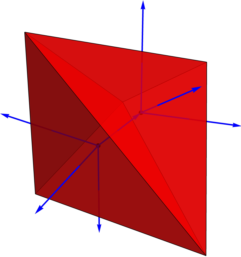
Figure 9: A simple discretization with two cells (in red) and a dual spin network (in blue). Here, the discretization is the simplest possible one: a simplicial complex, where the cells are 3-simplices (tetrahedrons) and their faces are 2-simplices (triangles). The edges are 1-simplices (line segments), and the vertices are, of course, 0-simplices (points). However, our formalism also allows the cells to be arbitrary convex polyhedra and the faces to be arbitrary convex polygons. From the figure, it should be clear that each of the two cells is dual to a node (located inside it), and each of the faces is dual to a link, with the face shared by the two cells dual to the link connecting the two nodes. This is further illustrated by Figure 10.

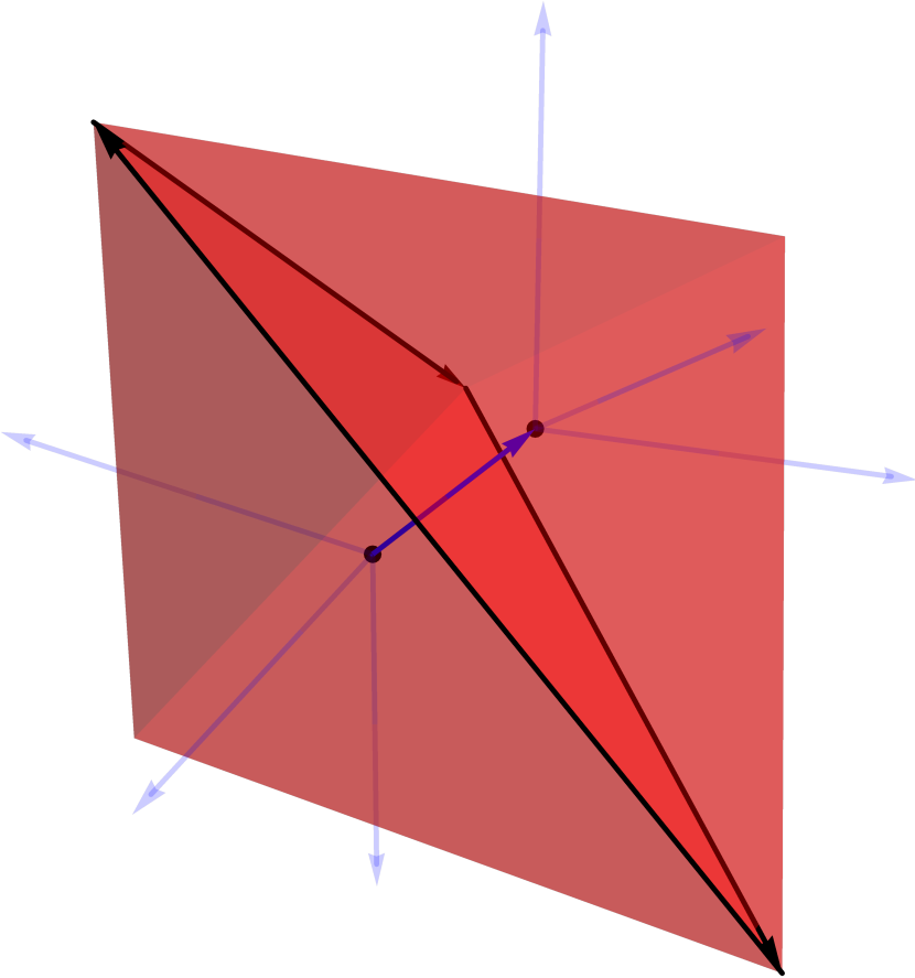
Figure 10: For clarity, we have highlighted the middle link, the two nodes it connects, the (triangular) face shared by the two cells, and the edges on the boundary on that face (which are, as illustrated, oriented) – and dimmed everything else.

In the 3+1-dimensional case, it would make sense to generalize the disks we defined in the 2+1-dimensional case to cylinders which surround the edges. This construction is left for future work; in this thesis, we will not worry about regularizing the singularities, and instead just use holonomies to probe the curvature and torsion in an indirect manner, as will be shown below.

14.2 Truncating the Geometry to the Edges

The connection and frame field inside each cell $c$ – that is, on the interior of the cell, but not on the edges and vertices – are taken to be

$$\mathbf{A}\bigl{|}_{c}=h_{c}^{-1}\mathrm{d}h_{c},\qquad\mathbf{e}\bigl{|}_{c}=h_{c}^{-1}\mathrm{d}\mathbf{x}_{c}h_{c}\quad\Longrightarrow\quad\mathbf{E}\bigl{|}_{c}=\frac{1}{2}\left[\mathbf{e},\mathbf{e}\right]\bigl{|}_{c}=h_{c}^{-1}\left[\mathrm{d}\mathbf{x}_{c},\mathrm{d}\mathbf{x}_{c}\right]h_{c},$$ (14.1)

in analogy with the 2+1D case. Since they correspond to

$$\mathbf{F}\equiv\mathrm{d}_{\mathbf{A}}\mathbf{A}=0,\qquad\mathbf{P}\equiv\mathrm{d}_{\mathbf{A}}\mathbf{e}=0,$$ (14.2)

they trivially solve all of the constraints:

$$\left[\mathbf{e},\mathbf{P}\right]=\left[\mathbf{e},\mathbf{F}\right]=\mathbf{e}\cdot\mathbf{F}-\frac{1}{2}\left(\frac{1}{\gamma}+\gamma\right)\mathbf{K}\cdot\mathbf{P}=0.$$ (14.3)

We also impose that $\mathbf{F}$ and $\mathbf{P}$ are non-zero only on the edges:

$$\mathbf{F}=\sum_{e}\mathbf{p}_{e}\delta\left(e\right),\qquad\mathbf{T}=\sum_{e}\mathbf{j}_{e}\delta\left(e\right),$$ (14.4)

where $\delta\left(e\right)$ is a 2-form delta function such that for any 1-form $f$

$$\int_{\Sigma}f\wedge\delta\left(e\right)=\int_{e}f,$$ (14.5)

as discussed in Chapter 13, and $\mathbf{p}_{e}$ and $\mathbf{j}_{e}$ are constant algebra elements encoding the curvature and torsion, respectively, on each edge. These distributional curvature and torsion describe a network of cosmic strings: 1-dimensional topological defects carrying curvature and torsion in an otherwise flat spacetime. The expressions (14.4) are derived from first principles in Chapter 13.

This construction describes a piecewise-flat-and-torsionless geometry; the cells are flat and torsionless, and the curvature and torsion are located only on the edges of the cells. We may interpret the 1-skeleton $\Gamma$, the set of all edges in the cellular decomposition $\Delta$, as a network of cosmic strings.

The reason for considering this particular geometry comes from the assumption that the geometry can only be probed by taking loops of holonomies along the spin network. Imagine a 3-dimensional slice $\Sigma$ with arbitrary geometry. We first embed a spin network $\Gamma^{*}$, which can be any graph, in $\Sigma$. Then we draw a dual graph, $\Gamma$, such that each edge of $\Gamma$ passes through exactly one loop of $\Gamma^{*}$. We take a holonomy along each of the loops of $\Gamma^{*}$, and encode the result on the edges of $\Gamma$. The resulting discrete geometry is exactly the one we described above, and it is completely equivalent to the continuous geometry with which we started, since the holonomies along the spin network cannot tell the difference between the continuous geometry and the discrete one.

In short, given a choice of a particular spin network, an arbitrary continuous geometry may be reduced to an equivalent discrete geometry, given by a network of cosmic strings, one for each loop of the spin network.

15 Discretizing the Symplectic Potential

15.1 First Step: From Continuous to Discrete Variables

We start with the symplectic potential obtained in (12.165),

$$\Theta=-\int_{\Sigma}\mathbf{E}\cdot\delta\mathbf{A}.$$ (15.1)

Using the identity

$$\delta\mathbf{A}\bigl{|}_{c}=h_{c}^{-1}\left(\mathrm{d}\boldsymbol{\Delta}h_{c}\right)h_{c},$$ (15.2)

the potential becomes

$$\Theta=-\sum_{c}\int_{c}\left[\mathrm{d}\mathbf{x}_{c},\mathrm{d}\mathbf{x}_{c}\right]\cdot\mathrm{d}\boldsymbol{\Delta}h_{c}.$$ (15.3)

To use Stokes’ theorem in the first integral, we note that

$$\left[\mathrm{d}\mathbf{x}_{c},\mathrm{d}\mathbf{x}_{c}\right]\cdot\mathrm{d}\boldsymbol{\Delta}h_{c}=\mathrm{d}\left(\left[\mathrm{d}\mathbf{x}_{c},\mathrm{d}\mathbf{x}_{c}\right]\cdot\boldsymbol{\Delta}h_{c}\right)=\mathrm{d}\left(\left[\mathbf{x}_{c},\mathrm{d}\mathbf{x}_{c}\right]\cdot\mathrm{d}\boldsymbol{\Delta}h_{c}\right),$$ (15.4)

hence we can write

$$\left[\mathrm{d}\mathbf{x}_{c},\mathrm{d}\mathbf{x}_{c}\right]\cdot\mathrm{d}\boldsymbol{\Delta}h_{c}=\left(1-\lambda\right)\mathrm{d}\left(\left[\mathrm{d}\mathbf{x}_{c},\mathrm{d}\mathbf{x}_{c}\right]\cdot\boldsymbol{\Delta}h_{c}\right)+\lambda\mathrm{d}\left(\left[\mathbf{x}_{c},\mathrm{d}\mathbf{x}_{c}\right]\cdot\mathrm{d}\boldsymbol{\Delta}h_{c}\right),$$ (15.5)

so

$$\Theta=-\sum_{c}\int_{\partial c}\left(\left(1-\lambda\right)\left[\mathrm{d}\mathbf{x}_{c},\mathrm{d}\mathbf{x}_{c}\right]\cdot\boldsymbol{\Delta}h_{c}+\lambda\left[\mathbf{x}_{c},\mathrm{d}\mathbf{x}_{c}\right]\cdot\mathrm{d}\boldsymbol{\Delta}h_{c}\right).$$ (15.6)

As in the 2+1D case, we have a family of polarizations corresponding to different values of $\lambda\in\left[0,1\right]$.

15.2 Second Step: From Cells to Sides

Next we decompose the boundary $\partial c$ of each cell $c=\left(s_{1},\ldots,s_{n}\right)$ into sides $s_{1},\ldots,s_{n}$. Each side $s=\left(cc^{\prime}\right)$ will have exactly two contributions, one from the cell $c$ and another, with opposite sign, from the cell $c^{\prime}$. We thus rewrite $\Theta$ as

$$\Theta=-\sum_{\left(cc^{\prime}\right)}\int_{\left(cc^{\prime}\right)}\left(I_{c^{\prime}}-I_{c}\right),$$ (15.7)

where

$$I_{c}\equiv\left(1-\lambda\right)\left[\mathrm{d}\mathbf{x}_{c},\mathrm{d}\mathbf{x}_{c}\right]\cdot\boldsymbol{\Delta}h_{c}+\lambda\left[\mathbf{x}_{c},\mathrm{d}\mathbf{x}_{c}\right]\cdot\mathrm{d}\boldsymbol{\Delta}h_{c}.$$ (15.8)

Now, in the 3+1D case we have the continuity conditions, derived in the same way as in Section 6.4:

$$h_{c^{\prime}}=h_{c^{\prime}c}h_{c},\qquad\mathbf{x}_{c^{\prime}}=h_{c^{\prime}c}(\mathbf{x}_{c}-\mathbf{x}_{c}^{c^{\prime}})h_{cc^{\prime}},$$ (15.9)

$$\boldsymbol{\Delta}h_{c^{\prime}}=\boldsymbol{\Delta}\left(h_{c^{\prime}c}h_{c}\right)=h_{c^{\prime}c}\left(\boldsymbol{\Delta}h_{c}-\boldsymbol{\Delta}h_{c}^{c^{\prime}}\right)h_{cc^{\prime}},$$ (15.10)

$$\mathrm{d}\boldsymbol{\Delta}h_{c^{\prime}}=h_{c^{\prime}c}\mathrm{d}\boldsymbol{\Delta}h_{c}h_{cc^{\prime}},$$ (15.11)

$$\mathrm{d}\mathbf{x}_{c^{\prime}}=\mathrm{d}\left(h_{c^{\prime}c}(\mathbf{x}_{c}-\mathbf{x}_{c}^{c^{\prime}})h_{cc^{\prime}}\right)=h_{c^{\prime}c}\mathrm{d}\mathbf{x}_{c}h_{cc^{\prime}},$$ (15.12)

where all of the conditions are valid only on the side $s=\left(cc^{\prime}\right)$. Using these conditions, we find that

$$I_{c^{\prime}} =\left(1-\lambda\right)\left[\mathrm{d}\mathbf{x}_{c^{\prime}},\mathrm{d}\mathbf{x}_{c^{\prime}}\right]\cdot\boldsymbol{\Delta}h_{c^{\prime}}+\lambda\left[\mathbf{x}_{c^{\prime}},\mathrm{d}\mathbf{x}_{c^{\prime}}\right]\cdot\mathrm{d}\boldsymbol{\Delta}h_{c^{\prime}}$$

$$=\left(1-\lambda\right)\left[\mathrm{d}\mathbf{x}_{c},\mathrm{d}\mathbf{x}_{c}\right]\cdot\left(\boldsymbol{\Delta}h_{c}-\boldsymbol{\Delta}h_{c}^{c^{\prime}}\right)+\lambda\left[\mathbf{x}_{c}-\mathbf{x}_{c}^{c^{\prime}},\mathrm{d}\mathbf{x}_{c}\right]\cdot\mathrm{d}\boldsymbol{\Delta}h_{c}.$$

Comparing with $I_{c}$, we see that many terms cancel, and we are left with

$$\Theta=\sum_{\left(cc^{\prime}\right)}\int_{\left(cc^{\prime}\right)}\left(\left(1-\lambda\right)\left[\mathrm{d}\mathbf{x}_{c},\mathrm{d}\mathbf{x}_{c}\right]\cdot\boldsymbol{\Delta}h_{c}^{c^{\prime}}+\lambda\left[\mathbf{x}_{c}^{c^{\prime}},\mathrm{d}\mathbf{x}_{c}\right]\cdot\mathrm{d}\boldsymbol{\Delta}h_{c}\right).$$ (15.13)

Since $\boldsymbol{\Delta}h_{c}^{c^{\prime}}$ and $\mathbf{x}_{c}^{c^{\prime}}$ are constant, we may rewrite this as

$$\Theta=\sum_{\left(cc^{\prime}\right)}\left(\left(1-\lambda\right)\boldsymbol{\Delta}h_{c}^{c^{\prime}}\cdot\int_{\left(cc^{\prime}\right)}\left[\mathrm{d}\mathbf{x}_{c},\mathrm{d}\mathbf{x}_{c}\right]+\lambda\mathbf{x}_{c}^{c^{\prime}}\cdot\int_{\left(cc^{\prime}\right)}\left[\mathrm{d}\mathbf{x}_{c},\mathrm{d}\boldsymbol{\Delta}h_{c}\right]\right).$$ (15.14)

Now, in order to use Stokes’ theorem again, we can write

$$\left[\mathrm{d}\mathbf{x}_{c},\mathrm{d}\mathbf{x}_{c}\right]=\mathrm{d}\left[\mathbf{x}_{c},\mathrm{d}\mathbf{x}_{c}\right],$$ (15.15)

and

$$\left[\mathrm{d}\mathbf{x}_{c},\mathrm{d}\boldsymbol{\Delta}h_{c}\right]=\mathrm{d}\left[\mathbf{x}_{c},\mathrm{d}\boldsymbol{\Delta}h_{c}\right]=-\mathrm{d}\left[\mathrm{d}\mathbf{x}_{c},\boldsymbol{\Delta}h_{c}\right],$$ (15.16)

which we write, defining an additional polarization parameter $\mu\in\left[0,1\right]$, as

$$\left[\mathrm{d}\mathbf{x}_{c},\mathrm{d}\boldsymbol{\Delta}h_{c}\right]=\left(1-\mu\right)\mathrm{d}\left[\mathbf{x}_{c},\mathrm{d}\boldsymbol{\Delta}h_{c}\right]-\mu\mathrm{d}\left[\mathrm{d}\mathbf{x}_{c},\boldsymbol{\Delta}h_{c}\right].$$ (15.17)

The symplectic potential now becomes

$$\Theta=\sum_{\left(cc^{\prime}\right)}\left(\left(1-\lambda\right)\boldsymbol{\Delta}h_{c}^{c^{\prime}}\cdot\int_{\partial\left(cc^{\prime}\right)}\left[\mathbf{x}_{c},\mathrm{d}\mathbf{x}_{c}\right]+\lambda\mathbf{x}_{c}^{c^{\prime}}\cdot\int_{\partial\left(cc^{\prime}\right)}\left(\left(1-\mu\right)\left[\mathbf{x}_{c},\mathrm{d}\boldsymbol{\Delta}h_{c}\right]-\mu\left[\mathrm{d}\mathbf{x}_{c},\boldsymbol{\Delta}h_{c}\right]\right)\right),$$ (15.18)

and it describes a two-parameter family of potentials for each value of $\lambda\in\left[0,1\right]$ and $\mu\in\left[0,1\right]$.

15.3 Third Step: From Sides to Edges

The boundary $\partial s$ of each side $s=\left(e_{1},\ldots,e_{n}\right)$ is composed of edges $e$. Conversely, each edge $e=\left(s_{1},\ldots,s_{N_{e}}\right)$ is part of the boundary of $N_{e}$ different sides, which we label in sequential order $s_{i}\equiv\left(c_{i}c_{i+1}\right)$ for $i\in\left\{1,\ldots,N_{e}\right\}$, with the convention that $c_{N_{e}+1}$ is the same as $c_{1}$ after encircling the edge $e$ once. Note that this sequence of sides is dual to a loop of links $s_{i}^{*}=\left(c_{i}c_{i+1}\right)^{*}$ around the edge $e$. Then we can rearrange the integrals as follows:

$$\sum_{\left(cc^{\prime}\right)}\int_{\partial\left(cc^{\prime}\right)}=\sum_{e}\int_{e}\sum_{i=1}^{N_{e}}.$$ (15.19)

The potential becomes

$$\Theta=\sum_{e}\int_{e}\sum_{i=1}^{N_{e}}I_{c_{i}c_{i+1}},$$ (15.20)

where

$$I_{c_{i}c_{i+1}}\equiv\left(1-\lambda\right)\boldsymbol{\Delta}h_{c_{i}}^{c_{i+1}}\cdot\left[\mathbf{x}_{c_{i}},\mathrm{d}\mathbf{x}_{c_{i}}\right]+\lambda\mathbf{x}_{c_{i}}^{c_{i+1}}\cdot\left(\left(1-\mu\right)\left[\mathbf{x}_{c_{i}},\mathrm{d}\boldsymbol{\Delta}h_{c_{i}}\right]-\mu\left[\mathrm{d}\mathbf{x}_{c_{i}},\boldsymbol{\Delta}h_{c_{i}}\right]\right).$$ (15.21)

We would like to perform a final integration using Stokes’ theorem. For this we again need to somehow cancel some elements, as we did before. However, since there are now $N_{e}$ different contributions, we cannot use the continuity conditions between each pair of adjacent cells, since in order to get cancellations, all terms must have the same base point (subscript).

One option is to choose a particular cell and trace everything back to that cell. However, this forces us to choose a specific cell for each edge. A more symmetric solution involves splitting each holonomy $h_{c_{i}c_{i+1}}$, which goes from from $c_{i}^{*}$ to $c_{i+1}^{*}$, into two holonomies – first going from $c_{i}^{*}$ to (some arbitrary point $e_{0}$ on) $e$ and then back to $c_{i+1}^{*}$, using the recipe given in Section 2.6:

$$h_{c_{i}c_{i+1}}=h_{c_{i}e}h_{ec_{i+1}},\qquad\mathbf{x}_{c_{i}}^{c_{i+1}}=\mathbf{x}_{c_{i}}^{e}\oplus\mathbf{x}_{e}^{c_{i+1}}=\mathbf{x}_{c_{i}}^{e}+h_{c_{i}e}\mathbf{x}_{e}^{c_{i+1}}h_{ec_{i}}=h_{c_{i}e}\left(\mathbf{x}_{e}^{c_{i+1}}-\mathbf{x}_{e}^{c_{i}}\right)h_{ec_{i}}.$$ (15.22)

From this we find that

$$\boldsymbol{\Delta}h_{c_{i}}^{c_{i+1}}=h_{c_{i}e}\left(\boldsymbol{\Delta}h_{e}^{c_{i+1}}-\boldsymbol{\Delta}h_{e}^{c_{i}}\right)h_{ec_{i}}.$$ (15.23)

Therefore

$$I_{c_{i}c_{i+1}} =\left(1-\lambda\right)h_{c_{i}e}\left(\boldsymbol{\Delta}h_{e}^{c_{i+1}}-\boldsymbol{\Delta}h_{e}^{c_{i}}\right)h_{ec_{i}}\cdot\left[\mathbf{x}_{c_{i}},\mathrm{d}\mathbf{x}_{c_{i}}\right]+$$

$$\qquad+\lambda h_{c_{i}e}\left(\mathbf{x}_{e}^{c_{i+1}}-\mathbf{x}_{e}^{c_{i}}\right)h_{ec_{i}}\cdot\left(\left(1-\mu\right)\left[\mathbf{x}_{c_{i}},\mathrm{d}\boldsymbol{\Delta}h_{c_{i}}\right]-\mu\left[\mathrm{d}\mathbf{x}_{c_{i}},\boldsymbol{\Delta}h_{c_{i}}\right]\right).$$

Furthermore, we have the usual continuity conditions between a cell $c_{i}$ and the edge $e$:

$$\mathbf{x}_{c_{i}}=h_{c_{i}e}\left(\mathbf{x}_{e}-\mathbf{x}_{e}^{c_{i}}\right)h_{ec_{i}},\qquad\mathrm{d}\mathbf{x}_{c_{i}}=h_{c_{i}e}\mathrm{d}\mathbf{x}_{e}h_{ec_{i}},$$ (15.24)

$$h_{c_{i}}=h_{c_{i}e}h_{e},\qquad\boldsymbol{\Delta}h_{c_{i}}=h_{c_{i}e}\left(\boldsymbol{\Delta}h_{e}-\boldsymbol{\Delta}h_{e}^{c_{i}}\right)h_{ec_{i}},\qquad\mathrm{d}\boldsymbol{\Delta}h_{c_{i}}=h_{c_{i}e}\mathrm{d}\boldsymbol{\Delta}h_{e}h_{ec_{i}}.$$ (15.25)

If we had a cylinder around the edge $e$, then these conditions would have been valid on the boundary between the cylinder and the cell. However, in the case we are considering here, the cylinder has zero radius, so these conditions are instead valid on the edge $e$ itself.

Plugging in, we get

$$I_{c_{i}c_{i+1}} =\left(1-\lambda\right)\left(\boldsymbol{\Delta}h_{e}^{c_{i+1}}-\boldsymbol{\Delta}h_{e}^{c_{i}}\right)\cdot\left[\mathbf{x}_{e}-\mathbf{x}_{e}^{c_{i}},\mathrm{d}\mathbf{x}_{e}\right]+$$

$$\qquad+\lambda\left(\mathbf{x}_{e}^{c_{i+1}}-\mathbf{x}_{e}^{c_{i}}\right)\cdot\left(\left(1-\mu\right)\left[\mathbf{x}_{e}-\mathbf{x}_{e}^{c_{i}},\mathrm{d}\boldsymbol{\Delta}h_{e}\right]-\mu\left[\mathrm{d}\mathbf{x}_{e},\boldsymbol{\Delta}h_{e}-\boldsymbol{\Delta}h_{e}^{c_{i}}\right]\right).$$

Now we sum over all the terms, and take anything that does not depend on $i$ out of the sum and anything that is constant out of the integral. We get

$$\Theta=\sum_{e}\left(\Theta_{e}+\sum_{i=1}^{N_{e}}\Theta_{e}^{c_{i}c_{i+1}}\right),$$ (15.26)

where

$$\Theta_{e} \equiv\left(1-\lambda\right)\int_{e}\left[\mathbf{x}_{e},\mathrm{d}\mathbf{x}_{e}\right]\cdot\sum_{i=1}^{N_{e}}\left(\boldsymbol{\Delta}h_{e}^{c_{i+1}}-\boldsymbol{\Delta}h_{e}^{c_{i}}\right)+$$

$$\qquad+\lambda\left(\left(1-\mu\right)\int_{e}\left[\mathbf{x}_{e},\mathrm{d}\boldsymbol{\Delta}h_{e}\right]-\mu\int_{e}\left[\mathrm{d}\mathbf{x}_{e},\boldsymbol{\Delta}h_{e}\right]\right)\cdot\sum_{i=1}^{N_{e}}\left(\mathbf{x}_{e}^{c_{i+1}}-\mathbf{x}_{e}^{c_{i}}\right),$$

$$\Theta_{e}^{c_{i}c_{i+1}} \equiv-\left(1-\lambda\right)\left[\mathbf{x}_{e}^{c_{i}},\int_{e}\mathrm{d}\mathbf{x}_{e}\right]\cdot\left(\boldsymbol{\Delta}h_{e}^{c_{i+1}}-\boldsymbol{\Delta}h_{e}^{c_{i}}\right)+$$

$$\qquad-\lambda\left(\mathbf{x}_{e}^{c_{i+1}}-\mathbf{x}_{e}^{c_{i}}\right)\cdot\left(\left(1-\mu\right)\left[\mathbf{x}_{e}^{c_{i}},\int_{e}\mathrm{d}\boldsymbol{\Delta}h_{e}\right]-\mu\left[\int_{e}\mathrm{d}\mathbf{x}_{e},\boldsymbol{\Delta}h_{e}^{c_{i}}\right]\right).$$

Note that $\Theta_{e}$ exists uniquely for each edge, while $\Theta_{e}^{c_{i}c_{i+1}}$ exists uniquely for each combination of edge $e$ and side $\left(c_{i}c_{i+1}\right)$.

15.4 The Edge Potential

In $\Theta_{e}$, we notice that both sums are telescoping – each term cancels out one other term, and we are left with only the first and last term:

$$\sum_{i=1}^{N_{e}}\left(\boldsymbol{\Delta}h_{e}^{c_{i+1}}-\boldsymbol{\Delta}h_{e}^{c_{i}}\right) =\left(\boldsymbol{\Delta}h_{e}^{c_{2}}-\boldsymbol{\Delta}h_{e}^{c_{1}}\right)+\left(\boldsymbol{\Delta}h_{e}^{c_{3}}-\boldsymbol{\Delta}h_{e}^{c_{2}}\right)+\cdots+\left(\boldsymbol{\Delta}h_{e}^{c_{N_{e}+1}}-\boldsymbol{\Delta}h_{e}^{c_{N_{e}}}\right)$$

$$=\boldsymbol{\Delta}h_{e}^{c_{N_{e}+1}}-\boldsymbol{\Delta}h_{e}^{c_{1}},$$

$$\sum_{i=1}^{N_{e}}\left(\mathbf{x}_{e}^{c_{i+1}}-\mathbf{x}_{e}^{c_{i}}\right) =\left(\mathbf{x}_{e}^{c_{2}}-\mathbf{x}_{e}^{c_{1}}\right)+\left(\mathbf{x}_{e}^{c_{3}}-\mathbf{x}_{e}^{c_{2}}\right)+\cdots+\left(\mathbf{x}_{e}^{c_{N_{e}+1}}-\mathbf{x}_{e}^{c_{N_{e}}}\right)$$

$$=\mathbf{x}_{e}^{c_{N_{e}+1}}-\mathbf{x}_{e}^{c_{1}}.$$

Now, $c_{N_{e}+1}$ is the same as $c_{1}$ after encircling $e$ once. So, if the geometry is completely flat and torsionless, we can just say that $\Theta_{e}$ vanishes. However, if the edge carries curvature and/or torsion, then after winding around the edge once, the rotational and translational holonomies should detect them. This is illustrated in Figure 11. We choose to label this as follows:

$$\boldsymbol{\Delta}h_{e}^{c_{N_{e}+1}}-\boldsymbol{\Delta}h_{e}^{c_{1}}\equiv\delta\mathbf{M}_{e},\qquad\mathbf{x}_{e}^{c_{N_{e}+1}}-\mathbf{x}_{e}^{c_{1}}\equiv\SS_{e}.$$ (15.27)

The values of $\mathbf{M}_{e}$ and $\SS_{e}$ in (15.27) are directly related to the values of $\mathbf{p}_{e}$ and $\mathbf{j}_{e}$ in (14.4), which determine the momentum and angular momentum of the string that lies on the edge $e$. We may interpret (15.27) in two ways. Either we first find $\mathbf{M}_{e}$ and $\SS_{e}$ by calculating the difference of holonomies, as defined in (15.27), and then define $\mathbf{p}_{e}$ and $\mathbf{j}_{e}$ in (14.4) as functions of these quantities – or, conversely, we start with strings that have well-defined momentum and angular momentum $\mathbf{p}_{e}$ and $\mathbf{j}_{e}$, and then define $\mathbf{M}_{e}$ and $\SS_{e}$ as appropriate functions of $\mathbf{p}_{e}$ and $\mathbf{j}_{e}$.

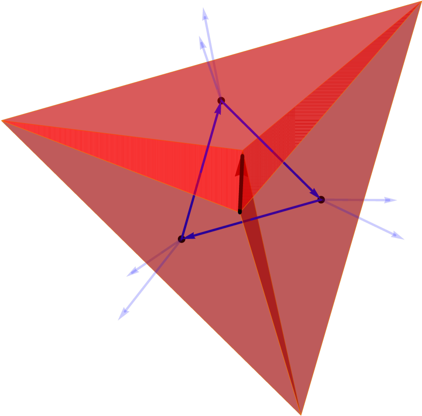
Figure 11: Three cells (tetrahedrons, in red) dual to three nodes (in black). The cells share three faces (highlighted) which are dual to three oriented links (blue arrows) connecting the nodes. The three links form a loop, which goes around the single edge shared by all three cells (the thick black arrow in the middle). By taking a holonomy around the loop $\left(c_{1}c_{2}c_{3}c_{1}\right)$, we can detect the curvature and torsion encoded in the middle edge.

Unfortunately, aside from this simplification, it does not seem possible to simplify $\Theta_{e}$ any further, since there is no obvious way to write the integrands as exact 1-forms. The only thing left for us to do, therefore, is to call the integrals by names:

$$\mathbf{X}_{e}\equiv\int_{e}\left[\mathbf{x}_{e},\mathrm{d}\mathbf{x}_{e}\right],\qquad\boldsymbol{\Delta}H_{e}^{1}\equiv\int_{e}\left[\mathbf{x}_{e},\mathrm{d}\boldsymbol{\Delta}h_{e}\right],\qquad\boldsymbol{\Delta}H_{e}^{2}\equiv\int_{e}\left[\mathrm{d}\mathbf{x}_{e},\boldsymbol{\Delta}h_{e}\right],$$ (15.28)

and write:

$$\Theta_{e}=\left(1-\lambda\right)\mathbf{X}_{e}\cdot\delta\mathbf{M}_{e}+\lambda\SS_{e}\cdot\left(\left(1-\mu\right)\boldsymbol{\Delta}H_{e}^{1}-\mu\boldsymbol{\Delta}H_{e}^{2}\right).$$ (15.29)

In fact, since both $H_{e}^{1}$ and $H_{e}^{2}$ are conjugate to the same variable $\SS_{e}$, we might as well collect them into a single variable:

$$\boldsymbol{\Delta}H_{e}\equiv\left(1-\mu\right)\boldsymbol{\Delta}H_{e}^{1}-\mu\boldsymbol{\Delta}H_{e}^{2},$$ (15.30)

so that the choice of parameter $\mu\in\left[0,1\right]$ simply chooses how much of $H_{e}^{1}$ compared to $H_{e}^{2}$ is used this variable. We obtain:

$$\Theta_{e}=\left(1-\lambda\right)\mathbf{X}_{e}\cdot\delta\mathbf{M}_{e}+\lambda\SS_{e}\cdot\boldsymbol{\Delta}H_{e}.$$ (15.31)

This term is remarkably similar to the vertex potential we found in the second line of (11.33) in the analysis of corner modes in 2+1D. Indeed, the derivation here is very much analogous to the derivation of Chapter 11. This term encodes the dynamics of the curvature and torsion on each edge $e$. In fact, if we perform a change of variables:

$$\left(1-\lambda\right)\mathbf{X}_{e}\mapsto\mathbf{X}_{e},\qquad\lambda\SS_{e}\mapsto-\left(\SS_{e}+\left[\mathbf{M}_{e},\mathbf{X}_{e}\right]\right),$$ (15.32)

we obtain precisely the same term that we obtained in (8.35):

$$\Theta_{e}=\mathbf{X}_{e}\cdot\delta\mathbf{M}_{e}-\left(\SS_{e}+\left[\mathbf{M}_{e},\mathbf{X}_{e}\right]\right)\cdot\boldsymbol{\Delta}H_{e}.$$ (15.33)

15.5 The Link Potential

The term $\Theta_{e}^{c_{i}c_{i+1}}$, defined at the end of Section 15.3, is easily integrable. Since we don’t need the telescoping sum anymore, we can simplify this term by returning to the original variables:

$$\mathbf{x}_{e}^{c_{i+1}}-\mathbf{x}_{e}^{c_{i}}=h_{ec_{i}}\mathbf{x}_{c_{i}}^{c_{i+1}}h_{c_{i}e},\qquad\boldsymbol{\Delta}h_{e}^{c_{i+1}}-\boldsymbol{\Delta}h_{e}^{c_{i}}=h_{ec_{i}}\boldsymbol{\Delta}h_{c_{i}}^{c_{i+1}}h_{c_{i}e},$$ (15.34)

so it becomes

$$\Theta_{e}^{c_{i}c_{i+1}} =-\left(1-\lambda\right)\left[\mathbf{x}_{e}^{c_{i}},\int_{e}\mathrm{d}\mathbf{x}_{e}\right]\cdot h_{ec_{i}}\boldsymbol{\Delta}h_{c_{i}}^{c_{i+1}}h_{c_{i}e}+$$

$$\qquad-\lambda h_{ec_{i}}\mathbf{x}_{c_{i}}^{c_{i+1}}h_{c_{i}e}\cdot\left(\left(1-\mu\right)\left[\mathbf{x}_{e}^{c_{i}},\int_{e}\mathrm{d}\boldsymbol{\Delta}h_{e}\right]-\mu\left[\int_{e}\mathrm{d}\mathbf{x}_{e},\boldsymbol{\Delta}h_{e}^{c_{i}}\right]\right).$$

We also have the usual inversion relations (see Section 2.7)

$$h_{c_{i}e}\mathbf{x}_{e}^{c_{i}}h_{ec_{i}}=-\mathbf{x}_{c_{i}}^{e},\qquad,h_{c_{i}e}\boldsymbol{\Delta}h_{e}^{c_{i}}h_{ec_{i}}=-\boldsymbol{\Delta}h_{c_{i}}^{e},$$ (15.35)

so we can further simplify to:

$$\Theta_{e}^{c_{i}c_{i+1}} =\left(1-\lambda\right)\left[\mathbf{x}_{c_{i}}^{e},h_{c_{i}e}\left(\int_{e}\mathrm{d}\mathbf{x}_{e}\right)h_{ec_{i}}\right]\cdot\boldsymbol{\Delta}h_{c_{i}}^{c_{i+1}}+$$

$$\qquad+\lambda\mathbf{x}_{c_{i}}^{c_{i+1}}\cdot\left(\left(1-\mu\right)\left[\mathbf{x}_{c_{i}}^{e},h_{c_{i}e}\left(\int_{e}\mathrm{d}\boldsymbol{\Delta}h_{e}\right)h_{ec_{i}}\right]+\mu\left[h_{c_{i}e}\left(\int_{e}\mathrm{d}\mathbf{x}_{e}\right)h_{ec_{i}},\boldsymbol{\Delta}h_{c_{i}}^{e}\right]\right).$$

Next, we assume that the edge $e$ starts at the vertex $v$ and ends at the vertex $v^{\prime}$, i.e. $e=\left(vv^{\prime}\right)$. Then we can evaluate the integrals explicitly:

$$\int_{e}\mathrm{d}\boldsymbol{\Delta}h_{e}=\boldsymbol{\Delta}h_{e}\left(v^{\prime}\right)-\boldsymbol{\Delta}h_{e}\left(v\right),\qquad\int_{e}\mathrm{d}\mathbf{x}_{e}=\mathbf{x}_{e}\left(v^{\prime}\right)-\mathbf{x}_{e}\left(v\right).$$ (15.36)

Now, let $h_{vv^{\prime}}$ and $\mathbf{x}_{v}^{v^{\prime}}$ be the rotational and translational holonomies along the edge $e$, that is, from $v$ to $v^{\prime}$. Then we can split them so that they also pass through a point $e_{0}$ on the edge $e$, as follows:

$$h_{vv^{\prime}}=h_{ve}h_{ev^{\prime}}\quad\Longrightarrow\quad\boldsymbol{\Delta}h_{v}^{v^{\prime}}=h_{ve}\left(\boldsymbol{\Delta}h_{e}^{v^{\prime}}-\boldsymbol{\Delta}h_{e}^{v}\right)h_{ev},$$ (15.37)

$$\mathbf{x}_{v}^{v^{\prime}}=\mathbf{x}_{v}^{e}\oplus\mathbf{x}_{e}^{v^{\prime}}=h_{ve}\left(\mathbf{x}_{e}^{v^{\prime}}-\mathbf{x}_{e}^{v}\right)h_{ev},$$ (15.38)

in analogy with (11.37) and (11.38). Given that $h_{e}\left(v\right)=h_{ev}$ and $\mathbf{x}_{e}\left(v\right)=\mathbf{x}_{e}^{v}$, the integrals may now be written as

$$\int_{e}\mathrm{d}\boldsymbol{\Delta}h_{e}=h_{ev}\boldsymbol{\Delta}h_{v}^{v^{\prime}}h_{ve},\qquad\int_{e}\mathrm{d}\mathbf{x}_{e}=h_{ev}\mathbf{x}_{v}^{v^{\prime}}h_{ve}.$$ (15.39)

Moreover, since $h_{c_{i}e}h_{ev}=h_{c_{i}v}$, we have

$$h_{c_{i}e}\left(\int_{e}\mathrm{d}\boldsymbol{\Delta}h_{e}\right)h_{ec_{i}}=h_{c_{i}e}\left(h_{ev}\boldsymbol{\Delta}h_{v}^{v^{\prime}}h_{ve}\right)h_{ec_{i}}=h_{c_{i}v}\boldsymbol{\Delta}h_{v}^{v^{\prime}}h_{vc_{i}},$$ (15.40)

$$h_{c_{i}e}\left(\int_{e}\mathrm{d}\mathbf{x}_{e}\right)h_{ec_{i}}=h_{c_{i}e}\left(h_{ev}\mathbf{x}_{v}^{v^{\prime}}h_{ve}\right)h_{ec_{i}}=h_{c_{i}v}\mathbf{x}_{v}^{v^{\prime}}h_{vc_{i}}.$$ (15.41)

With this, we may simplify $\Theta_{e}^{c_{i}c_{i+1}}$ to

$$\Theta_{e}^{c_{i}c_{i+1}} =\left(1-\lambda\right)\left[\mathbf{x}_{c_{i}}^{e},h_{c_{i}v}\mathbf{x}_{v}^{v^{\prime}}h_{vc_{i}}\right]\cdot\boldsymbol{\Delta}h_{c_{i}}^{c_{i+1}}+$$

$$\qquad+\lambda\mathbf{x}_{c_{i}}^{c_{i+1}}\cdot\left(\left(1-\mu\right)\left[\mathbf{x}_{c_{i}}^{e},h_{c_{i}v}\boldsymbol{\Delta}h_{v}^{v^{\prime}}h_{vc_{i}}\right]+\mu\left[h_{c_{i}v}\mathbf{x}_{v}^{v^{\prime}}h_{vc_{i}},\boldsymbol{\Delta}h_{c_{i}}^{e}\right]\right).$$

15.6 Holonomies and Fluxes

Finally, in order to relate this to the spin network phase space, as we did in the 2+1D case, we need to identify holonomies and fluxes. From the 2+1D case, we know that the fluxes are in fact also holonomies – but they are translational, not rotational, holonomies. $h_{c_{i}c_{i+1}}$ is by definition the rotational holonomy on the link $\left(c_{i}c_{i+1}\right)^{*}$, and $\mathbf{x}_{c_{i}}^{c_{i+1}}$ is is by definition the translational holonomy on the link $\left(c_{i}c_{i+1}\right)^{*}$, so it’s natural to simply define

$$H_{c_{i}c_{i+1}}\equiv h_{c_{i}c_{i+1}},\qquad\mathbf{X}_{c_{i}}^{c_{i+1}}\equiv\mathbf{x}_{c_{i}}^{c_{i+1}}.$$ (15.42)

We should also define holonomies and fluxes on the sides dual to the links. By inspection, the flux on the side $\left(c_{i}c_{i+1}\right)$ must be

$$\tilde{\mathbf{X}}_{c_{i}}^{c_{i+1}}\equiv\left[\mathbf{x}_{c_{i}}^{v},h_{c_{i}v}\mathbf{x}_{v}^{v^{\prime}}h_{vc_{i}}\right].$$ (15.43)

Note that this expression depends only on the source cell $c_{i}$ and not on the target cell $c_{i+1}$, just as the analogous flux in the 2+1D case only depended on the source cell. This is an artifact of using the continuity conditions to write everything in terms of the source cell in order to make the expression integrable (and this is why we symmetrized the potential in Chapter (11) – the same can be done here, of course). The first term in the commutator is $\mathbf{x}_{c_{i}}^{v}$, the translational holonomy from the node $c_{i}^{*}$ to the vertex $v$, the starting point of $e$. The second term contains $\mathbf{x}_{v}^{v^{\prime}}$, the translational holonomy along the edge $e$.

As for holonomies on the sides – again, since we initially had two ways to integrate, we also have two different ways to define holonomies. However, as above, since both holonomies are conjugate to the same flux, $\mathbf{X}_{c_{i}}^{c_{i+1}}$, there is really no reason to differentiate them. Therefore we just define implicitly:

$$\boldsymbol{\Delta}\tilde{H}_{c_{i}}^{c_{i+1}}\equiv\left(1-\mu\right)\left[\mathbf{x}_{c_{i}}^{v},h_{c_{i}v}\boldsymbol{\Delta}h_{v}^{v^{\prime}}h_{vc_{i}}\right]+\mu\left[h_{c_{i}v}\mathbf{x}_{v}^{v^{\prime}}h_{vc_{i}},\boldsymbol{\Delta}h_{c_{i}}^{v}\right],$$ (15.44)

and the choice of parameter $\mu\in\left[0,1\right]$ simply determines how much of this holonomy comes from each polarization. We finally get:

$$\Theta_{e}^{c_{i}c_{i+1}}=\left(1-\lambda\right)\tilde{\mathbf{X}}_{c_{i}}^{c_{i+1}}\cdot\boldsymbol{\Delta}H_{c_{i}}^{c_{i+1}}+\lambda\mathbf{X}_{c_{i}}^{c_{i+1}}\cdot\boldsymbol{\Delta}\tilde{H}_{c_{i}}^{c_{i+1}}.$$ (15.45)

This is exactly the same term we obtained in the 2+1D case, (11.44)! It represents a holonomy-flux phase space on each link. For $\lambda=0$ the holonomies are on links and the fluxes are on their dual sides, while for the dual polarization $\lambda=1$ the fluxes are on the links and the holonomies are on the sides, in analogy with the two polarization we found in the 2+1D case.

15.7 Summary

We have obtained the following discrete symplectic potential:

$$\Theta=\sum_{e}\left(\left(1-\lambda\right)\mathbf{X}_{e}\cdot\delta\mathbf{M}_{e}+\lambda\SS_{e}\cdot\boldsymbol{\Delta}H_{e}+\sum_{i=1}^{N_{e}}\left(\left(1-\lambda\right)\tilde{\mathbf{X}}_{c_{i}}^{c_{i+1}}\cdot\boldsymbol{\Delta}H_{c_{i}}^{c_{i+1}}+\lambda\mathbf{X}_{c_{i}}^{c_{i+1}}\cdot\boldsymbol{\Delta}\tilde{H}_{c_{i}}^{c_{i+1}}\right)\right),$$ (15.46)

where for each edge $e$:

• $\left\{c_{1},\ldots,c_{N_{e}}\right\}$ are the $N_{e}$ cells around the edge,

• $\mathbf{X}_{e}\equiv\int_{e}\left[\mathbf{x}_{e},\mathrm{d}\mathbf{x}_{e}\right]$ is the “edge flux”,

• $\mathbf{M}_{e}$, defined implicitly by $\delta\mathbf{M}_{e}\equiv\boldsymbol{\Delta}h_{e}^{c_{N_{e}+1}}-\boldsymbol{\Delta}h_{e}^{c_{1}}$, represents the curvature on the edge,

• $\boldsymbol{\Delta}H_{e}\equiv\int_{e}\left(\left(1-\mu\right)\left[\mathbf{x}_{e},\mathrm{d}\boldsymbol{\Delta}h_{e}\right]-\mu\left[\mathrm{d}\mathbf{x}_{e},\boldsymbol{\Delta}h_{e}\right]\right)$ is the “edge holonomy”,

• $\SS_{e}\equiv\mathbf{x}_{e}^{c_{N_{e}+1}}-\mathbf{x}_{e}^{c_{1}}$ represents the torsion on the edge,

• $\tilde{\mathbf{X}}_{c_{i}}^{c_{i+1}}\equiv\left[\mathbf{x}_{c_{i}}^{v},h_{c_{i}v}\mathbf{x}_{v}^{v^{\prime}}h_{vc_{i}}\right]$ is the flux on the side $\left(c_{i}c_{i+1}\right)$ shared by the cells $c_{i}$ and $c_{i+1}$,

• $H_{c_{i}c_{i+1}}\equiv h_{c_{i}c_{i+1}}$ is the holonomy on the link $\left(c_{i}c_{i+1}\right)^{*}$ dual to the side $\left(c_{i}c_{i+1}\right)$,

• $\mathbf{X}_{c_{i}}^{c_{i+1}}\equiv\mathbf{x}_{c_{i}}^{c_{i+1}}$ is the flux on the link $\left(c_{i}c_{i+1}\right)^{*}$,

• $\tilde{H}_{c_{i}}^{c_{i+1}}$, defined implicitly by $\boldsymbol{\Delta}\tilde{H}_{c_{i}}^{c_{i+1}}\equiv\left(1-\mu\right)\left[\mathbf{x}_{c_{i}}^{v},h_{c_{i}v}\boldsymbol{\Delta}h_{v}^{v^{\prime}}h_{vc_{i}}\right]+\mu\left[h_{c_{i}v}\mathbf{x}_{v}^{v^{\prime}}h_{vc_{i}},\boldsymbol{\Delta}h_{c_{i}}^{v}\right]$, is the holonomy on the side $\left(c_{i}c_{i+1}\right)$.

We interpret this as the phase space of a spin network $\Gamma^{*}$ coupled to a network of cosmic strings $\Gamma$, with mass and spin related to the curvature and torsion.

16 Conclusions

16.1 Summary of Our Results

In this thesis, we performed a rigorous piecewise-flat-and-torsionless discretization of classical general relativity in the first-order formulation, in both 2+1 and 3+1 dimensions, carefully keeping track of curvature and torsion via holonomies. We showed that the resulting phase space is precisely that of spin networks, the quantum states of discrete spacetime in loop quantum gravity, with additional degrees of freedom called edge modes, which result from the discretization itself and possess their own unique symmetries.

The main contributions of this work are as follows.

1. It establishes, for the first time, a rigorous proof of the equivalence between spin networks and piecewise-flat geometries with curvature and torsion degrees of freedom.

In the 2+1-dimensional case, each node of the spin network is dual to a 2-dimensional cell, and each link connecting two nodes is dual to the edge shared by the two corresponding cells. A loop of links (or a face) is dual to a vertex of the cellular decomposition. These vertices are the locations where point particles reside, and by examining the value of the holonomies along the loop dual to a vertex, we learn about the curvature and torsion induced by the particle at the vertex by virtue of the Einstein equation.

In the 3+1-dimensional case, the situation is quite similar. Each node of the spin network is dual to a 3-dimensional cell, and each link connecting two nodes is dual to the side shared by the two corresponding cells. A loop of links (or a face) is dual to an edge of the cellular decomposition. These edges are the locations where strings reside, and by examining the value of the holonomies along the loop dual to an edge, we learn about the curvature and torsion induced by the string at the edge by virtue of the Einstein equation.

Equivalently, if we assume that the only way to detect curvature and torsion is by looking at appropriate holonomies on the loops of the spin networks, then we may interpret our result as taking some arbitrary continuous geometry, not necessarily generated by particles or strings, truncating it, and encoding it on the vertices in 2+1D or edges in 3+1D. The holonomies cannot tell the difference between a continuous geometry and a singular geometry; they can only tell us about the total curvature and torsion inside the loop.

As the spin networks are the quantum states of space and geometry is loop quantum gravity, our results illustrate a precise way in which these states can be assigned classical spatial geometries.

2. It demonstrates that careful consideration of edge modes is crucial both for the purpose of this proof and for future work in the field of loop quantum gravity.

Indeed, in Chapter 10 we analyzed the symmetries generated by the constraints and found that the entire symplectic form, not just the spin network terms but also the edge mode (or particle) term – which depends on the extra degrees of freedom $h_{v}\left(v\right)$ and $\mathbf{x}_{v}\left(v\right)$ and the curvature and torsion encoded in the variables $\mathbf{M}_{v}$ and $\SS_{v}$ – is invariant under this transformation.

Furthermore, in Section 8.4 we saw that the edge mode term transforms in a well-defined way under both right translations, corresponding to gauge transformations, and left translations, corresponding to an additional symmetry which did not exist in the continuous theory.

One could choose a particular gauge where the edge modes are “frozen”, that is, $h_{v}\left(v\right)=1$ and $\mathbf{x}_{v}\left(v\right)=0$. In this case, the entire particle term vanishes (in the limit where the disks are shrunk, $v_{0}\rightarrow v$). Freezing the edge modes makes exactly as much sense as any other gauge-fixing: it is convenient, but completely masks an important symmetry of our theory.

3. It set the stage for collaboration between the loop quantum gravity community and theoretical physicists working on edge modes from other perspectives, such as quantum electrodynamics, non-abelian gauge theories, and classical gravity.

This is especially important because loop quantum gravity has always been considered somewhat of a “fringe” theory. The study of edge modes has become increasingly popular in recent years among physicists who work on more “mainstream” theories, and interaction between the loop quantum gravity community and the physicists working on edge modes would no doubt be mutually beneficial for both communities.

4. It further developed the idea, introduced in [17] and later expanded in [58], that spin networks have a dual description related to teleparallel gravity, where gravity is encoded in torsion instead of curvature degrees of freedom.

In fact, we found a whole spectrum of theories for $\lambda\in\left[0,1\right]$, with the cases $\lambda=0$ (usual loop gravity), $\lambda=1$ (dual/teleparallel loop gravity), and possibly $\lambda=1/2$ (Chern-Simons theory) being of particular importance. We also analyzed the discrete constraints in detail in both polarizations. Importantly, we have discovered that this duality exists in both 2+1 and 3+1 dimensions, although we did not study it in detail in the latter case. The existence of this dual formulation of loop gravity may open up new avenues of research that have so far been unexplored, and new ways to tackle long-standing open problems in loop quantum gravity.

16.2 Future Plans

In this thesis we presented a very detailed analysis of the 2+1-dimensional toy model, which is, of course, simpler than the realistic 3+1-dimensional case. This analysis was performed with the philosophy that the 2+1D toy model can provide deep insights about the 3+1D theory.

Indeed, as we have seen in Parts III and IV, many structures from the 2+1D case, such as the cellular decomposition and its relation to the spin network, the rotational and translational holonomies and their properties, and the singular matter sources, can be readily generalized to the 3+1D with minimal modifications. Thus, the results of Parts I and II should be readily generalizable as well. As we have seen, we indeed obtain the same symplectic potential in both cases, which is not surprising – since we used the same structures in both.

However, the 3+1-dimensional case presents many challenges which would require much more work, far beyond the scope of this thesis, to overcome. Here we present some suggestions for possible research directions in 3+1D. Note that there are also many things one could explore in the 2+1D case, but we choose to focus on 3+1D since it is the physically relevant case. Of course, in many cases it would be beneficial to try introducing new structures (e.g. a cosmological constant) in the 2+1D case first, since the lessons learned from the toy theory may then be employed in the realistic theory – as we, indeed, did in this thesis.

1. Proper treatment of the singularities

In the 2+1D case, we carefully treated the 0-dimensional singularities, the point particles, by regularizing them with disks. This introduced many complications, but also ensured that our results were completely rigorous. In the 3+1D case, we skipped this crucial part, and instead jumped right to the end by assuming the results we had in 2+1D apply to the 3+1D case as well.

It would be instructive to repeat this in 3+1D and carefully treat the 1-dimensional singularities, the cosmic strings, by regularizing them with cylinders. Of course, this calculation will be much more involved than the one we did in 2+1D, as we now have to worry not only about the boundary of the disk but about the various boundaries of the cylinder. In particular, we must also regularize the vertices by spheres such that the top and bottom of each cylinder start on the surface of a sphere; this is further necessary in order to understand what happens at the points where several strings meet.

In attempts to perform this calculation, we encountered many mathematical and conceptual difficulties, which proved to be impossible to overcome within the scope of this thesis. Therefore, we leave it to future work.

2. Proper treatment of the edge modes

In the 2+1D case we analyzed the edge modes in detail, in particular by studying their role in the symplectic potential in both the continuous and discrete cases. However, in the 3+1D case we again skipped this and instead assumed our results from 2+1D still hold. In future work, we plan to perform a rigorous study of the edge modes in 3+1D, including their role in the symplectic potential and the new symmetries they generate.

3. Introducing a cosmological constant

In this thesis, we greatly simplified the calculation in 3+1 dimensions by imposing that the geometry inside the cells is flat, mimicking the 2+1-dimensional case. A more complicated case, but still probably doable within our framework, is incorporating a cosmological constant, which will then impose that the cells are homogeneously curved rather than flat. In this case, it would be instructive to perform the calculation in the 2+1D toy model first, and then generalize it to 3+1D.

4. Including point particles

Cosmic strings in 3+1D have a very similar mathematical structure to point particles in 2+1D (compare Chapters 5 and 13). For this reason, we used string-like defects as our sources of curvature and torsion in 3+1D, which then allowed us to generalize our results from 2+1D in a straightforward way. An important, but extremely complicated, modification would be to allow point particles in 3+1D as well.

More precisely, in 2+1D, we added sources for the curvature and torsion constraints, which are 2-forms. This is equivalent to adding matter sources on the right-hand side of the Einstein equation. Since these distributional sources are 2-form delta functions on a 2-dimensional spatial slice, they pick out 0-dimensional points, which we interpreted as a particle-like defects.

In 3+1D, we again added sources for the curvature and torsion, which in this case are not constraints, but rather imposed by hand to vanish. Since these distributional sources are 2-form delta functions on a 3-dimensional spatial slice, they pick out 1-dimensional strings. What we should actually do is add sources for the three constraints – Gauss, vector, and scalar – which are 3-forms. The 3-form delta functions will then pick out 0-dimensional points.

However, doing this would introduce several difficulties, both mathematical and conceptual. Perhaps the most serious problem would be that in 3 dimensions, once cannot place a vertex inside a loop. Indeed, in 2 dimensions, a loop encircling a vertex cannot be shrunk to a point, as it would have to pass through the vertex. Similarly, in 3 dimensions, a loop encircling an edge cannot be shrunk to a point without passing through the edge. Therefore, in these cases it makes sense to say that the vertex or edge is inside the loop.

However, in 3 dimensions there is no well-defined way in which a vertex can be said to be inside a loop; any loop can always be shrunk to a point without passing through any particular vertex. Hence, it is unclear how holonomies on the loops of the spin network would be able to detect the curvature induced by a point particle at a vertex. Solving this problem might require generalizing the concept of spin networks to allow for higher-dimensional versions of holonomies.

5. Taking Lorentz boosts into account

In 2+1D, we split spacetime into 2-dimensional slices of equal time, but we left the internal space 2+1-dimensional. The internal symmetry group was then the full Lorentz group. However, in 3+1D, we not only split spacetime into 3-dimensional slices of equal time, we did the same to the internal space as well, and imposed the time gauge $e_{a}^{0}=0$. The internal symmetry group thus reduced from the Lorentz group to the rotation group.

Although this 3+1 split of the internal space is standard in 3+1D canonical loop gravity, one may still wonder what happened to the boosts, and whether we might be missing something important by assuming that the variables on each cell are related to those on other cells only by rotations, and not by a full Lorentz transformation. This analysis might prove crucial for capturing the full theory of gravity in 3+1D in our formalism, and in particular, for considering forms of matter other than cosmic strings.

6. Motivating a relation to teleparallel gravity

In both 2+1D and 3+1D, we found that the discrete phase space carries two different polarizations. In 2+1D, we motivated an interpretation where one polarization corresponds to usual general relativity and the other to teleparallel gravity, an equivalent theory where gravity is encoded in torsion instead of curvature degrees of freedom. In the future we plan to motivate a similar relation between the two polarizations in 3+1D.

7. Analyzing the discrete constraints

In 2+1D, we provided a detailed analysis of the discrete Gauss and curvature constraints, and the symmetries that they generate. We would like to provide a similar analysis of the discrete Gauss, vector, and scalar constraints in the 3+1D case. This will allow us to better understand the discrete structure we have found, and in particular, its relation to edge modes symmetries.