A CMB Millikan Experiment with Cosmic Axiverse Strings

Abstract

We study axion strings of hyperlight axions coupled to photons. Hyperlight axions – axions lighter than Hubble at recombination – are a generic prediction of the string axiverse. These axions strings produce a distinct quantized polarization rotation of CMB photons which is $\mathcal{O}(\alpha_{\rm em})$. As the CMB light passes many strings, this polarization rotation converts E-modes to B-modes and adds up like a random walk. Using numerical simulations we show that the expected size of the final result is well within the reach of current and future CMB experiments through the measurement of correlations of CMB B-modes with E- and T-modes. The quantized polarization rotation angle is topological in nature and can be seen as a geometric phase. Its value depends only on the anomaly coefficient and is independent of other details such as the axion decay constant. Measurement of the anomaly coefficient by measuring this rotation will provide information about the UV theory, such as the quantization of electric charge and the value of the fundamental unit of charge. The presence of axion strings in the universe relies only on a phase transition in the early universe after inflation, after which the string network rapidly approaches an attractor scaling solution. If there are additional stable topological objects such as domain walls, axions as heavy as $10^{-15}$ eV would be accessible. The existence of these strings could also be probed by measuring the relative polarization rotation angle between different images in gravitationally lensed quasar systems.

1 Introduction

The ultraviolet structure of the standard model is one of the most fundamental questions in particle physics. In general, it is a daunting task to unearth high-energy properties of the theory from low-energy observations. However, there is a unique type of interaction that contains universal information about the fundamental theory unpolluted by intervening physics. This special type of interaction is a topological interaction Dirac:1931kp . In this paper, we consider the topological coupling of a compact pseudo-scalar—an axion—with photons,

$$\mathcal{L} =\frac{\mathcal{A}\alpha_{\rm em}}{4\pi}\frac{a}{f}F\widetilde{F}$$ (1)

where $2\pi f$ is the periodicity of the axion $a$, $\alpha_{\rm em}$ is the fine structure constant, and $\mathcal{A}$ is the anomaly coefficient for the mixed anomaly between electromagnetism and the continuous shift symmetry of the axion. Anomaly matching fixes the form of the interaction at any scale tHooft:1979rat , such that the rational number $\mathcal{A}$ is not renormalized and intervening physics between the high energy scale and the low energy scale cannot hide fundamental physics from us. As an example, minimal Grand Unified Theories (GUTs) make the concrete prediction that $\mathcal{A}$ is a multiple of $4/3$.

In order to fully utilize this coupling, one requires topological objects such as axion strings rather than particles. One reason for this is that the periodicity of the axion ($2\pi f$) does change from the ultraviolet (UV) to the infrared (IR) due to wavefunction renormalization. Particle interactions depend on $f$ and are also affected by kinetic and mass mixing effects. This makes it extremely challenging to uncover information about the UV physics, and at the minimum would require the discovery of multiple interactions (see diCortona:2015ldu and references within). However, compact fields such as the axion naturally admit string-like solutions, where $a/f$ winds from $0$ to $2\pi$ as one goes around the string. This non-trivial winding makes an infinitely long string topologically stable, since a string solution cannot be continuously deformed into a solution where $a/f=0$ everywhere. The topological winding is also independent of the value of $f$ or mixing effects. This implies that string observables can give us direct information about the UV physics! For example, measurement of $\mathcal{A}\sim Q^{2}$ can provide us information about the fundamental unit of electric charge. Thus, measurements of axion strings are a form of the classic Millikan experiment 1913PhRv….2..109M . Fortunately, there is a compelling possibility that the universe may set up such a Millikan experiment for us in cosmology.

The first ingredient, hyperlight axions with a photon coupling, are ubiquitous in string theory compactifications axion1 ; axion2 ; axion3 ; Svrcek:2006yi ; Arvanitaki:2009fg ; Demirtas:2018akl . Axions have a continuous shift symmetry that protects them from getting a mass. This shift symmetry is approximate and is violated by instantons, which typically results in exponentially small masses for the axion. Axions also quite generically have interactions of the form shown in equation (1) which descend naturally from compactifications of higher dimensional theories. This combination has motivated the picture of the string axiverse Arvanitaki:2009fg with a plethora of low-energy axions potentially accessible to experiments today through their photon interactions Sikivie:1983ip ; Krauss:1985ub ; Sikivie:1985yu ; Asztalos:2009yp ; Kahn:2016aff ; Brubaker:2016ktl ; TheMADMAXWorkingGroup:2016hpc ; Baryakhtar:2018doz (see Graham:2013gfa ; Irastorza:2018dyq for recent reviews). One of the most compelling candidates is the QCD axion, which couples to gluons and solves the strong CP problem of the Standard Model axion1 ; axion2 ; axion3 . This has sparked a rich experimental program searching for the QCD axion Sikivie:1983ip ; Krauss:1985ub ; Sikivie:1985yu ; Asztalos:2009yp ; Kahn:2016aff ; Brubaker:2016ktl ; Baryakhtar:2018doz ; Arvanitaki:2014dfa . Axion-like particles are axions that do not solve the strong CP problem. Like the QCD axion, there has also been a huge effort to discover these particles Sikivie:1983ip ; Krauss:1985ub ; Sikivie:1985yu ; Asztalos:2009yp ; Kahn:2016aff ; Brubaker:2016ktl ; Baryakhtar:2018doz ; Andriamonje:2007ew ; Anastassopoulos:2017ftl ; Schlattl:1998fz ; Armengaud:2014gea ; Graham:2015ouw ; Rybka:2014cya ; Arvanitaki:2017nhi ; Budker:2013hfa . Our focus in this paper is on these axion-like particles, in particular hyperlight axiverse axions Arvanitaki:2009fg ; Demirtas:2018akl , which we will henceforth simply refer to as axions. In fact, in string theory constructions of the axiverse Cicoli:2012sz ; Demirtas:2018akl ; Halverson:2019cmy ; Halverson:2019kna , there are typically many axions with masses far smaller than the Hubble scale today.

The second ingredient, axion strings, are generically produced in the early universe via a mechanism called the Kibble mechanism Kibble:1976sj ; Kibble:1980mv ; Hindmarsh:1994re . As an example, consider an axion that arises as the Nambu-Goldstone boson from the spontaneous breaking of a $U(1)$ “Peccei-Quinn” symmetry axion3 . If the early universe has a high temperature $T\gtrsim f$, this symmetry is restored, and gets spontaneously broken as the universe cools. Due to causality, different Hubble patches randomly choose a different value for the axion field value $a$. As a result, there are regions of space where the axion makes a loop from $0$ to $2\pi f$ by chance and axion strings are formed, which tumble blindly as they make their way across the universe. As long as the early universe was hot enough, string formation is inevitable. The corresponding cosmological description for the formation of cosmic strings for axions arising from higher-dimensional theories is not as well-understood and is an interesting open problem.

Surprisingly, the physics potential of the quantized signal from strings in combination with equation (1) has been woefully understudied. In this article, we rectify this oversight. The main effect of equation (1) is to cause a polarization rotation of linearly polarized light propagating in the axion field. In the case of axion ambient density, this effect has been well-studied Harari:1992ea ; Lue:1998mq ; Pospelov:2008gg ; Kamionkowski:2008fp ; Ivanov:2018byi ; Fujita:2018zaj ; Caputo:2019tms ; Fedderke:2019ajk , however, the reach is always limited by the fact that typically $a/f\ll 1$ for dark matter axions, and that the total polarization rotation angle depends only on the initial and final field value of the axion ($\Delta a/f\ll 1$) along the path of photon propagation. In the presence of an axion string, there is a dramatic effect as $\Delta a/f=2\pi$ when one goes around a string regardless of whether or not the axion is dark matter and regardless of the size of $f$. Thus, photons whose paths differ by a loop around an axion string have a relative polarization rotation angle which is quantized in units of $\mathcal{A}\alpha_{\rm em}$. This is analogous to performing an Aharanov-Bohm experiment with photon polarization. Additionally, such a polarization rotation angle adds up as the number of strings grow – contrary to the expectation that it should only depend on the initial and final values of the axion field. This is due to the presence of topological defects which break the condition that axion field is continuous (see Fedderke:2019ajk for a comprehensive analysis).

The Cosmic Microwave Background (CMB) is a valuable tool to study axion strings. The CMB provides a backlight which lights up the axion strings. The linearly polarized light of the CMB is rotated by $\mathcal{O}(\alpha_{\rm em})\sim 1\%$ by an axion string, providing a unique opportunity by which to look for axion strings. This is particularly exciting given that the CMB is currently sensitive to effects on the order of $1\%$ Akrami:2018odb ; Aghanim:2019ame ; Ade:2014afa ; Keisler:2015hfa ; Array:2017rlf ; Ade:2018iql ; Pogosian:2019jbt . The polarization measurement of the CMB is expected to improve dramatically in next generation CMB measurements Abazajian:2016yjj ; Pogosian:2019jbt ; Ade:2018sbj ; Matsumura:2016sri ; Hanany:2019lle . We will show that these experiments will be able to probe any axion string for all axion masses less than $10^{-27}$ eV. In cases where there are additional topologically stable objects like domain-walls (DW), the resulting string-domain wall network can also be probed. This CMB birefringence signal can thus probe a vast range of the parameter space.

We discuss the effect of a single axion string on photon propagation by inducing a quantized rotation of photon polarization in section 2. In section 3, we discuss the expectation on the size of such a polarization rotation angle from theoretical considerations and the implications of measuring this phase on our understanding of charge quantization. In section 4, we review the current status on the evolution of string networks and provide both analytical estimates and numerical results for the power spectrum of the polarization rotation angle of CMB photons caused by a network of strings. In section 5 we discuss how to use the CMB polarization measurements to look for axion strings. In section 6 we discuss other means by which axion strings can be detected. Finally, we conclude in section 7.

2 Photon polarization rotation by a single axion string

The axion is a pseudo-Nambu-Goldstone boson (PNGB) of a spontaneously broken global $U(1)$ symmetry. Due to its nature as a PNGB, the axion is a compact field with a fundamental period, $a=a+2\pi f$. The global $U(1)$ is not exact and can be broken by gravity and/or anomalies. These effects produce an exponentially small potential for the axion, which breaks the continuous $U(1)$ symmetry down to a discrete shift symmetry. This remaining discrete shift symmetry may or may not be the fundamental period of the axion, and hence can lead to a left-over $Z_{N_{\rm DW}}$ symmetry, where ${N_{\rm DW}}$ is the domain wall number. In general this $Z_{N_{\rm DW}}$ symmetry itself may not be exact, but any breaking of this symmetry can easily be even more suppressed than the axion mass itself.

If the reheating temperature of the universe is high enough that the $U(1)$ symmetry is restored, then the subsequent $U(1)$-breaking phase transition produces topological defects by the Kibble mechanism. When the axion mass is negligible (e.g. for $H>m_{a}$), there are only string-like excitations. These axion string networks form at the $U(1)$ phase transition and rapidly approach a scaling solution of only a few strings per Hubble patch due to string interactions Kibble:1976sj ; Kibble:1980mv ; Vilenkin:1981kz ; Vilenkin:1982ks ; Vilenkin:1984ib ; Gorghetto:2018myk ; Buschmann:2019icd . Once $H<m_{a}$, domain walls connecting the strings form. If $N_{\rm DW}=1$, these domain walls pull the strings together and quickly convert all of the energy density in domain walls and strings into axion particles. If $N_{\rm DW}\neq 1$, then the string/domain wall network is stable. If the $Z_{N_{\rm DW}}$ is not exact, then the $Z_{\rm N_{DW}}$ breaking effects cause regions in the false vacuum to shrink, and eventually the string/domain wall network is destroyed Kamionkowski:1992mf , which can potentially take a very long time.

In this section we outline the physical effect relevant for this paper, the rotation of photon polarization by axion strings. For this purpose, we focus on the effect of a single string, and we postpone the analysis of the string network to section 4.

CaseB-1.ps.8.8 CaseC-1.ps.8.8 CaseA-1.ps.8.8

Figure 1: The observable effects of cosmic axion strings (red dots and red lines) on the polarization of photons passing by (blue dots or blue dashed lines) in various situations. The red and blue curves represent a string or a photon that lies on the surface while the red and blue dots represent a string or a photon that goes through the surface. (Left) Photons that go around an axion string accumulate a polarization rotation angle $\Delta\Phi=\pm\mathcal{A}\alpha_{\rm em}$. (Middle) Photons that go past an axion string from and to infinitely far away on the opposite side of a string accumulate a relative phase of polarization rotation $\Delta\Phi=\pm\mathcal{A}\alpha_{\rm em}$. (Right) Photons that pass through an axion string loop from and to infinitely far away get a polarization rotation angle of $\Delta\Phi=\pm\mathcal{A}\alpha_{\rm em}$ while photons that do not get 0 polarization rotation angle.

We normalize the axion-photon coupling as,

$$\mathcal{L} \supset\frac{\mathcal{A}\alpha_{\rm em}}{4\pi f}aF^{\mu\nu}\widetilde{F}_{\mu\nu},$$ (2)

where as mentioned before, $\mathcal{A}$ is the anomaly associated with the axion, and $\widetilde{F}_{\mu\nu}=\frac{1}{2}\epsilon_{\mu\nu\alpha\beta}F^{\alpha\beta}$. If the axion $a$ is a constant, then this term has no effect in the absence of monopoles or non-trivial topology. If the axion is oscillating in time or has a gradient in space, then linearly polarized light passing by undergoes a polarization rotation by the amount (see reference Fedderke:2019ajk for a careful derivation),

$$\Delta\Phi =\frac{\mathcal{A}\alpha_{\rm em}}{2\pi}\frac{\Delta a}{f}.$$ (3)

Around a string, the axion has a field profile

$$\frac{a}{f}=\pm\theta+\,\text{constant},$$ (4)

where $\theta$ is the angle around the string and the $\pm$ depends on the direction of the string. Therefore, as shown in figure 1 (left), photons that go around an axion string in a closed loop accumulate a polarization rotation of

$$\Delta\Phi=\pm\frac{\mathcal{A}\alpha_{\rm em}}{2\pi}2\pi=\pm\mathcal{A}\alpha_{\rm em}.$$ (5)

Such a phase $\Delta\Phi$ exists because of the discontinuity of the axion field $a$ at the core of the string (the axion field is periodic but not continuous). This geometrical phase is topological in nature, and therefore independent of the details of the photon trajectory or the shape of the axion string.

A similar conclusion can be reached for a geometry which is more directly related to the CMB. Photons which pass by the left of a string from and to infinity see $\Delta a/f=\pm\pi$ while photons which pass by the right of a string see $\Delta a/f=\mp\pi$. As shown in figure 1 (middle), the two photon trajectories accumulate a relative polarization rotation angle of

$$\Delta\Phi=\Delta\Phi_{1}-\Delta\Phi_{2}=\pm\mathcal{A}\alpha_{\rm em}.$$ (6)

Finally, there is the case of finite string loops, as shown in figure 1 (right). When a photon misses a string loop, $\Delta a/f=0$, but if a photon passes through a string loop, $\Delta a/f=\pm 2\pi$ where in this case the $\pm$ comes from if the loop is right or left handed. Thus, if a photon passes through a string loop it picks up a polarization rotation of $\mathcal{A}\alpha_{\rm em}$.

The final objects that the strings may pass through are the domain walls. A domain wall is characterized by $\Delta a/f=0$ outside of the domain wall. Passing through a domain wall has $\Delta a/f=\pm 2\pi/N_{\rm DW}$. So that the polarization rotation angle of a photon passing through a single domain wall is

$$\Delta\Phi_{\rm DW}=\pm\frac{\mathcal{A}\alpha_{\rm em}}{N_{\rm DW}}.$$ (7)

Since each axion string is attached by $N_{\rm DW}$ domain walls, the overall polarization rotation around an axion string remains ${\mathcal{A}\alpha_{\rm em}}$.

In all of these scenarios, the polarization rotation angle can be positive or negative. This means that a photon which passes by many strings will undergo a random walk of its polarization angle. Therefore we naturally expect that any signal of the strings would be proportional to the square-root of the number of strings $\sqrt{N_{s}}$. We will study the effect of a network of strings and domain walls in section 4.

3 Quantized anomaly coefficient and its implications

A particularly long lasting puzzle in physics is the quantization of electric charges and, in particular, the size of the minimal quanta of charge. Since Millikan’s experiment 1913PhRv….2..109M , it has been established that all the IR degrees of freedom in the Standard Model (protons, neutrons and electrons) have electric charges under $U(1)_{\rm em}$ that are integer multiples of the charge of the electron. However, the gauge group $U(1)_{\rm em}$ comes from the breaking of $SU(2)_{\rm L}\times U(1)_{\rm Y}$, while the neutrons and protons are products of the confinement of the $SU(3)_{\rm C}$. The UV degrees of freedom, quarks and leptons ($Q,\,u^{c},\,d^{c},\,L,\,e^{c}$), can have fractional $U(1)_{\rm Y}$ charges and fractional $U(1)_{\rm em}$ charges after electroweak symmetry breaking. The very curious and somewhat fragile charge assignment of the Standard Model matter fields under the gauge group $SU(3)_{\rm C}\times SU(2)_{\rm L}\times U(1)_{\rm Y}$ is such that all of the low energy degrees of freedom have charges that are integer multiples of the electrons, which has been taken as a rather strong indication of Grand Unification Georgi:1974sy . In fact, simply adding to the Standard Model a vector pair of quarks with charges $(3,1,0)$ under the $SU(3)_{\rm C}\times SU(2)_{\rm L}\times U(1)_{\rm Y}$ gauge group would already lead to mesons and baryons with $1/3$ electric charge under $U(1)_{\rm em}$.

Topological defects have long been known to offer a unique opportunity to discover the unit of charge. The most famous example is the magnetic monopole Dirac:1931kp . A measurement of a single magnetic monopole with charge $2\pi/e$ would be enough to prove that electrons have a unit charge under $U(1)_{\rm em}$ Preskill:1984gd . In this paper, we consider a massless axion (mass smaller than $H_{0}$ unless otherwise specified) that couples to the SM photon. While a discovery of an axion string provides less information than the discovery of a monopole, we can still learn very interesting information. When light goes around an axion string, it picks up a phase rotation

$$\Delta\Phi=\mathcal{A}\alpha_{\rm em},$$ (8)

where $\mathcal{A}$ is the UV anomaly coefficient. Because this value is only sensitive to the UV, $\mathcal{A}$ can be used only to teach us about the charge quantization in the UV. Namely, we cannot make any statements about whether or not the electron is the object with the smallest charge in the asymptotic IR or not. Rather, we can only discuss charge quantization in the UV where effects such as confinement are irrelevant. However, if the axion is naturally completely massless, then all of the dynamics of the underlying theory, most importantly, confinement, would be effectively UV dynamics and the coefficient $\mathcal{A}$ would inform us about charge quantization at effectively any energy scale. Alternatively, if the axion gets a mass from confinement of a non-Abelian gauge group, then the axion is sensitive only to the smallest charge before confinement of this gauge group.

The measurement of $\mathcal{A}$ is important because it can inform us about an ambiguity of the discrete symmetries in the standard model gauge group. The gauge group is $SU(3)\times SU(2)\times U(1)_{Y}/\Gamma$, where $\Gamma$ can be $1$, $\mathbb{Z}_{2}$, $\mathbb{Z}_{3}$ or $\mathbb{Z}_{6}$. Only certain values of $\mathcal{A}$ are compatible with modding out by the various discrete symmetries and a measurement of $\mathcal{A}$ (e.g. $\mathcal{A}=1/4$ could conclusively show that the gauge group is not modded out by these accidental discrete symmetries). Incidentally, measurements of this sort would also rule out minimal Grand Unified theories.

3.1 Model-independent implications

We first discuss what statements about the UV can be made with absolutely no assumptions. The axion couples as

$$\frac{e^{2}}{16\pi^{2}}\left(\mathcal{A}\frac{a}{f}+\theta\right)F\widetilde{F},$$ (9)

where $e$ is the electric charge of the electron. Going around a string, $a\rightarrow a+2\pi f$. Because one ends up at the same position after performing a loop, the theory must be symmetric under this transformation. From this, we discover that the theory is symmetric under

$$\theta\rightarrow\theta+2\pi\mathcal{A}.$$ (10)

In a simply connected non-abelian theory, the $\theta$-angle must be $2\pi$ periodic and so $\mathcal{A}$ must be an integer. For a compact abelian theory, $\theta$ can be periodic with any rational number times $2\pi$. Combined with equation (10), this shows that $\mathcal{A}$ is a rational number, which has information about the value of the fundamental charge Callan:1984sa . For a non-compact gauge group such as $\mathbb{R}$, $\mathcal{A}$ is not quantized.

A massive axion can get IR contributions to its coupling to photons from mixing with mesons of a different sector. Let us consider as a test example the QCD axion in the two-quark limit with the heavy $\eta^{\prime}$ integrated out. This example should only be taken as an illustration of the effect of mixings. We are using the example of the QCD axion for reasons of familiarity, however QCD axion strings cannot be searched for using the methods described in this paper. The same argument applies to any two pseudo-goldstones that undergo mixing. The QCD axion mixes with the $\pi^{0}$ in chiral perturbation theory through the interaction

$$V\propto-m_{u}\cos\left(\frac{\pi^{0}}{f_{\pi}}-\frac{a}{2f_{a}}\right)-m_{d}\cos\left(\frac{\pi^{0}}{f_{\pi}}-\frac{a}{2f_{a}}\right)\,,$$ (11)

where $m_{u,d}$ are the light quark masses and $f_{\pi}$ is the pion decay constant. For any given value of the QCD axion, the pion relaxes to an expectation value given by

$$\left\langle\frac{\pi^{0}}{f_{\pi}}\right\rangle =\tan^{-1}\left(\frac{m_{u}-m_{d}}{m_{u}+m_{d}}\tan\left(\frac{a}{2f}\right)\right)\,.$$ (12)

From this, one can see that as the QCD axion field value changes from $0$ to $2\pi f_{a}$ that the $\pi^{0}$ field also develops a non-trivial field profile and itself also changes from $0$ to $-\pi f_{\pi}$ around the string. The QCD axion and the pion have anomalies

$$\mathcal{L} =\frac{\mathcal{A}_{a}\alpha_{\rm em}}{4\pi}\frac{a}{f_{a}}F\widetilde{F}+\frac{\mathcal{A}_{\pi}\alpha_{\rm em}}{4\pi}\frac{\pi^{0}}{f_{\pi}}F\widetilde{F}.$$ (13)

As a photon goes around a string, it experiences a $\mathcal{A}_{a}$ rotation due to the QCD axion’s anomaly and a $\mathcal{A}_{\pi}/2$ rotation due to the pion anomaly. Because both of these are rational numbers in the charge basis, the sum is also a rational number. This argument ensures that the phase $\Delta\Phi$ around a string is the same at all distances from the string core. Of course, one normally works in the mass basis where the mixing between the $\pi^{0}$ and QCD axion is an irrational number. Thus, the QCD axion and pion both acquire an irrational anomaly in this basis, but the net result is still a rational anomaly coefficient as the end result does not depend on which basis one chooses. The polarization rotation angle $\Delta\Phi$ around a QCD axion string gets affected by the mixing between axion and pions only to the extent that the net result is the sum of the contributions of the two anomalies $\Delta\Phi=(\mathcal{A}_{a}+\mathcal{A}_{\pi}/2)\alpha_{\rm em}$. Similarly, the polarization rotation angle $\Delta\Phi$ of a string of a generic axiverse axion does not depend on the mass and mixings of the axion. The relation in equation (12) is, in general, independent of which of the two pseudo-Goldstones is heavier. Therefore, the same conclusions apply to mixings with lighter particles.

The periodicity of $\theta$ can be used to constrain the value of the fundamental charge. This can be seen by the Witten effect Witten:1979ey as a monopole rotates around an axion string (see Fischler:1983sc ; Sikivie:1984yz ; Davis:1986qwa ; Wilczek:1987mv for a description of how charge conservation works in this system). A particle with magnetic charge $g$ has an electric charge

$$q_{e}=\left(\frac{eg}{2\pi}\right)\frac{\theta e}{2\pi}$$ (14)

Quantization of electric charge says that

$$g=\frac{2\pi}{e_{\rm min}}.$$ (15)

Note that if there existed only a single type of monopole, then the spectrum is not invariant as $\theta$ changes over its period. On the other hand, if there are an infinite number of monopoles with electric charges uniformly spaced, then as $\theta\rightarrow\theta+\rm{period}$, the monopoles can be exchanged and the spectrum is invariant. Thus, the periodicity of $\theta$ gives us the difference in electric charges of the monopole spectrum.

To see how the periodicity can give us information about the fundamental charge $e_{\rm min}$, say we discover that $\theta$ is periodic with period $2\pi/n^{2}$, where $n$ is an integer. From this, we can see that the monopole spacing is

$$\Delta q_{e}=\frac{e}{e_{\rm min}}\frac{e}{n^{2}}$$ (16)

Assuming conservatively that the spacing between monopoles is the minimal electric charge (namely we assume that $\theta$ is $2\pi/n^{2}$ periodic rather than having an even smaller period), we find that

$$e_{\rm min}=\frac{e}{n}$$ (17)

so that the electron is not the minimally charged object in this theory.

3.2 Model-dependent implications

When obtaining an anomaly from integrating out new fermions in the UV, one obtains

$$\mathcal{A}=\sum_{f}Q_{a,f}Q_{f}^{2}$$ (18)

where $Q_{a,f}$ and $Q_{f}$ are the “PQ” and electric charges of the fermions. The “PQ” charge of a fermion is necessarily an integer for a string that is properly normalized. If $\mathcal{A}$ is measured to be a fraction, then there must exist other particles that have fractional charge. Since the SM itself has particles with fractional charge $1/3$ and $2/3$, a natural expectation is that if the UV theory is SM-like, then $\mathcal{A}$ will be a multiple of $1/9$. This expectation is realized in theories such as minimal Grand Unified Theories ($\mathcal{A}=4/3$). If the axion is completely massless naturally, we expect this coefficient $\mathcal{A}$ to be an integer multiple of the smallest charge of gauge-invariant asymptotic states. In the parameter space we can probe, the axion is nearly massless. Therefore, if it couples to a non-abelian gauge group, this gauge group must confine at extremely low scales (see Hook:2018jle for the only known counter-example). This would require a delicate cosmological history for the dark sector.

The minimal polarization rotation angle due to a single string with a SM-like UV theory is $\alpha_{\rm em}/9$. This is a reasonable sensitivity goal for current and future CMB experiments, and with CMB-S4 Abazajian:2016yjj the anomaly coefficient can be measured to good precision. If $\mathcal{A}$ is measured to be some other rational number, then it would suggest that the quantum of hypercharge is smaller than expected in the UV theory. If $\mathcal{A}$ is irrational—which would be hard to prove experimentally but suggestive if it is not a rational number with small integers—it would point to either that the underlying gauge group of electromagnetism is non-compact (although there are strong arguments against this possibility Banks:2010zn ), or the existence of kinetic mixing of the photon with a dark photon.

3.3 Kinetic mixing with a dark photon

Kinetic mixing between the photon and a dark photon ($A^{\prime}_{\mu}$) can be generated by integrating out UV fermions, resulting famously in a small irrational millicharge at loop order without the need to invoke explicit violation of charge quantization. Depending on whether the axion is coupled as $aF\widetilde{F}^{\prime}$ (mixed anomaly) or as $aF^{\prime}\widetilde{F}^{\prime}$ ($U(1)^{\prime}$ anomaly) to the photon and dark photon, the polarization shift around an axion string can be 1-loop or 2-loop suppressed compared to the case of an $aF\widetilde{F}$ coupling. In either case, an irrational $\mathcal{A}$ is generated. Both cases can be looked for with future CMB experiments. Unlike the normal case where a dark photon decouples in the massless limit (see Graham:2014sha and references within), coupling to the axion strings eliminates the freedom to rotate the dark photon field ($A^{\prime}_{\mu}$) to remove the kinetic mixing. As a result, the axion strings also offer a unique possibility to search for massless dark photon in the string photiverse Arvanitaki:2009fg .

In summary, we expect that the polarization rotation angle $\Delta\Phi$ around a string to be most likely a rational number $\mathcal{A}$ multiplying the fine structure constant $\alpha_{\rm em}$, which is independent of mass and kinetic mixing of the axiverse axions. This rational number $\mathcal{A}$ can contain rich information about charge quantization and the structure of the UV theory. Even more information can be gleaned if we observe different values of $\mathcal{A}$ coming from different types of axion strings corresponding to different axions.

4 Polarization rotation by a string network

In this section, we study the effects of a string network on the polarization of CMB photons. We begin by reviewing properties of string networks derived from numerical studies. We then proceed to show the theoretical estimates and simulation results for the polarization rotation angle power spectrum caused by such a network in the universe between the time of CMB and today. At the end of the section, we will comment on the validity of our simple analysis and point to directions where detailed simulations of string network evolution can be helpful. We treat the axion as completely massless (lighter than $H_{0}$ practically), though a massive axion with domain wall number $N_{\rm DW}\neq 1$ does not qualitatively change the prediction.

4.1 Properties of the string network

The string network for axions has been studied extensively in the literature Gorghetto:2018myk ; Buschmann:2019icd . There are also studies of domain wall/string network, but since this easily leads to an overabundance of dark matter when axions make up the dark matter, this scenario is less well-studied Saikawa:2017hiv . The scenario we are concerned with involves the so-called global strings, where the string tension is

$$\mu\approx\pi f^{2}\log\left(\frac{m_{r}}{H}\right)\,.$$ (19)

Here $m_{r}$ is the mass of the radial mode ($1/m_{r}$ is the size of the string core). In what follows, we highlight some of the qualitative features that recent numerical simulations of global strings have found Gorghetto:2018myk ; Buschmann:2019icd .

Scaling limit and scaling violation

Regardless of how the strings were produced, a string network quickly evolves towards an attractor solution called the scaling limit Kibble:1976sj ; Kibble:1980mv ; Hindmarsh:1994re . The energy density in the string network is parametrized as

$$\rho_{\rm strings}=\xi(\eta)\mu H^{2},$$ (20)

where $\eta$ is the conformal time, and $\xi(\eta)$ measures the length of strings per Hubble patch in Hubble units.. The scaling limit has $\xi(\eta)$ equal to a constant independent of time. Numerically, it has been found that there is a logarithmic deviation from the scaling solution Gorghetto:2018myk

$$\xi(\eta)\simeq\alpha\log\left(\frac{m_{r}}{H}\right)+\beta\qquad\alpha,\beta\sim 0.1\mathrm{-}1.$$ (21)

The range comes from different simulations giving different results. For our studies, we take $\xi$ to be a constant after recombination, and in the broad range,

$$10^{3}\gtrsim\xi\gtrsim 1\,,$$ (22)

neglecting the very mild logarithmic variation between the CMB epoch and today.

Importantly, the energy density in the string network diluting away as $\xi\mu H^{2}$ has the consequence that their energy dilutes away like the dominant form of energy in the universe. They decay away as radiation (matter) during radiation (matter) domination, so that they do not come to dominate the total energy density and can be present throughout much of the history of the universe without dramatically affecting cosmology.

String Length

From equation (20), one can see that the total string length in a Hubble volume is roughly $L_{\rm string}\sim\xi/H$. It has been found that roughly 80% of the string length is contained in strings longer than Hubble, while only 20% of the string length is contained in strings with length smaller than Hubble. As expected from a scaling solution, the smaller strings follow a scale invariant distribution with $L_{\rm string}\,{\rm d}n_{L}/{\rm d}L_{\rm string}$ being a constant. Because small strings are only a small part of the total energy density, it is useful to treat the situation as having roughly $\xi(\eta)$ Hubble length strings per Hubble volume. Despite calling them Hubble length strings, these strings are connected and form infinitely long strings. One other important length scale is the radius of curvature of the string. Due to causality, the radius of curvature of these strings has to be roughly the Hubble radius. Therefore, we can treat these strings as either infinitely long strings or as Hubble sized loops of strings.

Domain Walls

Domain walls form when $H\sim m_{a}$ and have a tension $\sigma\sim m_{a}f^{2}$. The domain walls that form end on strings and the response of the scaling solution of strings to domain walls depends critically on $N_{\rm DW}$. If $N_{\rm DW}=1$, then there is a single domain wall that ends on a string and it pulls the strings together and causes them to disappear within a few e-folds. All of the ambient energy in the domain walls and strings is transferred into the axion particles. Because this behavior destroys the signal associated with strings, we take either $m_{a}$ small or $N_{\rm DW}>1$.

If $N_{\rm DW}\neq 1$, then attached to each string there are $N_{\rm DW}$ domain walls. When crossing each domain wall, $a/f$ changes by an amount $2\pi/N_{\rm DW}$. Because the domain walls are all pulling in different directions, the string-domain wall network is stable. As before, there remains $\sim\xi$ strings per Hubble volume Hiramatsu:2012sc ; Hiramatsu:2013qaa . However, unlike before, most of the energy of the system is now in domain walls ($\xi N_{\rm DW}m_{a}Hf^{2}$ versus $\xi\mu H^{2}$). Note that because the majority of energy density is no longer stored in the strings but is instead stored in the domain walls, the total energy density in the system dilutes away very slowly and can overclose the universe if $m_{a}$ or $f$ is not small enough.

Ambient Axion density

A string by itself dilutes away slower than radiation or matter. However as mentioned before, the string network dilutes away as fast as radiation or matter depending on the ambient background. The extra energy is radiated into relativistic axions with energy $\sim 10H$ Gorghetto:2018myk . This ambient energy density results in a field value $a(x,t)$ that is oscillating in time. The energy density in axions scales as $\pi\xi f^{2}H^{2}\log\left(m_{r}/H\right)$, where $m_{r}\sim f$ is the mass of the radial mode. This energy density in axions results in a field value

$$\left\langle\frac{a^{2}}{f^{2}}\right\rangle \sim\frac{1}{100}\xi(\eta)\log\left(\frac{m_{r}}{H}\right)\,.$$ (23)

The exact numerical coefficient will depend significantly on the spectrum of the emitted axions and is a subject of active research Gorghetto:2018myk ; Buschmann:2019icd . The effect of an ambient axion density on the polarization rotation has been studied in Lue:1998mq ; Pospelov:2008gg ; Ivanov:2018byi ; Fujita:2018zaj ; Caputo:2019tms ; Fedderke:2019ajk , which can cause a smearing of the polarization at the time of recombination. The ambient axion density radiated by the string network can also cause a spatially varying unquantized polarization rotation angle, which can affect our CMB measurement. We will comment on the effect of this ambient axion density on our signal at the end of section 4.

4.2 Analytical approximation of the two-point function

There are two basic polarization rotation effects present in the CMB coming from strings. The first effect is the discontinuity that occurs when one compares the polarization rotation of light going to the left or to the right of the string. The second effect is the continuous change in polarization that comes from going part way around the string. Rotations arising from strings at high redshifts are dominantly discontinuous as the CMB has passed by the string entirely, so that $\theta_{i}-\theta_{f}=\pi$. Rotation coming from nearby strings have a large continuous part as light has not passed the string entirely.

Under some very simple conditions, we can derive a semi-analytical estimate for the two-point function of the polarization rotation angle. We assume that at any given time that the string network consists of circular loops of physical radius equal to the Hubble radius $1/H$ at that time. The number of loops at any given time is set by the scaling limit described in section 4.1. Since we neglect smaller loops, this approximation will not be accurate for angular sizes smaller than Hubble when the CMB was produced ($\ell\sim 100$ modes).

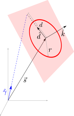
Figure 2: A schematic figure showing the the string loop in the sky and the various parameters used to describe it. The red circle is the axion string loop while the blue line shows the photon direction. $\vec{s}$ gives the location of the center of the string loop, $r$ is its radius, $\hat{k}$ is the orientation, $\hat{\gamma}$ is the direction the CMB photon is coming from, and $d$ is the distance between the photon trajectory and the loop center measured in the plane of the loop (red shaded surface).

We work in conformal time,

$$ds^{2}=a^{2}(\eta)(d\eta^{2}-d\vec{x}^{2})$$ (24)

and describe the computation in a matter dominated universe for simplicity of analytical expressions (the case with an accurate evolution history of the universe can be obtained by simply using the correct Hubble evolution $H(a)$). In this case, the comoving Hubble is

$$aH =\frac{2}{\eta}$$ (25)

We choose a comoving coordinate system with the observers at the origin. The probability density of finding a string loop with the center of the loop at coordinates ($\vec{s}$) with orientation ($\hat{k}$) and a coordinate radius of the string loop ($r$) at a time ($\eta$) is denoted as

$$P(\vec{s},r,\eta,\hat{k}) =\delta\left(r-\frac{1}{aH}\right)f(\eta)$$ (26)

where we have assumed that this probability is spatially uniform (independent of the direction of $\hat{s}$) and isotropic in $\hat{k}$. The function $f(\eta)$ can be fixed by demanding that the total energy in a given volume follow the expected scaling limit:

$$\int dr\,d^{3}\vec{s}\,d^{2}\hat{k}\ (2\pi ra)\mu(\eta)P(\vec{s},r,\eta,\hat{k})=Va^{3}\xi(\eta)\mu(\eta)H^{2}$$ (27)

where $\mu(\eta)\approx\pi f^{2}\log(f/H)$ is the string tension at time $\eta$. This implies,

$$f(\eta) =\frac{1}{4\pi}\frac{\xi(\eta)(aH)^{3}}{2\pi}$$ (28)

We are interested in the polarization rotation of a photon from a given direction $\Phi(\theta,\phi)$. We approximate the polarization rotation by assuming that the photon undergoes a polarization rotation of $\mathcal{A}\alpha_{\rm em}$ when passing through a loop and 0 otherwise. This is a good approximation for string loops that subtend a small angle on the sky and both the time of emission (CMB) and time of observation (today) can be treated as infinitely far away from the string loop, but we do not expect to recover the low-$\ell$ signal with this approximation.

To proceed, we need the condition for a photon from the direction $\hat{\gamma}$ to pass through a loop centered at $\vec{s}$, with a normal vector $\hat{k}$ and radius $r$. The distance of the photon trajectory from the center of the string loop (calculated in the plane of the string loop) is

$$d=\left|\frac{\vec{s}\cdot(\hat{\gamma}(\hat{d}\cdot\hat{\gamma})-\hat{d})}{1-(\hat{d}\cdot{\hat{\gamma}})^{2}}\right|,$$ (29)

where $\hat{d}$ is the unit vector along the radial direction of the string in the plane containing $\vec{s}$ and $\hat{\gamma}$,

$$\hat{d} =\frac{\hat{k}\times(\hat{\gamma}\times\vec{s})}{|\hat{k}\times(\hat{\gamma}\times\vec{s})|}$$ (30)

For the photon to pass through the string loop, we need $d<r$. The geometry is shown explicitly in figure 2. The total polarization rotation is given as a line-of-sight integral over the probability of the photon to pass through a given loop. We can calculate the two-point function for the polarization rotation angle as an integral over the ensemble. At a time $\eta$, the photon is at a distance $(\eta_{0}-\eta)$ from us and the strings that can contribute to the two-point function at this epoch have a distance $\vec{s}=(\eta_{0}-\eta)\hat{s}$. Thus, the two-point function can now be written analytically,

$$\langle\Phi(\hat{\gamma})\Phi(\hat{\gamma^{\prime}})\rangle =(\mathcal{A}\alpha_{\rm em})^{2}\int d\eta\int d^{2}\hat{s}\int d^{2}\hat{k}\,(\eta_{0}-\eta)^{2}f(\eta)$$

$$\qquad\qquad\qquad\qquad\times\Theta\left(\frac{\eta}{2}-d(\hat{s},\hat{\gamma},\hat{k},\eta)\right)\Theta\left(\frac{\eta}{2}-d(\hat{s},\hat{\gamma^{\prime}},\hat{k},\eta)\right)$$ (31)

where $\Theta$ is the Heaviside-theta function ensuring that the two-point function only gets contributions when both photons pass through the same loop. The picture where we think of photons as passing through small loops breaks down when the radius $r$ of the loop becomes comparable to the distance $s$ to the loop. This happens at late times when $\eta\sim\eta_{0}$. So we only expect this estimate to work for earlier times, corresponding to power at larger values of $\ell$ ($\ell\gtrsim{\rm few}$). Note that by isotropy the two-point function only depends on the angle between $\gamma$ and $\gamma^{\prime}$, or $\cos\theta=\gamma\cdot\gamma^{\prime}$. So without loss of generality we can set $\hat{\gamma^{\prime}}=\hat{z}$, and the azimuthal angle in $\hat{\gamma}$ to zero.

We present results for the two-point function computation in figure 3 and discussion of the figure in section 4.4. It is illuminating to make a further simplification to get a simple analytical estimate for the variance of the polarization rotation angle. We assume that the loops are all oriented perpendicular to our line of sight (i.e. lie on the constant $\eta$ surfaces). In this case, $\hat{k}.\hat{s}=\pm 1$. The condition for the photon to pass through simplifies to

$$(\eta_{0}-\eta)\tan\omega<\eta/2.$$ (32)

where $\hat{s}\cdot\hat{\gamma}=\cos\omega$.

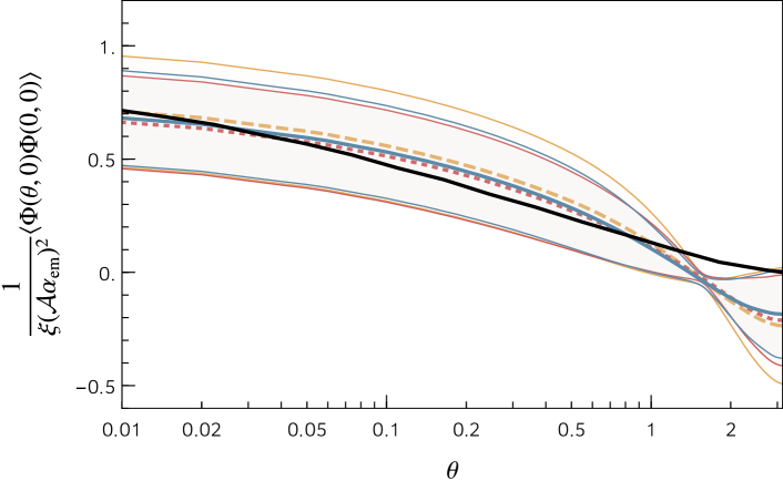
Figure 3: The two-point function of polarization rotation angle (normalized by $\xi\mathcal{A}^{2}\alpha_{\rm em}^{2}$). The black solid line is the analytical estimate calculated in the text with loops with a random normal direction compared to that of the photon trajectory. The blue solid, yellow dashed and the red dotted lines and the corresponding shaded regions show the central value and standard deviation of the two point functions from the toy simulation for $\xi=1,\,\,10,\,\,100$, respectively. The uncertainties are mainly due to cosmic variance.

The polarization rotation angle along any fixed line of sight follows a distribution where the mean is 0, and the variance is given by the two point function with $\hat{\gamma}=\hat{\gamma^{\prime}}$, or $\theta=0$. Parametrizing the center of the string with angles $(\theta_{0},\phi_{0})$, we obtain $\omega=\theta_{0}$ and the two-point function does not depend on $\phi_{0}$, so that

$$\langle\Phi(0,0)\Phi(0,0)\rangle =2\pi(\mathcal{A}\alpha_{\rm em})^{2}\int dc_{\theta 0}d\eta(\eta_{0}-\eta)^{2}\frac{(aH(\eta))^{3}\xi(\eta)}{2\pi}\Theta\left(\frac{\eta}{2}-(\eta_{0}-\eta)\tan\theta_{0}\right)$$ (33)

$$\approx\xi(\mathcal{A}\alpha_{\rm em})^{2}\log\left(\frac{\eta_{0}}{\eta_{\rm CMB}}\right)\,.$$ (34)

In the second line we have only kept the leading $\log$ behavior. This estimate agrees with the intuition that a photon goes through about $\xi$ string loops per Hubble time in its trajectory when there are $\xi$ loops per Hubble patch. The polarization itself is undergoing a random walk with $N=\xi\log\left(\eta_{0}/\eta_{\rm CMB}\right)$ steps and a step size of $\mathcal{A}\alpha_{\rm em}$. This analytic estimate shows good agreement with the numerical results.

The analytical method we described can also be used to capture the leading behavior of the higher point correlation functions. The higher point functions come about when multiple photons pass through the same loop. As a result, we expect the $N$-point correlation functions of $\Delta\Phi$ to scale as $\xi(\mathcal{A}\alpha_{\rm em})^{N}$. All the odd correlation functions, for example the 3-point function, are zero at leading order after integrating over both orientations of the string loops. The absence of a 3-point function and the scaling of higher point functions with $\alpha_{\rm em}$ allows us to distinguish our signal and potentially measure $\mathcal{A}\alpha_{\rm em}$ and $\xi$ separately from the correlation functions.

The above analytical analysis can be extended to the case when the axion is massive. When a photon passes through a domain wall $\Delta\Phi=\pm\mathcal{A}\alpha_{\rm em}/N_{\rm DW}$. Since each string has $N_{\rm DW}$ domain walls attached to it, traveling around a string with or without domain walls, one always obtains the same polarization rotation angle of $\Delta\Phi=\pm\mathcal{A}\alpha_{\rm em}$ and as a result, the previous results do not change significantly. When the domain wall number $N_{\rm DW}\neq 1$, the $Z_{N_{\rm DW}}$ symmetry is exact and hence the string-domain wall network is stable, the previous analysis still applies. In fact, as we will discuss in more detail in subsection 4.4, the quantized nature of the signal at CMB will actually improve if domain walls form. The case where the $Z_{N_{\rm DW}}$ symmetry is significantly broken or $N_{\rm DW}=1$ is more involved.

If the axion mass is in the range

$$H_{0}\lesssim m_{a}\lesssim H_{\rm CMB},$$ (35)

the axion domain walls will form during the period when the CMB photons are propagating to us. The formation of the domain wall and the subsequent disappearance of the axion string network as the universe expands means that the larger string loops at late times do not exist, leading to a suppression of power at large angular scales. Practically speaking, this effect comes from limiting the $\eta$ integral to only extend to the time when the strings disappear. The string-domain wall network will emit most of its energy into ambient axion density. The exact form of the correlation functions that results from the axion radiation will depend on the spectrum of the axion radiation. However, we expect that the small angle correlations ($100\gtrsim\ell\gtrsim{\rm few}$ modes of the CMB) will follow our analytic predictions. Meanwhile, the power in small $\ell$ modes ($\ell$ corresponding to the time when domain walls annihilate) may be affected by the axion radiation coming from the annihilation of the string-domain wall network. A dedicated simulation of the evolution of the axion string-domain wall network in this case will be extremely helpful for predicting the signal shape.

4.3 A toy numerical simulation

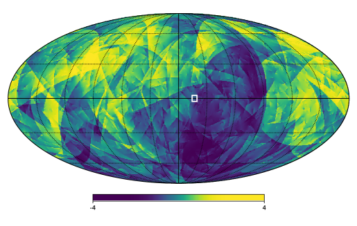
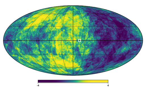
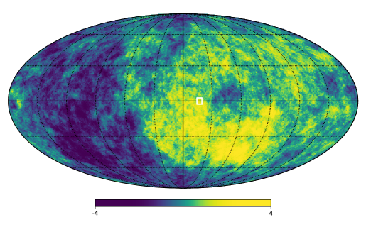
Figure 4: The polarization rotation angle map $\Phi(\hat{\gamma})$ for photons from a simulation of axion strings described in the text. The three figures, from top to bottom, have the number of string per Hubble patch $\xi=1,10,100$ respectively. The rotation is normalized by $1/(\sqrt{\xi}\mathcal{A}\alpha_{\rm em})$ and is measured in radians. The contribution from long strings today is clearly visible. The white boxes mark the boundary of the region shown in figure 7.

The calculation above captures the contributions from Hubble sized loops between $z$ of a few and the CMB, but fails to capture the late-time behavior. In particular, there should be low-$\ell$ signals from strings in the current universe, including spatial features in the CMB that we can look for. We employ a simplified numerical simulation of strings to understand this effect. This simulation is a toy set up that we hope captures the qualitative properties of the signal. An obvious next step for future work would be to use dedicated axion string network simulations to verify the claims made in this paper. An encouraging sign is that the results of the analytical calculation above agree with the toy simulation for $\ell\gtrsim{\rm few}$.

The simulation assumes that all strings are straight and infinite in length. This is an oversimplification of the string structure, which is expected to have structure at the Hubble scale. However, this effect is mitigated by the presence of multiple other strings with random orientation within a Hubble volume. Further, strings are assumed to be static so that we do not model the string motion. We populate a box of size $5\times(1/H_{0})$ with strings at random positions and random orientations uniformly. In order to keep the scaling limit as time progresses,

$$\rho_{\rm strings} =\xi\mu H^{2},$$ (36)

at every time step an appropriate number of strings are discarded at random.

In this network of strings, we simulate photon trajectories starting from the surface of last scattering (which we take to be a thin sphere centered at our position) from various angles, and calculate the polarization rotation angle along its line of sight. This is done by assuming an axion profile around the string to be $\nabla a=\frac{1}{r}\hat{\phi}$, where $\hat{\phi}$ is the azimuthal direction when the string points towards the positive $z$ direction.

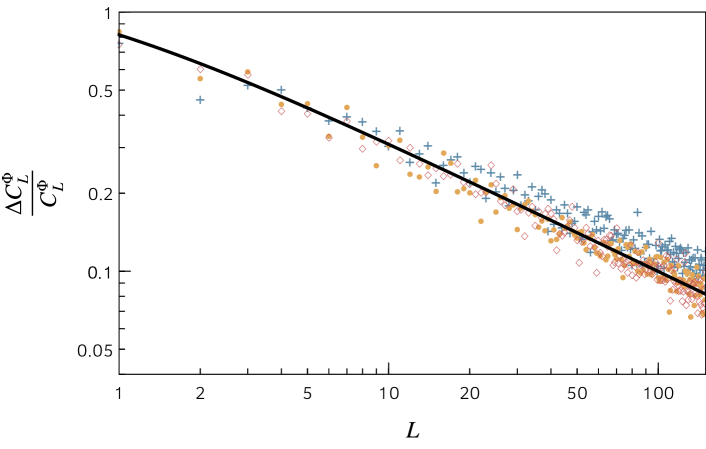
Figure 5: $\Delta C_{L}^{\Phi}/C_{L}^{\Phi}$ as a function of $L$. $\Delta C_{L}^{\Phi}/C_{L}^{\Phi}$ is the ratio between the standard deviation and the mean of $C_{L}^{\Phi}$ from the simulations with different choices of $\xi$. The blue, yellow and red markers show the value of $\Delta C_{L}^{\Phi}/C_{L}^{\Phi}$ from our simulations with $\xi=1,\,\,10,\,\,100$, respectively. The black solid line is the expected cosmic variance value of $\Delta C_{L}^{\Phi}/C_{L}^{\Phi}=\sqrt{\frac{2}{2L+1}}$. These results come from 60 simulations per value of $\xi$.

We show the polarization rotation obtained in this manner in figure 4. The presence of string-like structures is clearly visible. We can further compute the two-point function and the $C_{\ell}$ from this map, where

$$C_{\ell}^{\Phi}=2\pi\int d\cos\theta\,\langle\Phi(\cos\theta)\Phi(0)\rangle P_{\ell}(\cos\theta)$$ (37)

is the usual definition. In figure 3, we show the result and uncertainty of the two point correlation of polarization rotation angle as a function of angular scale $\theta$ and $\phi$ from our toy numerical simulation. Note that the feature that all the curves approximately pass through 0 for $\theta=\pi/2$ is a consequence of the power spectrum being dominated by the dipole in the straight string case. As our analytical estimate shows, this suppression is not universal when the strings are not straight.

The toy simulation also offers an opportunity to understand the variance of the expected signal. The overall amplitude of the signal, as shown in figure 3, varies from simulation to simulation. These variations are mainly due to the effect of strings at low-$z$, which in $\ell$-space, become variations of $C_{\ell}$ at low $\ell$. In figure 5, we show the size of these variations as a function of $\ell$, which matches with the expectation that the variance is entirely due to cosmic variance. In the rest of the paper, we will simply treat our sensitivity as cosmic variance limited.

4.4 Method comparison and limitations

In this section, we have shown two methods that we used to compute the two point function of the polarization rotation angle. The two methods agree very well at small values of $\theta$ but differ at large angular scales (see figure 3). This arises from the fact that the analytical analysis does not take into account the long strings present in the current epoch. These long strings will contribute to correlations at a very large angular scale and small $\ell$ ($\ell\sim 1$). The toy simulation captures the large dipole contribution from these strings stretching across the sky. However, as shown in figure 5, at small $\ell$, our prediction is cosmic variance limited. The analytical method might also overestimate the effect coming from the string loops that are either very close to the surface where CMB photons are emitted or very close to the detector. For these string loops, treating the CMB photons as originating from and ending at infinitely far away leads to an over-estimate of the total phase accumulated by the CMB photons, which might also lead to a difference between the analytical calculation and numerical simulation.

The good agreement of the two methods at small angular scales is encouraging since treating strings as a circular loop versus infinitely long straight lines are two extremely different ways of modeling the shape of strings in our universe. Getting comparable results for the two cases suggest that the uncertainty coming from the evolution of the string network should be small. However, precise predictions of polarization rotation from an axion string network extracted from a dedicated numerical simulation will provide valuable information about the evolution of the network as the universe transitions from radiation domination, to matter domination, to CC domination today, and will be crucial for confirming the nature of the signal in light of an observation. On the other hand, an experimental measurement of strings will give us information about the total string length per Hubble as well as the domain wall number $N_{\rm DW}$. This information would be very useful for clarifying the evolution of the string network or string-domain wall network, in particular the deviation from a scaling solution, in more general scenarios.

On the CMB side, we have not taken into account two issues that can make the analysis more involved. First, the CMB photons are not emitted all at the same redshift Hu:1997hv . CMB photons emitted from the same angular direction at different $z$ can have slightly different polarization rotation angles. The effect is largest for the string closest to the surface of last scattering, which will cause a difference in the polarization rotation angle of $\Delta\Phi\propto\xi\Delta z/z$ where $\Delta z\sim 200$ is the width of the surface of last scattering. We can estimate the change in the two-point function shown in equation (33) by taking one of the many strings and giving it a rotation $\Phi=\mathcal{A}\alpha_{\rm em}(1-\xi\Delta z/z)$, as opposed to the usual $\mathcal{A}\alpha_{\rm em}$, to arrive at

$$\frac{\Delta\langle\Phi(0,0)^{2}\rangle}{\langle\Phi(0,0)^{2}\rangle}\sim\frac{\Delta z}{z_{\rm CMB}}\frac{1}{\log\left(\eta_{0}/\eta_{\rm CMB}\right)}\sim 1\%$$ (38)

so that this is not expected to be a significant effect. Secondly, the polarization rotation angle power spectrum receives some additional contribution from the period of reionization at low $\ell$. These new contributions to the CMB polarization will only be affected by the large string loops present at late time, and will as a result, have a different rotation angle as compared to the polarization generated around the time of recombination. The contributions to the CMB polarization during the epoch of reionization is significant at low $\ell$ (e.g. it is dominant for $\ell\lesssim 10$ for $E$-mode polarization). A robust prediction of the correlation functions at low $\ell$ will require a dedicated simulation. However, we do not expect it to significantly change the qualitative features since the polarization generated around reionization still goes through $\mathcal{O}(1)$ of the total string loops. In fact, the ratio of the polarization rotation angle of the polarization generated during reionization (lower-$\ell$) and recombination (higher-$\ell$) can be an interesting cross check in light of a discovery. We leave these issues to a more dedicated analysis in the future.

When axions are massive compared to $H_{0}$, the strings and domain walls have a very different evolution history, as outlined in section 4.1. However, the observable signal does not change significantly in the case where $N_{\rm DW}\neq 1$. In fact, an axion mass that is larger than $H_{\rm CMB}$ will reduce many of the uncertainties we have coming from the issues mentioned before, since the formation of the axion domain wall will shrink the region of space where the axion field is varying and as a result, reduce the fraction of photons that are emitted in the region where the axion field is changing. This would be especially helpful if we use the CMB to determine the value of the quantized polarization rotation angle from a single string. As mentioned before, if $N_{\rm DW}=1$, the string network will disappear when the domain walls form and the energy density stored in the string-domain wall network is converted to axion radiation.

Another limitation of our simple analysis comes from the ambient axion density emitted by the string (and domain wall) network. The ambient density of axions emitted by this network have properties similar to those coming from a misalignment mechanism, which was studied in detail in Fedderke:2019ajk . The two effects of the axion radiation are a rotation of the polarization due to the differences in the axion field value from the time of CMB to today, and a reduction of the $E$-mode polarization due to smearing by the differing axion field values during the time of the emission of CMB photons. The smearing effect is maximal when the frequency of oscillation of the axion is fast compared to the duration over which the CMB is emitted. As the spectrum of axions emitted by the string network is not reliably known yet, we estimate the strongest that this bound could be by assuming that all of the axion radiation is oscillating fast and at the same frequency. The constraint in our normalization is that

$$\frac{\mathcal{A}\alpha_{\rm em}}{\pi}\frac{a}{f}\leq 0.15$$ (39)

coming from the Planck polarization measurement Fedderke:2019ajk . Taking the energy in axion radiation to be the same as in the strings, we find that $\mathcal{A}\lesssim\mathcal{O}(10)$. Unlike effects coming from strings, the polarization rotation coming from the axion radiation is not enhanced by square-root of the number of strings in between CMB and today ($\sqrt{N_{s}}$). As a result, we do not expect them to cause any qualitative change to the correlation functions we predict. However, the ambient background of axions may act as noise and inhibit our ability to identify a single string and measure the quantized polarization rotation angle around the string.

5 CMB Observables

In this section, we present how the polarization rotation coming from string networks map onto CMB observables. We first review how the polarization rotation angle power spectrum is calculated from the CMB maps and compare current constraints and forecasts with the predictions from our simulations described in section 4. Afterwards, we discuss features of our signal that would allow it to be separated from backgrounds. The most interesting feature of string networks are the discontinuities in the polarization direction that appear in the sky. Throughout this section, we will use capital letter $L$ and $M$ when describing the polarization rotation angle $\Phi$ specifically and small letters $l$ and $m$ when describing the CMB E- and B-modes specifically. We will keep using the letter $\ell$ for general discussion.

5.1 Polarization rotation angle power spectrum

We denote the birefringence rotation as $\Phi(\hat{\gamma})$, as before. The cosmic birefringence leaves the temperature field and the size of the polarization unchanged and rotates the polarization angle. This corresponds to changing the Stokes parameters as follows,

$$p(\hat{\gamma}) =Q(\hat{\gamma})\pm iU(\hat{\gamma})=(\tilde{Q}(\hat{\gamma})\pm i\tilde{U}(\hat{\gamma}))\exp(\pm 2i\Phi(\hat{\gamma}))$$ (40)

where $\tilde{Q},\tilde{U}$ are the Stokes parameters in the absence of birefringence. Since $U$ is parity-odd and $Q$ is parity-even, this rotation breaks parity. In terms of $E$- and $B$- mode decomposition,

$$p(\hat{\gamma}) =\sum_{lm}(E_{lm}+iB_{lm})_{2}Y_{lm}(\hat{\gamma})$$ (41)

where ${}_{2}Y_{lm}$ are the spin-2 spherical harmonics. The polarization rotation converts E-modes into B-modes in a $\ell$ dependent way. Since the primordial $B$-modes have been constrained to be far smaller than the $E$-modes, the dominant signal comes from generation of $B$-modes Contreras:2017sgi ; Gluscevic_2012 ,

$$B_{lm} =2\sum_{LM}\sum_{l^{\prime}m^{\prime}}\Phi_{LM}E_{l^{\prime}m^{\prime}}\Xi^{LM}_{lml^{\prime}m^{\prime}}H^{L}_{ll^{\prime}}$$ (42)

with $\Xi$ and $H$ are associated with Wigner-3$j$ symbols,

$$\Xi^{LM}_{lml^{\prime}m^{\prime}} \equiv\frac{(-1)^{m}}{4\pi}\sqrt{(2l+1)(2l^{\prime}+1)(2L+1)}\left(\begin{array}[]{ccc}l&L&l^{\prime}\\ m&M&m^{\prime}\end{array}\right)$$ (45)

$$H^{L}_{ll^{\prime}} \equiv\left(\begin{array}[]{ccc}l&L&l^{\prime}\\ 2&0&-2\end{array}\right)$$ (48)

and we have expanded the polarization rotation angle in spherical harmonics, $\Phi(\hat{\gamma})=\sum_{LM}Y_{LM}(\hat{\gamma})\Phi_{LM}$. The summation is restricted to even values of $L+l+l^{\prime}$. This reflects the unique parity violating nature of birefringence. For example, $B$-modes generated by lensing $E$-modes only get contributions from the odd values of the sum, and thus can be distinguished from our signal.

This can be used to build an estimator $\hat{\Phi}_{LM}$ for the polarization rotation angle Gluscevic:2009xxx ; Gluscevic_2012 , for example

$$[\hat{\Phi}^{E^{i}B^{j}}_{LM}]_{ll^{\prime}} =\frac{2\pi}{(2l+1)(2l^{\prime}+1)C_{l}^{EE}H_{ll^{\prime}}^{L}}\sum_{mm^{\prime}}B^{i}_{lm}E^{j*}_{l^{\prime}m^{\prime}}\Xi^{LM}_{lml^{\prime}m^{\prime}}\,.$$ (49)

The minimum variance estimator combines estimates from all such channels, $\{E^{i}B^{j},B^{i}E^{j},T^{i}B^{j},B^{i}T^{j}\}$, where $i,j$ index channels for a given map.

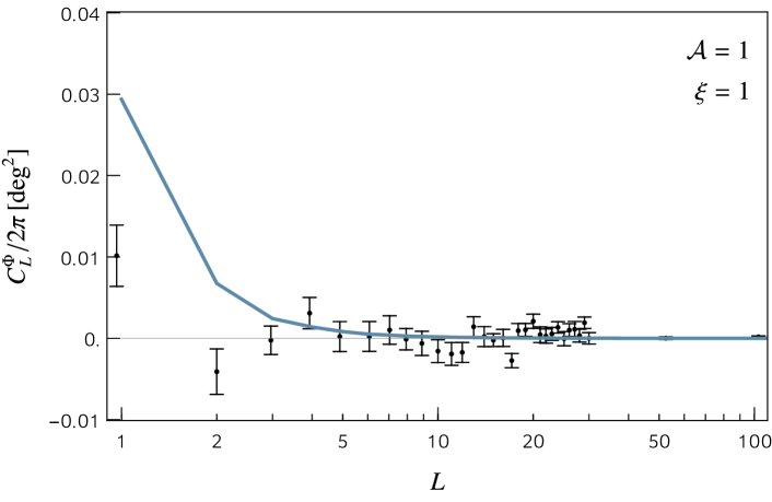
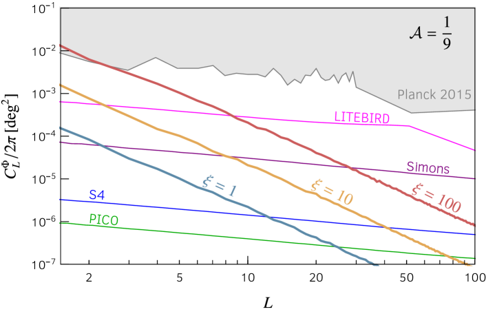
Figure 6: Power spectrum of the polarization rotation angle. Top: Constraints on the power spectrum derived from Planck 2015 polarization data (data points) Contreras:2017sgi . The blue curve shows the power spectrum for $\xi=\mathcal{A}=1$, which is of the order of the current sensitivity. Bottom: Forecasts for the power spectrum measurements in future experiments Pogosian:2019jbt . The grey shaded region is excluded by Planck while the thin magenta, purple, blue and green lines show the sensitivity of future CMB experiments. The thick blue, yellow and red solid lines show the prediction for $\xi=1,\,10,\,100$ and $\mathcal{A}=1/9$. For both plots we have taken a mean over cosmic variance for our prediction. The power spectra can be scaled for other values of $\xi$ and $\mathcal{A}$ as $C_{L}^{\Phi}\propto\xi\mathcal{A}^{2}$.

The variance in the estimator is given as,

$$\langle\hat{\Phi}_{LM}\hat{\Phi}_{L^{\prime}M^{\prime}}\rangle =\delta_{LL^{\prime}}\delta_{MM^{\prime}}(C_{L}^{\Phi}+\sigma^{2}_{\Phi,L})\,,$$ (50)

where $\sigma^{2}_{\Phi,L}$ is the combined variance of the estimators, and $C_{L}^{\Phi}$ is the power spectrum of the polarization rotation angle due to birefringence. The variance $\sigma^{2}_{\Phi L}$ includes contributions from the beam systematics, detector noise, galactic and atmospheric foregrounds and weak lensing contribution. This variance can then be used to forecast sensitivity to $C_{L}^{\Phi}$,

$$\sigma_{C_{L}^{\Phi}} =\frac{\sigma^{2}_{\Phi,L}}{f_{\rm sky}(2L+1)/2}\,.$$ (51)

The details of the sky coverage $f_{\rm sky}$, delensing fraction, beam parameters and sensitivity used for different experiments in figure 6 can be found in Pogosian:2019jbt . The current CMB constraints are sensitive to a constant birefringence rotation of $0.5^{\circ}$ at $1\sigma$ level, which is roughly of the expected size $\Phi\simeq\alpha_{\rm em}$ for $\xi=1$ and $\mathcal{A}=1$. In figure 6 (top) we plot the $C_{L}^{\Phi}$ values obtained in our simulation (for $\xi=1$, $\mathcal{A}=1$) against the $C_{L}^{\Phi}$ constraints derived in Contreras:2017sgi from Planck. We also plot future sensitivity ($\sigma_{C_{L}^{\phi}}$) for various future experiments Pogosian:2019jbt (bottom). The orthogonality with the lensing signal implies that the optimal sensitivity is obtained for measurements around the peak of the E-mode spectrum, $500<\ell<3000$. Higher resolution does not lead to better sensitivity to the rotation power spectrum since the polarization signal is smaller at smaller scales. However, as we will see below, higher resolution can help resolve the strings directly in position space.

It is intriguing to note that there is an excess dipole signal in the data. If this is a signal of a string, it may be possible to find further evidence for it in the newly released Planck 2018 data. Future experiments will have improvement in sensitivity by orders of magnitude, which can definitively probe a signal coming from $\xi,\mathcal{A}\sim 1$ string networks.

5.2 Distinguishing strings from other sources of B-modes

In this section, we briefly address the distinguishability of our signal from other sources of B-mode polarization. Our signal, as shown in figure 6, will have a particular $\ell$-dependence, which can potentially be distinguished from B-modes coming from other sources. Moreover, we expect our effect to have a distinct structure when we consider higher point correlation functions. In particular, we expect the 3-point correlation function and all odd correlation functions are zero at leading order, and all the even $N$-point correlation functions to have a scaling with $\xi$ and $\mathcal{A}\alpha_{\rm em}$ as $\xi(\mathcal{A}\alpha_{\rm em})^{N}$. Furthermore, there are two other main features of our signal at the level of two point correlation functions of $\Phi$ in the CMB, parity violation and frequency independence.

Lensed B-modes

The lensing of $E$-modes produces correlated $B$ modes in the CMB spectrum. This leads to parity conserving correlators, and hence are distinguishable to the axion induced birefringence signal.

Primordial Gravitational Waves

Primordial gravitational waves induced by high scale inflation are a prime target for CMB experiments. The gravitational waves induce a $B$-mode spectrum, but not a parity violating $EB$ correlators in most inflation models 1985SvA….29..607P ; Seljak:1996gy ; Kamionkowski:1996zd ; Seljak:1996ti . In specific models Anber:2012du ; Adshead:2013qp ; Thorne:2017jft , the spectrum of gravitational waves induced can be chiral which leads to parity-violating fluctuations in the CMB. These models come with a rich set of associated signals such as non-gaussianities, and we expect that detailed properties of the power spectrum and higher-point functions will readily distinguish this signal from axion strings.

Faraday rotation

Primordial magnetic fields generate a Faraday rotation of the CMB polarization, converting E modes to B modes. Such a primordial magnetic field is motivated by observation of $\mu$G galactic magnetic fields whose origin is not well-understood. The spectrum of the polarization rotation angle induced by these magnetic fields depends on their power spectrum. Faraday rotation has a distinctive frequency dependence, $\Phi\sim\nu^{-2}$, and hence it will be very easily distinguished from an axion string induced rotation.

Lorentz violation

Cosmic Birefringence was in fact first proposed Carroll:1989vb in the context of measuring Lorentz violating terms in the SM. In the SM extension formalism, the $d=3$ terms associated with a Chern-Simons-like coupling is physically equivalent to an axion background with a uniform gradient. Higher dimensional terms produce frequency dependent terms. Therefore, it will be relatively easy to disentangle effects of such terms from an axion string network.

We see that even at the statistical level, it will likely be possible to disentangle our signal from other potential sources of parity-odd $B$-modes in the CMB. However, the spatial morphology of the signal from strings, with a $\sim\mathcal{A}\alpha_{\rm em}$ jump across the strings, is a smoking gun feature which sets apart the axion string signal. This is the signal we now turn to.

5.3 Edge detection

Cosmic strings are distinctive features in position space, so analyzing the signal in Fourier space may not be the optimal strategy to study the properties of the strings. For this reason, it would be interesting to look for the strings directly in position space. For the case of gravitational effects of cosmic strings, edge detection algorithms for the CMB temperature maps Stewart:2008zq have been proposed.

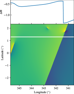
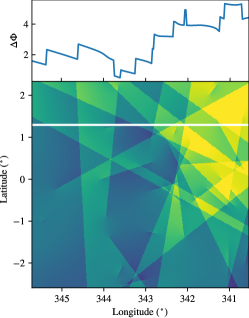
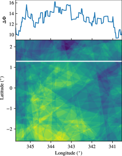
Figure 7: Zoomed-in skymaps at the truth-level for $\xi=1,10,100$ showing the white framed areas in the respective skymaps in figure 4 (the color scale is modified for visual clarity). The presence of sharp discontinuities is apparent in these images of broken light. The discontinuity is quantized and is equal to 1. The white stripe shows a slice through the map, and the value of $\Delta\Phi$ (normalized by $1/(\mathcal{A}\alpha_{\rm em})$) is shown in the top panels where the quantized jump is apparent.

The polarization rotation angle of the photons has a discontinuity across the axion string. A similar edge detection algorithm can be developed to detect this discontinuity in polarization maps. The value of the discontinuity is an extremely interesting quantity to measure. The two path across the string differ by a path that loops around the string, and hence measures the topological charge of the string (see section 3).

In figure 7, we show a zoomed-in patch of our simulation, where the discontinuity is apparent. To develop this edge detection algorithm for polarization maps will be an extremely interesting future direction. The size of the discontinuity contains a wealth of information, as we have said, so to extract that would be important. Edge detection can potentially be used to look for a single string in the entire universe, or strings that are even beyond our horizon Kaplan:2008ss , both corresponding to cases where the $U(1)$ symmetry is broken before inflation.

The two main limiting factors on edge detection are the angular resolution of the experiment and the precision of polarization measurement. Ground-based observatories like The Atacama Cosmology Telescope (ACTPol) Thornton:2016wjq , South Pole Telescope 2011PASP..123..568C , POLARBEAR 2012SPIE.8452E..1CK , and future Simons Observatory Ade:2018sbj will have the ability to measure polarizations at arcmin angular scales. This corresponds to a sensitivity in the range $\xi\lesssim 100$ such that the angular separation between strings is larger than the angular resolution. The Simons Observatory Ade:2018sbj has a noise-level of $\sim{\mu{\rm K}}$-arcmin, and the ability to measure polarization rotations to $\mathcal{O}({\rm deg})$. Improvements of both the angular resolution and noise-level would improve the sensitivity to axion strings with edge detection 2018SPIE10700E..5XP ; Sehgal:2019ewc . In figure 10, we show a very rough estimate of the sensitivity to axion strings using edge detection with current technology and leave a dedicated analysis to future work. How the sensitivity scales with $\xi$ is not very clear because, on one hand, having more strings requires better angular resolution and smaller noise at small angular scales, while on the other hand, having more strings also increases the statistics. Edge detection in 2d images is a prime application for machine learning algorithms. Since our signal lives precisely in this space, it may be an ideal candidate to apply some of these deep learning technologies to. It is a very interesting future direction to study edge detection techniques to find individual strings in the presence of complications such as reconstruction noise.

6 Other observational signature of axion strings

In this section, we discuss some of the other signatures of an axion string due to its coupling with the photon. We also discuss the signatures that come purely from the gravitational coupling of the axion strings and domain walls. These include their gravitational effect on the CMB as well as gravitational wave emission during the string network evolution. We collect all these constraints and future sensitivities in figure 9.

6.1 Quasar lensing

The axion string network can also be looked for with distant gravitationally lensed polarized light sources. A particular example of such a source is a quasar. Recently, many strongly gravitationally lensed quasars have been found and carefully measured to extract valuable information about the expansion history of our universe by the H0LiCOW collaboration Suyu:2016qxx . These strongly lensed quasars, with multiple images and image separations as large as $\beta\sim 20^{\prime\prime}$ Inada:2003vc (see glqdatabase for a list of 205 known gravitational lensed quasars), can also provide very unique information about cosmic axion strings.

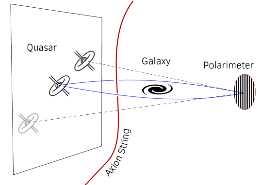
Figure 8: A quasar at a cosmological distance is gravitationally lensed by a galaxy or galaxy cluster in between the quasar and the observer. The different photon trajectories (blue lines) from the quasar to the observer, corresponding to different quasar images, form a closed loop around the gravitational lens. An axion string (red line) can pass through this closed loop of photon trajectories, leading to a differential polarization rotation angle between the two photon trajectories (quasar images).

As shown in figure 8, a lensed quasar can have multiple images with angular separation $\beta$. The area enclosed by the two photon trajectories is roughly

$$A_{\rm enc}\simeq D_{L}D_{S}\beta/2,$$ (52)

where $D_{S}$ and $D_{L}$ is the distance to the source and the lens, respectively. If the enclosed area is pierced by an axion string, the two observed image will have a relative rotation between the polarization of their images. As before, this rotation will be quantized. In the case of the CMB, the approximately quantized nature of the signal stems from the fact that for most string loops are at an intermediate redshift, and the CMB photon can be treated as either traversing through a loop or not. In contrast, the quantized nature of the lensed quasar signal comes from the fact that the two photon trajectories combine to actually form a closed curve. This makes gravitational lensed quasars, and other strongly lensed distant objects unique systems to test the existence of these axion strings. The probability for an axion string to traverse this area is

$$p\simeq\xi A_{\rm enc}H_{0}^{2}\approx 10^{-3}\frac{\xi}{100}\frac{\beta}{10^{\prime\prime}},$$ (53)

for each lensed quasar that is at a cosmological distance.

Measurement of the polarization of distant quasars have been made in the optical 1990ApJ…354..124I ; Sluse:2005bg ; 1998A&A…340..371H and the radio frequency range Taylor_1998 ; Taylor:1999ms . The polarization uncertainties in this frequency range are at the degree level, mainly coming from calibration, which can potentially be improved when measuring relative polarization of two quasar images. Our signal is a quantized polarization rotation at the % level or smaller. Current easily accessible technology for measuring the polarization of optical frequency photons is around the $\sim 10^{-5}$ level 2017MNRAS.465.1601B . Thus, future observations of lensed polarized quasars can complement the search with the cosmic microwave background, and have the unique ability to test the quantized nature of the observed signal. It will be very interesting to perform detailed projections for searches with lensed quasars. We leave this for future work.

The distinguishability of our signal from background relies on two important properties of the signal coming from a topological defect. The topological nature of the signal ensures that the polarization rotation angle is quantized. As a result, different pairs of lensed quasar images, as well as different lensed quasar systems, will have the same relative polarization rotation up to an integer multiple. The topological nature of the signal also ensures that the polarization rotation angle is frequency independent, which helps when distinguishing our effect from that of Faraday rotation along different trajectories. The axion strings we can look for with quasar lensing will have lengths that are comparable to the size of the universe today and will also leave an imprint on the cosmic microwave background, providing another unique cross check in the case of a discovery.

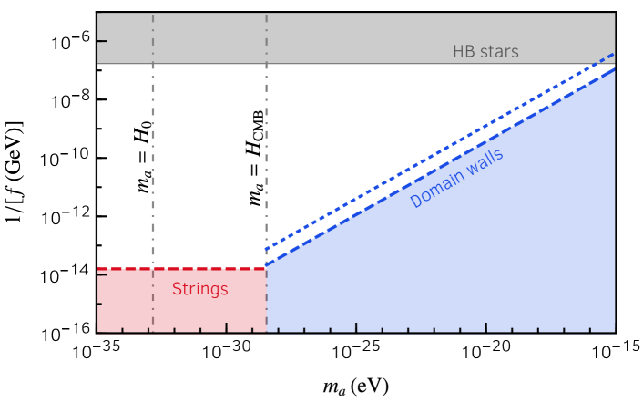
Figure 9: Parameter space for polarization rotation and gravitational wave signatures. The gray shaded region is excluded by cooling bounds coming from Horizontal Branch stars Ayala:2014pea (assuming $\mathcal{A}=1$). The red shaded region is excluded by CMB measurements of strings coming from their gravitational effects Charnock:2016nzm . The blue region is excluded when $N_{\rm DW}\neq 1$ due to the temperature fluctuations induced by the gravitational potential of the domain wall Sousa:2015cqa . Dashed and dotted lines correspond to $\xi=10$ and 100 respectively. The figure is cut off at large $f$, as for $f\gtrsim 10^{16}\,{\rm GeV}$, the universe can not reheat to high enough temperature so that strings might not be produced. Our sensitivity applies to $\xi\geq 1$ in all of the allowed parameter space in this plot.

6.2 Gravitational and gravitational wave signatures

The strings and domain walls can also be looked for through their gravitational effect on the large scale structures of the universe. The measurement of the detailed features of, in particular, the cosmic microwave background spectrum place a constraint on the amount of density inhomogeneities that can be generated by cosmic strings Bevis:2007gh ; Battye:2010xz and domain walls. These considerations place an upper bound on the energy per unit length of the string $\mu$ Charnock:2016nzm ,

$$G\mu\lesssim 1.1\times 10^{-7},$$ (54)

corresponding to an axion decay constant $f$ no higher than $\sim 10^{14}\,{\rm GeV}$. Such a constraint on the axion decay constant is only mildly dependent on the deviation from scaling solution (see the discussion around equation (20) in section 4.1).

Similar constraints can be placed on the tension of domain walls. The energy density in the form of domains walls in a frustrated string-domain wall network approach a scaling limit Hiramatsu:2012sc ; Hiramatsu:2013qaa for $N_{\rm DW}\neq 1$,

$$\rho_{\rm wall}\approx N_{\rm DW}\sigma H,$$ (55)

where $\sigma\sim 8m_{a}f^{2}$ is the tension of the domain wall Saikawa:2017hiv . Measurements of the cosmic microwave background place a constraint on the tension of the domain walls Sousa:2015cqa

$$N_{\rm DW}G{\sigma}L_{0}\leq 5.6\times 10^{-6},$$ (56)

where $L_{0}\approx 1/H_{0}$ is the characteristic size of the domain wall today. This is an updated version of the famous Zel’dovich-Kobzarev-Okun bound of ${\sigma}\lesssim\mathcal{O}({\rm MeV^{3}})$ Zeldovich:1974uw .

Similar to the case of cosmic strings, the frustrated string-domain wall network can also have densities that deviate logarithmically from the scaling solution when the density of strings and domain walls are comparable. It is unclear if such deviation would persist when the domain wall energy density dominates that of the strings at late time. In figure 9, we show the constraints from gravitational measurement of the string-domain wall network assuming that the string-domain wall network deviates from a scaling solution logarithmically, similar to that of a string network.

The string network and the string-domain wall network emit gravitational waves as they evolve in time. The energy density and spectrum of gravitational waves from a string network have been studied extensively in the literature Vilenkin:1981bx ; Vachaspati:1984gt ; Battye:1994au (see Cui:2018rwi for more details). Future gravitational wave detectors can probe an axion decay constant as small as $\sim 10^{15}\,{\rm GeV}$ at intermediate frequencies (LISA) and $\sim 10^{14}\,{\rm GeV}$ at low frequencies (SKA) Chang:2019mza . The string-domain wall network can produce gravitational waves as it redshifts as well as when domain walls collide or annihilate. The gravitational wave signals associated with these domain walls are observable only in regions of parameter space where the domain walls annihilate at a very early time Saikawa:2017hiv and occupy a range of parameter space very different from what we are probing.

7 Conclusion

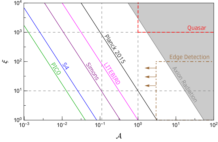
Figure 10: We show the sensitivity of current and future experiments to the two independent parameters of an axion string network with a photon coupling; the number of axion string per Hubble volume ($\xi$) and the strength of the axion string-photon coupling ($\mathcal{A}$). The CMB polarization correlation functions provide the best channel for discovery (they put an upper bound on the combination $\xi\mathcal{A}^{2}$). The black solid line is the estimated current sensitivity of Planck to this effect while the magenta, purple, blue and green lines show the sensitivity of future CMB experiments. We take the sensitivity at $L=10$ from figure 6 as an indicator. The grey region is the estimated constraint coming from the effects of axion radiation emitted from the string network, see the discussion around equation (39). CMB experiments with good angular resolution and lensed quasar systems provide an opportunity to exploit the quantized nature of our signal. The brown dot-dashed line shows the prospects for edge detection with experiments similar to the Simons observatory (very qualitative). Increasing the accuracy of the polarization rotation angle measurement improves the sensitivity to smaller $\mathcal{A}$ and improving the angular resolution improves the sensitivity to higher $\xi$. The red dashed line shows the prospects for lensed quasar systems (qualitative). Increasing the number of lensed quasars improves the sensitivity to smaller $\xi$ while improving the precision of the measurement of the relative polarization of the quasars improves the sensitivity to smaller $\mathcal{A}$. The gray dashed gridlines mark the regions of parameter space of particular theoretical interest.

String theory has reinforced the motivation for many phenomenological paradigms at low energies, two of which are cosmic strings Witten:1985fp ; Polchinski:2004hb ; Copeland:2003bj ; Copeland:2004iv ; Polchinski:2004ia and light bosonic states (axiverse) Arvanitaki:2009fg ; Demirtas:2018akl . In this paper, we have shown that these are amusingly connected to each other: the axion-photon coupling offers a unique way to look for cosmic strings, while cosmic axion strings also offer a unique way to look for axiverse axions.

Due to the extended nature of cosmic axiverse strings and the topological interaction between the strings and photon shown in equation (1), measurement of cosmic axiverse strings provide a unique opportunity to probe the UV dynamics of the theory. Measurement of the UV anomaly coefficient $\mathcal{A}$ can teach us about fundamental physics such as the smallest unit of electric charge. Aside from being theoretically fascinating, cosmic axiverse strings are also exciting phenomenologically. The basic way of searching for cosmic axiverse strings using photons is that the polarization direction of linearly polarized light rotates by a quantized amount when a photon circles a string. If the UV theory only has unit electrically charged particles, this quantized rotation will be of order a percent. If the UV theory is SM-like in its charge assignments, then the quantized rotation will be larger than $0.1\%$.

One of the most interesting ways in which this quantized rotation can be measured is using the CMB. The CMB provides a backlight which shines upon all of the strings. The difference in paths for photons passing to the left and to the right of the string is a loop around the string; thus the relative polarization rotation angle of the photons is quantized. The effect of strings on polarization can be searched for using a standard angular decomposition (power spectrum) with the Planck satellite and future CMB missions. What is perhaps more exciting is the fact that the polarization map contains discontinuities at the location of the strings, which can be looked for using edge detection techniques with ground-based missions. Finding these strings in position space and their associated discontinuities provides a direct measurement of the anomaly coefficient induced by a single string.

In this paper, we have provided a description and rough estimate of the observational features of a string network on the CMB (see figure 10). This analysis can be improved upon with real axion string simulations that would capture more details of the nature of the string network, and with a dedicated analysis of the CMB data. Given the uncertainties and difficulties present in the simulations due to simulating vastly different length scales, in the event of a discovery one might even use data to gain insights for simulations of axion strings and domain walls, which can be applied to the study of other axion models such as the QCD axion. The combination of the measurement of the CMB polarization spectrum and the discontinuities coming from individual strings allows us to extract the value of $\xi$, which will help with understanding the scaling solution and its violation.

Measurements of lensed quasar systems can offer complementary information about the cosmic axiverse string network (see figure 10). In particular, it offers a setup in our universe where the photon one measures form a closed Aharonov-Bohm like loop. As a result, we can use these lensed quasar systems to measure the quantized phase without contamination coming from ambient axion radiation.

The string axiverse has been a very exciting paradigm over the past ten years. In this paper, we add a new tool to explore the axiverse. We have shown that axion strings offer a compelling way to look for the string axiverse that is free of the assumption of these axions being the dark matter of our universe. Cosmic axiverse strings provide novel untapped theoretical and observational opportunities and it will be exciting to see where they lead us.

References

- (1) P. A. M. Dirac, Quantised singularities in the electromagnetic field,, Proc. Roy. Soc. Lond. A133 (1931), no. 821 60–72.
- (2) G. ’t Hooft, Naturalness, chiral symmetry, and spontaneous chiral symmetry breaking, NATO Sci. Ser. B 59 (1980) 135–157.
- (3) G. Grilli di Cortona, E. Hardy, J. Pardo Vega, and G. Villadoro, The QCD axion, precisely, JHEP 01 (2016) 034, [arXiv:1511.02867].
- (4) R. A. Millikan., On the Elementary Electrical Charge and the Avogadro Constant, Physical Review 2 (Aug, 1913) 109–143.
- (5) S. Weinberg, A New Light Boson?, Phys.Rev.Lett. 40 (1978) 223–226.
- (6) F. Wilczek, Problem of Strong p and t Invariance in the Presence of Instantons, Phys.Rev.Lett. 40 (1978) 279–282.
- (7) R. Peccei and H. R. Quinn, CP Conservation in the Presence of Instantons, Phys.Rev.Lett. 38 (1977) 1440–1443.
- (8) P. Svrcek and E. Witten, Axions In String Theory, JHEP 06 (2006) 051, [hep-th/0605206].
- (9) A. Arvanitaki, S. Dimopoulos, S. Dubovsky, N. Kaloper, and J. March-Russell, String Axiverse, Phys. Rev. D81 (2010) 123530, [arXiv:0905.4720].
- (10) M. Demirtas, C. Long, L. McAllister, and M. Stillman, The Kreuzer-Skarke Axiverse, arXiv:1808.01282.
- (11) P. Sikivie, Experimental Tests of the Invisible Axion, Phys. Rev. Lett. 51 (1983) 1415–1417. [Erratum: Phys. Rev. Lett.52,695(1984)].
- (12) L. Krauss, J. Moody, F. Wilczek, and D. E. Morris, Calculations for Cosmic Axion Detection, Phys. Rev. Lett. 55 (1985) 1797.
- (13) P. Sikivie, Detection Rates for ’Invisible’ Axion Searches, Phys. Rev. D32 (1985) 2988. [Erratum: Phys. Rev.D36,974(1987)].
- (14) ADMX Collaboration, S. J. Asztalos et al., A SQUID-based microwave cavity search for dark-matter axions, Phys. Rev. Lett. 104 (2010) 041301, [arXiv:0910.5914].
- (15) Y. Kahn, B. R. Safdi, and J. Thaler, Broadband and Resonant Approaches to Axion Dark Matter Detection, Phys. Rev. Lett. 117 (2016), no. 14 141801, [arXiv:1602.01086].
- (16) B. M. Brubaker et al., First results from a microwave cavity axion search at 24 eV, Phys. Rev. Lett. 118 (2017), no. 6 061302, [arXiv:1610.02580].
- (17) MADMAX Working Group Collaboration, A. Caldwell, G. Dvali, B. Majorovits, A. Millar, G. Raffelt, J. Redondo, O. Reimann, F. Simon, and F. Steffen, Dielectric Haloscopes: A New Way to Detect Axion Dark Matter, Phys. Rev. Lett. 118 (2017), no. 9 091801, [arXiv:1611.05865].
- (18) M. Baryakhtar, J. Huang, and R. Lasenby, Axion and hidden photon dark matter detection with multilayer optical haloscopes, Phys. Rev. D98 (2018), no. 3 035006, [arXiv:1803.11455].
- (19) P. W. Graham and S. Rajendran, New Observables for Direct Detection of Axion Dark Matter, Physical Review D 88, 035023 (2013) 035023, [arXiv:1306.6088].
- (20) I. G. Irastorza and J. Redondo, New experimental approaches in the search for axion-like particles, Prog. Part. Nucl. Phys. 102 (2018) 89–159, [arXiv:1801.08127].
- (21) A. Arvanitaki and A. A. Geraci, Resonantly Detecting Axion-Mediated Forces with Nuclear Magnetic Resonance, Phys. Rev. Lett. 113 (2014), no. 16 161801, [arXiv:1403.1290].
- (22) CAST Collaboration, S. Andriamonje et al., An Improved limit on the axion-photon coupling from the CAST experiment, JCAP 0704 (2007) 010, [hep-ex/0702006].
- (23) CAST Collaboration, V. Anastassopoulos et al., New CAST Limit on the Axion-Photon Interaction, Nature Phys. 13 (2017) 584–590, [arXiv:1705.02290].
- (24) H. Schlattl, A. Weiss, and G. Raffelt, Helioseismological constraint on solar axion emission, Astropart. Phys. 10 (1999) 353–359, [hep-ph/9807476].
- (25) E. Armengaud et al., Conceptual Design of the International Axion Observatory (IAXO), JINST 9 (2014) T05002, [arXiv:1401.3233].
- (26) P. W. Graham, I. G. Irastorza, S. K. Lamoreaux, A. Lindner, and K. A. van Bibber, Experimental Searches for the Axion and Axion-Like Particles, Ann. Rev. Nucl. Part. Sci. 65 (2015) 485–514, [arXiv:1602.00039].
- (27) G. Rybka, A. Wagner, A. Brill, K. Ramos, R. Percival, and K. Patel, Search for dark matter axions with the Orpheus experiment, Phys. Rev. D91 (2015), no. 1 011701, [arXiv:1403.3121].
- (28) A. Arvanitaki, S. Dimopoulos, and K. Van Tilburg, Resonant absorption of bosonic dark matter in molecules, arXiv:1709.05354.
- (29) D. Budker, P. W. Graham, M. Ledbetter, S. Rajendran, and A. Sushkov, Proposal for a Cosmic Axion Spin Precession Experiment (CASPEr), Phys. Rev. X4 (2014), no. 2 021030, [arXiv:1306.6089].
- (30) M. Cicoli, M. Goodsell, and A. Ringwald, The type IIB string axiverse and its low-energy phenomenology, JHEP 10 (2012) 146, [arXiv:1206.0819].
- (31) J. Halverson, C. Long, B. Nelson, and G. Salinas, On String Theory Expectations for Photon Couplings to Axion-Like Particles, arXiv:1909.05257.
- (32) J. Halverson, C. Long, B. Nelson, and G. Salinas, Axion reheating in the string landscape, Phys. Rev. D99 (2019), no. 8 086014, [arXiv:1903.04495].
- (33) T. W. B. Kibble, Topology of Cosmic Domains and Strings, J. Phys. A9 (1976) 1387–1398.
- (34) T. W. B. Kibble, Some Implications of a Cosmological Phase Transition, Phys. Rept. 67 (1980) 183.
- (35) M. B. Hindmarsh and T. W. B. Kibble, Cosmic strings, Rept. Prog. Phys. 58 (1995) 477–562, [hep-ph/9411342].
- (36) Ya. B. Zeldovich, I. Yu. Kobzarev, and L. B. Okun, Cosmological Consequences of the Spontaneous Breakdown of Discrete Symmetry, Zh. Eksp. Teor. Fiz. 67 (1974) 3–11. [Sov. Phys. JETP40,1(1974)].
- (37) D. Harari and P. Sikivie, Effects of a Nambu-Goldstone boson on the polarization of radio galaxies and the cosmic microwave background, Phys. Lett. B289 (1992) 67–72.
- (38) A. Lue, L.-M. Wang, and M. Kamionkowski, Cosmological signature of new parity violating interactions, Phys. Rev. Lett. 83 (1999) 1506–1509, [astro-ph/9812088].
- (39) M. Pospelov, A. Ritz, C. Skordis, A. Ritz, and C. Skordis, Pseudoscalar perturbations and polarization of the cosmic microwave background, Phys. Rev. Lett. 103 (2009) 051302, [arXiv:0808.0673].
- (40) M. Kamionkowski, How to De-Rotate the Cosmic Microwave Background Polarization, Phys. Rev. Lett. 102 (2009) 111302, [arXiv:0810.1286].
- (41) M. M. Ivanov, Y. Y. Kovalev, M. L. Lister, A. G. Panin, A. B. Pushkarev, T. Savolainen, and S. V. Troitsky, Constraining the photon coupling of ultra-light dark-matter axion-like particles by polarization variations of parsec-scale jets in active galaxies, JCAP 1902 (2019), no. 02 059, [arXiv:1811.10997].
- (42) T. Fujita, R. Tazaki, and K. Toma, Hunting Axion Dark Matter with Protoplanetary Disk Polarimetry, Phys. Rev. Lett. 122 (2019), no. 19 191101, [arXiv:1811.03525].
- (43) A. Caputo, L. Sberna, M. Frias, D. Blas, P. Pani, L. Shao, and W. Yan, Constraints on millicharged dark matter and axionlike particles from timing of radio waves, Phys. Rev. D100 (2019), no. 6 063515, [arXiv:1902.02695].
- (44) M. A. Fedderke, P. W. Graham, and S. Rajendran, Axion Dark Matter Detection with CMB Polarization, Phys. Rev. D100 (2019), no. 1 015040, [arXiv:1903.02666].
- (45) Planck Collaboration, Y. Akrami et al., Planck 2018 results. X. Constraints on inflation, arXiv:1807.06211.
- (46) Planck Collaboration, N. Aghanim et al., Planck 2018 results. V. CMB power spectra and likelihoods, arXiv:1907.12875.
- (47) POLARBEAR Collaboration, P. A. R. Ade et al., A Measurement of the Cosmic Microwave Background B-Mode Polarization Power Spectrum at Sub-Degree Scales with POLARBEAR, Astrophys. J. 794 (2014), no. 2 171, [arXiv:1403.2369].
- (48) SPT Collaboration, R. Keisler et al., Measurements of Sub-degree B-mode Polarization in the Cosmic Microwave Background from 100 Square Degrees of SPTpol Data, Astrophys. J. 807 (2015), no. 2 151, [arXiv:1503.02315].
- (49) BICEP2, Keck Arrary Collaboration, P. A. R. Ade et al., BICEP2 / Keck Array IX: New bounds on anisotropies of CMB polarization rotation and implications for axionlike particles and primordial magnetic fields, Phys. Rev. D96 (2017), no. 10 102003, [arXiv:1705.02523].
- (50) BICEP, Keck Collaboration, P. A. R. Ade et al., Measurements of Degree-Scale B-mode Polarization with the BICEP/Keck Experiments at South Pole, in 53rd Rencontres de Moriond on Cosmology La Thuile, Italy, March 17-24, 2018, 2018. arXiv:1807.02199.
- (51) L. Pogosian, M. Shimon, M. Mewes, and B. Keating, Future CMB constraints on cosmic birefringence and implications for fundamental physics, Phys. Rev. D100 (2019), no. 2 023507, [arXiv:1904.07855].
- (52) CMB-S4 Collaboration, K. N. Abazajian et al., CMB-S4 Science Book, First Edition, arXiv:1610.02743.
- (53) Simons Observatory Collaboration, P. Ade et al., The Simons Observatory: Science goals and forecasts, JCAP 1902 (2019) 056, [arXiv:1808.07445].
- (54) T. Matsumura et al., LiteBIRD: Mission Overview and Focal Plane Layout, J. Low. Temp. Phys. 184 (2016), no. 3-4 824–831.
- (55) NASA PICO Collaboration, S. Hanany et al., PICO: Probe of Inflation and Cosmic Origins, arXiv:1902.10541.
- (56) A. Vilenkin, Cosmic Strings, Phys. Rev. D24 (1981) 2082–2089.
- (57) A. Vilenkin and A. E. Everett, Cosmic Strings and Domain Walls in Models with Goldstone and PseudoGoldstone Bosons, Phys. Rev. Lett. 48 (1982) 1867–1870.
- (58) A. Vilenkin, Cosmic Strings and Domain Walls, Phys. Rept. 121 (1985) 263–315.
- (59) M. Gorghetto, E. Hardy, and G. Villadoro, Axions from Strings: the Attractive Solution, JHEP 07 (2018) 151, [arXiv:1806.04677].
- (60) M. Buschmann, J. W. Foster, and B. R. Safdi, Early-Universe Simulations of the Cosmological Axion, arXiv:1906.00967.
- (61) M. Kamionkowski and J. March-Russell, Planck scale physics and the Peccei-Quinn mechanism, Phys. Lett. B282 (1992) 137–141, [hep-th/9202003].
- (62) H. Georgi and S. L. Glashow, Unity of All Elementary Particle Forces, Phys. Rev. Lett. 32 (1974) 438–441.
- (63) J. Preskill, MAGNETIC MONOPOLES, Ann. Rev. Nucl. Part. Sci. 34 (1984) 461–530.
- (64) C. G. Callan, Jr. and J. A. Harvey, Anomalies and Fermion Zero Modes on Strings and Domain Walls, Nucl. Phys. B250 (1985) 427–436.
- (65) E. Witten, Dyons of Charge e theta/2 pi, Phys. Lett. 86B (1979) 283–287. [,283(1979)].
- (66) W. Fischler and J. Preskill, DYON - AXION DYNAMICS, Phys. Lett. 125B (1983) 165–170.
- (67) P. Sikivie, On the Interaction of Magnetic Monopoles With Axionic Domain Walls, Phys. Lett. 137B (1984) 353–356.
- (68) R. L. Davis, COMMENTS ON AXION STRINGS, Submitted to: Phys. Lett. B (1986).
- (69) F. Wilczek, Two Applications of Axion Electrodynamics, Phys. Rev. Lett. 58 (1987) 1799.
- (70) A. Hook, Solving the Hierarchy Problem Discretely, Phys. Rev. Lett. 120 (2018), no. 26 261802, [arXiv:1802.10093].
- (71) T. Banks and N. Seiberg, Symmetries and Strings in Field Theory and Gravity, Phys. Rev. D83 (2011) 084019, [arXiv:1011.5120].
- (72) P. W. Graham, J. Mardon, S. Rajendran, and Y. Zhao, Parametrically enhanced hidden photon search, Phys. Rev. D90 (2014), no. 7 075017, [arXiv:1407.4806].
- (73) K. Saikawa, A review of gravitational waves from cosmic domain walls, Universe 3 (2017), no. 2 40, [arXiv:1703.02576].
- (74) T. Hiramatsu, M. Kawasaki, K. Saikawa, and T. Sekiguchi, Axion cosmology with long-lived domain walls, JCAP 1301 (2013) 001, [arXiv:1207.3166].
- (75) T. Hiramatsu, M. Kawasaki, and K. Saikawa, On the estimation of gravitational wave spectrum from cosmic domain walls, JCAP 1402 (2014) 031, [arXiv:1309.5001].
- (76) W. Hu and M. J. White, A CMB polarization primer, New Astron. 2 (1997) 323, [astro-ph/9706147].
- (77) D. Contreras, P. Boubel, and D. Scott, Constraints on direction-dependent cosmic birefringence from Planck polarization data, JCAP 1712 (2017), no. 12 046, [arXiv:1705.06387].
- (78) V. Gluscevic, D. Hanson, M. Kamionkowski, and C. M. Hirata, First cmb constraints on direction-dependent cosmological birefringence from wmap-7, Physical Review D 86 (Nov, 2012).
- (79) V. Gluscevic, M. Kamionkowski, and A. Cooray, Derotation of the cosmic microwave background polarization: Full-sky formalism, Phys. Rev. D 80 (Jul, 2009) 023510, [arXiv:0905.1687].
- (80) A. G. Polnarev, Polarization and Anisotropy Induced in the Microwave Background by Cosmological Gravitational Waves, Soviet Ast. 29 (Dec, 1985) 607–613.
- (81) U. Seljak and M. Zaldarriaga, Signature of gravity waves in polarization of the microwave background, Phys. Rev. Lett. 78 (1997) 2054–2057, [astro-ph/9609169].
- (82) M. Kamionkowski, A. Kosowsky, and A. Stebbins, A Probe of primordial gravity waves and vorticity, Phys. Rev. Lett. 78 (1997) 2058–2061, [astro-ph/9609132].
- (83) U. Seljak, Measuring polarization in cosmic microwave background, Astrophys. J. 482 (1997) 6, [astro-ph/9608131].
- (84) M. M. Anber and L. Sorbo, Non-Gaussianities and chiral gravitational waves in natural steep inflation, Phys. Rev. D85 (2012) 123537, [arXiv:1203.5849].
- (85) P. Adshead, E. Martinec, and M. Wyman, Gauge fields and inflation: Chiral gravitational waves, fluctuations, and the Lyth bound, Phys. Rev. D88 (2013), no. 2 021302, [arXiv:1301.2598].
- (86) B. Thorne, T. Fujita, M. Hazumi, N. Katayama, E. Komatsu, and M. Shiraishi, Finding the chiral gravitational wave background of an axion-SU(2) inflationary model using CMB observations and laser interferometers, Phys. Rev. D97 (2018), no. 4 043506, [arXiv:1707.03240].
- (87) S. M. Carroll, G. B. Field, and R. Jackiw, Limits on a Lorentz and Parity Violating Modification of Electrodynamics, Phys. Rev. D41 (1990) 1231.
- (88) A. Stewart and R. Brandenberger, Edge Detection, Cosmic Strings and the South Pole Telescope, JCAP 0902 (2009) 009, [arXiv:0809.0865].
- (89) D. B. Kaplan and A. E. Nelson, Inflationary Axion Cosmology Beyond Our Horizon, arXiv:0809.1206.
- (90) R. J. Thornton et al., The Atacama Cosmology Telescope: The polarization-sensitive ACTPol instrument, Astrophys. J. Suppl. 227 (2016), no. 2 21, [arXiv:1605.06569].
- (91) J. E. Carlstrom, P. A. R. Ade, K. A. Aird, B. A. Benson, L. E. Bleem, S. Busetti, C. L. Chang, E. Chauvin, H. M. Cho, T. M. Crawford, A. T. Crites, M. A. Dobbs, N. W. Halverson, S. Heimsath, W. L. Holzapfel, J. D. Hrubes, M. Joy, R. Keisler, T. M. Lanting, A. T. Lee, E. M. Leitch, J. Leong, W. Lu, M. Lueker, D. Luong-Van, J. J. McMahon, J. Mehl, S. S. Meyer, J. J. Mohr, T. E. Montroy, S. Padin, T. Plagge, C. Pryke, J. E. Ruhl, K. K. Schaffer, D. Schwan, E. Shirokoff, H. G. Spieler, Z. Staniszewski, A. A. Stark, C. Tucker, K. Vand erlinde, J. D. Vieira, and R. Williamson, The 10 Meter South Pole Telescope, PASP 123 (May, 2011) 568, [arXiv:0907.4445].
- (92) Z. D. Kermish, P. Ade, A. Anthony, K. Arnold, D. Barron, D. Boettger, J. Borrill, S. Chapman, Y. Chinone, M. A. Dobbs, J. Errard, G. Fabbian, D. Flanigan, G. Fuller, A. Ghribi, W. Grainger, N. Halverson, M. Hasegawa, K. Hattori, M. Hazumi, W. L. Holzapfel, J. Howard, P. Hyland, A. Jaffe, B. Keating, T. Kisner, A. T. Lee, M. Le Jeune, E. Linder, M. Lungu, F. Matsuda, T. Matsumura, X. Meng, N. J. Miller, H. Morii, S. Moyerman, M. J. Myers, H. Nishino, H. Paar, E. Quealy, C. L. Reichardt, P. L. Richards, C. Ross, A. Shimizu, M. Shimon, C. Shimmin, M. Sholl, P. Siritanasak, H. Spieler, N. Stebor, B. Steinbach, R. Stompor, A. Suzuki, T. Tomaru, C. Tucker, and O. Zahn, The POLARBEAR experiment, vol. 8452 of Society of Photo-Optical Instrumentation Engineers (SPIE) Conference Series, p. 84521C. 2012.
- (93) S. C. Parshley, J. Kronshage, J. Blair, T. Herter, M. Nolta, G. J. Stacey, A. Bazarko, F. Bertoldi, R. Bustos, D. B. Campbell, S. Chapman, N. Cothard, M. Devlin, J. Erler, M. Fich, P. A. Gallardo, R. Giovanelli, U. Graf, S. Gramke, M. P. Haynes, R. Hills, M. Limon, J. G. Mangum, J. McMahon, M. D. Niemack, T. Nikola, M. Omlor, D. A. Riechers, K. Steeger, J. Stutzki, and E. M. Vavagiakis, CCAT-prime: a novel telescope for sub-millimeter astronomy, in Proc. SPIE, vol. 10700 of Society of Photo-Optical Instrumentation Engineers (SPIE) Conference Series, p. 107005X, Jul, 2018. arXiv:1807.06675.
- (94) N. Sehgal et al., CMB-HD: An Ultra-Deep, High-Resolution Millimeter-Wave Survey Over Half the Sky, arXiv:1906.10134.
- (95) S. H. Suyu et al., H0LiCOW – I. H0 Lenses in COSMOGRAIL’s Wellspring: program overview, Mon. Not. Roy. Astron. Soc. 468 (2017), no. 3 2590–2604, [arXiv:1607.00017].
- (96) SDSS Collaboration, N. Inada et al., A Gravitationally lensed quasar with quadruple images separated by 14.62 arcseconds, Nature 426 (2003) 810–812, [astro-ph/0312427].
- (97) “Gravitationally lensed quasar database.” https://www.ast.cam.ac.uk/ioa/research/lensedquasars/index.html.
- (98) C. D. Impey and S. Tapia, The Optical Polarization Properties of Quasars, ApJ 354 (May, 1990) 124.
- (99) D. Sluse, D. Hutsemekers, H. Lamy, R. Cabanac, and H. Quintana, New optical polarization measurements of quasi-stellar objects. The Data, Astron. Astrophys. 433 (2005) 757, [astro-ph/0507023].
- (100) D. Hutsemekers, H. Lamy, and M. Remy, Polarization properties of a sample of broad absorption line and gravitationally lensed quasars, A&A 340 (Dec., 1998) 371–380.
- (101) G. B. Taylor, Magnetic fields in quasar cores, The Astrophysical Journal 506 (oct, 1998) 637–646.
- (102) G. B. Taylor, Magnetic fields in quasar cores II, Astrophys. J. 533 (2000) 95, [astro-ph/9911414].
- (103) J. Bailey, D. V. Cotton, and L. Kedziora-Chudczer, A high-precision polarimeter for small telescopes, MNRAS 465 (Feb, 2017) 1601–1607, [arXiv:1611.01596].
- (104) A. Ayala, I. Dom nguez, M. Giannotti, A. Mirizzi, and O. Straniero, Revisiting the bound on axion-photon coupling from Globular Clusters, Phys. Rev. Lett. 113 (2014), no. 19 191302, [arXiv:1406.6053].
- (105) T. Charnock, A. Avgoustidis, E. J. Copeland, and A. Moss, CMB constraints on cosmic strings and superstrings, Phys. Rev. D93 (2016), no. 12 123503, [arXiv:1603.01275].
- (106) L. Sousa and P. P. Avelino, Cosmic Microwave Background anisotropies generated by domain wall networks, Phys. Rev. D92 (2015), no. 8 083520, [arXiv:1507.01064].
- (107) N. Bevis, M. Hindmarsh, M. Kunz, and J. Urrestilla, Fitting CMB data with cosmic strings and inflation, Phys. Rev. Lett. 100 (2008) 021301, [astro-ph/0702223].
- (108) R. Battye and A. Moss, Updated constraints on the cosmic string tension, Phys. Rev. D82 (2010) 023521, [arXiv:1005.0479].
- (109) A. Vilenkin, Gravitational radiation from cosmic strings, Phys. Lett. 107B (1981) 47–50.
- (110) T. Vachaspati and A. Vilenkin, Gravitational Radiation from Cosmic Strings, Phys. Rev. D31 (1985) 3052.
- (111) R. A. Battye and E. P. S. Shellard, Axion string constraints, Phys. Rev. Lett. 73 (1994) 2954–2957, [astro-ph/9403018]. [Erratum: Phys. Rev. Lett.76,2203(1996)].
- (112) Y. Cui, M. Lewicki, D. E. Morrissey, and J. D. Wells, Probing the pre-BBN universe with gravitational waves from cosmic strings, JHEP 01 (2019) 081, [arXiv:1808.08968].
- (113) C.-F. Chang and Y. Cui, Stochastic Gravitational Wave Background from Global Cosmic Strings, arXiv:1910.04781.
- (114) E. Witten, Cosmic Superstrings, Phys. Lett. 153B (1985) 243–246.
- (115) J. Polchinski, Cosmic superstrings revisited, Int. J. Mod. Phys. A20 (2005) 3413–3415, [hep-th/0410082]. [,142(2004)].
- (116) E. J. Copeland, R. C. Myers, and J. Polchinski, Cosmic F and D strings, JHEP 06 (2004) 013, [hep-th/0312067].
- (117) E. J. Copeland, R. C. Myers, and J. Polchinski, Cosmic superstrings II, Comptes Rendus Physique 5 (2004), no. 9 1021–1029.
- (118) J. Polchinski, Introduction to cosmic F- and D-strings, in String theory: From gauge interactions to cosmology. Proceedings, NATO Advanced Study Institute, Cargese, France, June 7-19, 2004, pp. 229–253, 2004. hep-th/0412244.