Automatic Differentiation for Second Renormalization of Tensor Networks

Abstract

Tensor renormalization group (TRG) constitutes an important methodology for accurate simulations of strongly correlated lattice models. Facilitated by the automatic differentiation technique widely used in deep learning, we propose a uniform framework of differentiable TRG ($\partial$TRG) that can be applied to improve various TRG methods, in an automatic fashion. $\partial$TRG systematically extends the essential concept of second renormalization [PRL 103, 160601 (2009)] where the tensor environment is computed recursively in the backward iteration. Given the forward TRG process, $\partial$TRG automatically finds the gradient of local tensors through backpropagation, with which one can deeply “train” the tensor networks. We benchmark $\partial$TRG in solving the square-lattice Ising model, and demonstrate its power by simulating one- and two-dimensional quantum systems at finite temperature. The global optimization as well as GPU acceleration renders $\partial$TRG a highly efficient and accurate manybody computation approach.

Introduction.— In the investigation of strongly correlated quantum states and materials, tensor renormalization group (TRG) constitutes a thriving field that is playing an increasingly important role recently. In the diverse family of TRG approaches, there include the coarse-graining TRG Levin and Nave (2007); Gu and Wen (2009), higher-order TRG (HOTRG) Xie et al. (2012), and tensor network renormalization Evenbly and Vidal (2015a, b); Yang et al. (2017); Bal et al. (2017). They have been put forward to evaluate classical statistical systems as well as expectation values out of two-dimensional (2D) tensor network states Jiang et al. (2008). There are also TRG methods developed to simulate $d$-dimensional quantum lattice models at finite temperature Li et al. (2011); Czarnik et al. (2012); Dong et al. (2017); Kshetrimayum et al. (2019); Czarnik and Dziarmaga (2015); Corboz et al. (2018); Czarnik and Corboz (2019); Chen et al. (2018); Li et al. (2019), whose Euclidean path integral constitutes a ($d+1$)-dimensional worldsheet.

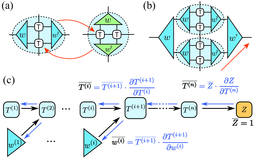
Figure 1: (Color online) (a) shows a TRG step where the scale transformations $w$ are introduced along both directions, while only vertical renormalization is involved in (b), which eventually compresses the tensor network into a 1D structure that can then be contracted exactly. (c) plots the computational graph of the forward TRG process as well as the backpropagation.

In the course of TRG process, environment of local tensors should be taken into account for conducting a precise truncation, through, e.g., isometric renormalization transformations in the tensor bases. This can be traced back to the renowned density matrix renormalization group White (1992), where the effects of environment are reflected in the reduced density matrix of “system" subblock. For generic tensor networks, second renormalization group (SRG) has been proposed to improve the process of tensor renormalization Xie et al. (2009); Zhao et al. (2010); Xie et al. (2012); Zhao et al. (2016). In SRG, the environment of local tensors is computed recursively, between different scales of a hierarchical network, with which a global optimization is feasible.

Recently, profound interplay between deep learning and tensor network algorithms has raised great interest Carleo and Troyer (2017); Carrasquilla and Melko (2017); van Nieuwenburg et al. (2017); Stoudenmire and Schwab (2016); Foreman et al. (2018); Han et al. (2018); Guo et al. (2018); Li and Wang (2018); Koch-Janusz and Ringel (2018). Among others, the differentiable programming is of particular interest for tensor networks. Given the computational graph generated in forward process, the gradient of corresponding variables can be calculated through the chain rule of derivatives in the backpropagation, with which the neural network can be deeply trained. The automatic calculation of gradients can be obtained within machine precision, and with same computational complexity of forward process. Very recently, this idea of differentiable programming that exploits a gradient based optimization, has been introduced to optimize tensor networks Liao et al. (2019).

In this work, we regard the renormalization transformation as input parameters of the TRG program, and point out that the SRG backward iteration bears a correspondence with the backpropagation algorithm in differentiable programming. Inspired by this substantial connection, we turn the idea of SRG into a generalized versatile framework, i.e., differentiable TRG ($\partial$TRG).

In $\partial$TRG, the forward TRG process is made fully differentiable, and the renormalization transformations are optimized globally and automatically through the backpropagation. We apply $\partial$TRG to simulate thermal equilibrium states at finite temperature, and achieve significantly improved accuracy over previous methods Li et al. (2011); Chen et al. (2018). The efficiency is demonstrated by implementing $\partial$TRG with PyTorch Paszke et al. ; pytorch , which facilitates the GPU computing and shows a high performance of about 40 times acceleration over a single CPU core.

Correspondence between SRG and backpropagation.— Backpropagation is a widely used method for training deep neural networks Rumelhart et al. (1986); Parker (1985); LeCun et al. (1989); Lecun et al. (2015), where the gradients of parameters can be computed through a reverse-mode automatic differentiation SM . On the other hand, SRG plays a very similar role in tensor-network algorithms as the backpropagation. To be specific, as shown in Figs. 1(a,c), a hierarchical tensor network can be constructed by piling up a series of isometric RG transformations $\left\{w^{(i)}\right\}$, with $i=1,2,...,n$ for each layer. In a well-designed TRG program, the input tensors $\left\{w^{(i)}\right\}$ are successively applied to the tensors $T$ and the output can be a tensor trace in general, e.g., partition function of a statistical system.

SRG takes the job to further optimize the renormalization transformations $\left\{w^{(i)}\right\}$ in the backward iteration, by making use of the environment. An adjoint tensor of $w^{(i)}$ at scale $i$ is defined as the gradient $\overline{w^{(i)}}$ ($\equiv\frac{\partial Z}{\partial w^{(i)}}$), which can be related to the environment through

$$E_{w}^{(i)}=\frac{1}{N_{i}}\overline{w^{(i)}},$$ (1)

where $N_{i}$ denotes the times $w^{(i)}$ appearing in the network, and $Z$ the tensor trace to be maximized. It directly follows from Eq. (1) that the recursive relations used in the backward iteration to determine $\left\{E^{(i)}\right\}$ in SRG, can be recasted into the derivative chain rule form, as depicted in Fig. 1(c). Remind that the multiplications there with Jacobians ${\partial T^{(i+1)}}/{\partial T^{(i)}}$ and ${\partial T^{(i+1)}}/{\partial w^{(i)}}$, etc, are conducted implicitly. They constitute sequences of tensor contractions exactly equivalent to the recursive tensor contractions in SRG SM .

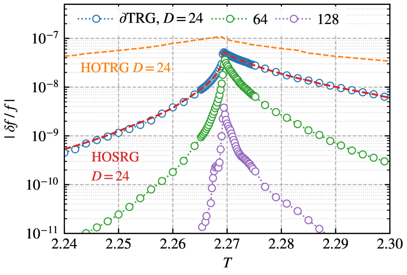
Figure 2: (Color online) The relative errors of free energy $|\delta f/f|$ in the vicinity of critical temperature $T_{c}$, obtained from HOTRG, HOSRG, and $\partial$TRG calculations. We perform $n_{i}=5$–10 iterations within each MERA update, and the total number of sweeps $n_{s}$ ranges from a few iterations to a few hundreds, depending on the specific temperature and scheme, until the relative errors reach a convergence criterion of $\epsilon=10^{-4}$. The $D=24$ $\partial$TRG calculations follows the scheme in Fig. 1(a), while $D=64$ and 128 cases the scheme in Fig. 1(b).

Differentiable tensor renormalization group.— Being aware of the intimate relation between the backpropagation and SRG, we now extend the latter to a more general and flexible framework, $\partial$TRG, with the help of well-developed automatic differentiation packages Wri , e.g., autograd autograd and PyTorch Paszke et al. ; pytorch . With these facilities, $\partial$TRG can record all operations performed on the input variables (tensors), and compute the derivatives [e.g. Eq. (1)] automatically in the backward iterations, with which the parameters $\left\{w^{(i)}\right\}$ can be optimized. Not limited within the original proposals Xie et al. (2009, 2012), the idea of SRG can be applied to various TRG schemes through the framework of differentiable programming. Below we consider two different $\partial$TRG schemes following the HOTRG Xie et al. (2012) and exponential TRG (XTRG) Chen et al. (2018), as shown in Figs. 1(a) and (b), respectively.

Once the environment $E_{w}^{(i)}$ is obtained, one can optimize $w^{(i)}$ with resorting to, e.g., standard quasi-Newton optimization method SM , or quasi-optimal schemes through tensor decompositions of $E_{w}^{(i)}$ Xie et al. (2009, 2012). Remind that a tensor decomposition scheme that keeps $w^{(i)}$ isometric has been developed in the context of multi-scale entanglement renormalization ansatz (MERA) algorithm Vidal (2007); Evenbly and Vidal (2009), which are mainly adopted in the simulations below. MERA update involves a singular value decomposition (SVD) $E_{w}=USV^{\dagger}$ and a replacement $w=UV^{\dagger}$, which maximizes the cost function $Z=$ Tr $(E_{w}\cdot w)$, with $O(D^{4})$ time complexity. Here $D$ is the geometric bond dimension of a tensor.

Due to the intrinsic nonlinearility (in $w$) in the optimization problem, $n_{i}$ inner iterations are introduced in a single step of MERA update ($n_{i}=5$–$10$ in practice). Moreover, thanks to the convenient access to $E_{w}^{(i)}$, in $\partial$TRG we can deeply optimize the tensor network via sweep optimizations. In practice, we scan from inner to outer layers $n_{s}$ times until the results converge, thus assuring a highly accurate global update of $\left\{w^{(i)}\right\}$ tensors.

$\partial$TRG of 2D Ising model.— As a first demonstration, we apply $\partial$TRG, with two specific implementations in Figs. 1(a,b), to solve the classical Ising model on the square lattice. Following the standard procedure, we can write down a square tensor-network representation consisted of rank-4 tensors $T$, whose TRG contraction results in the partition function $Z$ SM .

In Fig. 1(a), after $n$ steps of renormalizations, we obtain a single tensor representing the whole system of $2^{n}\times 2^{n}$ sites (in practice $n=25$ guarantees the thermodynamic limit), whose self-contraction leads to the partition function $Z$. On the other hand, after $n$ steps of renormalization, one arrives at an effective 1D system, whose complete contraction also leads to an accurate measure of the partition function.

In Fig. 2, we show the accuracies of $\partial$TRG implementations, together with the HOTRG and HOSRG data for comparisons. Owing to the sweep update, $\partial$TRG leads to errors clearly smaller than those of HOTRG, while achieving, as expected, the same accuracies as HOSRG footnote .

The two schemes of $\partial$TRG in Figs. 1(a) and (b) have different computational costs. The latter is considerably less resource-demanding, i.e., $O(D^{4})$ in computational time, while it is $O(D^{7})$ in Fig. 1(a). The memory costs are also dramatically different, i.e., $O(D^{5})$ for Fig. 1(a) and $O(D^{3})$ for (b). Therefore, we can push the $\partial$TRG simulations in Fig. 1(b) with bond states up to $D=128$, reaching much higher precision as shown in Fig. 2. From the comparison shown in Fig. 2, as well as other considerations, we chose the $\partial$TRG scheme in Fig. 1(b) to simulate quantum models as presented below.

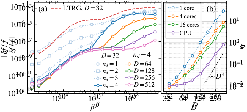
Figure 3: (Color online) (a) Comparisons of relative errors of free energy between linearized TRG (LTRG) and $\partial$TRG. In the initial $\rho(\tau)$ of $\partial$TRG, $\tau\simeq 5\times 10^{-5}$, which is also used as the Trotter slice in the LTRG calculations. The results are shown with optimization depth $n_{d}\leq 4$, $n_{i}=10$ in a single MERA update, and overall sweep iterations $n_{\rm{s}}=3$. (b) Comparisons of the computational walltime of $\partial$TRG on GPU and CPU with up to 16 cores, benchmarked on the infinite XY chain. The calculations are carried out on Nvidia Tesla V100 GPU and Intel Xeon 6230 CPU, with retained bond dimensions up to $D=360$. The dashed line depicts the scaling $t_{h}\sim D^{4}$.

Infinite quantum XY chain.— Now we employ $\partial$TRG to simulate the exactly solvable quantum XY chain

$$H_{XY}=\sum_{\langle i,j\rangle}S_{i}^{x}S_{j}^{x}+S_{i}^{y}S_{j}^{y}.$$ (2)

We start with preparing the density matrix $\rho(\tau)$ through (second order) Trotter-Suzuki decomposition SM . A very small imaginary-time step $\tau$ is chosen to ensure that Trotter errors are negligible. Given the matrix product operator (MPO) representation of $\rho(\tau)$, we proceed to cool down the system exponentially fast, with the $\partial$TRG algorithm shown in Fig. 1(b). The results are shown in Fig. 3(a), where the relative error $|\delta f/f|$ curves rise up from very small values at high temperature and increase monotonically as $T$ decreases.

In Fig. 3(a), benchmarking with the analytical solution Tu (2017); Chen et al. (2017a); SM , we compare the relative errors $|\delta f/f|$ between $\partial$TRG and LTRG, where the latter follows a cooling procedure linear in $\beta(\equiv 1/T)$ Li et al. (2011). It is observed that $\partial$TRG with depth $n_{d}=1$ (i.e., optimizing exclusively the current layer in the course of cooling) already outperforms LTRG in both efficiency and accuracy. By sweeping into $n_{d}$ (up to 4) layers, the accuracy is found to improve continuously in the relatively high to intermediate temperature regime due to better optimization. At low temperature, on the other hand, the enhancement of accuracy is marginal due to the limited expressibility of the tensor network with a given bond dimension $D=32$. Therefore, we show also in Fig. 3(a) the results of larger bond dimensions (up to 512), with a fixed depth $n_{d}=4$. There we observe that $|\delta f/f|$ decreases monotonically and attains very high accuracy, with relative error $\sim 10^{-7}$ at low temperature (down to $\beta\simeq 400$).

GPU acceleration.— We implement $\partial$TRG with the PyTorch library, and take advantage of GPU computing to significantly accelerate the simulations. In Fig. 3(b), we show the elapsed hours $t_{h}$ versus $D$ in the simulations of infinite XY chain on GPU and CPU, respectively. To quantify the speedup, $t_{h}$ is monitored at $\beta=12.8$, where the computation time falls well into a logarithmic scaling regime vs. $\beta$, i.e., $t_{h}\propto\ln{\beta}$ SM .

From Fig. 3(b), we observe approximately 40 times GPU acceleration (for $D=360$ calculations), as compared to single core CPU calculations, and over 7 times speedup to the 16-core parallel job. Moreover, in Fig. 3(b), the $t_{h}$ curves show algebraic scaling vs. $D$, i.e., $t_{h}\sim D^{\gamma}$, for sufficiently large $D$ where $\gamma$ values are found slightly less than 4. These appealing benchmarks, together with previous tests in Ref. Milsted et al. (2019), suggest that GPU acceleration indeed constitutes a very promising technique to be fully explored in quantum manybody computations, particularly in tensor network simulations.

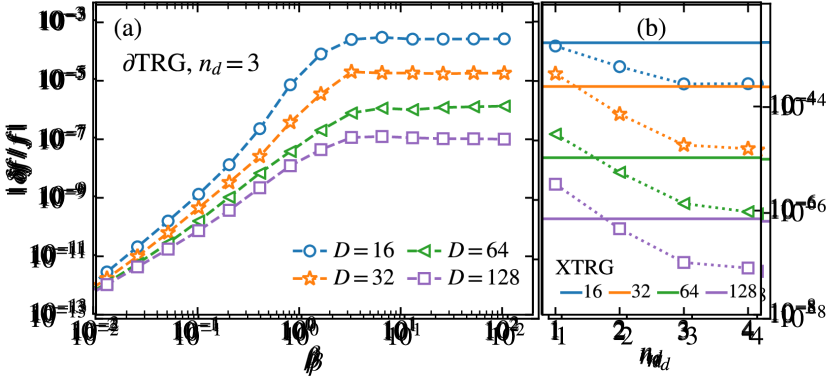
Figure 4: (Color online) (a) Relative errors of transverse-field Ising model on a $4\times 4$ open square lattice, at critical transverse field $h=h_{c}$. (b) $\partial$TRG results with various $D$ are plotted versus optimization depths $n_{d}=1,2,3$ and 4. The comparison is at a fixed low temperature $\beta\simeq 105$, and the standard XTRG results are shown with solid lines.

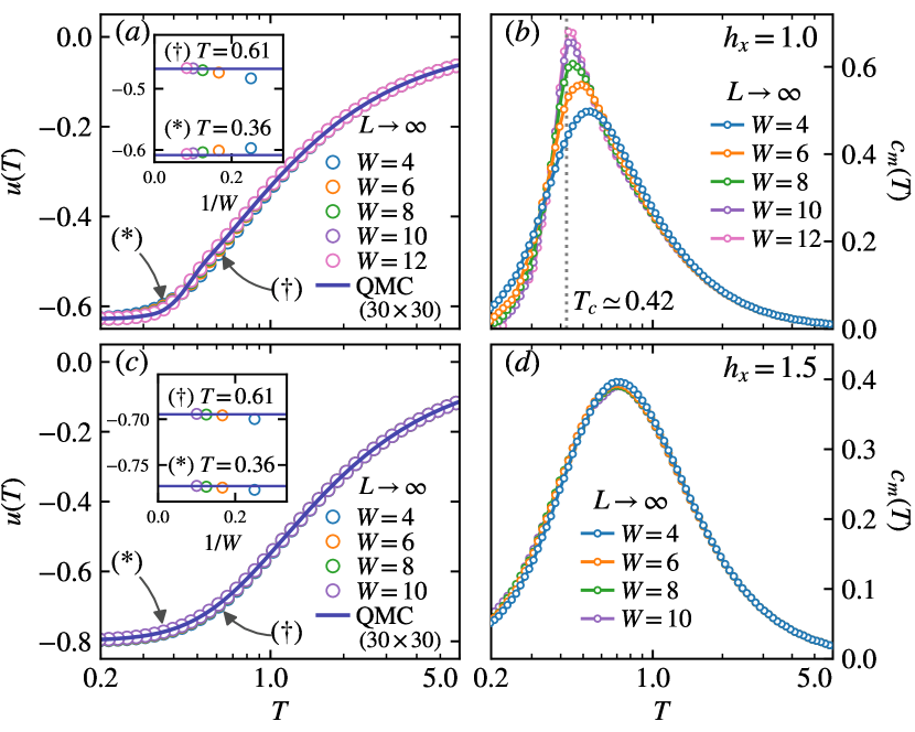
Figure 5: (Color online) The plot show internal energy $u(T)$ and spin specific heat $c_{m}(T)$ of transverse field Ising model, with $h_{x}=1$ [(a, b)] and $h_{x}=1.5$ [(c, d)]. $\partial$TRG calculations are run on cylinders of various widths $W$ (with length $L$ extrapolated to infinity). The energy data show excellent agreements with the quantum Monte Carlo (QMC) result Bauer et al. (2011) on a $30\times 30$ square lattice in both fields. For the $h_{x}=1$ case, the peak position in $c_{m}(T)$ provides an accurate estimate, $\sim 1$% relative error, of critical temperature.

Thermodynamics of finite-size quantum lattice models.— Now we apply $\partial$TRG to finite-size chains and cylindrical geometries of finite width $W$ (and length $L$), and try to approach the thermodynamics limit by increasing the system size, which has been proved to be very successful in ground-state simulations of quantum frustrated magnets White and Chernyshev (2007); He et al. (2017). Note that the sweep optimization needs to be adapted when applied to the finite-size systems, i.e., we not only scan $\left\{w^{(i)}\right\}$ between different scales but also among different lattice sites/bonds.

For a finite-size system on the 1D or 2D lattice, the high-$T$ density matrix $\rho(\tau)$ can be initialized through a discretization-error-free series expansion technique Chen et al. (2017b); SM . It has been shown to be preferable, over Trotter-Suzuki type initializations, in dealing 2D systems defined on, e.g., long cylinders Chen et al. (2018); Li et al. (2019). The benchmark results on the finite-size XY chain can be found in Supplementary Materials SM , where deep optimization into $n_{d}$ layers gains remarkable improvement in accuracy.

As a demonstration for 2D simulations, below we focus on the transverse-field Ising model on a square lattice, i.e.,

$$H=\sum_{\langle i,j\rangle}JS_{i}^{z}S_{j}^{z}-{h_{x}}\sum_{i}S_{i}^{x},$$ (3)

where $J=-1$ (ferromagnetic) is set as the energy scale. The model undergoes a magnetic order-disorder quantum phase transition at a critical field $h_{c}\simeq 1.52219(1)$ Blöte and Deng (2002). Through a snake-path mapping into quasi-1D lattice Li et al. (2019), the interaction information of the Hamiltonian Eq. (3) on a width $W$ cylinder can be encoded in a compact MPO of bond dimension $D_{H}=W+2$ Chen et al. (2018); Li et al. (2020). Given the MPO representation of $H$, $\partial$TRG works automatically and produces accurate results as benchmarked below.

Firstly, we run $\partial$TRG simulations on a 4$\times$4 square lattice at the critical transverse field $h=h_{c}$, and compare the results to exact diagonalization data. In Fig. 4(a), the relative errors $|\delta f/f|$ are plotted vs. $\beta$. One can observe a high accuracy with an optimization depth $n_{d}=3$, which continuously improves upon increasing the bond dimension $D$. Moreover, to reveal the effects of $n_{d}$, in Fig. 4(b) we show $|\delta f/f|$ vs. $n_{d}$ at low temperature, as compared to XTRG data. Indeed the accuracy improves considerably, by orders of magnitude, as $n_{d}$ increases. For example, the $D=64,n_{d}=4$ $\partial$TRG accuracy even goes parallel with the $D=128$ XTRG one.

Large-scale simulations and finite-temperature phase transition.— Next, we conduct $\partial$TRG calculations of quantum Ising model on cylinders with various widths $W$ (up to 12) and lengths $L$. The transverse field is first fixed at $h_{x}=1.0\approx 2/3h_{c}$, giving rise to a spin order in low temperature. The long-range order melts at a critical temperature $T_{c}\simeq 0.42$, through a second-order phase transition Czarnik and Dziarmaga (2015). In Fig. 5, we retain only moderate bond dimension up to $D=128$ in the calculations, and the optimization depth is up to $n_{d}=4$ layers. The internal energy $u(T)$ and magnetic specific heat $c_{m}(T)$ are computed from the first and second numerical derivatives of $f(T)$, respectively. Following the line developed in XTRG Chen et al. (2018); Li et al. (2019), we exploit a $z$-shift technique as well as numerical interpolation to collect dense enough data points and ensure a negligible differential error SM . Moreover, to eliminate the finite-length effects, we perform an extrapolation to $L=\infty$, via linear fitting or energy subtraction SM .

Collecting the extrapolated data at each width $W$, we compare the internal energy $u(T)$ with QMC data in Fig. 5(a). A very good agreement of our cylindrical results with the large-scale QMC data is obtained. The latter is computed on a $30\times 30$ square lattice with periodic boundary condition (i.e., torus) which mimics the thermodynamic limit. Furthermore, as shown in the inset, we zoom in at two selected temperatures and find there relative errors $|\delta u/u|\sim 10^{-3}$ ($W=12$ result), with respect to QMC. In Fig. 5(b), by further taking the derivatives of internal energy $u(T)$, we obtain the specific heat curves $c_{m}(T)$. It is observed that the peak in $c_{m}(T)$ gets sharper as $W$ increases, signaling the existence of a phase transition, and the peak locations for wide cylinders are in very good agreement with $T_{c}\simeq 0.42$ in the thermodynamic limit.

In Fig. 5(c,d), we provide $u(T)$ and $c_{m}(T)$ at transverse field $h_{x}=1.5\simeq 0.99h_{c}$, in close vicinity of the quantum phase transition point. Again, $u(T)$ results are in excellent agreement ($|\delta u/u|\sim 10^{-4}$) with the QMC data as shown in Fig. 5(c). It is observed in Fig. 5(d) that the specific heat shows a round peak at around $T/J=0.7$, which has well converged vs. system sizes and does not correspond to any phase transition, which should occur at below $T/J=0.2$.

Conclusion and outlook.— Inspired by the essential correspondence between the backpropagation and SRG of tensor networks, we propose the framework of $\partial$TRG. With $\partial$TRG, we make much better use of tensor parameters by increasing the optimization depth, instead of merely enlarging parameter space dimension $D$. As a result, a moderate $D$ can lead to an unprecedented high accuracy in simulating thermodynamics of 2D quantum models. Bearing the virtue of SRG, it can optimize both the wave function representation and the renormalization transformations, globally and automatically. Therefore, $\partial$TRG constitutes a promising tool to investigate very challenging manybody problems, e.g., frustrated antiferromagnets, fermionic Hubbard models, which are currently of great research interest.

Acknowledgments.— We are indebted to Jian Cui, Jan von Delft, Yannick Meurice, and Andreas Weichselbaum for helpful discussions. This work was supported by the National Natural Science Foundation of China (Grant Nos. 11774420, 11834014, 11974036, and 11774398), the National R$\&$D Program of China (Grants Nos. 2016YFA0300503, 2017YFA0302900), German Research Foundation (DFG WE4819/3-1) under Germany’s Excellence Strategy - EXC-2111 - 390814868 and by the Research Funds of Renmin University of China (Grants No. 20XNLG19). Our code implementation in PyTorch is publicly available at this https URL.

Supplemental Materials: Automatic Differentiation for Second Renormalization of Tensor Networks

A Tensor network representation of the Ising model and its renormalization

In this section, we briefly discuss some basic notions on the real-space tensor renormalization group (TRG) methods, which was referred to as rewiring method in literatures, e.g., Ref. Efrati et al. (2014). For the sake of simplicity, we take the Ising model on the square lattice as an example. Due to the locality of the interaction, the partition function has a compact tensor-network representation Zhao et al. (2010), i.e.,

$$Z=\sum_{\{\sigma\}}e^{-\beta H(\{\sigma\})}=\sum_{\{\sigma\}}\prod_{a}T_{\sigma_{i}\sigma_{j}\sigma_{k}\sigma_{l}}^{(a)}$$ (A1)

where $\{\sigma\}$ denotes the classical spin configurations in the Hamiltonian $H$. The tensor $T^{(a)}$ is defined on a local plaquette, labeled as $a$, containing the four original spins. The central idea of renormalization group lies in the concept of renormalization transformation Wilson (1975); Kadanoff (1975), in which a set of new coupling constants $\{K\}$ is sought to represent the Hamiltonian as

$$H=\sum_{a,i}K_{i}s^{(a)}_{i},$$ (A2)

where $s^{(a)}_{i}$ defined at a larger scale is a “block spin", i.e., combination of original spins $\{\sigma\}$ in the plaquette $a$.

Accordingly, in the rewiring method, TRG finds a set of tensors $\{T^{(a^{\prime})}\}$ defined at plaquette $a^{\prime}$ (thus at a larger length scale) to represent the partition function, i.e.,

$$Z=\sum_{\{\alpha\}}\prod_{a^{\prime}}T_{\alpha_{i}\alpha_{j}\alpha_{k}\alpha_{l}}^{(a^{\prime})},$$

where the tensors $T$ are obtained following a similar line of Kadanoff’s RG transformation: We introduce new statistical variables $\{\alpha\}$ (as geometric indices of tensors) and then trace out the original variables $\{\sigma\}$. TRG methods provide accurate tool and versatile platform for studying the conformal criticality and universality near phase transition temperatures Efrati et al. (2014).

In TRG, the transformations between $T_{\sigma_{i}\sigma_{j}\sigma_{k}\sigma_{l}}$ at small length scale and $S_{\alpha_{i}\alpha_{j}\alpha_{k}\alpha_{l}}$ at a larger one constitute the most important parameters of the program. Once the transformations are given, they renormalize the system and result in the partition function $Z$. In most cases, approximations have to be introduced in the course of TRG, while causing minimal loss in the partition function. We point out that, while most TRG programs employs renormalization transformations that are found only locally Levin and Nave (2007); Gu and Wen (2009); Evenbly and Vidal (2015a); Yang et al. (2017); Bal et al. (2017), the second renormalization group (SRG) Xie et al. (2009); Zhao et al. (2010); Xie et al. (2012); Zhao et al. (2016) manages to find proper transformations that optimizes the partition function globally.

B Second renormalization group

In the following, we recapitulate SRG in the higher-order tensor renormalization group (HOTRG) algorithm, i.e., HOSRG Xie et al. (2012); Zhao et al. (2016). For a lattice system with translational invariance, $T^{(i)}$ is used to denote the local tensors renormalized at the $i$-th scale. $i=1$ denotes the initial scale at which the original Hamiltonian is defined, and $w^{(i)}$ is the $i$-th isometric renormalization transformation. As shown in Fig. S1, given the renormalization transformations, we can perform a forward HOTRG iteration,

$$T^{(i+1)}_{\alpha\beta yy^{\prime}}=\sum_{jx_{1}x_{2}x^{\prime}_{1}x^{\prime}_{2}}T^{(i)}_{x_{1}x^{\prime}_{1}yj}T^{(i)}_{x_{2}x^{\prime}_{2}jy^{\prime}}w^{(i)}_{x_{1}x_{2}\alpha}w^{(i)}_{x^{\prime}_{1}x^{\prime}_{2}\beta}$$ (B3)

where the subscripts ${x_{1},x_{2},\alpha}$ of $w_{x_{1}x_{2}\alpha}^{(i)}$ can be understood as the new statistical variables introduced at different scales, with which the Hamiltonian can be written down, c.f., Eq. (A2). The transformations $w^{(i)}$ between two scales $i$ and $i+1$ are determined by the local higher-order singular value decompositions according to tensors $T^{(i)}$.

Figure S1: Illustration of forward process in Eq. (B3). Note that in the backward recursive equation Eq. (B4), the upper $T^{(i)}$ is denoted as $T^{(i;u)}$, and the lower one $T^{(i;d)}$.

In the forward HOTRG iteration described above, the transformations $w^{(i)}$ is determined locally Xie et al. (2012). To achieve a global optimization, the environment tensor $E$ should be considered. We punch a “hole” by removing the target tensor in the tensor network and contract all the indices except those of the target. A backward iteration should be involved to accomplish this task and perform the global optimization.

For example, the environment of $T^{(i)}$ at the target scale $i$ can be obtained exploiting the following recursive relation

$$E^{(i;u)}_{x_{1}x^{\prime}_{1}yj}=\sum_{\alpha\beta y^{\prime}x_{2}x^{\prime}_{2}}E^{(i+1)}_{\alpha\beta yy^{\prime}}T^{(i;d)}_{x_{2}x^{\prime}_{2}jy^{\prime}}w^{(i)}_{x_{1}x_{2}\alpha}w^{(i)}_{x^{\prime}_{1}x^{\prime}_{2}\beta}$$ (B4)

where the superscripts $\lambda=\left(u,d\right)$ denote the upper and lower $T^{(i)}$ in Fig. S1, and environment $E^{(i)}$ is averaged over two equivalent environment, i.e., $E^{(i)}=\sum_{\lambda}E^{(i;\lambda)}/2$, with $\lambda=u,d$. Given the environment tensor $E^{(i)}$, we can update the renormalization transformation $w^{(i)}$ that globally optimizes the partition function.

C Backpropagation in neural networks

Generally speaking, a deep feedforward neural network sets up a mapping between a set of input signals $x^{(1)}$, such as images, and a set of output signals $y$, say, categories, through a multi-layer transformation $\mathcal{F}$, i.e., $y=\mathcal{F}(x^{(1)})$, where $\mathcal{F}$ is represented as a composition of many arranged linear ($\mathcal{L}$) transformations separated by nonlinear ($\mathcal{N}$) mappings. To be specific, an $n$-layer neural network $\mathcal{F}$ can be expressed as

$$\mathcal{F}=\mathcal{N}^{(n)}\mathcal{L}^{(n)}...\mathcal{N}^{(2)}\mathcal{L}^{(2)}\mathcal{N}^{(1)}\mathcal{L}^{(1)}$$ (C5)

where the linear transformations $\mathcal{L}$’s contain most of the variational parameters $\omega$’s that need to be optimized. Roughly speaking, the major goal of training a neural network is to find the optimal $\omega$’s which minimize the target objective function $L$ characterizing the discrepancy between the actual and predicted labels.

In essence, each layer of the neural network, i.e., $\mathcal{L}^{(i)}$ followed by $\mathcal{N}^{(i)}$, perform the transformations on the input data/feature $x^{(i)}$, and its output $x^{(i+1)}$ can be regarded as a new representation and a higher-level abstraction of original input Li and Wang (2018); Koch-Janusz and Ringel (2018). This is very similar to the renormalization transformation of TRG described in the main text, where new bases are introduced in different scales to represent the original partition function.

To train the neural network, the gradients of the objective function $L$ with respect to the parameters $\omega$’s are required for a global optimization. The backpropagation algorithm, arguably the most successful approach for training deep neural networks, exploits the chain rule of derivatives to efficiently compute these gradients Rumelhart et al. (1986); Parker (1985); LeCun et al. (1989); Lecun et al. (2015). To be concrete, the backpropagation method relates the gradients in two neighboring layers as follows

$$\frac{\partial{L}}{\partial{x^{(i)}}}=\frac{\partial{L}}{\partial{x^{(i+1)}}}\cdot\frac{\partial{x^{(i+1)}}}{\partial{x^{(i)}}}.$$ (C6)

In deep learning, automatic differentiation (AD) technique is employed to compute the derivative $\frac{\partial{L}}{\partial{x^{(i)}}}$ following the recursive equation Eq. (C6), in an analytically rigorous way. Furthermore, the derivatives with respect to the parameters $\omega^{(i-1)}$ can be similarly obtained via one more AD step through $\frac{\partial{x^{(i)}}}{\partial{\omega^{(i-1)}}}$, with which one can update $\omega^{(i-1)}$ and regenerate $x^{(i)}$ in the $i$-th layer.

D Quasi-Newton optimization of isometries

Given the gradient $E_{w}^{(i)}=\frac{1}{N_{i}}\overline{w^{(i)}}$ [see Eq. (1) in the main text], the quasi-Newton approach constitutes a class of efficient algorithm for parameter optimization. Here in $\partial$TRG, to impose the isometric constraint, we choose the parametrization $w^{(i)}=\exp{\left(B^{(i)}\right)}$, where $B^{(i)}$ is an anti-symmetric real square matrix of dimension $D^{2}$.

With this parameterization, the standard gradient based L-BFGS method Wri can be employed to update $B^{(i)}$ so as to maximize $Z$. After an exponential operation, we can then compute $\exp{\left(B^{(i)}\right)}$ numerically and then truncate this unitary matrix (of dimension $D^{2}$, see main text) into a $D^{2}\times D$ isometry $w^{(i)}$.

Note the computational cost of this “tailored" quasi-Newton approach is of time complexity $O(D^{6})$, higher than the MERA update $O(D^{4})$ that we used in the main text.

E Details on the correspondence between SRG and backpropagation

Suppose the tensor elements in $w^{(i)}$s are independent variational parameters, we can bridge SRG and backpropagation approach, in the context of higher-order tensor renormalizations, by comparing Eq. (B4) and Eq. (C6).

From SRG to backpropagation: Firstly, we assert the following formula which equals “punching a hole" in the tensor network to the derivative

$$E^{(i;\lambda)}_{abcd} = \frac{1}{N_{i}}\cdot\frac{\partial{Z}}{\partial{T^{(i;\lambda)}_{abcd}}}=\frac{\sum_{j}E^{(i,j;\lambda)}_{abcd}}{N_{i}},$$ (E7)

where $2N_{i}=2^{(n-i+1)}$ is the number of $T^{(i)}$ copies (labeled by index $j$) in the partition function tensor network, i.e., $Z=\mathrm{Tr}\left(T^{(i)}\right)^{\otimes 2N_{i}}$. Matter of fact, the equation

$$Z=\sum_{abcd}T^{(i,j;\lambda)}_{abcd}E^{(i,j;\lambda)}_{abcd}$$

holds at all scales $i$ and location $j$. Next, we point out that the tensor contractions in Eq. (B4) is nothing but multiplying Jacobian to the tensor $E^{(i+1)}$, i.e.,

$$\frac{\partial{T^{(i+1)}_{\alpha\beta yy^{\prime}}}}{\partial{T^{(i;u)}_{x_{1}x^{\prime}_{1}zj}}} = \delta_{yz}\cdot\sum_{x_{2}x^{\prime}_{2}}T^{(i;d)}_{x_{2}x^{\prime}_{2}jy^{\prime}}w^{(i)}_{x_{1}x_{2}\alpha}w^{(i)}_{x^{\prime}_{1}x^{\prime}_{2}\beta},$$ (E8)

which is the derivative of $T^{(i+1)}$ with respect to $T^{(i;u/d)}$, self-evident in Fig. S1. Combining Eq. (E7) and Eq. (E8) together, we can rewritten Eq. (B4) as

$$\frac{\partial{Z}}{\partial{T^{(i)}_{abcd}}} = \sum_{xyzw}\frac{\partial{Z}}{\partial{T^{(i+1)}_{xyzw}}}\cdot\frac{\partial{T^{(i+1)}_{xyzw}}}{\partial{T^{(i)}_{abcd}}}$$ (E9)

where $\frac{\partial{T^{(i+1)}}}{\partial{T^{(i)}}}=\sum_{\lambda}\frac{\partial{T^{(i+1)}}}{\partial{T^{(i;\lambda)}}}$ is assumed.

Therefore, we reach the conclusion that the recursive relation of environment in the SRG backward iteration, as expressed in Eq. (B4), is exactly the derivative chain rule Eq. (C6) in backpropagation method of deep learning. In Eq. (E9), we have customized the backpropogation with the tensor network context to emphasize the in-depth link between the two.

Moreover, to show the correspondence in a more intuitive way, we introduce the following notations

(E10)

and represent the Jacobian $\frac{\partial{T^{(i+1)}}}{\partial{T^{(i)}}}$ in Eq. (E8) as

$$\leavevmode\hbox to55.26pt{\vbox to62.18pt{\text{[drawing]}}}\hskip 5.0pt+\hskip 5.0pt\leavevmode\hbox to55.26pt{\vbox to64.82pt{\text{[drawing]}}}\hskip 5.0pt\doteq\hskip 5.0pt\frac{\partial{T^{(i+1)}_{xyzw}}}{\partial{T^{(i)}_{abcd}}}. x y z=c w a b d x y z w=d a b c x y z=c w a b d x y z w=d a b c$$ (E11)

Then we can picturize Eq. (E9) as

$$= \frac{1}{2}\times\left[\leavevmode\hbox to55.26pt{\vbox to41.03pt{\text{[drawing]}}}\hskip 5.0pt+\hskip 5.0pt\leavevmode\hbox to55.26pt{\vbox to41.03pt{\text{[drawing]}}}\right]$$

$$= \frac{1}{2}\times\leavevmode\hbox to23.96pt{\vbox to23.96pt{\text{[drawing]}}}\times\left[\leavevmode\hbox to55.26pt{\vbox to41.03pt{\text{[drawing]}}}\hskip 5.0pt+\hskip 5.0pt\leavevmode\hbox to55.26pt{\vbox to41.03pt{\text{[drawing]}}}\right]$$

where the open indices represent identities, same as those in Eq. (E10) and Eq. (E11).

From backpropagation to SRG: Now we start from Eq. (E9) and try to recover the SRG operation. Given that the tensor network derivative equals environment tensor $E^{(i)}$ (up to a factor), the key step in backpropagation approach is also the computing of Jacobian ${\partial T^{(i+1)}}/{\partial T^{i}}$. In AD technique, this is implicitly expressed as a sequence of tensor contractions exactly reverse the forward process, as also shown in Eq. (E11) (while from right hand side to left). That is to say, the Jacobian is computed in AD by contracting $T^{(i;d)}_{x_{2}x^{\prime}_{2}jy^{\prime}},w^{(i)}_{x_{1}x_{2}\alpha},w^{(i)}_{x^{\prime}_{1}x^{\prime}_{2}\beta}$ with the derivative ${\partial Z}/{\partial T^{(i+1)}}=N_{i+1}E^{(i+1)}$ from the $(i+1)$-th layer. Therefore, we again arrive at Eq. (LABEL:Note3) and confirm that the recursive relation used in SRG is equivalent to the chain-rule AD procedure in backpropagation.

F Initialization of $\rho(\tau)$

In the simulation of quantum lattice models, we start from high temperature density operator $\rho(\tau)$, with a given manybody Hamiltonian $H$. There are two ways preparing $\rho(\tau)$ and obtaining its matrix product operator (MPO) representation. For infinite 1D quantum chains, we can employ a Trotter-Suzuki decomposition of $\rho(\tau)=e^{-\tau H}$, while for an finite-size system the series expansion technique offers us a discretization-error-free approach to prepare the MPO $\rho(\tau)$. Given the initial $\rho(\tau)$, we can perform successively the exponential cooling procedure down to the require low temperature.

To perform the Trotter-Suzuki decomposition, we rewrite the Hamiltonian

$$H_{XY}=\sum_{i}h_{i,i+1}=\sum_{i}S_{i}^{x}S_{i+1}^{x}+S_{i}^{y}S_{i+1}^{y},$$ (F13)

as

$$H_{XY}=H_{o}+H_{e},$$

where $H_{o(e)}=\sum_{i\in odd(even)}h_{i,i+1}$ contains odd(even) terms. Therefore, up to $O(\tau^{3})$ Trotter error, $e^{-\tau H_{XY}}=e^{-\frac{\tau}{2}H_{o}}e^{-\tau H_{e}}e^{-\frac{\tau}{2}H_{o}}$. With sufficiently small $\tau$, e.g., $\tau\simeq 5\times 10^{-5}$ in Fig. 3 of the main text, the Trotter error has been very well-controlled in practice.

On the other hand, for finite-size systems, including 2D systems mapped into quasi-1D chains with “long-range" interactions, we employ the series expansion of the density matrix

$$e^{-\tau H}=\sum_{n=1}^{N_{c}}\frac{(-\tau)^{n}}{n!}H^{n},$$ (F14)

to realize an initialization of $\rho(\tau)$. By retaining sufficient large $N_{c}$, Eq. (F14) is free of any essential expansion error. Therefore, given an MPO representation of $H$, the density matrix $\rho(\tau)$ can be computed via the series-expansion machinery Chen et al. (2017b), for both 1D and 2D finite-size systems.

Given the MPO representation of initial $\rho_{0}(\tau)$ at high temperature, the system can be cooled down linearly (LTRG) Li et al. (2011) or exponentially (XTRG) Czarnik and Dziarmaga (2015); Chen et al. (2018) along the $\beta$ axis. Due to the much fewer truncation steps, it has been shown that XTRG constitutes a more accurate way of thermodynamic simulations Chen et al. (2018, 2019); Li et al. (2019) and is thus adopted in the current work of $\partial$TRG.

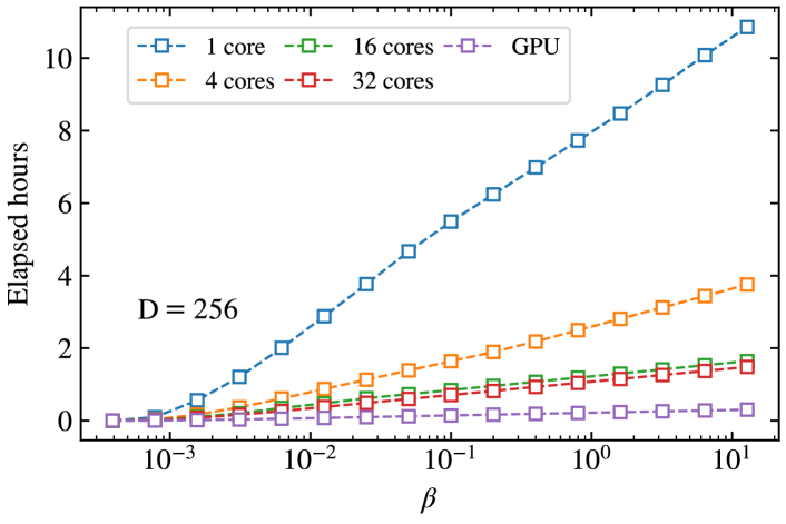
Figure S2: (Color online) Elapsed hours $t_{h}$ scaling versus $\beta$, where a logarithmic scaling, i.e., $t_{h}\sim\ln{\beta}$ can be seen in both GPU and CPU (1, 4, and 16 cores) runs.

G Exact solution of quantum XY chain at finite temperature

We hereby provide the exact expression of partition function for 1-D quantum XY chain,

$$H=J\sum_{i=1}^{N}\left(S^{x}_{i}S^{x}_{i+1}+S^{y}_{i}S^{y}_{i+1}\right)=\frac{J}{2}\sum_{i=1}^{N}\left(S^{+}_{i}S^{-}_{i+1}+S^{-}_{i}S^{+}_{i+1}\right)$$ (G15)

with the periodic boundary condition $S^{\pm}_{N+1}=S^{\pm}_{1}$. Exploiting the Jordan-Wigner transformation

$$\begin{cases}S^{+}_{j}&=e^{-i\pi\sum_{k<j}c^{\dagger}_{k}c_{k}}c_{j}^{\dagger},\\ S^{-}_{j}&=e^{i\pi\sum_{k<j}c^{\dagger}_{k}c_{k}}c_{j}^{\dagger},\\ S^{z}_{j}&=c_{j}^{\dagger}c_{j}-\frac{1}{2},\end{cases}$$ (G16)

the Hamiltonian can be expressed as a spinless fermionic tight-binding chain,

$$H=\frac{J}{2}\left(\sum_{i=1}^{N-1}c^{\dagger}_{i}c_{i+1}-Qc^{\dagger}_{N}c_{1}\right)+h.c.$$ (G17)

with the parity $Q\equiv e^{-i\pi\sum_{j=1}^{N}c^{\dagger}_{j}c_{j}}$ being a conserved quantity. The Hilbert space then splits into two independent sectors: $Q=1$ (even particle number) sector; $Q=-1$, (odd particle number )sector, and the Hamiltonian can be expressed as,

$$H=\frac{J}{2}\sum_{i=1}^{N}c^{\dagger}_{i}c_{i+1}+h.c.,$$ (G18)

with periodic(anti-periodic) boundary condition $c_{N+1}=\pm c_{1}$ in even(odd) sector. Through Fourier transformation $c_{j}=1/\sqrt{N}\sum_{q}e^{-iqj}c_{q}$, the Hamiltonian gets diagonalized into,

$$H=J\sum_{q}\cos{(q)}~{}c_{q}^{\dagger}c_{q}=\sum_{q}\epsilon_{q}~{}c_{q}^{\dagger}c_{q},$$ (G19)

where $k$’s are summed over modes $q=q_{+}\equiv 2\pi n/N$ in even sector while over $q=q_{-}\equiv 2\pi(n+1/2)/N$ in odd sector, with $n=0,1,\cdots,(N-1)$, to cope with corresponding boundary conditions.

With even particle number constraint in $Q=1$ sector, the many-body states with odd numbers of modes should be excluded, when calculating the partition function Chen et al. (2017a); Tu (2017). Thus, the partition function $Z_{+}$ in even sector is,

$$Z_{+}(\beta)=\frac{1}{2}\prod_{q_{+}}(1+e^{-\beta\epsilon_{q_{+}}})+\frac{1}{2}\prod_{q_{+}}(1-e^{-\beta\epsilon_{q_{+}}}).$$ (G20)

Similarly, the many-body states with even numbers of modes occupied should be excluded in $Q=-1$ sector, and the partition function reads as,

$$Z_{-}(\beta)=\frac{1}{2}\prod_{q_{-}}(1+e^{-\beta\epsilon_{q_{-}}})-\frac{1}{2}\prod_{q_{-}}(1-e^{-\beta\epsilon_{q_{-}}}).$$ (G21)

Finally, one arrives at the partition function in the entire Hilbert space as,

$$Z=Z_{+}+Z_{-},$$ (G22)

from which one can calculate the free energy and other thermodynamic quantities.

H XY chain: computational hours $t_{h}$ versus $\beta$

Here we provide the elapsed real time $t_{h}$ vs. $\beta$ in simulating the infinite XY chain. In Fig. S2, we show the $D=256$ runs with various numbers of CPU cores (Xeon Gold 6230) as well as on the GPU (Tesla V100). We can see clearly a logarithmic scaling between $t_{h}$ and $\beta$, for $\beta\gtrsim 0.1$. This logarithmic instead of linear scaling of wall time $t_{h}$ vs. $\beta$ clearly indicates the exponential speed up in $\partial$TRG. In addition, from Fig. S2 we can see that in all cases (either GPU or CPU computations with various cores) $\beta=12.8$, the temperature point we have selected in Fig. 3(b) of the main text, is located well in the logarithmic regime. That is to say, it constitutes a well suitable sampling temperature point for checking the $t_{h}$ vs. $D$ scaling in Fig. 3(b).

I $\partial$TRG calculations of finite-size XY chain

Due to the absence of translational invariance in finite-size systems, when applying $\partial$TRG to such systems, the isometries $w$ are bond dependent. Therefore, extra care is required in the optimization of $w$ tensors, as will be elaborated below.

Following that introduced in Sec. F, we prepare the matrix product operator (MPO) representation of $\rho(\tau)$ via the series expansion. After the initialization, similar to the infinite cases, one perform iteratively renormalization of tensors to cool down the system from high to low temperatures, and can also sweep into inner $n_{d}$ layers. Nevertheless, there exist in finite-size $\partial$TRG algorithms bond-dependent isometries to be optimized, thus sweeps amongst different bonds are required, along with those between different temperature scales.

The finite-size XY spin chain can be solved exactly by a Jordan-Wigner transformation that maps the system into a non-interacting spinless fermion chain, from which the partition function can be readily obtained Chen et al. (2018). In Fig. S3, we perform the calculation of an $L=50$ XY chain and show the relative errors of free energy for various dimensions $D$ (up to $D=128$) and depths $n_{d}$ (up to 3). Similar to the observations for infinite-size chain shown in Fig. 3 of the main text, we can see in Fig. S3 the accuracy improves significantly as the sweep depth $n_{d}$ increases. Moreover, as shown in Fig. S3, the improvement gets more and more pronounced as $D$ increases from $D=32$ to 128. In particular, the improvement of accuracies gains over a wide range of temperatures, i.e., from high down to low temperatures. This again reveals unambiguously the advantage of deep optimization in $\partial$TRG.

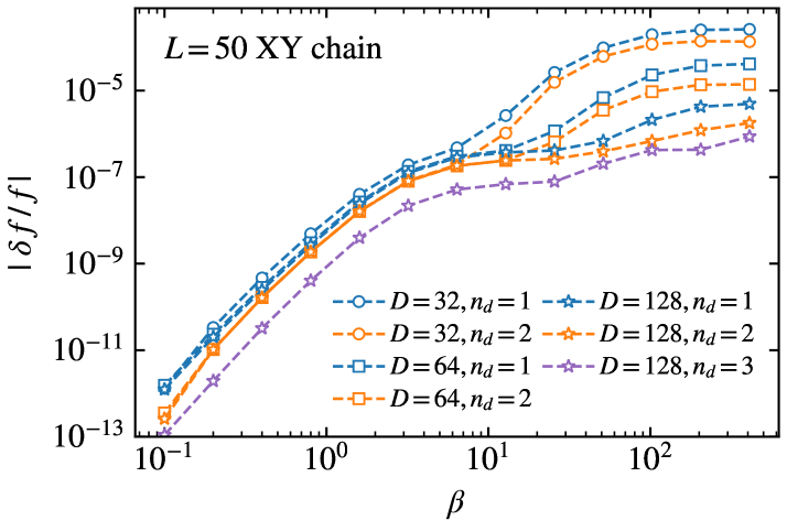
Figure S3: (Color online) Relative errors of free energy $|\delta f/f|$ in $L=50$ quantum XY chain computed by $\partial$TRG. There is continuous improvement in the accuracies with the increase of bond dimensions $D=32,64$, and $128$, as well as the sweep depths $n_{d}=1,2$, and $3$.

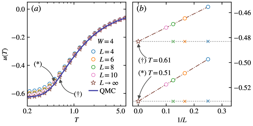
Figure S4: (Color online) (a) Internal energy $u(T)$ of TFI in field $h_{x}=1.0$ with fixed cylinder width $W=4$ and various $L$ (up to 10), which is used to extrapolate to $L=\infty$. It is benchmarked by QMC data with $W=4,L=\infty$ with similar extrapolations performed. (b) demonstrates the extrapolations through both the linear fitting and the subtraction technique (depicted as the cross marks), where excellent agreement is seen between the two schemes. The dotted horizontal line goes strictly through the extrapolated values (the star symbols), which is in perfect agreement with the subtraction results $u_{sub}$ (cross marks).

J The $z$-shift technique

In this appendix, we will briefly recapitulate the $z$-shift technique for the computation of thermodynamic quantities in $\partial$TRG. Below we take the internal energy $u$ as an example, which is obtained by taking numerical derivative of free energy $f$, i.e.,

$$u\equiv\frac{\partial{(\beta f)}}{\partial{\beta}}=\frac{\partial{(\beta f)}}{\partial{\ln\beta}}\cdot\frac{1}{\beta}$$ (J23)

as adopted in previous XTRG simulations Chen et al. (2018, 2019); Li et al. (2019). In the case of the temperature grid denoted as

$$\{\beta_{i}\}\equiv\{2^{i}\cdot\tau_{0}\}=\{\tau_{0},~{}2\tau_{0},~{}4\tau_{0},~{}...,~{}2^{n}\tau_{0}\}$$

being sparse, one can resort to the $z$-shift technique by shifting the initial temperature $\tau$ by a $z$-factor

$$\tau=z\cdot\tau_{0},\quad\mathrm{with}~{}z\in[1,2),$$ (J24)

and thus obtain a new grid

$$\{z\cdot\beta_{i}\}\equiv\{2^{i}\cdot\tau\}=\{\tau,~{}2\tau,~{}4\tau,~{}...,~{}2^{n}\tau\}.$$

Note that following the new grid $\{z\cdot\beta_{i}\}$ the simulations can be performed in parallel to the original $\{\beta_{i}\}$ run, thus constituting a highly efficient approach in XTRG Chen et al. (2018) as well as $\partial$TRG.

To be specific, as shown in Fig. 5 of main text, we conduct the $\partial$TRG simulations by following 4 sets of temperature grids $\{z\cdot\beta_{i}\}$ with $z$-factor chosen to be $z=2^{0},2^{\nicefrac{{1}}{{4}}},2^{\nicefrac{{1}}{{2}}},2^{\nicefrac{{3}}{{4}}}$. Before taking the numerical derivative Eq. (J23), in practice we further employ an interpolation of free energy data to reach an even denser temperature grid, i.e., totally 16 sets with $z=2^{0},2^{\nicefrac{{1}}{{16}}},...,2^{\nicefrac{{15}}{{16}}}$, which turns out to essentially eliminate the differential errors.

K Energy extrapolations of 2D transverse-field Ising model

In this section, we demonstrate the extrapolations of internal energy $u(T)$ in transverse-field Ising (TFI) model on the cylindrical square lattice, via both linear fitting and subtraction methods, as mentioned in the main text. In Fig. S4(a), we show the internal energy in a $W=4$ TFI model with various length $L=4,6,8,10$. To some extent, they already show nice convergence with each other as well as to the large-scale QMC data. Nonetheless, one can still extrapolate further to $L=\infty$ limit to eliminate the small finite-length effects, by either linear fitting $u_{L}=u_{\infty}+b/L$ or energy subtractions, i.e., $e_{sub}=(e_{L+2}-e_{L})/2W$ representing the ‘bulk’ energy. As shown in Fig. S4(b), both schemes generate mutually consistent energies in the $L=\infty$ limit, as indicated by the horizontal grey dotted lines which goes through exactly the extrapolated value [the asterisk symbol in Fig. S4(b)]. Remind that the subtracted energy values get converged much faster to the infinite length limit than linear extrapolation and thus constitutes a more efficient technique in practice for extracting bulk energy expectation values.

References

Levin and Nave (2007)M. Levin and C. P. Nave, “Tensor
renormalization group approach to two-dimensional classical lattice
models,” Phys. Rev. Lett. 99, 120601 (2007).
Gu and Wen (2009)Z.-C. Gu and X.-G. Wen, “Tensor-entanglement-filtering renormalization approach and
symmetry-protected topological order,” Phys.
Rev. B 80, 155131
(2009).
Xie et al. (2012)Z. Y. Xie, J. Chen, M. P. Qin, J. W. Zhu, L. P. Yang, and T. Xiang, “Coarse-graining renormalization by higher-order singular value
decomposition,” Phys. Rev. B 86, 045139 (2012).
Evenbly and Vidal (2015b)G. Evenbly and G. Vidal, “Tensor network
renormalization yields the multiscale entanglement renormalization ansatz,” Phys. Rev. Lett. 115, 200401 (2015b).
Yang et al. (2017)S. Yang, Z.-C. Gu, and X.-G. Wen, “Loop optimization for tensor network
renormalization,” Phys. Rev. Lett. 118, 110504 (2017).
Bal et al. (2017)M. Bal, M. Mariën,
J. Haegeman, and F. Verstraete, “Renormalization group flows of
Hamiltonians using tensor networks,” Phys. Rev. Lett. 118, 250602 (2017).
Jiang et al. (2008)H. C. Jiang, Z. Y. Weng, and T. Xiang, “Accurate determination of tensor
network state of quantum lattice models in two dimensions,” Phys. Rev. Lett. 101, 090603 (2008).
Li et al. (2011)W. Li, S.-J. Ran,
S.-S. Gong, Y. Zhao, B. Xi, F. Ye, and G. Su, “Linearized tensor renormalization group algorithm for the calculation of
thermodynamic properties of quantum lattice models,” Phys. Rev. Lett. 106, 127202 (2011).
Czarnik et al. (2012)P. Czarnik, L. Cincio, and J. Dziarmaga, “Projected entangled pair
states at finite temperature: Imaginary time evolution with ancillas,” Phys. Rev. B 86, 245101 (2012).
Dong et al. (2017)Y.-L. Dong, L. Chen, Y.-J. Liu, and W. Li, “Bilayer linearized tensor renormalization group
approach for thermal tensor networks,” Phys.
Rev. B 95, 144428
(2017).
Kshetrimayum et al. (2019)A. Kshetrimayum, M. Rizzi,
J. Eisert, and R. Orús, “Tensor network annealing algorithm for
two-dimensional thermal states,” Phys. Rev. Lett. 122, 070502 (2019).
Czarnik and Dziarmaga (2015)P. Czarnik and J. Dziarmaga, “Variational
approach to projected entangled pair states at finite temperature,” Phys. Rev. B 92, 035152 (2015).
Corboz et al. (2018)P. Corboz, P. Czarnik,
G. Kapteijns, and L. Tagliacozzo, “Finite correlation length
scaling with infinite projected entangled-pair states,” Phys.
Rev. X 8, 031031
(2018).
Czarnik and Corboz (2019)P. Czarnik and P. Corboz, “Finite
correlation length scaling with infinite projected entangled pair states at
finite temperature,” Phys. Rev. B 99, 245107 (2019).
Chen et al. (2018)B.-B. Chen, L. Chen, Z. Chen, W. Li, and A. Weichselbaum, “Exponential thermal tensor network approach for
quantum lattice models,” Phys. Rev. X 8, 031082 (2018).
Li et al. (2019)H. Li, B.-B. Chen,
Z. Chen, J. von Delft, A. Weichselbaum, and W. Li, “Thermal tensor renormalization group simulations of
square-lattice quantum spin models,” Phys. Rev. B 100, 045110 (2019).
Xie et al. (2009)Z. Y. Xie, H. C. Jiang,
Q. N. Chen, Z. Y. Weng, and T. Xiang, “Second renormalization of tensor-network
states,” Phys. Rev. Lett. 103, 160601 (2009).
Zhao et al. (2010)H. H. Zhao, Z. Y. Xie,
Q. N. Chen, Z. C. Wei, J. W. Cai, and T. Xiang, “Renormalization of tensor-network states,” Phys. Rev. B 81, 174411 (2010).
Zhao et al. (2016)H.-H. Zhao, Z.-Y. Xie,
T. Xiang, and M. Imada, “Tensor network algorithm by coarse-graining
tensor renormalization on finite periodic lattices,” Phys.
Rev. B 93, 125115
(2016).
Carleo and Troyer (2017)G. Carleo and M. Troyer, “Solving the
quantum many-body problem with artificial neural networks,” Science 355, 602–606
(2017).
Carrasquilla and Melko (2017)J. Carrasquilla and R. G. Melko, “Machine learning
phases of matter,” Nature Physics 13, 431–434 (2017).
van Nieuwenburg et al. (2017)E. P. L. van Nieuwenburg, Y.-H. Liu, and S. D. Huber, “Learning phase transitions by confusion,” Nature
Physics 13, 435–439
(2017).
Stoudenmire and Schwab (2016)E. Stoudenmire and D. J. Schwab, “Supervised
learning with tensor networks,” in Advances in Neural Information Processing
Systems 29, edited by D. D. Lee, M. Sugiyama, U. V. Luxburg, I. Guyon, and R. Garnett (Curran Associates, Inc., 2016) pp. 4799–4807.
Foreman et al. (2018)S. Foreman, J. Giedt,
Y. Meurice, and J. Unmuth-Yockey, “Examples of renormalization
group transformations for image sets,” Phys.
Rev. E 98, 052129
(2018).
Han et al. (2018)Z.-Y. Han, J. Wang, H. Fan, L. Wang, and P. Zhang, “Unsupervised generative modeling using matrix product
states,” Phys. Rev. X 8, 031012 (2018).
Guo et al. (2018)C. Guo, Z. M. Jie,
W. Lu, and D. Poletti, “Matrix product operators for
sequence-to-sequence learning,” Phys.
Rev. E 98, 042114
(2018).
Koch-Janusz and Ringel (2018)M. Koch-Janusz and Z. Ringel, “Mutual
information, neural networks and the renormalization group,” Nature Physics 14, 578–582 (2018).
Liao et al. (2019)H.-J. Liao, J.-G. Liu,
L. Wang, and T. Xiang, “Differentiable programming tensor networks,” Phys. Rev. X 9, 031041 (2019).
(32)A. Paszke, G. Chanan,
Z. Lin, S. Gross, E. Yang, L. Antiga, and Z. Devito, “Automatic
differentiation in PyTorch,” in Conference on Neural Information Processing Systems (NIPS
2017) (Long beach, CA, USA).
Rumelhart et al. (1986)D. E. Rumelhart, G. E. Hinton, and R. J. Williams, “Learning
representations by back-propagating errors,” Nature (London) 323, 533–536 (1986).
LeCun et al. (1989)Y. LeCun, L. D. Jackel, B. Boser,
J. S. Denker, H. P. Graf, I. Guyon, D. Henderson, R. E. Howard, and W. Hubbard, “Handwritten digit recognition: applications of neural network chips
and automatic learning,” IEEE Communications Magazine 27, 41–46 (1989).
Chen et al. (2017a)L. Chen, H.-X. Wang,
L. Wang, and W. Li, “Conformal thermal tensor network and universal
entropy on topological manifolds,” Phys.
Rev. B 96, 174429
(2017a).
Milsted et al. (2019)A. Milsted, M. Ganahl,
S. Leichenauer, J. Hidary, and G. Vidal, “TensorNetwork on TensorFlow: A Spin Chain Application
Usfing Tree Tensor Networks,” (2019), arXiv:1905.01331 .
White and Chernyshev (2007)S. R. White and A. L. Chernyshev, “Neél order
in square and triangular lattice heisenberg models,” Phys. Rev. Lett. 99, 127004 (2007).
He et al. (2017)Y.-C. He, M. P. Zaletel,
M. Oshikawa, and F. Pollmann, “Signatures of dirac cones in a dmrg
study of the kagome heisenberg model,” Phys.
Rev. X 7, 031020
(2017).
Chen et al. (2017b)B.-B. Chen, Y.-J. Liu,
Z. Chen, and W. Li, “Series-expansion thermal tensor network approach
for quantum lattice models,” Phys. Rev. B 95, 161104 (2017b).
Blöte and Deng (2002)H. W. J. Blöte and Y. Deng, “Cluster Monte Carlo simulation of the transverse ising model,” Phys. Rev. E 66, 066110 (2002).
Li et al. (2020)H. Li, Y. D. Liao,
B.-B. Chen, X.-T. Zeng, X.-L. Sheng, Y. Qi, Z. Y. Meng, and W. Li, “Kosterlitz-Thouless melting of magnetic order in the triangular quantum
Ising material TmMgGaO4,” Nat.
Commun. 11, 1111
(2020).
Efrati et al. (2014)E. Efrati, Z. Wang,
A. Kolan, and L. P. Kadanoff, “Real-space renormalization in
statistical mechanics,” Rev. Mod. Phys. 86, 647–667 (2014).
Chen et al. (2019)L. Chen, D.-W. Qu,
H. Li, B.-B. Chen, S.-S. Gong, J. von Delft, A. Weichselbaum, and W. Li, “Two-temperature scales in the triangular lattice
Heisenberg antiferromagnet,” Phys.
Rev. B 99, 140404(R)
(2019).
(53) Here for the sake of computational cost, we exploit the MERA update for
at the first scale after the environment is obtained through the backward process,
while the rest on higher layers are update via HOTRG technique.
(56) In Supplemental Material, we briefly recapitulate the basic idea of TRG in
Sec. A, SRG in Sec. B, backpropagation in Sec. C,
and the Quasi-Newton optimization of isometries in Sec. D. Detailed discussions
on the correspondence between SRG and backpropagation are provided in Sec. E,
and the initialization of in Sec. F. Besides, the analytical solutions
(Sec. G), computational hours in infinite XY chain (Sec. H),
finite XY chain results (Sec. I), the -shift technique (Sec. J),
and the energy extrapolation in 2D transverse-field Ising model (Sec. K) are
also presented.