Abstract

Sum-Product Networks (SPNs) (Poon and Domingos,, 2011; Darwiche,, 2003) can be regarded as a form of deep graphical models that compactly represent deeply factored and mixed distributions. An SPN is a rooted directed acyclic graph (DAG) consisting of a set of leaves (corresponding to base distributions), a set of sum nodes (which represent mixtures of their children distributions) and a set of product nodes (representing the products of its children distributions).

In this work, we initiate the study of the sample complexity of PAC-learning the set of distributions that correspond to SPNs. We show that the sample complexity of learning tree structured SPNs with the usual type of leaves (i.e., Gaussian or discrete) grows at most linearly (up to logarithmic factors) with the number of parameters of the SPN.

More specifically, we show that the class of distributions that corresponds to tree structured Gaussian SPNs with $k$ mixing weights and $e$ ($d$-dimensional Gaussian) leaves can be learned within Total Variation error $\epsilon$ using at most $\widetilde{O}(\frac{ed^{2}+k}{\epsilon^{2}})$ samples. A similar result holds for tree structured SPNs with discrete leaves.

We obtain the upper bounds based on the recently proposed notion of distribution compression schemes (Ashtiani et al., 2018a, ). More specifically, we show that if a (base) class of distributions $\mathcal{F}$ admits an “efficient” compression, then the class of tree structured SPNs with leaves from $\mathcal{F}$ also admits an efficient compression.

1 Introduction

A Sum-Product Network (SPN) (Poon and Domingos,, 2011; Darwiche,, 2003) is a type of deep probabilistic model that can represent complex probability distributions. An SPN can be specified by its graphical model which takes the form of a rooted directed acyclic graph (DAG). The leaves of an SPN represent probability distributions from a fixed (simple and often parametric) class such as Bernoulli and Gaussian distributions. Higher-level nodes in the graph correspond to more complex distributions that are obtained by “combining” the lower-level distributions. More specifically, each node of an SPN is either a leaf, a sum node, or a product node. Each sum/product node represents the mixture/product distribution of its children respectively. The use of sum and product “operations” allows for representation of increasingly more complex distributions, all the way to the root. The distribution that an SPN represents is the one that corresponds to its root node. In this work, our focus is on a powerful subclass of SPNs that take the form of rooted trees instead of rooted DAGs. We clarify that our results hold for tree structured SPNs and that for the remainder of this paper we will refer to tree structured SPNs simply as SPNs. See Figure 1 for an example of a simple SPN.

SPNs can be considered a generalization of mixture models. The alternating use of sum and product operations in SPNs results in representation of highly structured and complex distributions in a concise form. The appealing property of SPNs in encoding deeply factored and mixed distributions becomes more evident when we increase their depth – allowing representation of more complex distributions (Delalleau and Bengio,, 2011; Martens and Medabalimi,, 2014). This property is a major incentive for the use of SPNs in practice (Delalleau and Bengio,, 2011; Martens and Medabalimi,, 2014; Poon and Domingos,, 2011; Kalra et al.,, 2018; Zhao et al.,, 2016; Vergari et al.,, 2015; Adel et al.,, 2015).

A fundamental open problem that we aim to address is characterizing the number of training instances needed to learn an SPN. More specifically, we want to establish the sample complexity of learning an SPN as a function of its depth and the number of its nodes (as well as the sample complexity of learning a single leaf). In this work, we initiate the study of the sample complexity of SPNs within the standard distribution learning framework (e.g., Devroye and Lugosi, (2001)), where we are given an i.i.d. sample from an unknown distribution and we wish to find a distribution that—with high probability—is close to it in Total Variation (TV) distance.

One important special case of SPNs are Gaussian Mixture Models (GMMs), which can be regarded as SPNs with only one sum node and a number of Gaussian leaves connected to it. Only recently, it has been shown that the number of samples required to learn GMMs is $\widetilde{\Theta}(p/\epsilon^{2})$, where $p$ is the number of parameters of the mixture model (Ashtiani et al., 2018a, ). It is therefore an intriguing question whether this result can be extended to SPNs.

We will establish an upper bound on the sample complexity of learning tree structured SPNs, affirming that the sample complexity grows (almost) linearly with the number of parameters. As a concrete example, we show that the sample complexity of learning SPNs with fixed structure and Gaussian leaves is at most $\widetilde{O}(p/\epsilon^{2})$ where $p$ is basically the number of parameters (the number of edges/weights in the graph plus the number of Gaussian parameters). Similar results also hold for SPNs with other usual types of leaves, including discrete (categorical) leaves.

We prove our results using the recently proposed notion of distribution compression schemes (Ashtiani et al., 2018a, ). We obtain our sample complexity upper bounds by showing that if a class of distributions, $\mathcal{F}$, admits a certain form of efficient sample compression, then the set of distributions that correspond to SPNs with leaves from $\mathcal{F}$ is also efficiently compressible, as long as the number of edges in the SPN is bounded. A technical feature of this result is that the upper bound depends on the number of the edges, but has no extra dependence (e.g., no exponential dependence) on the depth of the SPN.

1.1 Notation

For a distribution $f$, the notation $S\sim f^{m}$ means $S$ is an i.i.d sample of size $m$ generated from $f$. We write the set $\{1,2,\dots,N\}$ as $[N]$, and write $|B|$ to represent the cardinality of the set $B$. The empty set is defined as $\emptyset$ and $\log(\cdot)$ denotes logarithm in the natural base.

2 The Distribution Learning Framework

In this short section we formally define the distribution learning framework. A distribution learning method is an algorithm that takes as input a sequence of i.i.d. samples generated from an unknown distribution $f$, then outputs (a description of) a distribution $\hat{f}$ as an estimate of $f$. We assume that $f$ is in some class of distributions $\mathcal{F}$ (i.e., realizable setting) and we require $\hat{f}$ to be a member of this class as well (i.e., proper learning). Let $f_{1}$ and $f_{2}$ be two probability distributions defined over $\mathbb{R}^{d}$ and let $\mathcal{B}$ be the Borel sigma algebra over $\mathbb{R}^{d}$. The TV distance is defined by

$$\operatorname{TV}\left(f_{1},f_{2}\right)\>\coloneqq\>\sup_{B\in\mathcal{B}}\int_{B}\big{(}f_{1}(x)-f_{2}(x)\big{)}\,\mathrm{d}x=\frac{1}{2}\|f_{1}-f_{2}\|_{1}$$

where $\|f\|_{1}\coloneqq\int_{\mathbb{R}^{d}}|f(x)|\,\mathrm{d}x$ is the $L_{1}$ norm of $f$. We define what it means for two distributions to be $\epsilon$-close.

Definition 1 ($\epsilon$-close).

A distribution $\hat{f}$ is $\epsilon$-close to $f$ if $\operatorname{TV}(f,\hat{f})\leq\epsilon$.

The following is a formal Probably Approximately Correct (PAC) learning definition for distribution learning with respect to $\mathcal{F}$.

Definition 2 (PAC-learning of distributions).

A distribution learning method is called a PAC-learner for $\mathcal{F}$ with sample complexity $m_{\mathcal{F}}(\epsilon,\delta)$ if, for all distributions $f\in\mathcal{F}$ and all $\epsilon,\delta\in(0,1)$, given $\epsilon$, $\delta$, and an i.i.d. sample of size $m_{\mathcal{F}}(\epsilon,\delta)$ from $f$, with probability at least $1-\delta$ (over the samples) we have $TV(f,\hat{f})\leq\epsilon$.

3 Main Results

Here we state our main result regarding the sample complexity of learning SPNs with Gaussian leaves which are the most common forms of continuous SPNs.

Theorem 3 (Informal).

Let $\mathcal{S}$ be any class of distributions that corresponds to SPNs with the same structure—having $k$ mixing weights and $e$ ($d$-dimensional Gaussian) leaves. Then $\mathcal{S}$ can be PAC-learned using at most

$$\widetilde{O}\bigg{(}\frac{ed^{2}+k}{\epsilon^{2}}\bigg{)}$$

samples, where $\widetilde{O}()$ hides logarithmic dependencies on $\epsilon$, $e$, $d$, $k$ and $1/\delta$.

The parameters of an SPN consist of the mixing weights of the sum nodes and the parameters of the leaves. The number of parameters of a $d$-dimensional Gaussian is $d^{2}$, so our upper bound is nearly linear in the total number of parameters of the SPN (i.e., $ed^{2}+k$).

One of the technical aspects of our upper bound is that it depends on the structure of SPN only through $e$ and $k$. In other words, the upper bound will be the same for learning deep vs. shallow structured SPNs as long as they have the same number of mixing weights and leaves. This result motivates the use of deeper SPNs from the information-theoretic point of view—especially given the fact that deeper SPNs can potentially encode a distribution much more efficiently (Delalleau and Bengio,, 2011; Martens and Medabalimi,, 2014).

Remark 4 (Tightness of the upper-bound).

It is known (Ashtiani et al., 2018a, ) that the sample complexity of learning mixtures of $k$ $d$-dimensional Gaussians is at least $\widetilde{\Omega}(kd^{2}/\epsilon^{2})$. Given the fact that GMMs are special cases of SPNs, we can conclude that our upper bound cannot be improved in general (i.e., it can nearly match the lower bound, e.g., for the special case of GMMs). However, it might still be possible to refine the bound by considering additional parameters, which is the subject of future research.

The approach that we use in this paper is quite general and allows us to investigate SPNs with other types of leaves, including discrete leaves. In fact, studying SPNs with discrete leaves is a simpler problem than those with Gaussian leaves. Here we state the corresponding result for discrete SPNs.

Theorem 5 (Informal).

Let $\mathcal{S}$ be any class of distributions that corresponds to SPNs with the same structure—having $k$ mixing weights and $e$ discrete leaves of support size $d$. Then $\mathcal{S}$ can be PAC-learned using at most

$$\widetilde{O}\bigg{(}\frac{ed+k}{\epsilon^{2}}\bigg{)}$$

samples, where $\widetilde{O}()$ hides logarithmic dependencies on $\epsilon$, $e$, $d$, $k$, and $1/\delta$.

4 Sum Product Networks

We begin this section by defining mixture and product distributions which are the fundamental building blocks of SPNs. As we are working with absolutely continuous probability measures we sometimes use distributions and their density functions interchangeably. Let $\Delta_{k}\coloneqq\{\>(w_{1},\dots,w_{k})\in\mathbb{R}^{k}\,:\,w_{i}\geq 0,\,\sum w_{i}=1\>\}$ denote the $k$-dimensional simplex.

Definition 6 (Mixture distribution).

Let $f_{1},\dots,f_{k}$ be densities over domain $Z$. We call $f$ a $k$-mixture of $f_{i}$’s if it can be written in the following form

$$f~{}\coloneqq~{}\textstyle\sum_{i=1}^{k}w_{i}f_{i}$$

where $(w_{1},\dots,w_{k})\in\Delta_{k}$ are mixing weights.

Definition 7 (Product distribution).

Let $p_{1},\dots,p_{d}$ be densities over domains $Z_{1},\dots,Z_{d}$. Then a product density, $p$, over $\prod_{i=1}^{d}Z_{i}$ is defined by $p~{}\coloneqq~{}\prod_{i=1}^{d}p_{i}$

4.1 SPN Signatures

In this subsection, we introduce the notion of SPN signatures which help defining SPNs more formally. SPN signatures can be thought of as a recursive syntactic representation of SPNs. We find this syntactic representation useful in improving the clarity and preciseness of the statements that we will make in our main results and their proofs.

We now define base signatures which will later allow us to recursively define SPN signatures. Let $\mathcal{F}$ denote a (base) class of distributions that are defined over $\mathbb{R}^{d}$. In the following, we define the set of “base signatures” which basically correspond to the leaves of SPNs.

Definition 8 (Base signatures).

The set of base signatures formed by $\mathcal{F}$ over $\mathbb{R}^{n}$ is defined by the following set of tuples

$$T_{\mathcal{F}}^{n}\coloneqq\{(f,b):b\subset[n],|b|=d,f\in\mathcal{F}\}$$

The first element of each signature (tuple) is a symbol that represents a distribution in $\mathcal{F}$. The second element of the tuple represents the subset of dimensions that the domain of $f$ is defined over. For example, the tuple $(f,\{1,2,5\})$ represents a distribution $f$ that is defined over the first, third and fifth dimensions of $\mathbb{R}^{n}$ (i.e., $d=3$ is dimensionality of the domain of $f$, and $n>d$ is the dimensionality of the domain of the whole SPN). The set $b$ is commonly referred to as the scope of the distribution. An example of a set of base signatures are the base signatures formed by the class of $d$-dimensional Gaussians, $\mathcal{G}$, given by $T_{\mathcal{G}}^{n}=\{(g,b):b\subset[n],|b|=d,g\in\mathcal{G}\}$.

We are now ready to define SPN signatures. In fact, SPN signatures are “generated” recursively from the base signatures, by either taking the product or mixtures of the existing signatures.

Definition 9 (SPN signatures).

Given a set of base signatures $T_{\mathcal{F}}^{n}$, we (recursively) define the set of SPN signatures generated from $T_{\mathcal{F}}^{n}$ – denoted by $S(T_{\mathcal{F}}^{n})$ – to consist of the following tuples:

1. $T_{\mathcal{F}}^{n}\in S(T_{\mathcal{F}}^{n})$

2. If $\exists(z_{1},b_{1}),\dots,(z_{k},b_{k})\in S(T_{\mathcal{F}}^{n})$ and
   $\forall i\neq j$ $b_{i}\cap b_{j}=\emptyset$, then
   $\big{(}\left((z_{1},b_{1})\times\dots\times(z_{k},b_{k})\right),\bigcup\limits_{i=1}^{k}b_{i}\big{)}\in S(T_{\mathcal{F}}^{n})$

3. If $\exists(z_{1},b),\dots,(z_{k},b)\in S(T_{\mathcal{F}}^{n})$ and
   $(w_{1},\dots,w_{k})\in\Delta_{k}$, then
   $\big{(}\left(w_{1}(z_{1},b_{1})+\dots+w_{k}(z_{k},b_{k})\right),b\big{)}\in S(T_{\mathcal{F}}^{n})$

The first rule of the above definition states that SPN signatures include the corresponding base signatures. The second rule defines new signatures based on the product of the existing ones. The resulting signature, $((z_{1},b_{1})\times\dots\times(z_{k},b_{k}))$, is a string that is the concatenation of a number of substrings (i.e., each $z_{i}$ and $b_{i}$) and a number of symbols (${}^{\prime}\times^{\prime}$, ${}^{\prime}(^{\prime}$ and ${}^{\prime})^{\prime}$) in the given order. The second element of the tuple (i.e., $\cup b_{i}$) keeps track of the dimensions over which the signature is defined. Similarly, the third rule defines signatures based on the mixture of the existing signatures ($w_{i}$ are the string representation of a mixing weight).

One can take an SPN signature and create its corresponding visual (graph-based) representation based on the sum and product rules. See Figure 1 for an example of an SPN and its corresponding signature. We will often switch between referring to an SPN as a distribution or as a rooted tree, and it will be clear what we are referring to from the context.

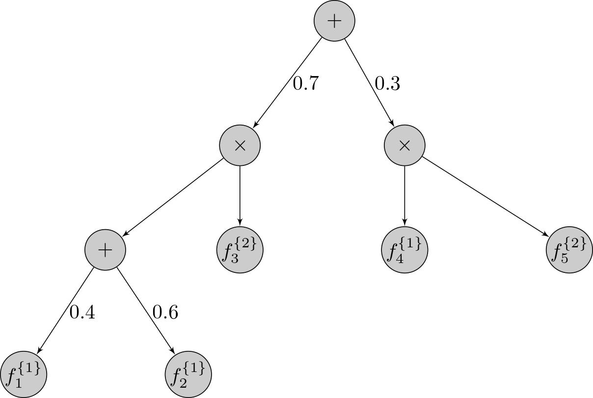
Figure 1: This figure depicts a simple SPN. Each leaf in this SPN represents a simple univariate distribution. To save space, the scope of each leaf is written in the superscript. Each + node represents a mixture distribution of its children, and its mixing weights are shown on the outgoing edges to its children. Each $\times$ node represents the product distribution of its children. The root node corresponds to the ultimate distribution that the SPN represents. The corresponding SPN signature for this SPN is the following: $\big{(}\big{(}0.7((0.4(f_{1},\{1\})+0.6(f_{2},\{1\}))\times(f_{3},\{2\}))+\\ 0.3((f_{4},\{1\})\times(f_{5},\{2\}))\big{)},~{}\{1,2\}\big{)}$.

4.2 $(\epsilon,\alpha)$Similarity and SPN Structures

In this subsection we define $(\epsilon,\alpha)$-similarity between two signatures. This property is a useful tool that will allow us to simplify our proofs. $(\epsilon,\alpha)$-similarity can also be used to formally define what it means for two signatures to have the same structure.

Roughly speaking, two signatures are $(\epsilon,\alpha)$-similar if (i) their corresponding SPNs have the same structure, and (ii) all their corresponding weights are $\alpha$-similar, and (iii) all their corresponding leaves are $\epsilon$-close in TV distance. Here is the formal definition.

Definition 10 ($(\epsilon,\alpha)$-similar).

Given parameters $\epsilon\in[0,1]$ and $\alpha\in[0,1]$, we say two signatures $s=(z,b),\hat{s}=(\hat{z},\hat{b})\in S(T_{\mathcal{F}}^{n})$ are $(\epsilon,\alpha)$-similar, $s\stackrel{{\scriptstyle\mathclap{\epsilon,\alpha}}}{{\sim}}\hat{s}$, if they satisfy one of the following three properties:

1. • $b=\hat{b}$ and

   • $z,\hat{z}\in\mathcal{F}$ and

   • $\operatorname{TV}(z,\hat{z})\leq\epsilon$

2. $\exists z_{1},\dots,z_{k},\hat{z}_{1},\dots,\hat{z}_{k}$ and $b_{1},\dots,b_{k},\hat{b}_{1},\dots,\hat{b}_{k}$ such that

   • $z=((z_{1},b_{1})\times\dots\times(z_{k},b_{k}))$ and

   • $\hat{z}=((\hat{z}_{1},b1)\times\dots\times(\hat{z}_{k},b_{k}))$ and

   • $b=\hat{b}=\bigcup\limits_{i=1}^{k}b_{i}$ and

   • $\forall i\enskip(z_{i},b_{i})\stackrel{{\scriptstyle\mathclap{\epsilon,\alpha}}}{{\sim}}(\hat{z}_{i},\hat{b}_{i})$

3. $\exists z_{1},\dots,z_{k},\hat{z}_{1},\dots,\hat{z}_{k}$ and
   $(w_{1},\dots,w_{k}),(\hat{w}_{1},\dots,\hat{w}_{k})\in\Delta_{k}$ such that

   • $z=(w_{1}(z_{1},b_{1})+\dots+w_{k}(z_{k},b_{k}))$ and

   • $\hat{z}=(\hat{w}_{1}(\hat{z}_{1},b_{1})+\dots+\hat{w}_{k}(\hat{z}_{k},b_{k}))$ and

   • $\forall i\enskip(z_{i},b)\stackrel{{\scriptstyle\mathclap{\epsilon,\alpha}}}{{\sim}}(\hat{z}_{i},\hat{b})$ and

   • $\forall i\enskip|\hat{w}_{i}-w_{i}|\leq\alpha$

We slightly abuse notation by writing $z,\hat{z}\in\mathcal{F}$ and $TV(\hat{z},z)\leq\epsilon$, since the $z$ and $\hat{z}$ are strings/symbols; yet, here we just mean the distribution in $\mathcal{F}$ that corresponds to that symbol. $(\epsilon,\alpha)$-similarity is a useful property that we will later use in our proofs.

More immediately, we need $(\epsilon,\alpha)$-similarity to formally define what it means for two signatures to have the same structure.

Definition 11 (same structure).

We say two signatures $s,\hat{s}\in S(T_{\mathcal{F}}^{n})$ have the same structure if they are $(1,1)$-similar and we denote this by $s\equiv\hat{s}$.

Note that the TV distance between two distributions is at most $1$ and the absolute difference between two weights is at most $1$. Therefore, the fact that two signatures are $(1,1)$-similar just means that their corresponding SPNs have the same structure, in the sense that the way their nodes are connected is the same, and the scope of corresponding sub trees is the same (with no actual guarantee on the “closeness” of their leaves or weights).

Note that $s\equiv\hat{s}$ is an equivalence relation, therefore we can talk about the equivalence classes of this relation. We use these equivalence classes to give the following definition.

Definition 12 (An SPN structure).

Given a signature $s\in S(T_{\mathcal{F}}^{n})$, we define an SPN structure, $[s]_{\mathcal{F}}$, as the equivalence class of $s$

$$[s]_{\mathcal{F}}\coloneqq\left\{s^{\prime}\in S(T_{\mathcal{F}}^{n}):s\equiv s^{\prime}\right\}$$

Essentially, an SPN structure is a set of signatures that represent distributions that all have the same structure. This is a useful definition as it will allow us to precisely state our results. Finally, we denote by $\textnormal{Dist}([s]_{\mathcal{F}})$ the set of all distributions that correspond to the signatures in the equivalence class $[s]_{\mathcal{F}}$. We are now ready to state our main results formally.

4.3 Main Results: Formal

The proof of these results can be found in Section 7.

Theorem 3.

Let $\mathcal{G}$ be the class of $d$-dimensional Gaussians. For every SPN structure $[s]_{\mathcal{G}}$, the class $\textnormal{Dist}\left([s]_{\mathcal{G}}\right)$ can be learned using

$$\widetilde{O}\bigg{(}\frac{ed^{2}+k}{\epsilon^{2}}\bigg{)}$$

samples, where $e$ and $k$ are the number of leaves and the number of mixing weights of (every) $f\in\textnormal{Dist}([s]_{\mathcal{F}})$ respectively.

Theorem 5.

Let $\mathcal{C}$ be the class of discrete distributions with support size $d$. For every SPN structure $[s]_{\mathcal{C}}$, the class $\textnormal{Dist}\left([s]_{\mathcal{C}}\right)$ can be learned using

$$\widetilde{O}\bigg{(}\frac{ed+k}{\epsilon^{2}}\bigg{)}$$

samples, where $e$ and $k$ are the number of leaves and the number of mixing weights of (every) $f\in\textnormal{Dist}([s]_{\mathcal{F}})$ respectively.

5 Distribution Compression Schemes

In this section we provide an overview of distribution compression schemes and their relation to PAC-learning of distributions. Distribution compression schemes were recently introduced in (Ashtiani et al., 2018a, ) as a tool to study the sample complexity of learning a class of distributions. Here, the high-level use-case of this approach is that if we show a class of distributions admits a certain notion of compression, then we can bound the sample complexity of PAC-learning with respect to that class of distributions.

Let us fix a class of distributions, $\mathcal{F}$. A distribution compression scheme for $\mathcal{F}$ consists of an encoder and a decoder. The encoder, knowing the true data distribution $f\in\mathcal{F}$, receives an i.i.d. sample $S\sim f^{m}$ of size $m$, and tries to “encode” $f$ using a small subset of $S$ and a few extra bits. On the other hand, the decoder, unaware of $f$, aims to reconstruct (an approximation of) $f$ using the given subset of samples and the bits. Roughly speaking, $\mathcal{F}$ is compressible if there exist a decoder and an encoder such that for any $f\in\mathcal{F}$, the decoder can recover (a good approximation of) $f$ based on the given information from the encoder.

More precisely, suppose that the encoder always uses “short” messages to encode any $f\in\mathcal{F}$: it uses a sequence of at most $\tau$ instances from $S$ and at most $t$ extra bits. Also, suppose that for all $f\in\mathcal{F}$, the decoder receives the encoder’s message and with high probability outputs an $\hat{f}\in\mathcal{F}$ such that $TV(f,\hat{f})\leq\epsilon$. In this case, we say that $\mathcal{F}$ admits $(\tau,t,m)$ compression, where $\tau$, $t$, and $m$ can be functions of the accuracy parameter, $\epsilon$.

The difference between this type of sample compression and the more usual notions of compression is that we not only use bits, but also use the samples themselves to encode a distribution. This extra flexibility is essential—e.g., the class of univariate Gaussian distributions (with unbounded mean) has infinite metric entropy and can be compressed only if on top of the bits we use samples to encode the distribution.

5.1 Formal Definition of Compression Schemes

In this section, we provide a formal definition of distribution compression schemes.

Definition 13 (decoder (Ashtiani et al., 2018a, )).

A decoder (Ashtiani et al., 2018a, ) for $\mathcal{F}$ is a deterministic function $\mathcal{J}:\bigcup_{n=0}^{\infty}Z^{n}\times\bigcup_{n=0}^{\infty}\{0,1\}^{n}\rightarrow\mathcal{F}$, which takes a finite sequence of elements of $Z$ and a finite sequence of bits, and outputs a member of $\mathcal{F}$.

Definition 14 (compression schemes).

Let $\tau(\epsilon),t(\epsilon),m(\epsilon):(0,1)\rightarrow\mathbb{Z}_{\geq 0}$ be functions. We say $\mathcal{F}$ admits $\left(\tau(\epsilon),t(\epsilon),m(\epsilon)\right)$ compression if there exists a decoder $\mathcal{J}$ for $\mathcal{F}$ such that for any distribution $f\in\mathcal{F}$, the following holds:

• For any $\epsilon\in(0,1)$, if a sample $S$ is drawn from $f^{m(\epsilon)}$, then with probability at least $2/3$, there exists a sequence $L$ of at most $\tau(\epsilon)$ elements of $S$, and a sequence $B$ of at most $t(\epsilon)$ bits, such that $\operatorname{TV}\left(f,\mathcal{J}(L,B)\right)\leq\epsilon$.

Briefly put, the definition states that with probability $2/3$, there is a (short) sequence $L$ of elements from $S$ and a (short) sequence $B$ of additional bits, from which $f$ can be approximately reconstructed. This probability can be increased to $1-\delta$ by generating a sample of size $m(\epsilon)\log(1/\delta)$. The following technical lemma gives an efficient compression scheme for the class of $d$-dimensional Gaussians.

Lemma 15 (Lemma 4.2 in (Ashtiani et al., 2018a, )).

For any positive integer $d$, the class $\mathcal{G}$ of $d$-dimensional Gaussians admits an

$$\big{(}~{}O(d\log(2d)),\,O(d^{2}\log(2d)\log(d/\epsilon)),\,O(d\log(2d))~{}\big{)}$$

compression scheme.

5.2 From Compression to Learning

The following theorem draws a connection between compressibility and PAC-learnability. It states that the sample complexity of PAC-learning a class of distributions can be upper bounded if the class admits a distribution compression scheme.

Theorem 16 (Compression implies learning, Theorem 3.5 in  (Ashtiani et al., 2018a, )).

Suppose $\mathcal{F}$ admits $(\tau(\epsilon),t(\epsilon),m(\epsilon))$ compression. Then $\mathcal{F}$ can be PAC-learned using

$$\widetilde{O}\left(m\Big{(}\frac{\epsilon}{6}\Big{)}+\frac{t(\epsilon/6)+\tau(\epsilon/6)}{\epsilon^{2}}\right)\textnormal{ \emph{samples.}}$$

The idea behind the proof of this theorem is simple: if a class admits a compression scheme, then the learner can try to simulate all the messages that the encoder could have possibly sent, and use the decoder on them to find the corresponding outputs. The problem then reduces to learning from a finite class of candidate distributions (see (Ashtiani et al., 2018a, ) for details).

6 Compressing SPNs

In this section we show (roughly) that if a class of distributions, $\mathcal{F}$, is compressible, then a class of SPNs with fixed structure and leaves from $\mathcal{F}$ is also compressible. We use this result as a crucial step in proving our main results. We give a full proof of the following Theorem in the supplement.

Theorem 17.

Let $\mathcal{F}$ be a class that admits $(\tau(\epsilon),t(\epsilon),m(\epsilon))$ compression. For every SPN structure $[s]_{\mathcal{F}}$, the class Dist$([s]_{\mathcal{F}})$ admits

$$\big{(}e\tau(\epsilon/3n),et(\epsilon/3n)+k\log_{2}{(3k/2\epsilon)},48m(\epsilon/3n)e\log(6e)/\epsilon\big{)}$$

compression where $k$, $e$ and $n$ are the number of weights, the number of leaves, and the dimension of the domain of the distributions in Dist$([s]_{\mathcal{F}})$, respectively.

6.1 Overview of Our Techniques

In this subsection, we give a high level overview of our technique. As was stated in Theorem 17, given an SPN structure $[s]_{\mathcal{F}}$, we want to derive a compression scheme for the class of distributions $\textnormal{Dist}([s]_{\mathcal{F}})$ as long as the class $\mathcal{F}$ is compressible. Our compression scheme utilizes an encoder and decoder for the class $\mathcal{F}$. Our encoder can encode any $f\in\textnormal{Dist}([s]_{\mathcal{F}})$ in the following way: given $m$ samples from $f$, for each leaf $f_{i}$ the encoder can likely choose a sequence of $\tau$ samples (from the $m$ samples of $f$) and $t$ bits such that a decoder for the class $\mathcal{F}$ can outputs an $\hat{f}_{i}\in\mathcal{F}$ that is an accurate approximation of $f_{i}$. Furthermore, for each sum node $j$, we discretize its mixing weights $(w_{1},\dots,w_{k_{j}})$ with high accuracy. Our discretization, $(\hat{w}_{1},\dots,\hat{w}_{k_{j}})$, can be encoded exactly using some bits.

Our decoder for the class $\textnormal{Dist}([s]_{\mathcal{F}})$ decodes the message from the encoder in the following way: Our decoder is given the discretize mixing weights for each sum node directly in the form of bits, so nothing more needs to be done for the weights. The decoder is also given $\tau$ samples and $t$ bits for each leaf $f_{i}$. We can use the decoder for the class $\mathcal{F}$ to reconstruct $\hat{f}_{i}\in\mathcal{F}$ that is an accurate approximation for $f_{i}$, with high probability. Our decoder thus outputs the reconstructed SPN $\hat{f}\in\textnormal{Dist}([s]_{\mathcal{F}})$ with leaves $\hat{f}_{i}$ and discretized mixing weights $(\hat{w}_{1},\dots,\hat{w}_{k_{j}})$ for each sum node $j$. Finally, we show that the decoders reconstruction, $\hat{f}$, is $\epsilon$-close to $f$ with high probability.

6.2 Results

In this subsection, we work towards proving a less general version of Theorem 17 that has a simpler and more intuitive proof. With this in mind, we introduce a few definitions.

Definition 18 ($\epsilon$-net).

Let $\epsilon\geq 0$. We say $N\subseteq X$ is an $\epsilon$-net for $X$ in metric $d$ if for each $x\in X$ there exists some $y\in N$ such that $d(x,y)\leq\epsilon$.

Definition 19 (path weight).

Let $e$ be the number of leaves in an SPN. For any index $i\in[e]$, the path weight, $W_{i}$, of the $i$th leaf of an SPN is the product of all the mixing weights along the unique path from the root to the $i$th leaf.

In other words, when sampling from an SPN distribution, the path weight of a leaf is the probability of getting a sample from that leaf. We say a leaf in an SPN is negligible if its path weight is less than $\epsilon/3e$, where $e$ is the number of leaves in the SPN. When we say a class of SPNs has no negligible leaves, we mean none of the distributions in the class has negligible path weights. We now proceed to prove the following lemma.

Lemma 20.

Let $\mathcal{F}$ be a class that admits $(\tau(\epsilon),t(\epsilon),m(\epsilon))$ compression. For every SPN structure $[s]_{\mathcal{F}}$, the class Dist$([s]_{\mathcal{F}})$ (with no negligible leaves), admits

$$\big{(}e\tau(\epsilon/2n),et(\epsilon/2n)+k\log_{2}{(k/\epsilon)},48m(\epsilon/2n)e\log(6e)/\epsilon\big{)}$$

compression where $k$, $e$ and $n$ are the number of weights, the number of leaves, and the dimensionality of the domain of the distributions in Dist$([s]_{\mathcal{F}})$, respectively.

To prove the above lemma, we first need to show that if two SPN signatures are $(\epsilon,\alpha)$-equivalent, then there is a direct relationship between the SPNs they represent. The proof can be found in the supplement.

Lemma 21.

Given that two signatures $s,\hat{s}\in[s]_{\mathcal{F}}$ are $(\epsilon,\alpha)$-similar, their corresponding SPNs $f,\hat{f}\in\textnormal{Dist}([s]_{\mathcal{F}})$ satisfy

$$\operatorname{TV}(\hat{f},f)\leq n\epsilon+k\alpha/2$$

where $k$ and $n$ are the number of weights in and the dimensionality of the domain of both $f$ and $\hat{f}$ respectively.

We can use the above result to prove lemma 20.

Proof of Lemma 20.

We want to show that given $48m(\epsilon/2n)e\log(6e)/\epsilon$ samples from $f$, we can construct $\hat{f}$ that is $\epsilon$-close to $f$ with probability $2/3$. For any index $i\in[e]$, the $i$-th leaf of $f$ is given by $f_{i}\in\mathcal{F}$.

Encoding: We define $m_{0}\coloneqq 48m(\epsilon/2n)e\log(6e)/\epsilon$ to be the number of samples we have from $f\in\textnormal{Dist}([s]_{\mathcal{F}})$. Since we have $m_{0}$ samples (and none of the path weights are negligible) using a standard Chernoff bound together with a union bound, there are no less than $m(\epsilon/2n)\log 6e$ samples for every leaf of $f$, with probability at least $5/6$. Given this many samples for each leaf, there exists a sequence of $\tau(\epsilon/2n)$ samples and $t(\epsilon/2n)$ bits such that a decoder for the class $\mathcal{F}$ outputs $\hat{f}_{i}\in\mathcal{F}$ that satisfies

$$\operatorname{TV}(f_{i},\hat{f}_{i})\leq\frac{\epsilon}{2n}$$ (1)

with probability no less than $1-1/6e$. Finally, using a union bound, the failure probability of our encoding is no more than $1/3$.

Let $l\in\mathbb{N}_{+}$ be the number of sum nodes. Let $j\in[l]$ be an index; for the $j$-th sum node, we can construct an $(\epsilon/k)$-net in $\ell_{\infty}$ of size $(k/\epsilon)^{k_{j}}$ for its mixing weights, where $k_{j}$ is the number of mixing weights of the $j$th sum node. There exists, in each sum node’s net, an element $(\hat{w}_{1},\dots,\hat{w}_{k_{j}})\in\Delta_{k_{j}}$ such that

$$\|(\hat{w}_{1},\dots,\hat{w}_{k_{j}})-(w_{1},\dots,w_{k_{j}})\|_{\infty}\leq\frac{\epsilon}{k}$$ (2)

For each sum node $j$, we can encode $(\hat{w}_{1},\dots,\hat{w}_{k_{j}})$ using no more than $k_{j}\log_{2}(k/\epsilon)$ bits; in total we need no more than $k\log_{2}(k/\epsilon)$ bits to encode all the weights in the SPN. Taking everything into account, we have $e\tau(\epsilon/2n)$ instances and $et(\epsilon/2n)+k\log_{2}{(k/\epsilon)}$ total bits that we use to encode the SPN $f$.

Decoding: the decoder directly receives $k\log_{2}{(k/\epsilon)}$ bits that correspond to $(\hat{w}_{1},\dots,\hat{w}_{k_{j}})$, for each sum node $j$. We also receive, for each leaf $f_{i}$, $\tau(\epsilon/2n)$ instances and $t(\epsilon/2n)$ bits such that the decoder for the class $\mathcal{F}$ outputs $\hat{f}_{i}\in\mathcal{F}$ that satisfies Equation (1). Our decoder will thus output an SPN $\hat{f}\in\textnormal{Dist}([s]_{\mathcal{F}})$ where the $i$-th leaf is $\hat{f}_{i}$ and each sum node $j$ has mixing weights $(\hat{w}_{1},\dots,\hat{w}_{k_{j}})$.

To complete the proof, we need to show that our reconstruction, $\hat{f}$ is $\epsilon$-close to $f$ with probability $2/3$. Our encoding succeeds with probability no less than $2/3$ , so we simply need to show that $\operatorname{TV}(f,\hat{f})\leq\epsilon$. Let $s$ and $\hat{s}$ represent the SPN signatures of $f$ and $\hat{f}$ respectively. By equations (1) and (2) and Definition 10, we have that $s$ and $\hat{s}$ are $(\epsilon/2n,\epsilon/k)$-similar. Using lemma 21 we have that $\operatorname{TV}(f,\hat{f})\leq\epsilon$. This completes our proof. ∎

7 Additional Proofs

In this section we prove some of the results stated in earlier sections.

7.1 Proof of Theorem 3

Proof of Theorem 3.

Let $\mathcal{G}$ be the class of $d$-dimensional Gaussians. Combining Theorem 17 and lemma 15, we have the following: for any SPN structure $[s]_{\mathcal{G}}$ the class $\textnormal{Dist}([s]_{\mathcal{G}})$ – where each distribution in $\textnormal{Dist}([s]_{\mathcal{G}})$ has $e$ leaves and has domain with dimensionality $n$ – admits a

$$\bigg{(} O\big{(}ed\log(2d)\big{)},$$

$$O\big{(}ed^{2}\log(2d)\log(3dn/\epsilon)\big{)}+k\log_{2}{(3k/\epsilon)},$$

$$O\big{(}d\log(2d)e\log(6e)/\epsilon\big{)}\bigg{)}$$

compression scheme. Using Theorem 16 shows that this class can be learned using $\widetilde{O}((ed^{2}+k)/\epsilon^{2})$ samples, which completes the proof. ∎

7.2 Proof of Theorem 5

To prove Theorem 5 we need the following lemma.

Lemma 22.

The class of discrete distributions, $\mathcal{C}$, with support size $d$ admits $(0,d\log(d/\epsilon),0)$ compression.

Proof.

The proof is quite simple. We only need to compress the $d$ parameters $(p_{1},\dots,p_{d})$ directly. We cast an $(\epsilon/d)$-net in $l_{\infty}$ of size $(\epsilon/d)^{d}$ for the $d$ parameters. There exists an element in our $(\epsilon/d)$-net, $(\hat{p}_{1},\dots,\hat{p}_{d})$, that satisfies

$$\|(\hat{p}_{1},\dots,\hat{p}_{d})-(p_{1},\dots,p_{d})\|_{\infty}\leq\frac{\epsilon}{d}$$

So for any $i\in[d]$, we have $|\hat{p}_{i}-p_{i}|\leq\epsilon/d$. We can thus encode $(\hat{p}_{1},\dots,\hat{p}_{d})$ using no more than $d\log_{2}(\epsilon/d)$ bits. The decoder receives these discretized weights (in bits) and directly outputs $\hat{f}=(\hat{p}_{1},\dots,\hat{p}_{d})$ which is $\epsilon$-close to $f$. This completes the proof. ∎

Proof of Theorem 5.

Let $\mathcal{C}$ be the class of discrete distributions with support size $d$. Combining Theorem 17 and lemma 22 we have the following: for any SPN structure $[s]_{\mathcal{C}}$ the class $\textnormal{Dist}([s]_{\mathcal{C}})$ – where each distribution in $\textnormal{Dist}([s]_{\mathcal{C}})$ has $e$ leaves and has domain with dimensionality $n$ – admits a

$$(0,ed\log_{2}(3dn/\epsilon)+k\log_{2}{(3k/\epsilon)},0)$$

compression scheme. Using Theorem 16 we have that this class can be learned using $\widetilde{O}((ed+k)/\epsilon^{2})$ samples, which completes the proof. ∎

8 Previous Work

Distribution learning is a broad topic of study and has been investigated by many scientific communities (e.g.,  (Kearns et al.,, 1994; Devroye,, 1987; Silverman,, 1986)). There are many measures of distance to choose from when one wishes to measure the similarity of two distributions. In this work we use the TV distance which has been applied to derive numerous bounds on the sample complexity of learning GMMs (Ashtiani et al., 2018a, ; Ashtiani et al., 2018b, ; Chan et al.,, 2014; Daskalakis and Kamath,, 2014; Suresh et al.,, 2014) as well as other types of distributions (see Diakonikolas, (2016); Chan et al., (2013); Diakonikolas et al., (2016) and references therein). There are many other common measures of similarity used for density estimations such as Kullback-Leibler (KL) divergence and general $L_{p}$ distances with $p>1$. Unfortunately, for the simpler problem of learning GMMs it can be shown that the sample complexity of learning with respect to KL divergence and general $L_{p}$ distances must depend on structural properties of the distribution while the same does not hold for the TV distance. For more details on this see (Ashtiani et al., 2018a, ).

Research on SPNs has primarily been focused on developing practical methods that learn appropriate structures for SPNs (Dennis and Ventura,, 2012; Gens and Pedro,, 2013; Peharz et al.,, 2013; Lee et al.,, 2013; Dennis and Ventura,, 2015; Vergari et al.,, 2015; Rahman and Gogate,, 2016; Trapp et al.,, 2016; Hsu et al.,, 2017; Dennis and Ventura,, 2017; Jaini et al., 2018a, ; Kalra et al.,, 2018; Bueff et al.,, 2018; Trapp et al.,, 2019) as well as methods that learn the parameters of SPNs (Poon and Domingos,, 2011; Gens and Domingos,, 2012; Peharz et al.,, 2014; Desana and Schnörr,, 2016; Rashwan et al.,, 2016; Zhao et al.,, 2016; Jaini et al.,, 2016; Trapp et al.,, 2018; Rashwan et al.,, 2018; Peharz et al.,, 2019). This line of research is not directly related to our work since they are interested in the development of efficient algorithms to be used in practice.

There has also been some theoretical work showing that increasing the depth of SPNs provably increases the representational power of SPNs (Martens and Medabalimi,, 2014; Delalleau and Bengio,, 2011) as well as some work showing the relationship between SPNs and other types of probabilistic models (Jaini et al., 2018b, ). Although these papers investigate theoretical properties of SPNs, they are not directly related to our work as we are interested in the question of sample complexity.

9 Discussion

Loosely put, in this work we have derived upper bounds on the sample complexity of learning the class of tree structured SPNs with Gaussian leaves and the class of tree structured SPNs with discrete leaves. Our results hold for SPNs that are in the form of rooted trees. Therefore, it would be interesting to characterize the sample complexity of learning general SPNs (in the form of rooted DAGs). Moreover, our upper bounds hold for learning in the realizable setting, thus another interesting open direction is to extend our results to the agnostic setting. Although we can provide a simple lower bound on the sample complexity of learning SPNs – based on the fact that mixture models can be viewed as a special case of SPNs – an interesting open question is whether we can determine a tighter lower bound for SPNs of arbitrary depth. We leave these directions for future work.

10 Acknowledgements

This research was supported by an NSERC Discovery Grant.

Appendix A Omitted Proofs

A.1 Proof of Lemma 21

To prove lemma 21, we need the following proposition. The following proposition is standard and can be proved, e.g., using the coupling characterization of the TV distance.

Proposition 23.

For $i\in[d]$, let $p_{i}$ and $q_{i}$ be probability distributions over the same domain $Z$. Then $\|\Pi_{i=1}^{d}p_{i}-\Pi_{i=1}^{d}q_{i}\|_{1}\leq\sum_{i=1}^{d}\|p_{i}-q_{i}\|_{1}$.

Proof of Lemma 21.

Two signatures that are $(\epsilon,\alpha)$-similar have corresponding SPNs that have the same structure. Since any SPN can be considered the composition of smaller trees (that are also SPNs), we prove this by structural induction. Note that $\operatorname{TV}(f,\hat{f})\leq n\epsilon+k\alpha/2$ implies $\|f-\hat{f}\|_{1}\leq 2n\epsilon+k\alpha$ by definition.

Base Case: Trees of height $0$ are simply leaves. By the definition of $(\epsilon,\alpha)$-similarity, two leaves are $\epsilon$-close. Thus, the inductive hypothesis is satisfied.

Inductive step:

Suppose that the root nodes of both $f$ and $\hat{f}$ have $m$ children. For $i\in[m]$, let $f_{i}$ and $\hat{f}_{i}$ be the $i$th children (that are smaller SPNs) of the root nodes of the SPNs $f$ and $\hat{f}$ respectively. Assume $\forall i\in[m]$ the inductive hypothesis holds between $f_{i}$ and $\hat{f}_{i}$. There are two possibilities for SPNs $f$ and $\hat{f}$: $1)$ They are rooted with a product node or $2)$ they are rooted with a sum node.

Case 1: The root node is a product node with $m$ children. This gives us

$$\|\hat{f}-f\|_{1} =\Big{\|}\prod_{i=1}^{m}{\hat{f}_{i}}-\prod_{i=1}^{m}{f_{i}}\Big{\|}_{1}\leq\sum_{i=1}^{m}\|\hat{f}_{i}-f_{i}\|_{1}$$

$$\leq\sum_{i=1}^{m}(2n_{i}\epsilon+k_{i}\alpha)=2n\epsilon+k\alpha$$

Where $k_{i}$ and $n_{i}$ are the number of weights in and the dimensionality of the domain of $f_{i}$ respectively. The first inequality follows from Proposition 23.

Case 2: The root node is a sum node with $m$ children. This give us

$$\|\hat{f}-f\|_{1} =\Big{\|}\sum_{i=1}^{m}(\hat{w}_{i}\hat{f_{i}}-w_{i}f_{i})\Big{\|}_{1}$$

$$\leq\Big{\|}\sum_{i=1}^{m}w_{i}(\hat{f}_{i}-f_{i})\Big{\|}_{1}+\Big{\|}\sum_{i=1}^{m}(\hat{w}_{i}-w_{i})\hat{f}_{i}\Big{\|}_{1}$$

$$\leq\sum_{i=1}^{m}w_{i}\|\hat{f}_{i}-f_{i}\|_{1}+\sum_{i=1}^{m}|\hat{w}_{i}-w_{i}|\|\hat{f}_{i}\|_{1}$$

$$\leq\sum_{i=1}^{m}w_{i}\cdot(2n\epsilon+k_{i}\alpha)+\sum_{i=1}^{m}\alpha\cdot 1$$

$$\leq 2n\epsilon\sum_{i=1}^{m}w_{i}+\bigg{(}\sum_{i=1}^{m}w_{i}\cdot\sum_{i=1}^{m}k_{i}\alpha\bigg{)}+\sum_{i=1}^{m}\alpha\cdot 1$$

$$=2n\epsilon\cdot 1+1\cdot\sum_{i=1}^{m}k_{i}\alpha+\sum_{i=1}^{m}\alpha\cdot 1$$

$$=2n\epsilon+k\alpha$$

Where the first two inequalities hold from the properties of a norm. This completes our proof. ∎

A.2 Proof of Theorem 17

The proof of Theorem 17 mirrors many aspects of the proof of Lemma 21.

Proof of Theorem 17.

We want to show that given $48m(\epsilon/3n)e\log(6e)/\epsilon$ samples from $f$, we can construct $\hat{f}$ that is $\epsilon$-close to $f$ with probability $2/3$.

Encoding: We encode the mixing weights of the sum nodes the exact same way as in the proof for Lemma 21, but we use an $(2\epsilon/3k)$-net instead of an $(\epsilon/k)$-net.

Let $i\in[e]$ be an index. Recall that a leaf $f_{i}$ is negligible if its path weight $W_{i}$ is less than $\epsilon/3e$. We can split leaves into two groups: leaves that are negligible and leaves that are non-negligible. For non-negligible leaves, using a standard Chernoff bound together with a union bound, we have $m(\epsilon/3n)\log(6e)$ samples from all non-negligible leaves with probability no less than $5/6$. Given this many samples for each non-negligible leaf, there exists a sequence of $\tau(\epsilon/3n)$ samples and $t(\epsilon/3n)$ bits such that a decoder for the class $\mathcal{F}$ outputs $\hat{f}_{i}\in\mathcal{F}$ that satisfies

$$\operatorname{TV}(f_{i},\hat{f}_{i})\leq\frac{\epsilon}{3n}$$ (3)

with probability no less than $1-1/6e$. Using a union bound, Equation 3 holds for all non-negligible leaves simultaneously with probability no less than $5/6$.

We cannot make any guarantees on the number of samples that come from negligible leaves. For each negligible leaf $f_{i}$, we pick an arbitrary sequence of $\tau(\epsilon/3n)$ samples and $t(\epsilon/3n)$ bits. The decoder for the class $\mathcal{F}$ will thus output an arbitrary $\hat{f_{i}}\in\mathcal{F}$ such that $\operatorname{TV}(f_{i},\hat{f}_{i})\leq 1$. As we will show shortly, we do not need to do any better for negligible leaves. Finally, using a union bound, the failure probability of our encoding is no more than $1/3$.

Decoding: The mixing weights for our sum nodes are decoded in the same way as as in the proof for Lemma 21. Our decoder receives a sequence of $\tau(\epsilon/3n)$ and $t(\epsilon/3n)$ bits for each leaf $f_{i}$. For non-negligible leaves, the decoder for the class $\mathcal{F}$ will output $\hat{f}_{i}\in\mathcal{F}$ that satisfies Equation (3). For non-negligible leaves, the decoder outputs also outputs an $\hat{f}_{i}\in\mathcal{F}$, but we have no guarantee of how accurately it approximates $f_{i}$. Our decoder thus outputs an SPN $\hat{f}\in\textnormal{Dist}([s]_{\mathcal{F}})$ where the $i$-th leaf is $\hat{f}_{i}$ and each sum node $j$ has mixing weights $(\hat{w}_{1},\dots,\hat{w}_{k_{j}})$.

We need to show that $\operatorname{TV}(\hat{f},f)\leq\epsilon$ with probability $2/3$. Our encoding succeeds with probability $2/3$, so we only need to show $\operatorname{TV}(\hat{f},f)\leq\epsilon$. Let $q\in\mathbb{N}$ be the number of nodes in an SPN and let $i^{\prime}\in[q]$ be an index. For any $f\in\textnormal{Dist}[s]_{\mathcal{F}}$, we can prove that any sub tree of $f$ - with at least 1 sum node in the sub tree - rooted at node $i^{\prime}$, $f_{i^{\prime}}$, and corresponding sub tree of $\hat{f}$, $\hat{f}_{i^{\prime}}$, satisfy the following:

$$\|\hat{f}_{i^{\prime}}-f_{i^{\prime}}\|_{1}\leq 2\sum_{j^{{}^{\prime}}\in N_{i^{\prime}}}W_{j^{{}^{\prime}}}^{i^{\prime}}+2\hat{n}\epsilon/3n+2\hat{k}\epsilon/3k$$

where $\hat{n}$ is the dimensionality of the domain of the sub trees, $\hat{k}$ is the number of mixing weights in the sub trees, $N_{i^{\prime}}$ is the subset of $[e]$ that represent the negligible leaves in $f_{i^{\prime}}$ and $W_{j^{{}^{\prime}}}^{i^{\prime}}$ represents the product of the mixing weights along the unique path from (negligible) leaf $j^{\prime}$ up to node $i^{\prime}$. We can prove this via induction over the height of the sub trees.

Base case: Our base case consists of two separate possibilities. All sub trees (that contain at least 1 sum node) are built on top of either: 1) A sub tree of height 1 with a single sum node and some leaves or 2) a sub tree of height 2 rooted with a sum node. The sub trees of type 2) have roots that are connected to product nodes, which are further connected to leaves.

Case 1: Let $f_{i^{\prime}}$ represent a sub tree of height 1 rooted with a sum node. Let $m$ be the number of children of $f_{i}^{\prime}$ and $\hat{f}_{i^{\prime}}$. The children of the root nodes of $f_{i^{\prime}}$ and $\hat{f_{i^{\prime}}}$ are given by $f_{k^{\prime}}$ and $\hat{f}_{k^{\prime}}$ respectively, where $k^{\prime}\in[m]$. Thus we have

$$\|\hat{f}_{i^{\prime}}-f_{i^{\prime}}\|_{1} =\Big{\|}\sum_{k^{\prime}=1}^{m}(\hat{w}_{k^{\prime}}\hat{f_{k^{\prime}}}-w_{k^{\prime}}f_{k^{\prime}})\Big{\|}_{1}\leq\Big{\|}\sum_{k^{\prime}=1}^{m}w_{k^{\prime}}(\hat{f}_{k^{\prime}}-f_{k^{\prime}})\Big{\|}_{1}+\Big{\|}\sum_{k^{\prime}=1}^{m}(\hat{w}_{k^{\prime}}-w_{k^{\prime}})\hat{f}_{k^{\prime}}\Big{\|}_{1}$$

$$\leq\sum_{k^{\prime}=1}^{m}w_{k^{\prime}}\|\hat{f}_{k^{\prime}}-f_{k^{\prime}}\|_{1}+\sum_{k^{\prime}=1}^{m}|\hat{w}_{k^{\prime}}-w_{k^{\prime}}|\|\hat{f}_{k^{\prime}}\|_{1}$$

$$=\sum_{k^{\prime}\in N_{i^{\prime}}}w_{k^{\prime}}\|\hat{f}_{k^{\prime}}-f_{k^{\prime}}\|_{1}+\sum_{k^{\prime}\not\in N_{i^{\prime}}}w_{k^{\prime}}\|\hat{f}_{k^{\prime}}-f_{k^{\prime}}\|_{1}\sum_{k^{\prime}=1}^{m}|\hat{w}_{k^{\prime}}-w_{k^{\prime}}|\|\hat{f}_{k^{\prime}}\|_{1}$$

$$\leq 2\sum_{k^{\prime}\in N_{i^{\prime}}}w_{k^{\prime}}+2\epsilon/3n+2\hat{k}\epsilon/3k\leq 2\sum_{k^{\prime}\in N_{i^{\prime}}}w_{k^{\prime}}+2\hat{n}\epsilon/3n+2\hat{k}\epsilon/3k$$

$$=2\sum_{j^{\prime}\in N_{i^{\prime}}}W_{j^{\prime}}^{i^{\prime}}+2\hat{n}\epsilon/3n+2\hat{k}\epsilon/3k$$

Case 2: Let $f_{i^{\prime}}$ represent a sub tree of height 1 rooted with a sum node. Let $m$ be the number of children of $f_{i}^{\prime}$ and $\hat{f}_{i^{\prime}}$. The children of the root nodes of $f_{i^{\prime}}$ and $\hat{f_{i^{\prime}}}$ are given by $f_{k^{\prime}}$ and $\hat{f}_{k^{\prime}}$ respectively, where $k^{\prime}\in[m]$. We define $C_{j}$ as the set of nodes that are children of node $j$. Thus we have

$$\|\hat{f}_{i^{\prime}}-f_{i^{\prime}}\|_{1} =\Big{\|}\sum_{k^{\prime}=1}^{m}(\hat{w}_{k^{\prime}}\hat{f_{k^{\prime}}}-w_{k^{\prime}}f_{k^{\prime}})\Big{\|}_{1}\leq\Big{\|}\sum_{k^{\prime}=1}^{m}w_{k^{\prime}}(\hat{f}_{k^{\prime}}-f_{k^{\prime}})\Big{\|}_{1}+\Big{\|}\sum_{k^{\prime}=1}^{m}(\hat{w}_{k^{\prime}}-w_{k^{\prime}})\hat{f}_{k^{\prime}}\Big{\|}_{1}$$

$$\leq\sum_{k^{\prime}=1}^{m}w_{k^{\prime}}\|\hat{f}_{k^{\prime}}-f_{k^{\prime}}\|_{1}+\sum_{k^{\prime}=1}^{m}|\hat{w}_{k^{\prime}}-w_{k^{\prime}}|\|\hat{f}_{k^{\prime}}\|_{1}$$

$$=\sum_{k^{\prime}=1}^{m}w_{k^{\prime}}\Big{\|}\prod_{j\in C_{k^{\prime}}}{\hat{f}_{j}}-\prod_{j\in C_{k^{\prime}}}{f_{j}}\Big{\|}_{1}+\sum_{k^{\prime}=1}|\hat{w}_{k^{\prime}}-w_{k^{\prime}}|\|\hat{f}_{k^{\prime}}\|_{1}$$

$$\leq\sum_{k^{\prime}=1}^{m}w_{k^{\prime}}\left(\sum_{j\in C_{k^{\prime}}\cap N_{k^{\prime}}}2+\sum_{j\in C_{k^{\prime}}\cap\bar{N}_{k^{\prime}}}2\epsilon/3n\right)+\sum_{k^{\prime}=1}^{m}|\hat{w}_{k^{\prime}}-w_{k^{\prime}}|\|\hat{f}_{k^{\prime}}\|_{1}$$

$$\leq 2\sum_{j^{\prime}\in N_{i^{\prime}}}w_{j^{\prime}}+2\hat{n}\epsilon/3n+2\hat{k}\epsilon/3k$$

$$=2\sum_{j^{\prime}\in N_{i^{\prime}}}W_{j^{\prime}}^{i^{\prime}}+2\hat{n}\epsilon/3n+2\hat{k}\epsilon/3k$$

Where the first two inequalities follow from the properties of a norm, and the third inequality follows from proposition 23.

Inductive Step: Let $m$ be the number of children of the root nodes of SPNs $f_{i^{\prime}}$ and $\hat{f}_{i^{\prime}}$. For SPNs $f_{i^{\prime}}$ and $\hat{f}_{i^{\prime}}$, the children of their root node are given by $f_{k^{\prime}}$ and $\hat{f}_{k^{\prime}}$ respectively, where $k^{\prime}\in[m]$ is a specific index. Assume the inductive hypothesis holds between each of the corresponding $m$ children. In the case that the root is a product node we have the following

$$\|\hat{f}_{i^{\prime}}-f_{i^{\prime}}\|_{1} =\Big{\|}\prod_{k^{\prime}=1}^{m}{\hat{f}_{k^{\prime}}}-\prod_{k^{\prime}=1}^{m}{f_{k^{\prime}}}\Big{\|}_{1}\leq\sum_{k^{\prime}=1}^{m}\|\hat{f}_{k^{\prime}}-f_{k^{\prime}}\|_{1}$$

$$\leq\sum_{k^{\prime}=1}^{m}\bigg{(}2\sum_{l^{\prime}\in N_{k^{\prime}}}W_{l^{\prime}}^{k^{\prime}}+(2\hat{k}_{k^{\prime}}\cdot\epsilon)/3k+(2\hat{n}_{k^{\prime}}\cdot\epsilon)/3n\bigg{)}$$

$$=2\sum_{j^{\prime}\in N_{i^{\prime}}}W_{j^{\prime}}^{i^{\prime}}+2\hat{k}\epsilon/3k+2\hat{n}\epsilon/3n$$

Where the first inequality holds by Proposition 23. In the case that the root node is a sum node, we have the following

$$\|\hat{f}_{i^{\prime}}-f_{i^{\prime}}\|_{1} =\Big{\|}\sum_{k^{\prime}=1}^{m}(\hat{w}_{k^{\prime}}\hat{f_{k^{\prime}}}-w_{k^{\prime}}f_{k^{\prime}})\Big{\|}_{1}\leq\Big{\|}\sum_{k^{\prime}=1}^{m}w_{k^{\prime}}(\hat{f}_{k^{\prime}}-f_{k^{\prime}})\Big{\|}_{1}+\Big{\|}\sum_{k^{\prime}=1}^{m}(\hat{w}_{k^{\prime}}-w_{k^{\prime}})\hat{f}_{k^{\prime}}\Big{\|}_{1}$$

$$\leq\sum_{k^{\prime}=1}^{m}w_{k^{\prime}}\|\hat{f}_{k^{\prime}}-f_{k^{\prime}}\|_{1}+\sum_{k^{\prime}=1}^{m}|\hat{w}_{k^{\prime}}-w_{k^{\prime}}|\|\hat{f}_{k^{\prime}}\|_{1}$$

$$\leq\sum_{k^{\prime}=1}^{m}w_{k^{\prime}}\cdot\left(2\sum_{l^{\prime}\in N_{k^{\prime}}}W_{l^{\prime}}^{k^{\prime}}+(2\hat{k}_{k^{\prime}}\cdot\epsilon)/3k+2\hat{n}\epsilon/3n\right)$$

$$\quad+\sum_{k^{\prime}=1}^{m}2\epsilon/3k\cdot 1$$

$$\leq 2\sum_{j^{\prime}\in N_{j^{\prime}}}W_{j^{\prime}}^{i^{\prime}}+2\hat{k}\epsilon/3k+2\hat{n}\epsilon/3n$$

Which proves the inductive hypothesis. Let $o$ be the root node. Clearly, for any negligible leaf $j^{\prime}$, $W_{j^{\prime}}^{o}$ is the path weight of the leaf. For the SPNs $f$ and $\hat{f}$ we have

$$\|\hat{f}-f\|_{1} \leq 2\sum_{j^{\prime}\in N_{o}}W_{j^{\prime}}^{o}+2k\epsilon/3k+2n\epsilon/3n$$

$$\leq 2\sum_{j^{\prime}\in N_{o}}\epsilon/3e+2\epsilon/3+2\epsilon/3$$

$$\leq 2\epsilon/3+2\epsilon/3+2\epsilon/3$$

$$=2\epsilon$$

Since $\operatorname{TV}(\hat{f},f)=\frac{1}{2}\|\hat{f}-f\|_{1}$, this completes the proof.

∎

References

- Adel et al., (2015) Adel, T., Balduzzi, D., and Ghodsi, A. (2015). Learning the structure of sum-product networks via an svd-based algorithm. In UAI, pages 32–41.
- (2) Ashtiani, H., Ben-David, S., Harvey, N., Liaw, C., Mehrabian, A., and Plan, Y. (2018a). Nearly tight sample complexity bounds for learning mixtures of gaussians via sample compression schemes. In Advances in Neural Information Processing Systems, pages 3412–3421.
- (3) Ashtiani, H., Ben-David, S., and Mehrabian, A. (2018b). Sample-efficient learning of mixtures. In Proceedings of the Thirty-Second AAAI Conference on Artificial Intelligence, AAAI’18, pages 2679–2686. AAAI Publications.
- Bueff et al., (2018) Bueff, A., Speichert, S., and Belle, V. (2018). Tractable querying and learning in hybrid domains via sum-product networks. arXiv preprint arXiv:1807.05464.
- Chan et al., (2013) Chan, S.-O., Diakonikolas, I., Servedio, R. A., and Sun, X. (2013). Learning mixtures of structured distributions over discrete domains. In Proceedings of the twenty-fourth annual ACM-SIAM symposium on Discrete algorithms, pages 1380–1394. Society for Industrial and Applied Mathematics.
- Chan et al., (2014) Chan, S.-O., Diakonikolas, I., Servedio, R. A., and Sun, X. (2014). Efficient density estimation via piecewise polynomial approximation. In Proceedings of the Forty-sixth Annual ACM Symposium on Theory of Computing, STOC ’14, pages 604–613, New York, NY, USA. ACM.
- Darwiche, (2003) Darwiche, A. (2003). A differential approach to inference in bayesian networks. Journal of the ACM (JACM), 50(3):280–305.
- Daskalakis and Kamath, (2014) Daskalakis, C. and Kamath, G. (2014). Faster and sample near-optimal algorithms for proper learning mixtures of gaussians. In Proceedings of The 27th Conference on Learning Theory, COLT 2014, Barcelona, Spain, June 13-15, 2014, pages 1183–1213.
- Delalleau and Bengio, (2011) Delalleau, O. and Bengio, Y. (2011). Shallow vs. deep sum-product networks. In Advances in Neural Information Processing Systems, pages 666–674.
- Dennis and Ventura, (2012) Dennis, A. and Ventura, D. (2012). Learning the architecture of sum-product networks using clustering on variables. In Advances in Neural Information Processing Systems, pages 2033–2041.
- Dennis and Ventura, (2015) Dennis, A. and Ventura, D. (2015). Greedy structure search for sum-product networks. In Twenty-Fourth International Joint Conference on Artificial Intelligence.
- Dennis and Ventura, (2017) Dennis, A. and Ventura, D. (2017). Online structure-search for sum-product networks. In 2017 16th IEEE International Conference on Machine Learning and Applications (ICMLA), pages 155–160. IEEE.
- Desana and Schnörr, (2016) Desana, M. and Schnörr, C. (2016). Learning arbitrary sum-product network leaves with expectation-maximization. arXiv preprint arXiv:1604.07243.
- Devroye, (1987) Devroye, L. (1987). A course in density estimation, volume 14 of Progress in Probability and Statistics. Birkhäuser Boston, Inc., Boston, MA.
- Devroye and Lugosi, (2001) Devroye, L. and Lugosi, G. (2001). Combinatorial methods in density estimation. Springer Series in Statistics. Springer-Verlag, New York.
- Diakonikolas, (2016) Diakonikolas, I. (2016). Learning Structured Distributions. In Peter Bühlmann, Petros Drineas, Michael Kane, and Mark van der Laan, editors, Handbook of Big Data, chapter 15. Chapman and Hall/CRC.
- Diakonikolas et al., (2016) Diakonikolas, I., Kane, D. M., and Stewart, A. (2016). Efficient robust proper learning of log-concave distributions. arXiv preprint arXiv:1606.03077.
- Gens and Domingos, (2012) Gens, R. and Domingos, P. (2012). Discriminative learning of sum-product networks. In Advances in Neural Information Processing Systems, pages 3239–3247.
- Gens and Pedro, (2013) Gens, R. and Pedro, D. (2013). Learning the structure of sum-product networks. In International conference on machine learning, pages 873–880.
- Hsu et al., (2017) Hsu, W., Kalra, A., and Poupart, P. (2017). Online structure learning for sum-product networks with gaussian leaves. arXiv preprint arXiv:1701.05265.
- (21) Jaini, P., Ghose, A., and Poupart, P. (2018a). Prometheus: Directly learning acyclic directed graph structures for sum-product networks. In International Conference on Probabilistic Graphical Models, pages 181–192.
- (22) Jaini, P., Poupart, P., and Yu, Y. (2018b). Deep homogeneous mixture models: representation, separation, and approximation. In Advances in Neural Information Processing Systems, pages 7136–7145.
- Jaini et al., (2016) Jaini, P., Rashwan, A., Zhao, H., Liu, Y., Banijamali, E., Chen, Z., and Poupart, P. (2016). Online algorithms for sum-product networks with continuous variables. In Conference on Probabilistic Graphical Models, pages 228–239.
- Kalra et al., (2018) Kalra, A., Rashwan, A., Hsu, W.-S., Poupart, P., Doshi, P., and Trimponias, G. (2018). Online structure learning for feed-forward and recurrent sum-product networks. In Advances in Neural Information Processing Systems, pages 6944–6954.
- Kearns et al., (1994) Kearns, M., Mansour, Y., Ron, D., Rubinfeld, R., Schapire, R. E., and Sellie, L. (1994). On the learnability of discrete distributions. In Proceedings of the Twenty-sixth Annual ACM Symposium on Theory of Computing, STOC ’94, pages 273–282, New York, NY, USA. ACM.
- Lee et al., (2013) Lee, S.-W., Heo, M.-O., and Zhang, B.-T. (2013). Online incremental structure learning of sum–product networks. In International Conference on Neural Information Processing, pages 220–227. Springer.
- Martens and Medabalimi, (2014) Martens, J. and Medabalimi, V. (2014). On the expressive efficiency of sum product networks. arXiv preprint arXiv:1411.7717.
- Peharz et al., (2013) Peharz, R., Geiger, B. C., and Pernkopf, F. (2013). Greedy part-wise learning of sum-product networks. In Joint European Conference on Machine Learning and Knowledge Discovery in Databases, pages 612–627. Springer.
- Peharz et al., (2014) Peharz, R., Gens, R., and Domingos, P. (2014). Learning selective sum-product networks. In LTPM workshop.
- Peharz et al., (2019) Peharz, R., Vergari, A., Stelzner, K., Molina, A., Shao, X., Trapp, M., Kersting, K., and Ghahramani, Z. (2019). Random sum-product networks: A simple but effective approach to probabilistic deep learning. image, 784(54k):6k.
- Poon and Domingos, (2011) Poon, H. and Domingos, P. (2011). Sum-product networks: A new deep architecture. In 2011 IEEE International Conference on Computer Vision Workshops (ICCV Workshops), pages 689–690. IEEE.
- Rahman and Gogate, (2016) Rahman, T. and Gogate, V. (2016). Merging strategies for sum-product networks: From trees to graphs. In UAI.
- Rashwan et al., (2018) Rashwan, A., Poupart, P., and Zhitang, C. (2018). Discriminative training of sum-product networks by extended baum-welch. In International Conference on Probabilistic Graphical Models, pages 356–367.
- Rashwan et al., (2016) Rashwan, A., Zhao, H., and Poupart, P. (2016). Online and distributed bayesian moment matching for parameter learning in sum-product networks. In Artificial Intelligence and Statistics, pages 1469–1477.
- Silverman, (1986) Silverman, B. W. (1986). Density estimation for statistics and data analysis. Monographs on Statistics and Applied Probability. Chapman & Hall, London.
- Suresh et al., (2014) Suresh, A. T., Orlitsky, A., Acharya, J., and Jafarpour, A. (2014). Near-optimal-sample estimators for spherical gaussian mixtures. In Advances in Neural Information Processing Systems, pages 1395–1403.
- Trapp et al., (2019) Trapp, M., Peharz, R., Ge, H., Pernkopf, F., and Ghahramani, Z. (2019). Bayesian learning of sum-product networks. arXiv preprint arXiv:1905.10884.
- Trapp et al., (2018) Trapp, M., Peharz, R., Rasmussen, C. E., and Pernkopf, F. (2018). Learning deep mixtures of gaussian process experts using sum-product networks. arXiv preprint arXiv:1809.04400.
- Trapp et al., (2016) Trapp, M., Peharz, R., Skowron, M., Madl, T., Pernkopf, F., and Trappl, R. (2016). Structure inference in sum-product networks using infinite sum-product trees. In NIPS Workshop on Practical Bayesian Nonparametrics.
- Vergari et al., (2015) Vergari, A., Di Mauro, N., and Esposito, F. (2015). Simplifying, regularizing and strengthening sum-product network structure learning. In Joint European Conference on Machine Learning and Knowledge Discovery in Databases, pages 343–358. Springer.
- Zhao et al., (2016) Zhao, H., Poupart, P., and Gordon, G. (2016). A unified approach for learning the parameters of sum-product networks. In Proceedings of the 30th conference on Neural Information Processing Systems (NIPS).