LyaCoLoRe: Synthetic Datasets for Current and Future Lyman-$\alpha$ Forest BAO Surveys

Abstract

The statistical power of Lyman-$\alpha$ forest Baryon Acoustic Oscillation (BAO) measurements is set to increase significantly in the coming years as new instruments such as the Dark Energy Spectroscopic Instrument deliver progressively more constraining data. Generating mock datasets for such measurements will be important for validating analysis pipelines and evaluating the effects of systematics. With such studies in mind, we present LyaCoLoRe: a package for producing synthetic Lyman-$\alpha$ forest survey datasets for BAO analyses. LyaCoLoRe transforms initial Gaussian random field skewers into skewers of transmitted flux fraction via a number of fast approximations. In this work we explain the methods of producing mock datasets used in LyaCoLoRe, and then measure correlation functions on a suite of realisations of such data. We demonstrate that we are able to recover the correct BAO signal, as well as large-scale bias parameters similar to literature values. Finally, we briefly describe methods to add further astrophysical effects to our skewers — high column density systems and metal absorbers — which act as potential complications for BAO analyses.

1 Introduction

Our understanding of the expansion history of the Universe has progressed enormously over the last quarter of a century. The discovery of accelerating expansion from the “standardisable candles” of supernovae [1, 2] brought the idea of dark energy to the fore, and it is now considered a vital component of the cosmic inventory. Indeed, efforts to improve our measurements of its properties are at the forefront of current cosmological research, and it is a primary motivation behind a number of surveys past, present and future.

Several of these surveys have focussed on using the “standard ruler” of Baryon Acoustic Oscillations (BAO) [3] in their efforts to understand the Universe’s expansion. This fixed-scale imprint on structure formation was first measured from the correlation function [4] and power spectrum [5] of galaxy samples from the Sloan Digital Sky Survey (SDSS) and 2dF Galaxy Redshift Survey respectively. A number of similar measurements have been made in subsequent years, focussing on using galaxies [e.g. 6, 7, 8, 9] and quasars (QSOs) [e.g. 10] as tracers of the matter density. These tracers cover redshift ranges $z\sim 0.1-1.0$ and $z\sim 1.2-1.7$ respectively.

An alternative tracer exists in the form of the Lyman-$\alpha$ (Ly$\alpha$) forest: a sequence of absorption features that appears in the spectra of high-$z$ QSOs as a result of Ly$\alpha$ absorption of light in the neutral hydrogen gas between QSO and observer. These spectral features thus trace the density of neutral hydrogen gas in the inter-galactic medium (IGM) along the line of sight [11]. Indeed, analytical models developed during the 1990s showed that the Ly$\alpha$ forest absorption closely traces the distribution of dark matter on scales larger than the Jeans length [e.g. 12, 13, 14]. The Ly$\alpha$ forest should, then, provide a suitable means to extend measurements of cosmic expansion via BAO to earlier in the Universe’s history. Measuring such a signal was first discussed in [15], while the 3D correlation of flux transmission was first studied in [16]. The BAO signal was first detected from measurements of the Ly$\alpha$ auto-correlation using data from data release 9 (DR9) of the Baryon Oscillation Spectroscopic Survey (BOSS) of SDSS-III [17, 18, 19], with subsequent improvements in DR11 [20] and DR12 [21], as well as DR14 of the extended Baryon Oscillation Spectroscopic Survey (eBOSS) [22]. The cross-correlation between the Ly$\alpha$ forest and QSOs was first measured in BOSS DR9 [23], with the first detection of BAO coming in DR11 [24], and improvements made in DR12 [25] and eBOSS DR14 [26].

The upcoming Dark Energy Spectroscopic Instrument (DESI) [27] will be able to advance these measurements greatly. Over the 5 years of its operation, it will measure approximately 800,000 QSO spectra with $z>2.0$, 3 times as many as in the final eBOSS dataset (approximately 270,000). Ahead of such an increase in statistical power, it is vital to be able to sufficiently test analysis pipelines to ensure that they do not introduce any biases. Equally, it is important to be able to quantify exactly how secondary astrophysical effects will impact upon BAO measurements. The best way to carry out both of these tests is through the development of mock datasets [e.g. 28, 29, 30] — synthetic realisations of a survey for which cosmological and astrophysical parameters can be easily controlled. Producing such datasets must be computationally inexpensive in order to allow for generation of a large number of realisations, but the data must also provide realistic representations of the survey itself.

In this work, we introduce a package designed to produce mock datasets for current and future Ly$\alpha$ forest BAO analyses, LyaCoLoRe. In § 2, we describe the methods used to generate such datasets, including the use of a Gaussian random field to generate the 3D correlations and the subsequent post-processing to yield realistic skewers of transmitted flux fraction. The methods to determine the optimal values of parameters used in these transformations are detailed in § 3. We then verify that the datasets are able to fulfil their purpose for BAO analyses in § 4, measuring correlation functions in the same way as recent analyses from BOSS and eBOSS. In § 5, we introduce and briefly test additional astrophysical effects that LyaCoLoRe is able to include, before summarising and concluding in § 6.

2 Making the mocks

The requirement of mocks to be computationally inexpensive but also large in volume prohibits the use of hydrodynamical or full N-body simulations in their construction. Instead, Gaussian random field methods can be used to generate a linear density field in a large box. This method does not capture non-linear evolution, generating data based solely on an initial power spectrum, but is orders of magnitude faster than state of the art simulations. From an initial Gaussian field, a number of options are available to model the physical density. Most straightforwardly, using a lognormal approximation provides a semi-analytic and physically plausible ($\rho>0$) model of the density field, but breaks down beyond weakly non-linear scales [31, 32]. Formalisms such as Lagrangian perturbation theory [see 33, for a review] can help extend to mildly non-linear scales, while COLA [34] methods subsequently use a small number of N-body code timesteps to further improve modelling of non-linearities. The choice of density approximation method depends on the scales of interest and the computational budget for the task at hand. The presence of non-linear structure is not of vital importance to BAO measurements, particularly at $z\geqslant 2$ where the Ly$\alpha$ forest is observed [19]. As such, Gaussian random field methods are well suited to the production of Ly$\alpha$ BAO mock datasets, and using a lognormal approximation for the physical density is sufficient for current analyses [28]. Studies that are more heavily dependent on accurate reproduction of small-scale effects may require alternative techniques to be used. Having generated a physical density field, tracers such as QSOs can be placed at its peaks via Poisson sampling according to an input bias and number density, and line-of-sight skewers can be drawn by interpolating within the box.

Converting density skewers to mimic the transmitted flux fraction of the Ly$\alpha$ forest then requires a significant degree of post-processing. Despite the speed of Gaussian random field methods, resolution higher than $O(1)$ Mpc/$h$ is not possible within the computational bounds of mock production due to memory limitations. As a result, the 1D power spectrum of the skewers $P_{1\mathrm{D}}(k_{\parallel})$ — the power spectrum measured only from modes lying along the line of sight of each skewer — is greatly suppressed. This subsequently affects the errors on our BAO measurements, as the 3D flux power spectrum of the Ly$\alpha$ forest has a significant contribution to its error that is proportional to the 1D power spectrum, known as aliasing noise [15]. As such, we must boost the 1D power spectrum by the addition of small-scale fluctuations in order to ensure that our BAO errors behave correctly. Further, we must convert from density to optical depth at each point of each skewer. The details of this relationship are complex, but in the context of Gaussian random field mocks we are constrained to using a simple approximation such as the fluctuating Gunn-Peterson approximation (FGPA) [35]. Methods such as those discussed in [36] offer improved physical intuition behind the structure of the Ly$\alpha$ forest, but developing techniques to apply them in the context of full-survey mock datasets is beyond the scope of this work. Finally, we must add redshift-space distortions to our skewers. These distortions occur as a result of peculiar velocities in the IGM, and we observe them as an anisotropy in measurements of power spectra and correlation functions.

In this work, we use CoLoRe [37] to generate our initial Gaussian skewers, as described in § 2.1. We then present the package LyaCoLoRe, which is able to convert CoLoRe’s output into realistic skewers of transmitted flux fraction. The methods used in this transformation are described in § 2.2. Finally, in § 2.3, we discuss the computational requirements of running both of these packages. The output skewers from LyaCoLoRe then require the addition of instrumental noise and combination with a QSO continuum before they can be considered realistic spectra. This can be carried out in the context of DESI by a package called desisim, which is not discussed in this work.

2.1 CoLoRe: Cosmological Lognormal Realisations

The LyaCoLoRe mocks originate from a program called CoLoRe, a highly parallelised code initially designed to produce large catalogues of multiple tracers with the same underlying density field [37]. In this work, we use CoLoRe’s lognormal density model for speed, though first and second order Lagrangian perturbation theory methods are also available. Making use of these functionalities would constitute a natural extension of this work, and efforts are ongoing to do so.

From this density field, CoLoRe can produce a number of observables such as cosmic shear, intensity maps, CMB lensing and integrated Sachs-Wolfe maps. Most importantly in the context of this work, it is also able to draw line-of-sight skewers from each object to a central observer, interpolating the Gaussian field at intermediate points. This final functionality makes CoLoRe well suited for Ly$\alpha$ forest mocks. The basic steps that CoLoRe takes in computing such skewers are outlined in the 5-stage process below:

1. Generate a Gaussian random field $\delta_{C}$ at $z=0$ in a Cartesian box according to an input power spectrum.

2. Compute a corresponding radial velocity in each cell using the gradient of the Newtonian gravitational potential $\phi$:

   $$v_{r}(z=0)=-\frac{2f_{0}}{3H_{0}^{2}\Omega_{M}}(\mathbf{e}_{r}\cdot\nabla)\phi(z=0),$$ (2.1)

   where $f_{0}$ is the logarithmic growth rate at $z=0$, $H_{0}$ is the Hubble constant, $\Omega_{M}$ is the matter density parameter, and $\mathbf{e}_{r}$ is the radial unit vector.

3. Calculate the redshift of each cell (taking the centre of the box as the observer) using a given input cosmology, and de-evolve the fields to that redshift using the corresponding linear growth factor.

4. Carry out a lognormal transformation of the Gaussian field, and Poisson sample it using an input number density $n(z)$ and bias $b(z)$ to obtain a set of sources (QSOs in our case).

5. Compute line-of-sight skewers from each source to the centre of the box by interpolating the initial Gaussian field and the radial velocity field.

The final output from CoLoRe is a set of QSOs and corresponding Gaussian field skewers, as well as values of cosmological variables along the skewers. The QSOs have the correct 3D clustering properties on large scales, as demonstrated briefly in Appendix A and in more detail in [37]. The skewers also have the correct 3D correlations, as demonstrated in § 4.

2.2 LyaCoLoRe

While CoLoRe is able to produce skewers with 3D, large-scale correlations matching a given input in a short timeframe, its “raw” output requires significant post-processing before it can be considered a realistic representation of the Ly$\alpha$ forest. To implement these stages of processing, we have developed a Python module under the name LyaCoLoRe. This code transforms CoLoRe’s output into realistic skewers of transmitted flux fraction. The following sections describe the key methods that LyaCoLoRe uses to do so, with each step represented visually in Figure 1.

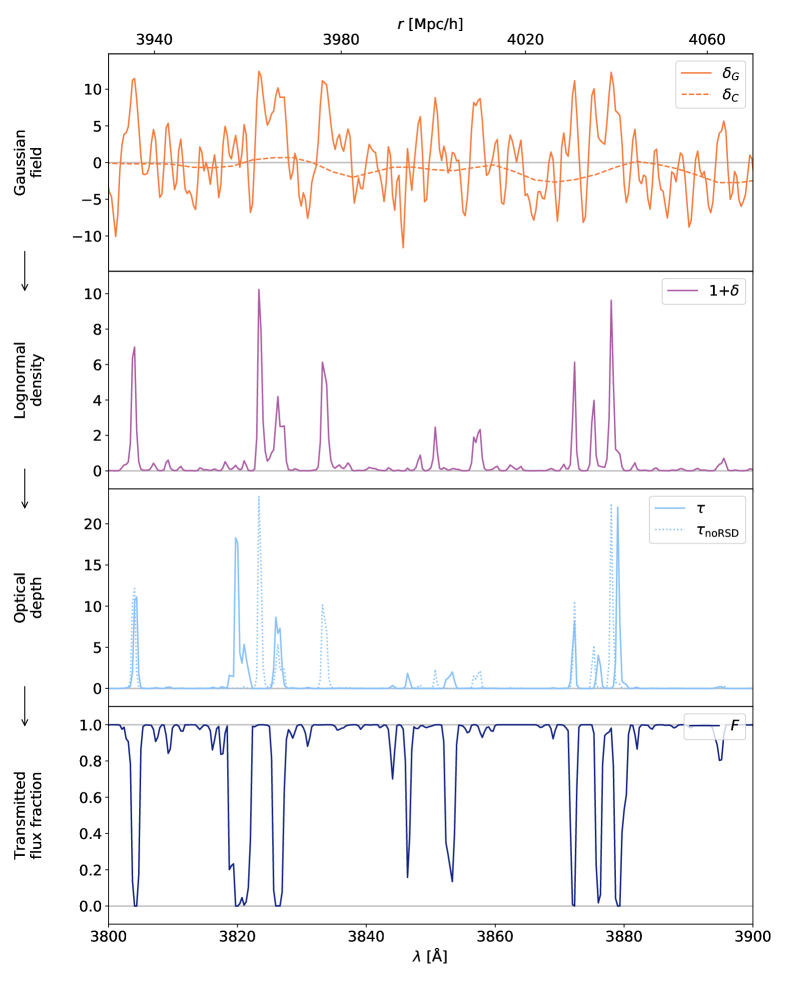
Figure 1: A sample skewer shown at the different stages of transformation from “raw” Gaussian CoLoRe output to a final LyaCoLoRe flux skewer. The top panel shows the addition of small-scale power to the skewer as described in § 2.2.1, converting $\delta_{C}$ to $\delta_{G}$. The transition to the second panel shows the lognormal transformation from § 2.2.2, and moving to the dotted line of the third panel shows the fluctuating Gunn-Peterson approximation (FGPA) transformation from the same section. The application of redshift-space distortions (RSDs), as described in § 2.2.3, shifts the dotted line to the solid line in this third panel. The final transformation from optical depth to flux, as described in § 2.2.4, maps the third to the bottom panel. Here, the Hubble flow is used to map distances (top horizontal axis) to observed wavelengths (bottom horizontal axis).

2.2.1 Adding small-scale power

In order that the memory requirements of running CoLoRe do not become overwhelmingly large, we are limited to using a grid of $4096^{3}$ cells. Requiring that this encloses the volume of a full Ly$\alpha$ survey limits us to using a low-resolution grid, with cells in CoLoRe’s raw output of $O(1)$ Mpc/$h$. In the context of the Ly$\alpha$ forest, we observe clustering on scales down to the Jeans Length, approximately 100 kpc/$h$ [38] and an order of magnitude lower than the resolution we can feasibly achieve. While BAO is a large-scale phenomenon, imposing that the synthetic data has approximately the right small-scale properties ensures that the covariance matrices in our final analyses are realistic. We address this by first interpolating CoLoRe’s Gaussian skewers — labelled as $\delta_{C}$ — to a smaller cell size, using nearest grid point (NGP) interpolation in order to avoid introducing additional smoothing.

We then generate a set of new, independent Gaussian skewers $\delta_{\epsilon}$ on the grid of smaller cells according to an input 1D power spectrum. We take the $k$-dependence of this 1D power spectrum to follow that used in [39]:

$$P_{\rm{1D}}(k)~{}\propto~{}[1~{}+~{}(k/k_{1})^{n}]^{-1},$$ (2.2)

where the normalisation is chosen to ensure unit variance. The additional skewers are then scaled by a common factor in order to control the variance in the extra power added. This factor is allowed to vary along the length of the skewers, effectively adding a redshift-dependency to the extra power. Hence, we write this factor as $\sigma_{\epsilon}(z)$. The parameters $n$ and $k_{1}$, as well as the function $\sigma_{\epsilon}(z)$ are free, and we choose them according to the process described in § 3, aiming to achieve the correct 1D power spectrum across a range of redshifts. The new skewers are then simply added to each of the existing ones to form our final Gaussian skewers $\delta_{G}$:

$$\delta_{G}(z,\textbf{x})=\delta_{C}(\textbf{x})+\sigma_{\epsilon}(z)\delta_{\epsilon}(\textbf{x}).$$ (2.3)

The top panel of Figure 1 shows a sample skewer before and after the extra small-scale power is added. As the additional skewers are independent from one another, there are no correlations between the structures added to each of the skewers. When we measure the 3D correlation function, we ignore contributions from pixel-pairs in the same skewer and so this process of adding small-scale power will not affect the 3D correlations of the Gaussian field beyond simply adding noise.

It is worth noting that we could have chosen to add extra small-scale fluctuations to the velocity field and achieved the same correct 1D power spectrum. However, allowing parameters describing extra small-scale velocities to vary freely would require the re-computation of the redshift-space distortions weights matrix (see § 2.2.3) at each step of the tuning process (see § 3). This is a considerably more time-consuming procedure than simply carrying out the inverse Fourier transform of equation (2.2). As such, we choose to only add small-scale fluctuations to the Gaussian field and assign to each of the small cells the velocity of the nearest large CoLoRe cell.

2.2.2 Transformation to optical depth

In LyaCoLoRe, the transformation from skewers of the Gaussian field to ones of optical depth is governed by two equations. The first of these is known as a lognormal transformation. This approximates the density of the baryonic matter field closely by using a lognormally-distributed variable [32], introducing a degree of non-linearity. This is normalised so that we may define a deviation $\delta$ from the mean density as:

$$1+\delta(z,\textbf{x})=\frac{\rho(z,\textbf{x})}{\overline{\rho}(z)}=\exp{}\Bigg{[}D(z)\delta_{G}(z,\textbf{x})-D^{2}(z)\frac{\sigma_{G}^{2}(z)}{2}\Bigg{]},$$ (2.4)

where $D(z)$ is the linear growth factor at redshift $z$; $\delta_{G}(z,\textbf{x})$ is the Gaussian field value from equation (2.3); $\sigma_{G}(z)$ is the standard deviation of this Gaussian field and $\rho(z,\textbf{x})$ is the lognormal density at redshift $z$ and position x. This transformation is shown by the transition from the top to the second panel in Figure 1.

The second equation allows us to transform these deviations in density into an approximation of the optical depth at each point. Assuming adiabatic expansion implies a tight relationship between temperature and density of the form $\mathrm{d}\ln T/\mathrm{d}\ln\rho=\gamma-1$ [40]. If we further assume photoionization equilibrium, the temperature of the gas approximately determines the number of neutral hydrogen atoms $n_{\mathrm{HI}}\propto\rho^{2}T^{-0.7}$ for a given baryonic matter density $\rho$ [41]. As the optical depth $\tau$ is proportional to $n_{\mathrm{HI}}$ [42], these two assumptions allow us to provide an approximation for $\tau$ given $\rho$ known as the fluctuating Gunn-Peterson approximation (FGPA) [32, 35]:

$$\tau(z,\textbf{x})=\tau_{0}(z)[1+\delta(z,\textbf{x})]^{\alpha(z)},$$ (2.5)

where $\tau_{0}(z)$ is a normalisation determined by the gas temperature and the photoionisation rate, and $\alpha(z)=2-0.7(\gamma(z)-1)$ is determined by the temperature-density relation. These parameter functions $\tau_{0}(z)$ and $\alpha(z)$ are free, and the method for choosing them is described in § 3. The transformation to optical depth is shown by the transition from the second panel to the dotted line of the third panel in Figure 1.

2.2.3 Adding redshift-space distortions

The Ly$\alpha$ forest exists as a sequence of absorption features due to the gradient in the recessional velocity of the IGM caused by the Universe’s expansion. Features are redshifted according to their distance from the observer, appearing in a spectrum at an observed wavelength $\lambda_{\mathrm{obs}}=\lambda_{\alpha}(1+z)$ for $\lambda_{\alpha}$ the Ly$\alpha$ wavelength, and $z$ the absorption redshift. However, peculiar velocities in a region of gas cause its redshift to differ from that due to expansion alone. These effects are known as redshift-space distortions (RSDs), and can be induced by a number of different effects. In particular, RSDs due to gravitationally-induced linear velocities in the IGM are calculated by CoLoRe: as mentioned in § 2.1, it produces velocity skewers quantifying this effect by calculating the gradient of the Newtonian gravitational potential.

The transition from real- to redshift-space in each skewer can be thought of as an integral over velocity space of the real-space optical depth field multiplied by a kernel $K$:

$$\tau({s})=\int\tau({x})K\Big{(}{s}-{x}-v_{r}\big{(}{x}|T({x})\big{)}\Big{)}\mathrm{d}{x},$$ (2.6)

where $x$ and $s$ are velocity coordinates along the skewer in real- and redshift-space respectively, $v_{r}$ is the radial peculiar velocity, and $T$ is the temperature. The choice of $K$ depends on the complexity of the physical effects that you wish to capture. Choosing a suitable Gaussian kernel allows the inclusion of thermal broadening effects: the apparent spreading of the gas’s optical depth contribution in redshift-space due to random thermal velocities of the gas atoms. This is implemented as an option within LyaCoLoRe, the details of which are described in Appendix B. However, we find that the width $\sigma_{v}$ of this Gaussian kernel is often smaller than the typical cell size used in LyaCoLoRe when adding small-scale fluctuations. Thus, the net effect of accounting for this physical process is small, and so for the purposes of this work we choose the most straightforward option, setting $K(x)=\delta^{D}(x)$ for $\delta^{D}$ the Dirac delta function. This shifts the optical depth along each skewer according to the peculiar velocity, and does not attempt to include any further physical effects.

In order to implement equation (2.6), we determine a matrix of weights $W_{ij}$ for each skewer to map its real-space cells $\tau^{x}_{j}$ to redshift-space cells $\tau^{s}_{i}$ via the matrix equation $\tau^{s}_{i}~{}=~{}W_{ij}\tau^{x}_{j}$. The matrix $W_{ij}$ depends on the velocities in the skewer as well as the choice of kernel $K$, and the details of its calculation can be found in Appendix B. Our implementation conserves the integrated optical depth along each line of sight (ignoring pixels which are shifted to un-observed wavelengths). The matrix $W_{ij}$ is near-diagonal and filled mostly by zeros. It can thus be stored in the form of a sparse matrix, and applied to any additional absorption transitions (see § 5.2), reducing both the computation time and memory requirements of adding RSDs to the skewers.

The addition of RSDs (without thermal broadening) to a sample optical depth skewer is shown by the transition from the dotted to the solid line in the third panel of Figure 1.

2.2.4 Final transmission skewers

In one final stage, we convert from skewers of optical depth $\tau$ to transmitted flux fraction $F$ via the equation:

$$F(s)=\exp{}\big{[}-\tau(s)\big{]},$$ (2.7)

and interpolate onto a wavelength grid of the user’s choice to obtain $F(\lambda)$, where $\lambda=\lambda_{\alpha}(1+z)$. These skewers are then written to disc.

This final transformation can be seen in the transition between the solid lines in the third and fourth panels of Figure 1. It is worth noting that, while the signal in the lognormal density deviation $1+\delta$ and optical depth $\tau$ skewers is dominated by over-dense regions, the signal in flux $F$ becomes saturated (equal to 0) at these points and does not carry a great deal of information. Rather, the intermediate density regions — where the density is high enough to cause some absorption but not so high that saturation occurs — are those from which the most information can be gleaned.

2.3 Computational requirements

In the realisations presented in this work, we specify that CoLoRe generates a $4096^{3}$ cell box as a compromise between resolution and memory usage, given the large volume that we must cover in order to realistically represent a Ly$\alpha$ forest survey. Generating approximately $7.5\mathrm{M}$ QSOs (across the whole sky) and drawing subsequent skewers produces a dataset sufficient for a DESI-like survey, allowing for a significant degree of flexibility in the final survey strategy and number densities. The computational cost of producing one such dataset is relatively low, provided suitable multi-node, multi-core computational facilities are available. Running CoLoRe using the input data and options specified in § 4.1 in parallel across 32 Haswell compute nodes (each with 32 cores and 128GB of memory) on the National Energy Research Scientific Computing Centre’s Cori machine requires approximately $18$ minutes to run, equivalent to approximately 300 CPU hours. The large number of nodes is necessary to improve the speed of the code and to satisfy its memory requirements — a total of approximately 920 GB is needed for each run of this size. If such facilities are not available, then the box size must be reduced or the resolution lowered.

The precise requirements for running LyaCoLoRe depend strongly on the exact choices of input options. As an example, converting $800\mathrm{k}$ skewers — similar to the number that will be observed by DESI — from CoLoRe’s Gaussian output to realistic transmission skewers including RSDs (though not thermal broadening effects) requires only $4$ minutes when spread across the same 32 nodes mentioned previously. If such computational facilities are not available, then running LyaCoLoRe is still possible as its memory requirements are much lower than CoLoRe.

A very small test dataset of 1000 skewers is available within the LyaCoLoRe repository. It is straightforward to run LyaCoLoRe on this data on any standard laptop to generate sample skewers or to explore the functionality of the code.

3 Parameter tuning

A number of parameters are defined in the various transformations described in § 2.2, namely $n$, $k_{1}$, $\sigma_{\epsilon}(z)$, $\tau_{0}(z)$ and $\alpha(z)$ (see equations (2.2), (2.3) and (2.5) for definitions). These are all free parameters, and we would like to be able to choose their values so that our final skewers have particular properties. Specifically, we aim to match the 1D power spectrum $P_{\mathrm{1D}}(k,z)$, mean transmitted flux fraction $\bar{F}(z)$ and large-scale bias $b_{\delta,F}(z)$ (as defined in equation (4.2)) to literature values. Ignoring RSDs and the shape of the 1D power spectrum would allow the problem to be treated analytically, but unfortunately such simplifications are unrealistic. As such, it is not obvious how to choose our parameters correctly, and a more complex process is necessary.

We aim to solve this problem via a minimisation process. We first define a function that we will aim to minimise, and which takes the following steps:

1. Generate sample skewers in $F$ corresponding to a given set of parameter values using the methods described in § 2.2.

2. Measure the 1D power spectrum, mean flux and large-scale bias of these skewers at a selection of redshift values.

3. Evaluate the deviation of each measurement at each redshift from literature results.

4. Quantify this deviation with a single number.

In step 2, we measure $P_{\mathrm{1D}}$ and $\bar{F}$ straightforwardly, excluding cells that sit at a rest frame wavelength above $1200\ \mbox{\AA}$. We measure $b_{\delta,F}$ by calculating the response of $\bar{F}$ to a small deviation in the average density field: $b_{\delta,F}=(1/\bar{F})\ \mathrm{d}\bar{F}/\mathrm{d}\delta$ [43]. The literature values referred to in step 3 are the fitting function from the BOSS DR9 $P_{\mathrm{1D}}$ measurement from [44], the fitting function of the mean flux measurement from [45] and the bias value and redshift evolution determined by the BOSS DR12 combined Ly$\alpha$ auto- and cross-correlation analysis in [25]. Using these literature results as targets, we compute a weighted error for each measurement at each redshift value. When computing the error on the $P_{\mathrm{1D}}$, we prioritise the low-$k$ modes by using a $k$-dependent error weighting. For $k<0.02\ \mathrm{s\ km}^{-1}$, this is proportional to $1/(1+(k/k_{0})^{2})$ where $k_{0}=0.01\ \mathrm{s\ km}^{-1}$. This ensures the modes most relevant for a BAO analysis — those with $k\lessapprox 0.005\ \mathrm{s\ km}^{-1}$ [15, 46] — are prioritised over less important, high-$k$ modes. Beyond $k=0.02\ \mathrm{s\ km}^{-1}$, we ignore any errors as our finite cell size makes it unreasonable to expect realistic power at these scales, and these modes were not measured by BOSS. We sum the errors in quadrature over all $k$-modes using this weighting to produce an overall error on $P_{\mathrm{1D}}$. In step 4, the errors on each measurement at each redshift value are summed in quadrature, and a single number produced. This number quantifies how well a given parameter set is able to produce realistic data, as measured by our specified properties. A standard minimisation routine can then be used to minimise it over the space of input parameters. We use Minuit [47], as implemented by the python module iminuit to do so.

We introduce a number of simplifications to improve the speed of the minimisation. We assume that $\log\tau_{0}$ and $\log\sigma_{\epsilon}$ follow the functional form:

$$\log(X)=A_{0}+A_{1}\log[(1+z)/(1+z_{0})],$$ (3.1)

where $z_{0}=3.0$ and the $A_{i}$ are scalar parameters. In the case of $X=\tau_{0}$, we fix $A_{1}=4.5$ [48]. Further, we assume that $\alpha(z)$ takes a constant value of 1.65 across redshifts [49] (equivalent to a value of $\gamma=(2-\alpha)/0.7+1$ of 1.5, in reasonable agreement with the literature [e.g. 50, 51]). With these simplifications, we end up with a 5-parameter minimisation problem: 1 parameter describing the normalisation of $\tau_{0}(z)$; 2 describing the normalisation and $z$-dependence of $\sigma_{\epsilon}(z)$; and 2 describing the shape of the 1D power of the small scale fluctuations ($n$ and $k_{1}$). At each call of the routine, we produce sample skewers at a point in parameter space, and compute their 1D power spectra, mean flux and bias parameter values in 7 redshift bins of width $\Delta z=0.2$ centred at points evenly spaced between $z=2.0$ and 3.2. We run this procedure using $\sim 55,000$ skewers to obtain an initial estimate, and increase this to $\sim 220,000$ skewers in order to fine tune the optimisation.

We also introduce a parameter $a_{v}$ by which we multiply the velocities in our skewers in order to match the amount of anisotropy in the clustering of the Ly$\alpha$ forest to literature values. This is not because the velocities from CoLoRe are incorrect — when using CoLoRe’s unmodified velocities, we obtain the correct level of anisotropy in the QSO auto-correlation (see Appendix A) — but is a result of the approximations in our recipe to estimate $F$. These approximations define the relationship between CoLoRe’s initial Gaussian field and our final flux skewers, and thus their inherent assumptions will affect the large-scale flux biases. While the density bias $b_{\delta}$ is matched to literature values in our tuning process, this is not the case for the RSD parameter $\beta$ (defined in § 4.3). As such, the somewhat crude nature of our approximations results in an unrealistic value of $\beta$, and we must introduce our parameter $a_{v}$ in order to correct for this shortcoming. Improving on our approximations by using more detailed modelling [e.g. 36] might allow us to avoid introducing $a_{v}$, but that is beyond the scope of this work. We fix $a_{v}=1.3$ when tuning; it is computationally costly to leave it free as a change in $a_{v}$ requires re-computation of the RSD weights matrix $W_{ij}$ (see § 2.2.3). The value is chosen on an ad hoc basis to match approximately the RSD parameter $\beta$ measured from BOSS DR12 data [25].

The final values of the transformation parameters are $\log[\tau_{0}(z)]=1.48+4.5\log x$, $\alpha(z)=1.65$, $\log[\sigma_{\epsilon}(z)]=6.02+0.276\log x$, $n=0.732$, $k_{1}=0.0341$ and $a_{v}=1.3$, where $x=[(1+z)/(1+z_{0})]$ and numerical values are rounded to three significant figures where appropriate. These are the default values used by LyaCoLoRe. The tuning process is effective, matching literature values of $P_{\mathrm{1D}}$, $\bar{F}$ and $b_{\delta,F}$ to within 10% at almost all relevant $k$-modes and $z$ values. As an example, the $P_{\mathrm{1D}}$ measured across $\sim 7.5$M skewers is shown in Figure 2. We only plot 4 redshift bins and a limited number of $k$-modes here for clearer visualisation.

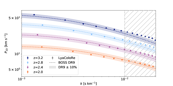
Figure 2: The 1D power spectrum as measured from one realisation of LyaCoLoRe mocks. The tuning process aims to match the measured $P_{\mathrm{1D}}$ to that from BOSS DR9 data [44] for $k$-modes that affect BAO analysis, as described in detail in § 3. Modes to the left of the dot-dash line at $k=0.01~{}\mathrm{s\ km}^{-1}$ are the most important in this respect [15, 46], and these all lie within 10% of our target $P_{\mathrm{1D}}$, as indicated by the shaded areas. Modes to the right of the dot-dash line are not important in the context of BAO, and are not prioritised in our tuning procedure.

4 Verifying the mocks

The primary motivation for creating the LyaCoLoRe mocks is to provide realistic sets of test skewers for BAO analyses from Ly$\alpha$ forest surveys. Evidently then, it is important to verify that the fundamental physical quantities studied by such analyses are correctly reproduced in the mock datasets. We thus seek to test that the BAO signal is present and unbiased in our mock datasets. § 4.1 describes the inputs we use in generating a collection of mock datasets; § 4.2 explains how we measure the correlation functions from each realisation, taking the skewers in $F$ directly from LyaCoLoRe’s output; and finally § 4.3 shows how we fit to a model. We do not visually compare the correlation functions measured from mocks to those from data, since our mock measurements are not affected by distortions from continuum fitting. Instead we compare fitted parameter values in order to assess the performance of our mock datasets.

4.1 Generating realisations

The input power spectrum that we use in step 1 of § 2.1 is generated by the Boltzmann solver CAMB [52] using the Planck Collaboration’s 2015 parameters for a flat, $\Lambda$CDM cosmology [see column 1 of Table 3 in 53]. We generate the field in a box of $4096^{3}$ cells, stipulating that this covers a redshift range $0.0\leqslant z\leqslant 3.79$: a volume large enough to contain a DESI-like survey. This results in a grid of total size $\sim(9.8\ \mathrm{Gpc/}h)^{3}$, with each cell $\sim(2.4\ \mathrm{Mpc/}h)^{3}$ in dimensions. The QSO number density function is based on estimates from SDSS-III data in Stripe 82 [54]. This is considered to represent an optimistic estimate of the photometric capability of targeting for DESI, and results in $\sim 3.7$M QSOs above $z=1.8$ across the whole sky. We use as an input QSO bias the fitting function defined in equation 19 of [55], which is based on clustering measurements from the BOSS DR12 QSO sample [56]. When running LyaCoLoRe, we use a cell size of 0.25 Mpc/$h$, and tune the parameters of our transformations according to the methods described in § 3.

For the purposes of this work we generate 10 such realisations, each with unique random seeds, and stack our results in order to test LyaCoLoRe as stringently as possible. This is approximately equivalent to 30 times the final number of Ly$\alpha$ QSOs with $z\geq 2.1$ that will be observed by DESI. It is worth noting that the signal to noise ratio will be significantly greater than 30 times that of DESI, as our skewers of $F(\lambda)$ do not include any instrumental noise, nor do they require any continuum fitting (as mentioned in § 2).

4.2 Measuring correlation functions

We test the BAO signal in our mock realisations in the standard way, by measuring correlation functions using the contrast in flux transmission:

$$\delta_{F}(\lambda)=\frac{F(\lambda)}{\bar{F}(\lambda)}-1,$$ (4.1)

where $\bar{F}(\lambda)$ is the mean value of $F(\lambda)$ in each pixel over all skewers for which that cell corresponds to rest-frame wavelength $\lambda_{r}\in[1040,1200]\ \mbox{\AA}$. The skewers of $F(\lambda)$ are taken straight from the processes described in § 2, with no further steps such as addition of continua or instrumental noise. This allows us to test the methods of § 2 to as high a degree of precision as possible, but consequently our covariance matrices may not necessarily be representative of true measurements.

We would like to measure the 3D Ly$\alpha$ auto-correlation and the 3D Ly$\alpha$-QSO cross-correlation, the standard measurements made by recent Ly$\alpha$ BAO analyses from BOSS and eBOSS. Both are estimated using the Package for IGM Cosmological-Correlations Analyses (picca). We measure these correlations separately in 3,072 HEALPix [57] pixels on the sky for each of the 10 realisations, and treat the resultant measurements as a set of 30,720 independent subsamples. In order to compute the correlation functions more quickly, we rebin pixels in our final transmission skewers into larger pixels of width $3\times 10^{-4}$ log(Å) in log-wavelength. This enables us to use a larger number of skewers and thus reduce our errors, without compromising the large-scale properties of the correlations or incurring large computational costs.

Our computation of the 3D Ly$\alpha$ auto-correlation follows that of recent Ly$\alpha$ forest BAO analyses [21, 22]. We first define a grid of bins in parallel and perpendicular separation between pairs of pixels — $r_{\parallel}$ and $r_{\perp}$ respectively — where each bin is 4 Mpc/$h$ $\times$ 4 Mpc/$h$ in size, and the maximum separation is 200 Mpc/$h$ in each direction. Pixel pairs are assigned to one of these bins by using a fiducial cosmology to convert from wavelength and angular separations to comoving distances parallel and perpendicular to the line-of-sight. The correlation is then computed as a weighted sum of products of pixel pairs of $\delta_{F}$ within each bin. We restrict ourselves to include only contributions from the Ly$\alpha$ absorption in the Ly$\alpha$ region, ignoring delta pixels outside the rest-frame wavelength range [1040,1200] Å. The covariance matrix is estimated straightforwardly by calculating the scatter between our set of 30,720 subsamples.

The 3D Ly$\alpha$-QSO cross-correlation is also computed in line with recent analyses of BOSS and eBOSS data [25, 26], as a weighted sum of pixels of $\delta_{F}$ within bins of parallel and perpendicular separation. We use the same bin size as in the auto-correlation, but are able to extend our minimum value of $r_{\parallel}$ to $-200$ Mpc/$h$ as the pixel-pixel pair symmetry of the auto-correlation is not present in the pixel-QSO pairs of the cross-correlation. As for the Ly$\alpha$ auto-correlation, we restrict the rest-frame wavelength range of our $\delta_{F}$ pixels to [1040,1200] Å, and we estimate our covariance matrix from the scatter between our 30,720 subsamples.

4.3 Fitting the correlation functions

Having measured the 3D Ly$\alpha$ auto- and Ly$\alpha$-QSO cross- correlations, we fit a model to our measurements to obtain the location of the BAO peak and check that no significant shift has been introduced. We also seek to measure the bias parameters of our tracers: Ly$\alpha$ flux $F$ and QSOs. These are defined by the relationship between the power spectra of the tracers, $P_{F}(\mathbf{k})$ and $P_{\mathrm{QSO}}(\mathbf{k})$, and the power spectrum of dark matter $P(\mathbf{k})$ [58]:

$$P_{F}(\mathbf{k})=[b_{\delta,F}+b_{\eta,F}f\mu^{2}]^{2}P(\mathbf{k}),$$ (4.2)

$$P_{\mathrm{QSO}}(\mathbf{k})=[b_{\delta,\mathrm{QSO}}+f\mu^{2}]^{2}P(\mathbf{k}).$$ (4.3)

Here, the large-scale biases of flux and QSOs are $b_{\delta,F}$ and $b_{\delta,\mathrm{QSO}}$. The parameter $b_{\eta,F}$ is the velocity gradient bias of flux, which serves to quantify the effect of RSDs. This is often expressed alternatively using $\beta=fb_{\eta,F}/b_{\delta,F}$. The value of $b_{\eta,QSO}$ is 1 by default as QSOs are conserved under RSDs (unlike $F$) and so it is held fixed [58]. The Ly$\alpha$-QSO cross- power spectrum follows naturally from (4.2) and (4.3) as:

$$P_{F\times\mathrm{QSO}}(\mathbf{k})=[b_{\delta,F}+b_{\eta,F}f\mu^{2}][b_{\delta,\mathrm{QSO}}+f\mu^{2}]P(\mathbf{k}).$$ (4.4)

We fit a model of the correlation functions to each of the measurements individually, and then to both correlations jointly. We use the same models as recent eBOSS analyses [22, 26] but ignore terms relating to systematics not present in our realisations, such as metal absorbers and high column density systems (HCDs). As we do not add continua to our skewers, we need not worry about the distortion of the correlations by the removal of long wavelength modes in the continuum fitting process, as occurs in real analyses. Thus, we do not need to consider distortion matrices, the standard method for taking these effects into account [introduced for the auto- and cross- correlations respectively in 21, 25]. The relevant terms are described using Kaiser models [58], as described in section 4.1 of [22] for the Ly$\alpha$ auto-correlation, and section 5.1 of [26] for the Ly$\alpha$-QSO cross-correlation. We use the same cosmology as used to generate the input power spectrum of CoLoRe to produce the smooth and peak components of the fiducial model power spectrum.

The fit is carried out leaving free the parameters describing the position of the BAO peak in the perpendicular and parallel directions:

$$\alpha_{\parallel}=\frac{D_{H}(z)/r_{d}}{[D_{H}(z)/r_{d}]_{\rm{fid}}},\ \ \alpha_{\perp}=\frac{D_{A}(z)/r_{d}}{[D_{A}(z)/r_{d}]_{\rm{fid}}},$$ (4.5)

where $D_{H}(z)=c/H(z)$, as well as parameters describing the bias and RSDs of the Ly$\alpha$-forest, $b_{\eta,F}$ and $\beta_{F}=fb_{\eta,F}/b_{\delta,F}$. We also leave free 2 parameters that describe the smoothing of the model power spectrum in the parallel and perpendicular directions, which help to account for the effects of the low-resolution of our CoLoRe grid. When fitting the Ly$\alpha$-QSO cross-correlation individually, we fix the value of the QSO bias $b_{\delta,\mathrm{QSO}}$ to the input value in order to avoid degeneracies, though when we fit jointly with the Ly$\alpha$ auto-correlation we are able to leave it free.

Having defined our models, the fits are then carried out using picca. We fit only on separations $40<r$ [Mpc/$h]<160$ as the lognormal density approximation used in both CoLoRe and LyaCoLoRe begins to break down on scales smaller than this, and we are not able to fit the shape of the correlation function well at these separations. Further, the QSOs cannot be expected to be correctly clustered on the smallest scales due to the low-resolution of the CoLoRe box. To determine an effective redshift of our measurements, we consider pixel-pixel/pixel-QSO pairs which fall in bins $A$ which satisfy $80<r_{A}\ [\mathrm{Mpc}/h]\ <120$, i.e. the bins that cover the BAO peak. The value of $z_{\mathrm{eff}}$ is then given by a weighted average of the redshifts of pairs in these bins.

The measured Ly$\alpha$ auto- and Ly$\alpha$-QSO cross-correlations are shown in the left and right panels of Figure 3 respectively, along with the model from the combined fit. We plot the correlations as $\xi(r)$ in bins of $|\mu|=|r_{\parallel}|/r$, where $|\mu|$ close to 0 indicates correlations close to perpendicular to the line of sight, and $|\mu|$ close to 1 indicates correlations close to parallel to the line of sight. The model appears to be a good fit to the measurement on the scales that we fit over, and the BAO peak is correctly placed. The two measurements deviate slightly from the model either side of the BAO bump in the highest $|\mu|$ bin, but this deviation is very small and is noticeable due to the extremely small error bars on our measurements.

The parameters from the individual and combined fits are shown in Table 1. The $\alpha$ parameters for each fit are all consistent with 1 to within $1\sigma$. Any deviation in the $\alpha$ parameters from 1 is certainly less than 0.2%, and so can be considered insignificant in the context of a DESI-like survey. Thus, the mock production pipeline up to this stage can be said to introduce no clear systematic bias within the capabilities of a current or near-future instrument.

In order to compare the values of biases and $\beta$s to BOSS DR12 values [table 4 of 25], we first use the published functional forms of each parameter’s redshift evolution to match the effective redshift of the BOSS DR12 measurements to that of our measurements. Having done so, we find that the two sets of values are very similar, with our measurements all lying within the 1$\sigma$ errors on the BOSS DR12 values. In particular, the values of $b_{\delta,F}$ in each of our fits are almost identical to the BOSS DR12 value, demonstrating the effectiveness of our tuning of this parameter (see § 3). We do not compare the value of $\beta_{\mathrm{QSO}}$ to BOSS DR12 measurements as our input QSO bias takes a different value at this redshift. However, the value of $b_{\delta,\mathrm{QSO}}$ deduced from the joint fit is consistent with the input value (as shown at the bottom of the column showing the Ly$\alpha$-QSO only fit). As such, we can consider the mocks to fulfil the basic criteria required of them, and thus they appear sufficient for a DESI-like survey. We do not assess the $\chi^{2}$ of the fits as we do not expect our covariance matrices to be representative of those one would expect from a real survey given the lack of noise in our skewers.

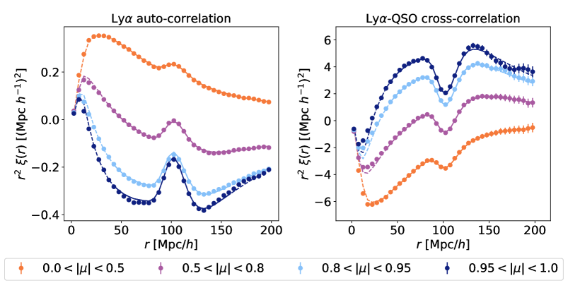
Figure 3: The correlation functions measured from 10 realisations of LyaCoLoRe datasets combined, and the best fit lines with parameters as described in the third column of Table 1. The left panel shows the Ly$\alpha$ auto-correlation, while the right panel shows the Ly$\alpha$-QSO cross-correlation. Each plot panel shows the same 4 bins in $|\mu|=|r_{\parallel}|/r$. Note that the correlations presented here do not have any distortion from continuum-fitting and so should not be visually compared with the equivalent plots from recent BOSS/eBOSS data.

	$-$LyaCoLoRe$0$			$-$BOSS DR12
Parameter	$-$Ly$\alpha$$0$	$-$Ly$\alpha$-QSO$0$	$-$Ly$\alpha$ $+$$0$	$-$Ly$\alpha$ $+$
name			$-$Ly$\alpha$-QSO$0$	$-$Ly$\alpha$-QSO
$\alpha_{\parallel}$	$-$$1.000\pm 0.002$$0$	$-$$1.001\pm 0.002$$0$	$-$$1.000\pm 0.001$$0$
$\alpha_{\perp}$	$-$$0.998\pm 0.002$$0$	$-$$1.000\pm 0.002$$0$	$-$$0.999\pm 0.001$$0$
$b_{\eta,F}$	$-0.204\pm 0.0004$	$-0.201\pm 0.0009$	$-0.203\pm 0.0004$	$-0.206\pm 0.012$
$\beta_{F}$	$-$$1.627\pm 0.008$$0$	$-$$1.624\pm 0.012$$0$	$-$$1.624\pm 0.007$$0$	$-$$1.650\pm 0.081$
$\beta_{\mathrm{QSO}}$		$0.261$	$-$$0.261\pm 0.0007$
$b_{\delta,F}$	$-0.121\pm 0.0006$	$-0.120\pm 0.0009$	$-0.121\pm 0.0005$	$-0.121\pm 0.004$
$b_{\mathrm{QSO}}$		$3.701$	$-$$3.700\pm 0.009$$0$

Table 1: Parameters from model fits of the Ly$\alpha$ auto-correlation and Ly$\alpha$-QSO cross-correlation functions measured from 10 realisations of LyaCoLoRe mocks combined. The relevant results from the BOSS DR12 combined fit [25] — those to which our values of $b_{\delta,F}$ and $b_{\eta,F}$ are tuned — are presented in the rightmost column at the same effective redshift as our measurements. The parameters in the first segment of the table are those used in the minimisation process which determines the best fit to our correlations, while those in the second segment are calculated subsequently.

5 Adding secondary astrophysical effects

A key purpose of creating mock datasets is to quantify the impact of secondary astrophysical effects on our measurements so that we may assess any biases that they could induce in our cosmological inference. When generating realisations of the synthetic data, we may choose to add or not to add different effects to each realisation, or to vary the strength of a given effect across a range of values. The resultant impact on BAO measurements can then be quantified. In Ly$\alpha$ forest analyses, two of the most pertinent effects are the presence of high column density systems (HCDs) and additional absorption transitions. LyaCoLoRe is able to compute both of these effects, and the methods it uses to do so are described in § 5.1 and § 5.2 respectively (alternative implementations of these effects are also possible). Once computed, LyaCoLoRe stores skewers of metal absorption and a table of HCDs in its output. These can then be added to the Ly$\alpha$ skewers during subsequent stages of the pipeline by packages such as desisim.

We do not present here a full study of the effects of HCDs and additional transitions on a BAO analysis. Rather, we simply illustrate in § 5.3 that their implementations within LyaCoLoRe are broadly correct and achieve the correct levels of clustering. We leave the study of these effects as systematics in a BAO analysis for future work.

5.1 Adding HCDs

HCDs occur in particularly dense regions of gas, and contain a number of subclasses determined by HI column density. Typically, we define regions with column density $N_{\mathrm{HI}}>2\times 10^{20}\ \mathrm{cm}^{-2}$ as Damped Ly$\alpha$ absorbers (DLAs), and regions with column density $10^{17.2}<N_{\mathrm{HI}}<2\times 10^{20}\ \mathrm{cm}^{-2}$ as Lyman Limit Systems (LLSs) [59]. In detailed Ly$\alpha$ forest analyses, it is important to be able to identify HCDs as their high densities broaden their absorption profiles, impacting on inferred values of $F$ over a significant wavelength range [60, 61]. Further, HCDs are of scientific interest in and of themselves [e.g. 62, 63, 64, 65, 66]. As such, being able to add HCDs to our mocks is important in maximising their realism.

We first determine potential HCD locations by computing a threshold value of the Gaussian field, set by an input bias $b_{\mathrm{HCD}}(z)$. In our realisations, we choose $b_{\mathrm{HCD}}(z)=2.0$ to be constant with redshift, and in line with [66]. This picks out peaks in the field that are sufficiently dense to host an HCD. We then Poisson sample the potential locations according to an input number density $n_{\mathrm{HCD}}(z)$. This number density is imported from the default model of the IGM physics package pyigm [67], which is fitted to a selection of literature results [summarised in Table 1 of 68]. The sampling is carried out before adding small-scale power (§ 2.2.1), as we would like the HCDs to correlate with the 3D fluctuations rather than the 1D extra power. A column density is then allocated to each HCD using a given redshift distribution — again from the default model of pyigm — and a radial velocity is determined using CoLoRe’s output. The resulting catalogue of HCDs can then be interpreted by a package such as desisim, which is able to calculate the absorption profile of the HCD using a Voigt template, and insert it into the final spectrum.

5.2 Including additional absorption transitions

As with HCDs, absorption from additional transitions are an important level of detail to add to our mocks and are of significant scientific interest [e.g. 69, 70, 55, 71]. Additional transitions have a rest-frame absorption wavelength different to that of Ly$\alpha$, and so absorption from gas at the same redshift appears at different observed wavelengths in spectra. Conversely, absorption from two different transitions can appear at the same observed wavelength even though the regions of gas hosting the absorbers are far apart physically. As a result, the presence of such absorption transitions acts to contaminate our measurements of Ly$\alpha$ flux, and thus our correlation functions and resultant BAO measurements. Such transitions include Lyman-$\beta$ (Ly$\beta$), as well as from silicon, oxygen and carbon gas, for example.

Similar to the method to add HCDs described in § 5.1, it would also be reasonable to place additional absorption transitions using a Poisson-sampled “density-peak” approach, as metals are typically produced in high density regions of the universe. However, we choose to follow the methods of previous works [16, 30], assuming that the optical depth of each additional transition is proportional to that of the Ly$\alpha$ absorber. In the context of these mocks, the most important feature of these additional transitions that we seek to replicate is the strength of their 3D clustering, as it is this that will quantify any impact upon BAO measurements. In order to do so, we simply require an absorption strength (relative to Ly$\alpha$) and a rest frame wavelength for each additional transition that we wish to include. Having calculated the skewers of optical depth in real space, we scale them differently for each absorption transition according to the transition’s relative strength. For an additional transition $X$, we obtain $\tau_{X}=A_{X}\tau_{\alpha}$, where $A_{X}$ is the relative strength and $\tau_{\alpha}$ is the Ly$\alpha$ optical depth as defined in equation (2.5). We then apply RSDs (using the same weights matrix $W_{ij}$ as for Ly$\alpha$), and convert to $F_{X}(\lambda)$ separately for each $X$ according to its rest frame wavelength. For each line of sight, the separate $F_{X}(\lambda)$ skewers are then interpolated onto a common wavelength grid and are combined multiplicatively.

This method ensures that RSDs are correctly applied to each additional absorption transition, and we may tune the absorption strength in order to achieve the correct large-scale bias — and thus the correct 3D clustering — for each transition. A small selection of additional transitions and their relative strengths are shown in Table 2. These are the transitions most important to a Ly$\alpha$ BAO analysis, though further transitions can be added straightforwardly if needed. These strengths have been tuned to approximately match bias values presented in the literature [21, 25, 22].

Name	Rest frame	Relative
	wavelength [Å]	absorption strength
Ly$\alpha$	1215.67	$1.0$
Ly$\beta$	1025.72	$0.1901$
SiII (1260)	1260.42	$0$$0$$3.542\times 10^{-4}$
SiIII (1207)	1206.50	$0$$1.8919\times 10^{-3}$
SiII (1193)	1193.29	$0$$9.0776\times 10^{-4}$
SiII (1190)	1190.42	$1.28478\times 10^{-4}$

Table 2: Details of a small selection of additional absorption transition that can be used in LyaCoLoRe. The absorption strength for each absorber $X$ has been tuned to match approximately the bias value $b_{\delta,X}$ found in literature [21, 25, 22]. It is possible to add more absorbers straightforwardly, but the absorption strengths have not been calibrated beyond those listed above. These absorbers are those included in the skewers from which the correlation function in Figure 4 is measured.

5.3 Testing astrophysical effects

We assess the methods of § 5.1 and § 5.2 by first computing the 3D Ly$\alpha$-HCD cross-correlation. The methods used to do so are largely the same as used to compute the 3D Ly$\alpha$-QSO cross-correlation, as described in § 4.2. One significant difference is that we restrict the HCDs in our calculation of the Ly$\alpha$-HCD cross-correlation to lie in the rest frame wavelength range $[1040,1100]$ Å, far from the background QSO. This restriction is necessary to prevent the correlation between Ly$\alpha$ flux and QSOs from significantly affecting our measurements close to the line of sight, as is discussed further in Appendix C. An effect can still be seen in the two $\mu$-bins closest to the line of sight at large values of $r$, though this is mostly beyond the fitted range and so we are still able to measure the degree of clustering in the HCDs well. Future studies may prefer to model this effect in order to avoid reducing the HCD catalogue in this way, but such work is beyond the scope of this analysis. As in section § 4, we measure correlations on each of our 10 realisations, and combine the measurements.

The measurement of the Ly$\alpha$-HCD cross-correlation is shown in the right panel of Figure 4. Here, we fit for a model in the same way as for the Ly$\alpha$-QSO cross-correlation. Carrying out a combined fit with the Ly$\alpha$ auto-correlation from § 4 allows us to measure the HCD bias $b_{\delta,\mathrm{HCD}}(z_{\mathrm{eff}})=2.26\pm 0.02$. Strictly, this is not consistent with the redshift-constant input value of $b_{\delta,\mathrm{HCD}}=2.0$ (as motivated by [66]). There are a number of potential reasons for such a shift, but given the errors on current measurements of $b_{\delta,\mathrm{HCD}}$ from data (approximately 10% in [66]), we do not investigate the agreement further at this stage.

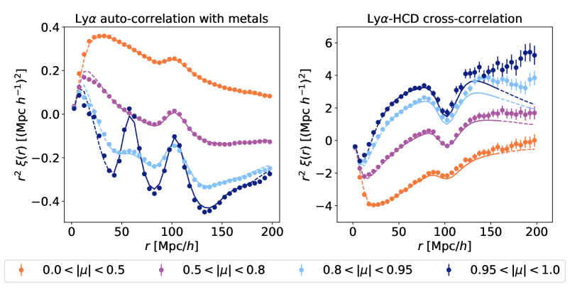
Figure 4: The correlation functions measured from 10 realisations of LyaCoLoRe combined, demonstrating the additional astrophysical effects that can be included in its skewers. The left panel shows the flux auto-correlation measured from skewers including metal absorption, from which we measure the metal absorber biases presented in Table 3. The right panel shows the Ly$\alpha$-HCD cross-correlation. The subtleties of this measurement — including the discrepancy at large-$r$ — are discussed in Appendix C. Note that the correlations presented here do not have any distortion from continuum-fitting and so should not be visually compared with the equivalent plots from recent BOSS/eBOSS data.

	bias $\times 10^{3}$
Absorber	LyaCoLoRe	BOSS DR12	eBOSS DR14
SiII (1260 Å)	$0$$-1.70\pm 0.04$	$-1.5\pm 1.2$	$-2.5\pm 1.3$
SiIII (1207 Å)	$-3.3$	$-3.3\pm 1.3$	$-8.2\pm 1.0$
SiII (1193 Å)	$0$$-3.28\pm 0.03$	$-3.5\pm 0.9$	$-4.6\pm 1.0$
SiII (1190 Å)	$0$$-4.55\pm 0.03$	$-4.4\pm 0.9$	$-5.1\pm 1.0$

Table 3: The biases of the metal absorbers used in our realisations of LyaColoRe, along with the values from BOSS DR12 [21] and eBOSS DR14 [22] for comparison. The bias of SiIII (1207) is held fixed to the DR12 value as the “bump” that it creates in the correlation function is at $r=21$ Mpc/$h$, below the minimum separation of 40 Mpc/$h$ used in our fits. The values from LyaColoRe are all within 1$\sigma$ of those from BOSS DR12, indicating that the absorption strengths used in our realisations (see Table 2) result in the correct levels of large-scale clustering.

We then compute the 3D auto-correlation from skewers of $F$ that include contributions from the additional absorption transitions in Table 2 (on top of Ly$\alpha$ absorption). The method used to do so is identical to that described for the 3D Ly$\alpha$ auto-correlation in § 4.2. We only include contributions from pixels that lie in the rest-frame wavelength range $[1040,1200]$ Å, and so we do not include any absorption from the Ly$\beta$ absorber as its rest-frame wavelength is below this range. As such, from here on we refer to the additional absorption transitions as “metals”. As in § 4, we measure correlations on each of our 10 realisations, and combine the measurements.

The measurement of the auto-correlation with metal absorbers is shown in the left panel of Figure 4. By comparison with Figure 3, the effect of including these metals in the skewers is clearly significant, particularly in the near-line of sight $0.95<|\mu|<1.0$ bin. Notably, we can clearly see a peak at approximately 55-60 Mpc/$h$ as a result of SiII (1190 Å) and SiII (1193 Å) absorption, as well as a peak at approximately 21 Mpc/$h$ from SiIII (1207 Å). This final peak is not included in our fit as it is below the minimum separation. Less visually obvious, but more important to the BAO analysis, is the effect of absorption from SiII (1260 Å), which causes a bump at 105 Mpc/$h$, very close to the BAO peak.

In our fit of this correlation, we model the effect of metal absorbers in the same way as in [22], summing contributions to the model power spectrum from each combination of pairs of absorbers. In Table 3, we show the biases for each of our metal absorbers, as well as the values from BOSS DR12 [21] and eBOSS DR14 [22] for comparison. The bias of SiIII (1207 Å) is held fixed to the DR12 value as the peak that it creates in the correlation function is at $r=21$ Mpc/$h$, below the minimum value used in our fits. The LyaColoRe values sit within 1$\sigma$ of those from BOSS DR12, demonstrating that the levels of clustering given by the absorption strengths in Table 2 are similar to those found in data. Of course, each absorption strength can be tuned further so that the bias of the relevant absorber more closely matches any given value.

6 Summary & conclusions

In this work we have presented LyaCoLoRe, a tool for creating mock Ly$\alpha$ forest datasets when used in conjunction with a Gaussian random field code such as CoLoRe. We first use CoLoRe to generate skewers from a Gaussian random field, avoiding the use of N-body or hydrodynamical simulations due to the limited volume and high computational cost of such methods. LyaCoLoRe is then able to transform the output into realistic skewers of transmitted flux fraction, with a number of properties defined by an automatic tuning process. The process is computationally efficient, making it suitable for generating large numbers of realisations of mocks with different input data and parameters.

We then demonstrate the effectiveness of LyaCoLoRe’s output, generating a number of skewers equivalent to approximately 30 realisations of DESI and measuring the Ly$\alpha$ auto- and Ly$\alpha$-QSO cross-correlations. Fitting these measurements with an appropriate model gives BAO peak positions that are consistent with the input cosmologies to within 0.2%, and certainly within the capabilities of an instrument such as DESI. In addition, the biases of the Ly$\alpha$ forest and of QSOs are shown to be very similar to those derived from BOSS DR12 data. As such, we conclude that the mock datasets generated by LyaCoLoRe are suitable for the BAO analyses of current and upcoming surveys such as eBOSS and DESI.

Finally, we demonstrate two additional capabilities of the LyaCoLoRe package in adding correlated high column density systems (HCDs) and additional absorption transitions to the skewers. We leave a full analysis on the impact of such features on a BAO analysis to a future work, but demonstrate that the HCDs are clustered approximately correctly on large scales, and that the additional transitions affect the Ly$\alpha$ auto-correlation in the expected manner.

Mock datasets such as those generated by LyaCoLoRe are of use to the BAO analyses of Ly$\alpha$ forest surveys in a number of ways. They are able to provide robust tests of analysis pipelines, while they can also help in assessing the impact of astrophysical effects — such as HCDs and additional absorption transitions — on BAO measurements. Finally, they can be used to provide evidence when making decisions regarding the planning of large surveys, such as in targeting and survey strategy. As such, we hope that LyaCoLoRe will be of use for Ly$\alpha$ BAO surveys both present and future.

Appendix A The quasar auto-correlation

We measure the quasar (QSO) auto-correlation on ten QSO catalogues from ten realisations of CoLoRe and combine our results. Correlations are computed as the weighted sum of pairs of QSOs in a grid of parallel and perpendicular separation bins. We divide the sky into HEALPix pixels, computing “data-data”, “data-random” and “random-random” correlations in each one using a random catalogue of QSOs. This random catalogue has the same number density distribution of QSOs as that in the mock data, and is generated by LyaColoRe. The different correlation types are then combined using the Landy-Szalay estimator [72], and the covariance is estimated via sub-sampling across HEALPix pixelisations of all 10 realisations (as described in § 4.2). As in § 4.2, all correlations are computed using picca. A Kaiser model [58] is then fitted to the measurement, leaving free parameters describing the location of the BAO peak and the QSO bias $b_{\delta,\mathrm{QSO}}$. As in § 4.3, we also leave free parameters describing the smoothing of the input power spectrum in the parallel and perpendicular directions. As in § 4.3, we fit only in the range $40<r\ [\mathrm{Mpc}/h]<160$ as the lognormal approximation begins to break down below this range. The resultant fit is very good in the fitted region, as shown in Figure 5. We measure a QSO bias of $3.57\pm 0.01$ at an effective redshift of $z=2.20$, consistent with the input value of $3.56$ to within $1\sigma$.

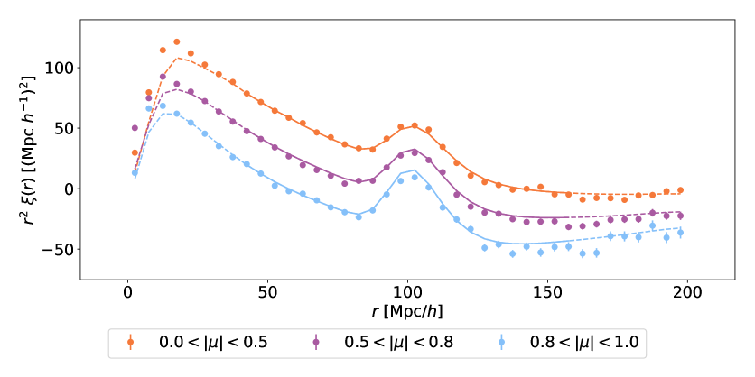
Figure 5: The auto-correlation of QSOs, as measured from ten realisations of CoLoRe. The fit is generally good in the fitted region, though the correlation on smaller scales than this is evidently too high.

Appendix B Redshift-space distortions: implementation details

As described in § 2.2.3, adding RSDs to our skewers requires the calculation of a matrix of weights $W_{ij}$ to map each skewer’s real-space cells $\tau^{x}_{j}$ to redshift-space cells $\tau^{s}_{i}$ via the matrix equation $\tau^{s}_{i}=W_{ij}\tau^{x}_{j}$. $W_{ij}$ is determined by representing each cell as a top-hat function in real space, mapping this profile into redshift space according to the choice of kernel $K$, and calculating the overlap with each redshift-space cell:

$$W_{ij}=\int_{s^{l}_{j}}^{s^{u}_{j}}P(s-x_{i}-v_{r,i}|T_{i},d_{i})\mathrm{d}s,$$ (B.1)

where ${s^{l}_{j}}$ and ${s^{u}_{j}}$ are the lower and upper boundaries of cell $j$ in redshift-space, and $P(x|T,d)$ describes the profile of the real-space cell when mapped into redshift space. $P(x|T,d)$ is dependent on the distance from the centre of the cell $x$, the temperature of the gas $T$ and the half-width of the cell $d$. The form of $P$ is determined by the choice of $K$ (defined in equation (2.6)):

$$P(x|T,d)=\frac{1}{2d}\int_{-d}^{d}K(x-y|T)\mathrm{d}y.$$ (B.2)

As such, in the case of $K$ chosen to be a Dirac delta function, the redshift-space cell is represented by a top-hat function (as it was in real space).

In order to account for thermal broadening when adding RSDs to our skewers, we must instead choose our kernel $K$ to be defined by

$$K(x|T)=\frac{1}{\sqrt{2\pi}\sigma_{v}(T)}\exp\bigg{(}-\frac{x^{2}}{2\sigma^{2}_{v}(T)}\bigg{)},$$ (B.3)

where $\sigma_{v}(T)$ is the thermal velocity dispersion, which we approximate as in [49] by

$$\sigma_{v}(T)=9.1\bigg{(}\frac{T}{10,000\rm{K}}\bigg{)}^{1/2}\ \mathrm{km\ s}^{-1},$$ (B.4)

for temperature $T(z,\textbf{x})=T_{0}(z)\rho(z,\textbf{x})^{\gamma(z)-1}$. As described in § 3, for the purposes of this work we fix $\gamma=1.5$. We also fix $T_{0}=10,000$ K in line with [16] and consistent with literature values [50, 49, 51]. Of course, these values can easily be updated to follow a more complex redshift dependence for any uses of LyaCoLoRe where thermal broadening effects become significant. Evaluating equation (B.2) for this choice of $K$ yields a cell profile in redshift space defined by

$$P(x|T,d)=\frac{1}{4d}\bigg{[}\mathrm{erf}\bigg{(}\frac{x+d}{\sqrt{2}\sigma_{v}(T)}\bigg{)}-\mathrm{erf}\bigg{(}\frac{x-d}{\sqrt{2}\sigma_{v}(T)}\bigg{)}\bigg{]},$$ (B.5)

and the matrix of weights can then be computed as per equation (B.1).

Appendix C The Ly$\alpha$-HCD cross-correlation

In Figure 4, we showed the cross-correlation between Ly$\alpha$ absorption and high column density systems (HCDs) from ten realisations of LyaCoLoRe, comparing it to a linear theory model similar to that used to describe the cross-correlation with quasars (QSOs). This model assumes that HCDs have the same clustering as dark matter halos, with a large-scale bias of approximately 2.0. However, in a QSO survey, HCDs are only detected when they are absorbing light from a background QSO, and this observational bias is not taken into account in our modelling. In this appendix, we propose that this bias results in an asymmetry in the measured correlation function. We present a qualitative description of this effect and explain our choice to use only HCDs detected far away from the QSO in Figure 4 in this context.

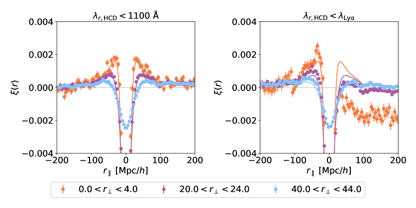
Figure 6: The Ly$\alpha$-HCD cross-correlation, plotted against $r_{\parallel}$ for different bins of $r_{\perp}$. The left panel shows the combined measurement from ten realisations using an HCD catalogue that only includes HCDS with rest-frame wavelength less than 1100 Å (as in the right panel of Figure 4). The right panel shows the correlation measured from one realisation when using an HCD catalogue that includes HCDs in the full rest-frame wavelength range, up to $\lambda_{\mathrm{Ly}\alpha}=1215.67$ Å. The solid lines in both panels show the same fitted correlation as in Figure 4: the joint fit of the Ly$\alpha$ auto-correlation and Ly$\alpha$-HCD cross-correlation from ten realisations of LyaCoLoRe.

In the left panel of Figure 6 we show the same measurement of the Ly$\alpha$-HCD cross-correlation as in the right panel of Figure 4, this time plotting the correlation against $r_{\parallel}$ in 3 narrow bins of $r_{\perp}$. The solid lines show the model obtained by fitting this measurement jointly with the Ly$\alpha$ auto-correlation. The model is generally able to fit the measurement well, though some small residuals remain at large $r_{\parallel}$. These are visible at large separations in the right panel of Figure 4, accentuated due to the factor of $r^{2}$ in that plot.

In the right panel of Figure 6 we plot the Ly$\alpha$-HCD cross-correlation measured on one realisation of LyaCoLoRe, this time using a full HCD catalogue (with no maximum rest-frame wavelength). The solid lines are the exact same lines as in the left panel. It is clear from this plot that there is a strong asymmetry in the data, and the model used to fit the data in the left panel does not fit this measurement well.

We propose that this asymmetry is a consequence of the observational bias that is inherently present in our HCD sample, and the dependence on the Ly$\alpha$-QSO cross-correlation that this induces. According to the density-QSO cross-correlation, a QSO $q$ will tend to have dense regions of gas around it. In relation to an HCD $X$ in $q$’s spectrum, these dense regions will be located at small $r_{\perp}$ and $r_{\parallel}\simeq r_{Xq}$, the distance between $X$ and $q$ (as $X$ is constrained to lie directly along the line of sight between $q$ and the observer). This preferential location of dense regions of gas will imprint a feature in the correlation between $X$ and neighbouring skewers of $\delta_{F}$ at these specific separations. Referring to the diagram in Figure 7, we can see that the cells of $\delta_{F}$ in Region 1 will tend to be significantly biased according to the Ly$\alpha$-QSO cross-correlation. Thus, we will see a feature in the correlation between HCD $X$ and its neighbouring skewer corresponding to this region. The shape of this feature is determined by the shape of the Ly$\alpha$-QSO cross-correlation at small $r_{t}$, as shown beneath Region 1. The cells in Region 2 will not be significantly affected by the presence of $q$, and so we would not expect to see a feature here.

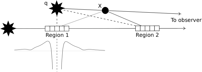
Figure 7: A diagram showing the geometry of the setup involved when measuring the Ly$\alpha$-HCD cross-correlation between two near-parallel skewers. Given the proximity of the QSO $q$ to “Region 1” of the lower skewer, we expect to measure biased values of $\delta_{F}$ for cells corresponding to that region. The cells’ values will tend to be reduced or boosted according to the Ly$\alpha$-QSO cross correlation, as indicated beneath “Region 1”. This biasing is then imprinted on the correlation between an HCD $X$ and the skewer.

Summing over HCD-pixel pairs in order to compute the full Ly$\alpha$-HCD cross-correlation will average out most of the signal, but a small, asymmetric residual will remain, as seen in the right panel of Figure 6. The contribution from each HCD will carry a similar signature but the signature will be centred at different values of $r_{\parallel}$ due to the different values of $r_{Xq}$ for each $X$-$q$ pair. Certainly though, the sign of $r_{Xq}$ will always be the same as an HCD is always less distant than its host QSO. Using picca’s definition of the sign of $r_{\parallel}$, this means that $r_{Xq}>0$ for all $X$ and $q$. As a result, we will see a reduction of the Ly$\alpha$-HCD cross-correlation for all $r_{\parallel}>0$, due to the strong reduction in $\delta_{F}$ at the centre of regions such as Region 1 in Figure 7. This is only apparent for $r_{\perp}$ small as the reduced area shown in Figure 7 is narrow. We also see a secondary effect: a boost in the Ly$\alpha$-HCD cross-correlation for small, negative $r_{\parallel}$. This is a result of the small boost in $\delta_{F}$ on the right-hand side of Region 1 in Figure 7, which appears at $r_{\parallel}<0$ for HCDs that are very close to their host QSOs. This effect extends to larger values of $r_{\perp}$ due to the greater width of the boosted area (relative to that which is reduced).

Whilst interesting, these effects are very small. In order to assess their visibility in current/future studies, we would need to carry out tests using a more realistic mock dataset. This would involve using the entire data reduction pipeline — including continuum fitting and the use of a distortion matrix — and is beyond the scope of this work. As an approximate comparison, we observe that the size of the deviation of points in the $0.0<r_{\perp}<4.0$ bin in the right panel of Figure 6 is approximately an order of magnitude smaller than the size of the error bars in the uppermost two panels of Figure 2 of [66].

Making such an extreme cut in rest-frame wavelength greatly reduces the number of HCDs in our catalogue. In this work we use approximately 30 times the number of skewers as DESI will have, and so this reduction does not cause us any concern. For studies from real surveys, however, maximising the scientific value of their data will be of much greater importance. As such, we would recommend the development of a new model to account for the effects described above using the measured Ly$\alpha$-QSO cross-correlation. Alternatively, a catalogue of random HCDs, uncorrelated with the Ly$\alpha$ forest, could be generated and used to quantify these effects before accounting for them appropriately. Either way, further tests are needed in order to understand more fully the effect described in this Appendix, particularly if new modelling is required for future Ly$\alpha$-HCD cross-correlation measurements.

References

- [1] A. G. Riess, A. V. Filippenko, P. Challis, A. Clocchiatti, A. Diercks, P. M. Garnavich et al., Observational Evidence from Supernovae for an Accelerating Universe and a Cosmological Constant, AJ 116 (1998) 1009 [astro-ph/9805201].
- [2] S. Perlmutter, G. Aldering, G. Goldhaber, R. A. Knop, P. Nugent, P. G. Castro et al., Measurements of and from 42 High-Redshift Supernovae, ApJ 517 (1999) 565 [astro-ph/9812133].
- [3] P. J. E. Peebles and J. T. Yu, Primeval Adiabatic Perturbation in an Expanding Universe, ApJ 162 (1970) 815.
- [4] D. J. Eisenstein, I. Zehavi, D. W. Hogg, R. Scoccimarro, M. R. Blanton, R. C. Nichol et al., Detection of the Baryon Acoustic Peak in the Large-Scale Correlation Function of SDSS Luminous Red Galaxies, ApJ 633 (2005) 560 [astro-ph/0501171].
- [5] S. Cole, W. J. Percival, J. A. Peacock, P. Norberg, C. M. Baugh, C. S. Frenk et al., The 2dF Galaxy Redshift Survey: power-spectrum analysis of the final data set and cosmological implications, MNRAS 362 (2005) 505 [astro-ph/0501174].
- [6] W. J. Percival, B. A. Reid, D. J. Eisenstein, N. A. Bahcall, T. Budavari, J. A. Frieman et al., Baryon acoustic oscillations in the Sloan Digital Sky Survey Data Release 7 galaxy sample, MNRAS 401 (2010) 2148 [0907.1660].
- [7] F. Beutler, C. Blake, M. Colless, D. H. Jones, L. Staveley-Smith, L. Campbell et al., The 6dF Galaxy Survey: baryon acoustic oscillations and the local Hubble constant, MNRAS 416 (2011) 3017 [1106.3366].
- [8] C. Blake, E. A. Kazin, F. Beutler, T. M. Davis, D. Parkinson, S. Brough et al., The WiggleZ Dark Energy Survey: mapping the distance-redshift relation with baryon acoustic oscillations, MNRAS 418 (2011) 1707 [1108.2635].
- [9] S. Alam, M. Ata, S. Bailey, F. Beutler, D. Bizyaev, J. A. Blazek et al., The clustering of galaxies in the completed SDSS-III Baryon Oscillation Spectroscopic Survey: cosmological analysis of the DR12 galaxy sample, MNRAS 470 (2017) 2617 [1607.03155].
- [10] M. Ata, F. Baumgarten, J. Bautista, F. Beutler, D. Bizyaev, M. R. Blanton et al., The clustering of the SDSS-IV extended Baryon Oscillation Spectroscopic Survey DR14 quasar sample: first measurement of baryon acoustic oscillations between redshift 0.8 and 2.2, MNRAS 473 (2018) 4773 [1705.06373].
- [11] H. G. Bi, G. Boerner and Y. Chu, An alternative model for the Ly-alpha absorption forest., A&A 266 (1992) 1.
- [12] R. Cen, J. Miralda-Escudé, J. P. Ostriker and M. Rauch, Gravitational Collapse of Small-Scale Structure as the Origin of the Lyman-Alpha Forest, ApJ 437 (1994) L9 [astro-ph/9409017].
- [13] P. Petitjean, J. P. Mueket and R. E. Kates, The Ly forest at low redshift: tracing the dark matter filaments., A&A 295 (1995) L9 [astro-ph/9502100].
- [14] J. Miralda-Escudé, R. Cen, J. P. Ostriker and M. Rauch, The Ly alpha Forest from Gravitational Collapse in the Cold Dark Matter + Lambda Model, ApJ 471 (1996) 582 [astro-ph/9511013].
- [15] P. McDonald and D. J. Eisenstein, Dark energy and curvature from a future baryonic acoustic oscillation survey using the Lyman- forest, Phys.Rev.D 76 (2007) 063009 [astro-ph/0607122].
- [16] A. Slosar, A. Font-Ribera, M. M. Pieri, J. Rich, J.-M. Le Goff, É. Aubourg et al., The Lyman- forest in three dimensions: measurements of large scale flux correlations from BOSS 1st-year data, JCAP 2011 (2011) 001 [1104.5244].
- [17] N. G. Busca, T. Delubac, J. Rich, S. Bailey, A. Font-Ribera, D. Kirkby et al., Baryon acoustic oscillations in the Ly forest of BOSS quasars, A&A 552 (2013) A96 [1211.2616].
- [18] A. Slosar, V. Iršič, D. Kirkby, S. Bailey, N. G. Busca, T. Delubac et al., Measurement of baryon acoustic oscillations in the Lyman- forest fluctuations in BOSS data release 9, JCAP 2013 (2013) 026 [1301.3459].
- [19] D. Kirkby, D. Margala, A. Slosar, S. Bailey, N. G. Busca, T. Delubac et al., Fitting methods for baryon acoustic oscillations in the Lyman- forest fluctuations in BOSS data release 9, JCAP 2013 (2013) 024 [1301.3456].
- [20] T. Delubac, J. E. Bautista, N. G. Busca, J. Rich, D. Kirkby, S. Bailey et al., Baryon acoustic oscillations in the Ly forest of BOSS DR11 quasars, A&A 574 (2015) A59 [1404.1801].
- [21] J. E. Bautista, N. G. Busca, J. Guy, J. Rich, M. Blomqvist, H. du Mas des Bourboux et al., Measurement of baryon acoustic oscillation correlations at z = 2.3 with SDSS DR12 Ly-Forests, A&A 603 (2017) A12 [1702.00176].
- [22] V. de Sainte Agathe, C. Balland, H. du Mas des Bourboux, N. G. Busca, M. Blomqvist, J. Guy et al., Baryon acoustic oscillations at z = 2.34 from the correlations of Ly absorption in eBOSS DR14, A&A 629 (2019) A85 [1904.03400].
- [23] A. Font-Ribera, E. Arnau, J. Miralda-Escudé, E. Rollinde, J. Brinkmann, J. R. Brownstein et al., The large-scale quasar-Lyman forest cross-correlation from BOSS, JCAP 2013 (2013) 018 [1303.1937].
- [24] A. Font-Ribera, D. Kirkby, N. Busca, J. Miralda-Escudé, N. P. Ross, A. Slosar et al., Quasar-Lyman forest cross-correlation from BOSS DR11: Baryon Acoustic Oscillations, JCAP 2014 (2014) 027 [1311.1767].
- [25] H. du Mas des Bourboux, J.-M. Le Goff, M. Blomqvist, N. G. Busca, J. Guy, J. Rich et al., Baryon acoustic oscillations from the complete SDSS-III Ly-quasar cross-correlation function at z = 2.4, A&A 608 (2017) A130 [1708.02225].
- [26] M. Blomqvist, H. du Mas des Bourboux, N. G. Busca, V. de Sainte Agathe, J. Rich, C. Balland et al., Baryon acoustic oscillations from the cross-correlation of Ly absorption and quasars in eBOSS DR14, A&A 629 (2019) A86 [1904.03430].
- [27] DESI Collaboration, A. Aghamousa, J. Aguilar, S. Ahlen, S. Alam, L. E. Allen et al., The DESI Experiment Part I: Science,Targeting, and Survey Design, arXiv e-prints (2016) arXiv:1611.00036 [1611.00036].
- [28] J. M. Le Goff, C. Magneville, E. Rollinde, S. Peirani, P. Petitjean, C. Pichon et al., Simulations of BAO reconstruction with a quasar Ly- survey, A&A 534 (2011) A135 [1107.4233].
- [29] A. Font-Ribera, P. McDonald and J. Miralda-Escudé, Generating mock data sets for large-scale Lyman- forest correlation measurements, JCAP 2012 (2012) 001 [1108.5606].
- [30] J. E. Bautista, S. Bailey, A. Font-Ribera, M. M. Pieri, N. G. Busca, J. Miralda-Escudé et al., Mock Quasar-Lyman- forest data-sets for the SDSS-III Baryon Oscillation Spectroscopic Survey, JCAP 2015 (2015) 060 [1412.0658].
- [31] P. Coles and B. Jones, A lognormal model for the cosmological mass distribution., MNRAS 248 (1991) 1.
- [32] H. Bi and A. F. Davidsen, Evolution of Structure in the Intergalactic Medium and the Nature of the Ly Forest, ApJ 479 (1997) 523 [astro-ph/9611062].
- [33] F. Bernardeau, S. Colombi, E. Gaztañaga and R. Scoccimarro, Large-scale structure of the Universe and cosmological perturbation theory, physrep 367 (2002) 1 [astro-ph/0112551].
- [34] S. Tassev, M. Zaldarriaga and D. J. Eisenstein, Solving large scale structure in ten easy steps with COLA, JCAP 2013 (2013) 036 [1301.0322].
- [35] R. A. C. Croft, D. H. Weinberg, N. Katz and L. Hernquist, Recovery of the Power Spectrum of Mass Fluctuations from Observations of the Ly Forest, ApJ 495 (1998) 44 [astro-ph/9708018].
- [36] V. Iršič and M. McQuinn, Absorber Model: the Halo-like model for the Lyman- forest, JCAP 2018 (2018) 026 [1801.02671].
- [37] D. Alonso and collaborators, CoLoRe: Cosmological lognormal realisations, in preparation, 2020.
- [38] M. Walther, J. F. Hennawi, H. Hiss, J. Oñorbe, K.-G. Lee, A. Rorai et al., A New Precision Measurement of the Small-scale Line-of-sight Power Spectrum of the Ly Forest, ApJ 852 (2018) 22 [1709.07354].
- [39] P. McDonald, U. Seljak, S. Burles, D. J. Schlegel, D. H. Weinberg, R. Cen et al., The Ly Forest Power Spectrum from the Sloan Digital Sky Survey, ApJS 163 (2006) 80 [astro-ph/0405013].
- [40] L. Hui and N. Y. Gnedin, Equation of state of the photoionized intergalactic medium, MNRAS 292 (1997) 27 [astro-ph/9612232].
- [41] L. Hui, N. Y. Gnedin and Y. Zhang, The Statistics of Density Peaks and the Column Density Distribution of the Ly Forest, ApJ 486 (1997) 599 [astro-ph/9608157].
- [42] J. E. Gunn and B. A. Peterson, On the Density of Neutral Hydrogen in Intergalactic Space., ApJ 142 (1965) 1633.
- [43] P. McDonald, Toward a Measurement of the Cosmological Geometry at z ~2: Predicting Ly Forest Correlation in Three Dimensions and the Potential of Future Data Sets, ApJ 585 (2003) 34 [astro-ph/0108064].
- [44] N. Palanque-Delabrouille, C. Yèche, A. Borde, J.-M. Le Goff, G. Rossi, M. Viel et al., The one-dimensional Ly forest power spectrum from BOSS, A&A 559 (2013) A85 [1306.5896].
- [45] G. D. Becker, P. C. Hewett, G. Worseck and J. X. Prochaska, A refined measurement of the mean transmitted flux in the Ly forest over 2 < z < 5 using composite quasar spectra, MNRAS 430 (2013) 2067 [1208.2584].
- [46] M. McQuinn and M. White, On estimating Ly forest correlations between multiple sightlines, MNRAS 415 (2011) 2257 [1102.1752].
- [47] F. James and M. Roos, Minuit - a system for function minimization and analysis of the parameter errors and correlations, Computer Physics Communications 10 (1975) 343.
- [48] U. Seljak, Bias, redshift space distortions and primordial nongaussianity of nonlinear transformations: application to Ly- forest, JCAP 2012 (2012) 004 [1201.0594].
- [49] P. McDonald, J. Miralda-Escudé, M. Rauch, W. L. W. Sargent, T. A. Barlow and R. Cen, A Measurement of the Temperature-Density Relation in the Intergalactic Medium Using a New Ly Absorption-Line Fitting Method, ApJ 562 (2001) 52 [astro-ph/0005553].
- [50] M. Ricotti, N. Y. Gnedin and J. M. Shull, The Evolution of the Effective Equation of State of the Intergalactic Medium, ApJ 534 (2000) 41 [astro-ph/9906413].
- [51] H. Hiss, M. Walther, J. F. Hennawi, J. Oñorbe, J. M. O’Meara, A. Rorai et al., A New Measurement of the Temperature-density Relation of the IGM from Voigt Profile Fitting, ApJ 865 (2018) 42 [1710.00700].
- [52] A. Lewis, A. Challinor and A. Lasenby, Efficient Computation of Cosmic Microwave Background Anisotropies in Closed Friedmann-Robertson-Walker Models, ApJ 538 (2000) 473 [astro-ph/9911177].
- [53] Planck Collaboration, P. A. R. Ade, N. Aghanim, M. Arnaud, M. Ashdown, J. Aumont et al., Planck 2015 results. XIII. Cosmological parameters, A&A 594 (2016) A13 [1502.01589].
- [54] N. Palanque-Delabrouille, C. Magneville, C. Yèche, I. Pâris, P. Petitjean, E. Burtin et al., The extended Baryon Oscillation Spectroscopic Survey: Variability selection and quasar luminosity function, A&A 587 (2016) A41 [1509.05607].
- [55] S. Gontcho A Gontcho, J. Miralda-Escudé, A. Font-Ribera, M. Blomqvist, N. G. Busca and J. Rich, Quasar - CIV forest cross-correlation with SDSS DR12, MNRAS 480 (2018) 610 [1712.09886].
- [56] P. Laurent, J.-M. Le Goff, E. Burtin, J.-C. Hamilton, D. W. Hogg, A. Myers et al., A 14 h-3 Gpc3 study of cosmic homogeneity using BOSS DR12 quasar sample, JCAP 2016 (2016) 060 [1602.09010].
- [57] K. M. Górski, E. Hivon, A. J. Banday, B. D. Wand elt, F. K. Hansen, M. Reinecke et al., HEALPix: A Framework for High-Resolution Discretization and Fast Analysis of Data Distributed on the Sphere, ApJ 622 (2005) 759 [astro-ph/0409513].
- [58] N. Kaiser, Clustering in real space and in redshift space, MNRAS 227 (1987) 1.
- [59] A. M. Wolfe, D. A. Turnshek, H. E. Smith and R. D. Cohen, Damped Lyman-Alpha Absorption by Disk Galaxies with Large Redshifts. I. The Lick Survey, ApJS 61 (1986) 249.
- [60] A. Font-Ribera and J. Miralda-Escudé, The effect of high column density systems on the measurement of the Lyman- forest correlation function, JCAP 2012 (2012) 028 [1205.2018].
- [61] K. K. Rogers, S. Bird, H. V. Peiris, A. Pontzen, A. Font-Ribera and B. Leistedt, Correlations in the three-dimensional Lyman-alpha forest contaminated by high column density absorbers, MNRAS 476 (2018) 3716 [1711.06275].
- [62] M. Pettini, L. J. Smith, D. L. King and R. W. Hunstead, The Metallicity of High-Redshift Galaxies: The Abundance of Zinc in 34 Damped Ly Systems from z = 0.7 to 3.4, ApJ 486 (1997) 665 [astro-ph/9704102].
- [63] J. X. Prochaska, R. B. C. Henry, J. M. O’Meara, D. Tytler, A. M. Wolfe, D. Kirkman et al., The UCSD HIRES/Keck I Damped Ly Abundance Database. IV. Probing Galactic Enrichment Histories with Nitrogen, PASP 114 (2002) 933 [astro-ph/0206296].
- [64] H. Padmanabhan, T. R. Choudhury and A. Refregier, Modelling the cosmic neutral hydrogen from DLAs and 21-cm observations, MNRAS 458 (2016) 781 [1505.00008].
- [65] I. Pérez-Ràfols, J. Miralda-Escudé, A. Arinyo-i-Prats, A. Font-Ribera and L. Mas-Ribas, The cosmological bias factor of damped Lyman alpha systems: dependence on metal line strength, MNRAS 480 (2018) 4702 [1805.00943].
- [66] I. Pérez-Ràfols, A. Font-Ribera, J. Miralda-Escudé, M. Blomqvist, S. Bird, N. Busca et al., The SDSS-DR12 large-scale cross-correlation of damped Lyman alpha systems with the Lyman alpha forest, MNRAS 473 (2018) 3019 [1709.00889].
- [67] J. X. Prochaska, N. Tejos, cwotta, jnburchett, M. Fumagalli, marijana777 et al., pyigm/pyigm: Initial release for publications, Nov., 2017. 10.5281/zenodo.1045480.
- [68] J. X. Prochaska, P. Madau, J. M. O’Meara and M. Fumagalli, Towards a unified description of the intergalactic medium at redshift z 2.5, MNRAS 438 (2014) 476 [1310.0052].
- [69] M. M. Pieri, M. J. Mortonson, S. Frank, N. Crighton, D. H. Weinberg, K.-G. Lee et al., Probing the circumgalactic medium at high-redshift using composite BOSS spectra of strong Lyman forest absorbers, MNRAS 441 (2014) 1718 [1309.6768].
- [70] M. Blomqvist, M. M. Pieri, H. du Mas des Bourboux, N. G. Busca, A. Slosar, J. E. Bautista et al., The triply-ionized carbon forest from eBOSS: cosmological correlations with quasars in SDSS-IV DR14, JCAP 2018 (2018) 029 [1801.01852].
- [71] H. du Mas des Bourboux, K. S. Dawson, N. G. Busca, M. Blomqvist, V. de Sainte Agathe, C. Balland et al., The Extended Baryon Oscillation Spectroscopic Survey: Measuring the Cross-correlation between the Mg II Flux Transmission Field and Quasars and Galaxies at z = 0.59, ApJ 878 (2019) 47 [1901.01950].
- [72] S. D. Landy and A. S. Szalay, Bias and Variance of Angular Correlation Functions, ApJ 412 (1993) 64.