The disc–like host galaxies of radio loud Narrow-Line Seyfert 1s

Abstract

Until recently, relativistic jets were ubiquitously found to be launched from giant elliptical galaxies. However, the detection by the Fermi–LAT of $\gamma-$ray emission from radio–loud narrow–line Seyfert 1 (RL–NLSy1) galaxies raised doubts on this relation. Here, we morphologically characterize a sample of 29 RL–NLSy1s (including 12 $\gamma-$emitters, $\gamma-$NLSy1s) in order to find clues on the conditions needed by AGN to produce relativistic jets. We use deep near-infrared images from the Nordic Optical Telescope and the ESO VLT to analyze the surface brightness distribution of the galaxies in the sample. We detected 72% of the hosts (24% classified as $\gamma-$NLSy1s). Although we cannot rule out that some RL–NLSy1s are hosted by dispersion supported systems, our findings strongly indicate that RL–NLSy1s hosts are preferentially disc galaxies. 52% of the resolved hosts (77% non $\gamma-$emitters and 20% $\gamma-$emitters) show bars with morphological properties (long and weak) consistent with models that promote gas inflows, which might trigger nuclear activity. The extremely red bulges of the $\gamma-$NLSy1s, and features that suggest minor mergers in 75% of their hosts, might hint to the necessary conditions for $\gamma-$rays to be produced. Among the features that suggest mergers in our sample, we find 6 galaxies that show offset stellar bulges with respect to their AGN. When we plot the nuclear versus the bulge magnitude, RL–NLSy1s locate in the low–luminosity end of flat spectrum radio quasars (FSRQs), suggesting a similar accretion mode between these two AGN types.

1 Introduction

Because of the tight empirical relations observed between the black hole mass and different properties of its host galaxy bulge (Magorrian et al., 1998; Gebhardt et al., 2000; Ferrarese & Merritt, 2000; Tremaine et al., 2002; Gültekin et al., 2009), it is now widely accepted that there is a strong connection between the supermassive black holes (SMBHs) and their host galaxies. The link between the black hole and its host galaxy is thought to be the AGN activity, through feedback processes (either positive or negative; for a review see Fabian, 2012; Heckman & Best, 2014). If this is the case, then, we can assume that the more powerful the AGN, the stronger the influence on its host galaxy. In fact, a study by Olguín-Iglesias et al. 2016 (performed on $\mathrm{0.3<z<1.0}$, strongly beamed AGN, whose relativistic jets point towards the Earth, i.e. blazars) suggests that the AGN impact their hosts (either by suppression or triggering of star formation) in a magnitude that is proportional to the jet power.

Until recently, powerful relativistic radio jets were virtually only found to be hosted in elliptical galaxies (e.g. Stickel et al., 1991; Kotilainen et al., 1998b, a; Scarpa et al., 2000; Urry et al., 2000; Kotilainen et al., 2005; Hyvönen et al., 2007; Olguín-Iglesias et al., 2016), which helped develop ideas on how jets, supermassive black holes and their host galaxies evolve. However, recently, a few studies report on blazar–like disc hosts, that is to say, with fully developed relativistic jets, capable of emitting $\gamma-$ray photons (Kotilainen et al., 2016; Olguín-Iglesias et al., 2017, and probably León Tavares et al. 2014). These blazar–like disc galaxies, constitute a peculiar type of AGN known as Narrow–line Seyfert 1s (NLSy1s), characterized by narrower Balmer lines full width at half maximum ($\mathrm{FWHM(H\beta)<2000\ km\ s^{-1}}$) than in normal Seyferts, flux ratios $\mathrm{[OIII]/H\beta<3}$, strong optical FeII lines (FeII bump) and a soft X-ray excess (Osterbrock & Pogge, 1985; Orban de Xivry et al., 2011). Based on the full width at half maximum (FWHM) of their Broad Line Region (BLR) lines and the continuum luminosity (Kaspi et al., 2000), their central black holes masses ($\mathrm{M_{BH}}$) are estimated to range from $\mathrm{\sim 10^{6}M_{\odot}}$ to $\mathrm{\sim 10^{7}M_{\odot}}$ (Mathur et al., 2012a) and thus, their accretion rates are thought to be close to the Eddington limit. A small fraction has been found to be radio loud (RL, 7%, Komossa et al., 2006) and among them, a smaller fraction (so far, 15 galaxies), are the above-mentioned $\gamma-$ray emitters NLSy1s (hereafter, $\gamma-$NLSy1s).

Table 1: Main properties of the RL–NLSy1s analysed in this work and observations log.

Source	Name	z	RA	DEC	UT Date	Scale	Seeing	Exposure time
						kpc/”	(arcsec)	(s)
(1)	(2)	(3)	(4)	(5)	(6)	(7)	(8)	(9)
0321$+$340γ	1H 0323$+$342	0.061	03:24:41.1	$+$34:10:46.0	23-Jan-13	1.177	1.00/1.00	1800/1800
0846$+$513γ	SBS 0846+513	0.580	08:49:58.0	$+$51:08:29.0	14-Feb-16	6.579	0.65/0.67	3000/2700
0929+533γ	J093241+53063	0.590	09:32:41.1	+53:06:33.3	30-Mar-18	6.633	-/0.77	-/4356
0948$+$002γ	PMN J0948$+$0022	0.585	09:48:57.3	$+$00:22:26.0	21-Feb-14	6.606	0.73/0.77	4950/4890
0955+32γ	J095820+322401	0.530	09:58:20.9	$+$32:24:01.6	31-Mar-18	6.293	-/0.78	-/3600
1102+2239	FBQS J1102+2239	0.453	11:02:23.4	$+$22:39:20.7	14-Feb-14	5.781	-/0.79	-/2700
1159$-$011	IRAS 11598$-$0112	0.150	12:02:26.8	$-$01:29:15.0	13-Feb-16	2.614	0.79/0.82	2280/900
1200$-$004	RXSJ12002$-$0046	0.179	12:00:14.1	$-$00:46:39.0	14-Feb-16	3.021	0.64/0.67	1080/960
1217$+$654	J12176$+$6546	0.307	12:17:40.4	$+$65:46:50.0	13-Feb-16	4.526	0.94/0.79	2160/2160
1219$-$044γ	4C$+$04.42	0.996	12:22:22.5	$+$04:13:16.0	29-Mar-14	8.001	0.80/0.84	3650/2160
1227$+$321	RXSJ12278$+$3215	0.137	12:27:49.2	$+$32:14:59.0	14-Feb-16	2.423	0.70/0.67	930/930
1246+0238γ	SDSS J124634.65+023809	0.362	12:46:34.6	02:38:09.1	12-Aug-17	5.048	-/0.80	-/3480
1337$+$600	J13374$+$6005	0.234	13:37:24.4	$+$60:05:41.0	13-Feb-16	3.722	0.73/0.72	2160/2160
1403$+$022	J14033$+$0222	0.250	14:03:22.1	$+$02:22:33.0	14-Feb-16	3.910	0.66/0.59	1380/1080
1421+3855γ	J142106+385522γ	0.490	14:21:06.0	+38:55:22.5	14-Mar-18	6.038	-/0.75	-/2754
1441$-$476γ	B3 1441$+$476	0.705	14:43:18.5	$+$47:25:57.0	24-Apr-16	7.166	-/0.80	-/2700
1450+591	J14506+5919	0.202	14:50:42.0	$+$59:19:37	22-May-14	3.325	0.82/0.82	900/1020
1502$+$036${}^{\gamma\ *}$	PKS 1502$+$036	0.409	15:05:06.5	$+$03:26:31.0	04-Apr-13	5.446	0.80/0.82	920/280
1517$+$520	SBS 1517$+$520	0.371	15:18:32.9	$+$51:54:57.0	14-Feb-16	5.128	0.63/0.67	1140/960
1546$+$353	B2 1546$+$35A	0.479	15:48:17.9	$+$35:11:28.0	13-Feb-16	5.964	0.68/0.74	2160/2340
1629$+$400	J16290$+$4007	0.272	16:29:01.3	$+$40:08:00.0	13-Feb-16	4.157	0.63/0.62	2160/2160
1633$+$471	RXSJ16333$+$4718	0.116	16:33:23.5	$+$47:19:00.0	14-Feb-16	2.101	0.62/0.63	1260/1050
1640$+$534	2E 1640$+$5345	0.140	16:42:00.6	$+$53:39:51.0	14-Feb-16	2.468	0.60/0.64	1200/1080
1641$+$345	J16410$+$3454	0.164	16:41:00.1	$+$34:54:52.0	14-Feb-16	2.814	0.62/0.70	1320/1800
1644$+$261γ	FBQS J1644+2619	0.145	16:44:42.5	$+$26:19:13.0	01-May-15	2.541	0.75/0.63	2550/2160
1702+457	B31702+457	0.060	17:03:30.3	$+$45:40:47.2	21-Jun-16	1.159	-/0.79	-/945
1722$+$565	J17221$+$5654	0.426	17:22:06.0	$+$56:54:51.0	13-Feb-16	5.579	0.62/0.60	2040/2040
2004$-$447${}^{\gamma\ *}$	PKS 2004$-$447	0.240	20:07:55.2	$-$44:34:44.0	16-Apr-13	3.793	0.40/0.45	600/110
2245$-$174	IRAS 22453$-$1744	0.117	22:48:04.2	$-$17:28:30.0	14-Feb-16	2.116	1.44/-	1260/-

Columns: (1) and (2) give the designation and name of the source; (3) the redshift of the object; (4) and (5) the J2000 right ascension and declination of the source; (6) the observation date; (7) the target scale; (8) the seeing during the observation in J– and Ks–band, respectively, and (9) the total exposure time for J– and Ks–band, respectively.
^∗ Galaxies observed using the ISAAC on the ESO/VLT
^γ $\gamma-$ray emitting NLSy1 galaxies

RL–NLSy1s (including $\gamma-$NLSy1s), are excellent laboratories to study the mechanisms that make AGN able to launch and collimate fully developed relativistic outflows at a likely early evolutionary stage. Thus, in this study, we characterize a sample of RL–NLSy1s (including 12 $\gamma-$NLSys detected so far) with the aim of determining the properties of their host galaxies that could shed some light on the necessary conditions and mechanisms to generate the relativistic jet phenomenon.

This paper is organized as follows. In Section 2, we present the sample and observations. In Section 3 we explain the data reduction and the methodology of the analysis. In Section 4 we discuss the results and compare them with previous studies. Finally, in Section 6, we summarize our findings. All quantitative values given in this paper are based on a cosmology with $\mathrm{H_{0}=70kms^{-1}Mpc^{-1}}$, $\mathrm{\Omega_{m}=0.3}$, and $\mathrm{\Omega_{\Lambda}=0.7}$.

2 Sample and observations

The initial sample consists of 12 $\gamma-$ray emitting NLSy1s (Abdo et al., 2009a, b; Foschini, 2011; D’Ammando et al., 2012; D’Ammando et al., 2015; Liao et al., 2015; Yao et al., 2015; Paliya et al., 2018). Given that $\gamma-$NLSy1s are also radio loud (RL), we expanded this sample by imaging the host galaxies of 17 radio–loud, but not $\gamma-$ray emitting NLSy1s, as a comparison sample. These galaxies are all observable from the northern hemisphere, have redshifts $\mathrm{z<0.5}$ and radio–loudness ($\mathrm{RL\equiv f_{\nu,4.85GHz}/f_{\nu,B},RL>31}$).

The observations were conducted using two different telescopes, the Nordic Optical Telescope (NOT), using the near–infrared camera NOTcam (pixel scale = $0.234^{\prime\prime}$/pixel and field-of-view FOV$=4^{\prime}\times 4^{\prime}$) and the ESO very large telescope (VLT), using its infrared spectrometer and array camera (ISAAC, pixel scale =$0.148^{\prime\prime}$ and FOV = $152^{\prime\prime}\times 152^{\prime\prime}$ Moorwood et al., 1998), depending on the declination of each galaxy. On the other hand the RL-NLSy1s (but not $\gamma-$ray emitters) in the sample were observed with the NOT telescope, between 2013 January 23 and 2016 February 14 using the NOTcam.

As is usual in the near–infrared, all the targets in the sample were imaged using a jitter procedure to obtain a set of offset frames with respect to the initial position. Each target was observed in J– and/or K–bands, during an average exposure time of $\mathrm{EXPTIME\approx 1800s}$, and an average seeing $\sim 0.75$arcsec (see table 1).

3 Data reduction and analysis

3.1 Data reduction

The images of the galaxies in the sample observed with the NOT were reduced using the NOTCam script for IRAF REDUCE . This script takes the consequtive dithered images, corrects for flatfield, interpolates over bad pixels, and makes a sky template that is subtracted from each image. The images are then registered based on interactively selected stars (and RA/DEC header keywords) and combined to obtain the final reduced image. For the images observed with the ISAAC a similar procedure was followed. A flat frame was derived from the twilight images and a sky image was obtained by median filtering the individual frames in the stack. The individual frames were then aligned using bright stars as reference points in the field and combined to produce the final reduced co–added image (see Olguín-Iglesias et al., 2016, for more details). The photometric calibration was performed by using the field stars in our images with the magnitudes reported by 2MASS (Skrutskie et al., 2006).

3.2 Photometric decomposition

The 2D light distribution of the reduced images is modeled using the image analysis algorithm GALFIT (Peng et al., 2011). The different components of a galaxy are described using different analytical functions. For bulges and possible bars in the host galaxies of the sample, we use the Sérsic profile, which functional form is:

$$\mathrm{\Sigma(r)=\Sigma_{e}exp\left[-\kappa\left(\left(\frac{r}{r_{e}}\right)^{1/n}-1\right)\right]}$$ (1)

where $\mathrm{\Sigma_{e}}$ is the surface brightness of the pixel in the effective radius ($\mathrm{r_{e}}$, radius where half of the total flux is concentrated). The parameter n (the Sérsic index) is often referred to as a concentration parameter and the variable $\mathrm{\kappa}$ is coupled to it.

We also use the exponential function, since it describes well the radial behavior of galactic discs. Although, the exponential function is a special case of the Sérsic profile (when $\mathrm{n=1}$), nomenclature–wise, we use it when the component to fit is a disc, otherwise we use the Sérsic profile with $\mathrm{n=1}$. Its functional form is:

$$\mathrm{\Sigma(r)=\Sigma_{0}exp\left(-\frac{r}{r_{s}}\right)}$$ (2)

where $\mathrm{\Sigma(r)}$ is the surface brightness at a radius r, $\mathrm{\Sigma_{0}}$ is the surface brightness at the center of the target and $\mathrm{r_{s}}$ is the scale length of the disc.

The sky background is also modeled. We use a simple flat plane that can be tilted in x and y direction. Finally, the nuclear emission due to the powerful AGN of the galaxies of the sample is fitted using a modeled point spread function (PSF).

3.2.1 PSF modeling

In most cases, the PSF modeling, only consists on subtracting a bright non–saturated star close to the target and removing its background. However, it is not always possible to get a suitable star in the field of view (FOV). In the case where only saturated or faint stars are found, the following procedure is implemented:

First, we identify the stars in the FOV. Then, we select, preferentially, the stars with no sources within $\sim$7” radius and more than $\sim$10” away from the border of the FOV. The selected stars are centered in 50”$\times$50” boxes, where all extra sources are masked out by means of the segmentation image process of SExtractor (Bertin & Arnouts, 1996). The wings of the PSF are modeled by fitting a saturated star with a number of exponential and Gaussian functions (top panel Figure 1). The core of the PSF is modeled by using another star (in this case, it is important not to be saturated) with Gaussian functions and the previously generated wings model (bottom panel Figure 1). The magnitude difference between the saturated and non–saturated stars is important, since there must be an overlap in order to match the wings and core models. The resultant model is tested by fitting random stars in the FOV.

In order to take into account the image PSF in the modeling of the galaxies, we convolved our PSF model with the analytical functions used in the fitting. The PSF model is also used to fit the nuclear component which, in the galaxies of this sample, is composed by the AGN.

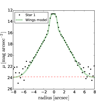
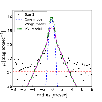
Figure 1: PSF modeling procedure. In top panel, we show the PSF wings modeling by fitting Gaussians and exponential functions to the surface brightness of a saturated star (Star 1). Since this star is saturated, there is no information on the PSF core. In bottom panel, we show the PSF core modeling by fitting a Gaussian function to the surface brightness of a non saturated star (star 2). As can be seen, one part of the wings in this star is under the detection limit (red horizontal segmented line) and another part is noisy, hence the need of the saturated star in order to derive the PSF wings.

3.2.2 Uncertainties

The uncertainties of the real functional form of a given galaxy component leads to the errors in the galaxy models derived using the above-mentioned method. In order to estimate this errors, we follow the procedure described by Olguín-Iglesias et al. (2016); Kotilainen et al. (2016); Olguín-Iglesias et al. (2017) who identify three sources of uncertainties; the PSF model, the sky background and the zeropoint of photometric calibration.

The uncertainties due to the PSF are accounted for by using different PSF models. A number of PSF models can be derived using different stars or different amount of Gaussians and exponentials. The uncertainties due to the sky is derived by running several sky fits in separated regions of 300 pixels $\times$ 300 pixels in the FOV. The zeropoint magnitude depends on the star used to derive it, since they are estimated from the magnitudes of several stars (see Section 3.1) then, we use the zeropoint magnitude variations ($\sim\pm$0.1mag) as another source of uncertainties.

Using these variations, GALFIT is run several times. The resultant fits are used to make a statistic where the best-fit value is the mean and the errors are $\mathrm{\pm 1\sigma}$ for every parameter of the galaxy model.

3.3 Simulations

In order to assure the suitability of the images to resolve galaxy bulges, we performed a set of simulations (Table 5). The simulated galaxies have a nuclear component, represented by a star within the FOV. They also have a Sérsic function, with $n=1$, which represents a bulge and an exponential function representing a disc. The background is taken from the same image as the star of the nuclear component. Every galaxy in the simulation has a different combination of parameters (bulge, disc and nuclear signal to noise ratios; bulge effective radius and seeing). The simulated galaxies are modeled in an identical way to the real galaxies in our sample in order to find whether the quality in our images is good enough to allow an acceptable subtraction of parameters. We found that the ability to properly retrieve the parameters of the bulges, depend both on the size of the bulge, with respect to the seeing, and on the brightness of the bulge with respect to the brightness of the other components. In this way, the parameters of faint bulges (with respect to the nucleus) might be properly retrieve provided that they are large enough (e.g. simulation 42). We note that, although the parameters of a bulge might not be properly retrieved, it might still be detected, although with not enough quality to retrieve its parameters. This means that in some simulations, we were able to properly characterize the nucleus and disc and also detect a residual (unable to be fitted) that we knew, beforehand, it was the bulge (e.g. simulation 1, 6 and 57). We focus on the parameters of bulge and nucleus, although all our simulations include a disc, with the intention of studying the effect of this component on the fittings. Most of the time the disc is not bright enough to hamper the bulge fit. However, the brightness of the bulge and the nucleus can often be high enough to make the modeling and even detection of the disc difficult (e.g. simulations 29, 30 and 75).

In figure 2 we show the set of simulations in a plot of the ratio between the bulge and nucleus S/N versus bulge effective radius normalized to the seeing FWHM. We use signal-to-noise ratios instead of magnitudes because in our simulations we take into account the seeing. The blurring caused by seeing makes the signal of point sources smaller. It also spreads out the light from extended sources, which reduces the measured signal-to-noise and the ability of telescopes to see detail but does not affect the derived magnitudes. Hence, the same source observed with different seeings have the same magnitude, but different signal-to-noise ratios, which is crucial in galaxy fitting. In our simulations, signal-to-noise ratios refer to the peak counts of the source divided by the background noise in the same region. We find the bulk of our sample in the region where the correctly retrieved simulated galaxies lie, which gives us confidence in the reliability of our analysis. We consider a model correct when the difference between a given parameter of the simulation and the same parameter of the model is less than the maximum error for such parameter in our analysis of the real galaxies sample (i.e. magnitude error $\mathrm{Mag_{err}\leq 0.50}$, bulge effective radius error $\mathrm{Re_{err}\leq 100\%}$ and Sérsic index error $\mathrm{n_{err}\leq 1.35}$). Two galaxies in our sample lie outside that region (PMNJ0948+002 and J095820+322401), suggesting that those parameters are incorrectly retrieved, and hence left out of the analysis.

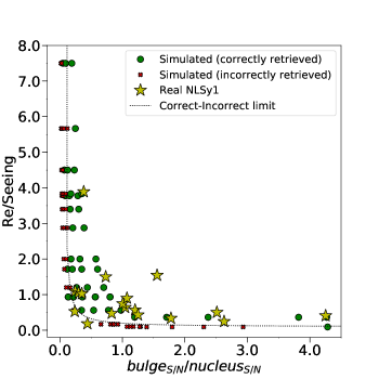
Figure 2: Ratio of the bulge over nucleus S/N versus bulge effective radius normalised to the seeing FWHM. We see the location of the correctly retrieved simulated galaxies (green circles), the incorrectly retrieved simulated galaxies (red crosses) and the real galaxies in our sample (yellow stars, including all 18 galaxies with K–band observations from the NOTcam and fitted in this study, and excluding 4 galaxies from previous studies and/or observed with the ESO/ISAAC, 6 unresolved galaxies and 1 observed only in J–band) A limit that divides the correctly from incorrectly retrieved simulated galaxies is represented by a segmented line.

4 The host galaxies

In table 2, we show a summary of the NLSy1 host and nuclear properties derived from the two-dimensional surface brightness decomposition analysis. In the cases where the host galaxy is not detected we estimated upper limits for their magnitudes by simulating a galaxy (following the method from Kotilainen et al., 2007; Olguín-Iglesias et al., 2016), assuming an average effective radius and Sérsic index from the successfully detected hosts and then, increasing the magnitude until the component becomes detectable with a signal to noise ratio S/N=5, which by our own experience, is required in order to properly retrieve the structural parameters of the galaxy components.

In table 2, we summarize the nuclear and (disky–) bulge properties. However, in Appendix B.1, the detailed fitting results are shown individually for every host in the sample. Out of the sample of 29 radio-loud NLSy1 host galaxies, 21 were successfully detected, 7 of which are $\gamma-$rays emitters and 14 are only radio-loud. For the sample, we estimate an average J–band absolute nuclear and host magnitudes of $\mathrm{M(J){nuclear}=-23.8\pm 1.7}$ and $\mathrm{M(J){bulge}=-23.1\pm 1.0}$ and an average K–band absolute nuclear and host magnitudes of $\mathrm{M(K){nuclear}=-25.6\pm 1.4}$ and $\mathrm{M(K){bulge}=-24.8\pm 1.1}$. The host luminosities for these galaxies are slightly fainter than elliptical galaxies hosting other types of radio–loud AGNs (e.g. Olguín-Iglesias et al., 2016, $\mathrm{M(K)_{FSRQs}=-26.2\pm 0.9}$ and $\mathrm{M(K){BLLacs}=-25.6\pm 0.6}$) and rather similar to those of an $\mathrm{L^{*}}$ galaxy ($\mathrm{M(K)=-24.8\pm 0.3}$ Mobasher et al., 1993).

The average bulge effective radius for J–band and K–band respectively is $\mathrm{R_{eff}=1.9\pm 1.3}$kpc and $\mathrm{R_{eff}=1.5\pm 1.1}$kpc and the average Sérsic index is $\mathrm{n=1.2\pm 0.4}$ for J–band and $\mathrm{n=1.3\pm 0.3}$ for K–band. The Sérsic index can be used as an approximation to classify bulges (either disky, $\mathrm{n<2}$ or classical, $\mathrm{n\geq 2}$, Fisher & Drory, 2008). According to the Sérsic index derived from the photometrical analysis (with the exception of J16410+3454 and J17221+5654, whose Sérsic index might be $\mathrm{n>2}$ given their uncertainties), all the NLSy1s hosts bulges are disc–like. However, it is well known that using the Sérsic index to discern between classical from disc–like bulges can generate many misclassifications (Gadotti, 2009). To address this, we used the fact that disc–like and classical bulges are expected to be structurally different. Therefore, disc–like bulges should not follow the Kormendy relation (inverse relation between $\mathrm{\mu_{e}}$ and $\mathrm{R_{e}}$ found in elliptical galaxies and classical bulges; Kormendy, 1977). In fact, Gadotti (2009) finds that disc–like bulges lie below the Kormendy relation and hence, it can be used to distinguish them from classical bulges.

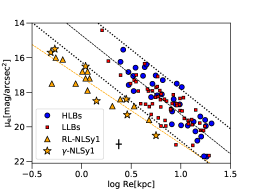
Figure 3: The Kormendy relation in K–band. Symbols are explained in the figure. The bulge effective radius ($\mathrm{logR_{e}}$) is plotted versus the surface brightness at that radius ($\mathrm{\mu_{e}}$). A typical error bar is shown in the lower left corner. Overlayed are a sample of high–luminosity blazars (FSRQs) and low–luminosity blazars (BL Lacs objects) from Olguín-Iglesias et al. (2016), all of them hosted by giant elliptical galaxies. For the blazars sample, we show the 95 per cent prediction bands (dotted lines) and the best linear fit (black dashed line) relation. For the NLSy1s (the 20 detected galaxies in our sample with K–band observations. Missing are 2 with unreliable fittings, 6 undetected galaxies and 1 without K–band observations), we show the best linear fit (yellow dashed line). There are no NLSy1s inside the 95 per cent prediction bands of the Kormendy relation, suggesting that they are hosted by disc–like bulges. A cosmological surface brightness dimming correction of the form $\mathrm{(1+z)^{-4}}$ was applied to all targets (in this work and in Olguín-Iglesias et al. 2016)

In figure 3, we explore the Kormendy relation by plotting the effective radius ($\mathrm{R_{e}}$) versus the surface brightness at the bulge effective radius ($\mathrm{\mu_{e}}$) of the detected hosts with K–band observations . Together, we plot the results of the blazars hosts analysis from Olguín-Iglesias et al. (2016). The blazars hosts show a statistically significant correlation between $\mathrm{R_{e}}$ and $\mathrm{\mu_{e}}$ (the Kormendy relation). On the other hand, the NLSy1s in the sample show a shallower trend. The $\mathrm{95\%}$ prediction bands of the correlation are represented by dotted lines. Since the aim of the prediction bands is to encompass the likely values of future observations from the same sampled population, we might say that it is most likely that the hosts that lie below the lower prediction band are not classical bulges. We can see that all (20 with host detections, K–band observations and inside the ’correctly retrieved’ area) RL–NLSy1s lie below the Kormendy relation and below the 95% prediction bands. If errors are taken into account, 4 NLSy1s might be consistent with classical bulges and 16 are certainly disc–like bulges.

Although these results suggest disc–like systems as RL–NLSy1s hosts, some RL–NLSy1s might be hosted by classical–bulges. Therefore, further studies of their stellar populations and kinematics, using integral field spectroscopy (IFS), will help in understanding their nature. This result is not surprising, since the prevalence of disc–like bulges in this type of AGN hosts have been previously found (e.g. Orban de Xivry et al. 2011; Mathur et al. 2012b). However, very little is known about the presence of radio jets launched from disc galaxies galaxies. In the past, only a small number of disc–like systems were found to be radio galaxies (e.g. Ledlow et al. 1998; Hota et al. 2011; Morganti et al. 2011; Bagchi et al. 2014; Kaviraj et al. 2015; Mao et al. 2015; Singh et al. 2015). However, only three (included in this work) have been found to, additionally, be $\gamma-$rays emitters (León Tavares et al., 2014; Kotilainen et al., 2016; Olguín-Iglesias et al., 2017, 1H0323+342,PKS2004-447, and FBQSJ1644+2619, respectively).

Table 2: Parameters of the host galaxies of the NLSy1 sample derived from GALFIT 2D analysis. All K–corrections were performed using the K-corrections calculator (Chilingarian et al., 2010; Chilingarian & Zolotukhin, 2012)

Name	Band	$M_{nuc}$	$M_{bulge}$	$M_{disc}$	Re (kpc)	$\mu_{e}$	$n$	$r_{s}$	$f_{bar}$	$r_{bar}$(kpc)	$\chi_{best}$	$\chi_{best}/\chi_{psf}$	Int
(1)	(2)	(3)	(4)	(5)	(6)	(7)	(8)	(9)	(10)	(11)	(12)	(13)	(14)
1H0323+342γ	J/K	$-$23.00/$-$24.74	$-$22.53/$-$24.15	$-$23.49/$-$24.93	1.48/1.40	16.89/15.14	0.88/1.24	3.36/3.15	–	–	1.280	–	Y
		(0.01/0.01)	(0.01/0.01)	(0.01/0.01)	(0.01/0.01)	(0.01/0.01)	(0.002)
SBS0846+513γ	J/K	$-$27.14/$-$28.99	$>-23.89/>-25.68$	–	–	–	–	–	–	–	1.646/2.296	1	Y
		(0.36/0.38)									(0.001/0.002)
J093241+53063γ	K	$-26.90$	$-25.25$	–	5.57	20.50	1.21	–	–	–	1.167	0.40	Y
		(0.30)	(0.39)		(0.58)	(0.48)	(0.70)				(0.001)
PMNJ0948+002γ×	J/K	$-27.39/-29.50$	$-24.53/-26.91$	$-25.19/-27.59$	1.82/0.90	19.5/17.5	1.00/1.50	10.04/18.66	–	–	1.718	0.36	N
		(0.40/0.39)	(0.39/0.41)	(0.40/0.41)	(0.33/0.36)	(0.33/0.30)	(0.28/0.28)	(0.36/0.38)			(0.002)
J095820+322401γ×	K	$-24.11$	$-22.91$	$-25.94$	1.47	16.76	0.60	10.04	–	–	1.200	0.35	Y
		(0.30)	(0.36)	(0.48)	(0.41)	(0.50)	(0.89)	(0.36)			(0.001)
FBQS J1102+2239	J/K	$-25.09/-26.78$	$-23.78/-25.41$	$-23.53/-25.74$	4.08/4.78	21.5/19.6	1.00/1.00	11.06/16.24	–	–	1.200	0.32	Y
		(0.28/0.29)	(0.32/0.30)	(0.31/0.34)	(0.42/0.40)	(0.33/0.31)	(0.31/0.31)	(0.41/0.40)			(0.002)
IRAS11598-0112	J/K	$-23.43/-25.69$	$-21.79/-24.66$	$-23.30/-24.98$	0.79/0.87	21.5/16.5	1.12/1.08	2.24/2.47	0.12/0.09	10.46/10.46	1.192/1.467	0.30/0.28	Y
		(0.39/0.37)	(0.38/0.37)	(0.39/0.38)	(0.30/0.31)	(0.32/0.31)	(0.31/0.30)	0.50/0.48			(0.003/0.003)
RXSJ12002-0046	J/K	$-22.51/-24.01$	$-22.79/-24.22$	$-22.99/-24.16$	1.39/1.16	18.5/16.8	1.10/1.08	4.50/4.15	–	–	1.170/191	0.38/0.38	Y
		(0.35/0.37)	(0.38/0.36)	(0.38/0.38)	(0.30/0.31)	(0.30/0.30)	(0.30/0.30)	0.30/0.31			(0.002/0.002)
J12176+6546	J/K	$-24.75/-26.86$	$>-23.56/>-24.65$	–	–	–	–	–	–	–	1.241/1.558	1.00/1.00	N
		(0.37/0.38)									(0.002/0.002)
4C+04.42γ	J	-27.93	$>-25.88$	–	–	–	–	–	–	–	1.200	1.00	N
		(0.37)	–								(0.002)
RXSJ12278+3215	J/K	$-$24.44/-26.24	$>-23.10/>-25.94$	–	–	–	–	–	–	–	2.030	1.00	N
		(0.38/0.38)									(0.001)
SDSS J124634.65+023809γ	K	$-$25.01	$-$24.44	-25.02	2.85	18.4	0.81	6.28	–	–	1.188	0.36	Y
		(0.41)	(0.48)	(0.39)	(0.73)	(0.78)	(0.70)	(0.30)			(0.001)
J13374+6005	J/K	$-22.84/-24.49$	$-21.88/-23.54$	$-22.30/-23.15$	1.11/1.15	19.5/17.9	1.10/1.00	2.42/3.16	0.14/–	11.54/–	1.167/1.205	0.36	N
		(0.37/0.39)	(0.39/0.41)	(0.39/0.40)	(0.28/0.30)	(0.29/0.31)	(0.32/0.35)	(0.30/0.34)			(0.001/0.002)
J14033+0222	J/K	$-21.91/-24.18$	$-22.98/-24.38$	-22.89/-24.60	3.98/3.39	19.7/18.8	1.11/1.05	7.26/6.70	0.27/0.27	13.29/12.51	1.168/1.172	0.37	N
		(0.37/0.38)	(0.39/0.39)	(0.41/0.42)	(0.33/0.35)	(0.30/0.30)	(0.30/0.30)	0.37/0.35			(0.001/0.001)
J142106+385522γ	K	$-26.63$	$-25.68$	$-25.94$	2.89	19.3	1.11	25.08	–	–	1.185	0.31	Y
		(0.35)	(0.37)	(0.41)	(0.46)	(0.42)	(0.38)	(0.57)			(0.001)
J14506+5919	J/K	$-22.45/-24.77$	$-21.90/-24.14$	$-22.80/-25.01$	0.74/0.56	20.5/16.00	1.10/1.15	4.40/4.84	0.22/0.22	7.98/9.14	1.161/1.175	0.34/0.32	Y
		(0.36/0.39)	(0.39/0.40)	(0.39/0.40)	(0.37/0.39)	(0.31/0.30)	(0.30/0.39)	(0.39/0.39)			(0.001/0.001)
B31441+476γ	K	-28.48	$>-27.66$	–	–	–	–	–	–	–	1.276	1.00	N
		(0.40)									(0.002)
PKS1502+036γ∗	J/K	$-24.17/-25.12$	$-23.80/-25.96$	$-24.28/-26.30$	1.05/0.49	15.5/15.7	1.06/1.15	4.11/4.17	–	–	1.577/1.236	0.35/0.34	Y
		(0.38/0.39)	(0.39/0.38)	(0.39/0.41)	(0.64/0.70)	(0.36/0.39)	(0.60/76)	(0.30/0.30)			(0.001/0.001)
SBS 1517+520	J/K	$-24.51/-27.42$	$-24.33/-26.54$	-24.04/-26.32	2.44/2.44	19.1/18.4	1.05/1.10	8.66/5.75	0.09/0.09	10.26/10.26	1.201/1.241	0.35/0.34	Y
		(0.39/0.38)	(0.38/0.39)	(0.37/0.37)	(0.32/0.33)	(0.32/0.32)	(0.32/0.32)	(0.30/0.33)			(0.002/0.002)
B2 1546+35A	J/K	$-24.78/-26.38$	$-24.19/-24.74$	$-23.12/-25.69$	0.96/2.06	16.5/18.8	1.18/0.98	3.99/10.52	–	–	1.161/1.153	0.32	Y
		(0.32/0.30)	(0.29/0.32)	(0.31/0.31)	(0.84/0.33)	(0.90/0.32)	(0.62/0.41)	(0.41/0.41)			(0.001/0.001)
J16290+4007	J/K	$-23.85/-25.86$	$>-22.64/-24.35$	–	–	–	–	–	–	–	1.118	1.00	Y
		(0.37/0.39)									(0.002)
RXSJ16333+4718	J/K	$-22.90/-24.40$	$-22.35/-23.22$	$-23.01/-24.15$	3.61/0.50	22.5/17.5	1.10/1.21	8.50/2.83	0.14/0.12	5.04/5.04	1.299/1.310	0.32	Y
		(0.37/0.37)	(0.39/0.38)	(0.39/0.39)	(0.31/1.58)	(0.32/1.40)	(0.35/0.55)	0.34/0.34			(0.001/0.001)
2E1640+5345	J/K	$-21.69/-23.73$	$-23.40/-24.52$	$-24.21/-25.14$	0.45/0.64	17.5/16.6	1.10/1.09	4.50/5.72	0.07/0.08	7.65/6.17	1.178/1.133	0.35	N
		(0.40/0.39)	(0.37/0.37)	(0.39/0.39)	(0.32/0.32)	(0.40/0.38)	(0.32/0.32)	(0.31/0.31)			(0.001/0.001)
J16410+3454	J/K	$-21.27/-24.35$	$-23.55/-24.65$	$-24.18/-25.55$	0.83/0.98	17.5/16.8	2.24/1.53	4.34/4.01	0.22/0.22	21.20/21.10	1.192/1.169	0.30	Y
		(0.39/0.38)	(0.39/0.39)	(0.38/0.39)	(0.49/0.46)	(0.34/0.38)	(0.43/0.42)	(0.35/0.33)			(0.001/0.001)
FBQSJ1644+2619γ	J/K	$-22.51/-24.80$	$-21.41/-24.21$	$-22.90/-24.85$	0.96/1.10	17.5/16.5	1.80/1.90	6.65/7.68	-/0.17	-/8.13	1.160	0.37	Y
		(0.43/0.24)	(0.40/0.32)	(0.35/0.38)	(0.32/0.34)	(0.30/0.31)	(1.31/1.35)	(0.45/1.14)			(0.027)
B31702+457	K	$-23.88$	$-25.09$	$-23.63$	1.21	17.2	1.03	5.97	–	–	2.021	0.35	N
		(0.28)	(0.32)	(0.30)	(0.36)	(0.43)	(0.41)	(0.29)			(0.003)
J17221+5654	J/K	$-23.84/-25.64$	$-23.95/-24.95$	$-23.12/-24.35$	0.71/1.11	18.3/17.2	2.10/2.12	4.34/4.01	–	–	1.164/1.172	0.27/0.30	Y
		(0.35/0.36)	(0.38/0.39)	(0.39/0.39)	(0.34/0.36)	(0.40/0.35)	(0.33/0.32)	(0.33/0.32)			(0.001/0.001)
PKS2004$-$447γ∗	J/K	$-22.56/-24.79$	$-22.91/-24.50$	$-23.05/-24.40$	0.72/0.53	16.6/15.5	1.15/1.08	3.65/2.51	-/0.13	-/7.59	1.403	0.29	Y
		(0.32/0.25)	(0.29/0.28)	(0.27/0.30)	(0.34/0.42)	(0.20/0.19)	(0.10/0.35)	(0.32/0.32)			(0.025)
IRAS22453$-$1744	J	$-23.34$	$-24.10$	–	2.28	17.5	0.90	–	–	–	1.176	0.27	Y
		(0.35)	(0.36)		(0.29)	(0.35)	(0.30)				(0.001)

Column (1) gives the galaxy name; (2) the observed band; (3), (4) and (5) the nuclear, bulge and disc absolute magnitudes for the best-fit model in the observed band. When the galaxy is not detected, we determine an upper limit by simulating a bulge with average parameters. (6) Bulge effective radius; (7) the bulge model surface brightness at the effective radius; (8) the bulge model Sérsic index; (9) the disc model scale length; (10) bar strength; (11) bar length; (12) the reduced $\chi^{2}$ for the best-fit model; (13) the ratio between best-fit $\chi^{2}$ and the PSF-fit $\chi^{2}$; (14) if the galaxy shows some sign of interaction (Y), otherwise (N).
^∗ Galaxies observed using the ISAAC on the ESO/VLT
^γ $\gamma-$ray emitting NLSy1 galaxies
^× Galaxies with unreliable fittings according to our simulations (see Section 3.3).

The uniqueness of the hosts of NLSy1s (and nearby environment), might hint at how these galaxies acquired such properties. Spiral arms, bar incidence, interactions evidence, etc., could shed some light on the fueling mechanisms needed by the central supermassive black hole to form and develop powerful relativistic jets. Therefore, in the following sections we discuss on the specific features that the hosts of the galaxies in the sample show.

4.1 Bar frequency

Through a simple visual inspection, some galaxies reveal the presence of a bar in their brightness distributions. However, in order to have a quantitative identification of these bars, we adopt an analysis based on the ellipse fit to the galaxy isophotes, where radial variations of ellipticity ($\epsilon$) and position angle (P.A.), exhibit the existence, ellipticity and extent of the bar. Moreover, some bars detected by this way, might not be obvious at a glance. The detection of bars using this method consists on finding a local maximum in $\epsilon$, which indicates the bar end. Along the bar, the P.A. should remain constant, thus along the suspected bar, the P.A. should not change much (typically $\mathrm{\Delta\textrm{PA}\lesssim 20^{\circ}}$, Wozniak et al. 1995; Jogee et al. 1999; Menéndez-Delmestre et al. 2007). At larger radius, further away from the bar end, we should measure the ellipticity and P.A. of the disc then, the ellipticity should drop (at least 0.1; $\mathrm{\Delta\epsilon\geq 0.1}$) and most likely the P.A. will change. In Appendix B.2 we show the plots of P.A. and ellipticity versus radius of 10 of the galaxies that fulfill this criteria (the other two galaxies in the sample with detected bars are shown in Kotilainen et al., 2016; Olguín-Iglesias et al., 2017). Thus, the detected hosts with bars represent 52% (77% RL–NLSy1s and 20% $\gamma-$NLSy1s) of the galaxies in the sample, in comparison, Laurikainen et al. (2004) finds bars in 62%$\pm 9\%$ of Seyfert galaxies. It must be stressed that, although near-IR imaging (specially K–band) provides a reliable assessment of the bar fraction, we might miss some bars given the relative high redshift of some of the galaxies in the sample (e.g. J17221+5654 is the galaxy with the highest redshift $\mathrm{z=0.426}$ and a bar detection).

In addition to finding bars, the radial variations of ellipticity and P.A., help in estimating their ellipticity and length. Ellipticity has been shown to be a good bar strength indicator (Laurikainen et al., 2002). Abraham & Merrifield (2000) defined a bar strength parameter given by

$$\mathrm{f_{bar}=\frac{2}{\pi}\left(arctan\left(1-\epsilon_{bar}\right)^{-1/2}-arctan\left(1-\epsilon_{bar}\right)^{1/2}\right)},$$ (3)

where $\mathrm{\epsilon_{bar}}$ is the bar ellipticity at the bar end. Using this parameter, we find that, for our sample, $\mathrm{f_{bar}=0.13\pm 0.06}$. By comparing this value with the findings of Laurikainen et al. 2007 (average $\mathrm{f_{bar}=0.20\pm 0.03}$, from 216 galaxies observed in the NIR, including all Hubble types), we note that the bar strengths for our NLSy1s sample is rather low. By contrast, we find that the average bar length of our sample ($\mathrm{r_{bar}=9.8kpc\pm 1.8}$) is large when compared either with late type galaxies or early type galaxies ($\mathrm{\sim 0.5-3.5kpc}$ and $\mathrm{\sim 1-10kpc}$, respectively; Erwin, 2005). We note that, even if we assume that the galaxies with no bars detected in our sample have the shortest bars (0.5 kpc), the average bar length would be 5.9 kpc, still larger than the average for late type galaxies (2 kpc), early type galaxies (5.5 kpc) or both early and late type galaxies (3.75 kpc). These results might hint to the necessary conditions to properly channel the fuel towards the center of the galaxy to feed the black hole and trigger its activity. According to bar models by Athanassoula (1992), weak bars promote the inflow of gas toward the inner Lindblad resonance (ILR), and forms a nuclear ring. As long as the bar pattern speed remains low, the ILR is kept, which occurs provided that bars are long. If dynamical instabilities via gradual build-up of material show, material from that nuclear ring would flow inward and trigger the black hole activity, as hypothesize by Laurikainen et al. (2002). Low and steady evolution (secular evolution) might, thus, be capable of producing AGN as powerful as to launch radio jets.

4.2 Mergers and galaxy interactions

Secular evolution driven by stellar asymmetries (i.e. bars, lopsidedness, spiral patterns and other coherent structures) can be strengthened by external processes such as tidal interactions and mergers (Mapelli et al., 2008; Reichard et al., 2009). In our sample, 62% of the galaxies show some sign of merger, interaction or off centered components (9 $\gamma-$NLSy1s and 9 RL–NLSy1s, including both detected and not detected hosts). This result is important since both, observations and simulations suggest that AGN activity is closely related to galaxy interactions and mergers (e.g., Di Matteo et al., 2003; Ellison et al., 2011; Silverman et al., 2011; Koss et al., 2012; Ellison et al., 2013; Capelo et al., 2015).

Particularly, in the case of the $\gamma-$NLSy1s, we note that only 3 out of 12 $\gamma-$NLSy1s do not show signs of interactions (PMNJ0948+0022, $z=0585$; 4C+04.42, $z=0.996$ and B3 1441+476, $z=705$), considering their high redshift and that only one of these hosts is detected. The large fraction of interactions in the $\gamma-$NLSy1s of the sample (75% against 53%, when compared with RL–NLSy1s), largely consist of the host itself and another, significantly smaller, galaxy or faint tidal feature (i.e. minor mergers; however, spectroscopic data is required to confirm the idea of these features as interactions).

This result is important since simulations (e.g. Qu et al., 2011) show that the angular momentum decreases more significantly when the stellar disc undergoes a minor merger than when it evolves in isolation. Hence, the difference in power between RL–NLSy1s and $\gamma-$NLSy1s, might thus be the result of the difference between the processes that drive their evolution. In this way, our findings suggest secular evolution as a process capable of producing, not only radio, but also $\gamma-$ray emitting jets.

Another important finding in our study is that, not only discs might be off-centered with respect to the nucleus, also some bulges might . This behavior has not only been predicted by simulations (Hopkins et al., 2012) but also previously observed. The first offset AGN reported was the Seyfert 1 galaxy NGC 3227 (Mediavilla & Arribas, 1993), where the region of broad emission lines is offset from the kinematic center by $\sim 0.250$ kpc. Another important example is the low–luminosity AGN NGC 3115 (Menezes et al., 2014), with an AGN located at a projected distance of $\sim 0.014$ kpc from the stellar bulge. Similarly, using GALFIT and observations from Chandra/ACIS and the Hubble Space Telescope, Comerford et al. (2015) analyzed a sample of 12 dual AGN candidates at $\mathrm{z<0.34}$ and discovered 6 systems that are either dual or offset AGNs with separations $\mathrm{\Delta x<10}$kpc. Finally, here we find a total of 6 systems (see Table 3) where the stellar bulge is offset from the AGN by projected distances $\mathrm{\Delta x<1.5}$kpc

Table 3: Summary of galaxies with offset AGNs.

Galaxy	Redshift	$\mathrm{\Delta x}$(arcsec)	$\mathrm{\Delta x}$(kpc)
RXSJ12002–0046	0.179	0.24	0.73
J142106+385522 γ	0.490	0.25	1.50
J14506+5919	0.202	0.23	0.76
B2 1546+35A	0.479	0.24	1.42
J17221+5654	0.426	0.23	1.30
IRAS 22453–1744	0.117	0.71	1.50

Column (1) gives the galaxy name; (2) the redshift of the system; (3) and (4) the projected separation between the stellar bulge and the AGN in arcsec and kpc, respectively. The typical error is $\pm 0.16^{\prime\prime}$, derived as described in section 3.2.2.
^γ $\gamma-$ray emitting NLSy1 galaxy

This finding strongly suggests an important connection between AGNs and galaxy mergers. Two likely scenarios where the AGN is off–centered with respect to the stellar bulge are explained on the basis of galaxy mergers. On the one hand, the black hole of the observed AGN and another (inactive) black hole form a binary system. The inactive black hole is located in the center of stellar bulge, and thus the AGN is offset with respect to it (Menezes et al., 2014). On the other hand, two black holes might have already coalesced which caused the formation of gravitational waves, which in turn, asymetrically push the system to shaped it to its current form (Merritt, 2006; Blecha & Loeb, 2008; Sundararajan et al., 2010; Blecha et al., 2019, and references therein). This important finding might help in constraining SMBH-galaxy co-evolution theoretical studies and simulations where most of the times, a stationary central black hole is assume.

4.2.1 Notes on individual galaxies

Here, we provide a short description of the characteristics that each interacting galaxy shows (for images, see Appendix B.1).

• 1H 0323+342. The closest $\gamma-$ray emitter NLSy1 galaxy. In this galaxy a ringed structure is seen which is interpreted as “suggestive evidence for a recent violent dynamical interaction” by León Tavares et al. (2014), where an extensive discussion on this galaxy can be found.

• SBS 0846+513. The host galaxy of this $\gamma-$NLSy1 is not detected, therefore it was modeled using a PSF. A bright and close companion ($\mathrm{<5}$arcsec) is clearly detected. Also, a spiral galaxy in the foreground is observed.

• J093241+53063. A source with a disc–like bulge, with Sérsic index $n=1.21\pm 0.70$. Although no disc is detected, a faint companion is.

• J095820+322401. Although its relative high redshift ($\mathrm{z=0.53}$), we detect a faint close neighbor in this galaxy. When analysed further, an even fainter disc is reveled in our analysis. The disc is off–centered with respect to the nucleus and bulge. This, maybe due to the action exerted by its alleged neighbor.

• FBQSJ1102+2239. This galaxy represents a classical encounter between two disc galaxies. Very similar both in J– and K–bands, a remnant of the disc is detected in the AGN host. The companion keeps an spiral arm and it is barely connected with the main AGN host. Another blob is observed, an HII region, which is part of the system (according to optical spectra).

• IRAS 11598-0112. The AGN host is modeled using a disc–like bulge and a disc. However, two spiral-arm-like features are included in the model. More interestingly, another component (probably a disky bulge) is detected inside the main disc.

• SDSS J124634.65+023808. An AGN dominated galaxy modeled using a bulge and an exponential disc. It shows a close and faint feature which is fitted using an exponential disc.

• J14033+0222. An apparent simple barred galaxy. However, the disc is off-centered with respect to the AGN and bulge (in both, J– and K–bands), which suggests to a not obvious interaction. Since both, bar and disc have exponential profiles and the bar is faint, only one exponential was needed to model both.

• J142106+385522. The host galaxy of this $\gamma-$NLSy1 was modeled using a bulge and a disc. In the image, a faint tail–like feature (which was not modeled due to its intensity) is observed. Suggestion of an interaction are observed in its off–centered disc.

• PKS1502+036. A clear companion only visible in J–band. The companion seems close, however, this galaxy does not show asymmetries as others in the sample. Although D’Ammando et al. (2018) finds it hosted in an elliptical galaxy, we find a better fit using a disc–like host.

• SBS1517+520. In this galaxy, the asymmetry of its surface brightness profile and its off centered disc (more evident in the K–band), hint towards some type of disruption induced by an interaction.

• B2 1546+35A. When the host is decomposed into bulge and disc, the different parts are off centered with respect to each other. While the host galaxy image, both in J– and K–bands, looks similar, when it is represented using its surface brightness profile, the two bands differ.

• RXSJ16333+4718. Two disc galaxies interacting. Seemingly, the companion is also face-on. Again, the host galaxy shows a greater effect of the interaction on one of the bands. While in K–band, the bulge seems a bit off centered, in the J–band, both the disc and the bulge shows greater impact on its morphology.

• J16410+3454. This galaxy shows a feature that emerges after the fitting of a bulge+disc+AGN model. This additional component is modeled using a Sérsic profile with $\mathrm{n\approx 1}$. The main disc seems off centered in the radial profiles (maybe because of the effect of the interaction).

• FBQS J1644+2619. In J–band, a ring feature shows, whose formation process might be that described by Athanassoula et al. (1997) and that PKS 2004-447 might be undergoing. Besides, a faint disruption of the ring suggests an interaction. On the other hand, in K–band, a bar is observed and the ring features is almost absent. An extensive discussion on these features is found on Olguín-Iglesias et al. (2016).

• J17221+5654. The host galaxy was modeled using a bulge and a disc. In both J– and K–bands a small companion is detected a few arcseconds away from the host center. The companion seems to be interacting with the main galaxy since the components of the AGN host are off centered; more evident in K–band.

• PKS 2004-447. This barred galaxy shows two faint spiral arms, one of which is more open. It is a very good example of part of the evolution of the simulations by Athanassoula et al. (1997), where the impact of a small companion on a barred galaxy leads to the formation of a ring. For a detailed discussion on this galaxy see Kotilainen et al. (2016).

• IRAS 22453-1744. A bulge with a Sérsic index $\mathrm{n=0.90\pm 0.30}$ was used to model the host. However, the AGN and host are off-centered. The most likely reason is the close (merged) companion with a complex morphology that is difficult to characterize.

4.3 AGN, bulge and disc (J-K) colours

Subsample	$(J-K)_{Bulge}$	$(J-K)_{Disc}$	$(J-K)_{Nuclear}$
All	$1.7\pm 0.7$	$1.7\pm 0.5$	$2.0\pm 0.5$
RL–NLSy1s	$1.5\pm 0.5$	$1.6\pm 0.6$	$2.0\pm 0.5$
$\gamma-$NLSy1s	$2.1\pm 0.5$	$1.8\pm 0.4$	$1.9\pm 0.5$

Table 4: Average $\mathrm{J-K}$ colours for the bulge, disc and nucleus of the host galaxies in the sample.

Table 4 shows the average J-K colours of the main components of the host galaxies in the sample (whenever they have both, J– and K–band information). We see that the disc and nuclear J-K colours remain virtually unchanged whether the subsample includes $\gamma-$NLSy1s or only RL–NLSy1s. We also note that, unexpectedly, bulge and disc colors for RL–NLSy1s are the same within errors (i.e. bulges are as blue as discs, when disc are expected to be bluer, Moriondo et al., 1998; Seigar & James, 1998). This result is thus consistent with star–forming bulges, which imply large gas reservoirs.

On the other hand, the average J-K bulge colour changes depending on the subsample, being redder for $\gamma-$NLSy1s ($\mathrm{J-K=2.1\pm 0.5}$). According to findings by Glass & Moorwood (1985); Seigar & James (1998), NIR colours $\mathrm{J-K\approx 2.0}$, could be the result of a dust-embedded AGN or a nuclear starbursts (if the component is extended, i.e. in bulges). Bulge reddening might be linked to the large fraction of $\gamma-$NLSy1s showing signs of minor mergers. Thus, according to these results, interactions are likely to play an important role in the nuclear activity of the galaxies in our sample.

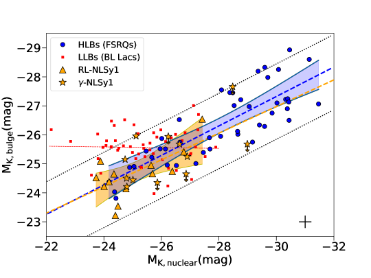
Figure 4: Plot of the nuclear K-band magnitude versus the bulge K-band magnitude for the host galaxies of the sample. Symbols are explained in the figure. Upper limits for unresolved galaxies are shown as down arrows. We show the 25 detected and undetected galaxies in our sample with K–band observations. Missing are 2 with unreliable fittings and 2 without K–band observations. Overlayed is a sample of blazars from Olguín-Iglesias et al. (2016), where the galaxies were analysed in K–band. For the blazars sample we show the best linear fits (dashed blue line for FSRQs and dashed red line for BL Lacs) and the 95 per cent prediction bands (dotted black lines). The 99 per cent confidence intervals are shown for FSRQs (blue shade) and NLSy1s (yellow shade). For the NLSy1s sample we show the best linear fit (green solid line). All K–corrections were performed using the K-corrections calculator (Chilingarian et al., 2010; Chilingarian & Zolotukhin, 2012)

5 AGN-host connection

In figure 4, we explore the $\mathrm{M_{K,nuclear}-M_{K,bulge}}$ plot for our sample. The first thing we notice is that most of the sample data points fall in the bottom left corner, where high luminosity blazars (HLB), i.e. FSRQs and low luminosity blazars (LLB), i.e. BL Lacs coincide. However, three $\gamma-$NLSy1s (only one with host galaxy detection) are brighter and lie $\sim 3$mag apart from the group and two (also $\gamma-$NLSy1s) are fainter and lie $\sim 1$mag appart. At first glance the bulk of RL–NLSy1s, are part of either HLB or LLB. A further analysis shows that, if we include the NLSy1s in the HLB sample, the best linear fit marginally lies inside the 99% confidence intervals of the FSRQs best linear fit. There is a statistically significant positive correlation for the FSRQs sample ($\mathrm{r=0.8}$, $\mathrm{p=4\times 10^{-12}}$) which is kept virtually unchanged ($\mathrm{p\approx 10^{-12}}$) when the RL–NLSy1s are added to the FSRQs.

When we analyze the NLSy1s sample alone, a statistically significant positive correlation is observed ($\mathrm{r=0.6}$, $\mathrm{p=1\times 10^{-3}}$). Whether the NLSy1s sample belongs to the FSRQs sample or not, its positive trend suggests that their jets also stimulate starburst activity in their hosts.

The results presented above suggest either FSRQs and RL–NLSy1s accretion modes locate them close to each other in the $\mathrm{M_{K,nuclear}-M_{K,bulge}}$ plot. Bearing in mind that both, FSRQs and NLSy1s, are thought to acrete matter very efficiently via accretion discs, this is expected.

In order to rule out the scenario where RL–NLSy1s behave as LLB/BL Lacs (since, independently of nuclear magnitude, BL Lacs show a narrow range of bulge magnitudes, where the bulk of RL–NLSy1s bulge magnitudes also reside), we perform a two-dimensional Kolmogorov-Smirnov test for the bulge and nuclear magnitudes of BL Lacs and RL–NLSy1s. According to the results of this test ($\mathrm{p\approx 3.0^{-4}}$) there is a statistically significant difference between the samples, suggesting that, in the $\mathrm{M_{K,nuclear}-M_{K,bulge}}$ plot, BL Lacs and RL–NLSy1s are not similar.

Previous studies, conducted to RL–NLSy1s, had already supported the idea that, when compared with blazars, RL–NLSy1s are particularly similar to FSRQs (e.g. Paliya et al., 2013; Foschini et al., 2015; Paliya & Stalin, 2016). Provided that RL–NLsy1s are hosted by spiral galaxies, what our findings suggest, might be a substantive contribution since blazars are known to be hosted by elliptical galaxies and powered by massive black holes.

The positive trend in the NLSy1s and FSRQs samples clearly suggest a positive feedback scenario. The AGN outflows can induce star formation, both in the galactic disc through compression of molecular clouds Silk (2013) or directly in the outflowing gas Ishibashi & Fabian (2012).

6 Summary

We have presented near–infrared images of a sample of 29 radio–loud NLSy1 host galaxies, 12 of which are also classified as $\gamma-$NLSy1s. By thoroughly analyzing their 2D surface brightness distribution, we successfully detected 21 hosts (14 RL–NLSy1s and 7 $\gamma-$NLSy1s). Our near–infrared study allowed us to compare the photometrical properties of RL–NLSy1s with another type of AGN capable of launching powerful radio jets, namely blazars (both BL Lacs and FSRQs). The main findings of our study are summarized below.

• The photometrical properties derived by our 2D analysis for a sample of RL–NSLy1s suggests that, consistent with radio-quiet NLSy1s and opposite to the jet paradigm, powerful relativistic jets can be launched from disc–like systems instead of elliptical galaxies or classical bulges.

• Secular evolution driven by the peculiar bar properties in our sample (long and weak) might be responsible for channeling fuel towards the center of the galaxy to feed the black hole and trigger the nuclear activity, whereas the nuclear activity in $\gamma-$NLSy1s could be the result of a similar process enhanced by minor mergers.

• RL–NLSy1s bulges and discs show the same average NIRcolour $\mathrm{(J-K)_{Disc}=1.6\pm 0.6}$ and $\mathrm{(J-K)_{bulge}=1.5\pm 0.5}$. Since discs are expected to be bluer, this result is consisting with star–forming bulges, suggesting large gas reservoirs. On the other hand, $\gamma-$NLSy1s bulges show an average NIR colour $\mathrm{(J-K)_{AGN}=2.1\pm 0.5}$. This reddening (with respect to RL–NLSy1s) suggests a nuclear starburts, probably, linked to the large fraction of minor mergers shown by $\gamma-$NLSy1s, which in turn, could make a difference between RL– and $\gamma-$NLSy1s nuclear activity.

• We have discovered 6 systems showing an offset stellar bulge with respect to the AGN (with separations $\mathrm{\Delta<1.5}$kpc). This might be the result of a galaxy merger, strongly suggesting an important connection between AGNs and galaxy mergers.

• Hints of positive feedback are suggested when we plot $\mathrm{M_{K,nuclear}}$ versus $\mathrm{M_{K,bulge}}$ of the sample. We find that RL–NLSy1s behave in a similar manner as FSRQs (or high luminosity blazars), which might be the result of a similar accretion mode between RL–NLSy1s and FSRQs.

Appendix A Simulations

	Simulation parameters					Retrieved parameters
	Seeing	$\mathrm{m_{nuclear}}$	$\mathrm{m_{bulge}}$	$\mathrm{Re}$	$\mathrm{m_{disc}}$		$\mathrm{m_{nuclear}}$	$\mathrm{m_{bulge}}$	$\mathrm{R_{e}}$	n	$\mathrm{m_{disc}}$	$\mathrm{R_{s}}$	Model quality
	(arcsec)			(arcsec)					(arcsec)			(arcsec)
1	0.60	16.00	18.50	0.10	15.00		15.90	20.75	2.13	0.06	15.09	2.83	bad
2	0.60	15.00	17.00	0.10	15.00		14.85	19.63	2.09	0.19	15.09	2.87	bad
3	0.60	14.00	15.50	0.10	15.00		13.79	17.71	0.40	0.06	15.09	2.79	bad
4	0.60	13.00	14.00	0.10	15.00		12.66	17.92	0.21	1.84	15.09	2.75	bad
5	0.60	12.00	12.50	0.10	15.00		11.64	13.54	0.25	0.05	15.09	2.81	bad
6	0.60	16.00	18.50	0.10	15.00		15.90	20.75	2.13	0.06	15.09	2.83	bad
7	0.60	15.00	17.00	0.10	15.00		14.85	19.63	2.09	0.19	15.09	2.87	bad
8	0.60	14.00	15.50	0.10	15.00		13.79	17.71	0.40	0.06	15.09	2.79	bad
9	0.60	13.00	14.00	0.10	15.00		12.66	17.92	0.21	1.84	15.09	2.75	bad
10	0.60	12.00	12.50	0.10	15.00		11.64	13.54	0.25	0.05	15.09	2.81	bad
11	0.60	16.00	18.50	0.56	18.50		15.99	18.84	0.56	0.54	15.09	2.79	good
12	0.60	15.00	17.00	0.56	15.00		15.00	17.09	0.56	0.88	15.09	2.78	good
13	0.60	14.00	15.50	0.56	15.00		14.00	15.52	0.56	0.97	15.09	2.78	good
14	0.60	13.00	14.00	0.56	15.00		13.00	14.01	0.56	0.99	15.09	2.78	good
15	0.60	12.00	12.50	0.56	15.00		12.00	12.50	0.56	1.00	15.09	2.78	good
16	0.60	16.00	18.50	0.56	18.50		15.99	18.84	0.56	0.54	15.09	2.79	good
17	0.60	15.00	17.00	0.56	15.00		15.00	17.09	0.56	0.88	15.09	2.78	good
18	0.60	14.00	15.50	0.56	15.00		14.00	15.52	0.56	0.97	15.09	2.78	good
19	0.60	13.00	14.00	0.56	15.00		13.00	14.01	0.56	0.99	15.09	2.78	good
20	0.60	12.00	12.50	0.56	15.00		12.00	12.50	0.56	1.00	15.09	2.78	good
21	0.60	16.00	18.50	1.20	15.00		15.99	18.16	**	2.13	15.09	2.61	bad
22	0.60	15.00	17.00	1.20	15.00		14.95	16.29	**	**	15.06	2.11	bad
23	0.60	14.00	15.50	1.20	15.00		14.00	15.50	1.20	0.98	15.07	2.74	good
24	0.60	13.00	14.00	1.20	15.00		13.00	14.02	1.20	0.99	15.06	2.71	good
25	0.60	12.00	12.50	1.20	15.00		12.00	12.51	1.20	1.00	15.05	2.69	good
26	0.60	16.00	18.50	2.30	15.00		16.00	**	**	0.08	15.06	2.71	bad
27	0.60	15.00	17.00	2.30	15.00		15.00	15.43	3.42	0.99	15.92	3.87	bad
28	0.60	14.00	15.50	2.30	15.00		14.00	15.01	3.03	1.12	16.30	5.15	bad
29	0.60	13.00	14.00	2.30	15.00		13.00	13.68	2.65	1.16	**	**	good
30	0.60	12.00	12.50	2.30	15.00		12.00	12.41	2.39	1.06	**	**	good
31	0.60	16.00	18.50	3.40	15.00		15.99	**	**	**	15.10	2.58	bad
32	0.60	15.00	17.00	3.40	15.00		14.98	**	**	**	15.10	2.13	bad
33	0.60	14.00	15.50	3.40	15.00		14.00	15.26	4.95	0.67	15.38	0.69	bad
34	0.60	13.00	14.00	3.40	15.00		13.00	15.26	4.96	0.67	13.97	0.65	bad
35	0.60	12.00	12.50	3.40	15.00		12.00	12.42	2.07	1.19	**	**	good
36	0.60	16.00	18.50	4.50	15.00		16.00	**	**	**	15.03	2.81	bad
37	0.60	15.00	17.00	4.50	15.00		15.00	**	**	**	14.91	2.79	bad
38	0.60	14.00	15.50	4.50	15.00		14.00	15.12	3.91	0.86	15.43	3.54	good
39	0.60	13.00	14.00	4.50	15.00		13.00	13.94	4.13	0.93	15.25	3.92	good
40	0.60	12.00	12.50	4.50	15.00		12.00	12.59	4.62	0.99	14.45	2.34	good
41	0.70	16.00	18.50	1.20	15.00		15.99	19.21	0.00	15.28	15.09	2.62	bad
42	0.70	15.00	17.00	1.20	15.00		15.00	17.50	1.32	1.02	15.09	2.80	good
43	0.70	14.00	15.50	1.20	15.00		14.02	15.04	2.42	2.37	16.33	3.82	good
44	0.70	13.00	14.00	1.20	15.00		13.00	14.02	1.21	0.99	15.07	2.70	good
45	0.70	12.00	12.50	1.20	15.00		12.00	12.51	1.21	1.00	15.06	2.68	good
46	0.80	16.00	18.50	2.30	15.00		16.00	16.43	70.00	0.04	15.10	2.62	bad
47	0.80	15.00	17.00	2.30	15.00		14.99	16.51	2.72	0.92	15.25	2.95	bad

Table 5: Parameters of the sample of simulated galaxies (columns 2-6) and the retrieved parameters of the simulated galaxies when they are modeled in an identical way to the real galaxies in our sample (columns 7-12).

Column (1) gives the simulation number; (2) the simulation seeing; (3) and (4) the simulated nuclear and bulge magnitudes; (5) the simulated bulge effective radius; (6) the simulated disc magnitude; (7) the modeled nuclear magnitude; (8) the modeled bulge magnitude; (9) the modeled bulge effective radius; (10) the modeled bulge Sérsic index (11) the modeled disc magnitude; (12) the modeled disc scale length; (13) the quality with which the simulation was modeled.
The ’**’ symbol shows a physically improbable parameter.
All the simulated galaxies have bulges with Sérsic indexes (n=1) and discs with scale lengths ($\mathrm{R_{s}=3.0}$ arcsec).

	Simulation parameters					Retrieved parameters
	Seeing	$\mathrm{m_{nuclear}}$	$\mathrm{m_{bulge}}$	$\mathrm{Re}$	$\mathrm{m_{disc}}$		$\mathrm{m_{nuclear}}$	$\mathrm{m_{bulge}}$	$\mathrm{R_{e}}$	n	$\mathrm{m_{disc}}$	$\mathrm{R_{s}}$	Model quality
	(arcsec)			(arcsec)					(arcsec)			(arcsec)
48	0.80	14.00	15.50	2.30	15.00		14.00	15.02	3.02	1.11	16.31	4.94	bad
49	0.80	13.00	14.00	2.30	15.00		13.00	13.68	2.65	1.16	26.10	0.01	good
50	0.80	12.00	12.50	2.30	15.00		12.00	12.41	2.39	1.06	**	**	good
51	0.90	16.00	18.50	3.40	15.00		16.02	25.61	**	6.35	15.10	2.55	bad
52	0.90	15.00	17.00	3.40	15.00		15.00	16.69	**	**	14.96	2.58	bad
53	0.90	14.00	15.50	3.40	15.00		14.00	15.68	5.29	1.20	14.95	2.22	good
54	0.90	13.00	14.00	3.40	15.00		13.00	13.78	3.46	0.97	15.99	4.15	good
55	0.90	12.00	12.50	3.40	15.00		12.00	12.41	3.47	1.01	17.07	**	good
56	1.00	16.00	18.50	0.10	15.00		15.89	17.28	3.30	0.70	15.24	3.02	bad
57	1.00	15.00	17.00	0.10	15.00		14.99	17.00	1.14	**	15.09	2.87	bad
58	1.00	14.00	15.50	0.10	15.00		13.77	18.46	**	**	15.09	2.78	bad
59	1.00	13.00	14.00	0.10	15.00		12.72	15.22	**	**	15.12	2.94	bad
60	1.00	12.00	12.50	0.10	15.00		11.60	13.64	**	**	15.10	2.82	bad
61	1.00	16.00	18.50	0.56	18.50		16.03	17.52	1.77	**	15.11	2.85	bad
62	1.00	15.00	17.00	0.56	15.00		15.00	17.02	0.54	1.09	15.09	2.79	good
63	1.00	14.00	15.50	0.56	15.00		14.00	15.51	0.55	1.00	15.09	2.78	good
64	1.00	13.00	14.00	0.56	15.00		13.00	14.00	0.56	1.00	15.09	2.78	good
65	1.00	12.00	12.50	0.56	15.00		12.00	12.50	0.56	1.00	15.09	2.78	good
66	1.00	16.00	18.50	1.20	15.00		16.21	16.87	**	**	15.08	2.63	bad
67	1.00	15.00	17.00	1.20	15.00		14.98	16.24	**	0.99	15.06	2.25	bad
68	1.00	14.00	15.50	1.20	15.00		14.00	15.57	1.20	0.94	15.07	2.72	good
69	1.00	13.00	14.00	1.20	15.00		13.00	14.03	1.20	0.98	15.05	2.69	good
70	1.00	12.00	12.50	1.20	15.00		12.00	12.51	1.20	0.99	15.04	2.66	good
71	1.00	16.00	18.50	3.40	15.00		16.00	**	**	**	15.07	2.63	bad
72	1.00	15.00	17.00	3.40	15.00		14.99	15.99	3.52	0.80	15.43	3.17	bad
73	1.00	14.00	15.50	3.40	15.00		14.00	17.12	**	0.12	14.62	2.29	bad
74	1.00	13.00	14.00	3.40	15.00		13.01	13.67	3.54	1.03	15.32	**	good
75	1.00	12.00	12.50	3.40	15.00		12.00	12.41	3.47	1.01	16.25	**	good
76	1.00	16.00	18.50	4.50	15.00		16.00	28.53	**	0.41	15.04	2.69	bad
77	1.00	15.00	17.00	4.50	15.00		15.00	19.53	**	1.16	14.92	2.79	bad
78	1.00	14.00	15.50	4.50	15.00		14.00	15.87	3.63	0.78	14.90	3.06	good
79	1.00	13.00	14.00	4.50	15.00		13.00	14.20	4.84	0.98	14.69	2.43	good
80	1.00	12.00	12.50	4.50	15.00		12.00	12.41	4.50	0.99	**	**	good
81	1.10	14.00	13.20	0.10	15.00		13.74	13.35	0.11	0.64	15.09	2.79	good
82	1.10	14.00	14.00	0.10	15.00		13.55	14.62	**	**	15.11	2.94	bad
83	1.10	14.00	15.00	0.10	15.00		13.68	16.95	0.12	**	15.11	2.88	bad
84	1.10	14.00	15.50	0.10	15.00		13.79	17.57	0.50	**	15.09	2.78	bad
85	1.10	14.00	14.50	0.10	15.00		13.59	15.91	0.13	4.11	15.10	2.79	bad
86	1.10	14.00	13.20	0.40	15.00		13.95	13.23	0.40	0.95	15.09	2.75	good
87	1.10	14.00	14.00	0.40	15.00		13.95	14.05	0.40	0.91	15.09	2.76	good
88	1.10	14.00	15.00	0.40	15.00		13.96	15.11	0.40	0.81	15.09	2.76	good
89	1.10	14.00	13.00	0.40	15.00		13.94	13.02	0.40	0.96	15.09	2.75	good
90	1.10	14.00	14.50	0.40	15.00		13.96	14.58	0.40	0.87	15.09	2.76	good

Table B1: Continued…

Column (1) gives the simulation number; (2) the simulation seeing; (3) and (4) the simulated nuclear and bulge magnitudes; (5) the simulated bulge effective radius; (6) the simulated disc magnitude; (7) the modeled nuclear magnitude; (8) the modeled bulge magnitude; (9) the modeled bulge effective radius; (10) the modeled bulge Sérsic index (11) the modeled disc magnitude; (12) the modeled disc scale length; (13) the quality with which the simulation was modeled.
The ’**’ symbol shows a physically improbable parameter.
All the simulated galaxies have bulges with Sérsic indexes (n=1) and discs with scale lengths ($\mathrm{R_{s}=3.0}$ arcsec).

Appendix B Morphological analysis

B.1 Models

Figure 5: Surface brightness profile decomposition of the host galaxies in the sample. Top left: Shows the observed image. Top middle: Shows the image of the model used to describe the surface brightness distribution. Top right: Shows the residual image. Middle: Radial profile of the surface brightness distribution. The symbols and the main parameters of the models are explained in the plots. For the complete Appendix see the online material. Bottom: Residuals.

Figure 6:

IRAS 11598-0112 (J–band)	IRAS 11598-0112 (K–band)

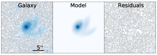
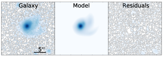
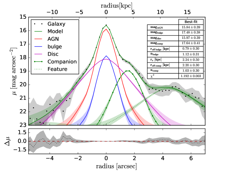
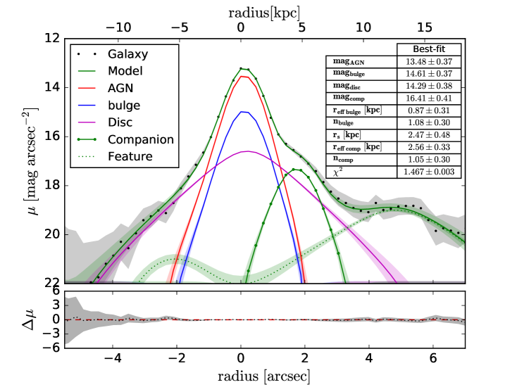
B.2 Bar test

Figure 7: Radial variation of ellipticity $\epsilon$ (blue circles) and of position angle PA (red squares) derived by ellipse fitting to the galaxy isophotes. Only the host galaxies that fulfill the criteria to identify bars are shown (see Section 4.1). For the complete Appendix see the online material.

IRAS 11598$-$0112 (J–band)

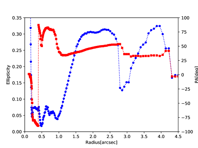
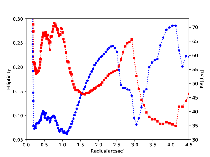
IRAS 11598$-$0112 (K–band)

References

- Abdo et al. (2009a) Abdo A. A., et al., 2009a, ApJ, 699, 976
- Abdo et al. (2009b) Abdo A. A., et al., 2009b, ApJ, 707, L142
- Abraham & Merrifield (2000) Abraham R. G., Merrifield M. R., 2000, AJ, 120, 2835
- Athanassoula (1992) Athanassoula E., 1992, MNRAS, 259, 345
- Athanassoula et al. (1997) Athanassoula E., Puerari I., Bosma A., 1997, MNRAS, 286, 284
- Bagchi et al. (2014) Bagchi J., et al., 2014, ApJ, 788, 174
- Bertin & Arnouts (1996) Bertin E., Arnouts S., 1996, A&ASS, 117, 393
- Blecha & Loeb (2008) Blecha L., Loeb A., 2008, MNRAS, 390, 1311
- Blecha et al. (2019) Blecha L., Brisken W., Burke-Spolaor S., Civano F., Comerford J., Darling J., Lazio T. J. W., Maccarone T. J., 2019, Astro2020: Decadal Survey on Astronomy and Astrophysics, 2020, 318
- Capelo et al. (2015) Capelo P. R., Volonteri M., Dotti M., Bellovary J. M., Mayer L., Governato F., 2015, MNRAS, 447, 2123
- Chilingarian & Zolotukhin (2012) Chilingarian I. V., Zolotukhin I. Y., 2012, MNRAS, 419, 1727
- Chilingarian et al. (2010) Chilingarian I. V., Melchior A.-L., Zolotukhin I. Y., 2010, MNRAS, 405, 1409
- Comerford et al. (2015) Comerford J. M., Pooley D., Barrows R. S., Greene J. E., Zakamska N. L., Madejski G. M., Cooper M. C., 2015, ApJ, 806, 219
- D’Ammando et al. (2012) D’Ammando F., et al., 2012, MNRAS, 426, 317
- D’Ammando et al. (2015) D’Ammando F., Orienti M., Larsson J., Giroletti M., 2015, MNRAS, 452, 520
- D’Ammando et al. (2018) D’Ammando F., Acosta-Pulido J. A., Capetti A., Baldi R. D., Orienti M., Raiteri C. M., Ramos Almeida C., 2018, MNRAS, 478, L66
- Di Matteo et al. (2003) Di Matteo T., Croft R. A. C., Springel V., Hernquist L., 2003, ApJ, 593, 56
- Ellison et al. (2011) Ellison S. L., Patton D. R., Mendel J. T., Scudder J. M., 2011, MNRAS, 418, 2043
- Ellison et al. (2013) Ellison S. L., Mendel J. T., Patton D. R., Scudder J. M., 2013, MNRAS, 435, 3627
- Erwin (2005) Erwin P., 2005, MNRAS, 364, 283
- Fabian (2012) Fabian A. C., 2012, ARA&A, 50, 455
- Ferrarese & Merritt (2000) Ferrarese L., Merritt D., 2000, ApJL, 539, L9
- Fisher & Drory (2008) Fisher D. B., Drory N., 2008, in Funes J. G., Corsini E. M., eds, Astronomical Society of the Pacific Conference Series Vol. 396, Formation and Evolution of Galaxy Disks. p. 309
- Foschini (2011) Foschini L., 2011, in Narrow-Line Seyfert 1 Galaxies and their Place in the Universe. p. 24 (arXiv:1105.0772)
- Foschini et al. (2015) Foschini L., et al., 2015, A&A, 575, A13
- Gadotti (2009) Gadotti D. A., 2009, mnras, 393, 1531
- Gebhardt et al. (2000) Gebhardt K., et al., 2000, ApJL, 539, L13
- Glass & Moorwood (1985) Glass I. S., Moorwood A. F. M., 1985, MNRAS, 214, 429
- Gültekin et al. (2009) Gültekin K., et al., 2009, ApJ, 698, 198
- Heckman & Best (2014) Heckman T. M., Best P. N., 2014, ARA&A, 52, 589
- Hopkins et al. (2012) Hopkins P. F., Hernquist L., Hayward C. C., Narayanan D., 2012, MNRAS, 425, 1121
- Hota et al. (2011) Hota A., et al., 2011, MNRAS, 417, L36
- Hyvönen et al. (2007) Hyvönen T., Kotilainen J. K., Falomo R., Örndahl E., Pursimo T., 2007, A&A, 476, 723
- Ishibashi & Fabian (2012) Ishibashi W., Fabian A. C., 2012, MNRAS, 427, 2998
- Jogee et al. (1999) Jogee S., Kenney J. D. P., Smith B. J., 1999, ApJ, 526, 665
- Kaspi et al. (2000) Kaspi S., Smith P. S., Netzer H., Maoz D., Jannuzi B. T., Giveon U., 2000, ApJ, 533, 631
- Kaviraj et al. (2015) Kaviraj S., Shabala S. S., Deller A. T., Middelberg E., 2015, MNRAS, 454, 1595
- Komossa et al. (2006) Komossa S., Voges W., Xu D., Mathur S., Adorf H.-M., Lemson G., Duschl W. J., Grupe D., 2006, AJ, 132, 531
- Kormendy (1977) Kormendy J., 1977, ApJ, 218, 333
- Koss et al. (2012) Koss M., Mushotzky R., Treister E., Veilleux S., Vasudevan R., Trippe M., 2012, ApJ, 746, L22
- Kotilainen et al. (1998a) Kotilainen J. K., Falomo R., Scarpa R., 1998a, A&A, 332, 503
- Kotilainen et al. (1998b) Kotilainen J. K., Falomo R., Scarpa R., 1998b, A&A, 336, 479
- Kotilainen et al. (2005) Kotilainen J. K., Hyvönen T., Falomo R., 2005, A&A, 440, 831
- Kotilainen et al. (2007) Kotilainen J. K., Falomo R., Labita M., Treves A., Uslenghi M., 2007, ApJ, 660, 1039
- Kotilainen et al. (2016) Kotilainen J. K., Tavares J. L., Olguin-Iglesias A., Baes M., Anorve C., Chavushyan V., Carrasco L., 2016, preprint, (arXiv:1609.02417)
- Laurikainen et al. (2002) Laurikainen E., Salo H., Rautiainen P., 2002, MNRAS, 331, 880
- Laurikainen et al. (2004) Laurikainen E., Salo H., Buta R., 2004, ApJ, 607, 103
- Laurikainen et al. (2007) Laurikainen E., Salo H., Buta R., Knapen J. H., 2007, MNRAS, 381, 401
- Ledlow et al. (1998) Ledlow M. J., Owen F. N., Keel W. C., 1998, ApJ, 495, 227
- León Tavares et al. (2014) León Tavares J., et al., 2014, ApJ, 795, 58
- Liao et al. (2015) Liao N.-H., Liang Y.-F., Weng S.-S., Berton M., Gu M.-F., Fan Y.-Z., 2015, preprint, (arXiv:1510.05584)
- Magorrian et al. (1998) Magorrian J., et al., 1998, AJ, 115, 2285
- Mao et al. (2015) Mao M. Y., et al., 2015, MNRAS, 446, 4176
- Mapelli et al. (2008) Mapelli M., Moore B., Bland-Hawthorn J., 2008, MNRAS, 388, 697
- Mathur et al. (2012a) Mathur S., Fields D., Peterson B. M., Grupe D., 2012a, ApJ, 754, 146
- Mathur et al. (2012b) Mathur S., Fields D., Peterson B. M., Grupe D., 2012b, ApJ, 754, 146
- Mediavilla & Arribas (1993) Mediavilla E., Arribas S., 1993, Nature, 365, 420
- Menéndez-Delmestre et al. (2007) Menéndez-Delmestre K., Sheth K., Schinnerer E., Jarrett T. H., Scoville N. Z., 2007, ApJ, 657, 790
- Menezes et al. (2014) Menezes R. B., Steiner J. E., Ricci T. V., 2014, ApJ, 796, L13
- Merritt (2006) Merritt D., 2006, ApJ, 648, 976
- Mobasher et al. (1993) Mobasher B., Sharples R. M., Ellis R. S., 1993, MNRAS, 263, 560
- Moorwood et al. (1998) Moorwood A., et al., 1998, The Messenger, 94, 7
- Morganti et al. (2011) Morganti R., Holt J., Tadhunter C., Ramos Almeida C., Dicken D., Inskip K., Oosterloo T., Tzioumis T., 2011, A&A, 535, A97
- Moriondo et al. (1998) Moriondo G., Giovanardi C., Hunt L. K., 1998, A&AS, 130, 81
- Olguín-Iglesias et al. (2016) Olguín-Iglesias A., et al., 2016, MNRAS, 460, 3202
- Olguín-Iglesias et al. (2017) Olguín-Iglesias A., Kotilainen J. K., León Tavares J., Chavushyan V., Añorve C., 2017, MNRAS, 467, 3712
- Orban de Xivry et al. (2011) Orban de Xivry G., Davies R., Schartmann M., Komossa S., Marconi A., Hicks E., Engel H., Tacconi L., 2011, MNRAS, 417, 2721
- Osterbrock & Pogge (1985) Osterbrock D. E., Pogge R. W., 1985, ApJ, 297, 166
- Paliya & Stalin (2016) Paliya V. S., Stalin C. S., 2016, ApJ, 820, 52
- Paliya et al. (2013) Paliya V. S., Stalin C. S., Kumar B., Kumar B., Bhatt V. K., Pandey S. B., Yadav R. K. S., 2013, MNRAS, 428, 2450
- Paliya et al. (2018) Paliya V. S., Ajello M., Rakshit S., Mandal A. K., Stalin C. S., Kaur A., Hartmann D., 2018, ApJ, 853, L2
- Peng et al. (2011) Peng C. Y., Ho L. C., Impey C. D., Rix H.-W., 2011, GALFIT: Detailed Structural Decomposition of Galaxy Images, Astrophysics Source Code Library (ascl:1104.010)
- Qu et al. (2011) Qu Y., Di Matteo P., Lehnert M. D., van Driel W., Jog C. J., 2011, A&A, 535, A5
- Reichard et al. (2009) Reichard T. A., Heckman T. M., Rudnick G., Brinchmann J., Kauffmann G., Wild V., 2009, ApJ, 691, 1005
- Scarpa et al. (2000) Scarpa R., Urry C. M., Falomo R., Pesce J. E., Treves A., 2000, ApJ, 532, 740
- Seigar & James (1998) Seigar M. S., James P. A., 1998, MNRAS, 299, 672
- Silk (2013) Silk J., 2013, ApJ, 772, 112
- Silverman et al. (2011) Silverman J. D., et al., 2011, ApJ, 743, 2
- Singh et al. (2015) Singh V., Ishwara-Chandra C. H., Sievers J., Wadadekar Y., Hilton M., Beelen A., 2015, MNRAS, 454, 1556
- Skrutskie et al. (2006) Skrutskie M. F., et al., 2006, AJ, 131, 1163
- Stickel et al. (1991) Stickel M., Padovani P., Urry C. M., Fried J. W., Kuehr H., 1991, apj, 374, 431
- Sundararajan et al. (2010) Sundararajan P. A., Khanna G., Hughes S. A., 2010, Phys. Rev. D, 81, 104009
- Tremaine et al. (2002) Tremaine S., et al., 2002, ApJ, 574, 740
- Urry et al. (2000) Urry C. M., Scarpa R., O’Dowd M., Falomo R., Pesce J. E., Treves A., 2000, ApJ, 532, 816
- Wozniak et al. (1995) Wozniak H., Friedli D., Martinet L., Martin P., Bratschi P., 1995, A&AS, 111, 115
- Yao et al. (2015) Yao S., Yuan W., Zhou H., Komossa S., Zhang J., Qiao E., Liu B., 2015, MNRAS, 454, L16