Inelastic collisions in radiofrequency-dressed mixtures of ultracold atoms

Abstract

Radiofrequency ()-dressed potentials are a promising technique for manipulating atomic mixtures, but so far little work has been undertaken to understand the collisions of atoms held within these traps. In this work, we dress a mixture of $\mathrm{{}^{85}Rb}$ and $\mathrm{{}^{87}Rb}$ with radiation, characterize the inelastic loss that occurs, and demonstrate species-selective manipulations. Our measurements show the loss is caused by two-body $\mathrm{{}^{87}Rb}$+$\mathrm{{}^{85}Rb}$ collisions, and we show the inelastic rate coefficient varies with detuning from the resonance. We explain our observations using quantum scattering calculations, which give reasonable agreement with the measurements. The calculations consider magnetic fields both perpendicular to the plane of RF polarization and tilted with respect to it. Our findings have important consequences for future experiments that dress mixtures with fields.

Experiments that use mixtures of ultracold atoms are now established as versatile quantum simulators for a range of physical phenomena. For systems of many particles, recent studies have examined superfluidity Ferrier-Barbut et al. (2014), non-equilibrium dynamics in many-body quantum systems Cetina et al. (2016), and the interactions mediated by a bath DeSalvo et al. (2019). At the single-particle level, experiments have observed diffusion Hohmann et al. (2017), chemical reactions Liu et al. (2018) and ultralow-energy collisions Schmidt et al. (2019). Mixtures of ultracold atoms are also used as a starting point for the production of ultracold molecules Papp and Wieman (2006); De Marco et al. (2019). These experiments have been made possible by techniques to manipulate ultracold mixtures and their constituents, and new investigations will become possible as laboratory methods evolve.

A number of different techniques are used to trap and manipulate cold atoms. In this paper we consider -dressed potentials, which confine cold atoms through a combination of static and radiofrequency magnetic fields Garraway and Perrin (2016); Perrin and Garraway (2017). Notable advantages of this technique include smooth, defect-free traps and low heating rates Merloti et al. (2013). The potential can be shaped by controlling the -dressing field Hofferberth et al. (2006), or by adding additional components Harte et al. (2018). Furthermore, the potential may be combined with additional time-averaging fields to produce trap geometries such as rings or double wells Lesanovsky and von Klitzing (2007); Gildemeister et al. (2010); Sherlock et al. (2011). The confining forces depend only on an atom’s magnetic structure, unlike optical methods which depend on electronic structure. Therefore, -dressed potentials permit species-selective manipulations of mixtures that have similar confinement in dipole traps, such as mixtures of hyperfine states or isotopes Extavour et al. (2006); Navez et al. (2016); Bentine et al. (2017).

In spite of the advantages of -dressed potentials, there has so far been little consideration of the collisional stability of mixtures that are trapped using them. In this work, we investigate collisions in an -dressed mixture of $\mathrm{{}^{85}Rb}$ and $\mathrm{{}^{87}Rb}$ atoms in their lower hyperfine states. We observe a rapid loss of $\mathrm{{}^{85}Rb}$ atoms from the trap due to two-body $\mathrm{{}^{87}Rb}$+$\mathrm{{}^{85}Rb}$ inelastic collisions, which occur through a spin-exchange mechanism. We use a theoretical model to explain the inelastic collisions, and compare predictions from quantum scattering calculations to our measurements of the two-body rate coefficients. Our results suggest that spin-exchange collisions will occur for most combinations of alkali-metal atoms in -dressed potentials. Furthermore, our results verify our understanding of ultracold collisions in the presence of strong, resonant dressing fields.

This paper is structured as follows. In sec:APRevieweq:Eq. (I)sec:APReviewfig:Fig. Isec:APReviewtab:Table Isec:APReviewappendix:Appendix Isec:APReviewsec:Section I we explain the dressed-atom picture. In sec:ExperimentalSequenceeq:Eq. (II)sec:ExperimentalSequencefig:Fig. IIsec:ExperimentalSequencetab:Table IIsec:ExperimentalSequenceappendix:Appendix IIsec:ExperimentalSequencesec:Section II we describe the experimental procedure used to produce cold clouds of $\mathrm{{}^{85}Rb}$ and $\mathrm{{}^{87}Rb}$, and we demonstrate species-selective manipulations. In sec:Resultseq:Eq. (III)sec:Resultsfig:Fig. IIIsec:Resultstab:Table IIIsec:Resultsappendix:Appendix IIIsec:Resultssec:Section III we present measurements of the inelastic loss, which we show is dominated by two-body $\mathrm{{}^{87}Rb}$+$\mathrm{{}^{85}Rb}$ collisions, and we measure the two-body rate coefficient $k_{2}^{\mathrm{85,87}}$ as a function of magnetic field and field amplitude. In sec:QuantumScatteringCalculationseq:Eq. (IV)sec:QuantumScatteringCalculationsfig:Fig. IVsec:QuantumScatteringCalculationstab:Table IVsec:QuantumScatteringCalculationsappendix:Appendix IVsec:QuantumScatteringCalculationssec:Section IV we discuss the quantum scattering calculations and compare the predicted rate coefficients to the experimental measurements. In sec:semiclassicaleq:Eq. (V)sec:semiclassicalfig:Fig. Vsec:semiclassicaltab:Table Vsec:semiclassicalappendix:Appendix Vsec:semiclassicalsec:Section V we compare our results to a semi-classical model. In sec:Conclusioneq:Eq. (VI)sec:Conclusionfig:Fig. VIsec:Conclusiontab:Table VIsec:Conclusionappendix:Appendix VIsec:Conclusionsec:Section VI we conclude with a discussion of inelastic loss expected for other species.

I The -dressed atom

In this work, we consider rubidium atoms in their ground electronic state. We adopt the common collision convention that lower-case quantum numbers refer to individual atoms and upper-case quantum numbers refer to a colliding pair. An atom is described by its electron spin $s=1/2$ and nuclear spin $i$, which couple to form a resultant spin $f$. In a static magnetic field $B_{\mathrm{0}}$* along the $z$ axis, the Hamiltonian for each atom is

$$\mathcal{H}_{\text{atom}}=\zeta\hat{i}\cdot\hat{s}+\left(g_{S}\hat{s}_{z}+g_{i}\hat{i}_{z}\right)\mu_{\mathrm{B}}{}B_{\mathrm{0}}{},$$ (1)

where $\zeta$ is the hyperfine coupling constant, $\mu_{\mathrm{B}}$ is the Bohr magneton and $g_{S}$ and $g_{i}$ are electron and nuclear spin $g$-factors with the sign convention of Arimondo et al. Arimondo et al. (1977). At the low magnetic fields considered here, each atomic state splits into substates with a well-defined projection $m_{f}$ of the total angular momentum $f$ along $B_{\mathrm{0}}$*. In this regime, $f$ is nearly conserved but the individual projections $m_{s}$ and $m_{i}$ of $s$ and $i$ are not. At low fields, the field-dependent terms in eq:moneq:Eq. (1)eq:monfig:Fig. 1eq:montab:Table 1eq:monappendix:Appendix 1eq:monsec:Section 1 may be approximated in the coupled basis $\ket{f,m_{f}}$ to

$$\mathcal{H}_{\text{atom}}=g_{f}\mu_{\mathrm{B}}{}B_{\mathrm{0}}{}m_{f},$$ (2)

where substates $m_{f}$ are separated in energy by the Zeeman splitting and $g_{f}$ is the Landé $g$-factor.

In addition to the static magnetic field, we consider a radiofrequency field with angular frequency $\omega$ that is $\sigma_{-}$ polarized about the $z$ axis, with $\vec{B}_{\textrm{\rf{}}}(t)=B_{\mathrm{\rf{}}}{}[\vec{e}_{x}\cos\omega{}t-\vec{e}_{y}\sin\omega{}t]$. The Hamiltonian of the field is

$$\mathcal{H}_{\text{rf}}=\hbar\omega{}(N+N_{0}),$$ (3)

where $\hat{N}=\hat{a}_{-}^{\dagger}\hat{a}_{-}-\langle\hat{a}_{-}^{\dagger}\hat{a}_{-}\rangle$ is the photon number with respect to the average photon number $N_{0}=\langle\hat{a}_{-}^{\dagger}\hat{a}_{-}\rangle$, and $\hat{a}_{-}^{\dagger}$ and $\hat{a}_{-}$ are photon creation and annihilation operators for $\sigma_{-}$ photons. For $\sigma_{-}$ polarization, the $N$ photons have angular momentum projection $M_{N}=-N$ onto the $z$ axis.

The Hamiltonian for the interaction of the field with an atom is

$$\mathcal{H}_{\text{int}}=\frac{\mu_{\rm B}B_{\rm rf}}{2\sqrt{N_{0}}}\left[(g_{S}\hat{s}_{+}+g_{i}\hat{i}_{+})\hat{a}_{-}^{\dagger}+(g_{S}\hat{s}_{-}+g_{i}\hat{i}_{-})\hat{a}_{-}\right],$$ (4)

where $\hat{s}_{+}$ and $\hat{s}_{-}$ are raising and lowering operators for the electron spin and $\hat{i}_{+}$ and $\hat{i}_{-}$ are the corresponding operators for the nuclear spin.

The atom-photon interaction for $\sigma_{-}$ polarization conserves $m_{\text{tot}}{}=m_{f}+M_{N}=m_{f}-N$. If the couplings are neglected, states with the same $m_{\text{tot}}{}$ cross as a function of magnetic field at the radiofrequency resonance $\hbar\omega=g_{f}\mu_{\mathrm{B}}{}B_{\mathrm{0}}{}$, as shown by the dashed lines in fig:dressedAtoms_Eseq:Eq. (1)fig:dressedAtoms_Esfig:Fig. 1fig:dressedAtoms_Estab:Table 1fig:dressedAtoms_Esappendix:Appendix 1fig:dressedAtoms_Essec:Section 1. For the frequency of $3.6\text{\,}\mathrm{MHz}$ used in this work, the states $(f,m_{f},N)=(1,+1,1)$, $(1,0,0)$ and $(1,-1,-1)$ of $\mathrm{{}^{87}Rb}$ all cross near $B=$5.12\text{\,}\mathrm{G}$$, and the states $(f,m_{f},N)=(2,+2,2),(2,+1,1)$, $(2,0,0)$, $(2,-1,-1)$ and $(2,-2,-2)$ of $\mathrm{{}^{85}Rb}$ all cross near $B=$7.70\text{\,}\mathrm{G}$$. These crossings become avoided crossings when the couplings of eq:rf_inteq:Eq. (4)eq:rf_intfig:Fig. 4eq:rf_inttab:Table 4eq:rf_intappendix:Appendix 4eq:rf_intsec:Section 4 are included. The eigenstates within each manifold of constant $m_{\text{tot}}$ are labelled by the quantum number $\widetilde{m}$, which takes values in the range $-f$ to $f$. The corresponding eigenenergies are

$$E(\widetilde{m}{},m_{\text{tot}}{})=\hbar\widetilde{m}{}\sqrt{\Omega^{2}+\delta^{2}}-m_{\text{tot}}{}\hbar\omega,$$ (5)

where $\delta=(g_{f}\mu_{\mathrm{B}}{}B_{\mathrm{0}}{}/\hbar-\omega{})$ is the angular frequency detuning from resonance and $\Omega$ is the Rabi frequency on resonance. In an inhomogeneous field, atoms in states for which $\widetilde{m}>0$ may be trapped in the resulting potential minimum Garraway and Perrin (2016); Perrin and Garraway (2017).

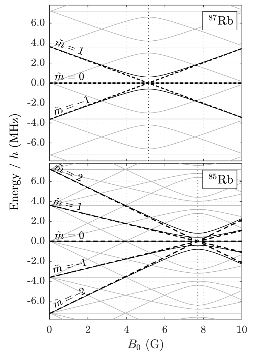
Figure 1: The -dressed eigenstates (solid lines) for $\mathrm{{}^{87}Rb}$ (top) and $\mathrm{{}^{85}Rb}$ (bottom) as a function of magnetic field $B_{\mathrm{0}}$, for $B_{\mathrm{\rf{}}}{}=$0.86\text{\,}\mathrm{G}$$ and $\omega{}=$3.6\text{\,}\mathrm{MHz}$$. A single manifold with $m_{\text{tot}}{}=0$ is emphasized in bold. Dashed lines show the dressed states of this manifold in the limit of zero atom-photon interaction.

II Experimental Methods

In this section, we describe the methods used to cool and trap mixtures of $\mathrm{{}^{85}Rb}$ and $\mathrm{{}^{87}Rb}$. Our apparatus was described previously Harte et al. (2018), and has since been modified to allow the trapping of two species.

An experimental sequence begins by collecting atoms of $\mathrm{{}^{85}Rb}$ and $\mathrm{{}^{87}Rb}$ into a dual-isotope magneto-optical trap (MOT). The cooling and repumping light for $\mathrm{{}^{87}Rb}$ is generated by two external-cavity diode lasers. Each laser is locked to one of the transitions, and injection-locks a laser diode that is current-modulated at a frequency of $1.1\text{\,}\mathrm{GHz}$ (cooling) or $2.5\text{\,}\mathrm{GHz}$ (repumper). The modulation generates sidebands at the frequencies required to laser cool and repump $\mathrm{{}^{85}Rb}$ atoms. Light from the two injection-locked diodes is combined and passed through a tapered amplifier, before illuminating a 3D pyramid MOT, which collects $4\text{\times}{10}^{9}$ atoms of $\mathrm{{}^{87}Rb}$ and $1\text{\times}{10}^{8}$ atoms of $\mathrm{{}^{85}Rb}$. These atoms are optically pumped into their lower hyperfine levels, with $f{}=1$ and $2$ respectively, and the low-field-seeking states are loaded into a magnetic quadrupole trap.

The trapped mixture of isotopes is transported to an ultra-high-vacuum region where it is evaporatively cooled using a weak field, first within a quadrupole trap and then in a Time-Orbiting Potential (TOP) trap, to a temperature of $\sim$0.5\text{\,}\mathrm{\SIUnitSymbolMicro K}$$. This process predominantly ejects $\mathrm{{}^{87}Rb}$ atoms from the trap and the $\mathrm{{}^{85}Rb}$ atoms are sympathetically cooled with minimal loss Bloch et al. (2001). The final atom numbers of each species are controlled by adjusting the power of the cooling light that is resonant with each isotope during the MOT loading stage, which determines the number of atoms initially collected. We observe no evidence of interspecies inelastic loss in these magnetic traps, imposing a bound of $k_{2}^{\mathrm{85,87}}\ll${10}^{-14}\text{\,}{\mathrm{cm}}^{3}\text{\,}{\mathrm{s}}^{-1}$$ on the two-body rate coefficient; this is expected because spin exchange is forbidden between the $(f{},m_{f})=(2,-2)$ and $(1,-1)$ states of $\mathrm{{}^{85}Rb}$ and $\mathrm{{}^{87}Rb}$ respectively.

II.1 Species-selective manipulations

After evaporation, the atoms are loaded into a time-averaged adiabatic potential (TAAP) Lesanovsky and von Klitzing (2007); Gildemeister et al. (2010). This potential is formed by combining a spherical quadrupole field $\vec{B}_{\text{quad}}$, a slow time-averaging field $B_{\mathrm{TA}}$*, and an -dressing field $B_{\mathrm{\rf{}}}*{}$ that is $\sigma_{-}$ polarized in a plane perpendicular to $z$:

$$\vec{B}_{\text{quad}} = B^{\prime}(x\vec{e}_{x}+y\vec{e}_{y}-2z\vec{e}_{z}),$$ (6)

$$B_{\mathrm{\rf{}}}*{} = B_{\text{rf}}\left[\cos{(\omega t)}\vec{e}_{x}-\sin({\omega t})\vec{e}_{y}\right],$$ (7)

$$B_{\mathrm{TA}}*{} = B_{\mathrm{TA}}{}\left[\cos(\omega_{\mathrm{TA}}t)\vec{e}_{x}-\sin(\omega_{\mathrm{TA}}t)\vec{e}_{y}\right].$$ (8)

The field, with $\omega=$3.6\text{\,}\mathrm{MHz}$$, drives transitions between the Zeeman substates so that the atoms are in -dressed eigenstates. The field is resonant with the atomic Zeeman splitting at points on the surface of a spheroid, centered on the quadrupole node, with semi-axes of length $\hbar\omega/g_{f}\mu_{\mathrm{B}}{}B^{\prime}\times\{1,1,0.5\}$ along the $\{\vec{e}_{x},\vec{e}_{y},\vec{e}_{z}\}$ axes. The time-averaging field sweeps this resonant surface in a circular orbit of radius $r_{\mathrm{orbit}}=B_{\mathrm{TA}}{}/B^{\prime}{}$ around the $z$ axis. The frequency of the time-averaging field, $\omega_{\mathrm{TA}}=$7\text{\,}\mathrm{kHz}$$, is slow compared to the Larmor, and Rabi frequencies, so atoms adiabatically follow the -dressed eigenstates as the potential is swept.

For a single species, the TAAP operates in two modes, depending on the value of $B_{\mathrm{TA}}$. When $B_{\mathrm{TA}}{}>\hbar{}\omega/g_{f}\mu_{\mathrm{B}}{}{}$, the resonant spheroid orbits far from the atoms, which are confined near the origin by the rotating field $B_{\mathrm{TA}}$*, as in a TOP trap. When $B_{\mathrm{TA}}{}<\hbar{}\omega{}/g_{f}\mu_{\mathrm{B}}{}$, the resonant spheroid intersects the $z$ axis, forming a double-well potential with minima at positions Lesanovsky and von Klitzing (2007)

$$x=0,y=0,z=\pm\frac{\hbar\omega}{2g_{f}\mu_{\mathrm{B}}{}B^{\prime}{}}\sqrt{1-\left(\frac{g_{f}\mu_{\mathrm{B}}{}B_{\mathrm{TA}}{}}{\hbar\omega}\right)^{2}}.$$ (9)

In this work we load atoms only into the lower well, and henceforth neglect the upper well. The vertical position of the lower well is controlled by changing $B_{\mathrm{TA}}$, which determines the radius of orbit and thus the point of intersection of the resonant spheroid and the $z$ axis.

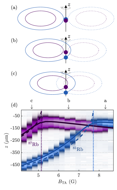
Figure 2: (a-c) The different operating regimes of the dual-species TAAP. Filled circles show the locations of potential minima for $\mathrm{{}^{85}Rb}$ (blue) and $\mathrm{{}^{87}Rb}$ (purple). The ellipses show the resonant spheroids at phases $\omega_{\mathrm{TA}}t=0$ (solid lines) and $\pi$ (dotted lines) of the rotating field $B_{\mathrm{TA}}$*. Three distinct regimes are shown: (a) $\hbar\omega<g_{f}^{85}\mu_{\mathrm{B}}{}B_{\mathrm{TA}}{}$, (b) $g_{f}^{85}\mu_{\mathrm{B}}{}B_{\mathrm{TA}}{}<\hbar\omega<g_{f}^{87}\mu_{\mathrm{B}}{}B_{\mathrm{TA}}{}$, (c) $g_{f}^{87}\mu_{\mathrm{B}}{}B_{\mathrm{TA}}{}<\hbar\omega$. (d) Measurements of the vertical position of $\mathrm{{}^{85}Rb}$ and $\mathrm{{}^{87}Rb}$ clouds as a function of $B_{\mathrm{TA}}$. The observed density distribution for each species along the vertical direction is shown as a vertical slice for each unique value of $B_{\mathrm{TA}}$. The dotted vertical lines show the two resonances, where $g_{f}^{i}\mu_{\mathrm{B}}{}B_{\mathrm{TA}}{}=\hbar\omega$. For each species, the colored lines show the value of $z$ from Eq. (9) (dashed), and the numerically calculated TAAP trap minimum (solid).

The TAAP differs for species with $g$-factors of different magnitude, such as $\mathrm{{}^{85}Rb}$ and $\mathrm{{}^{87}Rb}$ in their lower hyperfine states, which have $g_{f}^{85}\!=\!-1/3$ and $g_{f}^{87}\!=\!-1/2$. fig:SSTAAP_Positionseq:Eq. (2)fig:SSTAAP_Positionsfig:Fig. 2fig:SSTAAP_Positionstab:Table 2fig:SSTAAP_Positionsappendix:Appendix 2fig:SSTAAP_Positionssec:Section 2 shows how the positions of each species change as a function of the time-averaging field $B_{\mathrm{TA}}$. With $B_{\mathrm{TA}}{}>\hbar\omega/g_{f}^{85}\mu_{\mathrm{B}}{}$, the resonant spheroids for both species orbit far from the atoms, which are confined near the origin. This scheme is illustrated in fig:SSTAAP_Positionseq:Eq. (2)fig:SSTAAP_Positionsfig:Fig. 2fig:SSTAAP_Positionstab:Table 2fig:SSTAAP_Positionsappendix:Appendix 2fig:SSTAAP_Positionssec:Section 2a. For $g_{f}^{85}\mu_{\mathrm{B}}{}B_{\mathrm{TA}}{}<\hbar\omega<g_{f}^{87}\mu_{\mathrm{B}}{}B_{\mathrm{TA}}{}$, only the resonant spheroid for $\mathrm{{}^{85}Rb}$ intersects the rotation axis, confining $\mathrm{{}^{85}Rb}$ in the lower well of the TAAP but keeping $\mathrm{{}^{87}Rb}$ confined near the origin by the TOP-like trap, as in fig:SSTAAP_Positionseq:Eq. (2)fig:SSTAAP_Positionsfig:Fig. 2fig:SSTAAP_Positionstab:Table 2fig:SSTAAP_Positionsappendix:Appendix 2fig:SSTAAP_Positionssec:Section 2b. In this configuration, the vertical position of the $\mathrm{{}^{85}Rb}$ potential minimum is strongly affected by $B_{\mathrm{TA}}$, while that of $\mathrm{{}^{87}Rb}$ is not. When $B_{\mathrm{TA}}{}<\hbar\omega/g_{f}^{87}\mu_{\mathrm{B}}{}$, the resonant spheroids for both species intersect the rotation axis, and both are loaded into the lower well of their respective TAAPs, as in fig:SSTAAP_Positionseq:Eq. (2)fig:SSTAAP_Positionsfig:Fig. 2fig:SSTAAP_Positionstab:Table 2fig:SSTAAP_Positionsappendix:Appendix 2fig:SSTAAP_Positionssec:Section 2c.

II.2 Measuring inelastic loss

To observe inelastic loss between $\mathrm{{}^{85}Rb}$ and $\mathrm{{}^{87}Rb}$, we work in the regime in which the clouds of the two species are spatially overlapped, which requires that $g_{f}^{85}\mu_{\mathrm{B}}{}B_{\mathrm{TA}}>\hbar\omega$, as shown in fig:SSTAAP_Positionseq:Eq. (2)fig:SSTAAP_Positionsfig:Fig. 2fig:SSTAAP_Positionstab:Table 2fig:SSTAAP_Positionsappendix:Appendix 2fig:SSTAAP_Positionssec:Section 2. The two isotopes are held in contact for a specified duration, then the remaining atom numbers $\mathcal{N}_{i}$ of both are measured using absorption imaging. The raw images are processed using the fringe-removal algorithm developed by Ockeloen et al. Ockeloen et al. (2010). The temperatures $T_{\mathrm{\mathit{i}}}$ of both species are measured using time-of-flight expansion.

The mixtures used in this work have atom numbers $\mathcal{N}_{85}$, $\mathcal{N}_{87}$ of the two species, with $\mathcal{N}_{85}\ll\mathcal{N}_{87}$; the decrease in $\mathcal{N}_{85}$ over time provides a clear signal to measure the inelastic loss rate. The fractional decrease in $\mathcal{N}_{87}$ is negligible and cannot be distinguished above shot-to-shot variations. The inelastic collisions have a negligible effect on the temperature of $\mathrm{{}^{87}Rb}$, and the $\mathrm{{}^{87}Rb}$ atoms thus provide a large bath of nearly constant density $n_{87}$.

Our -dressed trap confines two states of $\mathrm{{}^{85}Rb}$, with $\widetilde{m}\!=\!1,2$. The two separate clouds that correspond to these states are discernible in absorption images, but their overlap means that only the total atom number $\mathcal{N}_{85}(t)=\mathcal{N}_{1}+\mathcal{N}_{2}$ can be measured accurately. For our experiments, initially $\mathcal{N}_{2}\gg\mathcal{N}_{1}$ because the method used to load the -dressed trap favours projection from $m_{f}=-2$ into $\widetilde{m}{}=2$.

III Inelastic Loss

Including up to 3-body collision processes, $\mathcal{N}_{85}(t)$ decreases at a rate given by

$$\frac{d\mathcal{N}_{85}(t)}{dt}= -\frac{\mathcal{N}_{85}(t)}{\tau_{85}}$$

$$-\int n_{85}(t)\left(k_{2}^{\mathrm{85,87}}n_{87}(t)+k_{3}^{\mathrm{85,87,87}}n_{87}(t)^{2}\right)dV$$

$$-\int n_{85}^{2}(t)\left(k_{2}^{\mathrm{85,85}}+k_{3}^{\mathrm{85,85,87}}n_{87}(t)\right)dV$$

$$-\int n_{85}^{3}(t)\left(k_{3}^{\mathrm{85,85,85}}\right)dV,$$ (10)

where $n_{i}(t)$ are atom number densities, and $\tau_{85}$ is the lifetime of trapped $\mathrm{{}^{85}Rb}$ atoms from one-body losses and collisions with the background gas. The coefficients $k_{j}$ are $j$-body rate coefficients, with the colliding species indicated by the superscript.

For pure $\mathrm{{}^{85}Rb}$ samples, eq:85Losseq:Eq. (III)eq:85Lossfig:Fig. IIIeq:85Losstab:Table IIIeq:85Lossappendix:Appendix IIIeq:85Losssec:Section III reduces to

$$\frac{d\mathcal{N}_{85}(t)}{dt}=-\frac{\mathcal{N}_{85}}{\tau_{85}}-\int k_{2}^{\mathrm{85,85}}n_{85}^{2}dV-\int k_{3}^{\mathrm{85,85,85}}n_{85}^{3}dV.$$ (11)

When only $\mathrm{{}^{85}Rb}$ is present, we observe an exponential decay of $\mathcal{N}_{85}(t)$ with lifetime $\tau_{85}=$43\text{\,}\mathrm{s}$$, and the trapped atoms heating at a rate of $74\text{\,}\mathrm{nK}\text{\,}{\mathrm{s}}^{-1}$ from an initial temperature of $1\text{\,}\mathrm{\SIUnitSymbolMicro K}$. The fitted rate coefficients $k_{2}^{\mathrm{85,85}}$ and $k_{3}^{\mathrm{85,85,85}}$ are consistent with zero, with upper bounds of $k_{2}^{\mathrm{85,85}}<$3\text{\times}{10}^{-12}\text{\,}{\mathrm{cm}}^{3}\text{\,}{\mathrm{s}}^{-1}$$ and $k_{3}^{\mathrm{85,85,85}}<${10}^{-22}\text{\,}{\mathrm{cm}}^{6}\text{\,}{\mathrm{s}}^{-1}$$ in the -dressed trap. These bounds are sufficiently low that the intraspecies inelastic loss is negligible for all experiments discussed in this work.

When both species are present, inelastic collisions cause a rapid loss of $\mathrm{{}^{85}Rb}$, with almost all atoms lost after a few hundred milliseconds. We argue that the loss occurs through two-body $\mathrm{{}^{87}Rb}$+$\mathrm{{}^{85}Rb}$ collisions, as follows. Neglecting both the intraspecies loss and one-body loss, eq:85Losseq:Eq. (III)eq:85Lossfig:Fig. IIIeq:85Losstab:Table IIIeq:85Lossappendix:Appendix IIIeq:85Losssec:Section III approximates to

$$\frac{d\mathcal{N}_{85}(t)}{dt}\approx -\int n_{85}(t)\left(k_{2}^{\mathrm{85,87}}n_{87}+k_{3}^{\mathrm{85,87,87}}n_{87}^{2}\right)dV$$

$$-\int k_{3}^{\mathrm{85,85,87}}n_{85}^{2}(t)n_{87}dV.$$ (12)

Thus, depending on which term dominates, $d\mathcal{N}_{85}/dt$ is proportional to either $n_{85}$ or $n_{85}^{2}$. For an atomic cloud at constant temperature, $n_{i}\propto\mathcal{N}_{i}$.

In fig:85Decay_FitModeleq:Eq. (3)fig:85Decay_FitModelfig:Fig. 3fig:85Decay_FitModeltab:Table 3fig:85Decay_FitModelappendix:Appendix 3fig:85Decay_FitModelsec:Section 3a, we show measurements of $\mathcal{N}_{85}$ against hold time. The total $\mathrm{{}^{85}Rb}$ atom number is well described by a model where the two trapped states of $\mathrm{{}^{85}Rb}$ each decay exponentially, $\mathcal{N}_{85}=\mathcal{N}_{1}+\mathcal{N}_{2}$ with $\mathcal{N}_{i}=A_{i}e^{-\beta_{i}t}$. The different decay constants $\beta_{i}$ arise from the differing overlap of each state’s density distribution with that of $\mathrm{{}^{87}Rb}$. For the measurements in fig:85Decay_FitModeleq:Eq. (3)fig:85Decay_FitModelfig:Fig. 3fig:85Decay_FitModeltab:Table 3fig:85Decay_FitModelappendix:Appendix 3fig:85Decay_FitModelsec:Section 3 the overlap of $\mathrm{{}^{85}Rb}$ atoms in the $\widetilde{m}{}\!=\!2$ state with $\mathrm{{}^{87}Rb}$ is optimized, thus $\beta_{2}\gg\beta_{1}$. A model in which $d\mathcal{N}_{i}(t)/dt\propto\mathcal{N}_{i}^{2}$ shows poor agreement with the data, as shown in fig:85Decay_FitModeleq:Eq. (3)fig:85Decay_FitModelfig:Fig. 3fig:85Decay_FitModeltab:Table 3fig:85Decay_FitModelappendix:Appendix 3fig:85Decay_FitModelsec:Section 3a. From $d\mathcal{N}_{i}/dt\propto\mathcal{N}_{i}$, it follows that one $\mathrm{{}^{85}Rb}$ atom is involved in each inelastic collision.

For short hold times, $t\ll 1/\beta_{1}$, the atom number decays exponentially as

$$\mathcal{N}_{85}(t)\approx A_{2}e^{-\beta_{2}t}+A_{1}.$$ (13)

fig:85Decay_FitModeleq:Eq. (3)fig:85Decay_FitModelfig:Fig. 3fig:85Decay_FitModeltab:Table 3fig:85Decay_FitModelappendix:Appendix 3fig:85Decay_FitModelsec:Section 3b shows $\mathcal{N}_{85}$ as a function of time during the initial fast exponential decay, for different densities of $\mathrm{{}^{87}Rb}$. We fit eq:N85ExpDecayeq:Eq. (13)eq:N85ExpDecayfig:Fig. 13eq:N85ExpDecaytab:Table 13eq:N85ExpDecayappendix:Appendix 13eq:N85ExpDecaysec:Section 13 to the data in fig:85Decay_FitModeleq:Eq. (3)fig:85Decay_FitModelfig:Fig. 3fig:85Decay_FitModeltab:Table 3fig:85Decay_FitModelappendix:Appendix 3fig:85Decay_FitModelsec:Section 3b, and in the inset plot $\beta_{2}$ against $n_{87}^{\text{max}}$, the maximum atom number density of $\mathrm{{}^{87}Rb}$, which occurs at the centre of the trap. The measured decay rate is proportional to $n_{87}^{\text{max}}$, indicating that the inelastic collisions involve a single $\mathrm{{}^{87}Rb}$ atom. Thus we deduce that the inelastic loss arises from a mechanism involving two-body $\mathrm{{}^{87}Rb}$+$\mathrm{{}^{85}Rb}$ collisions.

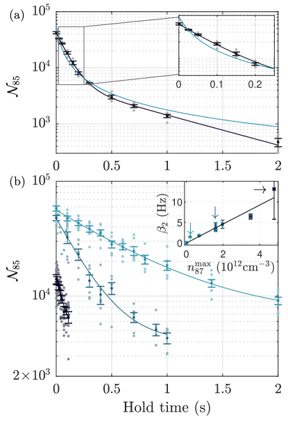
Figure 3: (a) The measured total $\mathrm{{}^{85}Rb}$ atom number $\mathcal{N}_{85}$ as a function of hold time in the trap. The solid black line shows the best fit of a model in which the population of both trapped states of $\mathrm{{}^{85}Rb}$ decays exponentially. The solid blue line shows an alternative model in which each population decays with a rate proportional to $\mathcal{N}_{i}^{2}$. (b) At short hold times the change in atom number is dominated by the exponential atom loss from the state with $\widetilde{m}\!=\!2$. The decay rates in the presence of three different atom number densities of $\mathrm{{}^{87}Rb}$ are shown. Inset: The fitted rate coefficients $\beta_{2}$ are linearly proportional to the peak $\mathrm{{}^{87}Rb}$ atom number density, $n_{87}^{\text{max}}$. Arrows indicate the three sets that are plotted in the outer panel.

Measuring the two-body rate coefficient

Having determined that two-body $\mathrm{{}^{87}Rb}$+$\mathrm{{}^{85}Rb}$ inelastic collisions are the dominant loss mechanism for $\mathrm{{}^{85}Rb}$ in the trapped mixture, we now measure the two-body rate coefficient. eq:85LossWith87eq:Eq. (III)eq:85LossWith87fig:Fig. IIIeq:85LossWith87tab:Table IIIeq:85LossWith87appendix:Appendix IIIeq:85LossWith87sec:Section III further approximates to

$$\frac{d\mathcal{N}_{85}}{dt}\approx-\int k_{2}^{\mathrm{85,87}}n_{85}n_{87}dV$$ (14)

We measure the inelastic loss rate by fitting eq:N85ExpDecayeq:Eq. (13)eq:N85ExpDecayfig:Fig. 13eq:N85ExpDecaytab:Table 13eq:N85ExpDecayappendix:Appendix 13eq:N85ExpDecaysec:Section 13 to $\mathcal{N}_{85}(t)$. As only the total inelastic loss rate is measurable, and $k_{2}^{\mathrm{85,87}}$ varies with position in the trap, we are able to extract only a mean value of $k_{2}^{\mathrm{85,87}}$ that is weighted by the overlap between the species,

$$\langle k_{2}^{\mathrm{85,87}}\rangle=\frac{\int k_{2}^{\mathrm{85,87}}n_{85}n_{87}dV}{\int n_{85}n_{87}dV},$$ (15)

where the term $\int n_{85}n_{87}dV$ is the overlap integral that quantifies the spatial overlap. Hence,

$$\frac{d\mathcal{N}_{85}}{dt}\approx-\langle k_{2}^{\mathrm{85,87}}\rangle\int n_{85}n_{87}dV.$$ (16)

Determining the overlap integral requires knowledge of the atom number densities $n_{i}$. We calculate these densities using measured values of the cloud temperatures, quadrupole field gradient, rotating bias field amplitude, and field. The temperatures are determined from time-of-flight expansion of the clouds, and we find that $T_{\mathrm{87}}$ is independent of hold time. However, it is not possible to determine $T_{\mathrm{85}}$ at arbitrary hold times; the significant $\mathrm{{}^{85}Rb}$ atom loss results in weak absorption imaging signals, which cannot be reliably fitted with Gaussian profiles. Instead, we determine $T_{\mathrm{85}}$ at $t=0$ and assume it is constant thereafter. A Monte-Carlo method is used to determine the uncertainties in $\int n_{85}n_{87}dV$, which incorporate the individual uncertainties (including systematic errors) of all independent parameters. The uncertainties in $\int n_{85}n_{87}dV$ are combined in quadrature with those of the fitted decay rates to determine the uncertainty of $\langle k_{2}^{\mathrm{85,87}}\rangle$.

We explore the dependence of $\langle k_{2}^{\mathrm{85,87}}\rangle$ on the static magnetic field by adjusting $B_{\mathrm{TA}}$, which is akin to a bias field in our setup. This is possible provided the two species remain overlapped, which requires that $B_{\mathrm{TA}}{}>\hbar\omega/(g_{f}^{85}\mu_{\mathrm{B}}{})$, as described in sec:SSTAAPeq:Eq. (II.1)sec:SSTAAPfig:Fig. II.1sec:SSTAAPtab:Table II.1sec:SSTAAPappendix:Appendix II.1sec:SSTAAPsec:Section II.1. For any given value of $B_{\mathrm{TA}}$, collisions occur over a range of different static magnetic fields because of the field gradient that is required to confine the atoms. As such, we compare our measured rate coefficients as a function of the overlap-weighted average $\langle B_{\mathrm{0}}\rangle$, defined analogously to $\langle k_{2}^{\mathrm{85,87}}\rangle$. Our measurements are shown in fig:k2vBeq:Eq. (4)fig:k2vBfig:Fig. 4fig:k2vBtab:Table 4fig:k2vBappendix:Appendix 4fig:k2vBsec:Section 4, for three different amplitudes of the -dressing field. We observe that the two-body rate coefficient increases with decreasing $\langle B_{\mathrm{0}}\rangle$, and within the uncertainties observe no clear dependence on amplitude. We also plot the values of $\langle k_{2}^{\mathrm{85,87}}\rangle$ predicted from our scattering calculations, which are described in the next section.

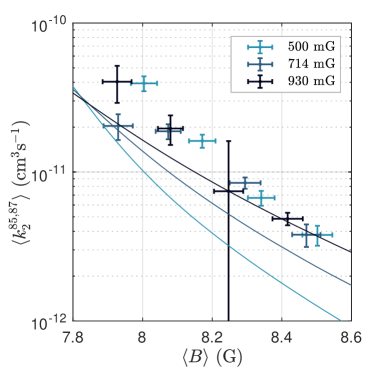
Figure 4: Measurements of $\langle k_{2}^{\mathrm{85,87}}\rangle$ as a function of the average magnetic field $\langle B_{\mathrm{0}}{}\rangle$ for three amplitudes $B_{\mathrm{\rf{}}}$ of a $3.6\text{\,}\mathrm{MHz}$ -dressing field. The solid lines show values of $\langle k_{2}^{\mathrm{85,87}}\rangle$ for each amplitude as predicted from coupled-channel calculations.

IV Quantum scattering calculations

We model the collisional losses by carrying out quantum-mechanical scattering calculations using the MOLSCAT program Hutson and Le Sueur (2019a, b). The method used was described in ref. Owens and Hutson, 2017 for polarization in the plane perpendicular to the magnetic field, and is summarized in appendix:QSC_NumericalMethodseq:Eq. (A)appendix:QSC_NumericalMethodsfig:Fig. Aappendix:QSC_NumericalMethodstab:Table Aappendix:QSC_NumericalMethodsappendix:Appendix Aappendix:QSC_NumericalMethodssec:Section A. It has antecedents in refs. Kaufman et al., 2009; Tscherbul et al., 2010; Hanna et al., 2010. The wave function for a colliding pair of atoms is expanded in an uncoupled -dressed basis set,

$$|s_{1}m_{s1}\rangle|i_{1}m_{i1}\rangle|s_{2}m_{s2}\rangle|i_{2}m_{i2}\rangle|LM_{L}\rangle|NM_{N}\rangle,$$ (17)

where the indices ($1$, $2$) label quantities associated with the first and second atoms, $L$ is the angular momentum for relative motion of the two atoms, and $M_{L}$ is its projection onto the $z$ axis.

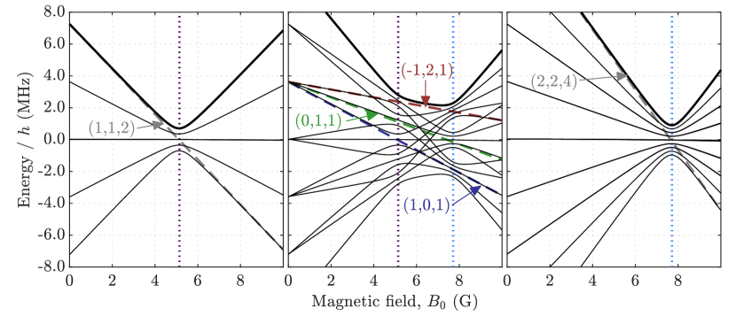
Figure 5: The -dressed atomic thresholds (black, solid) for $\mathrm{{}^{87}Rb}$+$\mathrm{{}^{87}Rb}$ (left), $\mathrm{{}^{87}Rb}$+$\mathrm{{}^{85}Rb}$ (center) and $\mathrm{{}^{85}Rb}$+$\mathrm{{}^{85}Rb}$ (right) for $m_{f1}+m_{f2}+M_{N}=0$, with $B_{\mathrm{\rf{}}}{}=$0.5\text{\,}\mathrm{G}$$ at a frequency of $3.6\text{\,}\mathrm{MHz}$. Both atoms are in their lower hyperfine state. Selected thresholds are also shown for zero intensity (dashed lines), labelled with quantum numbers $(m_{f1},m_{f2},N)$. The resonances for each species are indicated by vertical dotted lines. The thresholds corresponding to collisions of trapped atoms in this work are indicated in bold.

To understand collisions between trapped atoms, it is useful to consider the thresholds (i.e., the energies of separated atomic pairs) as a function of magnetic field. Figure 5 compares the thresholds for $\mathrm{{}^{87}Rb}$+$\mathrm{{}^{85}Rb}$ with those for $\mathrm{{}^{87}Rb}$+$\mathrm{{}^{87}Rb}$ and $\mathrm{{}^{85}Rb}$+$\mathrm{{}^{85}Rb}$ for an field strength $B_{\mathrm{\rf{}}}{}=$0.5\text{\,}\mathrm{G}$$. Only states with $m_{f1}+m_{f2}+M_{N}=0$ are shown; as discussed below, this quantity is conserved in spin-exchange collisions (though not in spin-relaxation collisions).

IV.1 Homonuclear systems

The thresholds for the homonuclear systems are shown in the end panels of fig:Rb2thresheq:Eq. (5)fig:Rb2threshfig:Fig. 5fig:Rb2threshtab:Table 5fig:Rb2threshappendix:Appendix 5fig:Rb2threshsec:Section 5. They show simple maxima or minima at a single magnetic field, $B=$5.12\text{\,}\mathrm{G}$$ for $\mathrm{{}^{87}Rb}$ and $B=7.70$ G for $\mathrm{{}^{85}Rb}$. In all cases the trapped states correspond to the uppermost threshold of those shown, though other thresholds exist for different photon numbers or higher hyperfine states. For $\mathrm{{}^{87}Rb}$+$\mathrm{{}^{87}Rb}$, the uppermost state has character $(m_{f1},m_{f2},N)=(1,1,2)$ at fields below the crossing and $(-1,-1,-2)$ above it. For $\mathrm{{}^{85}Rb}$+$\mathrm{{}^{85}Rb}$, the uppermost state has character $(2,2,4)$ below the crossing and $(-2,-2,-4)$ above it.

In both homonuclear cases, there are no lower-energy states in the same multiplet with the same photon number, so collisional decay can occur in only two ways Owens and Hutson (2017):

(1) Close to the crossing, the $m_{f}$ quantum numbers are mixed by the photon couplings, so that -induced spin-exchange collisions can transfer atoms to lower thresholds without changing $L$ from 0.

(2) At fields above the crossing, the $m_{f}\!=\!-1$ state for $\mathrm{{}^{87}Rb}$ (or $m_{f}\!=\!-2$ state for $\mathrm{{}^{85}Rb}$) is not the ground state. Even in the absence of radiation, two $m_{f}=-1$ or $-2$ atoms can undergo spin-relaxation collisions that change both $M_{F}=m_{f1}+m_{f2}$ and $M_{L}$ (and thus must change $L$ from 0 to 2) but conserve $M_{F}+M_{L}$. Spin relaxation is usually very slow, both because the spin-dipolar coupling $\hat{V}^{\rm d}(R)$ is very weak and because there is a centrifugal barrier higher than the kinetic energy in the outgoing channel with $L=2$.

$\mathrm{{}^{87}Rb}$+$\mathrm{{}^{87}Rb}$ is a special case, with very similar singlet and triplet scattering lengths $a_{\rm s}=$90.6\text{\,}\mathrm{bohr}$$ and $a_{\rm t}=$98.96\text{\,}\mathrm{bohr}$$. This is known to suppress spin-exchange collisions dramatically Myatt et al. (1997); Julienne et al. (1997); Burke et al. (1997), and ref. Owens and Hutson, 2017 showed that it also suppresses -induced spin-exchange collisions. Thus collisional losses in -dressed traps for pure $\mathrm{{}^{87}Rb}$ are dominated by spin relaxation, somewhat modified by the radiation Owens and Hutson (2017). $\mathrm{{}^{85}Rb}$+$\mathrm{{}^{85}Rb}$ has $a_{\rm s}=$2,735\text{\,}\mathrm{bohr}$$ and $a_{\rm t}=$-386\text{\,}\mathrm{bohr}$$ Blackley et al. (2013); although superficially very different, these give similar values of the low-energy s-wave scattering phase. As a result, -free and -induced spin-exchange collisions are suppressed for pure $\mathrm{{}^{85}Rb}$ as well, though not as strongly as for $\mathrm{{}^{87}Rb}$.

IV.2 Heteronuclear systems

The thresholds for $\mathrm{{}^{87}Rb}$+$\mathrm{{}^{85}Rb}$ are very different from those for the homonuclear systems. The uppermost state has character $(m_{f1},m_{f2},N)=(1,2,3)$ at fields below the $\mathrm{{}^{87}Rb}$ resonance at $5.12\text{\,}\mathrm{G}$, and $(-1,-2,-3)$ above the $\mathrm{{}^{85}Rb}$ resonance at $7.70\text{\,}\mathrm{G}$. -induced spin exchange is possible close to the crossings and -modified spin relaxation is possible above $5.12\text{\,}\mathrm{G}$, as for the homonuclear systems. However, at magnetic fields between the two crossings the uppermost state has predominantly $(-1,2,1)$ character, and there are lower pair states that have predominantly $(0,1,1)$ and (1,0,1) character, with the same photon number and value of $M_{F}$, as shown by dashed lines in fig:Rb2thresheq:Eq. (5)fig:Rb2threshfig:Fig. 5fig:Rb2threshtab:Table 5fig:Rb2threshappendix:Appendix 5fig:Rb2threshsec:Section 5. Spin-exchange collisions that transfer atoms to these lower thresholds are thus allowed in this intermediate region, even without the couplings due to radiation. The scattering lengths for $\mathrm{{}^{87}Rb}$+$\mathrm{{}^{85}Rb}$ are $a_{\rm s}=$202\text{\,}\mathrm{bohr}$$ and $a_{\rm t}=$12\text{\,}\mathrm{bohr}$$, so spin exchange is not suppressed in the mixture and fast losses are expected at these intermediate fields.

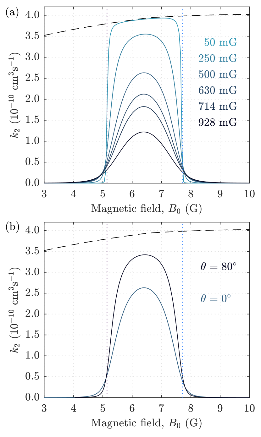
Figure 6: Rate coefficients for inelastic collisions between -dressed $\mathrm{{}^{87}Rb}$ and $\mathrm{{}^{85}Rb}$ atoms in their hyperfine ground states, as a function of magnetic field, at a collision energy of $0.4\text{\,}\mathrm{\SIUnitSymbolMicro K}$. Results are shown for radiation with $\sigma_{-}$ polarization at a frequency of $3.6\text{\,}\mathrm{MHz}$. (a) Dependence on $B_{\mathrm{\rf{}}}$ with polarization in the plane perpendicular to $B_{\mathrm{0}}$. The dashed black line shows the rate coefficient for -free spin exchange for $(f{},m_{f})=\mathrm{{}^{87}Rb}\,(1,-1)+\mathrm{{}^{85}Rb}\,(2,2)$. The dotted lines indicate the magnetic field at which the is resonant for $\mathrm{{}^{85}Rb}$ and $\mathrm{{}^{87}Rb}$. (b) Dependence on the tilt angle $\theta_{\mathrm{}}$, for $B_{\mathrm{\rf{}}}$ fixed at $0.5\text{\,}\mathrm{G}$.

IV.3 Calculated rates and comparison

fig:8785losseq:Eq. (6)fig:8785lossfig:Fig. 6fig:8785losstab:Table 6fig:8785lossappendix:Appendix 6fig:8785losssec:Section 6a shows the calculated inelastic rate coefficients for collisions between -dressed $\mathrm{{}^{87}Rb}$ atoms in $f\!=\!1$, $\widetilde{m}\!=\!1$ and $\mathrm{{}^{85}Rb}$ atoms in $f\!=\!2$, $\widetilde{m}\!=\!2$ as a function of magnetic field, for several field strengths. The calculations were carried out for $\sigma_{-}$ polarization in the plane perpendicular to $B_{\mathrm{0}}$. In these calculations $L_{\rm max}=0$, so spin-relaxation collisions are excluded. At the lowest field strength, $B_{\mathrm{\rf{}}}{}=$50\text{\,}\mathrm{mG}$$, the avoided crossings between the thresholds are very sharp and the states are well described by the quantum numbers $(m_{f1},m_{f2},N)$ introduced at the start of sec:QuantumScatteringCalculationseq:Eq. (IV)sec:QuantumScatteringCalculationsfig:Fig. IVsec:QuantumScatteringCalculationstab:Table IVsec:QuantumScatteringCalculationsappendix:Appendix IVsec:QuantumScatteringCalculationssec:Section IV. In this regime the spin-exchange losses are forbidden below the $\mathrm{{}^{87}Rb}$ radiofrequency resonance at $5.12\text{\,}\mathrm{G}$ and above the $\mathrm{{}^{85}Rb}$ radiofrequency resonance at $7.70\text{\,}\mathrm{G}$, but at intermediate fields they occur at almost the full -free rate for $(f,m_{f})=(1,-1)+(2,2)$ collisions, shown as the black dashed line. At higher field strengths, the avoided crossings extend further into the intermediate field region; the uppermost state is a mixture of $(m_{f1},m_{f2},N)=(-1,2,1)$ and other pair states that do not decay as fast. The effect is to broaden the edges of the flat-topped peak that exists for $B_{\mathrm{\rf{}}}{}=$0.05\text{\,}\mathrm{G}$$ and depress the height of the peak in the central region.

In the experiment, the atoms are trapped at locations where the magnetic field is not perpendicular to the plane of circular polarization. To explore the effects of this, we carried out additional calculations where the radiation is still $\sigma_{-}$ polarized in the plane perpendicular to $z$, but the static magnetic field $B_{0}$ is tilted by an angle $\theta$ from the $z$ axis. In this case $M_{\textrm{tot}}$ is no longer conserved, resulting in an increase in the number of open channels. For $L_{\textrm{max}}=0$, the number of open channels increases from 15 to 56. The calculated loss profiles are shown in fig:8785losseq:Eq. (6)fig:8785lossfig:Fig. 6fig:8785losstab:Table 6fig:8785lossappendix:Appendix 6fig:8785losssec:Section 6b for $B_{\mathrm{\rf{}}}{}=$0.5\text{\,}\mathrm{G}$$ and different values of the tilt angle $\theta$; the profile remains qualitatively similar to that at $\theta=0$, especially far from the avoided crossings in fig:Rb2thresheq:Eq. (5)fig:Rb2threshfig:Fig. 5fig:Rb2threshtab:Table 5fig:Rb2threshappendix:Appendix 5fig:Rb2threshsec:Section 5, where the magnetic field dominates. However, the onset of loss is sharper for tilted fields, resembling that at smaller values of $B_{\mathrm{\rf{}}}$ in fig:8785losseq:Eq. (6)fig:8785lossfig:Fig. 6fig:8785losstab:Table 6fig:8785lossappendix:Appendix 6fig:8785losssec:Section 6a.

At fields above the resonance at $5.12\text{\,}\mathrm{G}$, spin relaxation can also occur. For example the state $(m_{f1},m_{f2},M_{L},N)=(-1,2,0,1)$ can decay to $(0,2,-1,1)$, $(1,2,-2,1)$, $(-1,1,1,1)$ or $(-1,0,2,1)$, conserving $M_{F}+M_{L}$. This spin-relaxation loss is slower than the spin-exchange losses considered in this paper by five orders of magnitude and so is neglected in the analysis.

Overlap-weighted averages $\langle k_{2}^{\mathrm{85,87}}\rangle$ of the calculated rate coefficients $k_{2}^{\mathrm{85,87}}$ are plotted as solid lines alongside the experimental data in fig:k2vBeq:Eq. (4)fig:k2vBfig:Fig. 4fig:k2vBtab:Table 4fig:k2vBappendix:Appendix 4fig:k2vBsec:Section 4. To perform the overlap-weighted averaging, we calculate the spatial distributions $n_{85}$, $n_{87}$ using the average temperature, atom number and trapping fields for each particular value of $B_{\mathrm{\rf{}}}$ shown. We numerically integrate these density distributions to determine $\langle k_{2}^{\mathrm{85,87}}\rangle=\int n_{85}n_{87}k_{2}^{\mathrm{85,87}}dV$, taking into account the variation of $k_{2}^{\mathrm{85,87}}$ with $B_{\mathrm{0}}$. The tilt angle $\theta$ varies by only a few degrees across the region where the two species overlap, and so we use a constant $\theta=$$$ for the calculations.

Our calculated values of $\langle k_{2}^{\mathrm{85,87}}\rangle$ are in reasonable agreement with the experimental measurements shown in fig:k2vBeq:Eq. (4)fig:k2vBfig:Fig. 4fig:k2vBtab:Table 4fig:k2vBappendix:Appendix 4fig:k2vBsec:Section 4. The measurements clearly demonstrate that $\langle k_{2}^{\mathrm{85,87}}\rangle$ increases with magnetic field as the $\mathrm{{}^{85}Rb}$ resonance is approached from the high-field side, which is consistent with the predicted rate coefficients. No clear trend with amplitude is discernible in our measured data, although this would be difficult to observe given our uncertainties. In general, the measured rates are slightly higher than the predicted values. This discrepancy could be caused by a systematic error that underestimates the atom numbers $\mathcal{N}_{85}$ and $\mathcal{N}_{87}$.

V Semiclassical interpretation

Low inelastic loss rates in -dressed potentials were previously measured in experiments using $\mathrm{{}^{87}Rb}$. Those results were interpreted using a semiclassical model Hofferberth et al. (2006); Garraway and Perrin (2016), which we now revisit in light of our work. The model was first introduced in the context of microwave dressing Agosta et al. (1989), and it has also been applied to collisions during evaporative cooling Moerdijk et al. (1996).

Before we discuss the collision model, we first recap the semiclassical picture of an atom in an field. The Hamiltonian of a single atom interacting with a magnetic field is

$$\mathcal{H}_{\text{}}=g_{f}\mu_{\mathrm{B}}{}\vec{f}\cdot\left(B_{\mathrm{\rf{}}}*{}(t)+B_{\mathrm{0}}*{}\right).$$ (18)

The time-dependence is removed by transforming into a frame that rotates with the field, with coordinate axes

$$\vec{e}_{x}{}^{\prime}= \ \vec{e}_{x}\cos(\omega t)+\vec{e}_{y}\sin(\omega t),$$

$$\vec{e}_{z}{}^{\prime}= \ \vec{e}_{z},$$ (19)

followed by making the rotating-wave approximation. The resulting time-independent Hamiltonian is

$$\mathcal{H}_{\text{RWA}}=\hbar\left(\Omega\vec{e}_{x}{}^{\prime}+\delta\vec{e}_{z}{}^{\prime}\right)\cdot\vec{f},$$ (20)

where $\delta$ is the angular frequency detuning and $\Omega$ the resonant Rabi frequency, defined previously. Diagonalising this semi-classical Hamiltonian gives the eigenenergies of an atom in the applied magnetic fields.

$\mathcal{H}_{\text{RWA}}$ is proportional to the dot product of $\vec{f{}}$ with the vector $\vec{V}$,

$$\vec{V}{}=\left(\Omega\vec{e}_{x}{}^{\prime}+\delta\vec{e}_{z}{}^{\prime}\right).$$ (21)

Consequently, the eigenstates of $\mathcal{H}_{\text{RWA}}$ have a well-defined projection $\widetilde{m}$ of $\vec{f{}}$ in the direction of $\vec{V}$. fig:semiclassicaleq:Eq. (7)fig:semiclassicalfig:Fig. 7fig:semiclassicaltab:Table 7fig:semiclassicalappendix:Appendix 7fig:semiclassicalsec:Section 7a shows $\vec{V}$ observed from the laboratory frame, in which it precesses about the static field $B_{\mathrm{0}}$* at the angular frequency $\omega$ and with angle $\Theta_{\mathrm{}}=\arctan(\delta/\Omega)$.

The semiclassical model of -dressed collisions posits that spin exchange does not occur between identical atoms that are in eigenstates of extreme $\widetilde{m}$ Moerdijk et al. (1996); Hofferberth et al. (2006); Garraway and Perrin (2016). When two such atoms collide, their total angular momentum also has a maximum projection along $\vec{V}$, with $\widetilde{M}=\widetilde{m}_{1}+\widetilde{m}_{2}$. In the semiclassical picture, there are no other open channels with the same value of $\widetilde{M}$, thus spin-exchange collisions are forbidden by violation of angular momentum conservation. We stress that these conclusions are incorrect; the semiclassical picture neglects couplings to the field during collisions, and therefore fails to predict the -induced spin exchange described earlier. The rate coefficient for -induced spin exchange is usually large, but this is not the case for either $\mathrm{{}^{87}Rb}$ or $\mathrm{{}^{85}Rb}$; it appears that the low inelastic loss rates observed previously for -dressed $\mathrm{{}^{87}Rb}$ atoms are in agreement with the semiclassical model’s predictions only by coincidence.

The same semiclassical model predicts that spin exchange can occur when two atoms with different values of $|g_{f}|$ collide, even if they are in states of maximum $\widetilde{m}$. The vectors $\vec{V}{}_{85}$, $\vec{V}{}_{87}$ of the two species are in general not parallel, due to the different Rabi frequencies and detunings from the resonance. They precess around $B_{\mathrm{0}}$* at the same angular frequency $\omega$, but with different angles $\Theta_{\mathrm{85}},\Theta_{\mathrm{87}}$. These vectors are illustrated for different $B_{\mathrm{0}}$ in fig:semiclassicaleq:Eq. (7)fig:semiclassicalfig:Fig. 7fig:semiclassicaltab:Table 7fig:semiclassicalappendix:Appendix 7fig:semiclassicalsec:Section 7b, with the associated angles $\Theta_{\mathrm{85}}$ and $\Theta_{\mathrm{87}}$ shown in fig:semiclassicaleq:Eq. (7)fig:semiclassicalfig:Fig. 7fig:semiclassicaltab:Table 7fig:semiclassicalappendix:Appendix 7fig:semiclassicalsec:Section 7c.

At fields much greater than $7.70\text{\,}\mathrm{G}$, the detunings of both species are large and positive. Both angles tend to $\pi/2$, and the vectors $\vec{V}{}_{85}$ and $\vec{V}{}_{87}$ are nearly parallel. In this case, a $\mathrm{{}^{87}Rb}+\mathrm{{}^{85}Rb}$ pair has an extreme value of the total angular momentum $\widetilde{M}$ when each atom is in an eigenstate of maximum $\widetilde{m}{}$. Spin exchange is forbidden on the grounds of angular momentum conservation, as for identical atoms, and the inelastic rate coefficient $k_{2}^{\mathrm{85,87}}$ is small. A similar argument follows for very weak fields below $5.12\text{\,}\mathrm{G}$, where the detunings are large and negative and both $\Theta_{\mathrm{85}}$ and $\Theta_{\mathrm{87}}$ tend to $-\pi/2$.

At intermediate fields, the angles $\Theta_{\mathrm{85}}$ and $\Theta_{\mathrm{87}}$ are very dissimilar. The vectors $\vec{V}{}_{85}$, $\vec{V}{}_{87}$ are misaligned, and spin exchange is not forbidden on grounds of angular momentum conservation. The rate coefficient increases as the angles diverge, and peaks at the midpoint between the two resonances, where $\vec{V}{}_{85}$, $\vec{V}{}_{87}$ are almost antiparallel to each other. The amplitude determines how slowly $\Theta_{\mathrm{85}}$ and $\Theta_{\mathrm{87}}$ change with respect to magnetic field in the vicinity of the resonances, and larger amplitudes therefore broaden the edges of the $k_{2}^{\mathrm{85,87}}$ peak over a wider range of magnetic fields.

Finally, we remark that the semiclassical model predicts that spin exchange occurs for collisions between atoms with $g$-factors of different sign, even when the magnitudes of the $g$-factors are the same; although angles $\Theta_{\mathrm{f=1}}$ and $\Theta_{\mathrm{f=2}}$ are matched, the $\vec{V}$s precesses with different handedness around the static field for each species. Further work is required to compare the semiclassical and quantal pictures with experimental data of different hyperfine states.

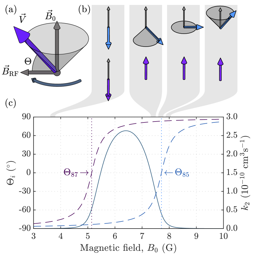
Figure 7: The semiclassical picture. (a) $\vec{V}$ precesses around $B_{\mathrm{0}}$* at the frequency, and is coplanar with both $B_{\mathrm{\rf{}}}$ and $B_{\mathrm{0}}$*. The angle $\Theta_{\mathrm{}}$ is defined in the text. (b) Illustrations of $\vec{V}$ for $\mathrm{{}^{85}Rb}$ (top row) and $\mathrm{{}^{87}Rb}$ (bottom row). Each frame illustrates the fields at different magnetic fields $B_{\mathrm{0}}$. (c) The angle $\Theta_{\mathrm{i}}$ is shown for each species as a function of magnetic field for a $3.6\text{\,}\mathrm{MHz}$ dressing field. Dotted vertical lines mark the resonances for each species. The rate coefficient $k_{2}^{\mathrm{85,87}}$ for $\theta=0$, $B_{\mathrm{\rf{}}}{}=$0.5\text{\,}\mathrm{G}$$ is overlaid for comparison.

VI Conclusion

Mixture	$a_{\mathrm{s}}$ ($\mathrm{bohr}$)	$a_{\mathrm{t}}$ ($\mathrm{bohr}$)	Ref.
$\mathrm{{}^{6}Li}$+$\mathrm{{}^{6}Li}$	$45.154$	$-2113$	Zürn et al. (2013)
$\mathrm{{}^{7}Li}$+$\mathrm{{}^{7}Li}$	$34.331(2)$	$-26.92(7)$	Julienne and Hutson (2014)
$\mathrm{{}^{6}Li}$+$\mathrm{{}^{23}Na}$	$-73(8)$	$-76(5)$	Schuster et al. (2012)
$\mathrm{{}^{7}Li}$+$\mathrm{{}^{39}K}$	$29.83$	$81.99$	Tiemann et al. (2009)
$\mathrm{{}^{7}Li}$+$\mathrm{{}^{40}K}$	$14.88$	$75.27$	Tiemann et al. (2009)
$\mathrm{{}^{7}Li}$+$\mathrm{{}^{41}K}$	$-6.375$	$69.76$	Tiemann et al. (2009)
$\mathrm{{}^{6}Li}$+$\mathrm{{}^{39}K}$	$64.93$	$68.59$	Tiemann et al. (2009)
$\mathrm{{}^{6}Li}$+$\mathrm{{}^{40}K}$	$52.61$	$64.41$	Tiemann et al. (2009)
$\mathrm{{}^{6}Li}$+$\mathrm{{}^{41}K}$	$42.75$	$60.77$	Tiemann et al. (2009)
$\mathrm{{}^{7}Li}$+$\mathrm{{}^{87}Rb}$	$54.75(30)$	$-66.66(10)$	Maier et al. (2015)
$\mathrm{{}^{6}Li}$+$\mathrm{{}^{133}Cs}$	$30.252(100)$	$-34.259(200)$	Repp et al. (2013)
$\mathrm{{}^{7}Li}$+$\mathrm{{}^{133}Cs}$	$45.477(150)$	$908.6(100)$	Repp et al. (2013)
$\mathrm{{}^{23}Na}$+$\mathrm{{}^{23}Na}$	$18.81(80)$	$64.30(40)$	Knoop et al. (2011)
$\mathrm{{}^{23}Na}$+$\mathrm{{}^{39}K}$	$311.8(20)$	$-83.97(50)$	Zhu et al. (2017)
$\mathrm{{}^{23}Na}$+$\mathrm{{}^{40}K}$	$66.7(3)$	$-824.7(30)$	Zhu et al. (2017)
$\mathrm{{}^{23}Na}$+$\mathrm{{}^{41}K}$	$3.39(20)$	$267.05(50)$	Zhu et al. (2017)
$\mathrm{{}^{23}Na}$+$\mathrm{{}^{87}Rb}$	$109$	$70$	Pashov et al. (2005)
$\mathrm{{}^{23}Na}$+$\mathrm{{}^{85}Rb}$	$396$	$81$	Pashov et al. (2005)
$\mathrm{{}^{23}Na}$+$\mathrm{{}^{133}Cs}$	$428(9)$	$30.4(0.6)$	Hood et al. (2019)
$\mathrm{{}^{39}K}$+$\mathrm{{}^{39}K}$	$138.49(12)$	$-33.48(18)$	Falke et al. (2008)
$\mathrm{{}^{39}K}$+$\mathrm{{}^{40}K}$	$-2.84(10)$	$-1985(69)$	Falke et al. (2008)
$\mathrm{{}^{39}K}$+$\mathrm{{}^{41}K}$	$113.07(12)$	$177.10(27)$	Falke et al. (2008)
$\mathrm{{}^{40}K}$+$\mathrm{{}^{40}K}$	$104.41(9)$	$169.67(24)$	Falke et al. (2008)
$\mathrm{{}^{40}K}$+$\mathrm{{}^{41}K}$	$-54.28(21)$	$97.39(9)$	Falke et al. (2008)
$\mathrm{{}^{41}K}$+$\mathrm{{}^{41}K}$	$85.53(6)$	$60.54(6)$	Falke et al. (2008)
$\mathrm{{}^{39}K}$+$\mathrm{{}^{85}Rb}$	$26.5(0.9)$	$63.0(0.5)$	Ferlaino et al. (2006)
$\mathrm{{}^{39}K}$+$\mathrm{{}^{87}Rb}$	$824^{+90}_{-70}$	$35.9(0.7)$	Ferlaino et al. (2006)
$\mathrm{{}^{40}K}$+$\mathrm{{}^{85}Rb}$	$64.5(0.6)$	$-28.4(1.6)$	Ferlaino et al. (2006)
$\mathrm{{}^{40}K}$+$\mathrm{{}^{87}Rb}$	$-111(5)$	$-215(10)$	Ferlaino et al. (2006)
$\mathrm{{}^{41}K}$+$\mathrm{{}^{85}Rb}$	$106.0(0.8)$	$348(10)$	Ferlaino et al. (2006)
$\mathrm{{}^{41}K}$+$\mathrm{{}^{87}Rb}$	$14.0(1.1)$	$163.7(1.6)$	Ferlaino et al. (2006)
$\mathrm{{}^{39}K}$+$\mathrm{{}^{133}Cs}$	$-18.37$	$74.88(9)$	Gröbner et al. (2017)
$\mathrm{{}^{40}K}$+$\mathrm{{}^{133}Cs}$	$-51.44$	$-71.67(45)$	Gröbner et al. (2017)
$\mathrm{{}^{41}K}$+$\mathrm{{}^{133}Cs}$	$-72.79$	$179.06(28)$	Gröbner et al. (2017)
$\mathrm{{}^{85}Rb}$+$\mathrm{{}^{85}Rb}$	$2735$	$-386$	Blackley et al. (2013)
$\mathrm{{}^{85}Rb}$+$\mathrm{{}^{87}Rb}$	$202$	$12$	present work
$\mathrm{{}^{87}Rb}$+$\mathrm{{}^{87}Rb}$	$90.6$	$98.96$	Marte et al. (2002)
$\mathrm{{}^{85}Rb}$+$\mathrm{{}^{133}Cs}$	$585.6$	$11.27$	Cho et al. (2013)
$\mathrm{{}^{87}Rb}$+$\mathrm{{}^{133}Cs}$	$997(11)$	$513.3(2.2)$	Takekoshi et al. (2012)
$\mathrm{{}^{133}Cs}$+$\mathrm{{}^{133}Cs}$	$286.5(1)$	$2858(19)$	Berninger et al. (2013)

Table 1: Singlet $a_{\mathrm{s}}$ and triplet $a_{\mathrm{t}}$ scattering lengths for isotopic mixtures of alkali-metal atoms. The uncertainties have been added where possible.

In this paper we have investigated the inelastic collisions that occur in an -dressed mixture of $\mathrm{{}^{85}Rb}$ and $\mathrm{{}^{87}Rb}$. We measured the loss of a small population of $\mathrm{{}^{85}Rb}$ atoms in the presence of a larger $\mathrm{{}^{87}Rb}$ bath, and identified the dominant mechanism as two-body $\mathrm{{}^{87}Rb}$+$\mathrm{{}^{85}Rb}$ inelastic collisions. The inelastic rate coefficient $k_{2}^{\mathrm{85,87}}$ was shown to vary as a function of magnetic field, with $k_{2}^{\mathrm{85,87}}$ increasing as the atomic resonance was approached from the high-field side. We used a theoretical model of -dressed collisions to predict values of $k_{2}^{\mathrm{85,87}}$, and find they are in reasonable agreement with the measured values given that no free parameters were used to fit.

When -dressed potentials are used to confine atoms, the atoms are in states with a potential energy minimum at the atomic resonance. If two atoms have different magnitudes of $g_{f}$, they are resonant with an applied field at different values of the static field. At fields between these two values, the atoms are predominantly in states where spin-exchange collisions are allowed, even in the absence of coupling to the field. Unless the singlet and triplet scattering lengths are similar, or the magnitudes of both are large, this spin exchange is expected to be fast. This contrasts with the situation when two atoms have very similar values of $g_{f}$, and are thus resonant at the same value of the static field. In this case spin-exchange collisions are forbidden except close to the trap center, where mixing of the Zeeman states by photon interactions permits -induced spin exchange. This -induced spin exchange can also be moderately fast unless the singlet and triplet scattering lengths are similar Owens and Hutson (2017).

tab:ScattLengthseq:Eq. (1)tab:ScattLengthsfig:Fig. 1tab:ScattLengthstab:Table 1tab:ScattLengthsappendix:Appendix 1tab:ScattLengthssec:Section 1 shows the singlet and triplet scattering lengths for different pairs of alkali metal atoms. These values demonstrate that $\mathrm{{}^{87}Rb}$+$\mathrm{{}^{87}Rb}$ is a special case. For most other combinations of alkali-metal isotopes, the singlet and triplet scattering lengths are very different and the rate coefficients for both -induced and -free spin exchange will be large. Although -dressed potentials may enable the manipulation of different isotopes in a mixture Bentine et al. (2017), this paper finds that the dressing will generally cause high rates of inelastic collisions. Nonetheless, there may be some mixtures for which inelastic losses are low. For instance, the combinations $\mathrm{{}^{6}Li}$+$\mathrm{{}^{23}Na}$, $\mathrm{{}^{6}Li}$+$\mathrm{{}^{39}K}$ and $\mathrm{{}^{6}Li}$+$\mathrm{{}^{40}K}$ have similar singlet and triplet scattering lengths, which may suppress interspecies spin exchange. Unfortunately, the singlet and triplet scattering lengths are dissimilar in $\mathrm{{}^{6}Li}$+$\mathrm{{}^{6}Li}$, $\mathrm{{}^{23}Na}$+$\mathrm{{}^{23}Na}$, $\mathrm{{}^{39}K}$+$\mathrm{{}^{39}K}$ and $\mathrm{{}^{40}K}$+$\mathrm{{}^{40}K}$, hence -induced intraspecies spin exchange may be fast for these species. $\mathrm{{}^{87}Rb}$+$\mathrm{{}^{133}Cs}$ may also be interesting; although the interspecies scattering lengths are dissimilar, they are both large and may give rise to similar phase shifts. Furthermore, $\mathrm{{}^{87}Rb}$ and $\mathrm{{}^{133}Cs}$ have different magnitudes of $g_{f}$, allowing species-selective manipulations. It is also well established that $\mathrm{{}^{87}Rb}$+$\mathrm{{}^{87}Rb}$ has low inelastic loss rates when dressed. Further calculations would be required to predict the rate coefficients for a $\mathrm{{}^{87}Rb}$+$\mathrm{{}^{133}Cs}$ mixture.

This paper has not considered inelastic collisions between different hyperfine states of the same isotope, which can also be independently manipulated using -dressed potentials, as was shown for $\mathrm{{}^{87}Rb}$ Navez et al. (2016). The choice of $\mathrm{{}^{87}Rb}$ was fortunate, as the similarity of singlet and triplet scattering lengths suppresses spin-exchange collisions even when such collisions are otherwise allowed Julienne et al. (1997). -dressed potentials have found use for this specific mixture, but our work suggests that this promising technique may be more limited in scope than was previously realized.

Appendix A Numerical methods

We have carried out quantum scattering calculations of collisions between pairs of atoms in -dressed states. The Hamiltonian for the colliding pair is

$$\frac{\hbar^{2}}{2\mu}\left[-R^{-1}\frac{d^{2}}{dR^{2}}R+\frac{\hat{L}^{2}}{R^{2}}\right] +\hat{V}(R)+\hat{h}_{1}+\hat{h}_{2}$$

$$+\hat{h}_{\rm rf}+\hat{h}_{\rm rf,1}^{\rm int}+\hat{h}_{\rm rf,2}^{\rm int},$$ (22)

where $\mu$ is the reduced mass, $\hat{L}^{2}$ is the operator for the end-over-end angular momentum of the two atoms about one another, and $\hat{V}(R)$ is the interaction operator,

$${\hat{V}}(R)=\hat{V}^{\rm c}(R)+\hat{V}^{\rm d}(R).$$ (23)

Here $\hat{V}^{\rm c}(R)=V_{0}(R)\hat{\cal{P}}^{(0)}+V_{1}(R)\hat{\cal{P}}^{(1)}$ is an isotropic potential operator that depends on the electronic potential energy curves $V_{0}(R)$ and $V_{1}(R)$ for the singlet and triplet electronic states and $\hat{V}^{\rm d}(R)$ is a relatively weak anisotropic operator that arises from the combination of spin dipolar coupling at long range and second-order spin-orbit coupling at short range. The singlet and triplet projectors $\hat{\cal{P}}^{(0)}$ and $\hat{\cal{P}}^{(1)}$ project onto subspaces with total electron spin quantum numbers 0 and 1 respectively. The potential curves for the singlet and triplet states of Rb₂ are taken from ref. Strauss et al., 2010.

Expanding the scattering wavefunction in the basis set (17) produces a set of coupled equations in the interatomic distance coordinate $R$. For $\mathrm{{}^{87}Rb}$+$\mathrm{{}^{85}Rb}$ we use a basis set with photon numbers $N$ from $-3$ to 3, $M_{N}=-N$, $L$ restricted to $L_{\rm max}=0$ or 2, and all possible values of $m_{s1}$, $m_{s2}$, $m_{i1}$ $m_{i2}$ and $M_{L}$ that produce the required value of the conserved quantity $M_{\rm tot}=M_{F}+M_{L}+M_{N}$. The resulting number of coupled equations varies from 30 to 478. These equations are solved using the MOLSCAT package Hutson and Le Sueur (2019a, b). In the present work we use the hybrid log-derivative propagator of Alexander and Manolopoulos Alexander and Manolopoulos (1987) to propagate the coupled equations from short range out to $R_{\rm max}=$15,000\text{\,}\mathrm{bohr}$$. At this distance, MOLSCAT transforms the propagated solution into the asymptotic basis set and applies scattering boundary conditions to extract the scattering matrix ${\bf S}$. It then obtains the complex energy-dependent scattering length $a(E,B)=\alpha(E,B)-i\beta(E,B)$ from the identity Hutson (2007)

$$a(E,B)=\frac{1}{ik}\left(\frac{1-S_{00}(E,B)}{1+S_{00}(E,B)}\right),$$ (24)

where $k^{2}=2\mu E/\hbar^{2}$ and $S_{00}(E,B)$ is the diagonal S-matrix element in the incoming s-wave channel. For s-wave collisions (incoming $L=0$), the rate coefficient for inelastic loss is exactly Cvitas̆ et al. (2007)

$$k_{2}(E,B)=\frac{2hg_{\alpha}\beta(E,B)}{\mu\left[1+k^{2}|a(E,B)|^{2}+2k\beta(E,B)\right]},$$ (25)

where $g_{\alpha}$ is 2 for identical bosons and 1 for distinguishable particles. In the present work we evaluated $k_{2}(E,B)$ from scattering calculations at an energy $E=0.4\ \mu{\rm K}\times k_{\rm B}$. We did not carry out explicit energy averaging, since $k_{2}(E,B)$ is independent of energy in the limit $E\rightarrow 0$. We verified the limit holds by performing additional calculations of $k_{2}$ at an energy $E=$5\text{\,}\mathrm{\SIUnitSymbolMicro K}$$, and found that the inelastic rate coefficients vary by only $15\text{\,}\mathrm{\char 37\relax}$ between the two sets of calculations in the field region of the experiments.

References

- Ferrier-Barbut et al. (2014) I. Ferrier-Barbut, M. Delehaye, S. Laurent, A. T. Grier, M. Pierce, B. S. Rem, F. Chevy, and C. Salomon, Science 345, 1035 (2014).
- Cetina et al. (2016) M. Cetina, M. Jag, R. S. Lous, I. Fritsche, J. T. M. Walraven, R. Grimm, J. Levinsen, M. M. Parish, R. Schmidt, M. Knap, and E. Demler, Science 354, 96 (2016).
- DeSalvo et al. (2019) B. J. DeSalvo, K. Patel, G. Cai, and C. Chin, Nature (London) 568, 61 (2019).
- Hohmann et al. (2017) M. Hohmann, F. Kindermann, T. Lausch, D. Mayer, F. Schmidt, E. Lutz, and A. Widera, Phys. Rev. Lett. 118, 263401 (2017).
- Liu et al. (2018) L. R. Liu, J. D. Hood, Y. Yu, J. T. Zhang, N. R. Hutzler, T. Rosenband, and K.-K. Ni, Science 360, 900 (2018).
- Schmidt et al. (2019) F. Schmidt, D. Mayer, Q. Bouton, D. Adam, T. Lausch, J. Nettersheim, E. Tiemann, and A. Widera, Phys. Rev. Lett. 122, 013401 (2019).
- Papp and Wieman (2006) S. B. Papp and C. E. Wieman, Phys. Rev. Lett. 97, 180404 (2006).
- De Marco et al. (2019) L. De Marco, G. Valtolina, K. Matsuda, W. G. Tobias, J. P. Covey, and J. Ye, Science 363, 853 (2019).
- Garraway and Perrin (2016) B. M. Garraway and H. Perrin, J. Phys. B: At. Mol. Opt. Phys. 49, 172001 (2016).
- Perrin and Garraway (2017) H. Perrin and B. M. Garraway, Adv. At., Mol., Opt. Phys. 66, 181 (2017).
- Merloti et al. (2013) K. Merloti, R. Dubessy, L. Longchambon, A. Perrin, P.-E. Pottie, V. Lorent, and H. Perrin, New J. Phys. 15, 033007 (2013).
- Hofferberth et al. (2006) S. Hofferberth, I. Lesanovsky, B. Fischer, J. Verdu, and J. Schmiedmayer, Nature Phys. 2, 710 (2006).
- Harte et al. (2018) T. L. Harte, E. Bentine, K. Luksch, A. J. Barker, D. Trypogeorgos, B. Yuen, and C. J. Foot, Phys. Rev. A 97, 013616 (2018).
- Lesanovsky and von Klitzing (2007) I. Lesanovsky and W. von Klitzing, Phys. Rev. Lett. 99, 083001 (2007).
- Gildemeister et al. (2010) M. Gildemeister, E. Nugent, B. E. Sherlock, M. Kubasik, B. T. Sheard, and C. J. Foot, Phys. Rev. A 81, 031402 (2010).
- Sherlock et al. (2011) B. E. Sherlock, M. Gildemeister, E. Owen, E. Nugent, and C. J. Foot, Phys. Rev. A 83, 043408 (2011).
- Extavour et al. (2006) M. H. T. Extavour, L. J. LeBlanc, T. Schumm, B. Cieslak, S. Myrskog, A. Stummer, S. Aubin, and J. H. Thywissen, AIP Conf. Proc. 869, 241 (2006).
- Navez et al. (2016) P. Navez, S. Pandey, H. Mas, K. Poulios, T. Fernholz, and W. von Klitzing, New J. Phys. 18, 075014 (2016).
- Bentine et al. (2017) E. Bentine, T. L. Harte, K. Luksch, A. J. Barker, J. Mur-Petit, B. Yuen, and C. J. Foot, J. Phys. B: At. Mol. Opt. Phys. 50, 094002 (2017).
- Arimondo et al. (1977) E. Arimondo, M. Inguscio, and P. Violino, Rev. Mod. Phys. 49, 31 (1977).
- Bloch et al. (2001) I. Bloch, M. Greiner, O. Mandel, T. W. Hänsch, and T. Esslinger, Phys. Rev. A 64, 021402 (2001).
- Ockeloen et al. (2010) C. F. Ockeloen, A. F. Tauschinsky, R. J. C. Spreeuw, and S. Whitlock, Phys. Rev. A 82, 061606 (2010).
- Hutson and Le Sueur (2019a) J. M. Hutson and C. R. Le Sueur, Comput. Phys. Commun. 241, 9 (2019a).
- Hutson and Le Sueur (2019b) J. M. Hutson and C. R. Le Sueur, “molscat, bound and field, version 2019.0,” https://github.com/molscat/molscat (2019b).
- Owens and Hutson (2017) D. J. Owens and J. M. Hutson, Phys. Rev. A 96, 042707 (2017).
- Kaufman et al. (2009) A. M. Kaufman, R. P. Anderson, T. M. Hanna, E. Tiesinga, P. S. Julienne, and D. S. Hall, Phys. Rev. A 80, 050701 (2009).
- Tscherbul et al. (2010) T. V. Tscherbul, T. Calarco, I. Lesanovsky, R. V. Krems, A. Dalgarno, and J. Schmiedmayer, Phys. Rev. A 81, 050701 (2010).
- Hanna et al. (2010) T. M. Hanna, E. Tiesinga, and P. S. Julienne, New J. Phys. 12, 083031 (2010).
- Myatt et al. (1997) C. J. Myatt, E. A. Burt, R. W. Ghrist, E. A. Cornell, and C. E. Wieman, Phys. Rev. Lett. 78, 586 (1997).
- Julienne et al. (1997) P. S. Julienne, F. H. Mies, E. Tiesinga, and C. J. Williams, Phys. Rev. Lett. 78, 1880 (1997).
- Burke et al. (1997) J. P. Burke, J. L. Bohn, B. D. Esry, and C. H. Greene, Phys. Rev. A 55, R2511 (1997).
- Blackley et al. (2013) C. L. Blackley, C. R. Le Sueur, J. M. Hutson, D. J. McCarron, M. P. Köppinger, H.-W. Cho, D. L. Jenkin, and S. L. Cornish, Phys. Rev. A 87, 033611 (2013).
- Agosta et al. (1989) C. C. Agosta, I. F. Silvera, H. T. C. Stoof, and B. J. Verhaar, Phys. Rev. Lett. 62, 2361 (1989).
- Moerdijk et al. (1996) A. J. Moerdijk, B. J. Verhaar, and T. M. Nagtegaal, Phys. Rev. A 53, 4343 (1996).
- Zürn et al. (2013) G. Zürn, T. Lompe, A. N. Wenz, S. Jochim, P. S. Julienne, and J. M. Hutson, Phys. Rev. Lett. 110, 135301 (2013).