From Exact Results to Gauge Dynamics on $\mathbb{R}^{3}\times S^{1}$

Abstract

We revisit the vacuum structure of the $\mathcal{N}=1$ Intriligator-Seiberg-Shenker model on $\mathbb{R}^{3}\times S^{1}$. Guided by the Cardy-like asymptotics of its Romelsberger index, and building on earlier semi-classical results by Poppitz and Ünsal, we argue that previously overlooked non-perturbative effects generate a Higgs-type potential on the classical Coulomb branch of the low-energy effective 3d $\mathcal{N}=2$ theory. In particular, on part of the Coulomb branch we encounter the first instance of a dynamically-generated quintic monopole superpotential.

1 Introduction

Some twenty-five years ago, Intriligator, Seiberg, and Shenker (ISS) Intriligator:1994rx published a study of a fascinating $\mathcal{N}=1$ model which has continued to display surprising features ever since. The model is an SU(2) gauge theory, which besides the gauge multiplet only has a single chiral multiplet $Q_{I=3/2}$ transforming in the spin-$3/2$ representation of the gauge group. It is asymptotically free (with the one-loop beta-function coefficient $b=6-5=1$), and has a U(1)_R symmetry under which $Q_{I=3/2}$ has charge $3/5$.

Using holomorphy arguments it was shown that the model, placed on $\mathbb{R}^{4}$, admits a moduli space of SUSY vacua parametrized by the basic gauge-singlet superfield $u=Q_{I=3/2}^{4}$ (with a totally-symmetric contraction of the gauge indices). As for the most interesting point $u=0$ on the moduli space, there used to be two main proposals for its IR behavior: confinement versus non-trivial superconformal fixed-point. The original study Intriligator:1994rx deemed the confinement scenario more likely because of the remarkable $\mathrm{Tr}R$ and $\mathrm{Tr}R^{3}$ ’t Hooft anomaly matchings between the UV constituents and $u$ as the IR superfield. Under the confinement hypothesis, it was shown that dynamical SUSY breaking can be realized by adding a tree-level superpotential.

However, the confinement proposal was subsequently questioned Brodie:1998vv ; Intriligator:2005if , and after several years of suspense eventually ruled out by Vartanov in Vartanov:2010xj . Vartanov’s work is an outstanding example of use of exact results to settle questions in $\mathcal{N}=1$ gauge dynamics. The exact observable employed in Vartanov:2010xj was the Romelsberger index Romelsberger:2005eg , which up to a Casimir-energy factor can be identified with the supersymmetric partition function on $S^{3}\times S^{1}$ Assel:2014paa . The index is known to be RG-invariant. Therefore under the confinement scenario of Intriligator:1994rx it should have matched between the IR superfield $u$ and the UV fields of the ISS model; explicit computation found otherwise Vartanov:2010xj .

Closely related is the dynamics of the ISS model on $\mathbb{R}^{3}\times S^{1},$ with periodic spin structure on the circle. It has been studied by Poppitz and Ünsal Poppitz:2009kz with the motivation to approach the $\mathbb{R}^{4}$ behavior via an adiabatic argument by varying the radius $r_{S^{1}}$ of the circle. Their results include a description of the vacua on $\mathbb{R}^{3}\times S^{1}.$ In particular, it was suggested in Poppitz:2009kz that the moduli space of vacua on $\mathbb{R}^{3}\times S^{1}$ contains a new flat direction, namely a compact Coulomb branch (for the low-energy effective 3d $\mathcal{N}=2$ theory living on $\mathbb{R}^{3}$) parametrized by a periodic holonomy variable related to the component of the 4d gauge field along the circle.

In the present paper we employ the Romelsberger index to clarify the low-energy dynamics of the ISS model on $\mathbb{R}^{3}\times S^{1}.$ Specifically, our study is motivated by the finding in Ardehali:2015bla that the asymptotic behavior of the Romelsberger index of the model, as $r_{S^{3}}\to\infty$, exhibits a non-trivial potential for the holonomy variable (see Figure 1). In light of this result, and building on earlier semi-classical developments due to Poppitz and Ünsal, we re-examine the arguments and conclusions of Poppitz:2009kz regarding the compactified ISS model.

Below, by the “low-energy” regime on $\mathbb{R}^{3}\times S^{1}$ we mean the regime where energies are much smaller than $1/r_{S^{1}}$. Whenever performing semi-classical analysis, we moreover assume that $r_{S^{1}}\Lambda_{\mathrm{ISS}}\ll 1$, with $\Lambda_{\mathrm{ISS}}$ the dynamical scale of the model. In such low-energy, semi-classical regimes, a Kaluza-Klein (KK) reduction on the circle gives a finite number of fields that are massless on $\mathbb{R}^{3}$ and constitute the dynamical degrees of freedom, together with infinite towers of massive KK modes that ought to be integrated out.

Our main results are as follows. Firstly, at the classical level, we carefully identify the fields that are massless in the three-dimensional sense. We find that the mixture of KK charge and gauge charge leads to extra massless fields on the classical Coulomb branch. This leads to a new picture of the classical moduli space (see Figure 2). Secondly, at the semi-classical level, we find a monopole-induced potential on the classical Coulomb branch (see (8)) which has the same qualitative profile as the holonomy potential arising from the $r_{S^{3}}\to\infty$ limit of the Romelsberger index! This monopole-induced potential has the effect of lifting the parts of the classical Coulomb branch that are away from the loci supporting charged massless 3d fields.

We emphasize that our use of the index in addressing gauge dynamics on $\mathbb{R}^{3}\times S^{1}$ is not as direct as Vartanov’s use of it in Vartanov:2010xj . Rather, we utilize (the asymptotics of) the index as a guide for a subsequent careful semi-classical analysis, and it is the latter that yields our main results. While it is intuitively expected that the $r_{S^{3}}\to\infty$ limit of the index might encode semi-classical dynamics on $\mathbb{R}^{3}\times S^{1}$, the details of the connection are somewhat mysterious at the moment; in particular, the asymptotics of the index yields a potential for the holonomy which is piecewise linear, whereas the semi-classical (multi-)monopole potential on $\mathbb{R}^{3}\times S^{1}$ is piecewise exponential, and the relation between the two is far from clear. We will comment more on this point in section 5.

The rest of this paper is organized as follows. In section 2 we explain how the leading asymptotics of the Romelsberger index might be used as a guide for studying semi-classical gauge dynamics on $\mathbb{R}^{3}\times S^{1}.$ In section 3 we perform a careful semi-classical analysis of the low-energy dynamics of the compactified ISS model. In section 4 we make some preliminary remarks on the IR phase of the low-energy effective 3d $\mathcal{N}=2$ theory. In section 5 we put our results in a wider context and also comment on a few related open problems. Appendix A discusses the physical content of the subleading asymptotics of the index, while appendix B discusses an alternative perspective on the piecewise-linear potential arising in the leading asymptotics.

2 The index perspective

In this section we present intuitive arguments (as in section 5.4 of Ardehali:2015bla ) which will guide our semi-classical analysis in the next section.

We approach $\mathbb{R}^{3}\times S^{1}$ by taking the large-$r_{S^{3}}$ limit of $S^{3}\times S^{1}$. The partition function on the latter space is called the Romelsberger index Romelsberger:2005eg , and can be computed exactly for any $\mathcal{N}=1$ gauge theory with a U($1$)_R symmetry. Focusing on non-chiral theories with semi-simple gauge group for simplicity, the asymptotics of the index as the radius of the $S^{3}$ is sent to infinity takes the form Ardehali:2015bla ; Rains:2009 ; Ardehali:2016kza

$$\mathcal{I}(\beta)\approx\mathrm{e}^{-\mathcal{E}^{\mathrm{DK}}_{0}(\beta)}\int_{\mathfrak{h}_{cl}}\mathrm{e}^{-\frac{4\pi^{2}}{\beta}L_{h}(\boldsymbol{x})}\,\mathrm{d}^{r_{G}}{x}\qquad(\text{as }\beta\to 0),$$ (1)

where $\beta=2\pi r_{S^{1}}/r_{S^{3}}$, and $\mathcal{E}^{\mathrm{DK}}_{0}(\beta)=\frac{\pi^{2}}{3\beta}\mathrm{Tr}R$ is the piece studied by Di Pietro and Komargodski in DiPietro:2014bca . The symbol $\boldsymbol{x}$ stands for the collection $x_{1},\dots,x_{r_{G}}$ parametrizing the unit hypercube in the Cartan subalgebra of the gauge group, whose rank is denoted $r_{G}$; the unit hypercube is denoted by $\mathfrak{h}_{cl}$. (Note that the range of the integration variables $x_{j}$ is kept fixed, e.g. from $-1/2$ to $1/2$, as $\beta\to 0$.) The exponential function $z_{j}=\mathrm{e}^{2\pi ix_{j}}$ maps $\mathfrak{h}_{cl}$ to the moduli space of the eigenvalues of the holonomy matrix $P\exp(i\oint_{S^{1}}A_{4})$, with $A_{4}$ the component of the gauge field $A$ along the $S^{1}$. The integral in (1) is thus over the “classical” moduli space of the holonomies around the circle; hence the subscript $cl$ in $\mathfrak{h}_{cl}$. When $S^{3}$ decompactifies to $\mathbb{R}^{3}$, this moduli space becomes a middle-dimensional section of the classical Coulomb branch of the low-energy effective 3d $\mathcal{N}=2$ theory living on $\mathbb{R}^{3}$; the rest of the classical Coulomb branch is parametrized by the dual photons (see e.g. Aharony:2013dha ), which the index does not see.

Two questions might arise at this stage. First, why is the $\beta\to 0$ limit thought of as decompactifying the $S^{3}$, rather than shrinking the $S^{1}$? Second, what are the asymptotic boundary conditions that our approach via decompactification of the $S^{3}$ imposes on various fields at the infinity of the limiting $R^{3}$? The answer to the first question is that both perspectives are valid: in the body of the paper we are mainly interested in the “crossed-channel” perspective where $\beta\to 0$ is thought of as $r_{S^{3}}\to\infty$, while in the two appendices and parts of section 5 the “direct-channel” perspective, where $\beta\to 0$ is thought of as $r_{S^{1}}\to 0$, will also be discussed. A thorough answer to the second question is beyond the scope of the heuristic arguments of the present section; we only note that to have a correspondence with the index the component of the gauge field along the circle must approach a constant matrix, whose holonomy eigenvalues would be in correspondence with the $z_{j}$ above.

Continuing our study of the index we observe that the integral in (1) localizes in the “Cardy-like limit” $\beta\to 0$ to the minima of the Rains function

$$\begin{split}L_{h}(\boldsymbol{x}):=\frac{1}{2}\sum_{\chi}(1-r_{\chi})\sum_{\rho^{\chi}\in\Delta_{\chi}}\vartheta(\rho^{\chi}\cdot\boldsymbol{x})-\sum_{\alpha_{+}}\vartheta(\alpha_{+}\cdot\boldsymbol{x}),\end{split}$$ (2)

which, as in Ardehali:2015bla , we would like to intuitively interpret as a quantum effective potential on the classical Coulomb branch of the low-energy effective 3d $\mathcal{N}=2$ theory on $\mathbb{R}^{3}$. In Eq. (2) the set of weights of the gauge-group representation of the chiral multiplet $\chi$ is denoted by $\Delta_{\chi}$, and the positive roots of the gauge group by $\alpha_{+}$. The function $\vartheta(x)$ in (2) is defined following Rains as Rains:2009

$$\vartheta(x):=\{x\}(1-\{x\}),$$ (3)

with $\{x\}:=x-\lfloor x\rfloor$ the fractional-part function, defined via the more familiar floor function $\lfloor x\rfloor:=\mathrm{max}\{m\in\mathbb{Z}\ |\ m\leq x\}$. Note that while $\vartheta(x)$ is piecewise quadratic, the Rains function $L_{h}(\mathbf{x})$ is piecewise linear thanks to the U($1$)_R ABJ anomaly cancelation.

With the above reasoning we are led to expect that the minima of the Rains function encode the vacua of the gauge theory on $\mathbb{R}^{3}\times S^{1}$. Of course any non-trivial vacuum structure due to the dual photons would be invisible in this approach, as the index is blind to them. Moreover, any non-trivial Higgs branch of the 3d $\mathcal{N}=2$ theory would also escape this approach, because for any finite $r_{S^{3}}$ the curvature couplings lift them.

Let us now illustrate this connection between the Rains function and the $\mathbb{R}^{3}\times S^{1}$ vacua in a few concrete examples. A particularly simple example is that of SU($N$) SQCD, with enough matter multiplets—namely $N_{f}>N$—so that it has a well-defined U(1)_R symmetry and hence a well-defined index. It is a result essentially due to Rains that in this case a certain generalized triangle inequality (proven in Rains:2009 ) involving $\vartheta(\cdot)$ establishes that the Rains function (2) is minimized when all $x_{j}$ are zero (c.f. section 3.1.1 of Ardehali:2015bla ). This suggests that the theory on $\mathbb{R}^{3}\times S^{1}$ has its classical Coulomb branch lifted by quantum corrections, and only a zero-dimensional space of vacua survives at the quantum level. This is in perfect agreement with the semi-classical analysis of the model as discussed in Aharony:2013dha . Similar remarks apply to USp($2N$) SQCD, which hence furnishes another simple example.

A more nontrivial illustration is provided by SO($N$) SQCD. For concreteness we focus on the theory with SO($2N+1$) gauge group. (Analogous comments apply to the theory with SO($2N$) gauge group.) Again we assume enough matter multiplets—namely $N_{f}>2N-1$—so that there is a well-defined U(1)_R and an index. Then, a rather non-trivial identity (presented in Eq. (3.51) of Ardehali:2015bla ) involving $\vartheta(\cdot)$ establishes that the Rains function is minimized when one—and only one—of the $x_{j}$ is non-zero and the rest are zero (see section 3.2.1 of Ardehali:2015bla ). This one-dimensional space of quantum vacua is again in complete accord with the semi-classical analysis of the $\mathbb{R}^{3}\times S^{1}$ dynamics of the model as discussed in Aharony:2013dha .

For many theories the vacua on $\mathbb{R}^{3}\times S^{1}$ have not yet been studied but the structure of the locus of minima of the Rains function is understood. In such cases the index perspective leads to conjectures regarding the structure of vacua on $\mathbb{R}^{3}\times S^{1}$. In section 5.4 of Ardehali:2015bla such conjectures were put forward for all SU($N$) $ADE$ SQCD Intriligator:2003mi and the Pouliot theories Pouliot:1995zc —in the appropriate range of their parameters such that all their R-charges are in $]0,2[$—as well as for the $\mathbb{Z}_{3}$ orbifold of the SU($N$) $\mathcal{N}=4$ theory. (Some cases with enhanced supersymmetry were also discussed in Ardehali:2015bla on which we comment in section 5 where possible obstructions to the heuristic arguments of the present section are also outlined.)

The case of main interest in the present paper is the ISS model, to which we now turn. In terms of $x:=x_{1}$, the Rains function of the model reads

$$\begin{split}L^{\mathrm{ISS}}_{h}(x)=\frac{2}{5}\vartheta(x)+\frac{2}{5}\vartheta(3x)-\vartheta(2x),\end{split}$$ (4)

and looks like a Mexican hat as in Figure 1.

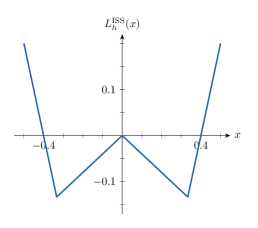
Figure 1: The Rains function of the SU(2) ISS model. Its minima lie at $x=\pm 1/3$.

Following the intuitive line of argument advocated above, Figure 1 would suggest that the quantum vacuum of the ISS model on $\mathbb{R}^{3}\times S^{1}$ lies at $x=1/3$ (which is Weyl-equivalent to $x=-1/3$). As pointed out in Ardehali:2015bla , this appears to be in conflict with an earlier semi-classical analysis of the compactified ISS model by Poppitz and Ünsal Poppitz:2009kz . We now proceed to argue that the analysis of Poppitz and Ünsal, once extended slightly further, actually reveals non-perturbative effects generating a Higgs-type potential qualitatively compatible with Figure 1.

3 Revisiting the semi-classical analysis

We begin our semi-classical analysis with a brief discussion of the perturbative vacuum moduli space of the compactified ISS model. We assume $1/r_{S^{1}}\gg\Lambda_{\mathrm{ISS}}$, so that a semi-classical analysis is reliable in appropriate regions of the classical moduli space.

At energies well below the compactification scale $1/r_{S^{1}}$, semi-classically we have an effective 3d $\mathcal{N}=2$ theory. The scalar in the 3d $\mathcal{N}=2$ vector multiplet comes from the holonomy of the 4d gauge field as follows. Since the gauge group is SU(2), the two eigenvalues of $P\exp(i\oint_{S^{1}}A_{4})$ are of the form $z^{\pm 1}$, and picking one of them as $z$ we can define a periodic scalar $x$ through $z=e^{2\pi ix}$; of course there is a Weyl redundancy in picking one of the two eigenvalues as $z$, and throughout the rest of this paper we fix this redundancy in our scalar by taking $x\in[0,1/2]$. There is no tree-level potential for this scalar, so it parametrizes what is called the classical Coulomb branch of the 3d $\mathcal{N}=2$ theory. Actually, for any $x$ strictly inside the $[0,1/2]$ interval, the super-Higgs mechanism breaks the SU($2$) gauge group down to U($1$), and the 3d photon can be Hodge-dualized to a compact scalar $a$, which also does not have a tree-level potential, and hence combines with $x$ to parametrize the full classical Coulomb branch.

The Coulomb-branch parameter $x$ also determines the real mass of the 3d descendants of the 4d fields that are charged under the Cartan of the gauge group. The chiral multiplet $Q_{I=3/2}$ contains fields with charges $-3,-1,+1,+3$ under the Cartan of the SU($2$). To find the real masses of their 3d descendants we first note that the $m$th KK mode of a 4d field with charge $n$ under the Cartan has real mass $(nx+m)/r_{S^{1}}$; picking the $m\in\mathbb{Z}$ that minimizes the absolute value of this real mass, we get the real mass of the “lightest” among all the KK modes—which we refer to as the 3d descendant.

At $x=0$ all fields yield massless 3d descendants with KK charge $m=0$ of course. Since the descendants $q_{I=3/2}$ of the chiral multiplet have no tree-level potential at $x=0$, we have a classical Higgs branch there parametrized by the gauge-invariant combination $u\sim q_{I=3/2}^{4}$.

More interestingly, we see that the $x=1/3$ point also supports massless 3d fields; these are the descendants of the fields with charges $+3,-3$ inside the chiral multiplet, and we denote them by $q_{+3},q_{-3}$. (Note that $q_{\pm 3}$ have KK charges $m=\mp 1.$) These 3d fields also lack a tree-level potential, and thus yield a classical Higgs branch at $x=1/3$, which can be parametrized by the gauge-invariant combination $M\sim q_{+3}q_{-3}$.

Finally, at $x=1/2$ only the 4d vector multiplet yields massless descendants. The descendants of the 4d gauge multiplet (which have gauge charges $\pm 2$ and KK charges $\mp 1$) restore the SU($2$) gauge group at this point, so we have a 3d pure $\mathcal{N}=2$ SYM sitting there.

Note that both at $x=0$ and at $x=1/2$ the enhanced SU($2$) is recovered. At these points the dual photon $a$ ceases to make sense. In fact even in proximity of these points—in neighborhoods that we suspect to be more precisely of size $\mathcal{O}(r_{S^{1}}\Lambda_{\mathrm{ISS}})$ and $\mathcal{O}(r_{S^{1}}\Lambda_{\mathrm{SYM}})=\mathcal{O}((r_{S^{1}}\Lambda_{\mathrm{ISS}})^{1/6})$ respectively—we expect our semi-classical techniques to lose reliability.

We have now almost completely explained Figure 2. The one remaining feature, namely the pinches at $x=0,1/3,1/2$, are due to the perturbative running of the gauge coupling, which sets the radius of the dual photon; this radius shrinks near points where charged fields become massless—see Strassler:2003qg for a clear exposition.

Figure 2: The perturbative vacuum moduli space of the compactified ISS model. The cones represent the classical Higgs branches. The perturbative Coulomb branch shrinks near the points $x=0,1/3,1/2$ where charged fields become massless. The red neighborhoods are where strong-coupling effects are expected to undermine semi-classical techniques.

No further perturbative effects are expected to modify the vacuum structure (because of the perturbative non-renormalization theorems in particular), so we now turn to the non-perturbative effects.

There are known semi-classical, non-perturbative effects on $\mathbb{R}^{3}\times S^{1}$ due to BPS (anti-) monopoles Gross:1980br and KK (anti-) monopoles Lee:1997vp ; Kraan:1998pm . These can be described in terms of a low-energy monopole superfield.

For SU($2$) gauge group, inside the classical Coulomb branch parametrized by $x(=x_{1})\in(0,1/2)$, and away from pinch-points and the end-points of the interval, the (lowest component of the) monopole superfield takes the form Affleck:1982as

$$Y\sim\exp\left(\frac{2x}{\hat{g}^{2}}\right),$$ (5)

with $\hat{g}^{2}=g^{2}/8\pi^{2}$ and $g$ the gauge coupling. (We have suppressed the dual photon for simplicity; restoring it would only give $Y$ a phase, and leave the modulus as in (5). See Aharony:2013dha for a recent, clear exposition of the relevant basics.) Note however that in $\mathcal{O}(g^{2})$ neighborhoods of pinch-points and the end-points of the interval, quantum-mechanical effects are expected to modify the semi-classical relation (5) between $x$ and $Y$ Aharony:1997bx ; Dorey:1998kq .

An $n$-BPS-monopole effect may contribute $1/Y^{n}$ to the low-energy superpotential Affleck:1982as ; Dorey:1998kq on $\mathbb{R}^{3}\times S^{1}$, and an $m$-KK-monopole effect may contribute $(\eta Y)^{m}$, where $\eta=\mathrm{e}^{-1/\hat{g}^{2}}$ is the 4d instanton factor. (Incidentally, a 4d SU($2$) instanton is often thought of as a composite configuration made out of a BPS and a KK monopole: $\frac{1}{Y}\times\eta Y=\eta$.)

For such multi-monopoles to actually contribute to the low-energy superpotential though, it is necessary that they have precisely two fermionic zero-modes Affleck:1982as . The BPS and the KK monopole both have precisely two gaugino zero-modes, so in absence of chiral multiplets (i.e. in pure SU($2$) SYM) they both contribute to the superpotential, which hence reads $1/Y+\eta Y$. In the ISS model we have to take into account the extra zero-modes arising from the chiral multiplet in the spin-$3/2$ representation of the gauge group. These zero-modes are counted by the following index theorem, given by Poppitz and Ünsal in Poppitz:2008hr (see also Nye:2000eg ):

$$I^{\mathrm{BPS}}_{3/2}=10-I^{\mathrm{KK}}_{3/2}=-3\lfloor-3x\rfloor-\lfloor-x\rfloor+\lfloor x\rfloor+3\lfloor 3x\rfloor.$$ (6)

As indicated in Poppitz:2008hr (below its Eq. (3.10)), the above index theorem implies that for $0<x<1/3$ there are 4 BPS zero-modes—thus 6 KK zero-modes, while for $1/3<x<1/2$ there are 10 BPS zero-modes—hence no KK zero-modes.

It appears like in their later paper Poppitz:2009kz , Poppitz and Ünsal did not consider the range $1/3<x<1/2$. Since in this range the chiral multiplet of the ISS model has no fermionic zero-modes on a KK-monopole background, there should be an $\eta Y$ superpotential generated on this part of the classical Coulomb branch of the model. This superpotential yields a potential which increases with increasing $Y$, and hence with increasing $x$; therefore its qualitative behavior is compatible with the Rains function of the ISS model in that range—c.f. Figure 1!

What about the range $0<x<1/3$? As the index theorem shows, both the BPS and the KK monopole have too many zero-modes to generate a superpotential there. At this point, a result of Poppitz and Ünsal can crucially guide us further Poppitz:2009kz : they found that in the range $0<x<1/3$ the monopole superfield $Y$ has U($1$)_R charge $-2/5$. Thus the natural candidate for a superpotential term would be $1/Y^{5}$, signaling a five-BPS-monopole effect. At first glance it seems like such a term is forbidden because a five-BPS-monopole background would have $5\times 4=20$ chiral-multiplet zero-modes and $5\times 2=10$ gaugino zero-modes—far too many. However, we now argue that the extra zero-modes are not protected by any symmetry, so are expected to be lifted by quantum effects! In particular, because the U($1$)_R charge of the chiral-multiplet fermions is $3/5-1=-2/5$ and that of the gauginos is $+1$, the 20 chiral-multiplet zero-modes can combine with 8 of the gauginos and be lifted without violating U($1$)_R; the corresponding vertex $\psi^{20}\lambda^{8}$ has U($1$)_R-charge $20\times(-2/5)+8\times(+1)=0$, so is not prohibited by any symmetry, and should therefore “naturally”—in the technical sense—be generated. We hence propose that the low-energy Kähler potential arising from the supersymmetric sigma model on the moduli space of a five-BPS-monopole configuration has such a vertex, or actually the more fundamental $\psi^{10}\lambda^{4}$ vertex which would also do the job of soaking up the extra zero-modes (c.f. section 3 of Gauntlett:1995fu pertinent to an analogous four-dimensional situation). The vertex presumably couples the fermion zero-modes to some power of the curvature tensor of the index bundle Manton:1993aa over the five-monopole moduli space (c.f. the last term in Eq. (3.8) of Gauntlett:1995fu ).

Although our proposed mechanism for lifting of the extra zero-modes might appear contrived, in fact several effects of similar nature have already been observed both in three and four dimensions, with various amounts of supersymmetry—see e.g. Gauntlett:1995fu ; Dorey:1997ij ; Dorey:1998kq ; Dorey:1999sj . For the sceptic readers we point out that the non-perturbative two-instanton vertex (c.f. Poppitz:2009kz )

$$\mathrm{e}^{-2S_{\mathrm{inst}}}\psi^{20}\lambda^{8},$$ (7)

also does the job of lifting the extra zero-modes via Kähler corrections; absent the perturbative vertex of the previous paragraph, the vertex (7) would lead to a five-monopole effect suppressed by an $\eta^{2}=\mathrm{e}^{-2S_{\mathrm{inst}}}$ factor, but that suppression would not significantly modify our discussion below.

We conclude that a quintic monopole-superpotential of the form $1/Y^{5}$ is indeed generated over the range $0<x<1/3$ of the classical Coulomb branch. This potential decreases with increasing $x$; therefore its qualitative behavior is compatible with the Rains function of Figure 1 in that range! (Some similar higher-power monopole superpotentials have been recently used in Benini:2017dud ; Amariti:2018gdc ; Amariti:2019rhc —though only up to quadratic degree.)

It is useful—for holomorphy arguments in particular—to employ different Coulomb-branch operators on different sides of the pinch-points. Thus for $x>1/3$ instead of $Y$ we may use $Y^{\prime}_{+}\sim\exp\left(\frac{2x^{\prime}}{\hat{g}^{2}}\right)$, with $x^{\prime}:=x-1/3$. At the quantum-mechanical level we expect $Y^{\prime}_{+}$ to have the nice property that $Y^{\prime}_{+}\to 0$ as $x^{\prime}\to 0^{+}$ Aharony:1997bx . On the other hand, on a neighborhood to the left of $x=1/3$, the Coulomb-branch operator $Y^{\prime}_{-}\sim\exp\left(-\frac{2x^{\prime}}{\hat{g}^{2}}\right)$, proportional to $1/Y$, becomes useful as we expect that quantum-mechanically $Y^{\prime}_{-}\to 0$ as $x^{\prime}\to 0^{-}$. Therefore we can summarize our findings in this section by writing the low-energy superpotential on the classical Coulomb branch of the ISS model on $\mathbb{R}^{3}\times S^{1}$ as

$$W\propto\begin{cases}Y^{\prime 5}_{-}&0<x<1/3,\\ Y^{\prime}_{+}&1/3<x<1/2.\end{cases}$$ (8)

This superpotential—previously thought to be zero—is the main result of the present paper.

Over the range $0<x<1/3$ we argued that a vertex of the form $\psi^{20}\lambda^{8}$ (or two vertices of the form $\psi^{10}\lambda^{4}$) should naturally lift the extra fermionic zero-modes of a five-BPS-monopole background. For $1/3<x<1/2$ we simply used an earlier result of Poppitz and Ünsal Poppitz:2008hr that the KK-monopole background does not have extra fermionic zero-modes. In particular, the semi-classical vacuum structure implied by the low-energy superpotential (8) is compatible with that suggested by the Rains function (4) shown in Figure 1.

Note that the superpotential (8) is useful only outside a small neighborhood of $x=1/3$ wherein new light states associated with $q_{\pm 3}$ appear. However, the superpotential seems to drive the theory to a vacuum in that small neighborhood. The nature of this vacuum is not entirely clear to us, and we will only present some preliminary comments on it in the next section.

It might be possible that a perspective from Seiberg-Witten theory Seiberg:1996nz (see also Aharony:1997bx ) can shed further light on the above picture once the ISS model is embedded in the $\mathcal{N}=2$ $I^{\ast}_{1}$ theory of Argyres:2010py ; Argyres:2015ffa . This approach is currently under investigation.

4 The low-energy phase

In this section we make some rudimentary remarks concerning the low-energy phase, arguing in particular that the theory has a supersymmetric, gapless vacuum. A more careful, conclusive study is left for future work.

First, following the conventional wisdom we assume that the red neighborhoods of the $x=0,1/2$ points, although not really amenable to semi-classical analysis, presumably contain no acceptable vacua because in their semi-classical vicinity the low-energy effective potential is repulsive—c.f. the case of 3d pure $\mathcal{N}=2$ SYM for instance Aharony:1997bx . Hence below we discuss only the vacuum structure near $x=1/3$.

The SU($2$) gauge group is broken down to U($1$) of course. Moreover, of the four components of the chiral multiplet $Q_{I=3/2}$, having U($1$) charges $-3,-1,+1,+3$, the two with charges $-1,+1$ do not yield massless 3d descendants near $x=1/3$. In the resulting low-energy theory we are thus left with the field content of 3d $\mathcal{N}=2$ SQED with chiral multiplets $q_{-3},q_{+3}$ of charge $-3,+3$ coming from the KK modes $\pm 1$ of their 4d parents. This is in fact compatible with the subleading Cardy-like asymptotics of the Romelsberger index of the model as described in appendix A.

It is important to note that the field content discussed in the previous paragraph, and the effective SQED predicated on it, provide a useful description only up to a cut-off scale (or “threshold”)

$$\Lambda^{\mathrm{3d\ SQED}}_{\mathrm{uv}}=\frac{\epsilon}{r_{S^{1}}},$$ (9)

with some $\epsilon\ll 1$. That is to say we consider this SQED as an effective description of only an $\mathcal{O}(\epsilon)$ neighborhood of the pinch at $x^{\prime}(:=x-1/3)=0$. Outside this $\mathcal{O}(\epsilon)$ neighborhood—and away from the red regions—the U(1) gauge theory of the previous section (with the superpotential deformation (8)) provides the appropriate effective description.

In this SQED theory near $x=1/3$, there are no FI or Chern-Simons terms induced through one-loop effects, because the massive fields come in pairs of opposite charge under the low-energy U($1$) gauge group. Non-perturbative effects presumably cannot induce a properly quantized Chern-Simons level either, but since FI parameters need not be quantized we leave open the possibility of an instanton-induced FI parameter $\zeta$. (As we will discuss in appendix A, the subleading $\beta\to 0$ asymptotics of the $S^{3}\times S^{1}$ partition function signals an induced ‘imaginary FI parameter’, which we will explain in that appendix from the $r_{S^{1}}\to 0$ perspective via “high-temperature” perturbative effects; it is the possibility of an induced FI parameter from the $\mathbb{R}^{3}\times S^{1}$ perspective via “low-energy” non-perturbative effects that we are leaving open.)

We expect that the near-pinch SQED inherits a superpotential of the form (8), which would lift its Coulomb branch. In fact one might also expect an extra term of the form $M{Y^{\prime}}_{-}^{1/3}{Y^{\prime}}_{+}^{1/3}$ to be generated dynamically in the theory, since it has the right R-charge: recalling that $q_{\pm 3}$ have R-charge $3/5$, the R-charge of $M\sim q_{+3}q_{-3}$ becomes $6/5$, while those of $Y^{\prime}_{-,+}$ follow from (8) to be $2/5,2$, therefore $M{Y^{\prime}}_{-}^{1/3}{Y^{\prime}}_{+}^{1/3}$ has R-charge $6/5+2/15+2/3=2$. Hence we propose

$$W_{\mathrm{SQED}}\sim M{Y^{\prime}}_{-}^{1/3}{Y^{\prime}}_{+}^{1/3}+Y^{\prime 5}_{-}+Y^{\prime}_{+},$$ (10)

wherein $Y^{\prime}_{+},Y^{\prime}_{-},M$ ought to be considered independent operators. We now proceed to present independent arguments supporting a slightly more refined version of (10), given in (16).

A point we need to establish here is that the near-pinch SQED not only has extra massless fields compared to the effective U(1) theory outside the $\mathcal{O}(\epsilon)$ neighborhood, it also has different monopole operators. This is seen from the following discussion.

Recall that the chiral multiplet $Q_{I=3/2}$ yields states of charge $-3,-1,+1,+3$ on the Coulomb branch. However, because the states of charge $\pm 1$ have masses $\geq 1/3r_{S^{1}}$, they lie far beyond the SQED cut-off $\epsilon/r_{S^{1}}$. Therefore we need not worry about their quantization in the near-pinch SQED. It is only the electric sources with charge $\pm 3$ that have to satisfy a Dirac quantization condition with respect to the monopoles, implying that the minimal allowed magnetic charge is $\pm 1/3$. The minimal-flux monopole operators of the near-pinch SQED hence read (c.f. Aharony:2013dha )

$$V_{\pm}\sim\exp{\left[\pm\frac{2\tilde{x}^{\prime}}{3\hat{g}_{3}^{2}}\pm\frac{2ia}{3}\right]},$$ (11)

with $a$ the dual photon (which we restore in this section), and $\tilde{x}^{\prime}$ the 3d SQED Coulomb-branch parameter (to be identified with $x^{\prime}/r_{S^{1}}$ near the threshold).

As a sanity check, we note that the effective U(1) theory valid outside the $\mathcal{O}(\epsilon)$ neighborhood of the pinch has cut-off scale

$$\Lambda^{\mathrm{3d\ U(1)}}_{\mathrm{KK}}=\frac{1}{r_{S^{1}}}.$$ (12)

The charge-$\pm 1$ states should therefore be included in the U(1) theory away from the pinch, since their masses (the lowest of which is $1/3r_{S^{1}}$) do not lie far beyond the U(1) theory cut-off (12). So indeed the minimal magnetic charge is $\pm 1$, and the minimal-flux operators for generic distances $|x^{\prime}|=\mathcal{O}(\epsilon^{0})$ away from the pinch are:

$$Y^{\prime}_{\pm}\sim\exp{\left[\pm\frac{2x^{\prime}}{\hat{g}^{2}}\pm 2ia\right]},$$ (13)

just as claimed in the previous section, but now with $a$ reinstated.

Recalling that $\hat{g}^{2}=r_{S^{1}}\hat{g}_{3}^{2}$, the forms of (13) and (11) suggest that at the threshold $x^{\prime}=\pm\epsilon\leftrightarrow\tilde{x}^{\prime}=\frac{\pm\epsilon}{r_{S^{1}}}$ we identify

$$Y^{\prime}_{\pm}\sim V_{\pm}^{3}.$$ (14)

(If the SQED had charges $\pm n$, the exponent of the RHS would be $n$.)

Now, matching at the threshold with the superpotential (8) of the U(1) theory away from the pinch suggests taking

$$W_{\mathrm{uv\ SQED}}\sim V_{-}^{15}+V_{+}^{3}.$$ (15)

However, we expect from the SQED/XYZ duality Aharony:1997bx that in the infrared our (deformed) SQED is alternatively described via a (deformed) XYZ model. We propose that the natural identification would be between $X,Y$ and the minimal-flux operators $V_{\pm}$, as well as between $Z$ and $M$ per usual Aharony:1997bx . The (deformed) XYZ superpotential would then read

$$W_{XYZ}=XYZ+X^{15}+Y^{3}.$$ (16)

Interpreting the $XYZ$ term in (16) as a dynamically generated $MV_{-}V_{+}$ term in the SQED picture would then justify (10). The advantage of (16) over (10) is that it involves the appropriate monopole operators $X,Y$ (or altarnatively $V_{\pm}$) of the near-pinch SQED, rather than the monopole operators $Y^{\prime}_{\pm}$ of the U(1) theory valid away from the pinch.

We now observe that the superpotential (16) (or alternatively (10) when written in terms of $V_{\pm},M$) is stationary at $X=Y=0$ (alternatively at $V_{\pm}=0$). Therefore the low-energy phase appears to be supersymmetric.

For nonzero $\zeta$, the superpotential (16) moreover implies that our SQED would have a Higgs branch parametrized by vevs of the two chiral-multiplet scalars subject to $|q_{+3}|^{2}-|q_{-3}|^{2}=\zeta/6\pi$ (c.f. section 2 of Intriligator:2013lca ); if $\zeta=0$ on the other hand, the $M=0$ point becomes a viable vacuum as well. Either way, the low-energy phase appears to be gapless.

A discussion of gapped phases of somewhat similar models can be found in Strassler:1999hy .

5 Discussion: what are exact results good for?

It is often said that exact results are valuable because they reach beyond semi-classical techniques. One of the main purposes of the present article has been to advocate the program of using exact results rather to shed further light on semi-classical regimes: exact results might inform us of subtle effects that may have escaped our earlier semi-classical studies. We demonstrated this program in action by leveraging the exact Romelsberger index of the ISS model to uncover subtle non-perturbative effects overlooked in the earlier semi-classical analysis of its vacua on $\mathbb{R}^{3}\times S^{1}$.

With this vision in mind, one can begin comparing the semi-classical results on arbitrary $\mathcal{N}=1$ gauge theories with a U($1$)_R symmetry with the behavior expected from the index perspective. As discussed in section 2, in many cases the two perspectives are compatible, at least as far as the dimension of the implied quantum Coulomb branch is concerned; see also subsection 5.4 of Ardehali:2015bla . There are, however, certain potential obstructions to compatibility of the two perspectives in general, which we now outline.

A first potential obstruction is that the limit $r_{S^{3}}\to\infty$ may not correctly capture the dynamics “at $r_{S^{3}}=\infty$”. This can arise because certain non-generic properties influencing the dynamics appear only at $r_{S^{3}}=\infty$. Enhanced supersymmetry is one example of such non-generic properties. A typical $\mathcal{N}=2$ SCFT has a non-vanishing Rains function (take the $\mathbb{Z}_{2}$ orbifold theory discussed in Ardehali:2015bla as a specific instance), while its classical Coulomb branch on $\mathbb{R}^{3}\times S^{1}$ is protected by the enhanced supersymmetry. This incompatibility can be traced back to the fact that at arbitrary large but finite $r_{S^{3}}$ the background breaks the $\mathcal{N}=2$ SUSY protecting the Coulomb branch, while at $r_{S^{3}}=\infty$ the extended supersymmetry is recovered. (The $\mathcal{N}=4$ theory is somewhat special in this respect: its Rains function vanishes, just as expected from the enhanced SUSY protecting its classical Coulomb branch, so the obstruction does not ruin the connection in this case Ardehali:2015bla . It essentially has so much supersymmetry that even at finite $r_{S^{3}}$ its Coulomb branch is protected.)

A second potential obstruction is that the index might not contain all the information relevant to the dynamics of the theory on $\mathbb{R}^{3}\times S^{1}$. For instance, the index is insensitive to various “global” subtleties (such as the spectrum of the line operators Aharony:2013hda ), so might not capture the dynamics on $\mathbb{R}^{3}\times S^{1}$ when such global issues become crucial in determination of the vacua.

At present, there are no general criteria for telling in advance if one of the obstructions mentioned above undermines the connection between the Rains function and the $\mathbb{R}^{3}\times S^{1}$ vacua. The available strategy is to focus on cases that are expected to be free of various “accidents” (such as SUSY enhancement) or global subtleties, take the Rains function seriously as a guide to the $\mathbb{R}^{3}\times S^{1}$ dynamics, and see where it leads us. This is the path that we followed with the ISS model in the present paper.

When the above obstructions are absent (as in the ISS model or various SQCD theories) and the minima of the Rains function do correspond to the $\mathbb{R}^{3}\times S^{1}$ vacua, the remaining open question is the precise connection between the Rains function (which is piecewise linear) and the semi-classical low-energy superpotential on $\mathbb{R}^{3}\times S^{1}$ (which is piecewise exponential). So far a satisfactory semi-classical understanding of the Rains function exists only in the “direct channel” where the $\beta\to 0$ limit is interpreted as shrinking the $S^{1}$ DiPietro:2016ond rather than decompactifying the $S^{3}$; there, it originates from perturbative effects in high-temperature effective field theory. Here, as in Ardehali:2015bla , we have suggested that the Rains function might also encode non-perturbative effects in the “crossed channel”, i.e. on $\mathbb{R}^{3}\times S^{1}$. Such a remarkable connection between perturbative effects in the direct channel and non-perturbative effects in the crossed channel would be reminiscent of strong-weak duality, and a more systematic investigation of it would be quite worthwhile.

An alternative “crossed-channel” perspective, due to Shaghoulian Shaghoulian:2016gol , is given on the Rains function in appendix B. It involves a rather heuristic argument relating $S_{r_{S^{1}}\to 0}^{1}\times S^{3}$ to $S^{1}\times S^{3}/\mathbb{Z}_{p\to\infty}$, and does not appear to bear implications for our main discussions in this paper. We nevertheless find it an exciting complementary angle worth further exploration.

Finally, what (if any) implications our results might have for the gauge dynamics of the ISS model on $\mathbb{R}^{4}$ remains to be understood.

Appendix A Physics of the subleading asymptotics

The exact expression for the index of the ISS model reads

$$\mathcal{I}_{\mathrm{ISS}}(\beta)=\frac{(q;q)^{2}_{\infty}}{2}\int_{-1/2}^{1/2}\mathrm{d}x\frac{\Gamma_{e}(q^{3/5}z^{-3})\Gamma_{e}(q^{3/5}z^{-1})\Gamma_{e}(q^{3/5}z^{+1})\Gamma_{e}(q^{3/5}z^{+3})}{\Gamma_{e}(z^{-2})\Gamma_{e}(z^{+2})}.$$ (17)

Here $z=\mathrm{e}^{2\pi ix}$, $q=\mathrm{e}^{-\beta}$, $(x;q)_{\infty}:=\prod_{k=0}^{\infty}(1-xq^{k})$ is the $q$-Pochhammer symbol, and $\Gamma_{e}$ is the elliptic gamma function Ruijsenaars:1997 . The expression in (17) is the specialization to $p=q$ of the corresponding two-variable elliptic hypergeometric integral written down first by Vartanov Vartanov:2010xj . Because of the power 3/5 of $q$ in the arguments of the elliptic gammas in the numerator, we expect $\mathcal{I}_{\mathrm{ISS}}$ to be a meromorphic function of $q$ on the quintuple branched cover of the punctured unit open disk—c.f. the appendix of Rains:2005 . As in the rest of this work though, we continue restricting to $\beta\in\mathbb{R}^{>0}$. A simple argument then establishes that $\mathcal{I}_{\mathrm{ISS}}$ is a continuous real function ArabiArdehali:2017fsp .

In Ardehali:2015bla it was found that (c.f. Eq. (3.80) there)

$$\mathcal{I}_{\mathrm{ISS}}(\beta)\simeq\mathrm{e}^{\frac{16\pi^{2}}{3\beta}\frac{1}{80}}\cdot Y_{S^{3}}^{\mathrm{ISS}}\cdot\mathrm{e}^{\beta E_{\mathrm{susy}}^{\mathrm{ISS}}}\qquad(\text{as }\beta\to 0),$$ (18)

where $E_{\mathrm{susy}}^{\mathrm{ISS}}=511/12,$ and

$$Y^{\mathrm{ISS}}_{S^{3}}=\int_{-\infty}^{\infty}\mathrm{d}x^{\prime}\mathrm{e}^{-2\pi i(-\frac{4}{5}i)x^{\prime}}\times\Gamma_{h}(3x^{\prime}+3i/5)\Gamma_{h}(-3x^{\prime}+3i/5),$$ (19)

with $\Gamma_{h}$ the hyperbolic gamma function. (One can of course numerically evaluate $Y^{\mathrm{ISS}}_{S^{3}}\approx 0.423$ Ardehali:2016kza , but here we are interested in the physical interpretation of the integral representation of $Y^{\mathrm{ISS}}_{S^{3}}$.) The precise meaning of the symbol $\simeq$ in (18) is that after taking logarithms of the two sides we get an equality to all orders in $\beta$.

As alluded to in the main text, Di Pietro and Honda DiPietro:2016ond have given a semi-classical explanation of the leading asymptotics—the first factor on the RHS of (18)—in the “direct channel” where the Cardy limit is interpreted as shrinking the circle of $S^{3}\times S^{1}$. This was done through high-temperature effective field theory, building on Di Pietro and Komargodski’s work DiPietro:2014bca .

A high-temperature effective field theory explanation for the $E_{\mathrm{susy}}$ piece—i.e. the third factor on the RHS of (18)—follows from the more recent work Closset:2019ucb .

The purpose of this appendix is to provide a similar “direct-channel” explanation for the $Y^{\mathrm{ISS}}_{S^{3}}$ piece. Of course $Y^{\mathrm{ISS}}_{S^{3}}$ looks like the $S^{3}$ partition function of the SQED arising after the SU($2$)$\to$U($1$) Higgsing driven by the Rains function—compare for instance with the expressions in section 5 of Aharony:2013dha . The only part of it deserving further explanation is the factor $\mathrm{e}^{-2\pi i(-\frac{4}{5}i)x^{\prime}}$ in the integrand, which as noted in section 5 of Ardehali:2015bla appears to signal an induced FI parameter. The semi-classical explanation of this ‘imaginary FI parameter’ $\zeta=-\frac{4}{5}i$ is the subject of the rest of this appendix. (See section 3 of Amariti:2014lla for a related discussion).

On the Coulomb branch of an SU($2$) theory—in the Weyl chamber with $x>0$ to be concrete—massive fermions can be integrated out. Upon integrating out each of these massive fermions, a one-loop mixed gauge-U($1$)_R Chern-Simons term is generated with coefficient

$$\frac{1}{2}R\cdot n\cdot\mathrm{sign}(nx),$$ (20)

where $R$ is the U($1$)_R charge, and $n$ is the U(1) gauge charge of the fermion. More precisely, each such fermion is accompanied by a tower of KK modes which modify the above coefficient to

$$\sum_{m\in\mathbb{Z}}\frac{1}{2}R\cdot n\cdot\mathrm{sign}(nx+m)=R\cdot n\cdot(1/2-\{nx\})\qquad\text{for }nx\notin\mathbb{Z}.$$ (21)

Here we have used the regularizations $\sum_{m\in\mathbb{Z}}\mathrm{sign}(m+T)=1-2\{T\}$ valid for $T\notin\mathbb{Z}$. Note that in the case $nx\in\mathbb{Z}$ where there is a massless descendant, the regularization $\sum_{m\in\mathbb{Z}}\mathrm{sign}(m+T)=0$ valid for $T\in\mathbb{Z}$ guarantees that the massive modes in its KK tower do not contribute.

The mixed Chern-Simons coefficient (21) appears as an FI term in the (high-temperature) effective Lagrangian:

$$\zeta_{R,n}=R\cdot n\cdot(1/2-\{nx\})\omega.$$ (22)

Here $\omega$ is determined by the background fields that couple the U($1$)_R current multiplet (c.f. Section 2 and Appendix A of DiPietro:2016ond ). For $S^{3}$ it is $\omega=i$. (Setting $\omega=i(b+b^{-1})/2$ instead, generalizes the story to squashed $S^{3}$ with squashing parameter $b$.)

The expression (22) in fact matches the FI coefficient arising from the Cardy limit of the index of a single chiral multiplet—c.f. the estimate (3.53) in Ardehali:2015bla . To see specifically how the FI parameter $\zeta=-\frac{4}{5}i$ in (19) is generated, we note that (22) in this case implies

$$\begin{split}\sum_{\mathrm{fer.\ with\ }nx\notin\mathbb{Z}}R\cdot n\cdot(1/2-\{n\frac{1}{3}\})i&=1\cdot 2\cdot(1/2-\{\frac{2}{3}\})i+1\cdot(-2)\cdot(1/2-\{-\frac{2}{3}\})i\\ &\ \ \ +(-\frac{2}{5})\cdot 1\cdot(1/2-\{\frac{1}{3}\})i+(-\frac{2}{5})\cdot(-1)\cdot(1/2-\{-\frac{1}{3}\})i\\ &=-\frac{4}{5}i,\end{split}$$ (23)

with the first line on the RHS coming from the gauginos which have gauge charges $n=\pm 2$ and R-charge $R=1$, and the second line coming from the two chiral-multiplet fermions with $n=\pm 1$ and $R=-2/5$. The other two chiral-multiplet fermions with $n=\pm 3$ have $nx=\pm 3\cdot\frac{1}{3}\in\mathbb{Z}$, and hence (according to the remarks below (21)) do not contribute to the FI parameter.

Appendix B Rains function from Shaghoulian’s perspective

Shaghoulian has conjectured that the leading asymptotics of the supersymmetric partition functions on $S_{r_{S^{1}}\to 0}^{1}\times S^{3}$ and $S^{1}\times S^{3}/\mathbb{Z}_{p\to\infty}$ are equal upon the “modular” identification

$$\frac{\tilde{r}_{S^{3}}/p}{\tilde{r}_{S^{1}}}=\frac{r_{S^{1}}}{r_{S^{3}}},$$ (24)

with the tilded parameters those of the latter space Shaghoulian:2016gol . The (rather heuristic) reasoning behind the conjecture is essentially as follows: both $S_{r_{S^{1}}}^{1}\times S^{3}$ and $S^{1}\times S^{3}/\mathbb{Z}_{p}$ are torus-bundles over $S^{2}$; the limit $r_{S^{1}}\to 0$ shrinks one cycle of the torus, while $p\to\infty$ shrinks the other, and modularity relates the two limits; effects of non-trivial fibration undermine the asymptotic equality of the partition functions at subleading orders, but (conjecturally) not at the leading order.

A Cardy-like Cardy:1986ie argument then gives the leading small-$\beta$ asymptotics of the $S^{1}\times S^{3}$ partition function in terms of the supersymmetric Casimir energy $E_{\mathrm{susy},p}$ on $S^{1}\times S^{3}/\mathbb{Z}_{p}$. Shaghoulian produced the $\mathrm{e}^{-\mathcal{E}_{0}^{\mathrm{DK}}}$ factor in (1) by appealing to the supersymmetric Casimir energy in the zero-holonomy sector of $S^{1}\times S^{3}/\mathbb{Z}_{p}$ Shaghoulian:2016gol . Below we show how the $\mathrm{e}^{-\frac{4\pi^{2}}{\beta}L_{h}}$ piece in (1), and hence the Rains function, arise when the dependence of $E_{\mathrm{susy},p}$ on the “spatial” holonomies around the non-trivial cycle of $S^{3}/\mathbb{Z}_{p}$ is taken into account.

The starting point is Eq. (5.6) of Martelli and Sparks Martelli:2015kuk for the supersymmetric Casimir energy on $S^{1}\times S^{3}/\mathbb{Z}_{p}$. We are interested in the $p\to\infty$ limit, and in the round $S^{3}$ case corresponding to $b_{1}=b_{2}=1$ in Martelli:2015kuk . We begin by considering a chiral multiplet $\chi$ with $R$-charge $r_{\chi}$. Below we denote $\boldsymbol{m}/p$ in that work by $\tilde{\boldsymbol{x}}$, and hence $\nu/p$ in that work by $\{\rho^{\chi}\cdot\tilde{\boldsymbol{x}}\}$. Eq. (5.6) of Martelli:2015kuk then immediately gives (from its linear term in $u=r_{\chi}-1$)

$$\frac{E^{\chi}_{\mathrm{susy},p}(\tilde{\boldsymbol{x}})}{p}\overset{p\to\infty}{\longrightarrow}\frac{r_{\chi}-1}{12}+\frac{1}{2}(1-r_{\chi})\vartheta(\rho^{\chi}\cdot\tilde{\boldsymbol{x}}).$$ (25)

By summing over all the chiral multiplets and also including the vector multiplets the above relation becomes

$$\frac{E_{\mathrm{susy},p}(\tilde{\boldsymbol{x}})}{p}\overset{p\to\infty}{\longrightarrow}\frac{\mathrm{Tr}R}{12}+L_{h}(\tilde{\boldsymbol{x}}).$$ (26)

The “vacuum” energy is of course obtained by minimizing $E_{\mathrm{susy},p}(\tilde{\boldsymbol{x}})$ over the moduli space of the “spatial” holonomies $\tilde{\boldsymbol{x}}$. For this minimized value, $E_{\mathrm{susy},p}^{\mathrm{min}}$, we get

$$\frac{E^{\mathrm{min}}_{\mathrm{susy},p}}{p}\overset{p\to\infty}{\longrightarrow}\frac{\mathrm{Tr}R}{12}+L_{h}^{\mathrm{min}}.$$ (27)

Since from (24) we have $\tilde{\beta}=4\pi^{2}/p\beta$, Shaghoulian’s conjecture now implies:

$$\log Z(S^{1}\times S^{3})\overset{\beta\to 0}{\longrightarrow}\lim_{p\to\infty}-\frac{4\pi^{2}}{p\beta}E^{\mathrm{min}}_{\mathrm{susy},p}=-\frac{\pi^{2}}{3\beta}(\mathrm{Tr}R+12L_{h}^{\mathrm{min}}),$$ (28)

in complete accord with (1).

When $L_{h}^{\mathrm{min}}=0$ we of course recover the Di Pietro-Komargodski formula; this happens when $E_{\mathrm{susy},p}(\tilde{\boldsymbol{x}})$ is minimized in the zero-holonomy sector, since $L_{h}(0)=0$. But in the case of the ISS model, Higgs vacua with $\tilde{\boldsymbol{x}}\neq 0$ minimize $E_{\mathrm{susy},p}(\tilde{\boldsymbol{x}})$, thereby modifying the Di Pietro-Komargodski asymptotics.

References

- (1) K. A. Intriligator, N. Seiberg, and S. H. Shenker, “Proposal for a simple model of dynamical SUSY breaking,” Phys. Lett. B342 (1995) 152–154, arXiv:hep-ph/9410203 [hep-ph].
- (2) J. H. Brodie, P. L. Cho, and K. A. Intriligator, “Misleading anomaly matchings?,” Phys. Lett. B429 (1998) 319–326, arXiv:hep-th/9802092 [hep-th].
- (3) K. A. Intriligator, “IR free or interacting? A Proposed diagnostic,” Nucl. Phys. B730 (2005) 239–251, arXiv:hep-th/0509085 [hep-th].
- (4) G. S. Vartanov, “On the ISS model of dynamical SUSY breaking,” Phys. Lett. B696 (2011) 288–290, arXiv:1009.2153 [hep-th].
- (5) C. Romelsberger, “Counting chiral primaries in N = 1, d=4 superconformal field theories,” Nucl. Phys. B747 (2006) 329–353, arXiv:hep-th/0510060 [hep-th].
- (6) B. Assel, D. Cassani, and D. Martelli, “Localization on Hopf surfaces,” JHEP 08 (2014) 123, arXiv:1405.5144 [hep-th].
- (7) E. Poppitz and M. Ünsal, “Chiral gauge dynamics and dynamical supersymmetry breaking,” JHEP 07 (2009) 060, arXiv:0905.0634 [hep-th].
- (8) A. Arabi Ardehali, “High-temperature asymptotics of supersymmetric partition functions,” JHEP 07 (2016) 025, arXiv:1512.03376 [hep-th].
- (9) E. M. Rains, “Limits of elliptic hypergeometric integrals,” arXiv Mathematics e-prints (Jul, 2006) , arXiv:math/0607093 [math.CA].
- (10) A. Arabi Ardehali, High-temperature asymptotics of the 4d superconformal index. PhD thesis, Michigan U., 2016. arXiv:1605.06100 [hep-th].
- (11) L. Di Pietro and Z. Komargodski, “Cardy formulae for SUSY theories in 4 and 6,” JHEP 12 (2014) 031, arXiv:1407.6061 [hep-th].
- (12) O. Aharony, S. S. Razamat, N. Seiberg, and B. Willett, “3d dualities from 4d dualities,” JHEP 07 (2013) 149, arXiv:1305.3924 [hep-th].
- (13) K. A. Intriligator and B. Wecht, “RG fixed points and flows in SQCD with adjoints,” Nucl. Phys. B677, 223 (2004) hep-th/0309201.
- (14) P. Pouliot, “Chiral duals of nonchiral SUSY gauge theories,” Phys. Lett. B359, 108 (1995) hep-th/9507018.
- (15) M. Marino and G. W. Moore, “Three manifold topology and the Donaldson-Witten partition function,” Nucl. Phys. B547 (1999) 569–598, arXiv:hep-th/9811214 [hep-th].
- (16) M. J. Strassler, “An Unorthodox introduction to supersymmetric gauge theory,” in Strings, Branes and Extra Dimensions: TASI 2001: Proceedings, pp. 561–638. 2003. arXiv:hep-th/0309149 [hep-th].
- (17) D. J. Gross, R. D. Pisarski, and L. G. Yaffe, “QCD and Instantons at Finite Temperature,” Rev. Mod. Phys. 53 (1981) 43.
- (18) K.-M. Lee and P. Yi, “Monopoles and instantons on partially compactified D-branes,” Phys. Rev. D56 (1997) 3711–3717, arXiv:hep-th/9702107 [hep-th].
- (19) T. C. Kraan and P. van Baal, “Periodic instantons with nontrivial holonomy,” Nucl. Phys. B533 (1998) 627–659, arXiv:hep-th/9805168 [hep-th].
- (20) I. Affleck, J. A. Harvey, and E. Witten, “Instantons and (Super)Symmetry Breaking in (2+1)-Dimensions,” Nucl. Phys. B206 (1982) 413–439.
- (21) O. Aharony, A. Hanany, K. A. Intriligator, N. Seiberg, and M. J. Strassler, “Aspects of N=2 supersymmetric gauge theories in three-dimensions,” Nucl. Phys. B499 (1997) 67–99, arXiv:hep-th/9703110 [hep-th].
- (22) N. Dorey, D. Tong, and S. Vandoren, “Instanton effects in three-dimensional supersymmetric gauge theories with matter,” JHEP 04 (1998) 005, arXiv:hep-th/9803065 [hep-th].
- (23) E. Poppitz and M. Ünsal, “Index theorem for topological excitations on and Chern-Simons theory,” JHEP 03 (2009) 027, arXiv:0812.2085 [hep-th].
- (24) T. M. W. Nye and M. A. Singer, “An index theorem for Dirac operators on ,” Submitted to: J. Funct. Anal. (2000) , arXiv:math/0009144 [math-dg].
- (25) J. P. Gauntlett and J. A. Harvey, “S duality and the dyon spectrum in N=2 superYang-Mills theory,” Nucl. Phys. B463 (1996) 287–314, arXiv:hep-th/9508156 [hep-th].
- (26) N. S. Manton and B. J. Schroers, “Bundles over moduli spaces and the quantization of BPS monopoles,” Annals Phys. 225, 290 (1993).
- (27) N. Dorey, V. V. Khoze, M. P. Mattis, D. Tong, and S. Vandoren, “Instantons, three-dimensional gauge theory, and the Atiyah-Hitchin manifold,” Nucl. Phys. B502 (1997) 59–93, arXiv:hep-th/9703228 [hep-th].
- (28) N. Dorey, “An Elliptic superpotential for softly broken N=4 supersymmetric Yang-Mills theory,” JHEP 07 (1999) 021, arXiv:hep-th/9906011 [hep-th].
- (29) C. Callias, “Index Theorems on Open Spaces”, Commun. Math. Phys. 62 (1978) 213.
- (30) F. Benini, S. Benvenuti, and S. Pasquetti, “SUSY monopole potentials in 2+1 dimensions,” JHEP 08 (2017) 086, arXiv:1703.08460 [hep-th].
- (31) A. Amariti, I. Garozzo, and N. Mekareeya, “New 3d = 2 dualities from quadratic monopoles,” JHEP 11 (2018) 135, arXiv:1806.01356 [hep-th].
- (32) A. Amariti, L. Cassia, I. Garozzo, and N. Mekareeya, “Branes, partition functions and quadratic monopole superpotentials,” Phys. Rev. D100 no. 4, (2019) 046001, arXiv:1901.07559 [hep-th].
- (33) N. Seiberg and E. Witten, “Gauge dynamics and compactification to three-dimensions,” in The mathematical beauty of physics: A memorial volume for Claude Itzykson. Proceedings, Conference, Saclay, France, June 5-7, 1996, pp. 333–366. 1996. arXiv:hep-th/9607163 [hep-th].
- (34) P. C. Argyres and J. Wittig, “Mass deformations of four-dimensional, rank 1, N=2 superconformal field theories,” J. Phys. Conf. Ser. 462 no. 1, (2013) 012001, arXiv:1007.5026 [hep-th].
- (35) P. Argyres, M. Lotito, Y. Lü, and M. Martone, “Geometric constraints on the space of = 2 SCFTs. Part I: physical constraints on relevant deformations,” JHEP 02 (2018) 001, arXiv:1505.04814 [hep-th].
- (36) K. Intriligator and N. Seiberg, “Aspects of 3d N=2 Chern-Simons-Matter Theories,” JHEP 07 (2013) 079, arXiv:1305.1633 [hep-th].
- (37) M. J. Strassler, “Confining phase of three-dimensional supersymmetric quantum electrodynamics,” arXiv:hep-th/9912142 [hep-th].
- (38) O. Aharony, N. Seiberg, and Y. Tachikawa, “Reading between the lines of four-dimensional gauge theories,” JHEP 08 (2013) 115, arXiv:1305.0318 [hep-th].
- (39) L. Di Pietro and M. Honda, “Cardy Formula for 4d SUSY Theories and Localization,” JHEP 04 (2017) 055, arXiv:1611.00380 [hep-th].
- (40) E. Shaghoulian, “Modular Invariance of Conformal Field Theory on and Circle Fibrations,” Phys. Rev. Lett. 119 no. 13, (2017) 131601, arXiv:1612.05257 [hep-th].
- (41) S. N. M. Ruijsenaars, “First order analytic difference equations and integrable quantum systems,” Journal of Mathematical Physics 38 no. 2, (1997) 1069–1146.
- (42) E. M. Rains, “Transformations of elliptic hypergometric integrals,” Ann. Math. 171, 169 (2010), arXiv:math/0309252 [math.QA].
- (43) A. Arabi Ardehali, “The hyperbolic asymptotics of elliptic hypergeometric integrals arising in supersymmetric gauge theory,” SIGMA 14 (2018) 043, arXiv:1712.09933 [math-ph].
- (44) C. Closset, L. Di Pietro, and H. Kim, “’t Hooft anomalies and the holomorphy of supersymmetric partition functions,” JHEP 08 (2019) 035, arXiv:1905.05722 [hep-th].
- (45) A. Amariti and C. Klare, “Chern-Simons and RG Flows: Contact with Dualities,” JHEP 08 (2014) 144, arXiv:1405.2312 [hep-th].
- (46) J. L. Cardy, “Operator Content of Two-Dimensional Conformally Invariant Theories,” Nucl. Phys. B270 (1986) 186–204.
- (47) D. Martelli and J. Sparks, “The character of the supersymmetric Casimir energy,” JHEP 08 (2016) 117, arXiv:1512.02521 [hep-th].