Heuristics for Quantum Compiling with a Continuous Gate Set

Abstract

We present an algorithm for compiling arbitrary unitaries into a sequence of gates native to a quantum processor. As accurate CNOT gates are hard for the foreseeable Noisy-Intermediate-Scale Quantum devices era, our A* inspired algorithm attempts to minimize their count, while accounting for connectivity. We discuss the search strategy together with “metrics” to expand the solution frontier. For a workload of circuits with complexity appropriate for the NISQ era, we produce solutions well within the best upper bounds published in literature and match or exceed hand tuned implementations, as well as other existing synthesis alternatives. In particular, when comparing against state-of-the-art available synthesis packages we show $2.4\times$ average (up to $5.3\times$) reduction in CNOT count. We also show how to re-target the algorithm for a different chip topology and native gate set, while obtaining similar quality results. We believe that empirical tools like ours can facilitate algorithmic exploration, gate set discovery for quantum processor designers, as well as providing useful optimization blocks within the quantum compilation tool-chain.

1 Introduction

There is a high probability that quantum computing will deliver transformational scientific results within the next few decades. Right now, we are in an era of effervescence, where the first available [37, 27, 23] hardware implementations of quantum processors have opened the doors for exploration in quantum hardware, software and algorithmic design. All three lines of inquiry have in common that obtaining the unitary matrix associated with the transformation (algorithm, gate, circuit etc.) is “easy”, while deriving equivalent circuits from said unitary is hard. Quantum circuit synthesis is an approach to derive a good circuit that implements a given unitary and can thus facilitate advances in all these directions: hardware, software and algorithmic exploration.

Research into quantum circuit synthesis has a long [13, 40, 4, 14, 6, 35, 32, 18, 56] history. We believe that synthesis can be a tool of great utility in the quantum development kit for the Noisy Intermediate-Scale Quantum (NISQ) Devices era, which is characterized by design space exploration at small qubit scale, together with a need for highly optimized implementations of circuits. To foster adoption, synthesis tools need to overcome some of the currently perceived shortcomings:

• Synthesized circuits tend to be deep

• Synthesis does not account for hardware topology

• The compilation itself is slow

In this paper we describe a pragmatic heuristic synthesis algorithm, whose goal is to minimize the number of CNOT gates used in the resulting circuit. As CNOT has low fidelity on existing hardware and it is expected to be the limiting factor in the near future of NISQ devices, this metric has been targeted by others [25, 28, 50, 56].

The algorithm is inspired by the A* [22] search strategy and works as follows. Given the unitary associated with a quantum transformation, we attempt to alternate layers of single qubit gates and CNOT gates. For each layer of single qubit gates we assign the parameterized single qubit unitary to all the qubits. We then try to place a CNOT gate wherever the chip connectivity allows, and add another layer of single qubit gates. We pass the parameterized circuit into an optimizer [44], which instantiates the parameters for the partial solution such that it minimizes a distance function. At each step of the search, the solution with the shortest “heuristic” distance from the original unitary is expanded. The algorithm stops when the current solution is within a small threshold distance from original. We now have a concrete description of a circuit that can be implemented on hardware.

We target two superconducting qubit architectures: the QNL8QR-v5 chip developed by the UC Berkeley Quantum Nanoelectronics Laboratory  [52], with eight superconducting qubits connected in a line topology and the IBM Q5 [24] chip with qubits connected in a “bowtie”. Both chips have a similar native gate set composed of single qubit rotations and CNOT gates. For evaluation we use known algorithms and gates published in literature, e.g. QFT, HHL, Fredkin, Toffoli etc., with implementations obtained from other researchers [39].

Overall, we believe that we have made several good contributions that advance the state of the art in quantum circuit synthesis. The results indicate that synthesis can be a very useful tool in the stack of quantum circuit compilation tools. When comparing against circuits that were painstakingly hand optimized, our implementation matches and sometimes reduces the CNOT count. When comparing against state-of-the-art available tools such as UniversalQ [26], our implementation produces much better circuits, with $2.4\times$ average reduction in CNOT gates, and by as much as $5.3\times$. The data dispels the concern that synthesis produces deep circuits.

To our knowledge we provide the first practical demonstration of good topology aware synthesis. Intuitively, by specializing the search strategy for a given topology results in circuits than may not need additional SWAP operations inserted at the mapping stage. Existing approaches assume all-to-all connectivity, and modifications to handle restricted topologies introduce large (e.g. $4\times$ [25]) proportionality constants. In our case we observe only modest differences between circuits synthesized for all-to-all (bowtie) and circuits synthesized on a linear topology. We observe reduced CNOT count on five circuits (half workload), with an average of 15% reduction for the whole workload. Furthermore, the depth difference from topology customization cannot be recuperated by the rest of the optimization toolchain: the final depth of a circuit synthesized for the fully connected topology and optimized and mapped for the linear topology by IBM QISKit, is longer than the depth of the circuit synthesized directly for the linear topology. We observe a 53% average increase in depth, and up to $4\times$.

We also show how our infrastructure can be easily retargeted to different native gate sets and qutrit [7] based circuits. To our knowledge this is the first demonstration of synthesis of multi-gate multi-qutrit based circuits.

The rest of this paper is structured as follows. In Section 2 we introduce the problem, its motivation and provide a short primer on quantum computing. In Section 3 we describe our algorithm and its implementation, while in Section 5 we present results for the three usage scenarios. In Section 7 we describe the related work, while in Section 6 we discuss future uses of synthesis in the NISQ era.

2 Background

In quantum computing, a qubit is the basic unit of quantum information. Physically, qubits are two-level quantum-mechanical systems, whose general quantum state is represented by a linear combination of two orthonormal basis states (basis vectors). The most common basis is the equivalent of the 0 and 1 values used for bits in classical information theory,
respectively $\ket{0}=\begin{bmatrix}1\\ 0\end{bmatrix}$ and $\ket{1}$ = $\begin{bmatrix}0\\ 1\end{bmatrix}$. The generic qubit state is a superposition of the basis states, i.e. $\ket{\psi}=\alpha\ket{0}+\beta\ket{1}$, with $\alpha$ and $\beta$ complex amplitudes such as $|\alpha|^{2}+|\beta|^{2}=1$.

2.0.1 Gate Sets in Quantum Computing

The prevalent model of quantum computation is the circuit model introduced by [15], where information carried by qubits (wires) is modified by quantum gates, which mathematically correspond to unitary operations. A complex square matrix U is unitary if its conjugate transpose $U^{*}$ is also its inverse, i.e. $UU^{*}=U^{*}U=I$.

In the circuit model, a single qubit gate is represented by a $2\times 2$ unitary matrix U. The effect of the gate on the qubit state is obtained by multiplying the U matrix with the vector representing the quantum state $\ket{\psi^{\prime}}=U\ket{\psi}$.

The most general form of the unitary associated with a single qubit gate is the “continuous” or “variational” gate representation.

$$U3(\theta,\phi,\lambda)=\begin{pmatrix}cos{\frac{\theta}{2}}&-e^{i\lambda}sin{\frac{\theta}{2}}\\ e^{i\phi}sin{\frac{\theta}{2}}&e^{i\lambda+i\phi}cos{\frac{\theta}{2}}\end{pmatrix}$$ (1)

In quantum computing theory, a set of quantum gates is universal if any computation (unitary transformation) can be approximated on any number of qubits to any precision when using only gates from the set. On the hardware side, quantum processors expose a set of native gates which constitute an universal set. Quantum processors built from superconducting qubits usually provide a gate set consisting of single qubit rotations ($R_{x}$, $R_{y}$, and $R_{z}$) and two qubit CNOT gates.

A CNOT , or controlled NOT gate, flips the target qubit iff the control qubit is $\ket{1}$ and it has the following unitary

$$CNOT=\begin{pmatrix}1&0&0&0\\ 0&1&0&0\\ 0&0&0&1\\ 0&0&1&0\end{pmatrix}$$ (2)

A circuit is described by an evolution in space (application on qubits) and time of gates. Figure 1 shows an example circuit that applies single qubit and CNOT gates on three qubits.

2.1 Background on Quantum Circuit Synthesis

A quantum transformation (algorithm, circuit) on $n$ qubits is represented by a unitary matrix U of size $2^{n}\times 2^{n}$. The goal of circuit synthesis is to decompose U into a product of terms, where each individual term captures the application of a quantum gate on individual qubits. This is depicted in Figure 1. The quality of a synthesis algorithm is evaluated by the circuit depth it produces (number of terms) and by the distinguishability of the solution from the original unitary. We discuss in more detail related work in synthesis in Section 7 and summarize in this section only the pertinent state-of-the-art results for NISQ devices.

Circuit depth provides the optimality criteria for synthesis algorithms: shorter depth is better. CNOT count is a direct indicator of overall circuit length, as the number of single qubit generic gates introduced in the circuit is proportional with a constant given by decomposition rules. Thus CNOT count or circuit depth can be used interchangeably when discussing optimality criteria. As CNOT gates are problematic on NISQ devices, state-of-the-art approaches [25, 50] directly attempt to minimize their count. When reasoning about single qubit unitary operations, the $ZYZ$ decomposition rule states that any unitary $U$ can be rewritten as $U=e^{i\alpha}R_{x}(\beta)R_{y}(\gamma)R_{z}(\delta)$, with a proof available in [42]; thus synthesis can focus on minimizing CNOT count.

There are two types of synthesis approaches: unitary decomposition using linear algebra techniques or empirical search based techniques. The state-of-the-art linear algebra techniques use Cosine-Sine Decomposition [25, 50] and provide upper bounds on circuit depth. We use the tightest published upper bounds for the evaluation of our approach, as well as direct comparisons with the UniversalQ [26] compiler, which implements these algorithms. Empirical approaches use search heuristics for decomposition. From these, we are mostly interested in numerical optimization approaches [34, 28] which are similar in spirit to our proposed solution. These tend to generate shorter circuits, but implicitly assume full qubit connectivity. We do not have access to these implementations, thus we can provide only indirect comparisons. As stated, existing algorithms are not widely used due to generating long circuits and not being able to take chip topology into account. The only exception is the ubiquitous deployment of KAK [56] decompositions in commercial [2, 1, 45] compilers: KAK provides optimal decomposition of two qubit unitaries.

Table 1 presents the best known upper bounds on CNOT count for synthesis algorithms. Note that for three qubits the bound is 20 CNOT, while for four qubits it is 100 CNOT. Asymptotically, the tightest bound is introduced by [25] to a CNOT count of $0.16*(4^{m}+2*4^{n})$. Because of the exponentiation, for current generation devices it is important to demonstrate quantitatively that we can attain shorter depth.

Taking chip qubit connectivity into account during synthesis affects circuit depth. Most algorithms implicitly assume full qubit connectivity. Topology agnostic approaches may place CNOT gates between qubits that are not physically connected. In these cases, the back-end compilers need to introduce $SWAP$ gates, each $SWAP$ gate being implemented using three CNOT gates. Recent approaches try to provide bounds when specializing for topology, by estimating the number of additional SWAPs. The algorithms presented by [50] increase the CNOT count by a factor of nine when restricting topology to a nearest-neighbor (linear topology) interaction, while [25] claim a factor of four.

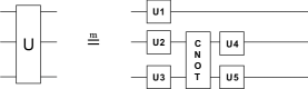
Figure 1: Unitaries (above) and tensors products (below). The unitary U represents a $n=3$ qubit transformation, where U is a $2^{n}\times 2^{n}$ ($8\times 8$) matrix. The unitary is implemented (equivalent or approximated) by the circuit on the right hand side. The single qubit unitaries are $2\times 2$ matrices, while CNOT is a $2^{2}\times 2^{2}$ matrix. The computation performed by the circuit is $(U3\otimes U4\otimes U5)(I2\otimes CNOT)(U1\otimes U2\otimes U3)$, where I2 is the identity $2\times 2$ matrix and $\otimes$ is the tensor product operator. The right hand side shows the tensor product of $2\times 2$ matrices.

n  m	0	1	2	3	4
2	1	2	3	-	-
3	3	9	14	20	-
4	8	22	54	73	100

Table 1: Upper bound on CNOT gate count when synthesizing a $m$ qubit circuit into $n$ qubits, with $m\leq n$. Data is presented by  [25]. The counts for $n=m$ are introduced by  [50]. The counts for state preparation ($m=0$) on two and three qubits are presented by  [59], and the count for state preparation on four qubits is introduced by [25]. The generalization and upper bound of is derived by [25]. Note that the CNOT counts grow very fast. For example, the upper bound on any unitary on 10 qubits is about about 500,000 CNOT gates.

2.1.1 Reasoning About Circuits and Algorithm Equivalence

A quantum transformation can be implemented by multiple distinct quantum circuits. that is when reasoning in terms of unitaries, there exist multiple decompositions of the unitary into terms that represent gates. Furthermore, when running on hardware, the unitary executed is often subtly different from the intended unitary.

Thus, it is often the case where we want to perform a particular quantum operation $A$ and because of external constraints we end up performing an approximation $B$, where $B\neq A$. Deciding which algorithm has executed is often referred to as distinguishability and several metrics with operational motivation have been proposed. Trace distance and fidelity [16, 9, 42] have been proposed for distinguishing states. Metrics such as the diamond norm [29] have been introduced to distinguish processes (algorithms).

Synthesis algorithms use norms to assess the solution quality, and their goal is to minimize $\norm{U-U_{S}}$, where $U$ is the unitary that describes the transformation and $U_{S}$ is the computed solution. They choose an error threshold $\epsilon$ and use it for convergence, $\norm{U-U_{S}}\leq\epsilon$. Early synthesis algorithms use the diamond norm, while more recent efforts [28, 31] use the Hilbert-Schmidt inner product between the conjugate transpose of $U$ and $U_{s}$. This is motivated by its lower computational overhead.

$$\langle U,U_{s}\rangle_{HS}=\Tr(U^{{\dagger}}U_{s})$$ (3)

2.2 Quantum Processors

Depending on the qubit technology, quantum processors may support different native gate sets, and qubits may connected in different topologies. We target processors with superconducting qubits since they implement a variety of topologies [52, 24, 49, 27] and are easier available. Most offer a native gate set consisting of rotations and CNOT gates {$R_{x}(90),R_{z}(\theta),CNOT$}. We believe that our results are easily generalized across superconducting qubit architectures which tend to support rotations and a single two qubit gate (CNOT , CRZ or SWAP).

While topology is important for superconducting qubits, implementations using trapped ion [12] qubits provide all-to-all connectivity through Mølmer-Sørensen [53] gates.

3 Synthesis Algorithm

Our goal is to design an algorithm that addresses currently perceived shortcomings of synthesis and that can be easily extended to new hardware in order to enable design space exploration in quantum programming. To be useful during the NISQ device era we use CNOT count as our primary optimality criteria. The synthesis algorithm described in the rest of this section combines a generalized space of parameterized circuits with an approximate A* search [22].

Intuitively, search based synthesis methods rely on the following approach. They start by “enumerating” the space of possible solutions. The construction of this space guarantees that if a solution exists, it will be contained in the enumeration. We rely on the same strategy. Then they start walking this space looking for solutions. Previous work uses “randomized” walk through genetic algorithms or Monte-Carlo methods. In contrast, we use a more regimented approach where we formulate the problem as a graph search and deploy established algorithms with good properties. In our case this is the A* algorithm. An example of the evolution of a search on a three qubit circuit is depicted in Figure 2.

3.1 Formulation of Synthesis as a Tree Search Problem

We first formulate the problem of synthesis as a graph search problem. We do this by constructing a tree of circuit structures.

The root node of our tree consists of $U3$ gates on every qubit line. For each node in the tree, there is one child for each possible CNOT position. For each CNOT position, we can construct the child by adding a CNOT in that position, and then adding two $U3$ gates on the qubit lines affected by the new CNOT.

For any circuit that can be constructed with a finite number of CNOT and $U3$ gates, our tree contains a node that can represent it. We will now provide constructive proof.

As a base case, the empty circuit, which contains 0 gates, implements the identity matrix, which can be represented by the root node with zero for all of its parameters, which also implements the identity. Now, assume that we can represent all circuits with up to $i$ gates. Given a circuit of length $i+1$, we can take the first $i$ gates, and find the node in our tree for it. For the last gate, if it is a CNOT , we can represent it by choosing the child of the node for the first $i$ gates that appends a CNOT in that position, and set the parameters of the two following $U3$ gates to 0. If the last gate is a $U3$, notice that the last gate on every qubit line in our circuit structure for any of our nodes is a $U3$ gate. The root node contains solely $U3$ gates, and any node further down the tree builds on the root node, so no qubit line is empty. The last gate on a qubit line is never a CNOT because we add $U3$ gates immediately after every CNOT . Therefore, the last $U3$ of the $i+1$ circuit is next to a $U3$ gate in the $i$ circuit, and we can combine these two $U3$ gates into a single $U3$ gate with different parameters, and we can use the same node in the tree. In any case, we have found a representation of the circuit of length $i+1$ in our tree.

The gate-set of $U3$ and CNOT is universal for quantum computing, meaning that any unitary matrix can be represented by a circuit consisting of only those gates. Since our tree contains a representation of any such circuit, our tree can represent a circuit that implements any given unitary. Furthermore, since our tree is organized such that circuits with fewer CNOT gates have a lower depth, if we find a lowest depth circuit that implements a given unitary, it will be a solution of lowest CNOT count. We have now reduced the problem of finding a circuit for a given unitary with the lowest CNOT count to a tree search problem, and then the numerical problem of finding values for the parameters. The first problem we can solve via A* search, and the second we can solve using numerical optimizer methods.

3.2 The Synthesis Algorithm

Our algorithm begins with a target unitary $U_{target}$, and a target gate-set. It also requires an acceptability threshold $\epsilon$, and a CNOT count limit $\delta$. The threshold provides the optimality metric for the solution. The CNOT count limit ensures termination and it is selected as depth bounds provided by other competing [25] methods: if we haven’t found a solution there are better methods available and we stop. The following description refers to the pseudocode in Algorithms 2 and 1.

The algorithm relies heavily on a successor function $s(n)$, which takes a node as input and returns a list of nodes, and an optimization function $p(n,U_{target})$, which takes a node and a unitary as input and returns a distance value. The function $H(d)$ is a heuristic function employed by A*, described in the next section.

The successor function, $s(n)$, is defined based on the target gate-set and topology. Given a node $n$ as input, $s(n)$generates a successor by appending to the circuit structure described by $n$. It appends a CNOT followed by two $U3$ gates. One successor is generated for each possible placement of the two-qubit gates allowed by the given topology. The one-qubit gates are placed immediately after the CNOT, on the qubit lines that the CNOT affects. A list of all successors generated from $n$ this way is returned. Note that CNOT and $U3$ can be replaced by different gates when using a different gate-set, as long as the gate-set remains universal and the single qubit gates are parameterizations of SU(2).

The optimization function, $p(n,U_{target})$, is used to find the closest matching circuit to a target unitary given a circuit structure. Given a node $n$ and a unitary $U_{target}$, let $U(n,\overline{x})$ represent the unitary implemented by the circuit structure represented by $n$ when using the vector $\overline{x}$ as parameters for the parameterized gates in the circuit structure. $D(U(n,\overline{x}),U_{target})$ is used as an objective function, and is given to a numerical optimizer, which finds $d={min}_{\overline{x}}D(U(n,\overline{x}),U_{target})$. The function $p(n,U_{target})$returns $d$.

The algorithm begins by generating the root node, which describes a circuit structure with one $U3$ gate on each qubit line. The distance value is found for the root node using $p(n,U_{target})$. These variables are initialized using the root node. The algorithm creates a priority queue that chooses the node $n$ that minimizes $f(n)$, and initializes the queue with the root node as the first entry. Now the algorithm enters a loop, in which it pops nodes from the queue. If no node remains in the queue, the algorithm exits with no solution. Otherwise, a node $n$ is successfully popped from the queue. Its successors $n_{1}$-$n_{k}$ are generated using $s(n)$. For each successor node $n_{i}$, the distance $d_{i}=p(n_{i})$ is calculated: this is a source of parallelism. If $d_{i}<\epsilon$, the current circuit $n_{i}$ is deemed acceptable and is returned. Otherwise, if the CNOT count of $n_{i}$ is within the limit $\delta$, the node $n_{i}$ is pushed onto the priority queue. If there is no acceptable solution with fewer than $\delta$ CNOT gates, eventually all possible structures with fewer gates will be tried, the queue will empty, and no solution will be returned.

The node that is returned from the algorithm, $n_{final}$, represents a circuit structure that includes a circuit that implements $U_{target}$to a distance within $\epsilon$. To find the specific circuit, the same numerical optimizer can be used, but this time to find $\overline{x}_{m}={arg\,min}_{\overline{x}}D(U(n,\overline{x}),U_{target})$. In practice, it is not necessary to re-run the optimizer since optimizer functions generally return both the minimum value and the values of the parameters that minimize it. The pair of $n_{final}$ and $\overline{x}_{m}$ constitute a complete description of a quantum circuit, and can be directly converted to quantum assembly.

(A)

(B) Figure 2: (A) Basic circuit block used for expanding the solution. We generate all alternatives where this structure is placed on linked qubit pairs. Each step adds six additional parameters to the optimization problem. (B) Example evolution of the search algorithm for a three qubit circuit. We start by placing a layer of single qubit gates, then generate the next two possible solutions. Each is evaluated and in this case the upper circuit is closer to the target unitary, leading to a smaller heuristic value. Since this circuit This circuit is then expanded with its possible two successors. These are again instantiated by the optimizer. The second circuit from the top has an acceptable distance and is reported as the solution. The path in red shows the evolution of the solution. The solutions enclosed by the dotted line have been evaluated during the search.

Algorithm 1 Helper Functions

1:function s($n$) return $\{n+\textsc{CNOT\ }+U3\otimes U3\text{for all possible {CNOT\ }positions}\}$

2:end function

3:

4:function p($n$, $U$) return ${min}_{\overline{x}}D(U(n,\overline{x}),U)$

5:end function

6:

7:function h($d$)

8:return $d*a$ $\triangleright$ $a$ is a constant determined via experiment. See section 3.3.1

9:end function

Algorithm 2 Search Synthesis

1:function synthesize($U_{target}$, $\epsilon$, $\delta$)

2:     $n\leftarrow\text{representation of $U3$ on each qubit}$

3:     push $n$ onto $queue$ with priority h($d_{best}$)$+0$

4:     while $queue$ is not empty do

5:         $n\leftarrow\textbf{pop from }queue$

6:         for all $n_{i}\in$s($n$) do

7:              $d_{i}\leftarrow$ p($n_{i}$, $U_{target}$)

8:              if $d_{i}<\epsilon$ then

9:                  return $n_{i}$

10:              end if

11:              if CNOT count of $n_{i}<\delta$ then

12:                  push $n_{i}$ onto $queue$ with priority h($d_{i}$)$+$CNOT count of $n_{i}$

13:              end if

14:         end for

15:     end while

16:end function

3.3 A* Search Strategy

The A* algorithm has been developed for graph traversals and it attempts to find a path between a start and target node. At each step, a partial solution is expanded using a successor function, and the successors are added to a priority queue. Then a new partial solution is chosen from the queue that minimizes a cost function. The first path from start to finish is the final solution. Given a partial solution, the algorithm picks the next partial solution based on the cost of its already computed path and an estimate of the cost required to extend it all the way to the target. A* selects the successor node $n$ that minimizes $f(n)=g(n)+h(n)$ where

• $f(n)$ is the estimated total cost of the path from start to finish

• $g(n)$ is the cost of the path from the start to $n$

• $h(n)$ is a heuristic function that estimates the cost of the cheapest path from $n$ to the target

The algorithm terminates when it reaches the target node or if there are no paths eligible to be extended. The heuristic function is problem-specific and directly determines the time complexity of A*. If the heuristic function is admissible, meaning that it never overestimates the actual cost to get to the target, A* is guaranteed to return a least-cost path. A* can be run with an inadmissible heuristic to obtain sub-optimal solutions with a faster runtime than it would take to obtain guaranteed optimal solutions.

For synthesis, the selection of $g(n)$ is obvious as the CNOT count of the partial solution $n$. The challenge was to determine the heuristic function $h(n)$. After several attempts at deriving it from first principles we have opted for a data-driven approach described below.

3.3.1 Heuristic Function Tuning

We first use breadth first search for synthesis. We ran breadth first search on each of our three-qubit benchmarks, and examined the details of the search along the final paths. At each partial solution along the path, we recorded the distance value at that step to the remaining number of CNOT gates (calculated by subtracting the current number of CNOT ’s at that step to the final value reach in that run of the program). We then fit the data, and found a best fit line with slope $a=9.3623$.

The fit gives us the heuristic function $h(n)=D(U(n,\overline{x}_{m}),U_{target})*9.3623$, or $h(n)=p(n,U_{target})*9.3623$. Although the fit was not very well correlated ($r^{2}=0.4102$), we found experimentally that the heuristic yielded excellent results. Running the same set of benchmarks with the A* heuristic, we found that the same quality solutions were found, but runtime was significantly faster. For example, brute force search for three qubit QFT takes one hour, while A* takes only seven minutes.

3.4 Unitary Distance Metric

We use the following distance function based on the Hilbert-Schmidt inner product. If N is the dimension of the unitaries,

$$D(U,U_{target})=1-\frac{\langle U,U_{target}\rangle_{HS}}{N}=1-\frac{\Tr(U^{{\dagger}}U_{target})}{N}\\$$ (4)

The formula is based on the fact that the inverse of a unitary matrix is its conjugate transpose. If the synthesis succeeds and $U$ is not distinguishable from $U_{target}$, the product $U^{{\dagger}}U_{target}=I_{N}$, where $I$ is the identity matrix. Furthermore, the maximum magnitude that the trace of a unitary matrix can have is its size N, which occurs at the identity (up to a phase). The closer $U^{{\dagger}}U_{target}$ is to identity, the closer $\frac{\Tr(U^{{\dagger}}U_{target})}{N}$ is to $N$, thus the closer our distance function is to $0$.

Note that variations of formulas using Hilbert-Schmidt inner product have been previously used in synthesis algorithms [28, 34], and ours has the following properties

• The distance is 0 when compilation is exact.

• It is easy to compute.

• It has operational meaning.

4 Experimental Setup

Software Implementation: We implemented our algorithm in python 3.7.4, using numpy 1.14.4 for performing matrix multiplication, and the COBYLA numerical optimizer provided with scipy 1.2.0. We use multiprocessing.Pool for parallelism. Most of the tests ran on a single node of the Cori supercomputer hosted at the National Energy Research Scientific Computing Center (NERSC), where nodes contain two Intel Xeon E5-2698 v3 ("Haswell") processors at 2.3 GHz (32 cores total).

The implementation returns a circuit when it finds a solution with a Hilbert-Schmidt distance value less than $10^{-10}$ from the target. This is enough that the resulting circuit is not distinguishable from the original, as well as avoiding numerical errors within the software stack.

Benchmarks: We concentrate on algorithms spanning a small number of qubits as we are interested in compiling for the Noisy Intermediate-Scale Quantum devices. Our goal is to demonstrate the value of synthesis to practitioners under several usage scenarios: 1) compiling unitaries; 2) gate set design exploration; and 3) circuit optimization.

The benchmark suite is composed of “traditional” algorithms used by other evaluation studies [39], and it contains the Quantum Fourier Transform [41] algorithm, HHL [21], Variational Quantum Eigensolver [36] algorithm, together with important quantum kernels such as Toffoli gates. In addition to qubit based circuits we consider the qutrit circuits described in [7].

Experimental Results: A summary of the results is presented in Table 3. The columns labeled CNOT show our implementation, annotated with the topology of the target chip. Besides circuit depth, we present the Hilbert-Schmidt distance of the solution and total compilation time.

Customizing for QPU Gate Set and Topology: We target directly the gate set native to the quantum processor. Our initial implementation was tailored for the QNL8QR-v5 processor which supports in hardware the $R_{x}(90),R_{z}{\theta},CNOT$ gates and its qubits are connected in a line topology. We have also re-targeted the algorithm for the IBM Q 5 qubit chip, with a similar native gate set but a bow-tie/triangle topology.

Use Cases: To showcase the extensibility of the proposed approach we consider synthesis of qutrit gates, a problem of interest to hardware and algorithm designers. To showcase the interaction between synthesis and the rest of the software development stack (optimizing compilers and mappers) we examine using synthesis during the circuit optimization phase. In addition, we are interested determining the impact of specializing the synthesis algorithm for a different topology. For this we report the length of the synthesized circuits after being compiled and optimized using QISKit. For example. the “CNOT+QISKit” label describes the experiment where we compile our generated circuit with QISKit.

Comparison with State-of-the-Art: In Table 3, the column labeled UQ shows the number of CNOT generated by the UniversalQ [26] compiler, a state-of-the-art synthesis tool that uses internally multiple linear algebra based decomposition methods, including Cosine-Sine. For UQ, we report the best result obtained by any decomposition method available.

5 Compiling Unitaries to Circuits

In all cases illustrated in Table 3 we were able to synthesize circuits shorter than the theoretical upper bounds provided by  [25]. Their CNOT count upper bounds for Q=2 and Q=3 are 3 and 20 respectively. When comparing against the UniversalQ compiler, we generate significantly shorter circuits, using on average $2.4\times$ fewer CNOTs, and as high as $5.3\times$.

Comparisons against other techniques are harder, due to lack of availability of software implementations (some not released, some described only in algorithmic form) and differences in native gate sets. When comparing against [34], they report no compilations shorter than eight two-qubit gates (Mølmer-Sørensen) for a sample of 3-qubit random unitaries. Shortest circuit obtained by our tool has 3 CNOT gates. Amy et al [6] report eight CNOT gates for Toffoli, while our implementation finds a circuit with only six CNOTs. They also report not being able to synthesize three qubit QFT using less than 10 CNOT gates.

At small qubit count, perhaps the most important comparison is against the depth obtained by hand optimization. From this perspective our algorithm behaves well. For example, the optimal CNOT count for Toffoli [51] is six, which our algorithm matches. When mapping to a linear topology, implementations introduce extra SWAPs, up to a total of 12 CNOT gates. Our linear topology Toffoli contains only eight CNOTs. The Fredkin gate is usually implemented as Toffoli sandwiched between two more CNOT gates. Hand optimized Fredkin for linear topologies is available in Cirq [1] with nine CNOTs, while our implementation uses only eight. On a well connected IBM topology we synthesize a Fredkin using only seven CNOTs: IBM QISKit will produce a circuit with eight CNOTs.

The HHL implementation was obtained from the QNL8QR-v5 development team. Mapped to a linear topology by hand, the circuit had seven CNOT gates, while our implementation contains only three.

For QFT, the best known implementations use two and six CNOTs, for two and three qubit circuits respectively, assuming a well connected topology. In our case, we obtain circuits that are three and seven long, respectively. After examining the resulting circuits, omitted for brevity, we attribute the difference to limitations in the numerical optimizer (COBYLA in this case). In the optimal circuit, there are places where there are no single qubit gates between CNOT gates. It seems that all numerical optimizers we have experimented with have trouble zeroing these gates, thus leading to a slightly longer circuit. Note that we do obtain good results for QFT on a line topology: best circuits have nine CNOTs, while ours has eight.

5.1 Impact of Topology

Embedding the circuit topology within the synthesis algorithm matters, perhaps even more than developing an optimal algorithm for well connected topologies.

The first observation is that existing algorithms report large ($4\times$) proportionality constants when specializing for a restricted topology. In our case we observe only modest increases, up to 15% for the workload and for only five of the tested circuits. In some cases, we obtain circuits shorter than previously known. This indicates that we can handle well restricted topologies.

Even more important is the empirical observation that the rest of the compilation toolkit (circuit optimizers + mappers) can only increase (never decrease) the depth of our synthesized circuits. This is illustrated in Table 3 by the columns with the label “QISKit”. In the first experiment, we take the circuits synthesized for a linear topology and compile them with QISKit for the better connected bowtie topology. We enable the highest level of optimization available. The circuits optimized and mapped by QISKit have the same length as the input circuits. In the second experiment, data presented in the Table, we compile the circuits synthesized for the bowtie with QISKit configured for a linear topology. In this case we observe a 53% average increase in CNOT count, with values as high as $4\times$.

To us, this indicates that if the goal for NISQ devices is obtaining optimally short circuits, techniques like our are more likely to deliver consistently than traditional optimizers and mappers.

5.2 Synthesis and Circuit Optimization

The three qubit circuit “EntangledX” provides an illustration of the benefits of synthesis embedded in the circuit optimization workflow. The gate is a building block for a VQE implementation using the [[4,2,2]] error detection code [19] and it is parameterized by a rotation angle. The authors run the circuit sampling the parameter for robust behavior, the sampling is directed by the results of the previous run.

The (painstakingly) hand optimized and most generic version contains four CNOT gates, which we match for most values of the rotation angle. However, for some angles, we were able to achieve circuits with only two or three CNOT gates.

		CNOT count			Mapped by QISKit on linear topology			Unitary distance		Compile time (s)
ALG	Qubits	CNOT	CNOT	UQ	$CNOT$ + QISKit	$CNOT$ + QISKit	UQ+QISKit	$||CNOT||$	$||CNOT||$	T($CNOT$)	T($CNOT$)	T(UQ)
QFT	2	3	3	3	3	3	3	$2.08*10^{-15}$	$3.86*10^{-15}$	3	3	<1
QFT	3	8	7	15	8	13	27	$1.56*10^{-14}$	$8.66*10^{-15}$	610	341	<1
Fredkin	3	8	7	9	8	16	26	$2.22*10^{-15}$	$4.69*10^{-15}$	493	849	<1
Toffoli	3	8	6	9	8	12	21	$1.10*10^{-14}$	$1.88*10^{-14}$	714	1015	<1
Peres	3	7	6	19	7	9	47	$1.01*10^{-14}$	$8.25*10^{-15}$	331	285	<1
HHL	3	3	3	16	3	3	21	$2.46*10^{-14}$	$1.44*10^{-16}$	12	12	<1
Or	3	8	6	10	8	9	19	$4.01*10^{-14}$	$8.65*10^{-15}$	492	340	<1
EntangledX	3	4	4	9	4	16	21	$7.77*10^{-17}$	$2.11*10^{-16}$	27	60	<1
QFT	4	14		89			DNR	$1.41*10^{-12}$		410250		<1

Figure 3: Summary of synthesis results for several algorithms and unitaries. Q = number of qubits. The topology used during synthesis is denoted in the caption. Theoretical CNOT count upper bounds for Q=2 and Q=3 are 3 and 20 respectively.

5.3 Retargeting to Qutrits

Qutrits extend qubits to systems with three logical values 0, 1 and 2. They are represented by unitaries from SU(3) and extend from binary to ternary logic to explore a space with $3^{n}$ dimensions. There exist several [58, 10] decompositions and parameterizations, all using eight independent parameters. Gates to implement qutrit operations have been explored only recently [7] for qubit based systems, mostly motivated by the need [33] for modeling physical phenomena.

For our study, we implement a CSUM two-qutrit gate, which adds the value of the first qutrit to the second qutrit $CSUM(\ket{11})=\ket{12}$. Our synthesis matches the hand optimized implementation by [7]. For brevity, we omit detailed results.

5.4 Acceptability Threshold Tuning

Our algorithm terminates upon finding a circuit with a distance value within an acceptability threshold $\epsilon$. Its value is determined by two requirements: 1) the implementation should be able to meet it in terms of numerical accuracy; and 2) the resulting unitary should be indistinguishable from the original.

For the first criteria we tried synthesizing four of our benchmarks threshold limits at powers of ten ranging from $0.1$ to $10^{-12}$. We found that with only two exceptions, threshold limits in the range $0.01\leq\epsilon\leq 10^{-12}$ resulted in final solutions with distance on the order of $10^{-12}-10^{-14}$. The two exceptions were both 3-qubit QFT solutions, one with a solution on the order of $10^{-10}$ and one with $10^{-8}$. We concluded that a threshold of $10^{-10}$ will ensure we have the best quality answer our numerical optimizers will be able to give us.

To ensure this threshold is sufficient for real world applications, we ran another experiment to relate matrix distance to the KL divergence of probability distributions. We generated random unitaries that are close to the identity, multiplied these by fully random unitaries. For each pair of fully random unitary and product of random unitary and near-identity random unitary, we recorded the matrix distance and the KL divergence between the final probability distributions after measuring the result of applying the two unitaries to the same randomly generated state vector, recording the worst case KL divergence after trying 1000 random state vectors. The results showed a clear correlation between KL divergence and Hilbert-Schmidt distance, with the acceptability threshold of $10^{-10}$ yielding a maximum KL divergence of $2.56*10^{-9}$. Even for a looser threshold of $10^{-8}$, the maximum KL divergence was $5.20*10^{-8}$, so the threshold might even be loosened in practice.

5.5 Solution Quality

The Hilbert-Schmidt distance between our solution and the original unitary is presented in Table 3. The values range from $10^{-14}$ to $10^{-17}$. We tested the resulting circuits on 1,000 random input state vectors: the results are indistinguishable from the original circuit.

We only report the total number of CNOT gates in the generated circuit. The upper bound on the total number of gates in a $Q$ qubits circuit is given by $Q+5*CNOT$. This includes single qubit gates and is based on the fact that each $U_{3}$ gate is expanded into at most four  single qubit rotations.

5.6 Running Time

The running time of our algorithm is presented in Table 3. In the current implementation the algorithm performance is determined mainly by the performance of the numerical optimizer. We have experimented with several Python interoperable implementations: CMA-ES [20], COBYLA and BOBYQA. We have selected COBYLA as the default optimizer. Given a circuit with $Q$ qubits and depth $d$, the total number of parameters is $Num\_Params=3*Q+6*d$. For reference, typical durations for depth six circuits are $\approx 130s$, $\approx 210s$ at depth eight and $\approx 620s$ at depth 14.

Our implementation is otherwise very well optimized. Some techniques are Python specific, some are generally applicable. We used our own object-based representation of quantum gates which allowed us a simple and memory-efficient way of implementing the successor function. These objects create and multiply together numpy matrices and we have thoroughly optimized the code to minimize object copies. We also added a circuit-optimization step which rearranges our circuit component graph to perform matrix products with the minimum number of operations. The gate parametrization is minimized by replacing the parameterized single qubit gate after the control line of a CNOT gate with a simpler parameterization with only two parameters (because a parameterized Z gate can commute through the control line of a CNOT and can be absorbed by the parameterized gate on the other side). The vast majority of our runtime is spent in creating matrices from circuit component graphs within the objective function calls of the optimizer, so we have focused our optimization efforts on tuning the optimizer to make fewer objective function calls and improving our matrix generation to be more efficient. We also used beam searching, popping multiple nodes off the top of the queue at a time, in order to take better advantage of parallelism. Beam searching lets us evaluate nodes that we would have to backtrack to in parallel rather than sequentially. In the case of approximate A*, it can lead to a different solution, but it will only find one at least as good (in terms of minimizing CNOT count) as it would have found otherwise.

Note that some of the runtime overhead cannot be avoided in a Python code base, but disappears when re-implementing in a performance oriented language such as C/C++. We have chosen Python for the easy interoperability with all available [2, 1, 45] quantum compilation infrastructures.

6 Discussion

Overall, we believe our results are very encouraging and show the general applicability of quantum circuit synthesis techniques during the NISQ decade(s). Looking back, the field has progressed steadily. Solovay and Kitaev open the field by showing that a solution exists when using any universal gate set. Later efforts show that solutions exist when restricting the gate sets to “almost native”. The emphasis then moved on to improving quality (depth) of the solution, and the field has steadily progressed from computing huge  to computing decent solutions.

We have shown concrete results where we match the shortest known depth for several algorithms, we have shown results where we reduce depth for constrained topologies (line) and we have shown the retargetability of the implementation to new gate sets. Equally important, we have shown empirical evidence that traditional optimization techniques (peephole optimizers and mappers) are unlikely to match the quality of the circuits generated by synthesis. We believe that the results alleviate some of the doubts faced by synthesis approaches: generated circuits are too deep and there is no topology awareness.

Due to its potential, we believe a roadmap for synthesis targeting NISQ devices is worth developing. Our study illustrates some of the solutions, as well as the associated open problems. For practical purposes, quality of the solution is important (short depth), followed by scalability. Given that we have shown optimality and topology awareness, for the near future, scalability at small qubit scale is worth exploring as it will lead to establishing robust building blocks when considering scalability with qubits.

Synthesis for early NISQ (small) circuits: There are several orthogonal directions to pursue to improve speed:

• Better numerical optimizers. The judicious choice of the numerical optimizer is probably the most important factor.  [46] provide a very useful overview of derivative-free methods. Based on their recommendations, the first step is to select the best known derivative-free methods such as TOMLAB/MULTIMIN, TOMLAB/GLCCLUSTER, MCS or TOMLAB/LGO. The second step is to employ meta-optimization techniques that combine different approaches. Note that in our case the choice was limited due to lack of availability of open source Python or C based implementations. It is also worth considering building ad-hoc optimizers for synthesis based on tensor networks and gradient descent. These have the advantage of high GPU performance.

• Better parallelization of the search algorithm. There are two levels of parallelism within numerical optimization based algorithms. At the inner level, the first challenge is that the numerical optimizer itself needs to have a good parallel implementation.This does not seem to be the case with the publicly available implementations which exploit it only in small matrix BLAS function calls. There is an outer level of embarrassing parallelism across optimizer invocations, given by the evaluation of the partial solutions at a given search step. This is proportional with the number of qubits in the algorithm. Since in our case the optimizer performs best single threaded, shared memory parallelism is sufficient. Implementations will eventually need to move to distributed memory parallelism, given the availability of parallel numerical optimizers.

  Synthesis for late NISQ (large) circuits: For circuits with tens of qubits memory and computational requirements for synthesis may be prohibitive, as unitaries scale exponentially with $2^{q}$. Given an already existing circuit, a straightforward way to incorporate synthesis is to partition it in manageable size blocks, optimize these individually and recombine. For algorithm discovery, synthesis will have to be incorporated into generative models for domain science. For example, frameworks such as OpenFermion can already generate arbitrary size circuits. We have already started exploring these directions using the current algorithm.

  7 Related Work

  A fundamental result, which spurred the apparition of quantum circuit synthesis is provided by the Solovay Kitaev (SK) theorem.The theorem relates circuit depth to the quality of the approximation and its proof is by construction  [13, 40, 4]. Different approaches [13, 14, 8, 6, 35, 17, 11, 57, 38, 5, 48] to synthesis have been introduced since, with the goal of generating shorter depth circuits. These can be coarsely classified based on several criteria: 1) target gate set; 2) algorithmic approach; and 3) solution distinguishability.

  Target Gate Set: The SK algorithm is quite general in the sense that it is applicable to any universal gate set. Synthesis can be improved in terms of both speed and optimality by specializing the gate set. Examples include synthesis of z-rotation unitaries with Clifford+V approximation [47] or Clifford+T gates [30]. When ancillary qubits are allowed, one can synthesize a single qubit unitaries with the Clifford+T gate set [30, 3, 43]. While these efforts propelled the field of synthesis, they are not used on NISQ devices, which offer a different gate set ($R_{x},R_{z},CNOT$ and Mølmer-Sørensen all-to-all). Several [25, 50, 34] other algorithms, discussed below have since emerged.

  Algorithmic Approaches: The earlier attempts inspired by Solovay Kitaev use a recursive (or divide-an-conquer) formulation, sometimes supplemented with search heuristics at the bottom. More recent search based approaches are illustrated by the Meet-in-the-Middle [6] algorithm.

  Several approaches use techniques from linear algebra for unitary/tensor decomposition. [11] use QR matrix factorization via Given’s rotation and Householder transformation  [57], but there are open questions as to the suitability for hardware implementation because these algorithms are expressed in terms of row and column updates of a matrix rather than in terms of qubits.

  The state-of-the-art upper bounds on circuit depth are provided by techniques [50, 25] that use Cosine-Sine decomposition. The Cosine-Sine decomposition was first used by [55] for compilation purposes. In practice, commercial compilers ubiquitously deploy only KAK [56] decompositions for two qubit unitaries.

  The basic formulation of these techniques is topology independent. Specializing for topology increases the upper bound by rather large constants,  [50] mention a factor of nine, improved by [25] to $4\times$. The published approaches are hard to extend to different qubit gate sets and it remains to be seen if they can handle qutrits. Furthermore, it seems that the numerical techniques [54] required for CSD still require refinements as they cannot handle numerically challenging cases.

  Several techniques use numerical optimization, much as we did. They describe the gates in their variational/continuous representation and use optimizers and search to find a gate decomposition and instantiation. The work closest to ours is by [34] which use numerical optimization and brute force search to synthesize circuits for a processor using trapped ion qubits. Their main advantage is the existence of all-to-all Mølmer-Sørensen gates, which allow a topology independent approach. The main difference between our work and theirs is that they use randomization and genetic algorithms to search the solution space, while we show a more regimented way. When Martinez et al. describe their results, they claim that Mølmer-Sørensen counts are directly comparable to CNOT counts. By this metric, we seem to generate comparable or shorter circuits than theirs. It is not clear how their approach behaves when topology constraints are present. The direct comparison is further limited due to the fact that they consider only randomly generated unitaries, rather than algorithms or well understood gates such as Toffoli or Fredkin.

  Another topology independent numerical optimization technique is presented by [28]. In this case, the main contribution is to use a quantum annealer to do searches over sequences of increasing gate depth. They report results only for two qubit circuits.

  All existing studies focus on the quality of the solution, rather than synthesis speed. They also report results for low qubit concurrency: Khatri et al. [28] for two qubit systems, Martinez et al. [34] for systems up to four qubits.

  Solution Distinguishability: Synthesis algorithms are classified as exact or approximate based on distinguishability. This is a subtle classification criteria, as most algorithms can be viewed as either. For example, [6] proposed a divide-and-conquer algorithm called Meet-in-the-Middle (MIM). Designed for exact circuit synthesis, the algorithm may also be used to construct an $\epsilon$-approximate circuit. The results seem to indicate that the algorithm failed to synthesize a three qubit QFT circuit.

  Furthermore, on NISQ devices, the target gate set of the algorithm (e.g. T gate) may be itself implemented as an approximation when using native gates.

  We classify our approach as approximate since we accept solutions at a small distance from the original unitary. In a sense, when algorithms move from design to implementation, all algorithms are approximate due to numerical floating point errors.

  8 Conclusion

  In this work we have shown methods to compile arbitrary quantum unitaries into a sequence of gates native to several superconducting qubit based architectures. The algorithm we develop is topology aware and it is easily re-targeted to new gates sets or topologies. Results indicate that we can match, or even improve on when topology is restricted, the shortest depth circuit implementation published for several widely used algorithms and gates. We also show empirical evidence which supports an important conjecture: the benefits of incorporating topology directly into synthesis cannot be replicated if relying on all-to-all synthesis and traditional (peephole base) optimizing quantum compilers or mappers.

  The method is slow but it does produce good results in practice. For the early NISQ era, which is likely to be characterized by hero experiments, the overhead seems acceptable. Even when superseded by faster algorithms, we believe our results provide a good quality measure threshold for these implementations.

  Looking forward, better numerical optimizers are required for enhancing the palatability of quantum circuit synthesis. These will alleviate some of the need for developing better search algorithms.

References

- [1] Google cirq. Available at https://github.com/quantumlib/Cirq.
- [2] Ibm qiskit. Available at https://qiskit.org/.
- [3] Classical and Quantum Computation. American Mathematical Society, Boston, MA, 2012.
- [4] O. Al-Ta’Ani. Quantum Circuit Synthesis using Solovay-Kitaev Algorithm and Optimization Techniques. PhD thesis, 2015.
- [5] M. Amy and M. Mosca. T-count optimization and Reed-Muller codes. arXiv:1601.07363v1, 2016.
- [6] Matthew Amy, Dmitri Maslov, Michele Mosca, and Martin Roetteler. A meet-in-the-middle algorithm for fast synthesis of depth-optimal quantum circuits. Trans. Comp.-Aided Des. Integ. Cir. Sys., 32(6):818–830, June 2013.
- [7] M Blok, V Ramasesh, J Colless, K O’Brien, T Schuster, N Yao, and I Siddiqi. Implementation and applications of two qutrit gates in superconducting transmon qubits. Bulletin of the American Physical Society 2018, 2018.
- [8] Alex Bocharov and Krysta M. Svore. Resource-optimal single-qubit quantum circuits. Phys. Rev. Lett., 109:190501, Nov 2012.
- [9] Heinz-Peter Breuer, Elsi-Mari Laine, and Jyrki Piilo. Measure for the Degree of Non-Markovian Behavior of Quantum Processes in Open Systems. Physical Review Letters, 103:210401, Nov 2009.
- [10] J. B. Bronzan. Parametrization of su(3). Phys. Rev. D, 38:1994–1999, Sep 1988.
- [11] S. S. Bullock and I. L. Markov. An arbitrary two-qubit computation in 23 elementary gates or less. In Proceedings 2003. Design Automation Conference (IEEE Cat. No.03CH37451), pages 324–329, June 2003.
- [12] J. I. Cirac and P. Zoller. Quantum computations with cold trapped ions. Phys. Rev. Lett., 74:4091–4094, May 1995.
- [13] C. M. Dawson and M. A. Nielson. The Solovay-Kitaev Algorithm. Quant. Info. Comput., 6(1):81–95, 2005.
- [14] A. De Vos and S. De Baerdemacker. Block- synthesis of an arbitrary quantum circuit. Phys. Rev. A, 94:052317, Nov 2016.
- [15] D Deutsch. Quantum computational networks. 425:73–90, 09 1989.
- [16] Alexei Gilchrist, Nathan K. Langford, and Michael A. Nielsen. Distance measures to compare real and ideal quantum processes. Phys. Rev. A, 71:062310, Jun 2005.
- [17] B. Giles and P. Selinger. Exact synthesis of multiqubit Clifford+T circuits. Physical Review Letters., 87(3):032332, March 2013.
- [18] Brett Giles and Peter Selinger. Exact synthesis of multiqubit clifford+ circuits. Phys. Rev. A, 87:032332, Mar 2013.
- [19] M. Grassl, Th. Beth, and T. Pellizzari. Codes for the quantum erasure channel. Phys. Rev. A, 56:33–38, Jul 1997.
- [20] Nikolaus Hansen. The CMA evolution strategy: A tutorial. CoRR, abs/1604.00772, 2016.
- [21] A. W. Harrow, A. Hassidim, and S. Lloyd. Quantum Algorithm for Linear Systems of Equations. Physical Review Letters, 103(15):150502, October 2009.
- [22] P. E. Hart, N. J. Nilsson, and B. Raphael. A formal basis for the heuristic determination of minimum cost paths. IEEE Transactions on Systems Science and Cybernetics, 4(2):100–107, July 1968.
- [23] Jeremy Hsu. Ces 2018: Intel’s 49-qubit chip shoots for quantum supremacy. https://spectrum.ieee.org/tech-talk/computing/hardware/intels-49qubit-chip-aims-for-quantum-supremacy, 2018.
- [24] IBM. Ibm q 5 yorktown chip. https://www.research.ibm.com/ibm-q/technology/devices/#ibmqx2, 2019.
- [25] Raban Iten, Roger Colbeck, Ivan Kukuljan, Jonathan Home, and Matthias Christandl. Quantum circuits for isometries. Physical Review A, 93:032318, Mar 2016.
- [26] Raban Iten, Oliver Reardon-Smith, Luca Mondada, Ethan Redmond, Ravjot Singh Kohli, and Roger Colbeck. Introduction to UniversalQCompiler. arXiv e-prints, page arXiv:1904.01072, Apr 2019.
- [27] Julian Kelly. A preview of bristlecone, google’s new quantum processor. https://research.googleblog.com/2018/03/a-preview-of-bristlecone-googles-new.html, 2018.
- [28] Sumeet Khatri, Ryan LaRose, Alexander Poremba, Lukasz Cincio, Andrew T. Sornborger, and Patrick J. Coles. Quantum-assisted quantum compiling. arXiv e-prints, page arXiv:1807.00800, Jul 2018.
- [29] A. Yu. Kitaev, A. H. Shen, and M. N. Vyalyi. Classical and Quantum Computation. American Mathematical Society, Boston, MA, USA, 2002.
- [30] V. Kliuchnikov, D. Maslov, and M. Mosca. Practical approximation of single-qubit unitaries by single-qubit quantum clifford and t circuits. IEEE Transactions on Computers, 65(1):161–172, Jan 2016.
- [31] Vadym Kliuchnikov, Alex Bocharov, and Krysta M. Svore. Asymptotically Optimal Topological Quantum Compiling. Physical Review Letters, 112:140504, Apr 2014.
- [32] Vadym Kliuchnikov, Dmitri Maslov, and Michele Mosca. Fast and efficient exact synthesis of single-qubit unitaries generated by clifford and t gates. Quantum Info. Comput., 13(7-8):607–630, July 2013.
- [33] K. A. Landsman, C. Figgatt, T. Schuster, N. M. Linke, B. Yoshida, N. Y. Yao, and C. Monroe. Verified quantum information scrambling. Nature, 567(7746):61–65, 2019.
- [34] E. Martinez, T. Monz, D. Nigg, P. Schindler, and R. Blatt. Compiling quantum algorithms for architectures with multi-qubit gates. ArXiv e-prints, July 2016.
- [35] Esteban A Martinez, Thomas Monz, Daniel Nigg, Philipp Schindler, and Rainer Blatt. Compiling quantum algorithms for architectures with multi-qubit gates. New Journal of Physics, 18(6):063029, 2016.
- [36] Jarrod R McClean, Jonathan Romero, Ryan Babbush, and Alán Aspuru-Guzik. The theory of variational hybrid quantum-classical algorithms. New Journal of Physics, 18(2):23023, 2016.
- [37] Samuel K. Moore. Ibm edges closer to quantum supremacy with 50-qubit processor. https://spectrum.ieee.org/tech-talk/computing/hardware/ibm-edges-closer-to-quantum-supremacy-with-50qubit-processor, 2017.
- [38] Mikko Möttönen, Juha J. Vartiainen, Ville Bergholm, and Martti M. Salomaa. Quantum circuits for general multiqubit gates. Phys. Rev. Lett., 93:130502, Sep 2004.
- [39] Prakash Murali, Jonathan M. Baker, Ali Javadi Abhari, Frederic T. Chong, and Margaret Martonosi. Noise-Adaptive Compiler Mappings for Noisy Intermediate-Scale Quantum Computers. arXiv e-prints, page arXiv:1901.11054, Jan 2019.
- [40] A. B. Nagy. On an implementation of the Solovay-Kitaev algorithm. arXiv:quant-ph/0606077, 2016.
- [41] VICTOR NAMIAS. The Fractional Order Fourier Transform and its Application to Quantum Mechanics. IMA Journal of Applied Mathematics, 25(3):241–265, 03 1980.
- [42] Michael A. Nielsen and Isaac L. Chuang. Frontmatter, pages i–viii. Cambridge University Press, 2010.
- [43] Adam Paetznick and Krysta M. Svore. Repeat-until-success: Non-deterministic decomposition of single-qubit unitaries. Quantum Info. Comput., 14(15-16):1277–1301, November 2014.
- [44] M. J. D. Powell. A Direct Search Optimization Method That Models the Objective and Constraint Functions by Linear Interpolation, pages 51–67. Springer Netherlands, Dordrecht, 1994.
- [45] Rigetti. Forest and pyquil documentation. http://docs.rigetti.com/en/stable/.
- [46] Luis Miguel Rios and Nikolaos V. Sahinidis. Derivative-free optimization: a review of algorithms and comparison of software implementations. Journal of Global Optimization, 56(3):1247–1293, Jul 2013.
- [47] Neil J. Ross. Optimal ancilla-free clifford+v approximation of z-rotations. Quantum Info. Comput., 15(11-12):932–950, September 2015.
- [48] G. Seroussi and A. Lempel. Factorization of symmetric matrices and trace-orthogonal bases in finite fields. SIAM Journal on Computing, 9(4):758–767, 1980.
- [49] E. A. Sete, W. J. Zeng, and C. T. Rigetti. A functional architecture for scalable quantum computing. In 2016 IEEE International Conference on Rebooting Computing (ICRC), pages 1–6, Oct 2016.
- [50] V. V. Shende, S. S. Bullock, and I. L. Markov. Synthesis of quantum-logic circuits. IEEE Transactions on Computer-Aided Design of Integrated Circuits and Systems, 25(6):1000–1010, June 2006.
- [51] Vivek V. Shende and Igor L. Markov. On the CNOT-cost of TOFFOLI gates. arXiv e-prints, page arXiv:0803.2316, Mar 2008.
- [52] Irfan Siddiqi. "quantum nanoelectronics laboratory, university of california at berkeley". http://qnl.berkeley.edu/, 2019.
- [53] Anders Sørensen and Klaus Mølmer. Entanglement and quantum computation with ions in thermal motion. Physical Review A, 62:022311, Aug 2000.
- [54] Brian D Sutton. Computing the complete cs decomposition. Numerical Algorithms, 50(1):33–65, 2009.
- [55] Robert R. Tucci. A Rudimentary Quantum Compiler(2cnd Ed.). arXiv e-prints, pages quant–ph/9902062, Feb 1999.
- [56] Robert R. Tucci. An Introduction to Cartan’s KAK Decomposition for QC Programmers. arXiv e-prints, pages quant–ph/0507171, Jul 2005.
- [57] J. Urias. Householder factorization of unitary matrices. J. Mathematical Physics, 51:072204, 2010.
- [58] Nikolay Vitanov. Synthesis of arbitrary su(3) transformations of atomic qutrits. Phys. Rev. A, 85, 03 2012.
- [59] Marko Znidaric, Olivier Giraud, and B Georgeot. Optimal number of controlled-not gates to generate a three-qubit state. Phys. Rev. A, 77, 03 2008.