Binarized Canonical Polyadic Decomposition for Knowledge Graph Completion

Abstract

Methods based on vector embeddings of knowledge graphs have been actively pursued as a promising approach to knowledge graph completion. However, embedding models generate storage-inefficient representations, particularly when the number of entities and relations, and the dimensionality of the real-valued embedding vectors are large. We present a binarized CANDECOMP/PARAFAC (CP) decomposition algorithm, which we refer to as B-CP, where real-valued parameters are replaced by binary values to reduce model size. Moreover, we show that a fast score computation technique can be developed with bitwise operations. We prove that B-CP is fully expressive by deriving a bound on the size of its embeddings. Experimental results on several benchmark datasets demonstrate that the proposed method successfully reduces model size by more than an order of magnitude while maintaining task performance at the same level as the real-valued CP model.

1 Introduction

Figure 1: Example knowledge graph taken from [26]

Knowledge graphs, such as YAGO [34] and Freebase [2], have proven useful in many applications such as question answering [3], dialog [22] and recommender [31] systems. A knowledge graph consists of triples $(e_{i},e_{j},r_{k})$ each of which represents that relation $r_{k}$ holds between subject entity $e_{i}$ and object entity $e_{j}$. For example, in Figure 1, there exists a triple (Leonard Nimoy, Star Trek, starredIn). Although a typical knowledge graph may have billions of triples, it is still far from complete. Filling in the missing triples is of importance in carrying out various inference over knowledge graphs. Knowledge graph completion (KGC) aims to perform this task automatically.

In recent years, knowledge graph embedding (KGE) has been actively investigated as a promising approach to KGC. In KGE, entities and relations are embedded in vector space, and operations in this space are used to define a confidence score (or simply score) function $\theta_{ijk}$ that approximates the truth value of a given triple $(e_{i},e_{j},r_{k})$. Although a variety of original KGE methods [4, 29, 33, 35, 6] have been proposed, Kazemi and Poole [13] and Lacroix et al. [18] found that a classical tensor factorization algorithm, i.e., CANDECOMP/PARAFAC (CP) decomposition [10], achieves the state-of-art performance on several benchmark datasets for KGC.

In CP decomposition of a knowledge graph, the confidence score $\theta_{ijk}$ for a triple $(e_{i},e_{j},r_{k})$ is calculated simply by $\bm{\mathbf{a}}_{e_{i}}^{\mathrm{T}}(\bm{\mathbf{b}}_{e_{j}}\circ\bm{\mathbf{c}}_{r_{k}})$ where $\bm{\mathbf{a}}_{e_{i}}$, $\bm{\mathbf{b}}_{e_{j}}$, and $\bm{\mathbf{c}}_{r_{k}}$ denote the $D$-dimensional vectors representing $e_{i}$, $e_{j}$, and $r_{k}$, respectively, and $\circ$ is the Hadamard (element-wise) product. Despite the model’s simplicity, it needs to maintain $(2N_{e}+N_{r})$ $D$-dimensional 32-bit or 64-bit valued vectors, where $N_{e}$ and $N_{r}$ denote the number of entities and relations, respectively. Typical knowledge graphs contain an enormous number of entities and relations, which leads to significant memory requirements. In fact, CP with $D=200$ applied to Freebase will require approximately 66 GB of memory to store parameters. Large memory consumption can be problematic when KGC is run on resource-limited devices. Moreover, the size of existing knowledge graphs is still growing rapidly, and a method to shrink the embedding vectors is in strong demand.

To address this problem, we present a new CP decomposition algorithm, which we refer to as B-CP, to learn compact KGEs. The basic idea is to introduce a quantization function into the optimization problem. This function forces the embedding vectors to be binary, and optimization is performed with respect to the binarized vectors. After training, the binarized embeddings can be used in place of the original vectors of floating-point numbers, which drastically reduces the memory footprint of the resulting model. In addition, the binary vector representation contributes to the efficient computation of the dot product by using bitwise operations. This fast computation allows the proposed model to significantly reduce the time required to compute the confidence scores of triples.

Table 1: Time complexity, score function, and full expressiveness of KGE models

Model	Time complexity	Score function	Fully expressive
TransE	$O(D)$	$-\|\bm{\mathbf{a}}_{e_{i}}+\bm{\mathbf{b}}_{r_{k}}-\bm{\mathbf{a}}_{e_{j}}\|$
RESCAL	$O(D^{2})$	$\bm{\mathbf{a}}_{e_{i}}^{\mathrm{T}}\bm{\mathbf{B}}_{r_{k}}\bm{\mathbf{a}}_{e_{j}}$	✓
DistMult	$O(D)$	$\bm{\mathbf{a}}_{e_{i}}^{\mathrm{T}}(\bm{\mathbf{a}}_{e_{j}}\circ\bm{\mathbf{b}}_{r_{k}})$
CP	$O(D)$	$\bm{\mathbf{a}}_{e_{i}}^{\mathrm{T}}(\bm{\mathbf{b}}_{e_{j}}\circ\bm{\mathbf{c}}_{r_{k}})$	✓
B-CP	$O(D)$	$-h(\bm{\mathbf{{\bar{a}}}}_{e_{i}},\text{XNOR}(\bm{\mathbf{{\bar{b}}}}_{e_{j}},\bm{\mathbf{{\bar{c}}}}_{r_{k}}))$	✓

Note that B-CP only improves the speed and memory footprint when predicting missing triples; it does not improve the speed and memory footprint when training a prediction model. However, the reduced memory footprint of the produced model enables KGC to be run on many affordable resource-limited devices (e.g., personal computers). Unlike research-level benchmarks in which one is required to compute the scores of a small set of test triples, completion of an entire knowledge graph potentially requires computing the scores of an enormous number of missing triples in an inherently sparse knowledge graph, and thus, improved memory footprints and reduced score computation time are of practical importance. B-CP provides exactly these advantages.

From a theoretical perspective, it is important for a KGE model to have sufficient expressive power to accurately represent knowledge graphs that contain several relation types [36]. Ideally, a KGE model needs to be fully expressive, in the sense that, for any knowledge graph, there exists an assignment of values to the embeddings of entities and relations that accurately reconstruct the knowledge graph. In this paper, we prove the full expressivity of B-CP. The overall results are summarized in Table 1.

Experimental results on several KGC benchmark datasets showed that, compared to the standard CP decomposition, B-CP reduced the model size nearly 10- to 20-fold compared to the standard CP decomposition without a decrease in the KGC performance. In addition, B-CP speeds up score computation considerably by using bitwise operations.

2 Related Work

2.1 KGEs

Approaches to KGE can be classified as models based on bilinear mapping, translation, and neural network-based transformation.

RESCAL [29] is a bilinear-based KGE method whose score function is formulated as $\theta_{ijk}=\bm{\mathbf{a}}_{e_{i}}^{\rm T}\bm{\mathbf{B}}_{r_{k}}\bm{\mathbf{a}}_{e_{j}}$, where $\bm{\mathbf{a}}_{e_{i}},\bm{\mathbf{a}}_{e_{j}}\in\mathbb{R}^{D}$ are vector representations of entities $e_{i}$ and $e_{j}$, respectively, and matrix $\bm{\mathbf{B}}_{r_{k}}\in\mathbb{R}^{D\times D}$ represents a relation $r_{k}$. Although RESCAL can output non-symmetric score functions, each relation matrix $\bm{\mathbf{B}}_{r_{k}}$ holds $D^{2}$ parameters. This can be problematic both in terms of overfitting and computational cost. Several methods that address this problem have been proposed recently. DistMult [38] restricts the relation matrix to be diagonal, $\bm{\mathbf{B}}_{r_{k}}=\mathop{\text{diag}}(\bm{\mathbf{b}}_{r_{k}})$. However, this form of function is necessarily symmetric in $i$ and $j$; i.e., $\theta_{ijk}=\theta_{jik}$. To reconcile efficiency and expressiveness, Trouillon et al. (2016) [35] proposed ComplEx, which uses the complex-valued representations and a Hermitian inner product to define the score function, which, unlike DistMult, can be nonsymmetric in $i$ and $j$. Hayashi and Shimbo (2017) [9] found that ComplEx is equivalent to another state-of-the-art KGE method, i.e., holographic embeddings (HolE) [27]. ANALOGY [21] is a model that can be considered a hybrid of ComplEx and DistMult. Manabe et al. (2018) [23] reduced redundant ComplEx parameters with L1 regularizers. Lacroix et al. (2018) [18] and Kazemi and Pool (2018) [13] independently showed that CP decomposition, which Kazemi and Pool refer to as SimplE in the paper [13], achieves comparable to that of other bilinear methods, such as ComplEx and ANALOGY. To achieve this level of performance, they introduced an “inverse” triple $(e_{j},e_{i},r_{k}^{-1})$ to the training data for each existing triple $(e_{i},e_{j},r_{k})$, where $r_{k}^{-1}$ denotes the inverse relation of $r_{k}$.

TransE [4] is the first KGE model based on vector translation. It employs the principle ${\bm{\mathbf{a}}}_{e_{i}}+{\bm{\mathbf{b}}}_{r_{k}}\approx{\bm{\mathbf{a}}}_{e_{j}}$ to define a distance-based score function $\theta_{ijk}=-\|{\bm{\mathbf{a}}}_{e_{i}}+{\bm{\mathbf{b}}}_{r_{k}}-{\bm{\mathbf{a}}}_{e_{j}}\|^{2}$. TransE was recognized as too limited to model complex properties (e.g., symmetric/reflexive/one-to-many/many-to-one relations) in knowledge graphs; consequently, many extended versions of TransE have been proposed [20, 25, 37].

Neural-based models, such as Neural Tensor Network (NTN) [33] and ConvE [6], employ non-linear functions to define a score function; thus, neural-based models have better expressiveness. However, compared to bilinear and translation approaches, neural-based models require more complex operations to compute interactions between a relation and two entities in vector space.

Note that the binarization technique proposed in this paper can be applied to KGE models other than CP decomposition, such as those mentioned above. Our choice of CP as the implementation platform only reflects the fact that it is one of the strongest baseline KGE methods.

2.2 Model Compression via Quantization

Numerous recent publications have investigated methods to train quantized neural networks to reduce model size without performance degradation. Courbariaux, Bengio, and David [5] were the first to demonstrate that binarized neural networks can achieve close to state-of-the-art results on datasets, such as MNIST and CIFAR-10 [8]. Their BinaryConnect method uses the binarization function $Q_{1}(x)$ to replace floating-point weights of deep neural networks with binary weights during forward and backward propagation. Lam (2018) [19] used the same quantization method as BinaryConnect to learn compact word embeddings. To binarize KGEs, we also apply the quantization method to the CP decomposition algorithm. To the best of our knowledge, this technique has not been studied in the field of tensor factorization. The primary contribution of this study is that we introduce a quantization function to a tensor factorization model. Note that this study is also the first to investigate the benefits of quantization for KGC.

2.3 Boolean Tensor Factorization

Boolean tensor factorization was formally defined in the paper [24]. Given a $K$-way boolean tensor $\bm{\mathbf{\mathcal{X}}}\in\{0,1\}^{N_{1}\times N_{2}\times\dots\times N_{K}}$, the boolean CP decomposition (boolean CP) factorizes the tensor to $K$ boolean factor matrices $\bm{\mathbf{A}}^{(k)}\in\{0,1\}^{N_{k}\times D}$ using boolean arithmetic (i.e., defining $1+1=1$): $\bm{\mathbf{\mathcal{X}}}\approx\bigvee_{d\in[D]}\bm{\mathbf{a}}_{d}^{(1)}\boxtimes\dots\boxtimes\bm{\mathbf{a}}_{d}^{(K)}$ where $\boxtimes$ and $\bigvee$ are logical AND and OR operations, respectively. Similar to our proposed model, boolean CP has binary parameters; however, its primary purpose is to reconstruct a given tensor accurately with few parameters rather than tensor completion. Actually, there have been few practical applications of boolean tensor factorization. While boolean CP would be also an interesting research topic for KGC, its performance cannot be directly evaluated with ranking metrics, which are the current de facto standard for evaluating KGE models.

3 Notation and Preliminaries

For the most part, we follow previously established notation and terminology in the paper [16]. The notation and terminology we use for third-order tensors, by which a knowledge graph is represented (Section 4.1) are summarized in the following.

Vectors are represented by boldface lowercase letters, e.g., $\bm{\mathbf{a}}$. Matrices are represented by boldface capital letters, e.g., $\bm{\mathbf{A}}$. Third-order tensors are represented by boldface calligraphic letters, e.g., $\bm{\mathbf{\mathcal{X}}}$. For a natural number $n$, $[n]$ denotes the set of natural numbers $\{1,2,\cdots,n\}$.

The $i$th row of a matrix $\bm{\mathbf{A}}$ is represented by $\bm{\mathbf{a}}_{i:}$, and the $j$th column of $\bm{\mathbf{A}}$ is represented by $\bm{\mathbf{a}}_{:j}$, or simply as $\bm{\mathbf{a}}_{j}$. The $k$th frontal slice of a third-order tensor is represented by $\bm{\mathbf{X}}_{k}$. The symbol $\circ$ represents the Hadamard product for matrices and vectors, and $\otimes$ represents the outer product.

A third-order tensor $\bm{\mathbf{\mathcal{X}}}\in\mathbb{R}^{I_{1}\times I_{2}\times I_{3}}$ is rank-one if it can be written as the outer product of three vectors, i.e., $\bm{\mathbf{\mathcal{X}}}=\bm{\mathbf{a}}\otimes\bm{\mathbf{b}}\otimes\bm{\mathbf{c}}$. This means that each element $x_{i_{1}i_{2}i_{3}}$ of $\bm{\mathbf{\mathcal{X}}}$ is the product of the corresponding vector elements:

$$x_{i_{1}i_{2}i_{3}}=a_{i_{1}}b_{i_{2}}c_{i_{3}}\quad\text{for }i_{1}\in[I_{1}]\text{, }i_{2}\in[I_{2}]\text{, }i_{3}\in[I_{3}].$$

The norm of a tensor $\bm{\mathbf{\mathcal{X}}}\in\mathbb{R}^{I_{1}\times I_{2}\times\cdots\times I_{k}}$ is the square root of the sum of the squares of all its elements, i.e.,

$$\|\bm{\mathbf{\mathcal{X}}}\|=\sqrt{\sum_{i_{1}\in[I_{1}]}\sum_{i_{2}\in[I_{2}]}\cdots\sum_{i_{k}\in[I_{k}]}x_{i_{1}i_{2}\cdots i_{k}}^{2}}.$$

For a matrix (or a second-order tensor), this norm is Frobenius norm and is denoted $\|\cdot\|_{\text{F}}$.

4 Tensor Decomposition for Knowledge Graphs

4.1 Knowledge Graph Representation

A knowledge graph $\mathcal{G}$ is a labeled multigraph $(\mathcal{E},\mathcal{R},\mathcal{F})$, where $\mathcal{E}=\{e_{1},\ldots,e_{N_{e}}\}$ is the set of entities (vertices), $\mathcal{R}=\{r_{1},\ldots,r_{N_{r}}\}$ is the set of all relation types (edge labels), and $\mathcal{F}\subset\mathcal{E}\times\mathcal{E}\times\mathcal{R}$ denotes the observed instances of relations over entities (edges). The presence of an edge, or a triple, $(e_{i},e_{j},r_{k})\in\mathcal{F}$ represents the fact that relation $r_{k}$ holds between subject entity $e_{i}$ and object entity $e_{j}$.

A knowledge graph can be represented as a boolean third order tensor $\bm{\mathbf{\mathcal{X}}}\in\{0,1\}^{N_{e}\times N_{e}\times N_{r}}$ whose elements are given by

$$x_{ijk}=\begin{cases}1&\text{if }(e_{i},e_{j},r_{k})\in\mathcal{F},\\ 0&\text{otherwise.}\end{cases}$$

KGC is concerned with incomplete knowledge graphs, i.e., $\mathcal{F}\subsetneq\mathcal{F}^{*}$, where $\mathcal{F}^{*}\subset\mathcal{E}\times\mathcal{E}\times\mathcal{R}$ is the set of ground truth facts (and a superset of observed facts $\mathcal{F}$). KGE has been recognized as a promising approach to predict the truth value of unobserved triples in $(\mathcal{E}\times\mathcal{E}\times\mathcal{R})\setminus\mathcal{F}$. KGE can be generally formulated as a tensor factorization problem and defines a score function $\theta_{ijk}$ using the latent vectors of entities and relations.

4.2 CP Decomposition for KGC

Figure 2: $D$-component CP model for a third-order tensor $\bm{\mathcal{X}}$. The element $x_{ijk}$ of $\bm{\mathcal{X}}$ is given by $\bm{\mathbf{a}}_{i:}(\bm{\mathbf{b}}_{j:}\circ\bm{\mathbf{c}}_{k:})^{\mathrm{T}}$.

CP decomposition [10] factorizes a given tensor as a linear combination of $D$ rank-one tensors. For a third-order tensor $\bm{\mathbf{\mathcal{X}}}\in\{0,1\}^{N_{e}\times N_{e}\times N_{r}}$, its CP decomposition approximates the binary elements directly with real values as the right-side of the following equation:

$$\bm{\mathbf{\mathcal{X}}}\approx\sum_{d\in[D]}\bm{\mathbf{a}}_{d}\otimes\bm{\mathbf{b}}_{d}\otimes\bm{\mathbf{c}}_{d}\text{~{},}$$ (1)

where $\bm{\mathbf{a}}_{d}\in\mathbb{R}^{N_{e}}$, $\bm{\mathbf{b}}_{d}\in\mathbb{R}^{N_{e}}$ and $\bm{\mathbf{c}}_{d}\in\mathbb{R}^{N_{r}}$. Figure 2 illustrates CP for third-order tensors, which demonstrates how we can formulate knowledge graphs. The elements $x_{ijk}$ of $\bm{\mathbf{\mathcal{X}}}$ can be written as

$$x_{ijk}\approx(\bm{\mathbf{a}}_{i:}\circ\bm{\mathbf{b}}_{j:})\bm{\mathbf{c}}_{k:}^{\mathrm{T}}=\sum_{d\in[D]}a_{id}b_{jd}c_{kd}\qquad\text{for $i,j\in[N_{e}],\ k\in[N_{r}]$.}$$

A factor matrix refers to a matrix composed of vectors from rank-one components. We use $\bm{\mathbf{A}}=[\bm{\mathbf{a}}_{1}\,\bm{\mathbf{a}}_{2}\,\cdots\,\bm{\mathbf{a}}_{D}]$ to denote the factor matrix, and denote $\bm{\mathbf{B}}$ and $\bm{\mathbf{C}}$ in a similar manner. Note that $\bm{\mathbf{a}}_{i:}$, $\bm{\mathbf{b}}_{j:}$ and $\bm{\mathbf{c}}_{k:}$ represent the $D$-dimensional embedding vectors of subject $e_{i}$, object $e_{j}$, and relation $r_{k}$, respectively.

A special case of CP where $\bm{\mathbf{A}}=\bm{\mathbf{B}}$ is known as DistMult. DistMult can only model symmetric relations because it does not distinguish between subject and object entities. However such a simple model was recently shown to have state-of-the-art results for KGC [12]. Considering these results, we will also evaluate DistMult as a particular case of CP in our experiments.

4.3 Logistic Regression for CP Knowledge Graph Embeddings

Following the literature [28], we formulate a logistic regression model to solve the CP decomposition problem. This model considers CP decomposition from a probabilistic perspective. We consider $x_{ijk}$ a random variable and compute the maximum a posteriori (MAP) estimates of $\bm{\mathbf{A}}$, $\bm{\mathbf{B}}$, and $\bm{\mathbf{C}}$ for the joint distribution as follows:

$$p(\bm{\mathbf{\mathcal{X}}}|\bm{\mathbf{A}},\bm{\mathbf{B}},\bm{\mathbf{C}})=\prod_{i\in[N_{e}]}\prod_{j\in[N_{e}]}\prod_{k\in[N_{r}]}p(x_{ijk}|\theta_{ijk}).$$

We define the score function $\theta_{ijk}=\bm{\mathbf{a}}_{i:}(\bm{\mathbf{b}}_{j:}\circ\bm{\mathbf{c}}_{k:})^{\mathrm{T}}$. This score function represents the CP decomposition model’s confidence that a triple $(e_{i},e_{j},r_{k})$ is a fact; i.e., that it must be present in the knowledge graph. By assuming that $x_{ijk}$ follows a Bernoulli distribution, $x_{ijk}\sim\text{Bernoulli}(\sigma(\theta_{ijk}))$, the posterior probability is defined as follows:

$$p(x_{ijk}|\theta_{ijk})=\begin{cases}\sigma(\theta_{ijk})&\quad\text{if }x_{ijk}=1,\\ 1-\sigma(\theta_{ijk})&\quad\text{if }x_{ijk}=0,\end{cases}$$

where $\sigma(x)=1/(1+\exp(-x))$ is the sigmoid function.

Furthermore, we minimize the negative log-likelihood of the MAP estimates such that the general form of the objective function to optimize is

$$E=\sum_{i\in[N_{e}]}\sum_{j\in[N_{e}]}\sum_{k\in[N_{r}]}E_{ijk},$$

where

$$\begin{split}E_{ijk}&=\underbrace{-x_{ijk}\log{\sigma(\theta_{ijk}})+(x_{ijk}-1)\log(1-\sigma(\theta_{ijk}))}_{\begin{subarray}{c}\ell_{ijk}\end{subarray}}\\ &\qquad\qquad\qquad+\underbrace{\lambda_{A}\|\bm{\mathbf{a}}_{i:}\|^{2}+\lambda_{B}\|\bm{\mathbf{b}}_{j:}\|^{2}+\lambda_{C}\|\bm{\mathbf{c}}_{k:}\|^{2}}_{\begin{subarray}{c}\text{L2 regularizer}\end{subarray}}.\end{split}$$

Here, $\ell_{ijk}$ represents the logistic loss function for a triple $(e_{i},e_{j},r_{k})$. While most knowledge graphs contain only positive examples, negative examples (false facts) are required to optimize the objective function. However, if all unknown triples are treated as negative samples, calculating the loss function requires a prohibitive amount of time. To approximately minimize the objective function, following previous studies, we used negative sampling in our experiments.

The objective function is minimized with an online learning method based on stochastic gradient descent (SGD). For each training example, SGD iteratively updates parameters by $\bm{\mathbf{a}}_{i:}\leftarrow\bm{\mathbf{a}}_{i:}-\eta({\partial E_{ijk}}/{\partial\bm{\mathbf{a}}_{i:}})$, $\bm{\mathbf{b}}_{j:}\leftarrow\bm{\mathbf{b}}_{j:}-\eta({\partial E_{ijk}}/{\partial\bm{\mathbf{b}}_{j:}})$, and $\bm{\mathbf{c}}_{k:}\leftarrow\bm{\mathbf{c}}_{k:}-\eta({\partial E_{ijk}}/{\partial\bm{\mathbf{c}}_{k:}})$ with a learning rate $\eta$. The partial gradient of the objective function with respect to $\bm{\mathbf{a}}_{i:}$ is

$$\frac{\partial E_{ijk}}{\partial\bm{\mathbf{a}}_{i:}} =-x_{ijk}\exp{\left(-\theta_{ijk}\right)}\sigma(\theta_{ijk})\bm{\mathbf{b}}_{j:}\circ\bm{\mathbf{c}}_{k:}$$

$$\qquad+\left(1-x_{ijk}\right)\sigma(\theta_{ijk})\bm{\mathbf{b}}_{j:}\circ\bm{\mathbf{c}}_{k:}+2\lambda_{A}\bm{\mathbf{a}}_{i:}.$$

Those with respect to $\bm{\mathbf{b}}_{j:}$ and $\bm{\mathbf{c}}_{k:}$ can be calculated in the same manner.

5 Proposed Method

5.1 Binarized Canonical Polyadic Decomposition

We propose a B-CP decomposition algorithm to make CP factor matrices $\bm{\mathbf{A}}$, $\bm{\mathbf{B}}$, and $\bm{\mathbf{C}}$ binary, i.e., the elements of these matrices are constrained to only two possible values.

In this algorithm, we formulate the score function $\theta_{ijk}^{(\text{b})}=\sum_{d\in[D]}a_{id}^{(\text{b})}b_{jd}^{(\text{b})}c_{kd}^{(\text{b})}$, where $a_{id}^{(\text{b})}=Q_{\Delta}(a_{id}),\ b_{jd}^{(\text{b})}=Q_{\Delta}(b_{jd}),\ c_{kd}^{(\text{b})}=Q_{\Delta}(c_{kd})$ are obtained by binarizing $a_{id},\ b_{jd},\ c_{kd}$ through the following quantization function:

$$Q_{\Delta}(x)=\Delta\mathop{\text{sign}}(x)=\begin{cases}+\Delta&\quad\text{if }x\geq 0,\\ -\Delta&\quad\text{if }x<0,\end{cases}$$

where $\Delta$ is a positive constant value. We extend the binarization function to vectors in a natural way: $Q_{\Delta}(\bm{\mathbf{x}})$ is a vector whose $i$th element is $Q_{\Delta}(x_{i})$.

Using the new score function, we reformulate the loss function defined in Section 4.3 as follows

$$\ell_{ijk}^{(\text{b})}=-x_{ijk}\log{\sigma(\theta_{ijk}^{(\text{b})})}+(x_{ijk}-1)\log(1-\sigma(\theta_{ijk}^{(\text{b})})).$$

To train the binarized CP decomposition model, we optimize the same objective function $E$ as in Section 4.3, except we use the binarized loss function given above. We also employ the SGD algorithm to minimize the objective function. Note that the parameters cannot be updated properly because the gradients of $Q_{\Delta}$ are zero almost everywhere. To address this issue, we simply use an identity matrix $\bm{\mathbf{I}}$ as the surrogate for the derivative of $Q_{\Delta}$:

$$\frac{\partial Q_{\Delta}(\bm{\mathbf{x}})}{\partial\bm{\mathbf{x}}}\approx\bm{\mathbf{I}}.$$

This simple technique enables us to calculate the partial gradient of the objective function with respect to $\bm{\mathbf{a}}_{i:}$ through the following chain rule:

$$\frac{\partial\ell^{(\text{b})}_{ijk}}{\partial\bm{\mathbf{a}}_{i:}}=\frac{\partial Q_{\Delta}(\bm{\mathbf{a}}_{i:})}{\partial\bm{\mathbf{a}}_{i:}}\frac{\partial\ell^{(\text{b})}_{ijk}}{\partial Q_{\Delta}(\bm{\mathbf{a}}_{i:})}\approx\bm{\mathbf{I}}\frac{\partial\ell^{(\text{b})}_{ijk}}{\partial Q_{\Delta}(\bm{\mathbf{a}}_{i:})}=\frac{\partial\ell^{(\text{b})}_{ijk}}{\partial\bm{\mathbf{a}}_{i:}^{(\text{b})}}.$$

This strategy is known as Hinton’s straight-through estimator [1], which has been developed in the deep neural networks community to quantize network components [5, 8]. Using this technique, we finally obtain the partial gradient as follows:

$$\frac{\partial E_{ijk}}{\partial\bm{\mathbf{a}}_{i:}} =-x_{ijk}\exp{\left(-\theta_{ijk}^{(\text{b})}\right)}\sigma(\theta_{ijk}^{(\text{b})})\bm{\mathbf{b}}_{j:}^{(\text{b})}\circ\bm{\mathbf{c}}_{k:}^{(\text{b})}$$

$$\qquad+\left(1-x_{ijk}\right)\sigma(\theta_{ijk}^{(\text{b})})\bm{\mathbf{b}}_{j:}^{(\text{b})}\circ\bm{\mathbf{c}}_{k:}^{(\text{b})}+2\lambda_{A}\bm{\mathbf{a}}_{i:}.$$

The partial gradients with respect to $\bm{\mathbf{b}}_{j:}$ and $\bm{\mathbf{c}}_{k:}$ can be computed in a similar manner.

5.2 Faster Score Computation with Bitwise Operations

Binary vector representations result in faster computation of scores $\theta_{ijk}^{(\text{b})}$, because the inner product between binary vectors can be implemented by bitwise operations: To compute $\theta_{ijk}^{(\text{b})}$, we can use an XNOR operation and the Hamming distance function:

$$\theta_{ijk}^{(\text{b})}=(\bm{\mathbf{a}}_{i:}^{(\text{b})}\circ\bm{\mathbf{b}}_{j:}^{(\text{b})})\bm{\mathbf{c}}_{k:}^{(b)\mathrm{T}}=\Delta^{3}\{D-2BitC\}$$ (2)

where $BitC=h(\overline{\bm{\mathbf{a}}}_{i:}^{(\text{b})},\text{XNOR}(\overline{\bm{\mathbf{b}}}_{j:}^{(\text{b})},\overline{\bm{\mathbf{c}}}_{k:}^{(\text{b})}))$. Here $\overline{\bm{\mathbf{x}}}^{(\text{b})}$ denotes the boolean vector whose $i$th element $\overline{x}_{i}^{(\text{b})}$ is set to one if $x_{i}^{(\text{b})}=\Delta$; otherwise zero. XNOR represents the logical complement of the exclusive OR operation, and $h(\cdot,\cdot)$ denotes the Hamming distance function. Note that, as shown in Table 1, when we are interested in the ranking of triples by Eq. (2), computing $BitC$ for each triple is sufficient as $D$ and $\Delta$ are constant over all triples.

5.3 Full Expressiveness of B-CP

It is known that the CP model (1) is fully expressive [13], i.e., given any knowledge graph, there exists an assignment of values to the embeddings of the entities and relations that accurately reconstruct it. To be precise, there exists a natural number $D$ and a set of matrices $\bm{\mathbf{A}},\bm{\mathbf{B}}\in\mathbb{R}^{N_{e}\times D}$ and $\bm{\mathbf{C}}\in\mathbb{R}^{N_{r}\times D}$ such that strict equality holds in Eq. (1), i.e.,

$$\bm{\mathbf{\mathcal{X}}}=\sum_{d\in[D]}\bm{\mathbf{a}}_{d}\otimes\bm{\mathbf{b}}_{d}\otimes\bm{\mathbf{c}}_{d}.$$

It can be shown that B-CP is also fully expressive in the following sense.

Theorem 1.

For an arbitrary boolean tensor $\bm{\mathbf{\mathcal{X}}}\in\{0,1\}^{N_{e}\times N_{e}\times N_{r}}$, there exists a B-CP decomposition with binary factor matrices $\bm{\mathbf{A}}^{(\text{b})},\bm{\mathbf{B}}^{(\text{b})}\in\{+\Delta,-\Delta\}^{N_{e}\times D}$ and $\bm{\mathbf{C}}^{(\text{b})}\in\{+\Delta,-\Delta\}^{N_{r}\times D}$ for some $D$ and $\Delta$, such that

$$\bm{\mathbf{\mathcal{X}}}=\sum_{d\in[D]}\bm{\mathbf{a}}^{(\text{b})}_{d}\otimes\bm{\mathbf{b}}^{(\text{b})}_{d}\otimes\bm{\mathbf{c}}^{(\text{b})}_{d}.$$ (3)

Proof.

See A. ∎

6 Experiments

6.1 Experiments on Benchmark Datasets

We evaluated the performance of the proposed approach in a standard KGC task.

6.1.1 Datasets and Evaluation Protocol

Table 2: Benchmark datasets for KGC.

	WN18	FB15k	WN18RR	FB15k-237
$N_{e}$	40,943	14,951	40,559	14,505
$N_{r}$	18	1,345	11	237
# training triples	141,442	483,142	86,835	272,115
# validation triples	5,000	50,000	3,034	17,535
# test triples	5,000	59,071	3,134	20,466

We used four standard datasets, WN18, FB15k [4], WN18RR, and FB15k-237 [6]. Table 2 shows the data statistics.

We followed the standard evaluation procedure to evaluate the KGC performance: Given a test triple $(e_{i},e_{j},r_{k})$, we corrupted it by replacing $e_{i}$ or $e_{j}$ with every entity $e_{\ell}$ in $\mathcal{E}$ and calculated the score $\theta_{i,\ell,k}$ or $\theta_{\ell,j,k}$. We then ranked all these triples and the original non-corrupted triple by their scores in descending order. To measure the quality of the ranking, we used the mean reciprocal rank (MRR) and Hits at $N$ (Hits@$N$). We here report only results in the filtered setting [4], which provides a more reliable performance metric in the presence of multiple correct triples.

6.1.2 Experimental Setup

To train DistMult/CP models, we selected the hyperparameters via a grid search such that the filtered MRR is maximized on the validation set. For the standard CP model, the grid search was performed over all combinations of $\lambda_{A},\lambda_{B},\lambda_{C}\in\{0,0.0001\}$, learning rate $\eta\in\{0.025,0.05\}$, and embedding dimension $D\in\{\allowbreak 200,\allowbreak 400\}$. For our binarized CP (B-DistMult/B-CP) models, all combinations of $\lambda_{A},\lambda_{B},\lambda_{C}\in\{0,0.0001\}$, $\eta\in\{0.025,0.05\}$, $\Delta\in\{0.3,0.5\}$ and $D\in\{200,400,800\}$ were tried. The initial values of the representation vector components were randomly sampled from the uniform distribution $U[-{\sqrt{6}}/{\sqrt{2D}},{+\sqrt{6}}/{\sqrt{2D}}]$ [7]. The maximum number of training epochs was set to 1,000. For SGD training, negative samples were generated on the basis of the local closed-world assumption [26]. The number of negative samples generated per positive sample was five for WN18/WN18RR and ten for FB15k/FB15k-237.

We implemented our CP decomposition systems in C++ and conducted all experiments on a 64-bit 16-Core AMD Ryzen Threadripper 1950x with 3.4 GHz CPUs. The program code was compiled using GCC 7.3 with the -O3 option.

6.1.3 Main Results

Table 3: KGC results on WN18 and FB15k: Filtered MRR and Hits@$\{1,3,10\}$ (%). *, ** and *** indicate results transcribed from [35], [6] and [13], respectively.

	WN18				FB15k
	MRR	Hits@			MRR	Hits@
Models		1	3	10		1	3	10
TransE*	45.4	8.9	82.3	93.4	38.0	23.1	47.2	64.1
DistMult*	82.2	72.8	91.4	93.6	65.4	54.6	73.3	82.4
HolE*	93.8	93.0	94.5	94.9	52.4	40.2	61.3	73.9
ComplEx*	94.1	93.6	94.5	94.7	69.2	59.9	75.9	84.0
ANALOGY**	94.2	93.9	94.4	94.7	72.5	64.6	78.5	85.4
CP***	94.2	93.9	94.4	94.7	72.7	66.0	77.3	83.9
ConvE**	94.3	93.5	94.6	95.6	65.7	55.8	72.3	83.1
DistMult	82.4	73.1	91.8	94.0	65.3	54.2	73.0	82.1
CP	94.2	93.9	94.5	94.7	72.0	65.9	76.8	82.9
B-DistMult	84.1	76.1	91.5	94.4	67.2	55.8	76.0	85.4
B-CP ($D=200$)	90.1	88.1	91.8	93.3	69.5	61.1	76.0	83.5
B-CP	94.5	94.1	94.8	95.6	73.3	66.0	79.3	87.0

Table 4: KGC results on WN18RR and FB15k-237: Filtered MRR and Hits@$\{1,3,10\}$ (%). * indicates results transcribed from [6].

	WN18RR				FB15k-237
	MRR	Hits@			MRR	Hits@
Models		1	3	10		1	3	10
DistMult*	43.0	39.0	44.0	49.0	24.1	15.5	26.3	41.9
ComplEx*	44.0	41.0	46.0	51.0	24.7	15.8	27.5	42.8
R-GCN*	–	–	–	–	24.8	15.3	25.8	41.7
ConvE*	43.0	40.0	44.0	52.0	32.5	23.7	35.6	50.1
DistMult	43.0	40.0	44.0	49.0	24.0	15.3	26.0	41.8
CP	44.0	42.0	46.0	51.0	29.0	19.8	32.2	47.9
B-DistMult	43.0	40.0	44.0	49.0	24.3	15.6	26.7	42.1
B-CP ($D=200$)	45.0	43.0	46.0	50.0	27.8	19.4	30.4	44.6
B-CP	46.0	44.0	47.0	52.0	29.5	21.0	32.4	48.3

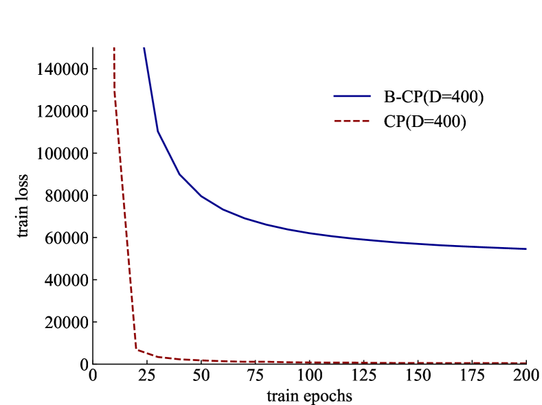
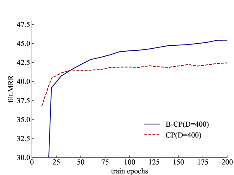
Figure 3: Training loss and filtered MRR vs. epochs trained on WN18RR.

We compared standard DistMult/CP and B-DistMult/B-CP models with other state-of-the-art KGE models. The best vector dimensions were 200 in DistMult/CP for all datasets, while the best resulting vector dimensions of B-DistMult/B-CP for WN18/WN18RR/FB15k-237 were 400 and those for FB15k were 800. Table 3 shows the results on WN18 and FB15k, and Table 4 shows the results on WN18RR and FB15k-237. For most evaluation metrics, the proposed B-CP model outperformed or was competitive with the best baseline. However, with a small vector dimension ($D=200$), B-CP’s performance tended to degrade.

Figure 3 shows training loss and accuracy versus training epochs for CP ($D=400$) and B-CP ($D=400$) on WN18RR. The results indicate that CP is prone to overfitting as the training epochs increase. In contrast, B-CP appears less susceptible to overfitting than CP.

6.1.4 KGC Performance vs. Model Size

Table 5: Results on WN18RR and FB15k-237 with varying embedding dimensions. Model size denotes the number of bits required to store the model in memory.

Model	Model Size	MRR
		WN18RR	FB15k-237
CP ($D=15$)	$480(2N_{e}+N_{r})$	40.0	22.0
CP ($D=50$)	$1,600(2N_{e}+N_{r})$	43.0	24.8
CP ($D=200$)	$6,400(2N_{e}+N_{r})$	44.0	29.0
VQ-CP ($D=200$)	$200(2N_{e}+N_{r})$	36.0	8.7
VQ-CP ($D=400$)	$400(2N_{e}+N_{r})$	36.0	8.3
B-CP ($D=100$)	$100(2N_{e}+N_{r})$	38.0	23.2
B-CP ($D=200$)	$200(2N_{e}+N_{r})$	45.0	27.8
B-CP ($D=300$)	$300(2N_{e}+N_{r})$	45.0	29.0
B-CP ($D=400$)	$400(2N_{e}+N_{r})$	46.0	29.2
B-CP ($D=800$)	$800(2N_{e}+N_{r})$	46.0	29.5

We also investigated the extent to which the proposed B-CP method can reduce model size and maintain KGC performance. For a fair evaluation, we also examined a naive vector quantization method (VQ) [32] that can reduce the model size. Given a real valued matrix ${\bm{\mathbf{X}}}\in\mathbb{R}^{D_{1}\times D_{2}}$, the VQ method solves the following optimization problem:

$${\hat{\bm{\mathbf{X}}}^{(\text{b})}},{\hat{\alpha}}=\mathop{\rm argmin}\limits_{{\bm{\mathbf{X}}}^{(\text{b})},\alpha}{\|{\bm{\mathbf{X}}}-\alpha{\bm{\mathbf{X}}}^{(\text{b})}\|_{F}^{2}}$$

where ${\bm{\mathbf{X}}}^{(\text{b})}\in\{+1,-1\}^{D_{1}\times D_{2}}$ is a binary matrix and $\alpha$ is a positive real value. The optimal solutions ${\hat{\bm{\mathbf{X}}}^{(\text{b})}}$ and ${\hat{\alpha}}$ are given by $Q_{1}({\bm{\mathbf{X}}})$ and $\frac{1}{D_{1}\times D_{2}}\|{\bm{\mathbf{X}}}\|_{1}$, respectively, where $\|\cdot\|_{1}$ denotes $l_{1}$-norm, and $Q_{1}({\bm{\mathbf{X}}})$ is a sign function whose behavior in each element $x$ of ${\bm{\mathbf{X}}}$ is as per the sign function $Q_{1}(x)$. After obtaining factor matrices ${\bm{\mathbf{A}}}$, ${\bm{\mathbf{B}}},$ and ${\bm{\mathbf{C}}}$ via CP decomposition, we solved the above optimization problem independently for each matrix. We refer to this method as VQ-CP.

Table 5 shows the results when the dimension size of the embeddings was varied. While CP requires $64\times D$ and $32\times D$ bits per entity and relation, respectively, both B-CP and VQ-CP only require one thirty-second of these bit values. Obviously, the task performance dropped significantly after vector quantization (VQ-CP). The CP performance also degraded when the vector dimension was reduced from 200 to 15 or 50. While simply reducing the number of dimensions degraded accuracy, B-CP successfully reduced the model size nearly 10- to 20-fold compared to CP and other KGE models without performance degradation.

6.1.5 Computation Time

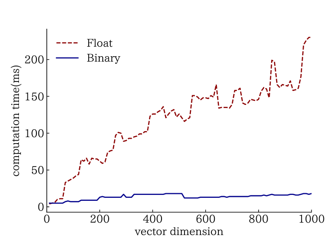
Figure 4: CPU run time per 100,000-times score computations with single CPU thread.

As described in Section 5, the B-CP model can accelerate the computation of confidence scores by using the XNOR operation and Hamming distance function. To compare the score computation speed between CP (Float) and B-CP (Binary), we calculated the confidence scores 100,000 times for both CP and B-CP while varying the vector size $D$ from 10 to 1,000 at increments of ten. Figure 4 clearly shows that bitwise operations increase computation speed significantly compared to standard multiply-accumulate operations.

6.2 Evaluation on Large-scale Knowledge Graphs

Table 6: Freebase-music and YAGO statistics.

	Freebase-music	YAGO
$N_{e}$	3,004,505	3,983,941
$N_{r}$	131	75
# training triples	14,786,254	9,944,560
# validation triples	3,696,564	2,486,140
# test triples	3,696,564	2,486,140

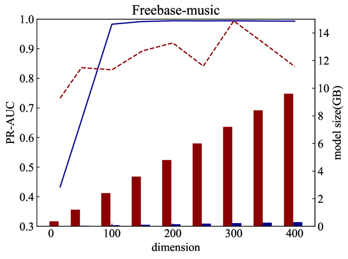
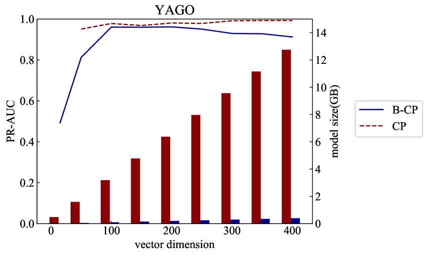
Figure 5: Results of CP and B-CP models on Freebase-music and YAGO datasets. The line and bar graphs represent PR-AUC and model size, respectively. CP model results ($D=15$) on YAGO were excluded because minimization of the loss function did not converge at all.

To verify the effectiveness of B-CP over larger datasets, we also conducted experiments on the Freebase-music [11] and YAGO [34] datasets. To reduce noises in Freebase-music, we removed the triples whose relations and entities occur less than ten times, and in YAGO we used only fact triples and excluded other extra information, such as taxonomies and types of entities. In both datasets, we split the triples into 80/10/10 fractions for training, validation, and testing. Furthermore, we randomly generated the same number of triples as test (validation) triples that were not in the knowledge graph, and added generated triples to the test (validation) triples as negative samples. Table 6 shows the data statistics.

We tried all combinations of $\lambda_{A},\lambda_{B},\lambda_{C}\in\{0.0001,0\}$, learning rate $\eta\in\{0.005,0.0075,0.01,0.025,0.05\}$, and embedding dimension $D\in\{15,50,\linebreak 100,150,200,250,300,350,400\}$ during the grid search. We evaluated the results using the area under the precision-recall curve (PR-AUC).

The results are shown in Figure 5. As expected, on each dataset, B-CP successfully reduced the model size while achieving performance equal to or better than CP. These results show that B-CP is robust to data size.

6.3 Link-Based Entity Clustering

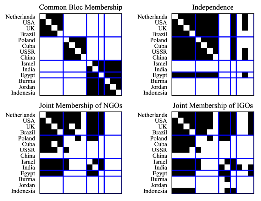
Figure 6: Country clusters in the Nations dataset. Each black entry indicates an existing relation between two countries.

Clustering is a useful technique to assess natural groupings of various data items, including entities in relational databases. Such cluster information assists knowledge engineers in the automatic construction of taxonomies from instance data [30]. In this section, we demonstrate the utility of B-CP in link-based clustering of the Nations dataset [14].

The Nations dataset contains 2,024 triples composed of 14 countries and 56 relations. Experiments were conducted under the same hyperparameters that achieved the best results on the WN18 dataset. We applied hierarchical clustering to a factor matrix $\bm{\mathbf{A}}^{(\text{b})}$ and divided entities into five clusters, using the single linkage method with Euclidean distance. Euclidean distance between binary vectors $\bm{\mathbf{p}}^{(\text{b})}$ and $\bm{\mathbf{q}}^{(\text{b})}$ can be computed as follows using Hamming distance,

$$d(\bm{\mathbf{p}}^{(\text{b})},\bm{\mathbf{q}}^{(\text{b})})=\sqrt{\sum_{i=1}^{N}{(p_{i}^{(\text{b})}-q_{i}^{(\text{b})})^{2}}}=2\sqrt{h(\overline{\bm{\mathbf{p}}}^{(\text{b})},\overline{\bm{\mathbf{q}}}^{(\text{b})})}$$

which accelerates the computation of clustering.

We show the clustering results in Figure 6. The countries are partitioned into one group from the western bloc, one group from the communist bloc, and three groups for the neutral bloc. The four relations in Figure 6 show that this is a reasonable partitioning of Nations dataset, which indicate that B-CP can accurately represent the semantic relationships between entities in binary vector space.

7 Conclusion

In this paper, we have shown that it is possible to obtain binary vectors of entities and relations in knowledge graphs that take $10$–$20$ times less storage/memory than the original representations with floating-point numbers. In addition, with bitwise operations, the time required to compute scores was reduced considerably. Tensor factorization occurs in many machine learning applications, such as item recommendation [31] and web link analysis [17]. Applying the proposed B-CP algorithm to the analysis of other relational datasets is an interesting avenue for future work.

Appendix A Proof of Theorem 1

In this appendix, we prove the full expressiveness of B-CP, which was stated as Theorem 1 without proof in Section 5.3. To this end, for a given knowledge graph (or more precisely, its boolean tensor $\bm{\mathbf{\mathcal{X}}}$ representing the truth values), we define a specific B-CP model, denoted by $\text{BCP}_{\Delta}^{*}(\bm{\mathbf{\mathcal{X}}})$, and show that it indeed faithfully represents $\bm{\mathbf{\mathcal{X}}}$ by Eq. (3) for a certain $\Delta$.

Definition A.1.

Let $\bm{\mathbf{\mathcal{X}}}\in\{0,1\}^{N_{e}\times N_{e}\times N_{r}}$ be an arbitrary boolean tensor. Let $\text{BCP}_{\Delta}^{*}(\bm{\mathbf{\mathcal{X}}})=(\bm{\mathbf{A}}^{(\text{b})},\bm{\mathbf{B}}^{(\text{b})},\bm{\mathbf{C}}^{(\text{b})})$, where binary matrices $\bm{\mathbf{A}}^{(\text{b})},\bm{\mathbf{B}}^{(\text{b})}\in\{+\Delta,-\Delta\}^{N_{e}\times 8N_{e}N_{r}}$, and $\bm{\mathbf{C}}^{(\text{b})}\in\{+\Delta,-\Delta\}^{N_{r}\times 8N_{e}N_{r}}$ are defined as follows.

• All three matrices are block matrices of $4$-dimensional binary row vectors, each of which is either one of

  $$\bm{\mathbf{p}} =[+\Delta,+\Delta,-\Delta,-\Delta],$$ (4)

  $$\bm{\mathbf{q}} =[+\Delta,-\Delta,+\Delta,-\Delta],$$ (5)

  $$\bm{\mathbf{r}} =[+\Delta,+\Delta,+\Delta,+\Delta],$$ (6)

  or $-\bm{\mathbf{r}}$. In other words, $\bm{\mathbf{A}}^{(\text{b})}=[\bm{\mathbf{a}}^{(\text{b})}_{mn}]_{m\in[N_{e}],n\in[2N_{e}N_{r}]}$, $\bm{\mathbf{B}}^{(\text{b})}=[\bm{\mathbf{b}}^{(\text{b})}_{mn}]_{m\in[N_{e}],n\in[2N_{e}N_{r}]}$, and $\bm{\mathbf{C}}^{(\text{b})}=[\bm{\mathbf{c}}^{(\text{b})}_{mn}]_{m\in[N_{r}],n\in[2N_{e}N_{r}]}$, where $\bm{\mathbf{a}}^{(\text{b})}_{mn},\bm{\mathbf{b}}^{(\text{b})}_{mn},\bm{\mathbf{c}}^{(\text{b})}_{mn}\in\{\bm{\mathbf{p}},\bm{\mathbf{q}},\bm{\mathbf{r}},-\bm{\mathbf{r}}\}$.

• For each $i\in[N_{e}]$ and $\gamma\in[2N_{e}N_{r}]$,

  $$\bm{\mathbf{a}}_{i\gamma}^{(\text{b})}=\begin{cases}\bm{\mathbf{p}}&\text{if }(\gamma{\rm~{}mod~{}}N_{e})=(i{\rm~{}mod~{}}N_{e}),\\ \bm{\mathbf{q}}&\text{otherwise.}\end{cases}$$ (7)

• Let $\iota(\gamma)=(((\gamma-1)\bmod 2N_{e})\bmod N_{e})+1$ and $\kappa(\gamma)=\lfloor(\gamma-1)/2N_{e}\rfloor+1$. For each $j\in[N_{e}]$ and $\gamma\in[2N_{e}N_{r}]$,

  $$\bm{\mathbf{b}}_{j\gamma}^{(\text{b})}=\begin{cases}\bm{\mathbf{p}}&\text{if }x_{\iota(\gamma)j\kappa(\gamma)}=1,\\ \bm{\mathbf{r}}&\text{otherwise.}\end{cases}$$ (8)

• For each $k\in[N_{r}]$ and $\gamma\in[2N_{e}N_{r}]$,

  $$\bm{\mathbf{c}}_{k\gamma}^{(\text{b})}=\begin{cases}\bm{\mathbf{r}}&\text{if }(\gamma-1)\bmod 2N_{e}<N_{e}\text{ or }\left\lfloor(\gamma-1)/2N_{e}\right\rfloor+1=k,\\ -\bm{\mathbf{r}}&{\rm otherwise.}\end{cases}$$ (9)

Figure 1: Regularities in $\bm{\mathbf{A}}^{(\text{b})}$ and $\bm{\mathbf{C}}^{(\text{b})}$ of $\text{BCP}^{*}_{\Delta}(\bm{\mathbf{\mathcal{X}}})$. Solid vertical lines separate “pages,” and dotted lines separate “halfpages” within each page. Matrix $\bm{\mathbf{B}}^{(\text{b})}$ also shows some regularities; see Lemma A.1(d). It is not depicted here as its elements are dependent on $\bm{\mathbf{\mathcal{X}}}$.

Figure 1 illustrates the binary factor matrices of Definition A.1. As seen from the figure, each row of the matrices exhibits a certain pattern every $2N_{e}$ blocks, which we call a page. Each page can further be divided into a pair of halfpages consisting of $N_{e}$ blocks each, which also show periodic patterns. These patterns are stated precisely in Lemma A.1 below. It extensively uses addressing functions $\alpha(k,m)=2N_{e}(k-1)+m$ and $\beta(k,m)=\alpha(k,m)+N_{e}$ to specify the position of an individual block within the page it belongs to; function $\alpha(k,m)$ designates the $m$th block within the first halfpage of the $k$th page, whereas $\beta(k,m)$ designates the $m$th block in the second halfpage. There is a one-to-one correspondence between linear addressing by $\gamma\in[2N_{e}N_{r}]$ and 2-dimensional indexing by $k\in[N_{r}]$ and $m\in[N_{e}]$, combined with $\alpha$ and $\beta$ to specify a halfpage.

Lemma A.1.

Let $\bm{\mathbf{p}}$, $\bm{\mathbf{q}}$, and $\bm{\mathbf{r}}$ be as given by Eqs. (4)–(6). The following statements (a)–(f) hold for block matrices $\bm{\mathbf{A}}^{(\text{b})}=[\bm{\mathbf{a}}^{(\text{b})}_{mn}]$, $\bm{\mathbf{B}}^{(\text{b})}=[\bm{\mathbf{b}}^{(\text{b})}_{mn}]$, $\bm{\mathbf{C}}^{(\text{b})}=[\bm{\mathbf{c}}^{(\text{b})}_{mn}]$, where $(\bm{\mathbf{A}}^{(\text{b})}$, $\bm{\mathbf{B}}^{(\text{b})}$, $\bm{\mathbf{C}}^{(\text{b})})=\text{BCP}_{\Delta}^{*}(\bm{\mathbf{\mathcal{X}}})$ is given by Definition A.1.

1. For any $i\in[N_{e}]$ and $\gamma\in[(2N_{r}-1)N_{e}]$,

   $$\bm{\mathbf{a}}^{(\text{b})}_{i\gamma}=\bm{\mathbf{a}}^{(\text{b})}_{i,(\gamma+N_{e})}.$$ (10)

   In particular, for any $i,m\in[N_{e}]$ and $k\in[N_{r}]$,

   $$\bm{\mathbf{a}}^{(\text{b})}_{i\alpha(k,m)}=\bm{\mathbf{a}}^{(\text{b})}_{i\beta(k,m)}.$$ (11)

2. For any $i\in[N_{e}]$ and $k\in[N_{r}]$,

   $$\bm{\mathbf{a}}^{(\text{b})}_{i\alpha(k,i)}=\bm{\mathbf{p}}.$$ (12)

3. For any $i\in[N_{e}]$, $m^{\prime}\in[N_{e}]\backslash\{i\}$, and $k\in[N_{r}]$,

   $$\bm{\mathbf{a}}^{(\text{b})}_{i\alpha(k,m^{\prime})}=\bm{\mathbf{q}}.$$ (13)

4. For any $j,m\in[N_{e}]$ and $k\in[N_{r}]$,

   $$\bm{\mathbf{b}}^{(\text{b})}_{j\alpha(k,m)}=\bm{\mathbf{b}}^{(\text{b})}_{j\beta(k,m)}.$$ (14)

5. For any $k\in[N_{r}]$ and $m\in[N_{e}]$,

   $$\bm{\mathbf{c}}_{k\alpha(k,m)}^{(\text{b})}=\bm{\mathbf{c}}_{k\beta(k,m)}^{(\text{b})}=\bm{\mathbf{r}}.$$ (15)

6. For any $k\in[N_{r}],m\in[N_{e}]$ and $n^{\prime}\in[N_{r}]\backslash\{k\}$,

   $$\bm{\mathbf{c}}_{k\alpha(n^{\prime},m)}^{(\text{b})}=-\bm{\mathbf{c}}_{k\beta(n^{\prime},m)}^{(\text{b})}.$$ (16)

Proof.

1. The statement follows from $(\gamma\bmod N_{e})=((\gamma+N_{e})\bmod N_{e})$ and the definition of $\bm{\mathbf{a}}^{(\text{b})}$ given by Eq. (7).

2. Follows from $\alpha(k,i)\bmod N_{e}=i$ and Eq. (7).

3. Follows from $\alpha(k,m^{\prime})\bmod N_{e}\neq i$ (because $m^{\prime}\in[N_{e}]\backslash\{i\}$) and Eq. (7).

4. Follows from $m=\iota(\alpha(n,m))=\iota(\beta(n,m))$ and $n=\kappa(\alpha(n,m))=\kappa(\beta(n,m))$.

5. Follows from Eq. (9).

6. Follows from Eq. (9), specifically, $\bm{\mathbf{c}}_{k\alpha(n^{\prime},m)}^{(\text{b})}=\bm{\mathbf{r}}$ and $\bm{\mathbf{c}}_{k\beta(n^{\prime},m)}^{(\text{b})}=-\bm{\mathbf{r}}$. ∎

The following corollary is a direct consequence of Lemma A.1.

Corollary A.1.

For any $i,j\in[N_{e}]$ and $k\in[N_{r}]$,

$$(\bm{\mathbf{a}}_{i\alpha(k,i)}^{(\text{b})}\circ\bm{\mathbf{b}}_{j\alpha(k,i)}^{(\text{b})})\bm{\mathbf{c}}_{k\alpha(k,i)}^{(b)\mathrm{T}}=(\bm{\mathbf{a}}_{i\beta(k,i)}^{(\text{b})}\circ\bm{\mathbf{b}}_{j\beta(k,i)}^{(\text{b})})\bm{\mathbf{c}}_{k\beta(k,i)}^{(b)\mathrm{T}}.$$

From Lemma A.1(a), (d), and (f), we also have the following.

Corollary A.2.

For any $i,j,m\in[N_{e}]$, $k\in[N_{r}]$, and $n^{\prime}\in[N_{r}]\backslash\{k\}$,

$$(\bm{\mathbf{a}}_{i\alpha(n^{\prime},m)}^{(\text{b})}\circ\bm{\mathbf{b}}_{j\alpha(n^{\prime},m)}^{(\text{b})})\bm{\mathbf{c}}_{k\alpha(n^{\prime},m)}^{(b)\mathrm{T}}+(\bm{\mathbf{a}}_{i\beta(n^{\prime},m)}^{(\text{b})}\circ\bm{\mathbf{b}}_{j\beta(n^{\prime},m)}^{(\text{b})})\bm{\mathbf{c}}_{k\beta(n^{\prime},m)}^{(b)\mathrm{T}}=0.$$

These lemmas and corollaries lead to the following:

Lemma A.2.

For any $i,j\in[N_{e}]$ and $k\in[N_{r}]$,

$$\sum_{\gamma\in[2N_{e}N_{r}]\backslash\{\alpha(k,i),\beta(k,i)\}}\!\!\!\!\!\!\!\!\!\!\!\!(\bm{\mathbf{a}}_{i\gamma}^{(\text{b})}\circ\bm{\mathbf{b}}_{j\gamma}^{(\text{b})})\bm{\mathbf{c}}_{k\gamma}^{(b)\mathrm{T}}=0.$$

Proof.

Let $\bm{\mathbf{p}}$, $\bm{\mathbf{q}}$, and $\bm{\mathbf{r}}$ be as given by Eqs. (4)–(6). From Lemma A.1(a), (c), (d), and (e), we have for any $m^{\prime}\in[N_{e}]\backslash\{i\}$,

$$\bm{\mathbf{a}}_{i,\alpha(k,m^{\prime})}^{(\text{b})} =\bm{\mathbf{a}}_{i,\beta(k,m^{\prime})}^{(\text{b})}=\bm{\mathbf{q}},$$

$$\bm{\mathbf{b}}_{j,\alpha(k,m^{\prime})}^{(\text{b})} =\bm{\mathbf{b}}_{j,\beta(k,m^{\prime})}^{(\text{b})},$$

$$\bm{\mathbf{c}}_{k,\alpha(k,m^{\prime})}^{(\text{b})} =\bm{\mathbf{c}}_{k,\beta(k,m^{\prime})}^{(\text{b})}=\bm{\mathbf{r}}.$$

Thus, for any $m^{\prime}\in[N_{e}]\backslash\{i\}$,

$$(\bm{\mathbf{a}}_{i\alpha(k,m^{\prime})}^{(\text{b})}\circ\bm{\mathbf{b}}_{j\alpha(k,m^{\prime})}^{(\text{b})})\bm{\mathbf{c}}_{k\alpha(k,m^{\prime})}^{(b)\mathrm{T}} =(\bm{\mathbf{a}}_{i\beta(k,m^{\prime})}^{(\text{b})}\circ\bm{\mathbf{b}}_{j\beta(k,m^{\prime})}^{(\text{b})})\bm{\mathbf{c}}_{k\beta(k,m^{\prime})}^{(b)\mathrm{T}}$$

$$=(\bm{\mathbf{q}}\circ\bm{\mathbf{b}}_{j\alpha(k,m^{\prime})}^{(\text{b})})\bm{\mathbf{r}}^{\mathrm{T}}$$

$$=0.$$ (17)

The last equality holds because $\bm{\mathbf{b}}_{j\alpha(k,m^{\prime})}^{(\text{b})}$ is either $\bm{\mathbf{p}}$ or $\bm{\mathbf{r}}$ by definition, and $(\bm{\mathbf{q}}\circ\bm{\mathbf{p}})\bm{\mathbf{r}}^{\mathrm{T}}=(\bm{\mathbf{q}}\circ\bm{\mathbf{r}})\bm{\mathbf{r}}^{\mathrm{T}}=0$.

Now, for any $i,j\in[N_{e}]$ and $k\in[N_{r}]$,

$$\sum_{\gamma\in[2N_{e}N_{r}]\backslash\{\alpha(k,i),\beta(k,i)\}}\!\!\!\!\!\!\!\!(\bm{\mathbf{a}}_{i\gamma}^{(\text{b})}\circ\bm{\mathbf{b}}_{j\gamma}^{(\text{b})})\bm{\mathbf{c}}_{k\gamma}^{(b)\mathrm{T}}$$

$$=\!\!\!\!\sum_{\begin{subarray}{c}n^{\prime}\in[N_{r}]\backslash\{k\}\\ m\in[N_{e}]\end{subarray}}\underbrace{\left((\bm{\mathbf{a}}_{i\alpha(n^{\prime},m)}^{(\text{b})}\circ\bm{\mathbf{b}}_{j\alpha(n^{\prime},m)}^{(\text{b})})\bm{\mathbf{c}}_{k\alpha(n^{\prime},m)}^{(b)\mathrm{T}}+(\bm{\mathbf{a}}_{i\beta(n^{\prime},m)}^{(\text{b})}\circ\bm{\mathbf{b}}_{j\beta(n^{\prime},m)}^{(\text{b})})\bm{\mathbf{c}}_{k\beta(n^{\prime},m)}^{(b)\mathrm{T}}\right)}_{=0\;\text{\hbox to0.0pt{ by Cororally~{}\ref{cor:zero-sum-abc}\hss}}}$$

$$\quad+\!\!\!\!\sum_{m^{\prime}\in[N_{e}]\backslash\{i\}}\underbrace{\left((\bm{\mathbf{a}}_{i\alpha(k,m^{\prime})}^{(\text{b})}\circ\bm{\mathbf{b}}_{j\alpha(k,m^{\prime})}^{(\text{b})})\bm{\mathbf{c}}_{k\alpha(k,m^{\prime})}^{(b)\mathrm{T}}+(\bm{\mathbf{a}}_{i\beta(k,m^{\prime})}^{(\text{b})}\circ\bm{\mathbf{b}}_{j\beta(k,m^{\prime})}^{(\text{b})})\bm{\mathbf{c}}_{k\beta(k,m^{\prime})}^{(b)\mathrm{T}}\right)}_{=0\;\text{\hbox to0.0pt{ by Eq.~{}\eqref{eq:zero-abc}\hss}}}$$

$$=0.\qed$$

We are now ready to prove Theorem 1, restated here as Theorem A.1.

Theorem A.1 (Theorem 1; full expressiveness of B-CP).

For an arbitrary binary tensor $\bm{\mathbf{\mathcal{X}}}\in\{0,1\}^{N_{e}\times N_{e}\times N_{r}}$, there exists a B-CP decomposition with binary factor matrices $\bm{\mathbf{A}}^{(\text{b})},\bm{\mathbf{B}}^{(\text{b})}\in\{+\Delta,-\Delta\}^{N_{e}\times D}$ and $\bm{\mathbf{C}}^{(\text{b})}\in\{+\Delta,-\Delta\}^{N_{r}\times D}$ for some $D$ and $\Delta$, such that

$$\bm{\mathbf{\mathcal{X}}}=\sum_{d\in[D]}\bm{\mathbf{a}}^{(\text{b})}_{d}\otimes\bm{\mathbf{b}}^{(\text{b})}_{d}\otimes\bm{\mathbf{c}}^{(\text{b})}_{d}.$$ (18)

Proof.

Let $\Delta=1/2$ and let $(\bm{\mathbf{A}}^{(\text{b})},\bm{\mathbf{B}}^{(\text{b})},\bm{\mathbf{C}}^{(\text{b})})=\text{BCP}_{\Delta}^{*}(\bm{\mathbf{\mathcal{X}}})$ given by Definition A.1. We show that these matrices indeed satisfy Eq. (18).

For any $i,j\in[N_{e}]$ and $k\in[N_{r}]$, the score $\theta_{ijk}$ for triple $(e_{i},e_{j},r_{k})$ is:

$$\theta_{ijk} =(\bm{\mathbf{a}}_{i:}^{(\text{b})}\circ\bm{\mathbf{b}}_{j:}^{(\text{b})})\bm{\mathbf{c}}_{k:}^{(b)\mathrm{T}}$$

$$=\sum_{\gamma\in[2N_{e}N_{r}]}(\bm{\mathbf{a}}_{i\gamma}^{(\text{b})}\circ\bm{\mathbf{b}}_{j\gamma}^{(\text{b})})\bm{\mathbf{c}}_{k\gamma}^{(b)\mathrm{T}}$$

$$=(\bm{\mathbf{a}}_{i\alpha(k,i)}^{(\text{b})}\circ\bm{\mathbf{b}}_{j\alpha(k,i)}^{(\text{b})})\bm{\mathbf{c}}_{k\alpha(k,i)}^{(b)\mathrm{T}}$$

$$\qquad+\underbrace{(\bm{\mathbf{a}}_{i\beta(k,i)}^{(\text{b})}\circ\bm{\mathbf{b}}_{j\beta(k,i)}^{(\text{b})})\bm{\mathbf{c}}_{k\beta(k,i)}^{(b)\mathrm{T}}}_{=(\bm{\mathbf{a}}_{i\alpha(k,i)}^{(\text{b})}\circ\bm{\mathbf{b}}_{j\alpha(k,i)}^{(\text{b})})\bm{\mathbf{c}}_{k\alpha(k,i)}^{(b)\mathrm{T}}\text{ by Corollary~{}\ref{cor:alpha-beta-terms-are-equal}}}+\underbrace{\sum_{\gamma\neq\alpha(k,i),\beta(k,i)}\!\!\!\!(\bm{\mathbf{a}}_{i\gamma}^{(\text{b})}\circ\bm{\mathbf{b}}_{j\gamma}^{(\text{b})})\bm{\mathbf{c}}_{k\gamma}^{(b)\mathrm{T}}}_{=0\text{ by Lemma~{}\ref{lem:sum-of-remaining-terms-are-null}}}$$

$$=2(\bm{\mathbf{a}}_{i\alpha(k,i)}^{(\text{b})}\circ\bm{\mathbf{b}}_{j\alpha(k,i)}^{(\text{b})})\bm{\mathbf{c}}_{k\alpha(k,i)}^{(b)\mathrm{T}}.$$ (19)

Let $\bm{\mathbf{p}},\bm{\mathbf{q}},\bm{\mathbf{r}}\in\{+\Delta,-\Delta\}^{1\times 4}$ be as given by Eqs. (4)–(6). For any $i,j\in[N_{e}]$ and $k\in[N_{r}]$, if $x_{ijk}=1$, $\bm{\mathbf{b}}_{j\alpha(k,i)}^{(\text{b})}=\bm{\mathbf{p}}$ by Eq. (8), and the following equation holds:

$$\theta_{ijk} =2(\bm{\mathbf{a}}_{i\alpha(k,i)}^{(\text{b})}\circ\bm{\mathbf{b}}_{j\alpha(k,i)}^{(\text{b})})\bm{\mathbf{c}}_{k\alpha(k,i)}^{(b)\mathrm{T}} \because\text{ Eq.~{}\eqref{eq:score-breakdown}}$$

$$=2(\bm{\mathbf{p}}\circ\bm{\mathbf{p}})\bm{\mathbf{r}}^{\mathrm{T}} \because\text{ Lemma~{}\ref{lem:faithful-encoding-periodicity}\ref{itm:a-alpha}, \ref{itm:c-periodicity}}$$

$$=8\Delta^{3}$$

$$=1\;(=x_{ijk}). \because\Delta=1/2$$ (20)

And if $x_{ijk}=0$, $\bm{\mathbf{b}}_{j\alpha(k,i)}^{(\text{b})}=\bm{\mathbf{r}}$, and we have:

$$\theta_{ijk} =2(\bm{\mathbf{a}}_{i\alpha(k,i)}^{(\text{b})}\circ\bm{\mathbf{b}}_{j\alpha(k,i)}^{(\text{b})})\bm{\mathbf{c}}_{k\alpha(k,i)}^{(b)\mathrm{T}} \because\text{ Eq.~{}\eqref{eq:score-breakdown}}$$

$$=2(\bm{\mathbf{p}}\circ\bm{\mathbf{r}})\bm{\mathbf{r}}^{\mathrm{T}} \because\text{ Lemma~{}\ref{lem:faithful-encoding-periodicity}\ref{itm:a-alpha}, \ref{itm:c-periodicity}}$$

$$=0\;(=x_{ijk}).$$ (21)

By Eqs. (20) and (21), $x_{ijk}=\theta_{ijk}$ holds irrespective of the value of $x_{ijk}$. Hence, $\bm{\mathbf{\mathcal{X}}}=\sum_{d\in[D]}\bm{\mathbf{a}}_{d}^{(\text{b})}\otimes\bm{\mathbf{b}}_{d}^{(\text{b})}\otimes\bm{\mathbf{c}}_{d}^{(\text{b})}$ where $D=8N_{e}N_{r}$. ∎

References

• Bengio et al. [2013] Bengio, Y., Léonard, N., Courville, A.C., 2013. Estimating or propagating gradients through stochastic neurons for conditional computation. CoRR abs/1308.3432. arXiv:1308.3432.
• Bollacker et al. [2008] Bollacker, K.D., Evans, C., Paritosh, P., Sturge, T., Taylor, J., 2008. Freebase: a collaboratively created graph database for structuring human knowledge, in: Proceedings of the ACM SIGMOD International Conference on Management of Data, SIGMOD 2008, Vancouver, BC, Canada, June 10-12, 2008, pp. 1247–1250.
• Bordes et al. [2014] Bordes, A., Chopra, S., Weston, J., 2014. Question answering with subgraph embeddings, in: Proceedings of the 2014 Conference on Empirical Methods in Natural Language Processing, EMNLP 2014, October 25-29, 2014, Doha, Qatar, A meeting of SIGDAT, a Special Interest Group of the ACL, pp. 615–620.
• Bordes et al. [2013] Bordes, A., Usunier, N., García-Durán, A., Weston, J., Yakhnenko, O., 2013. Translating embeddings for modeling multi-relational data, in: Advances in Neural Information Processing Systems 26: 27th Annual Conference on Neural Information Processing Systems 2013. Proceedings of a meeting held December 5-8, 2013, Lake Tahoe, Nevada, United States., pp. 2787–2795.
• Courbariaux et al. [2015] Courbariaux, M., Bengio, Y., David, J., 2015. Binaryconnect: Training deep neural networks with binary weights during propagations, in: Advances in Neural Information Processing Systems 28: Annual Conference on Neural Information Processing Systems 2015, December 7-12, 2015, Montreal, Quebec, Canada, pp. 3123–3131.
• Dettmers et al. [2018] Dettmers, T., Minervini, P., Stenetorp, P., Riedel, S., 2018. Convolutional 2d knowledge graph embeddings, in: Proceedings of the Thirty-Second AAAI Conference on Artificial Intelligence, New Orleans, Louisiana, USA, February 2-7, 2018.
• Glorot and Bengio [2010] Glorot, X., Bengio, Y., 2010. Understanding the difficulty of training deep feedforward neural networks, in: Proceedings of the Thirteenth International Conference on Artificial Intelligence and Statistics, AISTATS 2010, Chia Laguna Resort, Sardinia, Italy, May 13-15, 2010, pp. 249–256.
• Guo [2018] Guo, Y., 2018. A survey on methods and theories of quantized neural networks. CoRR abs/1808.04752. arXiv:1808.04752.
• Hayashi and Shimbo [2017] Hayashi, K., Shimbo, M., 2017. On the equivalence of holographic and complex embeddings for link prediction, in: Proceedings of the 55th Annual Meeting of the Association for Computational Linguistics, ACL 2017, Vancouver, Canada, July 30 - August 4, Volume 2: Short Papers, pp. 554–559.
• Hitchcock [1927] Hitchcock, F.L., 1927. The expression of a tensor or a polyadic as a sum of products. J. Math. Phys 6, 164–189.
• Jeon et al. [2015] Jeon, I., Papalexakis, E.E., Kang, U., Faloutsos, C., 2015. Haten2: Billion-scale tensor decompositions, in: 31st IEEE International Conference on Data Engineering, ICDE 2015, Seoul, South Korea, April 13-17, 2015, pp. 1047–1058.
• Kadlec et al. [2017] Kadlec, R., Bajgar, O., Kleindienst, J., 2017. Knowledge base completion: Baselines strike back, in: Proceedings of the 2nd Workshop on Representation Learning for NLP, Rep4NLP@ACL 2017, Vancouver, Canada, August 3, 2017, pp. 69–74.
• Kazemi and Poole [2018] Kazemi, S.M., Poole, D., 2018. Simple embedding for link prediction in knowledge graphs, in: Advances in Neural Information Processing Systems 31: Annual Conference on Neural Information Processing Systems 2018, NeurIPS 2018, 3-8 December 2018, Montréal, Canada., pp. 4289–4300.
• Kemp et al. [2006] Kemp, C., Tenenbaum, J.B., Griffiths, T.L., Yamada, T., Ueda, N., 2006. Learning systems of concepts with an infinite relational model, in: Proceedings, The Twenty-First National Conference on Artificial Intelligence and the Eighteenth Innovative Applications of Artificial Intelligence Conference, July 16-20, 2006, Boston, Massachusetts, USA, pp. 381–388.
• Kishimoto et al. [2019] Kishimoto, K., Hayashi, K., Akai, G., Shimbo, M., Komatani, K., 2019. Binarized knowledge graph embeddings, in: Advances in Information Retrieval - 41st European Conference on IR Research, ECIR 2019, Cologne, Germany, April 14-18, 2019, Proceedings, Part I, pp. 181–196.
• Kolda and Bader [2009] Kolda, T.G., Bader, B.W., 2009. Tensor decompositions and applications. SIAM Review 51, 455–500.
• Kolda et al. [2005] Kolda, T.G., Bader, B.W., Kenny, J.P., 2005. Higher-order web link analysis using multilinear algebra, in: Proceedings of the 5th IEEE International Conference on Data Mining (ICDM 2005), 27-30 November 2005, Houston, Texas, USA, pp. 242–249.
• Lacroix et al. [2018] Lacroix, T., Usunier, N., Obozinski, G., 2018. Canonical tensor decomposition for knowledge base completion, in: Proceedings of the 35th International Conference on Machine Learning, ICML 2018, Stockholmsmässan, Stockholm, Sweden, July 10-15, 2018, pp. 2869–2878.
• Lam [2018] Lam, M., 2018. Word2bits - quantized word vectors. CoRR abs/1803.05651. arXiv:1803.05651.
• Lin et al. [2015] Lin, Y., Liu, Z., Sun, M., Liu, Y., Zhu, X., 2015. Learning entity and relation embeddings for knowledge graph completion, in: Proceedings of the Twenty-Ninth AAAI Conference on Artificial Intelligence, January 25-30, 2015, Austin, Texas, USA., pp. 2181–2187.
• Liu et al. [2017] Liu, H., Wu, Y., Yang, Y., 2017. Analogical inference for multi-relational embeddings, in: Proceedings of the 34th International Conference on Machine Learning, ICML 2017, Sydney, NSW, Australia, 6-11 August 2017, pp. 2168–2178.
• Ma et al. [2015] Ma, Y., Crook, P.A., Sarikaya, R., Fosler-Lussier, E., 2015. Knowledge graph inference for spoken dialog systems, in: 2015 IEEE International Conference on Acoustics, Speech and Signal Processing, ICASSP 2015, South Brisbane, Queensland, Australia, April 19-24, 2015, pp. 5346–5350.
• Manabe et al. [2018] Manabe, H., Hayashi, K., Shimbo, M., 2018. Data-dependent learning of symmetric/antisymmetric relations for knowledge base completion, in: Proceedings of the Thirty-Second AAAI Conference on Artificial Intelligence, New Orleans, Louisiana, USA, February 2-7, 2018.
• Miettinen [2011] Miettinen, P., 2011. Boolean tensor factorizations, in: 11th IEEE International Conference on Data Mining, ICDM 2011, Vancouver, BC, Canada, December 11-14, 2011, pp. 447–456.
• Nguyen et al. [2016] Nguyen, D.Q., Sirts, K., Qu, L., Johnson, M., 2016. Stranse: a novel embedding model of entities and relationships in knowledge bases, in: NAACL HLT 2016, The 2016 Conference of the North American Chapter of the Association for Computational Linguistics: Human Language Technologies, San Diego California, USA, June 12-17, 2016, pp. 460–466.
• Nickel et al. [2016a] Nickel, M., Murphy, K., Tresp, V., Gabrilovich, E., 2016a. A review of relational machine learning for knowledge graphs. Proceedings of the IEEE 104, 11–33.
• Nickel et al. [2016b] Nickel, M., Rosasco, L., Poggio, T.A., 2016b. Holographic embeddings of knowledge graphs, in: Proceedings of the Thirtieth AAAI Conference on Artificial Intelligence, February 12-17, 2016, Phoenix, Arizona, USA., pp. 1955–1961.
• Nickel and Tresp [2013] Nickel, M., Tresp, V., 2013. Logistic tensor factorization for multi-relational data. CoRR abs/1306.2084. arXiv:1306.2084.
• Nickel et al. [2011] Nickel, M., Tresp, V., Kriegel, H., 2011. A three-way model for collective learning on multi-relational data, in: Proceedings of the 28th International Conference on Machine Learning, ICML 2011, Bellevue, Washington, USA, June 28 - July 2, 2011, pp. 809–816.
• Nickel et al. [2012] Nickel, M., Tresp, V., Kriegel, H., 2012. Factorizing YAGO: scalable machine learning for linked data, in: Proceedings of the 21st World Wide Web Conference 2012, WWW 2012, Lyon, France, April 16-20, 2012, pp. 271–280.
• Palumbo et al. [2018] Palumbo, E., Rizzo, G., Troncy, R., Baralis, E., Osella, M., Ferro, E., 2018. An empirical comparison of knowledge graph embeddings for item recommendation, in: Proceedings of the First Workshop on Deep Learning for Knowledge Graphs and Semantic Technologies (DL4KGS) co-located with the 15th Extended Semantic Web Conerence (ESWC 2018), Heraklion, Crete, Greece, June 4, 2018., pp. 14–20.
• Rastegari et al. [2016] Rastegari, M., Ordonez, V., Redmon, J., Farhadi, A., 2016. Xnor-net: Imagenet classification using binary convolutional neural networks, in: Computer Vision - ECCV 2016 - 14th European Conference, Amsterdam, The Netherlands, October 11-14, 2016, Proceedings, Part IV, pp. 525–542.
• Socher et al. [2013] Socher, R., Chen, D., Manning, C.D., Ng, A.Y., 2013. Reasoning with neural tensor networks for knowledge base completion, in: Advances in Neural Information Processing Systems 26: 27th Annual Conference on Neural Information Processing Systems 2013. Proceedings of a meeting held December 5-8, 2013, Lake Tahoe, Nevada, United States., pp. 926–934.
• Suchanek et al. [2007] Suchanek, F.M., Kasneci, G., Weikum, G., 2007. Yago: a core of semantic knowledge, in: Proceedings of the 16th International Conference on World Wide Web, WWW 2007, Banff, Alberta, Canada, May 8-12, 2007, pp. 697–706.
• Trouillon et al. [2016] Trouillon, T., Welbl, J., Riedel, S., Gaussier, É., Bouchard, G., 2016. Complex embeddings for simple link prediction, in: Proceedings of the 33nd International Conference on Machine Learning, ICML 2016, New York City, NY, USA, June 19-24, 2016, pp. 2071–2080.
• Wang et al. [2018] Wang, Y., Gemulla, R., Li, H., 2018. On multi-relational link prediction with bilinear models, in: Proceedings of the Thirty-Second AAAI Conference on Artificial Intelligence, (AAAI-18), the 30th innovative Applications of Artificial Intelligence (IAAI-18), and the 8th AAAI Symposium on Educational Advances in Artificial Intelligence (EAAI-18), New Orleans, Louisiana, USA, February 2-7, 2018, pp. 4227–4234.
• Wang et al. [2014] Wang, Z., Zhang, J., Feng, J., Chen, Z., 2014. Knowledge graph embedding by translating on hyperplanes, in: Proceedings of the Twenty-Eighth AAAI Conference on Artificial Intelligence, July 27 -31, 2014, Québec City, Québec, Canada., pp. 1112–1119.
• Yang et al. [2014] Yang, B., Yih, W., He, X., Gao, J., Deng, L., 2014. Embedding entities and relations for learning and inference in knowledge bases. CoRR abs/1412.6575. arXiv:1412.6575.