Stylized Facts and Agent-Based Modeling

Abstract

The existence of stylized facts in financial data has been documented in many studies. In the past decade the modeling of financial markets by agent-based computational economic market models has become a frequently used modeling approach. The main purpose of these models is to replicate stylized facts and to identify sufficient conditions for their creations. In this paper we introduce the most prominent examples of stylized facts and especially present stylized facts of financial data. Furthermore, we given an introduction to agent-based modeling. Here, we not only provide an overview of this topic but introduce the idea of universal building blocks for agent-based economic market models.

Keywords: agent-based models, Monte-Carlo simulations, economic market models, stylized facts, building blocks

1 Introduction

The purpose of this review paper is to give an introduction to stylized facts and agent-based economic market models. We review the most important stylized facts and compute several statistical measures on financial data. In terms of agent-based models, we focus on the modeling of agent-based economic market models and the relevant concepts.

This paper is structured as follows: In the next section, we provide an introduction to stylized facts and present the empirical results for DAX, S&P and Dow Jones data. In section 3 we introduce the idea of agent-based modeling and aim for a short overview of this vivid research area. In addition, we present universal building blocks for agent-based economic market (ABCEM) models. This shall be seen as a modeling framework and assists in gaining a universal perspective on ABCEM models. Finally, we finish this paper with a short conclusion.

2 Stylized Facts

The empirical observation of stylized facts in financial data dates back more than 100 years. The observation of inequality in income may be seen as the first stylized fact documented by Vilfredo Pareto in 1897 (Pareto 1897). Stylized facts are commonly accepted as persistent empirical patterns in financial data. Furthermore, they are universal in that sense that they can be observed on different markets and even on different time scales all over the world.
The first true empirical observations of stylized facts has probably been done by Fama and Mandelbrot in the 1960s (Mandelbrot 1997; Brada et al. 1966; Eugene 1963). They have shown that the stock return distribution is not well fitted by a Gaussian distribution and obtained the well-known fat-tail characteristic of stock return data. This stylized fact can be quantified by the inverse cumulative distribution function of logarithmic stock returns $F_{c}(r),\ r\in\mathbb{R}$, where we denote the corresponding random variable $R\in\mathbb{R}$:

$$F_{c}(r):=\int\limits_{r}^{\infty}\Phi(\tilde{r})\ d\tilde{r}\sim\frac{1}{r^{\mu}},\quad\mu>0.$$

Here, $\Phi$ denotes the distribution function of the logarithmic stock return distribution and $\mu$ the Pareto exponent. The question how to quantify the deviations from Gaussianity is very crucial. One frequently used measure of the fatness of the tail and the peak at the mean of a distribution is the excess kurtosis, given as the normalized fourth moment of stock returns $R$ minus a correction term, defined by

$$\kappa:=\frac{E[(R-\bar{R})^{2}]}{\sigma^{4}}-3,$$

$$\bar{R}:=E[R],$$

$$\sigma^{2}:=E[(R-\bar{R})^{2}].$$

The correction term is needed to obtain Gaussian behavior for $\kappa=0$ called mesokurtic. The stock return distribution exhibits leptokurtic behavior which corresponds to $\kappa>0$. Thus, the stock return distribution has a higher peak around the mean value and a heavier tail than the Gaussian distribution as Figure 1 reveals. The tail exponent of the inverse cumulative distribution function of logarithmic stock returns can be estimated by the Hill estimator (see appendix definition LABEL:def:hill_estimator). Examples of the excess kurtosis and the Hill estimator of real stock price data is given in Tables 1-5.

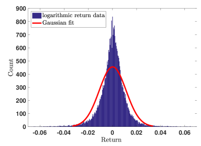
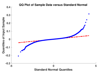
Figure 1: Histogram of daily Dow Jones data with a Gaussian fit (left hand side) and a quantile-quantile plot of the logarithmic return data. Dow Jones data (May 27, 1896-November 14, 2018). Source: https://stooq.com (accessed on November 15, 2018).

A further possibility for visualization of the fat-tail property of stock returns is to make use of quantile-quantile plots (qq-plots). The qq-plot in figure 1 plots the data against a Gaussian distributions and the deviations from the straight line clearly indicates the fat-tail behavior.

A further example of a stylized fact in stock prices is volatility clustering, obtained again by Mandelbrot (Mandelbrot 1997). This stylized fact can be quantified with the help of the auto-correlation function. Since the stock return distribution is assumed to be a stationary stochastic process one can calculate the correlation between stock returns at different points in time. The auto-correlation for the stationary stochastic process $R(t),\ t>0$ is given by:

$$C(l):=Corr(R(t+l),R(t))=\frac{Cov(R(t+l),R(t))}{E[(R(t)-\bar{R})^{2}]}=\frac{E[(R(t+l)-\bar{R})\ (R(t)-\bar{R})]}{E[(R(t)-\bar{R})^{2}]},\ l>0$$

The correlation $Corr$ is given by the normalized covariance $Cov$ of two random variables. The auto-correlation function $C(l)\in[-1,1]$ depends on the time shift called lag $l>0$ of the stochastic process. Empirical data reveals that raw returns are not auto-correlated but in fact absolute or quadratic raw returns possess significant auto-correlation. Interestingly, in the case of absolute or squared returns the auto-correlation function exhibits an algebraic decay similar to the stock return distribution.

$$Corr(|R(t+l)|,|R(t)|)\sim\frac{1}{l^{\beta}},\ \beta>0.$$

The Figure 2 depicts the empirical auto-correlation function of raw and absolute daily returns of DAX data. We clearly obtain no auto-correlation for raw returns and a slowly decreasing auto-correlation with respect to the time lag for absolute returns.

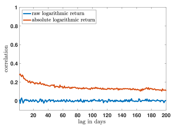
Figure 2: Auto-correlation of raw and absolute returns of daily Dow Jones data (May 27, 1896-November 14, 2018). Source: https://stooq.com (accessed on November 15th 2018).

Besides the previously presented stylized facts there are at least thirty stylized facts documented (Chen et al. 2012; Lux 2008). For a detailed discussion on stylized facts we refer to (Cont 2001; Ehrentreich 2007; Campbell et al. 1997; Pagan 1996; Lux 2008).

Although stylized facts are “almost universally accepted among economists and physicists” (Maldarella and Pareschi 2012), the origins of stylized facts remain widely undiscovered (Pagan 1996; Cowan and Jonard 2002; Maldarella and Pareschi 2012). For example many stylized facts cannot be explained by the famous Efficient Market Hypothesis by Eugene Fama (Fama 1965) which has been the dominant paradigm in macroeconomics for many years. Furthermore, several studies indicate that stylized facts play a crucial role in the creation of financial crashes (Farmer and Foley 2009; LeBaron 2006).

2.1 Empirical Data

The empirical results for the excess kurtosis, Hill estimator and auto-correlations for the daily logarithmic stock returns and absolute logarithmic stock returns of the indices DAX, Dow Jones and S&P have been computed. We review two data sources, namely Yahoo and Stooq. The Hill estimator is calculated on the upper 5% of the stock return data. The auto-correlation is evaluated for different time lags $(10,20,50,100)$. Furthermore, we consider different time horizons of our indices as presented in the Tables 1-5.

The data reveals that the excess kurtosis is very sensitive with respect to different indices. Thus, we obtain differences in the excess kurtosis of DAX and S&P data with a factor of more than four (see Table 1 ). In addition, these tables reveal that the time horizon has an impact on all other statistical quantities as well. For example one may compare Table 1 with Table 2 or Table 3 with Table 5. Finally, we aim to discuss the quality of the data. For all time horizons, where data of both sources were available, we presented them. The results indicate that the quality of the data appears sufficient. Differences are only obtained in an order of magnitude $10^{-2}$. Nevertheless, we have marked the largest differences (see Tables 2, 4).

	DAX 1959-2018	DAX 1980-2018	DJ 1896-2018	SP 1789-2018	SP 1980-2018
Skew	-0.15398	-0.29760	-0.53018	0.04980	-1.15998
Excess Kurtosis	7.48509	6.41534	19.94971	32.49845	26.80929
Hill 5%	2.86114	2.95151	2.61625	2.38089	2.87303
AutoCorr 10	0.00097	-0.00215	0.01552	0.00801	0.01431
AutoCorr 20	0.00993	0.01534	0.01043	0.00537	0.01499
AutoCorr 50	-0.00689	-0.00663	0.00169	-0.00973	-0.02552
AutoCorr 100	-0.00382	-0.00081	0.00866	0.00432	0.01582

Table 1: Market Data: Log returns from Stooqs daily open prices

	DAX		Dow Jones		S&P 500
	Stooqs	Yahoo	Stooqs	Yahoo	Stooqs	Yahoo
Hill 5%	3.27487	3.27484	2.36088	2.36088	2.25837	2.25842
Excess Kurtosis	5.85989	5.86956	10.9572	10.9333	11.1009	11.0984
Skew	0.00476301	-0.00979905	-0.0866539	-0.0858895	-0.340703	-0.340731
AutoCorr 10	0.0045713	0.0143741	0.0275151	0.0276896	0.0351904	0.0356558
AutoCorr 20	0.0133577	0.00854401	0.0557108	0.0547723	0.0614776	0.0606093
AutoCorr 50	-0.0677308	-0.0366783	-0.0473323	-0.0463268	-0.0573844	-0.0554321
AutoCorr 100	0.0224124	0.0131171	0.0128191	0.0126586	0.0227003	0.0222299

Table 2: Market Data: Log returns of open prices for 10 years (1/1/2008 - 1/1/2018) with about 2538 trading days. Large Deviations are highlighted.

	DAX		Dow Jones		S&P 500
	Stooqs	Yahoo	Stooqs	Yahoo	Stooqs	Yahoo
Hill 5%	3.12956	3.08732	2.77032	2.7728	2.506	2.50589
Excess Kurtosis	14.1932	14.1195	22.0448	22.0289	20.3362	20.3454
Skew	2.78073	2.78152	3.54775	3.54489	3.5181	3.5183
AutoCorr 10	0.206428	0.205136	0.322451	0.321833	0.334737	0.33453
AutoCorr 20	0.16254	0.172491	0.280044	0.2803	0.286463	0.286256
AutoCorr 50	0.0876169	0.0711959	0.173887	0.174129	0.180332	0.180348
AutoCorr 100	0.0771358	0.0793103	0.144337	0.143757	0.142684	0.142319

Table 3: Market Data: Abs log returns of open prices for 10 years (1/1/2008 - 1/1/2018) with about 2538 trading days.

	DAX		Dow Jones		S&P 500
	Stooqs	Yahoo	Stooqs	Yahoo	Stooqs	Yahoo
Hill 5%	3.0432	3.02615	2.72374	2.7234	2.56005	2.56067
Excess Kurtosis	4.11224	4.14143	7.96191	7.95903	8.08028	8.09152
Skew	-0.0936016	-0.0868356	-0.115667	-0.115951	-0.217571	-0.218462
AutoCorr 10	-0.0126055	-0.00218874	0.0221733	0.0222847	0.0236101	0.0237844
AutoCorr 20	0.0215986	0.0208578	0.0149777	0.0151891	0.0177763	0.0177882
AutoCorr 50	-0.0228001	-0.00978986	-0.0311535	-0.0310373	-0.0366033	-0.0360126
AutoCorr 100	0.0104454	0.00583078	0.020815	0.0209226	0.0235104	0.0232849

Table 4: Market Data: Log returns of open prices for 20 years (1/1/1998 - 1/1/2018) with about 5079 trading days. Large Deviations are highlighted.

	DAX		Dow Jones		S&P 500
	Stooqs	Yahoo	Stooqs	Yahoo	Stooqs	Yahoo
Hill 5%	3.30068	3.24861	2.95592	2.95606	2.95044	2.95047
Excess Kurtosis	9.64775	9.68247	18.3816	18.3859	17.5795	17.6036
Skew	2.36843	2.37762	3.10218	3.10216	3.08068	3.08304
AutoCorr 10	0.245037	0.248828	0.272268	0.27209	0.288187	0.288096
AutoCorr 20	0.201899	0.201428	0.227346	0.227286	0.236044	0.235682
AutoCorr 50	0.153015	0.145099	0.155416	0.155355	0.167528	0.167349
AutoCorr 100	0.118164	0.118089	0.117543	0.117262	0.121554	0.12127

Table 5: Market Data: Abs log returns of open prices for 20 years (1/1/1998 - 1/1/2018) with about 5079 trading days.

3 Agent-Based Models

One possible approach to gain insights into the creation of stylized facts are computational agent-based models which are part of the research field econophysics. This approach borrows tools from statistical mechanics, such as Monte-Carlo simulations, and are often inspired by physical theories or models such as kinetic theory or the famous Ising model. Agent-based modeling has become very popular modeling tool over the last decade (Farmer and Foley 2009; Hommes 2006; Tesfatsion 2002). Such model can be applied to nearly all fields of economics, examples include wealth formation, firm size, stock market, policy design, innovation change or auction markets. The starting point of the first modern multi-agent model (Samanidou et al. 2007) is probably the market crash of 20% at the US stock market in 1987. This extreme anomaly known as Black Monday, which economists failed to provide an explanation for, encouraged the economists Kim and Markowitz to design an agent-based model (Kim and Markowitz 1989). They tried to discover connections between agents who follow a portfolio insurance strategy and the volatility of the market with the help of Monte-Carlo simulations.

These modern financial market models of interacting heterogeneous agents share many similarities with interacting particle systems from physics (Sornette 2014; Zschischang and Lux 2001; Lux et al. 2008). These models usually consider bounded rational agents in the sense of Simon (Simon 1955) and are influenced by behavioral finance (LeBaron 2006; Farmer and Foley 2009; Hommes 2006; Chen et al. 2012). Many agent-based financial market models are able to replicate the most prominent stylized facts of financial markets such as fat-tails of asset returns or volatility clustering. Thus, these computational agent-based models are able to shed light on the origins of stylized facts. More precisely they are able to find sufficient conditions for the agent or market design in order to obtain stylized facts.

As many studies indicate behavioral aspects of financial agents may be one reason for the creation of stylized facts (Cross et al. 2005; Lux 2008; Chen et al. 2012). New theories have been developed such as the interacting agent hypothesis (Lux and Marchesi 1999; Ehrentreich 2007) or the heterogeneous market hypothesis proposed by Hommes (Hommes 2001; Ehrentreich 2007) as alternatives to the efficient market hypothesis. For a comprehensive introduction to agent-based models we refer to (Ehrentreich 2007; Chen et al. 2012; Janssen and Ostrom 2006; Cont 2007; LeBaron 2000, 2006; Samanidou et al. 2007; Hommes 2006; Iori et al. 2012; Sornette 2014).

The great advantage of agent-based models compared to traditional models is the possibility to design complex agents and study the interaction of those by computer simulations. As the name reveals, the modeling of the agent is the key aspect. Modeling financial agents has a long tradition in economics and dates back the work of Smith (Smith 1937). Recent developments in the field of behavioral finance had a significant influence on agent-based models. In the next paragraph, we will provide a short overview of agent modeling and introduce the concept of bounded rational agents which is used in most agent-based models.

Modeling Agents

The question of modeling financial agents is actually concerned with the modeling of a decision-making process. Thus, in the case of an financial market, agents are faced with the decision to buy, hold or sell a stock (good) or to be flat in the market. The theory of choice is known in economics as decision theory or utility theory. Besides early contributions of Bentham, Gossen and Depuit, modern utility theory has been developed by Walras and Menger (Stigler 1950). These early studies focused on proper utility measures and utility maximization. Notable contributions on the mathematization of utility models have been published by Edgeworth (Edgeworth 1881).
In the context of financial market models respectively agent-based models, we are especially interested in the theory of expected utility also known as expected utility hypothesis. This theory deals with the modeling of the decision process of persons under uncertain outcomes. The first example for the problem of choice under uncertainties was given by Bernoulli in 1713 with the famous St. Petersburg paradox. In the 1930s and 1940s, the expected utility hypothesis has been put on a solid mathematical foundation by the mathematician von Neumann and economist Morgenstern. In 1944, they published the famous von Neumann-Morgenstern utility theorem (Von Neumann et al. 2007) which precisely defines when a decision maker is rational, i.e. if a utility function and the corresponding maximum exist.
The model of rational expectation of financial agents has been rigorously defined by Muth in 1961 (Muth 1961) and is known as the rational expectation hypothesis. It says that the agents’ expectation (e.g. of the future stock price) is equal to the true expected value of the economic asset. Thus, the agents’ expectations may deviate from the correct value but is true on the average. This theory became the dominant macroeconomic approach after Lucas used it in his famous Lucas critique in 1976 (Lucas Jr 1976; Ehrentreich 2008). Furthermore, the rational expectation hypothesis is the foundation of the famous efficient market hypothesis by E. Fama (Malkiel and Fama 1970).
As discussed earlier, market models of rational agents are not able to explain and reproduce stylized facts. For that reason agent-based models do not follow the rational expectation hypothesis, they follow the ansatz of boundedly rational agents. Thus, also behavioral aspects are considered in the decision making of the agents.

Bounded Rational Agents

The concept of bounded rational agents has been introduced by Simon (Simon 1955, 1957). Like the theory of expected utility, this is a model of the agents’ choice. Bounded rational agents do not only act rational but partly irrational. Mathematically, they do not solve an optimization problem, but rather look for a satisfactory solution which is near the optimum. This can be supported by the fact that the computational resources, respectively the time to solve the optimization problem are limited in real world application (Ehrentreich 2008). Furthermore, it is well known that fund managers often prefer to apply heuristics than to solve a highly complex optimization problem. One extension of this model has been derived by Rubinstein (Rubinstein 1998). The concept of bounded rational agents is heavily influenced and supported by behavioral finance. Thus, the deviations of financial agents to the optimal solution can be accounted for behavioral biases of agents. Probably the most famous theory in behavioral finance is the so called prospect theory which has been established by Kahnemann and Tversky in their seminal paper Prospect Theory: An Analysis of Decision under Risk in 1979. Prospect theory deals with the decision making of agents under uncertain outcomes. It attempts to approximate real-life heuristics of decision makers which are influenced by psychological effects. In some sense, this theory can be seen as an extension of the expected utility theory.

3.1 Abstract Agent-Based Economic Market Model

We review the recently introduced abstract agent-based economic market (ABEM) model (Trimborn et al. 2019). The authors introduce a universal meta-model which helps to create, compare and categorize ABEM models. The core idea is to define building blocks which are universal for most ABEM models. These building blocks are agent design, market mechanism and environment. By agent design we mean the precise definition of an agent in each model. The market mechanism can be interpreted in the broadest sense as a rule which fixes a price of a good or stock at a financial market or between the agents. The last building block is the environment, which can be seen as an additional coupling or spatial correlation among agents. A schematic picture of this meta-model is given in Figure 3. In the following we will give specific examples of each building block. We dispense on a rigorous mathematical definition of each building block as done in (Trimborn et al. 2019).

Figure 3: Schematic picture of abstract ABEM model.

Price Adjustment

We aim to specify what we mean by price adjustment process. We define such a mechanism as a law which fixes a price of a certain good, stocks or bonds on a market. Such a market may consist of all agents or an interaction of a subset of all agents. Examples of a price adjustment process that considers all agents is a stock market which fixes the price for all agents. An example of a price process that only considers a subset of agents may be a binary trade between agents or an auction. Clearly, by this definition of a pricing process we implicitly define a financial agent as an actor on the market equipped with a personal supply or demand. Exemplified, we present a general disequilibrium market model implemented in many ABEM models (Trimborn et al. 2019).
We define the microscopic excess demand of all agents, given by demand minus supply. These microscopic excess demands $ed_{i},i=1,...,N$ of all agents can be aggregated to an aggregated excess demand $ED$.

$$ED:=\frac{1}{N}\sum\limits_{i=1}^{N}ed_{i}.$$

For a rigorous definition of aggregated excess demand we refer to (Mantel 1974; Debreu 1974; Sonnenschein 1972). A general disequilibrium market model build on the idea of Beja and Goldman (Beja and Goldman 1980) is given by:

$$S_{k+1}=S_{k}+F(S_{k},ED_{k})+G(S_{k},ED_{k})\ \eta,$$ (1)

Here, $\eta$ is a Gaussian distributed random variable and (1) is a difference equation. The index $k\in\mathbb{N}$ is the discretized time steps ($S_{k}=S(t+k\ \Delta t)$ for a fixed initial time $t$ and time step $\Delta t>0$). Furthermore, $F,G$ model arbitrary functions. Many price adjustment processes of ABEM models are special cases of model (1), for example the models presented in (Day and Huang 1990; Alfarano et al. 2008; Lux 1995; Chiarella et al. 2002, 2005, 2006, 2007; Challet et al. 2001; Zhou and Sornette 2007; Andersen and Sornette 2003; Harras and Sornette 2011; Sornette and Zhou 2006; Kaizoji et al. 2002; Palmer et al. 1994; Bouchaud and Cont 1998; Cont and Bouchaud 2000; Cross et al. 2005, 2007, 2006; Dieci et al. 2006; Farmer and Joshi 2002; Lux and Marchesi 1999, 2000; De Grauwe and Grimaldi 2005).

Agent Design

The agent design differs for each field of applications. Frequently used quantities which characterize the financial agent is wealth, investment propensity or agent’s excess demand. In the following we present examples of agent’s excess demand. Many ABEMM models such as (Chiarella et al. 2006; Beja and Goldman 1980; Hommes 2001, 2006; Lux 1995; Franke and Westerhoff 2009) only consider two agents.

Example 1.

Frequently used financial agents in ABEM models are fundamentalist and chartists (Lux 1998; Hommes 2006). A fundamental agent believes that to every stock or good there is a fair market price (or fundamental value) $P^{F}>0$ and that the market price will converge to this fundamental value. Hence, a fundamentalist wants to sell stocks if the stock price is above the fundamental value and he buys stocks if the market price is below the fundamental value. Hence the agent’s demand can be calculated as follows

$$ed^{F}(t_{k}):=a\ (P^{F}(t_{k})-P(t_{k})),$$

for a positive weight $a>0$ and a logarithmic stock price $P(t_{k})\in\mathbb{R}$ with the discretized time $t_{k}:=t_{0}+k\ \Delta t,\ \Delta t>0\ k\in\mathbb{N}$. Here, $t_{0}>0$ denotes the initial time. A chartist assumes that the future stock return is best approximated by extrapolating past returns. One simple example of such an investor is

$$ed^{C}(t_{k}):=b\ (P(t_{k})-P(t_{k-1})),$$

for a positive weight $b>0$. Examples of such agents can be found in the models (Chiarella et al. 2006; Beja and Goldman 1980; Hommes 2001, 2006; Lux 1995; Franke and Westerhoff 2009).

In the previous example we presented two possible excess demands of two financial agents. In the following we provide an example of how these excess demands can be aggregated into the aggregated excess demand.

Example 2.

A simple example is the Franke-Westerhoff model (Franke and Westerhoff 2009, 2011, 2012) where the population of agents is fully described by two agents ($N=2$), a chartist and a fundamentalist. Hence, the excess demand is defined as

$$ED^{FW}(t_{k})=\frac{1}{2}\left(ed^{FW}_{C}(t_{k})+ed^{FW}_{F}(t_{k})\right).$$

In comparison to the general chartist and fundamental demand defined in Example 1 the Franke-Westerhoff models considers time dependent weights $a,b$ and additionally there is a random variable added.

Then the price adjustment process as defined in the previous paragraph may utilize the aggregated excess demand in order to fix the price. Clearly the above ideas have been generalized for $N$ agent designs (Cross et al. 2005; Harras and Sornette 2011; Chen et al. 2012). Especially we aim to emphasize that the previous example does not nearly cover the full range of possible agent designs.

Environment

The previously introduced building blocks, agent design and price adjustment seem to be a natural structure in agent-based models. We aim to introduce the notion of environment which is to us the third building bock. This concept has been first introduced in (Trimborn et al. 2019) and needs to be explained.

An environment subsumes any additional coupling, besides of the coupling via the price adjustment process, between the agents. The most famous example possibly is herding, which is frequently used in ABEM models (Alfarano et al. 2005; Kirman et al. 2001; Kirman 1993; Cross et al. 2005; Franke and Westerhoff 2012). Further examples are any spatial structure e.g. a network structure of agents or any prioritization of special financial agents (Ausloos et al. 2015; Alfarano and Milaković 2009, 2008; Harras and Sornette 2011; Gurgone et al. 2018). As an example we aim to present the herding mechanism of the Cross model (Cross et al. 2005).

Example 3.

We define the herding mechanism of the Cross model (Cross et al. 2005). Each agent is described by a herding pressure $c_{i}>0$ and the evolution reads

$$\begin{cases}c_{i}(t+\Delta t)=c_{i}(t)+\Delta t|ED(t)|,&\text{if}\ \sigma_{i}(t)\ ED(t)<0\\ c_{i}(t+\Delta t)=c_{i}(t),&\text{otherwise}.\end{cases}$$

Thus, the herding pressure is increased if the investment decision of the agent $\sigma_{i}\in\{-1,1\}$ has the opposite sign as the aggregated excess demand $ED$. This situation corresponds to the fact that the agents’ position is in the minority. The agent switches position if the herding pressure $c_{i}$ has reached a threshold $\alpha_{i}>0$. After a switch the herding pressure gets reset to zero. This herding mechanism leads to additional coupling beneath the agents, introduced by the coupling with the aggregated excess demand.

Finally, we aim to stress that these environments seem to be crucial in the generation of stylized facts. This seems to be natural since such an additional coupling often models behavioral aspects of agents e.g. herding. This coupling often leads to additional correlations among agents which may lead to clustering phenomena.

4 Conclusion

In the first part we have given an overview of the most perceived stylized facts, namely fat-tails in asset returns, volatility clustering and absence of auto-correlation. Additionally, we have presented empirical results of DAX, Dow Jones and S&P data. We established that the excess kurtosis is a very volatile measure and heavily changes between different indices. Furthermore, we concluded that even the time horizon has an substantial impact on several statistical measures.

In the second part of the paper we have given an introduction to agent-based modeling. After a short literature study we presented a short historical overview and reported major developments in this field of research. Finally, we reviewed a recently introduced abstract ABEM model. This model subdivides ABEM models in three building blocks. Such an abstract formulation may help to create new models or compare existing ABEM models. A detailed categorization of known ABEM models in this abstract framework is left open for future research.

References

- Alfarano and Milaković (2008) Simone Alfarano and Mishael Milaković. Should network structure matter in agent-based finance? Technical report, Economics Working Paper, 2008.
- Alfarano and Milaković (2009) Simone Alfarano and Mishael Milaković. Network structure and n-dependence in agent-based herding models. Journal of Economic Dynamics and Control, 33(1):78–92, 2009.
- Alfarano et al. (2005) Simone Alfarano, Thomas Lux, and Friedrich Wagner. Estimation of agent-based models: the case of an asymmetric herding model. Computational Economics, 26(1):19–49, 2005.
- Alfarano et al. (2008) Simone Alfarano, Thomas Lux, and Friedrich Wagner. Time variation of higher moments in a financial market with heterogeneous agents: An analytical approach. Journal of Economic Dynamics and Control, 32(1):101–136, 2008.
- Andersen and Sornette (2003) J Vitting Andersen and Didier Sornette. The $-game. The European Physical Journal B-Condensed Matter and Complex Systems, 31(1):141–145, 2003.
- Ausloos et al. (2015) Marcel Ausloos, Herbert Dawid, and Ugo Merlone. Spatial interactions in agent-based modeling. In Complexity and Geographical Economics, pages 353–377. Springer, 2015.
- Beja and Goldman (1980) Avraham Beja and M Barry Goldman. On the dynamic behavior of prices in disequilibrium. The Journal of Finance, 35(2):235–248, 1980.
- Bouchaud and Cont (1998) J-P Bouchaud and Rama Cont. A langevin approach to stock market fluctuations and crashes. The European Physical Journal B-Condensed Matter and Complex Systems, 6(4):543–550, 1998.
- Brada et al. (1966) Josef Brada, Harry Ernst, and John Van Tassel. Letter to the editor—the distribution of stock price differences: Gaussian after all? Operations Research, 14(2):334–340, 1966.
- Campbell et al. (1997) John Y Campbell, Andrew Wen-Chuan Lo, Archie Craig MacKinlay, et al. The econometrics of financial markets, volume 2. princeton University press Princeton, NJ, 1997.
- Challet et al. (2001) Damien Challet, Matteo Marsili, and Yi-Cheng Zhang. Stylized facts of financial markets and market crashes in minority games. Physica A: Statistical Mechanics and its Applications, 294(3):514–524, 2001.
- Chen et al. (2012) Shu-Heng Chen, Chia-Ling Chang, and Ye-Rong Du. Agent-based economic models and econometrics. The Knowledge Engineering Review, 27(02):187–219, 2012.
- Chiarella et al. (2002) Carl Chiarella, Roberto Dieci, and Laura Gardini. Speculative behaviour and complex asset price dynamics: a global analysis. Journal of Economic Behavior & Organization, 49(2):173–197, 2002.
- Chiarella et al. (2005) Carl Chiarella, Roberto Dieci, and Laura Gardini. The dynamic interaction of speculation and diversification. Applied Mathematical Finance, 12(1):17–52, 2005.
- Chiarella et al. (2006) Carl Chiarella, Roberto Dieci, and Laura Gardini. Asset price and wealth dynamics in a financial market with heterogeneous agents. Journal of Economic Dynamics and Control, 30(9):1755–1786, 2006.
- Chiarella et al. (2007) Carl Chiarella, Roberto Dieci, and Xue-Zhong He. Heterogeneous expectations and speculative behavior in a dynamic multi-asset framework. Journal of Economic Behavior & Organization, 62(3):408–427, 2007.
- Cont (2001) Rama Cont. Empirical properties of asset returns: stylized facts and statistical issues. 2001.
- Cont (2007) Rama Cont. Volatility clustering in financial markets: empirical facts and agent-based models. In Long memory in economics, pages 289–309. Springer, 2007.
- Cont and Bouchaud (2000) Rama Cont and Jean-Philipe Bouchaud. Herd behavior and aggregate fluctuations in financial markets. Macroeconomic dynamics, 4(2):170–196, 2000.
- Cowan and Jonard (2002) Robin Cowan and Nicolas Jonard. Heterogenous agents, interactions and economic performance, volume 521. Springer Science & Business Media, 2002.
- Cross et al. (2005) Rod Cross, Michael Grinfeld, Harbir Lamba, and Tim Seaman. A threshold model of investor psychology. Physica A: Statistical Mechanics and its Applications, 354:463–478, 2005.
- Cross et al. (2006) Rod Cross, Michael Grinfeld, and Harbir Lamba. A mean-field model of investor behaviour. In Phys.: Conf. Series, volume 55, pages 55–62, 2006.
- Cross et al. (2007) Rod Cross, Michael Grinfeld, Harbir Lamba, and Tim Seaman. Stylized facts from a threshold-based heterogeneous agent model. The European Physical Journal B, 57(2):213–218, 2007.
- Day and Huang (1990) Richard H Day and Weihong Huang. Bulls, bears and market sheep. Journal of Economic Behavior & Organization, 14(3):299–329, 1990.
- De Grauwe and Grimaldi (2005) Paul De Grauwe and Marianna Grimaldi. Heterogeneity of agents, transactions costs and the exchange rate. Journal of Economic Dynamics and Control, 29(4):691–719, 2005.
- Debreu (1974) Gerard Debreu. Excess demand functions. Journal of mathematical economics, 1(1):15–21, 1974.
- Dieci et al. (2006) Roberto Dieci, Ilaria Foroni, Laura Gardini, and Xue-Zhong He. Market mood, adaptive beliefs and asset price dynamics. Chaos, Solitons & Fractals, 29(3):520–534, 2006.
- Edgeworth (1881) Francis Ysidro Edgeworth. Mathematical psychics: An essay on the application of mathematics to the moral sciences, volume 10. Kegan Paul, 1881.
- Ehrentreich (2008) N Ehrentreich. Agent-based modeling: The santa fe institute artificial stock market, 2008.
- Ehrentreich (2007) Norman Ehrentreich. Agent-based modeling: The Santa Fe Institute artificial stock market model revisited, volume 602. Springer Science & Business Media, 2007.
- Eugene (1963) Fama Eugene. The distrigbution of the daily differences of the logarithms of stock prices. In Ph.D. Thesis. Graduate School of Business University of Chicago, 1963.
- Fama (1965) Eugene F Fama. The behavior of stock-market prices. The journal of Business, 38(1):34–105, 1965.
- Farmer and Foley (2009) J Doyne Farmer and Duncan Foley. The economy needs agent-based modelling. Nature, 460(7256):685–686, 2009.
- Farmer and Joshi (2002) J Doyne Farmer and Shareen Joshi. The price dynamics of common trading strategies. Journal of Economic Behavior & Organization, 49(2):149–171, 2002.
- Franke and Westerhoff (2009) Reiner Franke and Frank Westerhoff. Validation of a structural stochastic volatility model of asset pricing. Christian-Albrechts-Universität zu Kiel. Department of Economics, 2009.
- Franke and Westerhoff (2011) Reiner Franke and Frank Westerhoff. Estimation of a structural stochastic volatility model of asset pricing. Computational Economics, 38(1):53–83, 2011.
- Franke and Westerhoff (2012) Reiner Franke and Frank Westerhoff. Structural stochastic volatility in asset pricing dynamics: Estimation and model contest. Journal of Economic Dynamics and Control, 36(8):1193–1211, 2012.
- Gurgone et al. (2018) Andrea Gurgone, Giulia Iori, and Saqib Jafarey. The effects of interbank networks on efficiency and stability in a macroeconomic agent-based model. Journal of Economic Dynamics and Control, 91:257–288, 2018.
- Harras and Sornette (2011) Georges Harras and Didier Sornette. How to grow a bubble: A model of myopic adapting agents. Journal of Economic Behavior & Organization, 80(1):137–152, 2011.
- Hill (1975) Bruce M Hill. A simple general approach to inference about the tail of a distribution. The annals of statistics, pages 1163–1174, 1975.
- Hommes (2006) Cars H Hommes. Heterogeneous agent models in economics and finance. Handbook of computational economics, 2:1109–1186, 2006.
- Hommes (2001) Carsien Harm Hommes. Financial markets as nonlinear adaptive evolutionary systems. 2001.
- Iori et al. (2012) Giulia Iori, James Porter, et al. Agent-based modelling for financial markets. Chapter prepared for the Handbook on Computational Economics and Finance, 2012.
- Janssen and Ostrom (2006) Marco A Janssen and Elinor Ostrom. Empirically based, agent-based models. Ecology and society, 11(2), 2006.
- Kaizoji et al. (2002) Taisei Kaizoji, Stefan Bornholdt, and Yoshi Fujiwara. Dynamics of price and trading volume in a spin model of stock markets with heterogeneous agents. Physica A: Statistical Mechanics and its Applications, 316(1):441–452, 2002.
- Kim and Markowitz (1989) Gew-rae Kim and Harry M Markowitz. Investment rules, margin, and market volatility. The Journal of Portfolio Management, 16(1):45–52, 1989.
- Kirman (1993) Alan Kirman. Ants, rationality, and recruitment. The Quarterly Journal of Economics, 108(1):137–156, 1993.
- Kirman et al. (2001) Alan P Kirman, Gilles Teyssiere, et al. Microeconomic models for long-memory in the volatility of financial time series. Technical report, Society for Computational Economics, 2001.
- LeBaron (2000) Blake LeBaron. Agent-based computational finance: Suggested readings and early research. Journal of Economic Dynamics and Control, 24(5):679–702, 2000.
- LeBaron (2006) Blake LeBaron. Agent-based financial markets: Matching stylized facts with style. Post Walrasian Macroeconomics: Beyond the DSGE Model, pages 221–235, 2006.
- Lucas Jr (1976) Robert E Lucas Jr. Econometric policy evaluation: A critique. In Carnegie-Rochester conference series on public policy, volume 1, pages 19–46. North-Holland, 1976.
- Lux (1995) Thomas Lux. Herd behaviour, bubbles and crashes. The economic journal, pages 881–896, 1995.
- Lux (1998) Thomas Lux. The socio-economic dynamics of speculative markets: interacting agents, chaos, and the fat tails of return distributions. Journal of Economic Behavior & Organization, 33(2):143–165, 1998.
- Lux (2008) Thomas Lux. Stochastic behavioral asset pricing models and the stylized facts. Technical report, Economics working paper/Christian-Albrechts-Universität Kiel, Department of Economics, 2008.
- Lux and Marchesi (1999) Thomas Lux and Michele Marchesi. Scaling and criticality in a stochastic multi-agent model of a financial market. Nature, 397(6719):498–500, 1999.
- Lux and Marchesi (2000) Thomas Lux and Michele Marchesi. Volatility clustering in financial markets: a microsimulation of interacting agents. International journal of theoretical and applied finance, 3(04):675–702, 2000.
- Lux et al. (2008) Thomas Lux et al. Applications of statistical physics in finance and economics. Technical report, Kiel working paper, 2008.
- Maldarella and Pareschi (2012) Dario Maldarella and Lorenzo Pareschi. Kinetic models for socio-economic dynamics of speculative markets. Physica A: Statistical Mechanics and its Applications, 391(3):715–730, 2012.
- Malkiel and Fama (1970) Burton G Malkiel and Eugene F Fama. Efficient capital markets: A review of theory and empirical work. The journal of Finance, 25(2):383–417, 1970.
- Mandelbrot (1997) Benoit B Mandelbrot. The variation of certain speculative prices. In Fractals and scaling in finance, pages 371–418. Springer, 1997.
- Mantel (1974) Rolf R Mantel. On the characterization of aggregate excess demand. Journal of economic theory, 7(3):348–353, 1974.
- Muth (1961) John F Muth. Rational expectations and the theory of price movements. Econometrica: Journal of the Econometric Society, pages 315–335, 1961.
- Pagan (1996) Adrian Pagan. The econometrics of financial markets. Journal of empirical finance, 3(1):15–102, 1996.
- Palmer et al. (1994) Richard G Palmer, W Brian Arthur, John H Holland, Blake LeBaron, and Paul Tayler. Artificial economic life: a simple model of a stockmarket. Physica D: Nonlinear Phenomena, 75(1-3):264–274, 1994.
- Pareto (1897) Vilfredo Pareto. Cours d’économie politique, professé à l’université de lausanne. tome second, 1897.
- Rubinstein (1998) Ariel Rubinstein. Modeling bounded rationality. MIT press, 1998.
- Samanidou et al. (2007) Egle Samanidou, Elmar Zschischang, Dietrich Stauffer, and Thomas Lux. Agent-based models of financial markets. Reports on Progress in Physics, 70(3):409, 2007.
- Simon (1955) Herbert A Simon. A behavioral model of rational choice. The quarterly journal of economics, pages 99–118, 1955.
- Simon (1957) Herbert A Simon. Models of man; social and rational. 1957.
- Smith (1937) Adam Smith. The wealth of nations [1776], 1937.
- Sonnenschein (1972) Hugo Sonnenschein. Market excess demand functions. Econometrica: Journal of the Econometric Society, pages 549–563, 1972.
- Sornette (2014) Didier Sornette. Physics and financial economics (1776–2014): puzzles, ising and agent-based models. Reports on Progress in Physics, 77(6):062001, 2014.
- Sornette and Zhou (2006) Didier Sornette and Wei-Xing Zhou. Importance of positive feedbacks and overconfidence in a self-fulfilling ising model of financial markets. Physica A: Statistical Mechanics and its Applications, 370(2):704–726, 2006.
- Stigler (1950) George J Stigler. The development of utility theory. i. Journal of political economy, 58(4):307–327, 1950.
- Tesfatsion (2002) Leigh Tesfatsion. Agent-based computational economics: Growing economies from the bottom up. Artificial life, 8(1):55–82, 2002.
- Trimborn et al. (2019) Torsten Trimborn, Philipp Otte, Simon Cramer, Max Beikirch, Emma Pabich, and Martin Frank. Sabcemm-a simulator for agent-based computational economic market models. Computational Economics, 2019.
- Von Neumann et al. (2007) John Von Neumann, Oskar Morgenstern, and Harold William Kuhn. Theory of games and economic behavior (commemorative edition). Princeton university press, 2007.
- Zhou and Sornette (2007) W-X Zhou and Didier Sornette. Self-organizing ising model of financial markets. The European Physical Journal B, 55(2):175–181, 2007.
- Zschischang and Lux (2001) Elmar Zschischang and Thomas Lux. Some new results on the levy, levy and solomon microscopic stock market model. Physica A: Statistical Mechanics and its Applications, 291(1):563–573, 2001.