Multi-Modal Deep Clustering: Unsupervised Partitioning of Images

Abstract

The clustering of unlabeled raw images is a daunting task, which has recently been approached with some success by deep learning methods. Here we propose an unsupervised clustering framework, which learns a deep neural network in an end-to-end fashion, providing direct cluster assignments of images without additional processing. Multi-Modal Deep Clustering (MMDC), trains a deep network to align its image embeddings with target points sampled from a Gaussian Mixture Model distribution. The cluster assignments are then determined by mixture component association of image embeddings. Simultaneously, the same deep network is trained to solve an additional self-supervised task of predicting image rotations. This pushes the network to learn more meaningful image representations that facilitate a better clustering. Experimental results show that MMDC achieves or exceeds state-of-the-art performance on six challenging benchmarks. On natural image datasets we improve on previous results with significant margins of up to 20% absolute accuracy points, yielding an accuracy of 82% on CIFAR-10, 45% on CIFAR-100 and 69% on STL-10.

I Introduction

Clustering involves the organization of data in an unsupervised manner, based on the distribution of datapoints and the distances between them. Since these properties are closely tied to the representation of the data, the problems of clustering and data representation are firmly connected and are therefore sometimes solved jointly. In accordance, in this work we start from a recent method for the unsupervised computation of effective data representation (or features discovery), and develop a clustering method whose results significantly improve the state of the art in the clustering of natural images. The method is illustrated in Fig 1.

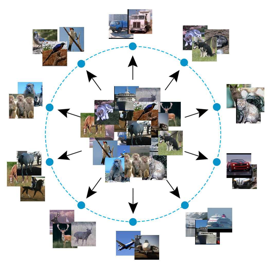
Figure 1: Our algorithm partitions a set of images into $k$ clusters by aligning image embeddings with target points sampled from a Gaussian Mixture Model on the $k$-dimensional unit sphere.

The task of unsupervised image clustering is challenging and interesting, as the algorithm needs to discover patterns in highly entangled data, and produce separated groups without explicitly specifying the grouping features. A large body of work has been devoted to the problem of clustering [20], see Section II for a brief review of some recent related work. In recent years, with the emergence of deep learning as the method of choice in visual object recognition and image classification, emphasis has shifted to the computation of effective representations that will support successful clustering [30]. Vice versa, unsupervised clustering loss has been used to drive the computation of image representation and the discovery of enhanced image features by making it possible to use unsupervised data in the training of deep networks, which traditionally require massive amounts of labeled data.

When learning feature representation from unsupervised data by minimizing a clustering-based loss function, one danger is cluster collapse - the representation may collapse to the trivial solution of a single cluster. In [3], a similar problem of representation collapse is managed by mapping the network’s representation to a fixed set of randomly chosen points in some target features space. Here we borrow this mapping idea, and incorporate it into a clustering algorithm.

More specifically, we first sample a fixed set of points in some target space. Since our method is designed to partition the data into $k$ clusters, the target points are chosen from a matched density function - Gaussian Mixture Model (GMM) with $k$ components. Our model trains a randomly initialized neural network to align its image embeddings with the sampled target points, directly inducing a partition that is based on the mixture components. This is done by simultaneously learning a one-to-one mapping between the output of the network and the target points, and updating the networks parameters to best fit images with their target points as assigned by the mapping.

In the absence of ground truth, the proposed approach is prone to instability as target points are continuously reassigned between images, creating a non-stationary online learning environment. Such instability is often linked with unsupervised learning tasks. To alleviate this problem, unsupervised tasks such as representation learning may be combined with self-supervision tasks to achieve better results [10]. Here we adopt the approach taken by [6] to deal with the notorious instability of training generative adversarial networks. Thus the model is jointly trained on the main clustering task and on a self-supervised auxiliary task as defined in RotNet [14], where all images are subjected to 4 rotation angles. In this auxiliary task the network is trained to recognize the $2D$ rotation of each rotated image.

For computation engine, our method uses off the shelf ConvNets and standard SGD training with mini-batch sampling in an end-to-end fashion. It is therefore scalable to large datasets. We evaluate our method on several standard benchmarks in image clustering, which is the goal of our method, significantly exceeding the state of the art on the 5 natural image datasets.

The rest of the paper is organized as follows: In Section II we briefly review recent related work. In Section III we describe our method in detail and elaborate on its various ingredients. Experimental results are reported in Section IV.

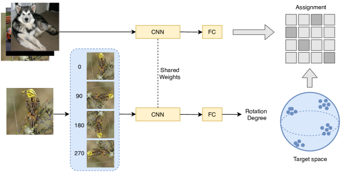
Figure 2: Our approach takes a set of images and solves two tasks in alternating epochs. In the primary task, a CNN is trained to produce output which matches some predefined set of target points sampled from a Gaussian mixture model, and optimally aligned with the training set. In the secondary task, given a rotated image, the same CNN is trained to predict the rotation angle of the image.

II Related work

Data clustering. The objective of data clustering is to partition data points into groups such that points in each group are more similar to each other than to data points in the other groups. Traditionally, clustering methods have been divided into density-based methods [24], partition-based methods [12], and hierarchical methods [11]. Partition-based methods, such as the popular k-means [32, 1], minimize a given clustering criterion by iteratively relocating data points between clusters until a (locally) optimal partition is attained. Density-based methods define clusters as areas with high density of points, separated by areas with low density of points [37]. Hierarchical based methods build a hierarchy of clusters in a top-to-bottom [34] or bottom-to-top [16] manner to determine clustering.

Representation Learning. Naïvely attempting to cluster images with traditional approaches does not produce a pleasing partitions of the images, as they work on the raw representations of the images in pixel space, whereas semantically similar images are not necessarily similar in the high-dimensional pixel space in which the images reside. In recent years learning useful image representations in an unsupervised manner has been dominated by deep-learning-based approaches. Autoencoders (AEs) [2] encode images with a deep network and are trained by reconstructing the image using a decoder network. These include several variations such as sparse AEs, denoising AEs [36], and more [29, 41]. Generative models such as Generative Adversarial Networks (GAN) [15] and variational autoencoders (VAE) [22] learn representations as a byproduct of learning to generate images. Tightly connected to our work, Noise-As-Targets (NAT) [3] and DeepCluster [4] adopt a training strategy of iteratively reassigning psuedo-labels to points while training the network to fit them (see Section III).

Self-supervised learning. A family of unsupervised learning algorithms that gained popularity in recent years are self-supervised methods. They learn representations by training a deep network to solve a pretext task, where labels can be produced directly from the data. Such tasks can be jigsaw puzzle solving [31], predicting the relative position of patches in an image [9], generating image regions conditioned on their surroundings [33], or more recently predicting image rotations (RotNet) [14]. In self-supervised GANs [6], predicting image rotations is used as an auxiliary task to stabilize and improve training, by enhancing the discriminator’s representation capabilities. Here we adopt this approach as well, as elaborated later on.

Deep clustering. The dominant and most successful approach to clustering of images in recent years has been to incorporate the tasks of representation learning and clustering into a single framework. Prominent works in the past years have been Joint Unsupervised Learning (JULE) [40], where the authors adopt an agglomerative clustering approach by iteratively merging clusters of deep representations and updating the networks parameters. Deep Adaptive Clustering (DAC) [5] recasts the clustering problem into a binary pairwise-classification framework, where cosine distances between image features of image pairs are used as a similarity measure to decide if they belong to the same cluster. Associative Deep Clustering (ADC) [17] jointly learns network parameters and embedding centroids with an association loss in order to estimate cluster membership. More recently, Invariant Information Clustering (IIC) [21] adopts an approach that achieves clustering based on maximizing the mutual information between two sets: deep embeddings of images, and instances of the images that underwent random image transformations while keeping the image semantic meaning intact. IIC leverages auxiliary over-clustering to increase expressivity in the learned feature representation, improving the representation capabilities of its network. This tactic bears resemblance to our incorporation of rotation prediction as an auxiliary task.

III Method

Our goal is to partition a set of images into $k$ clusters, which reflect internal structure in the data. Fig. 2 shows an overview of the proposed approach. The algorithm alternates between solving the main unsupervised clustering task, and an auxiliary self-supervised task that helps the training process. The ingredients of the method are described next. The full method is summarized in Algorithm 1.

III-A Unsupervised learning

The starting point for this work is an unsupervised learning framework for learning image representation from unlabeled data. The method, Noise as Targets [3], learns useful representations of images by training a deep network to align its images’ embeddings with a fixed set of target points. The target points are uniformly scattered on the $d$-dimensional unit sphere.

More specifically, let $X=\{x_{i}\}_{i=1}^{n}$ denote a set of images, and $f_{\theta}:X\rightarrow Z$ the parameterized deep network we wish to train. The output of $f_{\theta}$ is normalized to have $\ell_{2}$ norm of $1$, entailing that $Z$ is the $d$-dimensional unit sphere. NAT starts by uniformly sampling $n$ targets on this unit sphere. Let $\{t_{i}\}_{i=1}^{n}$ denote the set of target points, which remain fixed throughout the training. Each image $x_{i}$ is assigned a unique target $y_{i}$ through a permutation $P:[n]\rightarrow[n]$. The optimization objective is formulated as

$$\min\limits_{\theta,P}\frac{1}{n}\sum_{i}\ell(f_{\theta}(x_{i}),y_{i})~{}~{}~{}~{}~{}~{}y_{i}=t_{P(i)}$$ (1)

where $\ell$ is the Euclidean distance.

This optimization problem is solved in a stochastic manner, by iteratively solving it over randomly sampled mini-batches. Given a mini-batch of images $X_{b}$, the current representation vectors $f_{\theta}(X_{b})$ are first computed. Subsequently, Equation (1) is optimized for $P$ over the points in mini-batch $X_{b}$ using the Hungarian method [26], which reassigns the currently assigned targets of the mini-batch to minimize the Euclidean distance ($\ell_{2}$) between images and their assigned target points. Finally, the gradients of $f_{\theta}$ on $X_{b}$ with respect to $\theta$ are computed, and an SGD step is executed.

Intuitively, NAT permutes the assignment of image representation vectors to target points delivered by $f_{\theta}$, so that nearby embedding vectors are mapped to nearby target vectors, and then updates $\theta$ accordingly. This process leads to the grouping of semantically similar images in target space, and to effective representations that perform well in downstream computer vision classification and detection tasks.

  Input:
$\{x_{i}\}^{n}_{i=1}$ - images
$f_{\theta}$ - ConvNet with two heads
$k$ - number of clusters
$epochs$ - number of epochs to train
$iters$ - number of iterations in an epoch
$\sigma$ - variance of normal distribution
$d$ - dimension of embedding space
$\lambda_{c},\lambda_{r}$ - learning rates
$g$ - random image transformation
$r$ - number of instances of $g$ in a batch

  Init:
$P\leftarrow$ initialize with random assignments

$\theta\leftarrow$ initialize with random weights

$T\leftarrow$ initialize empty list

  for $i=1...n$ do

     sample $c\sim Categ(\frac{1}{K},...,\frac{1}{K})$

     sample $u\sim N(\mu_{c},\sigma\cdot I_{d\times d})$

     $T[i]\leftarrow t_{i}=\frac{u}{\|u\|}$

  end for

  for $e=1...epochs$ do

     for $i=1...iters$ do

        sample batch $X_{b}$ and assigned targets $T_{b}$

        compute $f_{\theta}(X_{b})$

        update $P$ by minimizing Equation (1) w.r.t $P$

        compute $\nabla_{\theta}L_{c}(\theta)$ of Equation (1) for $g(X_{b})$

        update $\theta\leftarrow\theta-\lambda_{c}\nabla_{\theta}L_{c}(\theta)$

     end for

     for $i=1...iters$ do

        sample batch $X_{b}$

        rotate $X_{b}$ $\forall r\in\{0^{\degree},90^{\degree},180^{\degree},270^{\degree}\}$

        compute $\nabla_{\theta}L_{r}(\theta)$ // $L_{r}$ is cross-entropy loss

        update $\theta\leftarrow\theta-\lambda_{r}\nabla_{\theta}L_{r}(\theta)$

     end for

  end for

Algorithm 1

III-B Multi-modal distribution of target points

The uniform distribution of target points on the unit sphere, as described above, is not well suited for unsupervised clustering, since it is likely to blur the dividing lines between clusters rather than sharpen them. Instead, multi-modal distribution seems like a natural choice for the objective of clustering, as it directly produces separated groups in target space.

In this work, we propose to use the mixture of Gaussians distribution, projected to the unit sphere, for the sampling of target points. Formally, this implies:

$$\begin{split}p(u)&=\sum^{K}_{k=1}\alpha_{k}\cdot p_{k}(u)~{}~{}~{}~{}~{}~{}~{}~{}~{}~{}~{}~{}u\in{\mathbb{R}}^{d}\\ p(t_{i})&=\int_{\frac{u}{\|u\|_{2}}=t_{i}}p(u)du~{}~{}~{}~{}~{}~{}~{}~{}~{}t_{i}\in Z\end{split}$$ (2)

where $K$ denotes the number of Gaussians in the mixture, $d$ the dimension of the embedding space, $\alpha_{k=1..K}$ a categorical random variable, and $p_{k}(u)$ the multivariate normal distribution $N(\mu_{k},\Sigma_{k})$, parameterized by mean vector $\mu_{k}$ and covariance matrix $\Sigma_{k}$. In the absence of prior knowledge we assume that the mixture components are equally likely, namely $\alpha_{k}=\frac{1}{K}\forall k\in[K]$. Finally, since the target points are constrained to lie on the unit sphere, we project the sample in $\mathbb{R}^{d}$ to the unit sphere by $t_{i}=\frac{u}{\|u\|_{2}}$.

We define the cluster assignment $c_{i}$ of image $x_{i}$ as follows

$$c_{i}=\operatorname*{arg\,min}\limits_{k}\|f_{\theta}(x_{i})-\mu_{k}\|_{2}$$ (3)

Note that if the final network $f_{\theta}$ fits that target points exactly, namely $f_{\theta}(x_{i})=y_{i}$, and if $\Sigma_{k}$ are the same $\forall k$, then with high probability $c_{i}$ is the index of the mixture component from which target point $y_{i}$ has been sampled.

III-C Image Transformations

Data augmentation is a useful and common technique to improve performance of machine learning algorithms. Usually, random image transformations such as cropping, flipping, rotation, scaling and photometric transformations are applied to images in order to expand the dataset with new and unique images. In our task of unsupervised clustering, these random transformations are essential, because they provide several instances of the same image that appear different but share the same semantic meaning as they contain the same object. Let $g$ denote a random image transformation. In our method, we use the center crop of an image when minimizing Equation (1) w.r.t $P$. When minimizing the same equation w.r.t $\theta$, we first apply $g$ to the image. Why is this algorithmic ingredient useful? When training the ConvNet, it must find common patterns between the original images and transformed images when fitting them to the same target. These common patterns are likely to appear in other images in the dataset belonging to the same class. This pushes the network to map images that contain the same objects closer to each other, in a similar manner to the beneficial effect of self-supervision.

TABLE I: Unsupervised clustering results. The results of our method are shown below the separation line. For each dataset, we show the average result over five runs, standard error (ste) and the best run. Above the separation line we list state of the art results for comparison, see review in Section II. Unreported results are marked with (-).

		MNIST		CIFAR-10		CIFAR-100		STL-10		ImageNet-10		Tiny-ImageNet
		NMI	ACC	NMI	ACC	NMI	ACC	NMI	ACC	NMI	ACC	NMI	ACC
k-means		0.499	0.572	0.087	0.228	0.083	0.129	0.124	0.192	0.119	0.241	0.065	0.025
SC		0.663	0.696	0.103	0.247	0.090	0.136	0.098	0.159	0.151	0.274	0.063	0.022
AE		0.725	0.812	0.239	0.313	0.100	0.164	0.249	0.303	0.210	0.317	0.131	0.041
DEC (2016)		0.772	0.843	0.257	0.301	0.136	0.185	0.276	0.359	0.282	0.381	0.115	0.037
JULE (2016)		0.913	0.964	0.192	0.272	0.103	0.137	0.182	0.277	0.175	0.300	0.102	0.033
DAC (2017)		0.935	0.978	0.396	0.522	0.185	0.238	0.249	0.303	0.394	0.527	0.190	0.066
IIC (2019)		0.978	0.992	0.513	0.617	0.224	0.257	0.431	0.4991	-	-	-	-
DCCM (2019)		-	-	0.496	0.623	0.285	0.327	0.376	0.482	0.608	0.710	0.224	0.108
Ours	avg.	0.971	0.990	0.703	0.820	0.418	0.446	0.593	0.694	0.719	0.811	0.274	0.119
	ste	$\pm$.000	$\pm$.000	$\pm$.011	$\pm$.019	$\pm$.003	$\pm$.006	$\pm$.005	$\pm$.013	$\pm$.008	$\pm$.012	$\pm$.001	$\pm$.001
	best	0.973	0.991	0.720	0.843	0.423	0.464	0.609	0.741	0.732	0.830	0.277	0.121

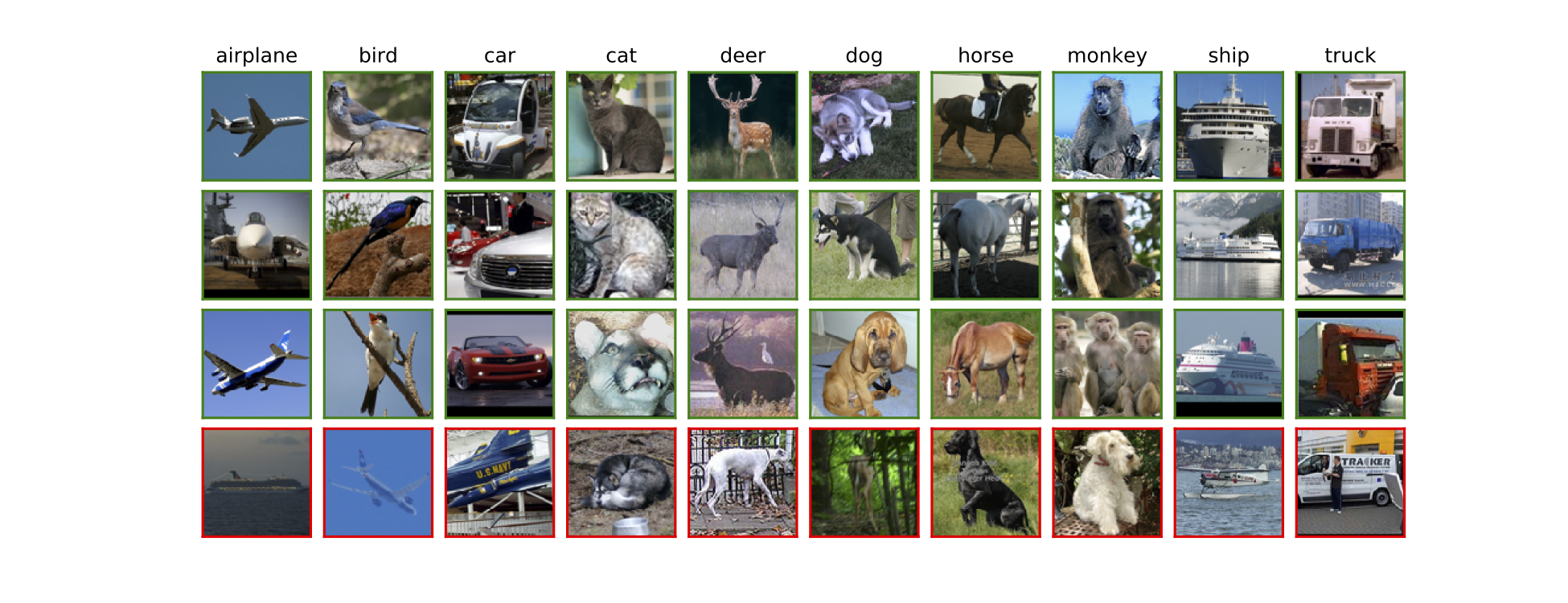
Figure 3: Unsupervised image clustering results on STL-10. Each column shows images from a different cluster. The top three images in each column are examples of images from the same class successfully clustered together. The images in the fourth row illustrate failure cases, where the image is assigned to the wrong cluster (e.g., an airplane assigned to the ’bird’ cluster).

III-D Auxiliary task

While optimizing the clustering objective (1), the ConvNet model simultaneously learns image representation and partitions the images. The success of unsupervised clustering is highly correlated with the quality of the learnt representation. It has been repeatedly shown that self-supervision methods can significantly improve the quality of representations in an unsupervised learning scenario. To benefit from this idea, we employ RotNet [14], which is a self-supervised learning algorithm that learns image features by training a ConvNet to predict image rotations. Specifically, images are rotated by $r$ degrees where $r\in\{0^{\degree},90^{\degree},180^{\degree},270^{\degree}\}$, and the model is subsequently trained to predict their rotation by optimizing the cross-entropy loss. RotNet produces competitive performance in representation learning benchmarks, and has been shown to benefit training in other tasks, when incorporated into a model as an auxiliary task [6, 13, 28]. We incorporate RotNet into our method, modifying the ConvNet training procedure to alternate between optimizing the main clustering task and this secondary auxiliary task.

III-E Refinement Stage

As we have no prior knowledge regarding the size of the clusters, we begin by assuming that clusters’ sizes are equal. When this assumption cannot be justified, we propose to augment the algorithm with an additional step, performed after the main training is concluded. In this step the assumption is relaxed, while target points are iteratively reassigned based on the outcome of k-means applied to $f_{\theta}(x_{1}),...,f_{\theta}(x_{n})$, and assigning image $x_{i}$ to target $\mu_{j}$ with label $j\in[K]$ derived from the outcome of k-means. This ingredient is similar to DeepCluster [4], proposed by Caron et al. as an approach for representation learning, where they perform the clustering on the latent vectors of the model and not the final output layer. A possible alternative method may start with this stage and discard the first one altogether, as this approach makes no assumption on the size of the clusters. However, we found that starting off with reassigning labels based on k-means is not competitive and produces less accurate clusters. For example, training on MNIST results in low accuracy of $81\%$ ($\pm 2.67$).

IV Experiments

We tested our method on several image datasets that are commonly used as benchmark for clustering, see results in Table I. We compare ourselves to state-of-the-art methods such as DEC [39], JULE [40], DAC [5], IIC [21] and DCCM [38]. In almost all cases our method improves on previous results significantly. Examples of clustering results on the STL-10 dataset of natural images are shown in Figure 3.

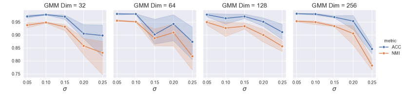
Figure 4: Comparison of clustering performance on MNIST with different Mixture of Gaussians initializations. We compare different dimensions for the target vectors and different coefficient parameters ($\sigma$) for the covariance matrices of the gaussians. These results do not include performing the refinement stage.

In the rest of this section we specify the implementation details of our method, and analyze the results. Subsequently, we report the results of an ablation study evaluating the various ingredients of the algorithm, which demonstrate how they contribute to its success. Our code is available online.

IV-A Implementation details and evaluation scores

Datasets. Six datasets are used in our empirical study: MNIST [27], CIFAR-10 [25], the 20 superclasses of CIFAR-100 [25], STL-10 [7], ImageNet-10 (a subset of ImageNet [8]) and Tiny-ImageNet [8], see Table II. We are most interested in the datasets that consist of natural images. These datasets are commonly used to evaluate clustering methods.

TABLE II: The image datasets used in our experiments.

Name	Classes	Samples	Dimension
MNIST	10	70,000	28$\times$28
CIFAR-10	10	60,000	32$\times$32$\times$3
CIFAR-100	20	60,000	32$\times$32$\times$3
STL-10	10	13,000	96$\times$96$\times$3
ImageNet-10	10	13,000	96$\times$96$\times$3
Tiny-ImageNet	200	100,000	64$\times$64$\times$3

Architectures. For the MNIST experiments we use a small VGG model [35] with batch normalization [19]. Each block in this neural network consists of one convolution layer, followed by a batch normalization layer and ReLU activation function, and ends with a max pooling layer. Our model has four blocks. For all other experiments we use a ResNet model [18] with 18 layers. These base models are followed by a linear prediction layer, that outputs the cluster assignments. When trained on the auxiliary task, the base model is also followed by another linear head, which predicts the image rotation.

Training details. The network is trained with stochastic gradient descent with learning rate $0.05$ and momentum of $0.9$. We apply weight decay of $0.0001$ for CIFAR-100 and Tiny-ImageNet, and $0.0005$ for all other datasets. We use batch size $128$ and perform random image augmentations which include cropping, flipping and color jitter. When training on the auxiliary rotation task, we rotate each image to all four orientations, resulting in an effective batch size of $512$. We train the network for $400$ epochs and decay learning rate by a factor of $5$ after $350$ epochs. For MNIST we train for $50$ epochs and decay learning rate by a factor of $10$ after $40$ epochs. Training on CIFAR-10 takes 10.5 hours on a single GTX-1080 GPU.

Mixture of Gaussians. We examined several initialization heuristics to determine the Gaussian means $\{\mu_{k}\}$ in the GMM distribution defined in (2) and the covariance matrices $\{\Sigma_{k}\}$. A comparison of different initialization schemes is provided in Figure 4, where all vectors lie on the $d$-dimensional unit sphere. Gaussian means $\{\mu_{k}\}$ are sampled from a multi-variate uniform distribution within the range $[-0.1,0.1]$ and projected onto the unit sphere. We always set $\Sigma_{k}=\sigma\cdot I_{K\times K}\ \forall k\in[K]$. We compare different values for the dimension $d$ and the variance parameter $\sigma$. Smaller variance usually performs best with the added benefit of similar performance for different choices of dimension $d$. We therefore opted to use $K$ different one-hot vectors in $\mathbb{R}^{K}$ for $\{\mu_{k}\}$ with variance $\sigma=0$, as this achieved good performance while reducing the number of free hyperparameters.

Evaluation scores. To evaluate clustering performance we adopt two commonly used scores: Normalized Mutual Information (NMI), and Clustering Accuracy (ACC). Clustering accuracy measures the accuracy of the hard-assignment to clusters, with respect to the best permutation of the dataset’s ground-truth labels. Normalized Mutual Information measures the mutual information between the ground-truth labels and the predicted labels based on the clustering method. The range of both scores is [0, 1], where a larger value indicates more precise clustering results. We use centrally cropped images for evaluation.

IV-B Empirical Analysis

The results of our method when applied to the six image datasets are reported in Table I. Clearly, our clustering algorithm is able to separate unlabeled images into distinct groups of semantically similar images with high accuracy, improving the state-of-the-art in the five datasets of natural images. Compared to previous state-of-the-art, we improve clustering accuracy on CIFAR-10 by 20%, CIFAR-100 by 12%, STL-10 by 20%, ImageNet-10 by 10% and Tiny-ImageNet by 1%.

In the results reported in Table I, the refinement stage was invoked only when using the MNIST dataset. A more complete ablation study of the refinement stage is reported in Table V. The auxiliary task of RotNet, which was shown to be beneficial when learning natural images, was used to enhance the clustering of all the datasets except MNIST. For reference, we used the same image augmentations as in [21], which uses a larger ResNet-34 as the backbone for the model.

TABLE III: Clustering performance on CIFAR-10, showing the combined effect of pre-processing with the Sobel filter and adding a rotation loss. First row: no pre-processing and no rotation loss, second row: pre-processing and no rotation loss, third row: no pre-processing with a rotation loss, fourth row: both.

Sobel	Rotation loss	NMI	ACC
		0.428 $\pm$ .005	0.492 $\pm$ .003
✓		0.463 $\pm$ .003	0.560 $\pm$ .006
	✓	0.703 $\pm$ .011	0.820 $\pm$ .019
✓	✓	0.610 $\pm$ .010	0.725 $\pm$ .020

TABLE IV: Evaluation of unsupervised feature learning methods on CIFAR-10 and CIFAR-100. We use the penultimate layer of the network as image features and test performance with two procedures. We perform k-means clustering on the image features and train a linear classifier using the image labels. As a reference, we report results using an imagenet-pretrained ResNet-18.

	CIFAR-10			CIFAR-100
	K-means		Linear	K-means		Linear
	NMI	ACC	ACC	NMI	ACC	ACC
ImageNet labels	0.321	0.407	0.782	0.247	0.281	0.646
NAT	0.044 $\pm$ .001	0.162 $\pm$ .001	0.315 $\pm$ .002	0.037 $\pm$ .001	0.095 $\pm$ .001	0.177 $\pm$ .001
RotNet	0.329 $\pm$ .011	0.349 $\pm$ .012	0.740 $\pm$ .002	0.261 $\pm$ .006	0.284 $\pm$ .013	0.543 $\pm$ .001
NAT+RotNet	0.413 $\pm$ .005	0.511 $\pm$ .002	0.764 $\pm$ .001	0.190 $\pm$ .007	0.232 $\pm$ .006	0.499 $\pm$ .002
Ours	0.428 $\pm$ .011	0.397 $\pm$ .018	0.869 $\pm$ .002	0.395 $\pm$ .002	0.347 $\pm$ .007	0.662 $\pm$ .001

TABLE V: Comparison of clustering performance before and after the refinement stage.

		MNIST		CIFAR-10		CIFAR-100		STL-10		ImageNet-10		Tiny-ImageNet
		NMI	ACC	NMI	ACC	NMI	ACC	NMI	ACC	NMI	ACC	NMI	ACC
Before	avg.	0.950	0.981	0.703	0.820	0.418	0.446	0.593	0.694	0.719	0.811	0.274	0.119
	ste	$\pm$.002	$\pm$.001	$\pm$.011	$\pm$.019	$\pm$.003	$\pm$.006	$\pm$.005	$\pm$.013	$\pm$.008	$\pm$.012	$\pm$.001	$\pm$.001
After	avg.	0.971	0.990	0.715	0.829	0.422	0.446	0.596	0.696	0.725	0.815	0.254	0.095
	ste	$\pm$.000	$\pm$.000	$\pm$.009	$\pm$.021	$\pm$.002	$\pm$.005	$\pm$.005	$\pm$.013	$\pm$.008	$\pm$.012	$\pm$.001	$\pm$.002

Benefits of auxiliary task. Applying the Sobel filter to an image emphasizes edges and discards colors. This pre-processing is commonly done in the context of unsupervised representation learning and clustering algorithms, presumably to avoid sub-optimal solutions based on trivial cues such as color [3, 21]. We observed an interesting interaction between Sobel filtering and training with the auxiliary task of predicting image rotations. Without the auxiliary task, Sobel filtering indeed improves clustering performance as seen in Table III. In contrast, when training with an auxiliary task and adding the rotation loss, pre-processing with the Sobel filter degrades the algorithms performance. Furthermore, without the rotation loss the learning rate has to be reduced to $0.01$ for training to converge. The reason may be that trivial cues such as color are not beneficial for the task of predicting image rotations, and therefore the auxiliary task forces the ConvNet to learn features that focus on the object in the image. Once the focus is on the object, additional cues such as color can be beneficial for clustering, and as a result pre-processing with the Sobel filter is detrimental to the algorithm’s performance.

Feature Evaluation. Our algorithm borrows some of its ingredients from NAT and RotNet. However, while these two methods address representation learning, the final goal of our method is clustering. Nevertheless, we compare our method to NAT and RotNet in two ways. First, we examine the clustering capabilities of the methods by applying k-means to the penultimate layer of the networks. Second, we evaluate the learnt features by training a linear classifier with the image labels on top of the frozen features of the networks. We use the same architecture and image transformations as our model for both methods. We follow the training procedure from [23] for training RotNet and [3] for training NAT.

More specifically, we train the linear classifier with stochastic gradient descent with learning rate 0.1, momentum of 0.9, weight decay of 0.00001, batch size of 128, cosine annealing for learning rate scheduling, and 100 training epochs. Results with CIFAR-10 and CIFAR-100 are reported in Table IV. As shown our method outperforms the others in all cases except one, where NAT+RotNet performs better when clustering CIFAR-10 image features. As a reference for the linear classifier performance, we also evaluate a model pretrained with ImageNet (first row in Table IV). Note that we use the same image augmentations as for training the unsupervised methods, including 20$\times$20 cropping, which may degrade performance for this model.

Refinement stage. We compare clustering performance with and without the proposed refinement stage in Table V. MNIST is the only dataset with class imbalance, as its smallest class has $6313$ samples while its largest has $7877$. Reassuringly, the refinement stage helps the algorithm achieve near perfect clustering with accuracy of 99.0%.

V Summary

For the task of unsupervised semantic image clustering, we presented an end-to-end deep clustering framework, that trains a ConvNet to align image embeddings with targets sampled from a Gaussian Mixture Model by solving a linear assignment problem using the Hungarian algorithm. To achieve effective training, we incorporated an additional auxiliary task - the prediction of image rotation. Our ablation study shows that the contribution of this component is essential for the success of the method. Even though the proposed method is quite simple, it yields a significant improvement on previous state-of-the-art methods on a variety of challenging benchmarks. Furthermore, it is quite efficient and takes less time to train than previous state-of-the-art methods.

References

- [1] David Arthur and Sergei Vassilvitskii. K-means++: The advantages of careful seeding. In Proc. of the Annu. ACM-SIAM Symp. on Discrete Algorithms, volume 8, pages 1027–1035, 2007.
- [2] Y. Bengio, Pascal Lamblin, D. Popovici, and Hugo Larochelle. Greedy layer-wise training of deep networks. In Advances in Neural Information Processing Systems (NeurIPS), volume 19, 2007.
- [3] P. Bojanowski and A. Joulin. Unsupervised learning by predicting noise. In International Conference on Machine Learning (ICML), 2017.
- [4] Mathilde Caron, Piotr Bojanowski, Armand Joulin, and Matthijs Douze. Deep clustering for unsupervised learning of visual features. In European Conference on Computer Vision (ECCV), 2018.
- [5] Jianlong Chang, Lingfeng Wang, Gaofeng Meng, Shiming Xiang, and Chunhong Pan. Deep adaptive image clustering. In IEEE/CVF International Conference on Computer Vision (ICCV), pages 5880–5888, 2017.
- [6] Ting Chen, Xiaohua Zhai, Marvin Ritter, Mario Lučić, and Neil Houlsby. Self-supervised gans via auxiliary rotation loss. In IEEE/CVF Conference on Computer Vision and Pattern Recognition (CVPR), pages 12146–12155, 2019.
- [7] Adam Coates, Andrew Ng, and Honglak Lee. An analysis of single-layer networks in unsupervised feature learning. Journal of Machine Learning Research (JMLR) - Proceedings Track, 15:215–223, 01 2011.
- [8] J. Deng, W. Dong, R. Socher, L. Li, Kai Li, and Li Fei-Fei. Imagenet: A large-scale hierarchical image database. In IEEE/CVF Conference on Computer Vision and Pattern Recognition (CVPR), pages 248–255, 2009.
- [9] Carl Doersch, Abhinav Gupta, and Alexei A. Efros. Unsupervised visual representation learning by context prediction. In IEEE/CVF International Conference on Computer Vision (ICCV), pages 1422–1430, 2015.
- [10] Carl Doersch and Andrew Zisserman. Multi-task self-supervised visual learning. In IEEE/CVF International Conference on Computer Vision (ICCV), pages 2051–2060, 2017.
- [11] Richard O Duda and Peter E Hart. Pattern recognition and scene analysis, 1973.
- [12] Carsten Gerlhof, Alfons Kemper, Christoph Kilger, and Guido Moerkotte. Partition-based clustering in object bases: From theory to practice. In International Conference on Foundations of Data Organization and Algorithms, pages 301–316. Springer, 1993.
- [13] Spyros Gidaris, Andrei Bursuc, Nikos Komodakis, Patrick Pérez, and Matthieu Cord. Boosting few-shot visual learning with self-supervision. In IEEE/CVF International Conference on Computer Vision (ICCV), 2019.
- [14] Spyros Gidaris, Praveer Singh, and Nikos Komodakis. Unsupervised representation learning by predicting image rotations. In International Conference on Learning Representations (ICLR), 2018.
- [15] Ian J. Goodfellow, Jean Pouget-Abadie, Mehdi Mirza, Bing Xu, David Warde-Farley, Sherjil Ozair, Aaron Courville, and Yoshua Bengio. Generative adversarial nets. In Advances in Neural Information Processing Systems (NeurIPS), volume 2, pages 2672–2680, 2014.
- [16] K. Chidananda Gowda and G. Krishna. Agglomerative clustering using the concept of mutual nearest neighbourhood. Pattern Recognition, 10:105–112, 1978.
- [17] Philip Häusser, Johannes Plapp, Vladimir Golkov, Elie Aljalbout, and Daniel Cremers. Associative deep clustering: Training a classification network with no labels. In German Conference on Pattern Recognition (GCPR), 2017.
- [18] Kaiming He, Xiangyu Zhang, Shaoqing Ren, and Jian Sun. Deep residual learning for image recognition. In IEEE/CVF Conference on Computer Vision and Pattern Recognition (CVPR), pages 770–778, 2016.
- [19] Sergey Ioffe and Christian Szegedy. Batch normalization: Accelerating deep network training by reducing internal covariate shift. In International Conference on Machine Learning (ICML), 2015.
- [20] Anil K Jain, M Narasimha Murty, and Patrick J Flynn. Data clustering: a review. ACM computing surveys (CSUR), 31(3):264–323, 1999.
- [21] Xu Ji, João F Henriques, and Andrea Vedaldi. Invariant information clustering for unsupervised image classification and segmentation. In IEEE/CVF International Conference on Computer Vision (ICCV), pages 9865–9874, 2019.
- [22] Diederik Kingma and Max Welling. Auto-encoding variational bayes. In International Conference on Learning Representations (ICLR), 2014.
- [23] Alexander Kolesnikov, Xiaohua Zhai, and Lucas Beyer. Revisiting self-supervised visual representation learning. In IEEE/CVF Conference on Computer Vision and Pattern Recognition (CVPR), 2019.
- [24] Hans-Peter Kriegel, Peer Kröger, Jörg Sander, and Arthur Zimek. Density-based clustering. Wiley Interdisciplinary Reviews: Data Mining and Knowledge Discovery, 1(3):231–240, 2011.
- [25] Alex Krizhevsky. Learning multiple layers of features from tiny images. University of Toronto, 2009.
- [26] H. W. Kuhn and Bryn Yaw. The hungarian method for the assignment problem. Naval Res. Logist. Quart, pages 83–97, 1955.
- [27] Yann Lecun, Léon Bottou, Yoshua Bengio, and Patrick Haffner. Gradient-based learning applied to document recognition. In Proceedings of the IEEE, pages 2278–2324, 1998.
- [28] Mario Lučić, Marvin Ritter, Michael Tschannen, Xiaohua Zhai, Olivier Frederic Bachem, and Sylvain Gelly. High-fidelity image generation with fewer labels. In International Conference on Machine Learning (ICML), 2019.
- [29] Jonathan Masci, Ueli Meier, Dan C. Ciresan, and Jürgen Schmidhuber. Stacked convolutional auto-encoders for hierarchical feature extraction. In International Conference on Artificial Neural Networks (ICANN), 2011.
- [30] Erxue Min, Xifeng Guo, Qiang Liu, Gen Zhang, Jianjing Cui, and Jun Long. A survey of clustering with deep learning: From the perspective of network architecture. IEEE Access, 6:39501–39514, 2018.
- [31] Mehdi Noroozi and Paolo Favaro. Unsupervised learning of visual representations by solving jigsaw puzzles. In European Conference on Computer Vision (ECCV), 2016.
- [32] R. Ostrovsky, Y. Rabani, L. J. Schulman, and C. Swamy. The effectiveness of lloyd-type methods for the k-means problem. In IEEE Symposium on Foundations of Computer Science (FOCS), pages 165–176, 2006.
- [33] Deepak Pathak, Philipp Krahenbuhl, Jeff Donahue, Trevor Darrell, and Alexei Efros. Context encoders: Feature learning by inpainting. In IEEE/CVF Conference on Computer Vision and Pattern Recognition (CVPR), 2016.
- [34] Maurice Roux. A comparative study of divisive and agglomerative hierarchical clustering algorithms. Journal of Classification, 2018.
- [35] Karen Simonyan and Andrew Zisserman. Very deep convolutional networks for large-scale image recognition. In International Conference on Learning Representations (ICLR), 2015.
- [36] Pascal Vincent, Hugo Larochelle, Isabelle Lajoie, Yoshua Bengio, and Pierre-Antoine Manzagol. Stacked denoising autoencoders: Learning useful representations in a deep network with a local denoising criterion. Journal of Machine Learning Research (JMLR), 11:3371–3408, 2010.
- [37] W. Wang, Y. Wu, C. Tang, and M. Hor. Adaptive density-based spatial clustering of applications with noise (dbscan) according to data. In International Conference on Machine Learning and Cybernetics (ICMLC), volume 1, pages 445–451, 2015.
- [38] Jianlong Wu, Keyu Long, Fei Wang, Chen Qian, Cheng Li, Zhouchen Lin, and Hongbin Zha. Deep comprehensive correlation mining for image clustering. In IEEE/CVF International Conference on Computer Vision (ICCV), pages 8150–8159, 2019.
- [39] Junyuan Xie, Ross B. Girshick, and Ali Farhadi. Unsupervised deep embedding for clustering analysis. In International Conference on Machine Learning (ICML), 2015.
- [40] Jianwei Yang, Devi Parikh, and Dhruv Batra. Joint unsupervised learning of deep representations and image clusters. In IEEE/CVF Conference on Computer Vision and Pattern Recognition (CVPR), 2016.
- [41] Junbo Zhao, Michael Mathieu, Ross Goroshin, and Yann Lecun. Stacked what-where auto-encoders, 2015.