Dynnikov Coordinates on Punctured Torus

Abstract.

We generalize Dynnikov coordinate system previosly defined on the standard punctured disk to an orientable surface of genus-$1$ with $n$ punctures and one boundary component.

1. Introduction

The aim of this paper is to generalize Dynnikov coordinates to a genus-$1$ surface with $n~{}(n\geq 2)$ punctures and one boundary component. Dynnikov coordinates [4] is an effective way to coordinatize an integral lamination on a finitely punctured disk $D_{n}$  $(n\geq 3)$. It provides a bijection between the isotopy classes of integral laminations and $\mathbb{Z}^{2n-4}\setminus\{0\}$. Dynnikov coordinate system has been extensively used to solve various dynamical and combinatorial problems such as word problem in the braid group [2], [3], calculating the topological entropies of pseudo-Anosov braids [9], [7] and computing the geometric intersection number of two integral laminations on $D_{n}$ [11].

Throughout the paper, $S_{n}$ will denote a genus-$1$ surface with $n~{}(n\geq 2)$ punctures and one boundary component . To coordinatize a given integral lamination on $S_{n}$, a system consisting of $3n+2$ arcs and a simple closed curve on $S_{n}$ is used. Given an integral lamination ${\mathcal{L}}$ (or a measured foliation ${\mathcal{F}}$), at first we have introduced a vector in $\mathbb{Z}^{3n+3}_{\geq 0}\setminus\{0\}$ (or $\mathbb{R}^{3n+3}_{\geq 0}\setminus\{0\}$) using geometric intersection numbers (or the measure assigned to these curves) with the curves in our system. To uniquely determine every lamination we have defined Dynnikov coordinates on $S_{n}$ by considering linear combinations of these intersection numbers (see Section 2).

2. Dynnikov Coordinates on $S_{n}$

In this section, we describe Dynnikov coordinates on $S_{n}$. For this, we use the model shown in Figure 1.

\psfrag{a1}[tl]{\scalebox{0.6}{$\scriptstyle{\alpha_{1}}$}}\psfrag{a2}[tl]{\scalebox{0.6}{$\scriptstyle{\alpha_{2}}$}}\psfrag{a(2i-3)}[tl]{\scalebox{0.6}{$\scriptstyle{\alpha_{2i-3}}$}}\psfrag{a(2i-2)}[tl]{\scalebox{0.6}{$\scriptstyle{\alpha_{2i-2}}$}}\psfrag{a(2i-1)}[tl]{\scalebox{0.6}{$\scriptstyle{\alpha_{2i-1}}$}}\psfrag{a(2i)}[tl]{\scalebox{0.6}{$\scriptstyle{\alpha_{2i}}$}}\psfrag{a(2i+1)}[tl]{\scalebox{0.6}{$\scriptstyle{\alpha_{2i+1}}$}}\psfrag{a(2i+2)}[tl]{\scalebox{0.6}{$\scriptstyle{\alpha_{2i+2}}$}}\psfrag{a(2n-1)}[tl]{\scalebox{0.6}{$\scriptstyle{\alpha_{2n-1}}$}}\psfrag{a(2n)}[tl]{\scalebox{0.6}{$\scriptstyle{\alpha_{2n}}$}}\psfrag{b1}[tl]{\scalebox{0.6}{$\scriptstyle{\beta_{1}}$}}\psfrag{bi}[tl]{\scalebox{0.6}{$\scriptstyle{\beta_{i}}$}}\psfrag{b(i+1)}[tl]{\scalebox{0.6}{$\scriptstyle{\beta_{i+1}}$}}\psfrag{b(n+1)}[tl]{\scalebox{0.6}{$\scriptstyle{\beta_{n+1}}$}}\psfrag{c}[tl]{\scalebox{0.6}{$\scriptstyle{c}$}}\psfrag{g}[tl]{\scalebox{0.6}{$\scriptstyle{\gamma}$}}\psfrag{d(2i-1)}[tl]{\scalebox{0.6}{$\scriptstyle{{\color[rgb]{0,0,1}\Delta_{2i-1}}}$}}\psfrag{d(2i)}[tl]{\scalebox{0.6}{$\scriptstyle{{\color[rgb]{0,0,1}\Delta_{2i}}}$}}\psfrag{d(2i-2)}[tl]{\scalebox{0.6}{$\scriptstyle{{\color[rgb]{0,0,1}\Delta_{2i-2}}}$}}\psfrag{d(2i+1)}[tl]{\scalebox{0.6}{$\scriptstyle{{\color[rgb]{0,0,1}\Delta_{2i+1}}}$}}\psfrag{d(2n)}[tl]{\scalebox{0.6}{$\scriptstyle{{\color[rgb]{0,0,1}\Delta_{2n}}}$}}\psfrag{d1}[tl]{\scalebox{0.6}{$\scriptstyle{{\color[rgb]{0,0,1}\Delta_{1}}}$}}\includegraphics[width=281.85034pt]{ucgen_koord}

Figure 1. Curves on $S_{n}$

Here, the arcs $\alpha_{i}~{}(1\leq i\leq 2n)$ and $\beta_{i}~{}(1\leq i\leq n+1)$ are similar to the $D_{n}$ case. That is, the end points of these arcs are either on the boundary or on the puncture. While $c$ is the longitude of the torus, $\gamma$ is the arc whose both end points are on the boundary. Also, note that $\gamma$ intersects with $c$ once transversally.

Let ${\mathcal{L}}_{n}$ be the set of integral laminations on $S_{n}$ and ${\mathcal{L}}\in{\mathcal{L}}_{n}$. Throuhgout the paper, we always work with the minimal representative (an integral lamination in the same isotopy class intersecting with coordinate curves minimally) of ${\mathcal{L}}$ and denote it by $L$. Let the vector $(\alpha_{1},\cdots,\alpha_{2n};\beta_{1},\cdots,\beta_{n+1};\gamma;c)\in\{\mathbb{Z}^{3n+3}_{\geq 0}\}\setminus\{0\}$ show the intersection numbers of $L$ with the corresponding arcs and the simple closed curve $c$. For example, $(4,1,3,2,4,1;3,5,5,3;3;1)$ are the intersection numbers of the integral lamination $L$ depicted in Figure 2.

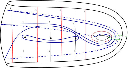
Figure 2. Intersection numbers with coordinate curves

If $L$ contains $p(c)$ many copies of $c$, then let

(1) $$c=-p(c),$$

where $p(c)>0$. Throughout the paper we define $c^{+}$ as $\max(c,0)$.

2.1. Path Components on $S_{n}$

In this section, we are going to introduce path components of an integral lamination $L$ on $S_{n}$ and derive formulas for the number of these components.

Let $U_{i}~{}(1\leq i\leq n)$ be the region that is bounded by $\beta_{i}$ and $\beta_{i+1}$ (Figure 3) and $G$ be the region bounded by $\beta_{1}$, $\beta_{n+1}$ and the boundary of $S_{n}$  ($\partial S_{n}$) (Figures  4 and 5). Since $L$ is minimal, there are $4$ types of path components in $U_{i}$  $(1\leq i\leq n)$ as on the disk [10]: Above component; which has end points on $\beta_{i}$ and $\beta_{i+1}$ intersecting with $\alpha_{2i-1}$, below component; which has end points on $\beta_{i}$ and $\beta_{i+1}$ intersecting with $\alpha_{2i}$, left loop component; which has both end points on $\beta_{i+1}$ intersecting with $\alpha_{2i-1}$ and $\alpha_{2i}$ (Figure 3 (a)) and right loop component; which has both end points are on $\beta_{i}$ intersecting with $\alpha_{2i-1}$ and $\alpha_{2i}$ (Figure 3 (b)). There are $6$ types of path components in $G$. First three are $c$ curve; bounding the genus of surface (Figure 4 (a)), front genus component; which has both end points on $\beta_{n+1}$ not intersecting with curve $c$ (Figure 4 (b)), back genus component; having both endpoints on $\beta_{1}$ not intersecting with curve $c$ (Figure 4 (c)). The other three components, called twisting which have end points on $\beta_{1}$ and $\beta_{n+1}$ intersecting with curve $c$ (see Figure 5) are non-twist component; see Figure 5 (a), negative twist component which makes clockwise twist (See Figure 5 (b)), and positive twist component which makes counterclockwise twist (See Figure 5  (c)).

\psfrag{a}[tl]{\scalebox{0.6}{$\scriptstyle{a}$}}\psfrag{b}[tl]{\scalebox{0.6}{$\scriptstyle{b}$}}\psfrag{a2i}[tl]{\scalebox{0.6}{$\scriptstyle{\alpha_{2i}}$}}\psfrag{a2i-1}[tl]{\scalebox{0.6}{$\scriptstyle{\alpha_{2i-1}}$}}\psfrag{bi}[tl]{\scalebox{0.6}{$\scriptstyle{\beta_{i}}$}}\psfrag{bi+1}[tl]{\scalebox{0.6}{$\scriptstyle{\beta_{i+1}}$}}\psfrag{d(2i-1)}[tl]{\scalebox{0.6}{$\scriptstyle{{\color[rgb]{0,0,1}\Delta_{2i-1}}}$}}\psfrag{d(2i)}[tl]{\scalebox{0.6}{$\scriptstyle{{\color[rgb]{0,0,1}\Delta_{2i}}}$}}\psfrag{U(i)}[tl]{\scalebox{0.6}{$\scriptstyle{U_{i}}$}}\includegraphics[width=281.85034pt]{puncture_bilesen}

Figure 3. Above and below components, left and right loop components in region $U_{i}$

\psfrag{a}[tl]{\scalebox{0.55}{$\scriptstyle{a}$}}\psfrag{b}[tl]{\scalebox{0.55}{$\scriptstyle{b}$}}\psfrag{g}[tl]{\scalebox{0.6}{$\scriptstyle{\gamma}$}}\psfrag{t}[tl]{\scalebox{0.6}{$\scriptstyle{c}$}}\psfrag{bn+1}[tl]{\scalebox{0.6}{$\scriptstyle{\beta_{n+1}}$}}\psfrag{b1}[tl]{\scalebox{0.6}{$\scriptstyle{\beta_{1}}$}}\includegraphics[width=390.25534pt]{genus_loop}

Figure 4. (a) $c$ curves, (b) front genus component, (c) back genus component in region $G$

\psfrag{a}[tl]{\scalebox{0.55}{$\scriptstyle{a}$}}\psfrag{b}[tl]{\scalebox{0.55}{$\scriptstyle{b}$}}\psfrag{g}[tl]{\scalebox{0.6}{$\scriptstyle{\gamma}$}}\psfrag{t}[tl]{\scalebox{0.6}{$\scriptstyle{c}$}}\psfrag{bn+1}[tl]{\scalebox{0.6}{$\scriptstyle{\beta_{n+1}}$}}\psfrag{b1}[tl]{\scalebox{0.6}{$\scriptstyle{\beta_{1}}$}}\includegraphics[width=390.25534pt]{cikis_yon}

Figure 5. (a) Non-twist component, (b) Negative twist component, (c) Positive twist component.

A twisting component’s twist number is the signed number of intersections with $\gamma$ curve.

Remark 2.1.

Since an integral lamination $L\in{\mathcal{L}}_{n}$ consists of simple closed curves that do not intersect each other, there can not be both curve $c$ and twisting components at the same time in the region $G$ (see Figure 6). Also note that there are a uniform front genus and a uniform back genus component in the region $G$.

\psfrag{a}[tl]{\scalebox{0.55}{$\scriptstyle{a}$}}\psfrag{b}[tl]{\scalebox{0.55}{$\scriptstyle{b}$}}\psfrag{g}[tl]{\scalebox{0.6}{$\scriptstyle{\gamma}$}}\psfrag{t}[tl]{\scalebox{0.6}{$\scriptstyle{c}$}}\psfrag{bn+1}[tl]{\scalebox{0.6}{$\scriptstyle{\beta_{n+1}}$}}\psfrag{b1}[tl]{\scalebox{0.6}{$\scriptstyle{\beta_{1}}$}}\includegraphics[width=216.81pt]{paralel_cikis}

Figure 6. $L$ does not contain both curve $c$ and twisting components at the same time.

Remark 2.2.

Note that the number $c^{+}$ gives the number of twisting components.

Remark 2.3.

Since an integral lamination does not contain any self-intersections, directions of the twists has to be the same. Also, in region $G$, the difference between the twist numbers of two different such components can not be greater than $1$ (see Figure 7).

\psfrag{a}[tl]{\scalebox{0.55}{$\scriptstyle{a}$}}\psfrag{b}[tl]{\scalebox{0.55}{$\scriptstyle{b}$}}\psfrag{g}[tl]{\scalebox{0.6}{$\scriptstyle{\gamma}$}}\psfrag{t}[tl]{\scalebox{0.6}{$\scriptstyle{c}$}}\psfrag{bn+1}[tl]{\scalebox{0.6}{$\scriptstyle{\beta_{n+1}}$}}\psfrag{b1}[tl]{\scalebox{0.6}{$\scriptstyle{\beta_{1}}$}}\includegraphics[width=216.81pt]{fark_big_zero}

Figure 7. If the difference between the twist numbers of two twisting components is greater than one, then they intersect.

If we denote the smaller twist number by $t$ and the bigger twist number by $t+1$, then the total twist number  $T$ in $G$ is the sum of the twist numbers of such components. Hence, if the difference between twist numbers of any two twisting components is $0$, then

$$T=tc^{+}.$$

On the other hand, if the difference between twist numbers of any two twisting components is $1$, then

$$T=m(t+1)+(c^{+}-m)t$$

where $m\in\mathbb{Z}_{\geq 0}$ is the number of twisting components with twist number $t+1$, and $c^{+}-m$ is the number of twisting components with twist number $t$.

Now, we calculate the path components of $L$ in $G$:

Lemma 2.4.

Let $L$ be given with the intersection numbers $(\alpha;\beta;\gamma;c)$, and the number of front genus components and the number of back genus components be $l$ and $l^{\prime}$, respectively. Then,

$$l=\frac{\beta_{n+1}-c^{+}}{2}\quad\text{ and }\quad l^{\prime}=\frac{\beta_{1}-c^{+}}{2}$$

Proof.

$\beta_{n+1}$ intersects only with twisting (Figure 5) and front genus (Figure 4 (b)) components. Since $\beta_{n+1}$ intersects once with each twisting component and twice with each front genus component, $\beta_{n+1}=c^{+}+2l$. From here, $l=\frac{\beta_{n+1}-c^{+}}{2}$ is derived. Similarly, $\beta_{1}$ intersects only with twisting (Figure 5) and back genus (Figure 4 (c)) components. Since $\beta_{1}$ intersects once with each twisting component and twice with each back genus component, $\beta_{1}=c^{+}+2l^{\prime}$. Therefore, $l^{\prime}=\frac{\beta_{1}-c^{+}}{2}$ is derived.       

In the following theorem, we calculate the total twist number of twisting components:

Lemma 2.5.

Let $L$ be given with the intersection numbers $(\alpha;\beta;\gamma;c)$, denoting the signed total twist number of twisting components by $T$. We have

(4) $$|T| =\left\{\begin{array}[]{ll}0&\mbox{if $c^{+}=0$},\\ \gamma-\frac{\beta_{n+1}-c^{+}}{2}-\frac{\beta_{1}-c^{+}}{2}&\mbox{if $c^{+}\neq 0$.}\end{array}\right.$$

The sign of the negative twist component is $-1$ and the sign of the positive twist component is $1$.

Proof.

Let us denote the total twist number of twisting components of $L$ by $|T|$. Note that the curve $\gamma$ intersects once with curve $c$ (Figure 4 (a)) and it intersects once with each front and back genus components (Figures 4 (b) and (c), respectively). Also, $\gamma$ intersects by the total number of twists of twisting components (Figure 5) with $L$. However, from Remark 2.1, there can not be twists and curve $c$ at the same time. Therefore, when $c^{+}\neq 0$, we have

(5) $$\gamma=l+l^{\prime}+|T|$$

where $l$,  $l^{\prime}$ and $|T|$ denote the number of front genus, back genus components and total twist number of twisting components, respectively.

From Lemma 2.4,

$$\gamma=\frac{\beta_{n+1}-c^{+}}{2}+\frac{\beta_{1}-c^{+}}{2}+|T|.$$

Hence,

$$|T|=\gamma-\frac{\beta_{n+1}-c^{+}}{2}-\frac{\beta_{1}-c^{+}}{2}.$$

    

By using the following theorem, we can calculate the number of curves $c$ (Figure 4 (a)):

Lemma 2.6.

Let $L$ be given with the intersection numbers $(\alpha;\beta;\gamma;c)$. The number of curves $c$ in $L$ is given by

(8) $$p(c) =\left\{\begin{array}[]{ll}\gamma-\frac{\beta_{n+1}}{2}-\frac{\beta_{1}}{2}&\mbox{if $c^{+}=0$},\\ 0&\mbox{if $c^{+}\neq 0$.}\end{array}\right.$$

Proof.

Since $c^{+}=0$, we can write $\gamma=l+l^{\prime}+p(c)$. From Lemma 2.4,

$$l=\frac{\beta_{n+1}}{2}\quad\text{ and }\quad l^{\prime}=\frac{\beta_{1}}{2}.$$

Hence, $p(c)=\gamma-\frac{\beta_{n+1}}{2}-\frac{\beta_{1}}{2}$ is derived.       

The twist numbers of each twisting component of an integral lamination whose intersection numbers are given are found by using Remark 2.3 and Lemma 2.5, which we find these twist numbers with the following lemma.

Lemma 2.7.

Let $L$ be given with the intersection numbers $(\alpha;\beta;\gamma;c)$. Let $|T|$ and $m$ be the total twist number and the number of twisting components which has $t+1$ twists, respectively. In this case,

(9) $$m\equiv|T|~{}(mod~{}c^{+})\quad\text{ and }\quad t=\frac{|T|-m}{c^{+}}$$

where $c^{+}\neq 0$.

Proof.

From Remark 2.3,

$$|T|=m(t+1)+(c^{+}-m)t.$$

From here, we have

$$|T|=m+tc^{+}.$$

Hence,

$$m\equiv|T|~{}(mod~{}c^{+})\quad\mbox{ and }\quad t=\frac{|T|-m}{c^{+}}$$

are derived.

    

Remark 2.8.

The intersection numbers $(\alpha;\beta;\gamma;c)$ might not always give an integral lamination. Because intersection numbers may not provide the conditions given in Lemma 2.10 or Lemma 2.11, and the triangle inequality in each region where is bounded by $\alpha_{2i-1}$,  $\alpha_{2i}$,  $\beta_{i}$ or by $\alpha_{2i-1}$,  $\alpha_{2i}$,  $\beta_{i+1}$.

To illustrate, we can not construct an integral lamination having the intersection numbers $(1,1,1,1,1,1;0,2,0,2;2;1)$. Because, according to Lemma 2.4, the numbers of front genus and back genus components are respectively

$$l=\frac{\beta_{4}-c^{+}}{2}=\frac{2-1}{2}=\frac{1}{2}\notin\mathbb{Z}_{\geq 0}\quad\mbox{ and }\quad l^{\prime}=\frac{\beta_{1}-c^{+}}{2}=\frac{0-1}{2}=-\frac{1}{2}\notin\mathbb{Z}_{\geq 0}.$$

In such a case, any integral lamination can not be constructed as shown in Figure 8.

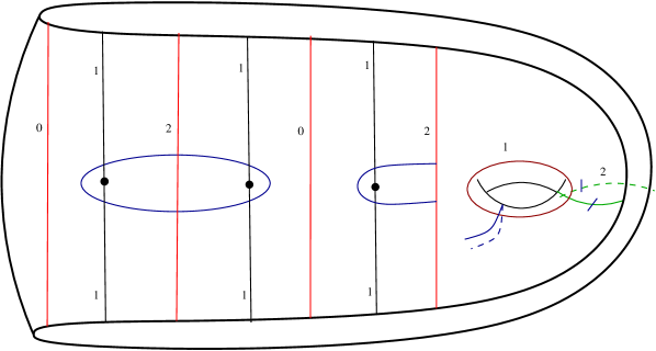
Figure 8. $\alpha_{2i}\cup\alpha_{2i-1}$ and $\beta_{i}$ are each even, however $c$ is odd.

Remark 2.9.

Let the number of loop components in each region $U_{i}$ for $1\leq i\leq n$ be denoted by $|b_{i}|$, where

(10) $$b_{i}=\frac{\beta_{i}-\beta_{i+1}}{2}.$$

If $b_{i}<0$, loop component is called left; if $b_{i}>0$, loop component is called right [4].

Lemma 2.10 ([9]).

The following equalities hold for each $U_{i}$:

When there is a left loop component,

$$\alpha_{2i}+\alpha_{2i-1}=\beta_{i+1}$$

$$\alpha_{2i}+\alpha_{2i-1}-\beta_{i}=2|b_{i}|,$$

when there is a right loop component,

$$\alpha_{2i}+\alpha_{2i-1}=\beta_{i}$$

$$\alpha_{2i}+\alpha_{2i-1}-\beta_{i+1}=2|b_{i}|,$$

when there is no loop components,

$$\alpha_{2i}+\alpha_{2i-1}=\beta_{i}=\beta_{i+1}.$$

Lemma 2.11.

Let $L$ be given with the intersection numbers $(\alpha;\beta;\gamma;c)$. Then for each $1\leq i\leq n$,  $\beta_{i}-\beta_{i+1}$ and $\alpha_{2i}-\alpha_{2i-1}-c^{+}$ are even.

Proof.

From Lemma 2.4, since

$$\beta_{n+1}=c^{+}+2l,$$

if $c^{+}$ is even (odd), $\beta_{n+1}$ is even (odd). Similarly, since

$$\beta_{1}=c^{+}+2l^{\prime},$$

if $c^{+}$ is even (odd), $\beta_{1}$ is even (odd). Also, from [4], the number of loop components is given by

$$b_{i}=\frac{\beta_{i}-\beta_{i+1}}{2}~{}(1\leq i\leq n).$$

From here, we can write

$$\beta_{i+1}=\beta_{i}-2\sum_{j=1}^{i}b_{j}.$$

Therefore, if $c^{+}$ is even (odd), each $\beta_{i}~{}(1\leq i\leq n+1)$ is even (odd).

From Lemma 2.10, when there is right loop component, $\alpha_{2i}+\alpha_{2i-1}=\beta_{i}$; when there is left loop component, $\alpha_{2i}+\alpha_{2i-1}=\beta_{i+1}$. Hence, when $c^{+}$ is even (odd), $\alpha_{2i}+\alpha_{2i-1}$ is even (odd).

Since when $c^{+}$ is even, $\alpha_{2i}+\alpha_{2i-1}$ is even and when $c^{+}$ is odd, $\alpha_{2i}+\alpha_{2i-1}$ is odd, $\alpha_{2i}+\alpha_{2i-1}-c^{+}$ is always even.

    

Lemma 2.12 ([4]).

Let $L\in{\mathcal{L}}_{n}$ be given with the intersection numbers $(\alpha;\beta;\gamma;c)$. For each $1\leq i\leq n$, the number of above, $u_{i}^{a}$, and below, $u_{i}^{b}$, components in $U_{i}$ can be found by

$$u_{i}^{a}=\alpha_{2i-1}-|b_{i}|\quad\mbox{ and }\quad u_{i}^{b}=\alpha_{2i}-|b_{i}|.$$

Remark 2.13.

The intersection numbers of two different integral laminations might be the same.

For example, while the intersection numbers of two integral laminations given in Figure 9 are $(2,2,2,2,2,2;2,4,2,4;4;2)$, since the twisting components of integral lamination in Figure 9 (a) twist in the negative direction and the twisting components of integral lamination in Figure 9 (b) twist in the positive direction, these integral laminations are different. Therefore, intersection numbers can not give an injective function.

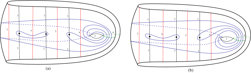
Figure 9. Two different integral laminations with the same intersection numbers

Remark 2.14.

Note that two different integral laminations might have the same intersection numbers (the directions of twisting components can be different). Therefore, we can derive an injective function from intersection numbers $(\alpha;\beta;\gamma;c)$ by giving a direction to the twists of twisting components.

Let $m_{i}=\min(\alpha_{2i}-|b_{i}|,\alpha_{2i-1}-|b_{i}|)$ and set $2a_{i}=\alpha_{2i}-\alpha_{2i-1}-c^{+}$ for $1\leq i\leq n$. By Lemma 2.11, $a_{i}$ is an integer. By similar calculations as in the way: disk case, we can derive the intersection number with $\alpha_{i}$ on $S_{n}$ in the following:

For each $1\leq i\leq 2n$,

(13) $$\alpha_{i} =\left\{\begin{array}[]{ll}\frac{2(-1)^{i}a_{\lceil i/2\rceil}+(-1)^{i}c^{+}+\beta_{\lceil i/2\rceil}}{2}&\mbox{if $b_{\lceil i/2\rceil}\geq 0$},\\ \frac{2(-1)^{i}a_{\lceil i/2\rceil}+(-1)^{i}c^{+}+\beta_{(1+\lceil i/2\rceil)}}{2}&\mbox{if $b_{\lceil i/2\rceil}\leq 0$}.\end{array}\right.$$

where $\lceil x\rceil$ is the smallest integer greater than or equal to $x$.

Now, we derive the intersection number with $\beta_{i}$ on $S_{n}$. Let $l$,  $l^{\prime}$ and $m_{i}$  $(1\leq i\leq n)$ show the front genus number, back genus number and the minimum of above and below component numbers, respectively. Since $L$ can not contain a curve that bounds the boundary, at least one of $m_{i}$,  $l$ or $l^{\prime}$ has to be $0$. There are two cases:

Case 1: Assume at least one of $m_{i}=0$ for $1\leq i\leq n$. In this case

(14) $$\beta_{n+1}=\max_{1\leq k\leq n}\left[2\max(b_{k},0)+|2a_{k}+c^{+}|-2\sum_{j=k}^{n}b_{j}\right]$$

and

(15) $$\beta_{n+1}\geq\max(c^{+},c^{+}-2\sum_{i=1}^{n}b_{i}).$$

An example for this case is depicted in Figure 10.

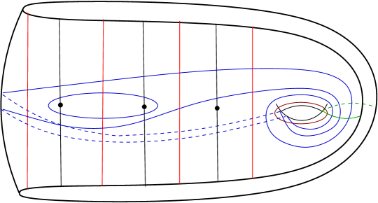
Figure 10. An integral lamination with $m_{i}\neq 0$ for $i=1,2$

Case 2: If $m_{i}\neq 0$ for any $1\leq i\leq n$: In this case, an integral lamination contains curves whose each above and below component number are different from $0$ (see Figure 11).

\psfrag{a}[tl]{\scalebox{0.55}{$\scriptstyle{\mbox{{(a)}}}$}}\psfrag{b}[tl]{\scalebox{0.55}{$\scriptstyle{\mbox{{(b)}}}$}}\includegraphics[width=433.62pt]{bad_start}

Figure 11. Integral laminations with each $m_{i}$ is different from $0$

Also, at least one of the front genus or back genus component numbers must be $0$. Otherwise, this curve system contains curves parallel to the boundary as shown in the Figure 12.

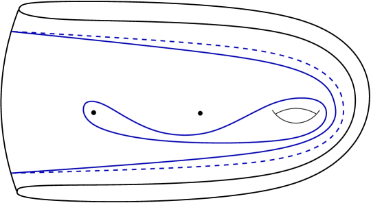
Figure 12. A curve system with a curve parallel to the boundary

Therefore, there are three possibilities:

1. If $l=l^{\prime}=0$ and $\sum_{i=1}^{n}b_{i}=0,$

2. If $l>0$, $l^{\prime}=0$ and $\sum_{i=1}^{n}b_{i}<0,$

3. If $l=0$, $l^{\prime}>0$ and $\sum_{i=1}^{n}b_{i}>0.$

Combining cases (i), (ii) and (iii), we get

(19) $$\beta_{n+1} =\left\{\begin{array}[]{ll}c^{+}-2\sum_{i=1}^{n}b_{i}&\mbox{if $\sum_{i=1}^{n}b_{i}<0$},\\ c^{+}&\mbox{if $\sum_{i=1}^{n}b_{i}>0$},\\ c^{+}&\mbox{if $\sum_{i=1}^{n}b_{i}=0$}.\end{array}\right.$$

Since each $m_{i}>0$ for $(1\leq i\leq n)$, we have

(20) $$\beta_{n+1}\geq\max_{1\leq k\leq n}\left[2\max(b_{k},0)+|2a_{k}+c^{+}|-2\sum_{j=k}^{n}b_{j}\right].$$

In terms of brevity, let

$$\kappa:=\max_{1\leq k\leq n}\left[2\max(b_{k},0)+|2a_{k}+c^{+}|-2\sum_{j=k}^{n}b_{j}\right].$$

From inequalities (15) and (20), we have

(21) $$\beta_{n+1}=\max(c^{+},c^{+}-2\sum_{i=1}^{n}b_{i},\kappa).$$

From Equation (10), for each $1\leq i\leq n$,

(22) $$\beta_{i}=2\sum_{j=i}^{n}b_{j}+\beta_{n+1}.$$

Now, we derive the intersection number with $\gamma$ on $S_{n}$. Since each path component in the region $G$, except non-twist twisting components, intersects with the arc $\gamma$ once, we have

$$\gamma=l+l^{\prime}+p(c),$$

if $p(c)\neq 0$, and when $p(c)=0$, we have

$$\gamma=l+l^{\prime}+|T|.$$

Recall that from Equation (1), $p(c)=-c$. Therefore,

(25) $$\gamma =\left\{\begin{array}[]{ll}|T|+l+l^{\prime}&\mbox{if $c>0$},\\ |c|+l+l^{\prime}&\mbox{if $c\leq 0$}.\end{array}\right.$$

By Lemma 2.4, and Equations (21) and (22), we have

(28) $$\gamma =\left\{\begin{array}[]{ll}|T|+\sum_{j=1}^{n}b_{j}+\max(c^{+},c^{+}-2\sum_{i=1}^{n}b_{i},\kappa)-c^{+}&\mbox{if $c>0$},\\ |c|+\sum_{j=1}^{n}b_{j}+\max(c^{+},c^{+}-2\sum_{i=1}^{n}b_{i},\kappa)-c^{+}&\mbox{if $c\leq 0$}.\end{array}\right.$$

Above we have expressed the intersection numbers with arcs $\alpha_{i}$, $\beta_{i}$ and $\gamma$ in terms of $a_{i}$, $b_{i}$ and $T$. Note that, for an integral lamination, $T=0$ when $c\leq 0$. Now, we can define Dynnikov coordinate system on $S_{n}$ which bijectively coordinatizes the set ${\mathcal{L}}_{n}$ .

Definition 2.15.

Let ${\mathcal{V}}_{n}=\{(a;b;T;c):c\leq 0\mbox{ and }T\neq 0\}\cup\{0\}.$ Dynnikov coordinate function $\Phi:{\mathcal{L}}_{n}\rightarrow\mathbb{Z}^{2n+2}\setminus{\mathcal{V}}_{n}$ on $S_{n}$ is defined by

$$\Phi(L)=(a;b;T;c)=(a_{1},\cdots,a_{n};b_{1},\cdots,b_{n};T;c)$$

where for each $1\leq i\leq n$,

(29) $$a_{i}=\frac{\alpha_{2i}-\alpha_{2i-1}-c^{+}}{2},\quad~{}b_{i}=\frac{\beta_{i}-\beta_{i+1}}{2}$$

and

(32) $$|T| =\left\{\begin{array}[]{ll}0&\mbox{if $c^{+}=0$},\\ \gamma-\frac{\beta_{n+1}-c^{+}}{2}-\frac{\beta_{1}-c^{+}}{2}&\mbox{if $c^{+}\neq 0.$}\end{array}\right.$$

Example 2.16.

We calculate the Dynnikov coordinates of the integral lamination shown in Figure 2.

Since $(\alpha_{1},\alpha_{2},\alpha_{3},\alpha_{4},\alpha_{5},\alpha_{6};\beta_{1},\beta_{2},\beta_{3},\beta_{4};\gamma;c)=(4,1,3,2,4,1;3,5,5,3;3;1),$ from Equations (29)

$$a_{1}=\frac{\alpha_{2}-\alpha_{1}-c^{+}}{2}=\frac{1-4-1}{2}=-2,$$

$$a_{2}=\frac{\alpha_{4}-\alpha_{3}-c^{+}}{2}=\frac{2-3-1}{2}=-1,$$

$$a_{3}=\frac{\alpha_{6}-\alpha_{5}-c^{+}}{2}=\frac{1-4-1}{2}=-2,$$

$$b_{1}=\frac{\beta_{1}-\beta_{2}}{2}=\frac{3-5}{2}=-1,$$

$$b_{2}=\frac{\beta_{2}-\beta_{3}}{2}=\frac{5-5}{2}=0,$$

$$b_{3}=\frac{\beta_{3}-\beta_{4}}{2}=\frac{5-3}{2}=1.$$

Also, since $c^{+}=\max(c,0)=\max(1,0)=1$, from Equation (32),

$$|T|=\gamma-\frac{\beta_{4}-c^{+}}{2}-\frac{\beta_{1}-c^{+}}{2}=3-\frac{3-1}{2}-\frac{3-1}{2}=1.$$

Since the twisting component twists in the negative direction, we derive $T=-1$. Hence, we find

$$\Phi(L)=(-2,-1,-2;-1,0,1;-1;1).$$

The following theorem Theorem 2.17 gives the inversion of Dynnikov coordinate function on $S_{n}$:

Theorem 2.17.

Let $(a;b;T;c)\in\mathbb{Z}^{2n+2}\setminus{\mathcal{V}}_{n}$. Then, the vector $(a;b;T;c)$ corresponds to one and only one integral lamination $L\in{\mathcal{L}}_{n}$ whose intersection numbers are given by

(33) $$\beta_{i}=2\sum_{j=i}^{n}b_{j}+\max(c^{+},c^{+}-2\sum_{i=1}^{n}b_{i},\kappa),\quad~{}\beta_{n+1}=\max(c^{+},c^{+}-2\sum_{i=1}^{n}b_{i},\kappa)$$

(36) $$\alpha_{i} =\left\{\begin{array}[]{ll}\frac{2(-1)^{i}a_{\lceil i/2\rceil}+(-1)^{i}c^{+}+\beta_{\lceil i/2\rceil}}{2}&\mbox{if $b_{\lceil i/2\rceil}\geq 0$},\\ \frac{2(-1)^{i}a_{\lceil i/2\rceil}+(-1)^{i}c^{+}+\beta_{(1+\lceil i/2\rceil)}}{2}&\mbox{if $b_{\lceil i/2\rceil}\leq 0$}.\end{array}\right.$$

and

(39) $$\gamma =\left\{\begin{array}[]{ll}|T|+\sum_{j=1}^{n}b_{j}+\max(c^{+},c^{+}-2\sum_{i=1}^{n}b_{i},\kappa)-c^{+}&\mbox{if $c>0$},\\ |c|+\sum_{j=1}^{n}b_{j}+\max(c^{+},c^{+}-2\sum_{i=1}^{n}b_{i},\kappa)-c^{+}&\mbox{if $c\leq 0$}.\end{array}\right.$$

where

$$\kappa=\max_{1\leq k\leq n}\left[2\max(b_{k},0)+|2a_{k}+c^{+}|-2\sum_{j=k}^{n}b_{j}\right].$$

Proof.

Let $L\in{\mathcal{L}}_{n}$ be an integral lamination whose Dynnikov coordinates are $\Phi(L)=(a;b;T;c)$.  Firstly, we shall show that Dynnikov function $\Phi:{\mathcal{L}}_{n}\rightarrow\mathbb{Z}^{2n+2}\setminus{\mathcal{V}}_{n}$ is injective. It has been shown in this paper that the intersection numbers corresponding to the minimal representative $L\in{\mathcal{L}}$ are as given in equations (33), (36) and (39). Then, the numbers of above, below, right loop or left loop components in each region $U_{i}$, the numbers of curves $c$, front genus, back genus, twisting components, the total twist of twisting components and the number of twists of each twisting component, the direction of these twists in the region $G$ are calculated as given in above, and therefore as indicated in Remark 2.14, the path components in regions $U_{i}$ and $G$ can be combined uniquely up to isotopy by giving a direction to the twists of twisting components. Hence, $\Phi$ is injective.

Now, we see that the function $\Phi\colon{\mathcal{L}}_{n}\rightarrow\mathbb{Z}^{2n+2}\setminus{\mathcal{V}}_{n}$ is surjective. Let $(a;b;T;c)\in\mathbb{Z}^{2n+2}\setminus{\mathcal{V}}_{n}$. We shall show that the intersection numbers $(\alpha;\beta;\gamma;c)$ defined by Equations (33), (36) and (39) correspond to an integral lamination $L\in{\mathcal{L}}_{n}$ such that $\Phi(L)=(a;b;T;c)$. First of all, it is easy to see that an integral lamination $L$ with intersection numbers $(\alpha;\beta;\gamma;c)$ should satisfy $\Phi(L)=(a;b;T;c)$. To get an integral lamination, we draw non-intersecting path components in each region and join them together.       

Example 2.18.

Let the Dynnikov coordinates of the integral lamination $L\in{\mathcal{L}}_{3}$ on $S_{3}$ be $\Phi(L)=(a;b;T;c)=(-2,-2,-1;0,-1,-1;-5;3)$. We find the intersection numbers corresponding to the minimal representative $L$.

Since $c=3>0$, $p(c)=0$ and $c^{+}=3$. From Theorem 2.17, the intersection numbers $\alpha$, $\beta$ and $\gamma$ are found as the following:

When we place the given Dynnikov coordinates to the equation

$$\kappa=\max_{1\leq k\leq 3}\left[2\max(b_{k},0)+|2a_{k}+c^{+}|-2\sum_{j=k}^{3}b_{j}\right],$$

we find $\kappa=5$. From here,

$$\beta_{4} =\max(c^{+},c^{+}-2\sum_{i=1}^{3}b_{i},\kappa)$$

$$=\max(3,3-2(0-1-1),5)=7,$$

that is, $\beta_{4}=7$. From Equation (22), we derive

$$\beta_{1}=2(b_{1}+b_{2}+b_{3})+\beta_{4}=2(0-1-1)+7=3.$$

By the similar calculations, we have $\beta_{2}=3$ and $\beta_{3}=5$. From Equation (36), since $b_{1}=0$, $\alpha_{1}=2$ and $\alpha_{2}=1$. Since $b_{2}<0$, $\alpha_{3}=3$ and $\alpha_{4}=2$. Since $b_{3}<0$, $\alpha_{5}=3$ and $\alpha_{6}=4$. Since $c>0$, from Equation (39),

$$\gamma =|T|+\sum_{j=1}^{3}b_{j}+\max(c^{+},c^{+}-2\sum_{i=1}^{3}b_{i},\kappa)-c^{+}$$

$$=|T|+b_{1}+b_{2}+b_{3}+\max(c^{+},c^{+}-2(b_{1}+b_{2}+b_{3}),\kappa)-c^{+}$$

$$=5+0-1-1+\max(3,3-2(0-1-1),5)-3=7.$$

Now, we calculate the numbers of path components in the regions $G$ and $U_{i}$. Since $c^{+}=3$ and $T=-5$, there are $3$ twisting components and the total number of twists is $5$ (see Remark 2.2 and Lemma 2.5), and twisting components twist in the negative direction. By Lemma 2.7, there are $2$ twisting components, which each twisting component does $2$ twists, and there is $1$ twisting component doing $1$ twist. According to Lemma 2.4,

$$l=\frac{\beta_{4}-c^{+}}{2}=\frac{7-3}{2}=2\quad\mbox{ and }l^{\prime}=\frac{\beta_{1}-c^{+}}{2}=\frac{3-3}{2}=0.$$

That is, there are $2$ front genus components, however there is not any back genus component.

From Equation (10),

$$b_{1}=\frac{\beta_{1}-\beta_{2}}{2}=\frac{3-3}{2}=0.$$

Similarly, we have $b_{2}=-1$ and $b_{3}=-1$. Namely, there are no loop components in region $U_{1}$,  $1$ left loop component in region $U_{2}$ and $1$ left loop component in region $U_{3}$.

The numbers of above and below components in each $U_{i}$ are:

$$u_{1}^{a}=\alpha_{1}-|b_{1}|=2-0=2\quad~{}\mbox{ and }~{}\quad u_{1}^{b}=\alpha_{2}-|b_{1}|=1-0=1.$$

That is, there are $2$ above components and $1$ below component in $U_{1}$. By similar calculations, we find $2$ above and $1$ below components in $U_{2}$ and $2$ above and $3$ below components in $U_{3}$.

The integral lamination $L$ in Figure 13 is derived uniquely by combining the calculated components up to isotopy.

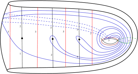
Figure 13. $\Phi(L)=(a;b;T;c)=(-2,-2,-1;0,-1,-1;-5;3)$

Remark 2.19.

The Dynnikov coordinates for integral laminations on $S_{n}$ obtained in this paper can be extended in a natural way to Dynnikov coordinates of measured foliations on $S_{n}$.

Acknowledgements: The author would like to thank her advisor Saadet Öykü Yurttaş and co-advisor Semra Pamuk and point out that the results in this paper are part of author’s PhD thesis.

References

- [1] M. Bestvina, M. Handel, Train-tracks for surface homeomorphisms, Topology, 34(1), 109–140, 1995.
- [2] P. Dehornoy, I. Dynnikov, D. Rolfsen, B. Wiest, Why are braids orderable?, Panoramas et Syntheses [Panoramas and Syntheses]. Societe Mathematique de France, Paris, 14, 2002.
- [3] P. Dehornoy, Efficient solutions to the braid isotopy problem, Discrete Appl. Math., 156(16), 3091–3112, 2008.
- [4] I. Dynnikov, On a Yang-Baxter mapping and the Dehornoy ordering, Uspekhi Mat. Nauk, 57(3(345)), 151–152, 2002.
- [5] A. Haas, P. Susskind, The connectivity of multicurves determined by integral weight train tracks, Trans. Amer. Math. Soc. 329, 2, 637–652, 1992.
- [6] H. Hamidi-Tehrani, Z. Chen, Surface diffeomorphisms via train-tracks, Topology Appl., 73(2), 141–167, 1996.
- [7] J. Moussafir, On computing the entropy of braids, Funct.Anal. Other Math., 1, 37–46, 2006.
- [8] R.C. Penner, J. L. Harer, Combinatorics of train tracks, Annals of Mathematics Studies. Princeton University Press, Princeton, NJ, 125, 1992.
- [9] S.Ö. Yurttaş,T. Hall, On the topological entropy of families of braids, Topology and its Applications 158(8), 1554–1564, 2009.
- [10] S.Ö. Yurttaş, Geometric intersection of curves on punctured disks, Journal of the Mathematical Society of Japan, 65(4), 1554–1564, 2013.
- [11] S.Ö. Yurttaş, T. Hall, Intersections of multicurves from Dynnikov coordinates, Bull. Aust. Math. Soc. 98(1), 149–158, 2018.