Optomechanical cavity without a Stokes side-band

Abstract

We investigate a theoretical demonstration of perfect frequency conversion in an optomechanical system in the weak coupling regime without a Stokes side-band. An optomechanical cavity illuminated by a weak probe field generates two side-modes, differentiating from the original signal by a phonon frequency. We report the presence of a special combination of parameters in the weak-coupling regime, where Stokes side-mode vanishes exactly. Only the anti-Stokes mode is observed with a few hundreds Hz spectral bandwidth of the probe field. Emergence of this special point is totally unrelated with the electromagnetically induced transparency (EIT) condition, where absorption (dip) cancellation is limited with the damping rate of the mechanical oscillator. Emergence is independent of the cavity type, i.e. single or double-sided, and takes place only for a single value of the effective coupling strength constant which is specific to the system parameters. At a specific effective coupling strength between the mirror and the cavity field, which can be tunable via the coupling field, only the anti-Stokes band is generated. At that specific coupling there appears no Stokes field. Hence, a filter, to eliminate the Stokes field, does not necessitate.

The field of cavity optomechanics investigates the coupling between light inside an optical cavity and a mechanical oscillator via radiation pressure force Aspelmeyer et al. (2014). This coupling leads to alter light from one cavity resonance to another resonance of a different frequency in the strong coupling regime without loss. Optomechanically induced transparency in a membrane for optomechanical cavity setup system was observed experimentally Karuza et al. (2013).The optical properties of the optomechanical system Weis et al. (2010); Agarwal and Huang (2010) controlled by the motion of the mechanical oscillator in a cavity revealed challenging applications Verhagen et al. (2012a); Palomaki et al. (2013); McGee et al. (2013); Zhang et al. (2003), especially optomechanical frequency conversion Hill et al. (2012); Kale et al. (2015); Andrews et al. (2014); Lecocq et al. (2016). The conversion between optical fields by using photon-phonon translation in a cavity optomechanical system has been observed recently Hill et al. (2012). And also a wavelength conversion of light in silicon nitride microdisk resonators has been proposed experimentally Kale et al. (2015). In addition to optical conversion, efficient conversion between microwave and optical light has been demonstrated reversibly and coherently in the classical regime Andrews et al. (2014). Finally, microwave frequency conversion via the motion of a mechanical resonator has been observed experimentally in the quantum regime Lecocq et al. (2016). A optical frequency conversion can be used in critical functions such as a quantum network Kimble (2008). Cavity optomechanics systems allow for fundamentally new forms of quantum information Stannigel et al. (2012) and optomechanical light storage Fiore et al. (2011). Since not only photons are non-interacting particles but also insensitive to environmental distortion, photons are preferred for optical communication and quantum information processing which requires interaction. The interaction between light inside an optical cavity and a mechanical oscillator can be used for this procedure. Optomechanical systems have become attractive for quantum optomechanical memory Safavi-Naeini et al. (2011) and quantum state transfer Verhagen et al. (2012b, c) very recently.

The coupling between light inside an optical cavity and a mechanical oscillator can be used in telecommunications for signal modulation since this type of interaction leads to change the frequency of the incident beam and its wavelength Hill et al. (2012). In this work, we investigate the frequency conversion via an optomechanical system operating in the weak coupling regime without a Stokes side-band. In an optomechanical cavity system, mechanical frequency (nanomechanical oscillator of frequency $\omega_{m}$) will modulate the probe laser with frequency $\omega_{p}$ and will form a new sidebands frequency $2\omega_{L}-\omega_{p}$, which is called anti-Stokes sidebands. We find that the conversion can be controlled by the optomechanical coupling strength and detuning. We report the presence of a special combination of parameters in the weak-coupling regime($g\ll\kappa,\gamma$), where Stokes side-mode vanishes exactly. Only the anti-Stokes mode is observed with a few hundreds Hz spectral bandwidth. Emergence of this special point is totally unrelated with the EIT condition, where absorption cancellation is limited with the damping rate of the mechanical oscillator. Emergence is independent of the cavity type, i.e. single or double-sided, and takes place only for a single value of the effective coupling constant which is specific to the system parameters. We report a theoretical demonstration of the frequency conversion in an optomechanical system in the weak coupling regime. Beside the microwave frequency conversion by the motion of a mechanical resonator  Lecocq et al. (2016) our system show that by tuning the probe field at a special interaction strength $g$ the classical optical field can be inverted without loss.

Firstly, we briefly describe the Hamiltonian of the systems. We obtain the Heisenberg equations and then we get the first order solutions analytically. An optomechanical system consists of an optical cavity and a nanomechanical mirror which can be treated as nano mechanical oscillator(NMO). NMO is located at the center of the cavity. The cavity field (frequency $\omega_{c}$) is driven by an external strong source with frequency $\omega_{L}$ and a weak probe field of frequency $\omega_{p}$.

The probe field $\varepsilon_{p}$ is treated as classical and the response of the cavity optomechanical system to the probe field in the presence of the coupling field $\varepsilon_{L}$ is computed. Mechanical-cavity field coupling is provided by presence of an coupling laser. The mass and resonance frequency of an nanomechanical oscillator is $m$ and $\omega_{m}$ respectively. NMO is coupled to a Fabry-Perot cavity via radiation pressure effects  Aspelmeyer et al. (2014). In a Fabry-Perot cavity, both mirrors have equal reflectivity. We use a configuration in which a partially transparent NMO is in the middle of a cavity that is bounded by two high-quality mirrors as shown in Fig.  1.

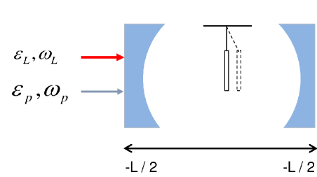
Figure 1: (Color online) Schematic of a double-ended cavity with a moving nanomechanical mirror. The length of the cavity is $L$. The classical probe field $\varepsilon_{p}$ and the coupling field $\varepsilon_{L}$ are applied to the cavity.

The Hamiltonian of this system is given by  Tarhan et al. (2013)

$$H = \hbar\Delta_{c}c^{\dagger}c-\hbar g_{0}c^{\dagger}cq+\frac{p^{2}}{2m}+\frac{1}{2}m\omega_{m}^{2}q^{2}$$ (1)

$$+ i\hbar\varepsilon_{L}(c^{\dagger}-c)+i\hbar(c^{\dagger}\varepsilon_{p}e^{-i\Delta_{p}t}-c\varepsilon_{p}^{\ast}e^{i\Delta_{p}t}).$$

$\Delta_{c}=\omega_{c}-\omega_{L}$, $\Delta_{p}=\omega_{p}-\omega_{L}$ are the frequencies of cavity and probe field. $g_{0}=\omega_{c}/L$ is the coupling constant between the cavity field and the movable mirror  Bhattacharya et al. (2008), $q_{0}$ is the steady state position of the movable mirror and $c,c^{\dagger}$ are the annihilation creation and operators of the photons of the cavity field respectively. The momentum and position operators of the nanomechanical oscillator are $p$ and $q$, respectively. $\varepsilon_{L}$ is taken to be real while $\varepsilon_{p}$ is taken to be complex. The amplitude of the pump field is $\varepsilon_{L}=\sqrt{2\kappa P_{L}/\hbar\omega_{L}}$ with $P_{L}$ being the pump power.

Heisenberg equation of motion for the coupled cavity-mirror system is written and the damping rate $2\kappa$ is added phenomenologically to represent the loss at the cavity mirrors where $\kappa$ is the decay rates of the cavity mirrors. The damping rate of the mechanical oscillator is $\gamma$. Here we neglect the quantum and thermal noise and examine the system in the mean field limit  Agarwal and Huang (2010); Tarhan et al. (2013). The linear response solution was developed analytically:  Tarhan et al. (2013)

$$c(t)=c_{0}+c_{+}\varepsilon_{p}e^{-i\Delta_{p}t}+c_{-}\varepsilon_{p}^{\star}e^{i\Delta_{p}t}.$$ (2)

If we solve Heisenberg equation of motion by using the linear response solution Boyd (2003); Tarhan et al. (2013), we will get the steady state solutions $c_{0}=\varepsilon_{L}/(2\kappa+i\Delta)$, $q_{0}=-\hbar g|c_{0}|^{2}/m\omega_{m}^{2}$ and the first order solutions $c_{+}$ and $c_{-}$  Tarhan et al. (2013):

$$c_{+} = \frac{A\times B-i\omega_{m}|g|^{2}}{[(\kappa-i\Delta_{p})^{2}+\Delta^{2}]\times B+2\omega_{m}\Delta|g|^{2}}$$

$$c_{-} = \frac{i|g|^{2}\omega_{m}}{[(\kappa-i\Delta_{p})^{2}+\Delta^{2}]\times B+2\omega_{m}\Delta|g|^{2}},$$ (3)

where $\Delta=\Delta_{c}-g_{0}q_{0}$ is the effective detuning, $A=[\kappa-i(\Delta+\Delta_{p})]$, $B=(\Delta_{p}^{2}-\omega_{m}^{2}+i\gamma_{m}\Delta_{p})$, $g=g_{0}c_{0}$ is the effective coupling, $|c_{0}|^{2}$ is the resonator intensity which is obtained from steady state equations, and $q_{0}$ is the steady state position of the movable mirror.

The output field can be obtained by using the input-output relation $\varepsilon_{out}=2\kappa\langle c\rangle$ Huang (2014). According to linear solution written in Eq. (2) , we expand the output field to the first order in the probe field $\varepsilon_{p}$ and find the output field as

$$\varepsilon_{out}(t)=\varepsilon_{out0}+\varepsilon_{out+}\varepsilon_{p}e^{-i\Delta_{p}t}+\varepsilon_{out0-}\varepsilon_{p}^{*}e^{i\Delta_{p}t},$$ (4)

where $\varepsilon_{out0}$, $\varepsilon_{out+}$, and $\varepsilon_{out-}$ are the components of the output field oscillating at frequencies $\omega_{L}$, $\omega_{p}$, and $2\omega_{L}-\omega_{p}$. The terms $e^{\pm i2\Delta_{p}t}$ are not taken into account because we are interested in the linear response Refs. Agarwal and Huang (2010); Tarhan et al. (2013); Boyd (2003).

In our calculations, we use experimental parameters Thompson et al. (2008) for the length of the cavity $L=6.7$ cm, the wavelength of the coupling laser $\lambda=2\pi c/\omega_{c}=1064$ nm, $m=40$ ng, $\omega_{m}=2\pi\times 134$ kHz, $\gamma=0.76$ Hz, $\kappa=\omega_{m}/10$, and $\Delta=\omega_{m}$. Analytical demonstration of the first order solutions are given in Fig.  2. We show the real and the imaginary parts of the $c_{+}$ and $c_{-}$ In Fig.  2. In order to cancel the Stokes field, we equalize the absolute value of numerator $c_{+}$ to the zero. After solving the cubic equation, we get only one real value $\Delta_{p}=0.999995486667198\omega_{m}$ at critical coupling strength $g=0.0043\omega_{m}$. This special point is totally unrelated with the EIT condition, where absorption cancellation is limited with the damping rate of the mechanical oscillator.

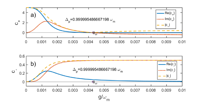
Figure 2: The analytical solution $c_{+}$ and $c_{+}$ as a function of the optomechanical coupling strength. The parameters used are the length of the cavity $L=6.7$ cm, the wavelength of the laser $\lambda=2\pi c/\omega_{c}=1064$ nm, $m=40$ ng, $\omega_{m}=2\pi\times 134$ kHz, $\gamma=0.76$ Hz, $\kappa=\omega_{m}/10$ and $\Delta_{p}=0.999995486667198\omega_{m}$, $\Delta=\omega_{m}$ and $g_{cr}=0.0043\omega_{m}$.

The value of imaginary and real parts $c_{+}$ are both 0 when the probe detuning at a special point $\Delta_{p}=0.999995486667198\omega_{m}$. It has been easily seen in Fig.  2 that imaginary and real parts of $c_{+}$ are zero in the weak-coupling regime $g=0.0043\omega_{m}$. One can infer from Fig.  2 that the component of the output field oscillating at frequency $\omega_{p}$ disappears whereas the component of the output field oscillating at frequency $2\omega_{L}-\omega_{p}$ will occur.

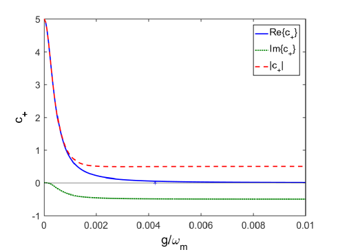
Figure 3: The analytical solution $c_{+}$. The parameters are the same as in Fig. 2, except that $\Delta_{p}=\omega_{m}$ (EIT condition).

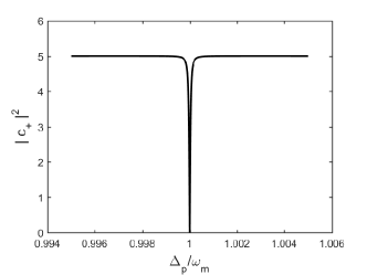
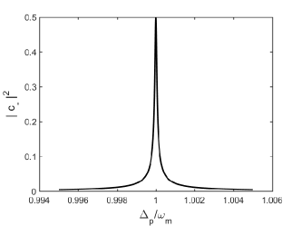
Figure 4: (a) The intensity $|c_{+}|^{2}$ as a function of the probe detuning $\Delta_{p}$. (b) The intensity $|c_{-}|^{2}$ as a function of the probe detuning $\Delta_{p}$. The parameters used for both curves are the same as in Fig. 2.

At the same time we plot the $c_{+}$ as a function of $g$ in Fig. 3 when the probe detuning $\Delta_{p}=\omega_{m}$ in order to show the importance of the special point. As seen in in Fig.  3 the value of imaginary part of $c_{+}$ is different from 0 at the probe detuning $\Delta_{p}=\omega_{m}$.

Moreover, we plot the intensity spectrums $|c_{+}|^{2}$ and $|c_{-}|^{2}$ as a function of the probe detuning $\Delta_{p}$ in Fig. 4. As seen in Fig. 4 a few hundreds Hz spectral bandwidth of the probe field(only the anti-Stokes mode) is observed. The value of $|c_{+}|^{2}$ is completely is 0 whereas the value of $|c_{-}|^{2}$ is about 0.25 when the probe detuning $\Delta_{p}=0.999995486667198\omega_{m}$ at a critical coupling strength $g=0.0043\omega_{m}$. The intensity of the $|c_{+}|^{2}$ which is called linear response vanishes at these special points. At these points the linear response disappears and anti-Stokes field occurs which is shown in Figs.  2 and  4. In the presence of a special combination of parameters in the weak-coupling regime, where Stokes side-mode vanishes exactly. Only the anti-Stokes mode is observed with a few hundreds Hz spectral bandwidth.

We have reported a theoretical demonstration of perfect frequency conversion in an optomechanical system in the weak coupling regime without a Stokes side-band. We have converted the classical optical fields with frequency $\omega_{p}$ to another optical fields with frequency $2\omega_{L}-\omega_{p}$. We report the presence of a special combination of parameters —in the weak-coupling regime, e.g. $g=0.0043\omega_{m}$— where Stokes side-mode vanishes exactly. This property is clearly beneficial for demonstration of frequency conversion in an optomechanical setup which is formed by vibrating mirror under the action of a strong coupling field. It has been shown that, in the a few hundreds Hz spectral width of the probe field, only the anti-Stokes mode is observed.

Furthermore we have computed the intensity spectrum of the probe field. Our results reveal that by tuning the probe field at a special interaction strength $g$ the classical optical field can be inverted without loss. This result can be useful for quantum information processing because there is no signal loss in our system.