Ab initio models of atomic nuclei:
challenges and new ideas

Abstract

This review presents some of the challenges in constructing models of atomic nuclei starting from theoretical descriptions of the strong interaction between nucleons. The focus is on statistical computing and methods for analyzing the link between bulk properties of atomic nuclei, such as radii and binding energies, and the underlying microscopic description of the nuclear interaction. The importance of careful model calibration and uncertainty quantification of theoretical predictions is highlighted.

1 Keywords:

Nuclear interactions, chiral effective field theory, model calibration, uncertainty quantification, optimization, Bayesian parameter estimation.

2 Introduction

The ab initio approach to describe atomic nuclei and nuclear matter is grounded in a theoretical description of the interaction between the constituent protons and neutrons. The long-term goal with this course of action is to construct models to describe and analyze the properties of nuclear systems with maximum predictive power. It is of course well known that the elementary particles of the strongly interacting sector of the Standard Model are quarks and gluons, not protons and neutrons. However, since the relevant momentum scales of typical nuclear structure phenomena are low enough to not resolve the internal degrees of freedoms of nucleons, it is reasonable to model the nucleus as a collection of strongly interacting and point-like nucleons. This idea has inspired significant efforts aimed at developing algorithms and mathematical approaches for solving the many-nucleon Schrd̈oinger equation in a bottom-up fashion and with as few uncontrolled approximations as possible, see e.g. Refs. [1, 2, 3, 4, 5, 6, 7], as well as a multitude of theoretical descriptions of the interaction between nucleons, at various levels of phenomenology, see e.g. Refs. [8, 9, 10], and Refs. [11, 12, 13] for comprehensive reviews on (chiral) effective field theory (EFT) methods. Reference [14] also offers a historical account of various approaches to understand the nuclear interaction.

Currently, ab initio modelling of atomic nuclei face two main challenges:

• We have limited knowledge about the details of the interaction between nucleons, which in turn limits our ability to predict nuclear properties.

• Given a microscopic description of the interaction between nucleons inside a nucleus, a quantum-mechanical solution of the nuclear many-body problem is exacerbated by the curse of dimensionality.

There is however continuous progress on both frontiers, and attempts at quantifying the uncertainty of model predictions are beginning to emerge in the community. Rapid algorithmic advances in combination with a dramatic increase in available computational resources make it possible to employ several complementary mathematical methods for solving the nuclear Schrödinger equation. We can nowadays generate numerical representations of microscopic many-nucleon wavefunctions, for selected medium-mass and heavy-mass nuclei, with a rather impressive precision. Although several observables remain beyond the reach of state-of-the-art models, e.g. most properties associated with highly collective states, we can still describe certain classes of observables rather well, such as total ground-state binding energies and radii, and sometimes low-energy excitation spectra. We are thus capable of analyzing experimentally relevant nuclei directly in terms of a quantum mechanical description of the interaction between its constituent nucleons. Indeed, the list of, sometimes glaring, discrepancies between theory and experiment furnish some of the most interesting nuclear physics questions at the moment, see e.g. Refs. [15, 16, 17, 18, 19, 20, 21]. Many of these efforts are aimed understanding the nuclear binding mechanism, the location of the neutron dripline, the existence of shell-closures and magic numbers in exotic systems, and the emergence of nuclear saturation.

State-of-the-art theoretical analyses of experimental data indicate a large and non-negligible systematic uncertainty in the description of bulk nuclear observables, see e.g. Ref. [22]. Given the high-precision of modern many-body methods, much of this uncertainty can be traced to the description of the interaction potential. Although there exists ab initio models that describe nuclei rather well, albeit in a limited domain, it is less clear why other models sometimes fail. Indeed, the NNLO_sat interaction potential [23] reproduces several key experimental binding energies and charge radii for nuclei up to mass $A\sim 50$ [24, 25, 26, 21], while the so-called 1.8/2.0 (EM) interaction potential [27, 28] reproduces binding energies and low-energy spectra up to mass $A\sim 100$ [24, 29, 30, 31, 32, 33] while radii are underestimated. The origin of the differences between these potentials is unknown. It is of course the role of nuclear theory to close the gap between theory and experiment by developing and refining the theoretical underpinnings of the model. But given the complex nature of atomic nuclei, there is significant value in trying to quantify, or estimate, the detailed structure of the observed theoretical uncertainty. This might provide important clues about where we should focus our efforts. There exists well-defined statistical inference methods that can provide additional guidance, and several ongoing projects are currently focused on applying statistical computing methods in the field of ab initio modelling. The topic of uncertainty quantification in nuclear physics has been discussed at a series of workshops on Information and Statistics in Nuclear Experiment and Theory (ISNET). Recent developments in this field are documented in the associated focus issue published in Journal of Physics G [34]. A second focus issue has just been announced, and the first few papers are already published.

In Sec. 3 and Sec. 4 of this paper I will review a selection of recent results and often applied methods for calibrating ab initio models. In Sec. 5 and Sec. 6 I will discuss some of the recently emerging strategies for making progress using statistical computing and Bayesian inference methods. The aim is to provide an overview of selected accomplishments in the field of statistical inference and statistical computing with ab initio models of atomic nuclei. Hopefully, this paper can serve as a brief introduction to practitioners who wish to learn about ongoing developments and possible future directions.

As a final remark, in this paper I will try to consistently use the word model when referring to any current method for theoretically describing the properties of atomic nuclei, including descriptions that claim to be building on more fundamental underpinnings, such as EFT. One can certainly make a finer distinction between models, EFTs, and theories. As outlined in Ref. [35]; theories provide a unified framework, categorization, and the joint language used for discussions; EFTs capture physics at a given momentum scale; and models can be used to study aspects of a theory, increase understanding, and provide intuition.

3 Ab initio models of nuclear many-body systems

An ab initio model is here defined as a description that is based on wavefunctions $|\Psi\rangle$ that solve the many-nucleon Schrödinger equation

$$[\hat{T}+\hat{V}(\vec{\alpha})]|\Psi\rangle=E|\Psi\rangle.$$ (1)

In this schematic representation, $\hat{T}$ is the total kinetic energy operator for the $A$-nucleon system, $\hat{V}(\vec{\alpha})$ is the potential energy operator for the interaction between the nucleons, and $E$ is the total energy of the system in the state represented by $|\Psi\rangle$. The potential operator term depends on a set of parameters $\vec{\alpha}$ that governs the strengths of the various interaction pieces in the potential. Below I will also refer to these parameters as low-energy constants (LECs). Given a particular expression for the potential $\hat{V}$, with numerical values for the parameter vector $\vec{\alpha}$, and a mathematical method to solve Eq. 1 for e.g. the state $|\Psi\rangle$ with lowest energy, it is in principle possible to quantitatively compute the expectation value for any observable $\hat{\mathcal{O}}$ with respect to this state, e.g. its charge radius. Of course the trustworthiness of the result and its level of agreement with experimental data can vary dramatically between different models, i.e. combinations of potentials and many-body methods.

I will denote an ab initio model with $M(\vec{\alpha},\vec{x})$. It is defined as the combination of a definite expression for the potential $\hat{V}(\vec{\alpha})$, and a method for solving the Schrödinger equation. The vector $\vec{x}$ is a set of control inputs that specify all necessary settings such as nucleon numbers, which observable to compute, values of the fundamental physical constants, and algorithmic settings for the mathematical method used for solving Eq. 1. Once a set of numerical values for $\vec{\alpha}$ has been determined, a subset of the control inputs $\vec{x}$ of the model can be varied to make model predictions, preferably at some physical setting, for e.g. exotic nuclei where we cannot easily make measurements. Provided that the form of the potential operator $\hat{V}$ and relevant physical constants remain the same, and the model parameters $\vec{\alpha}$ were calibrated carefully, it is of course possible to transfer the vector $\vec{\alpha}$ between ab initio models based on different methods for solving the many-nucleon Schrödinger equation. This is also in line with a physical interpretation of the parameters $\vec{\alpha}$ that elevate them to a status beyond being simple tunable parameters inherent to a specific model with the sole purpose of achieving a good fit to calibration data. This will be discussed further in Sec. 4.

One of the most exciting developments in nuclear theory is that we nowadays have access to a range of methods for solving Eq. 1 with very high numerical precision for selected isotopes and observables. This gives us the opportunity to compare model predictions with experimental data to learn more about the elusive structure of the interaction between nucleons. However, such an analyses require careful statistical interpretation of the theoretical results. In particular a sensible estimate of the uncertainty associated with a theoretical prediction. Indeed, only with reliable theoretical errors is it possible to infer the significance of a disagreement between experiment and theory, which in turn may hint at new physics.

3.1 Chiral potentials and the strong interaction between nucleons

On a fundamental level, the atomic nucleus is a quantum mechanical and self-bound system of interacting nucleons. In turn these particles are composed of three quarks whose mutual interactions are described well by the Standard Model of particle physics. As such, starting from the Standard Model it should be possible to account for all observed phenomena also in atomic nuclei, besides possible signals of beyond Standard Model physics. However, to theoretically understand the emergence of nuclei from the Standard Model is an open problem, and linking the quantitative predictions of atomic nuclei to the dynamics of quarks and gluons is a central challenge in low-energy nuclear theory. Although, viewing the atomic nucleus as a (color-singlet) composite multi-quark system is not the most economical choice. Indeed, the strong interaction, which is the most important component for nuclear binding and well-described by quantum chromodynamics (QCD), is non-perturbative in the low-energy region inhabited by atomic nuclei. Non-perturbative Monte Carlo sampling of the quantum fields of QCD amounts to a computational problem of tremendous proportions. This strategy, referred to as lattice QCD, is expected to require at least exascale resources for a realistic analysis of even the lightest multi-nucleon systems. Without any unforeseen disruptive technology, this approach will not provide an operational method for routine analyses of nuclei. For the cases where numerically converged results can be obtained, lattice QCD offers a unique computational laboratory for theoretical studies of QCD in a low-energy setting, see e.g. Ref. [36, 37].

The description of nuclei should nevertheless build on QCD, or the Standard Model in general. A turning point in the development of QCD-based descriptions of the nuclear interaction came when EFTs of QCD [38] arrived also to many-nucleon physics [39]. An EFT formulates the dynamics between low-energy degrees of freedom, e.g. nucleons and pions, in harmony with some assumed symmetries of an underlying theory, e.g. QCD, and any high-energy dynamics, e.g. quark-gluon interactions, are integrated out of the theory. The resulting chiral effective Lagrangian models the low-energy interactions between two or more nucleons in terms of pion exchanges between nucleons and the high-energy dynamics is incorporated as zero-ranged contact interactions. This approach introduces several model parameters referred to as low energy constants (LECs). They were denoted with $\vec{\alpha}$ above, and play a central role during the model calibration discussed below. The notion of high- and low-energy scales in EFT requires the presence of at least two scales in the physical system under study. An EFT formally exploits this scale separation to expand observables in powers of the low-energy (soft) scale over the high-energy (hard) scale, and in chiral EFT the resulting ratio is often denoted

$$Q=\frac{{\rm max}[m_{\pi},k]}{\Lambda_{b}}$$ (2)

where, in the case of chiral EFT, the soft scales are $m_{\pi}$ and $k$, the pion mass and a typical external momentum scale, respectively. The hard scale is denoted $\Lambda_{b}$ and is set by the e.g. the nucleon mass $M_{N}$. Depending on the system under study, one can always try to exploit existing scale separations to construct other kinds of EFTs in nuclear physics, e.g. pion-less EFT [40], vibrational EFT [41], or chiral perturbation theory (the prototypical EFT of QCD) [42]. In the following, I will only discuss results from ab initio models based on chiral EFT, i.e. a pion-full EFT, but many of the methods can be generally applied.

In chiral EFT, the nuclear interaction potential $V$ is analyzed as an order-by-order expansion in terms of $Q^{\nu}$ and organized following the principles of an underlying power counting (PC). Terms at a higher chiral expansion-orders $\nu$ should be less important than terms at a lower orders. Potentials expanded to higher orders are expected to describe data better. Higher chiral orders contain more involved pion exchanges and polynomial nucleon-contacts of increasing exponential dimension, and therefore more undetermined model parameters $\vec{\alpha}$ to handle during the calibration stage. To provide some detail about the chiral potentials: the leading-order (LO) typically consists of the familiar one-pion exchange interaction plus a nucleonic contact-potential. The structure of the contact potential, and the exact treatment of sub-leading orders vary depending on the PC. Still, typical chiral potentials include at most contributions up to a handful of chiral orders, e.g. next-to-next-leading order (NNLO) and next-to-next-to-next-to-leading order (N3LO), and the total number of LECs, i.e. undetermined model parameters, range between $\sim 10-20$, sometimes a few more. Some of the unique advantages of chiral EFT descriptions of the nuclear interaction are the natural emergence of two-, three-, and many-nucleon interactions [43, 44, 45, 46], the consistent formulation of quantum currents, e.g. with respect to electroweak operators [47, 48, 49, 50], and a clear connection with the pion-nucleon Lagrangian which makes it possible to link nuclei with low-energy pion-nucleon scattering processes [51]. For a detailed account of chiral EFT potentials, see Refs. [11, 12, 13].

To ensure steady progress towards a realistic ab initio model for atomic nuclei, we need to critically examine and evaluate the quality and predictive power of different theoretical approaches and model predictions. To this end it is crucial to equip all quantitative theoretical results with uncertainties, and this is where another advantageous aspect of EFT comes into play. It promises to deliver a handle on the systematic uncertainty of a theoretical prediction. Indeed, on a high level the EFT expansion for an observable $\mathcal{O}$ can be written

$$\mathcal{O}=\mathcal{O}_{0}\sum_{\nu=0}^{\infty}c_{\nu}Q^{\nu},$$ (3)

where $\mathcal{O}_{0}$ is the first term in the above expansion, and $c_{\nu}$ are dimensionless expansion coefficients. Here, and in the following, the LO result ($\mathcal{O}_{0}$) was pulled out in front of the sum to set the overall scale. One could equally well use the experimental value for $\mathcal{O}$ or the highest-order calculation to set the scale of the observable expansion. If we are dealing with an EFT, one should expect the expansion coefficients to be of natural size such that predictions at successive chiral orders are smaller by a factor of $Q$. See also Refs. [52, 53] for discussions on how to assess the convergence of data. In an actual calculation, the order-by-order description of $\mathcal{O}$ is truncated at some finite order $k$, which induces a truncation error $\delta_{k}$ in the prediction. The underlying EFT description then, in principle, allows us to determine the formal structure of the truncation error

$$\delta_{k}=\mathcal{O}_{0}\sum_{\nu=k+1}^{\infty}c_{\nu}Q^{\nu}.$$ (4)

This type of handle on the theoretical uncertainty in a prediction is not present in purely phenomenological descriptions of the nuclear interaction such as the Argonne V18 potential [8] or the CD-Bonn potential [9]. Despite all of the promised advantages of chiral EFT, it should be pointed out that much work remains to be done regarding the analysis and theoretical underpinnings of chiral EFT, in particular the formulation of a PC that, arguably, fulfills the field theoretic requirements for an EFT of QCD, see e.g. Refs. [54, 55, 56, 57, 58, 59, 60, 61] for various views on this topic. Indeed, one cannot yet confidently claim that the uncertainty estimates in ab initio predictions of nuclear observables based on proposed chiral EFT interactions are linked to missing physics at the level of the effective Lagrangian. The details of the PC, regularization approach, and chosen maximum chiral order $k$ in Eq. 3, are some of many possible choices that give rise to the rich landscape of different chiral interactions in nuclear theory. Although there is a flurry of activity, and far from clear which is the best way to proceed, there is tremendous overarching value to organize the model analysis according to the fundamental ideas and expectations of EFT, most importantly the promise of order-by-order improvement.

4 Model Calibration

The goal of model calibration is to learn about the parameter of the model using a pool of calibration data. This can mean many different things depending on the situation, and in this section I will discuss a few representative model calibration examples from ab initio nuclear theory.

Assume that we have a model $M(\vec{\alpha};\vec{x})$ that consists of a method for solving the Schrödinger equation and some theoretical description of the nuclear interaction, e.g. a particular interaction potential from chiral EFT, and we do not know the permissible values for $\vec{\alpha}$. The vector $\vec{\alpha}=[\alpha_{1},\alpha_{2},\ldots,\alpha_{N}]$ denotes the $N$ physically relevant and adjustable calibration parameters of model $M$, and the vector $\vec{x}$ denotes the set of control inputs. The adjustable parameters of interest will typically correspond to the LECs of the nuclear interaction potential, and the vector $\vec{x}$ will contain e.g. proton- and neutron-numbers, observable type, or some kinematical setting. In principle the model might contain additional adjustable parameters that for some reasons can be considered as constants. For instance, we typically do not consider the pion mass as a calibration parameter, although the variation of such fundamental properties can also play an important role, see e.g. Refs. [62, 63]. The choice of many-body method will depend on which class of observables is targeted, either during prediction or calibration. For instance, coupled-cluster theory will perform very well for nuclei in the vicinity of closed shells and Faddeev integration will be able to access the positive energy spectrum of the three-nucleon Hamiltonian. Throughout, I will implicitly assume that the model is realized only on a computer, i.e. $M$ is defined through some computer code, and there is no stochastic element present in the output. This means that each time the model is evaluated with the same input and settings, we will basically get the same result.

To calibrate the parameters, suppose that we have a set of $n$ experimental observations compiled in a data vector $D=[z_{1},z_{2},\ldots,z_{n}]$. They correspond to particular settings $\vec{x}_{1},\vec{x}_{2},\ldots,\vec{x}_{n}$ of the control variables, to produce model outputs for e.g. ground-state energies for light nuclei or scattering cross sections at selected scattering momenta. We can link the data points to the model outputs via the following relation

$$z_{i}=M(\vec{\alpha},\vec{x}_{i})+\delta(\vec{x}_{i})+\varepsilon_{i}.$$ (5)

This expression relates the reality of measurement with our model, and includes a so-called model discrepancy term $\delta$, that depends on the control variable $\vec{x}_{i}$. The measurement error is denoted with $\varepsilon_{i}$. In cases where the measurement is accompanied with zero uncertainty, something that is highly unlikely of course, the model discrepancy term represents the entire difference between the model and reality. The theoretical discrepancy $\delta$ is not physics per se, but should rather be interpreted as a random variable of statistical origin, informed via domain knowledge.

The model discrepancy term can be partitioned into at least three terms

$$\delta(\vec{x}_{i})=\delta_{\rm interaction}(\vec{x}_{i})+\delta_{\rm many-body}(\vec{x}_{i})+\delta_{\rm numerical}(\vec{x}_{i}),$$ (6)

and they represent the neglected or missing physics in the theoretical description of the nuclear interaction, neglected or missing many-body correlations in the mathematical solution of the many-body Schrödinger equation, and any numerical errors arising due to algorithmic approximations in the implementation of the computer model, respectively. We are currently most interested in understanding $\delta_{\rm interaction}$ in situations where we, to a good approximation, can neglect $\delta_{\rm many-body}$ and $\delta_{\rm numerical}$. Thus, in most of the literature, the dominant part of the model discrepancy originates from the chiral EFT description of the nuclear interaction. It should be pointed out that the discrepancy term of the many-body method can be quite large for many types of observables. However, ab initio methods are often applied wisely, and there exists plenty of domain knowledge regarding which many-body methods that are best suited for different kinds of observables. Yet, it is not easy to set bounds on this discrepancy a priori. Comparison between several complementary ab initio models provides important validation [64, 65, 66]. Finally, the last term in Eq. 6 is currently not the dominant part of the discrepancy, provided that the computer code has been benchmarked.

Two related questions immediately arise: i) what is the impact of the discrepancy term $\delta(\vec{x}_{i})$ on the inference about the model parameters $\vec{\alpha}$? and ii) what happens if we neglect all sources of model discrepancy during model calibration?

Let us consider the second question, since it is easier and also sheds light on the first one. Ignoring $\delta(\vec{x}_{i})$ in Eq. 5 leaves us with the following expression

$$z_{i}=M(\vec{\alpha},\vec{x}_{i})+\varepsilon_{i}.$$ (7)

This is the conventional starting point in nuclear model calibration. If one also assumes that the measurement errors $\varepsilon_{i}$ have finite variance, then the principle of maximum entropy dictates that the likelihood of the data is normally distributed. For independent errors, this leads to the canonical expression for the likelihood

$$\begin{split}P(D|\vec{\alpha},M,\sigma){}&=\prod_{i=1}^{n}\frac{1}{\sqrt{2\pi}\sigma_{i}}{\rm exp}\left\{-\frac{(z_{i}-M(\vec{\alpha},\vec{x}_{i}))^{2}}{2\sigma_{i}^{2}}\right\}\\ {}&=\left[\prod_{i=1}^{n}\frac{1}{\sqrt{2\pi}\sigma_{i}}\right]{\rm exp}\left\{-\frac{1}{2}\sum_{j=1}^{n}\frac{(z_{j}-M(\vec{\alpha},x_{j}))^{2}}{\sigma_{j}^{2}}\right\}\\ {}&=\left[\prod_{i=1}^{n}\frac{1}{\sqrt{2\pi}\sigma_{i}}\right]{\rm exp}\left\{-\frac{1}{2}\chi^{2}(\vec{\alpha})\right\}.\end{split}$$ (8)

Here, the notation $P(X|Y)$ denotes the pdf of $X$ conditioned on $Y$. The structure of the likelihood remains the same for correlated measurement errors, although one must employ the full covariance matrix instead of only the diagonal terms $\sigma_{j}^{2}$ to represent the variance of the data. Model calibration in ab initio nuclear theory is typically formulated as a maximum likelihood problem. This boils down to finding the optimal, or best-fitting, parameters $\vec{\alpha}_{\star}$ that minimize the exponent in Eq. 8. We are thus facing a mathematical optimization (minimization) problem

$$\vec{\alpha}_{\star}=\underset{\vec{\alpha}\in\Omega}{\textnormal{arg min}},\,\chi^{2}({\vec{\alpha}}),$$ (9)

of finding the point that fulfills $\chi^{2}(\vec{\alpha}_{\star})\leq\chi^{2}(\vec{\alpha})$ for all $\vec{\alpha}\in\Omega$, where $\Omega$ represents the parameter domain. In general, this is an intractable problem unless we have detailed information about $\vec{\alpha}$ or that the parameter domain is discrete and contains a finite number of points. In reality, we are trying to find local minimizers to $\chi^{2}(\vec{\alpha})$, i.e. points $\vec{\alpha}_{\star}$ for which $\chi^{2}(\vec{\alpha}_{\star})\leq\chi^{2}(\vec{\alpha})$ for all $\vec{\alpha}\in\Omega$ close to $\vec{\alpha}_{\star}$.

For ab initio models, optimization of the likelihood function typically proceeds in several steps [8, 9, 10, 67, 68, 69]. First, the parameters, i.e. the LECs in chiral EFT, are calibrated such that the model optimally reproduces nucleon-nucleon scattering phase-shifts from published partial-wave analyses [70, 71]. This typically yield model parameters confined to some narrow range of values. Although each scattering phase-shift only depends on a limited subset of the entire vector of model parameters $\vec{\alpha}$, this stage still benefits from using mathematical optimization algorithms, such as the derivate-free algorithm called pounders [72, 73]. In a next step, the results from the phase-shift optimization serves as the starting point for a second round of parameter optimization where all model parameters are varied to best reproduce thousands of nucleon-nucleon scattering cross sections up to scattering energies in the vicinity of the pion-production threshold.

Minimizing the $\chi^{2}$ in Eq. 8 for nucleon-nucleon interaction potentials with respect to nucleon-nucleon scattering data has been the workhorse of model calibration in nuclear theory for decades. Since long, the figure of merit for a nuclear interaction potential has been the $\chi^{2}$-per-datum value. If this value is close to unity for some particular parameterization $\vec{\alpha}_{\star}$, then the corresponding potential is dubbed to be ’high-precision’. This is beginning to change. Only for models $M$, where the model-discrepancy is in fact negligible this approach can be justified. Otherwise, chasing a low $\chi^{2}$ leads down the path of significant over-fitting, with unreliable predictions as a consequence. For the calculation of nucleon-nucleon scattering phase shifts and cross sections it is valid to ignore $\delta_{\rm many-body}$ and $\delta_{\rm numerical}$ since the corresponding equations are can be solved more or less numerically exactly. However, since we clearly cannot claim to have a zero-valued $\delta_{\rm interaction}$ term, the $\chi^{2}$-per-datum with respect to nucleon-nucleon scattering data is not the optimal measure to guide future efforts in nuclear theory. Before and during the development of ab initio many-body methods and EFT principles, when it was very unclear how to understand the concept of model discrepancy in nuclear theory, it was certainly more warranted to benchmark nuclear potentials based solely on a straightforward $\chi^{2}$ value.

State-of-the-art interaction potentials also contain three-nucleon force terms. Although some of the parameters in chiral EFT are shared between two- and three-nucleon terms, there exists a subset of parameters inherent only to the three-nucleon interaction. Such parameters must be determined using observables from $A>2$ systems. Arguably, all parameters of a chiral potential should be optimized simultaneously to a joint dataset $D$. The parameters must therefore be informed about e.g. binding energies and charge radii of ^3,4He and ³H. Unfortunately, there exists a universal correlation between the binding energies of ³H and ⁴He, the so-called Tjon line [75], which reduces the information content of this data set. Ground state-energies and radii are also highly correlated. Fortunately, it was demonstrated in Ref. [76] that the beta decay of ³H can add valuable information about the parameters in the three-nucleon interaction. Most methods for solving the $A=2,3,4$ Schrödinger equation for bound states do so with nearly zero many-body discrepancy. Recently, selected three-nucleon scattering observables have been added to the pool of calibration data [77], however not routinely since it is still computationally quite costly to evaluate the ab initio models for such observables. There are indications that it is necessary to include also data from nuclei heavier than ⁴He to learn about the parameters in ab initio models. This is discussed in Sec. 4.2.

Ignoring the $\delta_{\rm interaction}$ discrepancy terms during model calibration can have serious consequences. Most importantly, this reduces the LECs to tuning parameters without any physical meaning. Indeed, in the strive to replicate the data at any cost, the numerical values can be driven far away from the true values of the model. At some point, continued tuning of the parameters induces over-fitting and the model will pick up on the noise in the data. Naturally , this leads to poor predictive power. With increasing amounts of data, the optimization process will converge with increasing certainty to false values for $\vec{\alpha}$. A pedagogical introduction to the statistics of model discrepancies and a physics example is provided in Ref. [78].

A total model discrepancy, according to Eq. 6, was included in ab initio model calibration for the first time in Ref. [67]. The parameters in a set of chiral interactions at LO, NLO, and NNLO were optimized using nucleon-nucleon, and pion-nucleon scattering data. The terms in the three-nucleon interaction were simultaneously informed using bound-state observables from $A=2,3$ nuclei. The details of the analysis and results can be found in the original paper. The discrepancy terms were interpreted as uncorrelated errors and added in quadrature with the data uncertainties, leading to a slight modification of the corresponding $\chi^{2}$ function

$$\chi^{2}=\sum_{j=1}^{n}\frac{(z_{j}-M(\vec{\alpha},x_{j}))^{2}}{\sigma_{{\rm data},}j^{2}+\sigma^{2}_{{\rm interaction},j}+\sigma^{2}_{{\rm many-body},j}+\sigma^{2}_{{\rm numerical},j}}.$$ (10)

The interaction discrepancy was constructed from the EFT assumption that the external momenta flowing through the interaction diagrams scale as some power corresponding to the truncation of the chiral expansion, in accordance with Eq. 4. The intrinsic scale of this error was solved for self-consistently by requiring that the $\chi^{2}$-per-datum should approach unity providing that the model error is correctly estimated. This implicitly assumes a correct estimate of the number of statistical degrees of freedom. Something that cannot be easily estimated for non-linear $\chi^{2}$ functions [79].

To summarize, although the inclusion of model discrepancies is preferred, it is not without problems. To blindly include a term $\delta(\vec{x}_{i})$ to capture model discrepancies in the process of model calibration can lead to statistical confounding between $\vec{\alpha}$ and $\delta(\cdot)$ [78]. This means that the model parameters and the discrepancy term are not identifiable and we only recover a some joint pdf for the two components. Indeed, for any $\vec{\alpha}$ there is a $\delta(\cdot)$ given by the difference between model and reality. To make progress requires us to specify some a priori ranges for $\vec{\alpha}$ and/or $\delta(\cdot)$. Or in the language of Bayesian inference, we need to specify the prior pdf for the model parameters and the theory uncertainties. This is partly related to approaches where one augments the $\chi^{2}$ function with a penalty term to constrain the values of the model parameters, see e.g. Ref. [80]. For EFT descriptions of the nuclear interaction one can argue that the LECs should maintain values of order unity, if expressed in units of the breakdown scale, and the discrepancy could follow the pattern of Eq. 4. To adequately represent the discrepancy term in nuclear models is ongoing research , and it appears advantageous to reformulate model calibration as a Bayesian inference problem, see Sec. 5.

4.1 Hessian error analysis

At the optimum parameter point $\vec{\alpha}_{\star}$, a Taylor expansion of the $\chi^{2}$ function to second order gives

$$\begin{split}\chi^{2}(\vec{\alpha}_{\star}+\Delta\vec{\alpha}){}&\approx\chi^{2}(\vec{\alpha}_{\star})+\frac{1}{2}(\Delta\vec{\alpha})^{T}H(\Delta\vec{\alpha}),\\ {}&{\rm where}\,\,\,\left.H_{ij}=\frac{\partial^{2}\chi^{2}(\vec{\alpha})}{\partial\alpha_{i}\partial\alpha_{j}}\right|_{\vec{\alpha}=\vec{\alpha}_{\star}},\end{split}$$ (11)

where $H$ denotes a Hessian matrix, the inverse of which is proportional to the covariance matrix for the model parameters [81]. Contracting the parameter-Jacobian of any model prediction with this covariance matrix yields the standard error propagation result of the parameter uncertainties. For the conventional $\chi^{2}$ function, the parameter covariances reflect the impact of the experimental uncertainties on the precision of the optimum and predicted observables. Sometimes, this is referred to as statistical uncertainties, which is a bit confusing since all uncertainties are statistical in nature. See Fig. 1 for an example result of applying a parameter covariance matrix to obtain the joint pdf for the ⁴He ground-state energy and the ²H point-proton radius, two important few-nucleon observables. This particular result is taken from Ref. [67], where in fact a model discrepancy term $\delta(\cdot)$ was incorporated during the optimization, thus in this particular case the covariances reflect more than just the measurement noise. See e.g. Refs. [82, 83, 84, 85, 86, 87] for details about statistical error analysis and illuminating examples of forward error propagation in ab initio nuclear theory.

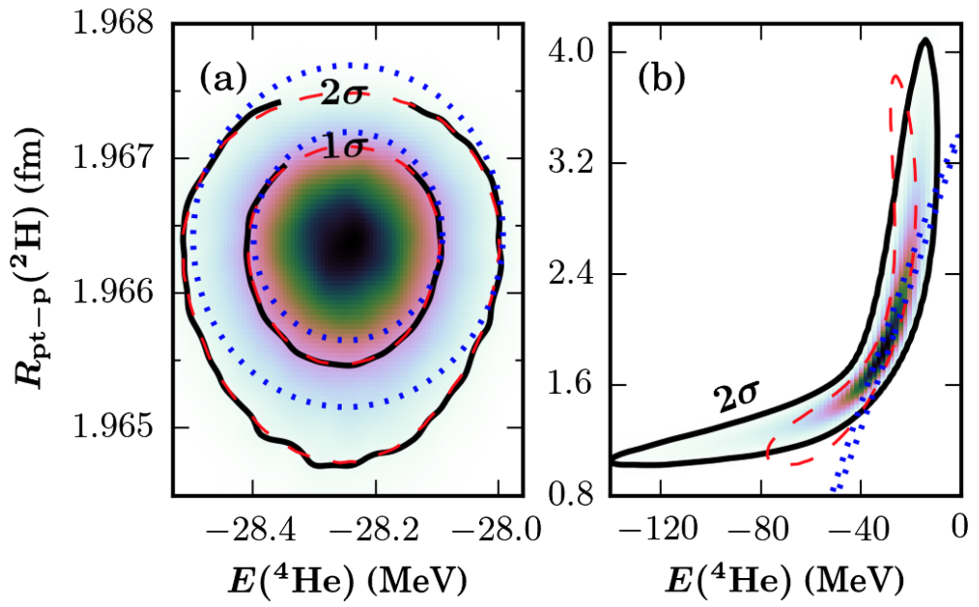
Figure 1: Joint distribution for the ground-state energy of ⁴He (x-axis) and the point-proton radius of ²H (y-axis) for (a) the chiral potential NNLO_sim and (b) the chiral potential NNLO_sep, see Ref.  [67]. Contour lines for the distributions are shown as black solid lines, while blue dotted (red dashed) contours are obtained assuming a linear (quadratic) dependence on the LECs for the observables.

To extract the covariance matrix requires computation of the second-order derivatives of the $\chi^{2}$ function with respect to the model parameters. The general process of numerically differentiating an ab initio model with respect to $\vec{\alpha}$ is significantly simplified, and numerically much more precise, with the use of automatic differentiation (AD) [67]. This corresponds to applying the chain rule of differentiation on a function represented as a computer code. It relies on the principle that any computer code, no matter how complicated always executes a set of elementary arithmetic operations on a finite set of elementary functions (exponentiation, logarithmization, etc). To implement AD requires modification of the original computer code, e.g. operator overloading via third-party libraries. Once implemented, AD also enables application of more advanced derivative-based optimization algorithms and Markov chain Monte Carlo methods with the computer model $M$. An alternative, and derivative-free approach, to computing the Hessian matrix for forward error propagation is to employ Lagrange multipliers [88]. This method is more robust, but also more computationally demanding to carry out. From a practical and computational perspective, if one considers to use Lagrange multipliers, one should also look into performing a Bayesian analysis, see Sec. 5.

4.2 Selecting calibration data

It is preferable to use data corresponding to observables that are computationally cheap to evaluate, and if possible with model settings corresponding to low $\delta(\vec{x})_{\rm many-body}$ discrepancies. One should also strive to include data with highly complementary information content that constrain a maximum amount of linearly independent combinations of model parameters.

The conventional approach to calibrate ab initio models is to use only data from $A\lesssim 4$ nuclei, as was discussed above. It was observed in Ref. [23] that the additional inclusion of ground-state energies and charge radii of selected carbon and oxygen isotopes dramatically increases the predictive power of models for bulk properties of nuclei up to the medium-mass nickel region, see Fig, 2. This calibration strategy led to the construction of the so-called NNLO_sat interaction. From a quantitative perspective, the advent of models capable of accurate predictions is of course an important step forward and has proven very useful [24, 25, 89, 90].

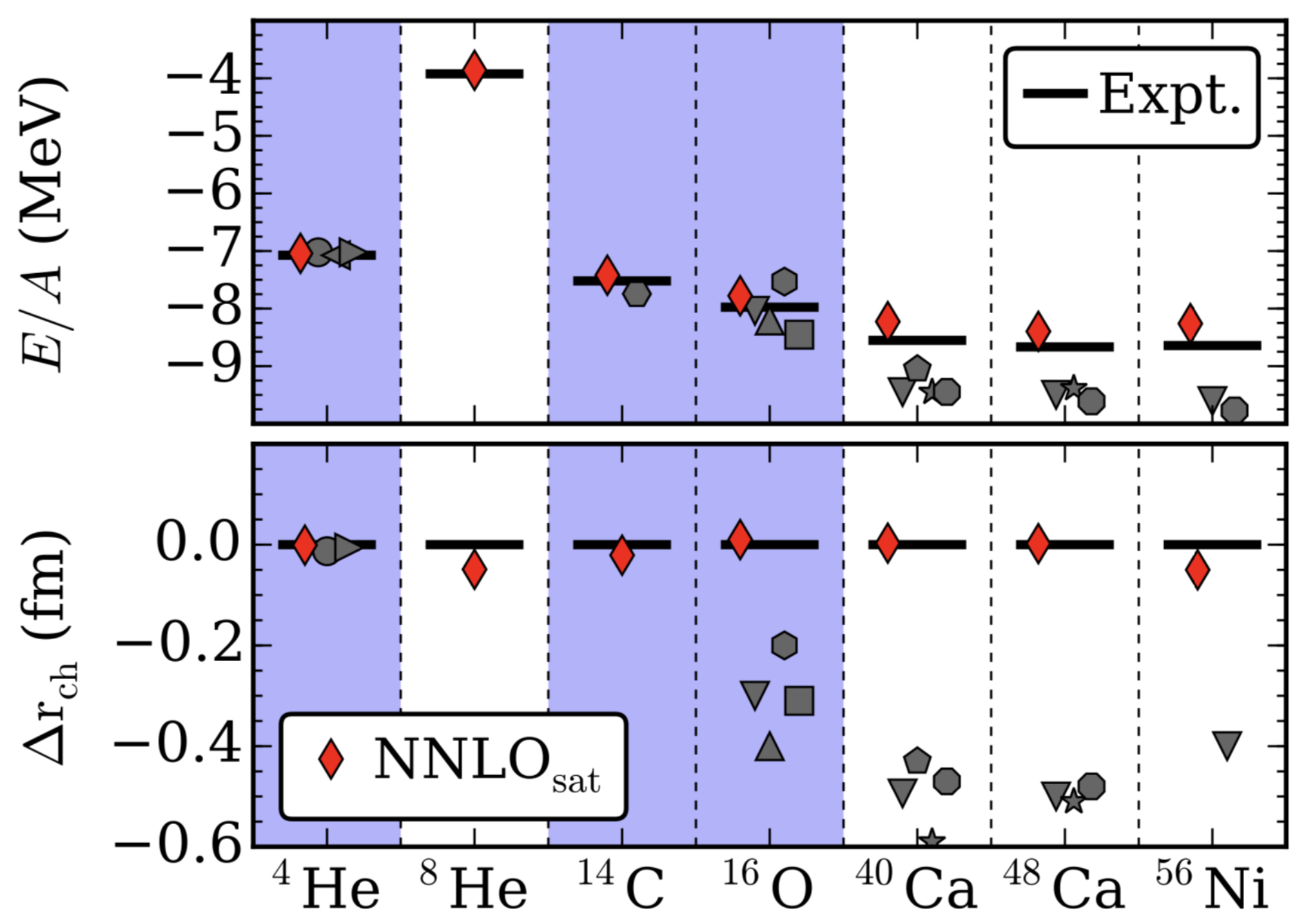
Figure 2: Ground-state energies per nucleon (top) and differences between theoretical and experimental charge radii (bottom) for selected light and medium-mass nuclei and results from ab initio computations. The red diamonds mark results based on the chiral interaction NNLO_sat. The blue columns indicate which nuclei where included in the optimization of the LECs in NNLO_sat, while the white columns are predictions. Grey symbols indicate other chiral interactions.

The major drawback of any model based on the NNLO_sat interaction is the lack of quantified theoretical uncertainties. This is quite common also for ab initio models based on other interaction potentials. At the moment, the best we can do is to estimate the truncation error using Eq. 4. This requires additional and sub-leading chiral-order potentials using the same optimization protocol, e.g. LO_sat and NLO_sat, which do not exist. The calibration of such models require an even more careful inclusion of model discrepancies. This is discussed more in Sec. 5. One can certainly argue that it becomes even more important to quantify the theory errors for models that we strongly believe will make accurate predictions, like the ones based on the NNLO_sat interaction. Otherwise we are limited in our ability to assess discrepancies with respect to experiment. This argument applies equally well to models based on e.g. the 1.8/2.0 interaction from Ref. [27, 28] which typically yield good predictions for binding energies and low-energy spectra. In Ref. [24], the prediction from ab initio models based on different interactions, NNLO_sat and the 1.8/2.0 interactions amongst other, were compared to estimate the overall theoretical uncertainty.

It is difficult to judge the degree of over-fitting to finite nuclei in NNLO_sat. It was noted during calibration that this interaction fails to reproduce experimental nucleon-nucleon scattering cross sections for scattering momenta larger than $\sim m_{\pi}$. Enforcing a good reproduction of all scattering data up to e.g. the pion-production threshold most likely corresponds to over-fitting in the $A=2$ sector. It is the role of the model discrepancy term, with appropriate priors, to balance this.

One clearly gains predictive power by including additional medium-mass data during the calibration stage. This was also observed in a lattice EFT analysis of the nuclear binding mechanism [91]. The related topic of possibly emergent nuclear phenomena like saturation, binding, and deformation of atomic nuclei is discussed further in Ref. [92]. Although the inclusion of a model discrepancy term while calibrating to heavier-mass data will be important, it does not solve the underlying problem of having a systematically uncertain model. It was noted in Refs. [93, 94, 95] that the explicit inclusion of the $\Delta$ isobar in the chiral description of the nuclear interaction dramatically improves the description of nuclei while also reproducing nucleon-nucleon scattering data. A possibly fruitful way forward is to employ improved models, i.e. with explicit inclusion of the $\Delta$ isobar, that are calibrated using also data from selected heavy-mass nuclei, while systematically accounting for model discrepancies. Furthermore, it will be interesting to se how much additional information is contained in three-nucleon scattering data [96].

5 Bayesian inference

The previous section introduced the concept of model calibration and the fundamental expression in Eq. 5 that relates a model with measured data. In this section I will outline the Bayesian strategy for learning about the model parameters and some existing estimates of the discrepancy term. The overarching goal is still to calibrate an ab initio model $M(\vec{\alpha},\vec{x})$, and reliably predict properties of atomic nuclei. However, instead of finding a single point $\vec{\alpha}_{\star}$ in parameter space that maximizes the likelihood for the data, we can use Bayes’ theorem to relate the data likelihood to a pdf for the model parameters themselves

$$P(\vec{\alpha}|D,M,I)=\frac{P(D|\vec{\alpha},M,I)P(\vec{\alpha}|M,I)}{P(D|M,I)},$$ (12)

where $P(\vec{\alpha}|M,I)$ denotes the prior pdf for the parameters, $P(D|\vec{\alpha},M,I)$ denotes the likelihood of the data, the denominator $P(D|M,I)$ denotes the marginal likelihood of the data, and $P(\vec{\alpha}|D,M,I)$ denotes the sought-after posterior pdf of the model parameters. The additional $I$ represents any other information at hand.

The Bayesian reformulation of the inference problem can at first sight appear as a subtle point, and it is easy to overlook the fundamental difference between computing the pdf for the parameters and maximizing the likelihood, i.e. frequentist inference. From a practical perspective, it is clearly advantageous to obtain a pdf for the model parameters $P(\vec{\alpha}|D,M)$. This quantity is also intuitively straightforward to interpret compared to frequentist interval estimates that might contain the true value of the unknown model parameters, e.g. confidence intervals. The prior pdf $P(\vec{\alpha}|M,I)$ for the parameters $\vec{\alpha}$ given a model $M$ offers up front possibility to incorporate any prior knowledge (or belief) about the parameters, before we look at the data. In the case of ab initio modelling, an underlying EFT-description of the nuclear interaction embodies substantial prior knowledge, such as the typical magnitude of the model parameters as well as a handle on the systematic uncertainty. The Bayesian requirement of prior specification also ensures full transparency regarding the assumptions that goes into the analysis.

The existence of priors in Bayesian inference is sometimes criticized and one can argue that the scientific method should let the data speak for itself, without the explicit insertion of subjective prior belief. Inference about model parameters in terms of hypothesis tests or confidence intervals, derived from the frequency of the data, is referred to as frequentist inference. Note however that the likelihood rests on initial subjective choice(s) regarding the data model. In this review, I will maintain a practical perspective, and just recognize the usefulness of the Bayesian approach to encode prior information about the model parameters and the model discrepancy terms. Which is also required in order to handle possible confounding between the discrepancy and the model parameters [78]. Either way, it is difficult to avoid subjective choices in statistical inference involving uncertainties and limited data. In fact, one can even argue that only subjective probabilities exist [97].

Bayesian model calibration, sometimes called Bayesian parameter estimation, is currently emerging in ab initio modelling [98, 99, 100]. To get get some intuition about this topic, let us look at Bayesian parameter estimation in its most simple version. This amount to assuming a (bounded) uniform prior pdf for the model parameters $\vec{\alpha}$, i.e.

$$P(\vec{\alpha}|M,I)\sim\mathcal{U}(\vec{a},\vec{b})$$ (13)

and adopting a data likelihood as in Eq. 8. In practice, what remains is to explicitly evaluate $P(\vec{\alpha}|D,M,I)$ in Eq. 12 by computing the product of the two terms in the numerator. The denominator can be neglected since it does not explicitly depend on $\vec{\alpha}$. This marginal likelihood does however matter for absolute normalization of the posterior pdf. The evaluation of the posterior can be done via brute force evaluation in some simple cases, but for computationally expensive models and/or high-dimensional parameter space typically more clever strategies are required, such as Markov chain Monte Carlo. With uniform priors, the point for the maximum posterior coincides exactly with the point obtained using maximum likelihood methods, which for normal likelihood distributions is nothing but least-squares.

The advantages of Bayesian parameter estimations becomes apparent once we include non-uniform prior knowledge, and in most cases we know a bit more about the parameters than what a simple uniform pdf reflects. The general strategies for application of Bayesian methods to calibrate EFTs are pedagogically outlined in Ref. [99]. To exemplify the use of priors and some of the related techniques, let us assume a Gaussian prior with zero mean for the model parameters $\vec{\alpha}=[\alpha_{1},\alpha_{2},\ldots,\alpha_{N}]$, i.e.

$$P(\vec{\alpha}|\bar{a},M,I)=\left(\frac{1}{\sqrt{2\pi}\vec{a}}\right)^{N}{\rm exp}\left(-\frac{\vec{\alpha}^{2}}{2\bar{a}^{2}}\right),$$ (14)

where the parameter $\bar{a}^{2}$ denotes the prior variance. This is not an unreasonable prior for the model parameters in chiral EFT. The impact of this parameter prior is to penalize model parameters that are too large, which would typically signal over-fitting. For situations where there exist a large amount of precise data, the prior specification for the parameters matter less. Nevertheless, the question remains, what value should we pick for $\bar{a}$? This can be dealt with straightforwardly by marginalizing over $\bar{a}$, i.e. we express the prior for the parameters as

$$P(\vec{\alpha}|M,I)=\int{\rm d}\bar{a}\,P(\vec{\alpha}|\bar{a},M,I)P(\bar{a}|M,I),$$ (15)

which only forces us to specify a prior for the variance for our belief about the model parameters, here we could choose a rather broad range if we like. With appropriate analytical form for the prior on $\bar{a}$, it is even possible to carry out this marginalization step analytically. See Ref [100] for illuminating examples about the impact of different priors in model calibration with scattering-phase shifts.

5.1 Prediction and calibration including model discrepancies

Observables computed with potentials from chiral EFT should exhibit a pattern where contributions from successive orders $\nu=0,1,2,3,\ldots$ are smaller by factors $Q^{\nu}$. This is reflected in Eq. 3. Therefore the expansion coefficients $\{c_{\nu}\}$ should remain of natural size, a clear example of a situation where we have prior knowledge. Given a series of model calculations of the observable $\mathcal{O}$, up to the chiral order $\nu=k$, i.e. $\mathcal{O}_{0},\mathcal{O}_{1},\ldots,\mathcal{O}_{k}$, and an estimate of the factor $Q$, it is straightforward to extract the coefficients $[c_{0},c_{1},\ldots,c_{k}]$. It was shown in Refs. [101, 102] how to extract a pdf for the EFT truncation error $\delta_{k}$ in Eq. 4 using this information. First, we factor out the overall scale, and define

$$\tilde{\delta}_{k}=\delta_{k}/\mathcal{O}_{0}$$ (16)

as the overall dimensionless truncation error. We now seek an expression for $P(\tilde{\delta}_{k}|c_{0},c_{1},\ldots,c_{k})$ given the known values for the first $k+1$ coefficients. It turns out that for independent, bounded, and uniform prior pdfs for the expansion coefficients, the integrals can be solved analytically if one also approximates $\tilde{\delta}_{k}$ with the leading term. Thus, we assume

$$\tilde{\delta}_{k}\approx\tilde{\delta}_{k}^{(1)}=c_{k+1}Q^{k+1},$$ (17)

The posterior pdf $P(\tilde{\delta}_{k}^{(1)}|c_{0},c_{1},\ldots,c_{k})$ is given in Ref. [102] [Eq. 22], and explicitly derived in the appendix of Ref. [101]. This posterior pdf is the complete inference about $\tilde{\delta}_{k}^{(1)}$. If the pdf is multi-modal or otherwise non-trivial one should use it in its entirety in forward analyses. However, we can sometimes use a so-called degree of belief (DOB) value to quantify the width of a pdf. This is the probability $p\%$, expressed in percent, that the value of an uncertain variable $\eta$, distributed according to the pdf $P(\eta)$, falls within an interval $[a,b]$. This interval is then referred to as a credible interval with $p\%$ DOB, where

$$p\%=\int_{a}^{b}P(\eta)\,\,{\rm d}\eta.$$ (18)

The posterior pdf for $\tilde{\delta}_{k}^{(1)}$ is not Gaussian, however it is symmetric and have zero mean. Therefore, we can define a smallest interval $[-d_{k}^{(p)},+d_{k}^{(p)}]$ that captures $p\%$ of the probability mass

$$p\%=\int_{-d_{k}^{(p)}}^{+d_{k}^{(p)}}P(\tilde{\delta}_{k}^{1}|c_{0},c_{1},\ldots,c_{k})\,\,{\rm d}\tilde{\delta}_{k}^{(1)},$$ (19)

and solve for $d_{k}^{(p)}$. This will define the width of the credible interval within which the next term in the EFT expansion will fall with $p\%$ DOB, i.e. an estimate of the truncation error. The expression is derived in Refs. [101, 102], and given by

$$d_{k}^{(p)}={\rm max}(|c_{0}|,|c_{1}|,\ldots,|c_{k}|)Q^{k+1}\frac{n_{c}+1}{n_{c}}p\%\,\,\,,{\rm if}\,\,p\%\leq n_{c}/(n_{c}+1),$$ (20)

where $n_{c}$ denotes the number of available coefficients. Thus, with $n_{c}/(n_{c}+1)\times 100\%$ DOB, the EFT truncation error for the observable $\mathcal{O}$, in dimensionful units, is straightforwardly estimated by $\mathcal{O}_{0}\times{\rm max}(|c_{0}|,|c_{1}|,\ldots,|c_{k}|)Q^{k+1}$. This estimate also corresponds to the prescription employed in Ref. [103]. This a posteriori truncation error estimate essentially boils down to guessing the largest number that one can expect based on a series of numbers drawn from the same underlying distribution. For example, given only one ($n_{c}=1$) expansion parameter $c_{0}$, we have a $50\%$ DOB that we have encountered the largest coefficient in the series. This procedure has been applied to estimate the truncation error in several ab initio model calculations, see the long list of papers that are citing Refs. [102, 103].

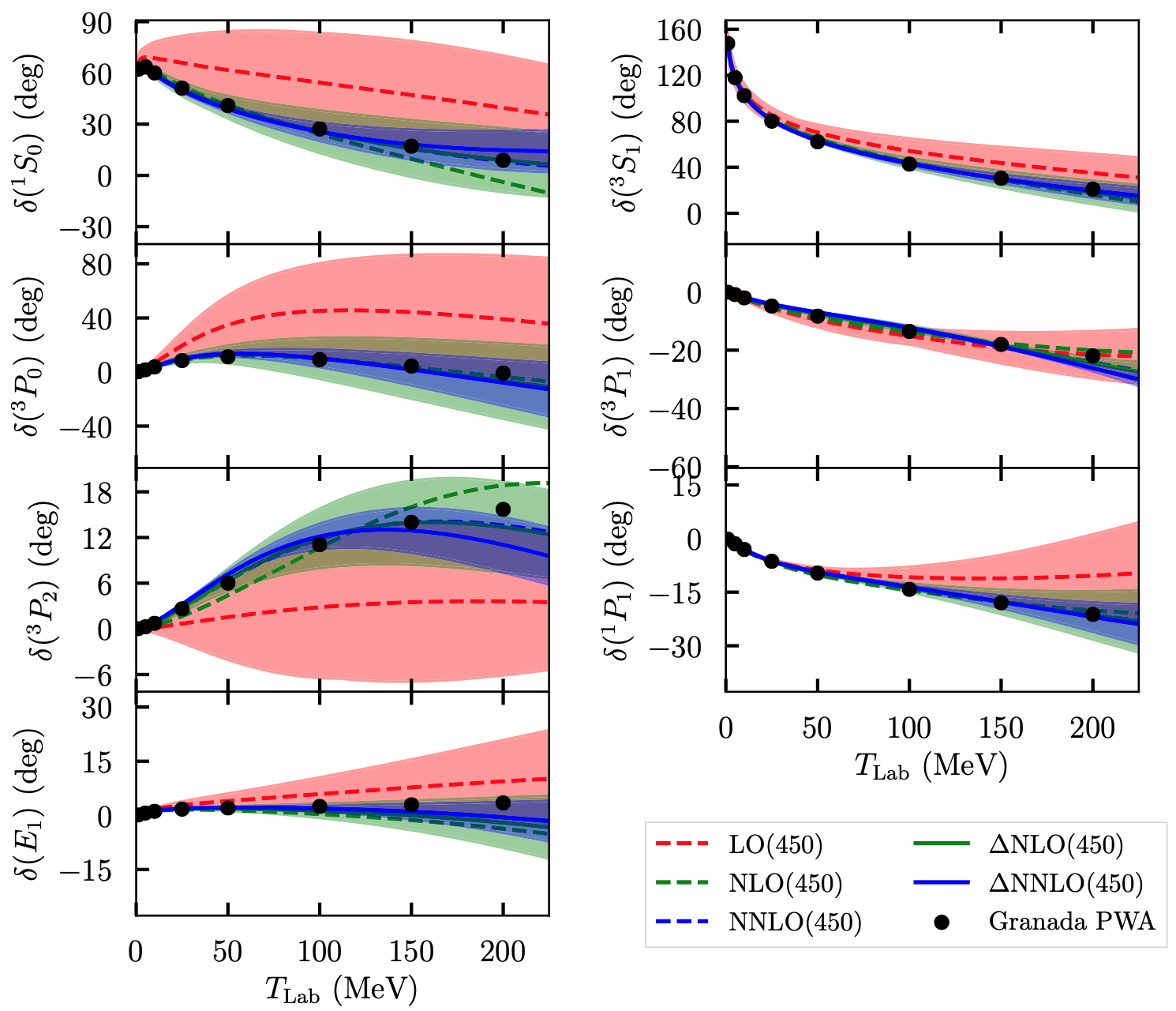
Figure 3: Neutron-proton scattering phase shifts computed with models based on $\Delta$-full and $\Delta$-less chiral interaction potentials. The bands indicate the limits of the expected DOB intervals at each chiral order $\nu$. The black dots represent the values from the Granada partial wave analysis [71].

The procedure for estimating the EFT truncation error, i.e. part of the model discrepancy, requires an estimate of the high-energy scale $\Lambda_{b}$ of the underlying EFT. For the models discussed here, the results are based on chiral EFT, for which the naive estimate of $\Lambda_{b}$ is roughly $M_{N}\sim$1 GeV. This was analyzed more carefully for semi-local chiral potentials [104, 103] in Ref. [105]. The posterior pdf for $\Lambda_{b}$ indicated that a more probable value is $\Lambda_{b}\approx 500$ MeV. This value was also used for the breakdown scale in the truncation error analysis of nucleon-nucleon scattering phase shifts from the $\Delta$-full models at LO,NLO, and NNLO chiral orders in Ref. [93]. The results are presented in Fig. 3. This result also strengthens the observation made earlier, that the inclusion of the $\Delta$ degree of freedom tend to improve model descriptions of nuclear systems. This is more clearly seen when employing the same potentials to make model predictions for the ground-state-energies and charge radii of selected finite nuclei, see Fig. 4, and the energy per nucleon in symmetric nuclear matter, see Fig. 5.

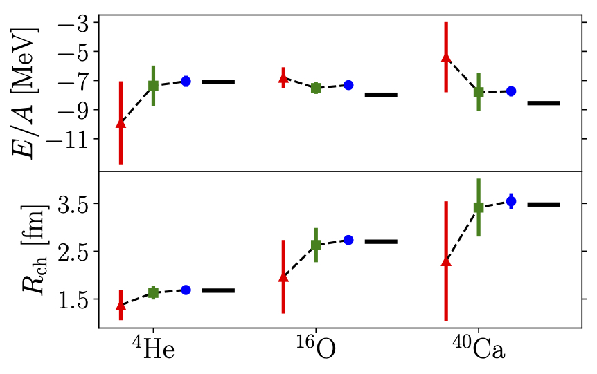
Figure 4: Ground-state energy (negative of binding energy) per nucleon and charge radii for selected nuclei computed with coupled cluster theory and the $\Delta$-full potential $\Delta$NNLO(450). For each nucleus, from left to right as follows: LO (red triangle), NLO (green square), and NNLO (blue circle). The black horizontal bars are data. Vertical bars estimate uncertainties from the order-by-order EFT truncation errors.

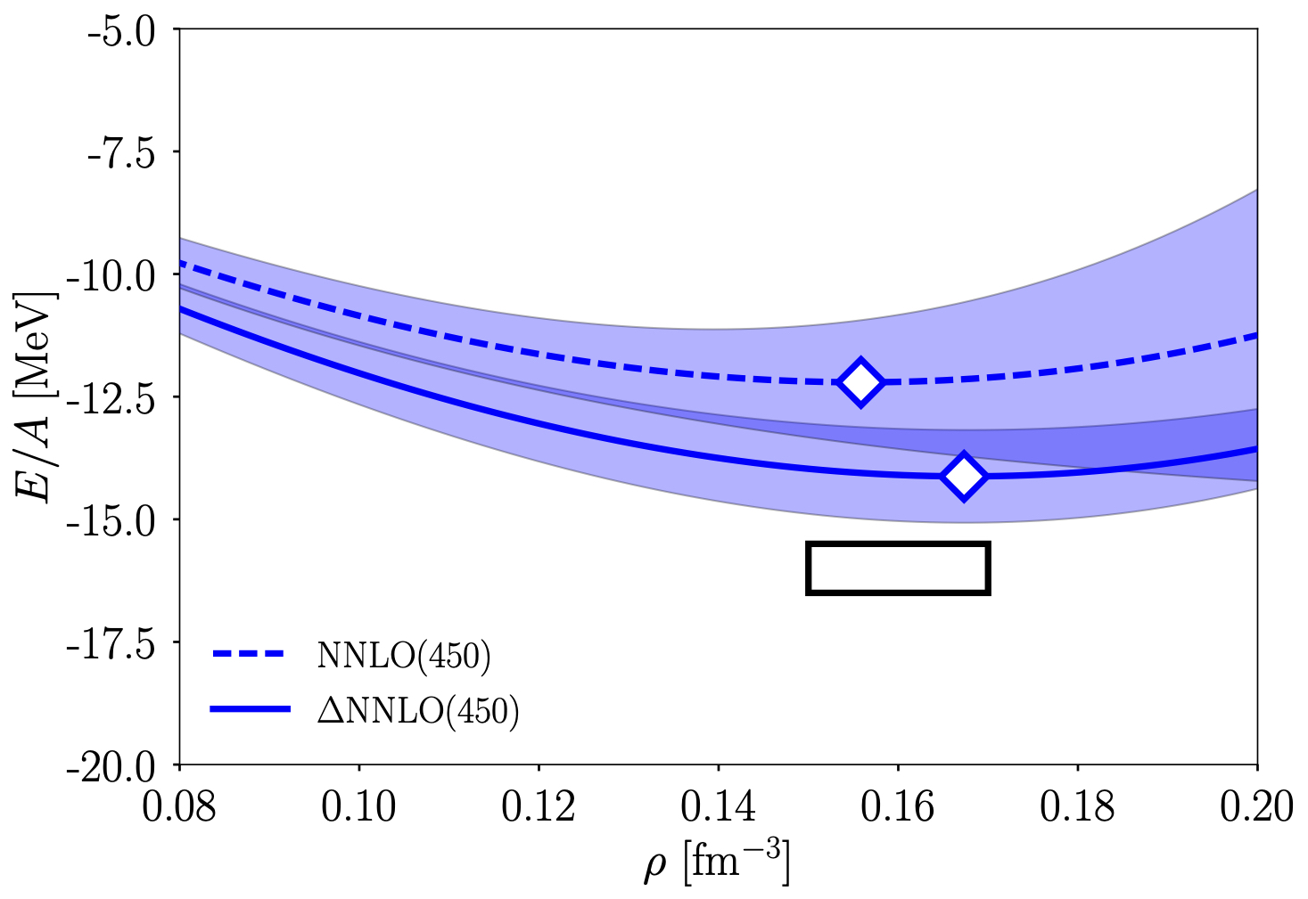
Figure 5: Coupled-cluster based model prediction of the energy per nucleon (in MeV) in symmetric nuclear matter using an NNLO potential with (solid line) and without (dashed line) the $\Delta$ isobar. Both interactions employ a momentum regulator-cutoff $\Lambda$ = 450 MeV. The shaded areas indicate the estimated EFT-truncation errors. The diamonds mark the saturation point and the black rectangle indicates the region $E/A$ = -16 $\pm$ 0.5 MeV and $\rho$ = 0.16 $\pm$ 0.01 fm^-3.

The model predictions for the nuclear matter indicate that the $\Delta$-full models on average agree better with experimental energies and radii. The uncertainty bands for the predictions were extracted under the additional assumption that the relevant soft-scales for finite and infinite nuclear systems are given by the pion mass and the Fermi momentum, respectively. Although these are rough estimates of the soft scales, it is important to note that the the truncation error in Eq. 20 only holds up to factors of order unity. A comparison of theoretical error estimates based on different statistical methods provide additional validation. The Bayesian method for estimating the truncation error and the model errors estimated using the modified $\chi^{2}$-function in Eq. 10 are quite different in nature. Nevertheless, a comparison of the theoretical errors in nucleon-nucleon cross sections at high scattering-energies agree very well for these methods [67, 102]. The link between the two approaches for estimating the model uncertainties is discussed further in Ref. [100]. A complete Bayesian parameter estimation including model discrepancy will hopefully reveal more details about the structure of the chiral EFT error.

At the moment, most model discrepancies in ab initio modelling based on chiral EFT are extracted a posteriori using predictions based on calibrated models. This is possible based on the expectation that the predictions might follow an EFT pattern. This of course remains to be validated on theoretical grounds. However, under the assumption that the interaction potential actually gives rise to an EFT pattern for the observable, we can build on Eq. 4 to include a discrepancy term in the likelihood for calibrating ab initio models. See Ref. [106] for a discussion about correlated truncation errors in nucleon-nucleon scattering observables following this line of thought, where it is also observed that the expansion parameters behave largely as expected.

6 Summary and outlook

Statistical representation of a sound model discrepancy term is certainly challenging. Still, the assumption of zero model discrepancy is a rather extreme position. Almost any reasonable guess is better than nothing in order to avoid false values for the model parameters and to minimize over-fitting.

The importance of model discrepancies is neatly summarized in the famous quote of George E. P. Box: ‘Essentially, all models are wrong, but some are useful’ [107], with the additional comment in Ref. [78]: ’But a model that is wrong can only be useful if we acknowledge the fact that it is wrong.’

Fortunately,most of the ab initio models of atomic nuclei are built on methods from EFT, which by construction promises extra information about the expected impact of the neglected or missing physics in theoretical predictions. Bayesian inference is a natural choice for accounting for model discrepancies and prior knowledge, especially when the priors have a physical basis. Indeed, extracting the posterior pdf for the model parameters via Bayesian inference methods makes it possible to abandon the notion of having a single parameterization of a particular interaction potential and instead build models based on a continuous pdf of parameters. Developments along these lines are already taking place in e.g. density functional theory for atomic nuclei [108].

At the moment, most theoretical analyses of atomic nuclei proceed in the following fashion. Given a potential $V(\vec{\alpha}_{\star})$, optimized to reproduce some set of calibration data $D$, we setup a model $M(\vec{\alpha}_{\star},\vec{x})$ to analyze an experimental result corresponding to the control setting $\vec{x}_{i}$, i.e. we evaluate $M(\vec{\alpha}_{\star},\vec{x}_{i})$. In a few cases we propagate uncertainties originating from the measurement errors present in the data vector $D$, and sometimes we estimate the EFT truncation error using a series of models at different chiral orders. This takes a lot of effort. Indeed, ab initio nuclear models are represented by complex computer codes, implemented via years of dedicated work by several people, and computationally expensive to evaluate. On top of that, to understand the underlying nuclear interaction is, arguably, on of the most difficult problems in all physics. Still, we would like to to answer questions like: how much should we trust a model prediction? is the model $M$ over-fitted? why is it not agreeing with observed data, and how do we understand this discrepancy?

We should strive to use Bayesian methods for calibrating our models $M(\vec{\alpha},\vec{x})$ to obtain posterior pdfs $P(\vec{\alpha}|M,D,I)$ for the parameters. Subsequent evaluations of an observable $\mathcal{O}_{i}$, corresponding to setting the model control variable to $\vec{x}_{i}$, should be marginalized over the parameter posterior pdf to produce a posterior predictive pdf

$$P(\mathcal{O}_{i}|M,\vec{x}_{i},D)=\int{\rm d}\vec{\alpha}\,\,P(\mathcal{O}_{i}|\vec{\alpha},M,\vec{x}_{i},D)P(\vec{\alpha}|M,D).$$ (21)

This quantity will best reflect our state of knowledge, and is quite meaningful to compare with data. Various marginalizations with respect to subsets of the parameters can provide better insights into the qualities of the ab initio model. Bayesian inference also allows us to compare different models via the computation of Bayes factors [109], which in turn enables us to address questions like: which PC in chiral EFT has the strongest support by data? It is also theoretically straightforward to compute the posterior predictive pdf averaged over a set of different models $\mathcal{M}=[M_{1},M_{2},\ldots,M_{3}]$ [110], each weighted by their probability of being true, in the finite space spanned by $\mathcal{M}$, given data $D$.

6.1 The computational challenge

There are several challenges connected with the outlook presented above: working out the theoretical underpinnings of chiral EFT, specifying prior information, formulating model discrepancy terms, and performing challenging Markov Chain Monte Carlo evaluation [111] of complicated posterior pdfs. From a practical point of view, the computational complexity is the most difficult one. Indeed, evaluating models of medium- and heavy-mass atomic nuclei typically requires vast high-performance computing resources. This clearly puts the feasibility of the Bayesian scenario presented above into question. Without any unforeseen disruptive computer technologies or dramatic algorithmic advances, it will be necessary to employ, where possible, fast emulators that accurately mimic the response of the original ab initio models. This is where we can draw from advances in machine learning. Possibly useful methods are e.g. Gaussian process regression and artificial neural networks. Both of these approaches can be challenging since they introduce hyperparameters that require additional optimization. Although it can be difficult to assess how well such methods will work, there exist several examples of useful surrogate interpolation and extrapolation in nuclear modelling, see e.g. Refs. [112, 106, 113, 114, 115, 108, 116]. Recently, a new method called eigenvector continuation [117] turns out to be a promising tool for accurate extrapolation and fast emulation of nuclear properties [118]. In a recent paper [119], this method proved capable of emulating, with a root mean squared error of 1%, more than one million solutions of an ab initio model for the ground-state energy and radius of ¹⁶O in one hour on a standard laptop. An equivalent set of exact ab initio coupled-cluster computations would require 20 years.

Funding

This work was supported by the European Research Council (ERC) under the European Unions Horizon 2020 research and innovation programme (Grant agreement No. 758027).

References

- Dickhoff and Barbieri [2004] Dickhoff WH, Barbieri C. Self-consistent green’s function method for nuclei and nuclear matter. Prog. Part. Nucl. Phys. 52 (2004) 377 – 496. 10.1016/j.ppnp.2004.02.038.
- Lee [2009] Lee D. Lattice simulations for few- and many-body systems. Progress in Particle and Nuclear Physics 63 (2009) 117 – 154. 10.1016/j.ppnp.2008.12.001.
- Bogner et al. [2010] Bogner SK, Furnstahl RJ, Schwenk A. From low-momentum interactions to nuclear structure. Prog. Part. Nucl. Phys. 65 (2010) 94 – 147. 10.1016/j.ppnp.2010.03.001.
- Barrett et al. [2013] Barrett BR, Navrátil P, Vary JP. Ab initio no core shell model. Prog. Part. Nucl. Phys. 69 (2013) 131 – 181. 10.1016/j.ppnp.2012.10.003.
- Carbone et al. [2013] Carbone A, Cipollone A, Barbieri C, Rios A, Polls A. Self-consistent Green’s functions formalism with three-body interactions. Phys. Rev. C 88 (2013) 054326. 10.1103/PhysRevC.88.054326.
- Hagen et al. [2014] Hagen G, Papenbrock T, Hjorth-Jensen M, Dean DJ. Coupled-cluster computations of atomic nuclei. Rep. Prog. Phys. 77 (2014) 096302. 10.1088/0034-4885/77/9/096302.
- Hergert et al. [2014] Hergert H, Bogner SK, Morris TD, Binder S, Calci A, Langhammer J, et al. Ab initio multireference in-medium similarity renormalization group calculations of even calcium and nickel isotopes. Phys. Rev. C 90 (2014) 041302. 10.1103/PhysRevC.90.041302.
- Wiringa et al. [1995] Wiringa RB, Stoks VGJ, Schiavilla R. Accurate nucleon-nucleon potential with charge-independence breaking. Phys. Rev. C 51 (1995) 38–51. 10.1103/PhysRevC.51.38.
- Machleidt [2001] Machleidt R. High-precision, charge-dependent Bonn nucleon-nucleon potential. Phys. Rev. C 63 (2001) 024001. 10.1103/PhysRevC.63.024001.
- Entem and Machleidt [2003] Entem DR, Machleidt R. Accurate charge-dependent nucleon-nucleon potential at fourth order of chiral perturbation theory. Phys. Rev. C 68 (2003) 041001. 10.1103/PhysRevC.68.041001.
- Kolck [1999] Kolck UV. Effective field theory of nuclear forces. Prog. Part. Nucl. Phys. 43 (1999) 337 – 418. 10.1016/S0146-6410(99)00097-6.
- Epelbaum et al. [2009] Epelbaum E, Hammer HW, Meißner UG. Modern theory of nuclear forces. Rev. Mod. Phys. 81 (2009) 1773–1825. 10.1103/RevModPhys.81.1773.
- Machleidt and Entem [2011] Machleidt R, Entem DR. Chiral effective field theory and nuclear forces. Phys. Rep. 503 (2011) 1 – 75. 10.1016/j.physrep.2011.02.001.
- Machleidt [1989] Machleidt R. The Meson Theory of Nuclear Forces and Nuclear Structure (Boston, MA: Springer US), chap. 2 (1989), 189–376. 10.1007/978-1-4613-9907-0_2.
- Elhatisari et al. [2015] Elhatisari S, Lee D, Rupak G, Epelbaum E, Krebs H, Lähde TA, et al. Ab initio alpha–alpha scattering. Nature 528 (2015) 111–114. 10.1038/nature16067.
- Rosenbusch et al. [2015] Rosenbusch M, Ascher P, Atanasov D, Barbieri C, Beck D, Blaum K, et al. Probing the shell closure below the magic proton number : Mass measurements of the exotic isotopes . Phys. Rev. Lett. 114 (2015) 202501. 10.1103/PhysRevLett.114.202501.
- Lapoux et al. [2016] Lapoux V, Somà V, Barbieri C, Hergert H, Holt JD, Stroberg SR. Radii and binding energies in oxygen isotopes: A challenge for nuclear forces. Phys. Rev. Lett. 117 (2016) 052501. 10.1103/PhysRevLett.117.052501.
- Lu et al. [2019] Lu BN, Li N, Elhatisari S, Lee D, Epelbaum E, Meißner UG. Essential elements for nuclear binding. Physics Letters B 797 (2019) 134863. https://doi.org/10.1016/j.physletb.2019.134863.
- Taniuchi et al. [2019] Taniuchi R, Santamaria C, Doornenbal P, Obertelli A, Yoneda K, Authelet G, et al. 78Ni revealed as a doubly magic stronghold against nuclear deformation. Nature 569 (2019) 53–58. 10.1038/s41586-019-1155-x.
- Gysbers et al. [2019] Gysbers P, Hagen G, Holt JD, Jansen GR, Morris TD, Navrátil P, et al. Discrepancy between experimental and theoretical b-decay rates resolved from first principles. Nature Physics (2019). 10.1038/s41567-019-0450-7.
- Somà et al. [2019] Somà V, Navrátil P, Raimondi F, Barbieri C, Duguet T. Novel chiral Hamiltonian and observables in light and medium-mass nuclei. arXiv e-prints (2019) arXiv:1907.09790.
- Binder et al. [2014] Binder S, Langhammer J, Calci A, Roth R. Ab initio path to heavy nuclei. Physics Letters B 736 (2014) 119 – 123. https://doi.org/10.1016/j.physletb.2014.07.010.
- Ekström et al. [2015] Ekström A, Jansen GR, Wendt KA, Hagen G, Papenbrock T, Carlsson BD, et al. Accurate nuclear radii and binding energies from a chiral interaction. Phys. Rev. C 91 (2015) 051301. 10.1103/PhysRevC.91.051301.
- Hagen et al. [2016] Hagen G, Ekström A, Forssén C, Jansen GR, Nazarewicz W, Papenbrock T, et al. Neutron and weak-charge distributions of the 48Ca nucleus. Nature Phys. 12 (2016) 186. 10.1038/nphys3529.
- Garcia Ruiz et al. [2016] Garcia Ruiz RF, Bissell ML, Blaum K, Ekström A, Frömmgen N, Hagen G, et al. Unexpectedly large charge radii of neutron-rich calcium isotopes. Nature Physics (2016). 10.1038/nphys3645.
- Duguet et al. [2017] Duguet T, Somà V, Lecluse S, Barbieri C, Navrátil P. Ab initio calculation of the potential bubble nucleus 34Si. Phys. Rev. C 95 (2017) 034319. 10.1103/PhysRevC.95.034319.
- Nogga et al. [2004] Nogga A, Bogner SK, Schwenk A. Low-momentum interaction in few-nucleon systems. Phys. Rev. C 70 (2004) 061002. 10.1103/PhysRevC.70.061002.
- Hebeler et al. [2011] Hebeler K, Bogner SK, Furnstahl RJ, Nogga A, Schwenk A. Improved nuclear matter calculations from chiral low-momentum interactions. Phys. Rev. C 83 (2011) 031301. 10.1103/PhysRevC.83.031301.
- Hagen et al. [2016] Hagen G, Jansen GR, Papenbrock T. Structure of from first-principles computations. Phys. Rev. Lett. 117 (2016) 172501. 10.1103/PhysRevLett.117.172501.
- Morris et al. [2018] Morris TD, Simonis J, Stroberg SR, Stumpf C, Hagen G, Holt JD, et al. Structure of the lightest tin isotopes. Phys. Rev. Lett. 120 (2018) 152503. 10.1103/PhysRevLett.120.152503.
- Simonis et al. [2017] Simonis J, Stroberg SR, Hebeler K, Holt JD, Schwenk A. Saturation with chiral interactions and consequences for finite nuclei. Phys. Rev. C 96 (2017) 014303. 10.1103/PhysRevC.96.014303.
- Liu et al. [2019] Liu HN, Obertelli A, Doornenbal P, Bertulani CA, Hagen G, Holt JD, et al. How robust is the subshell closure? first spectroscopy of . Phys. Rev. Lett. 122 (2019) 072502. 10.1103/PhysRevLett.122.072502.
- Holt et al. [2019] Holt JD, Stroberg SR, Schwenk A, Simonis J. Ab initio limits of atomic nuclei. arXiv e-prints (2019) arXiv:1905.10475.
- Ireland and Nazarewicz [2015] Ireland DG, Nazarewicz W. Enhancing the interaction between nuclear experiment and theory through information and statistics. Journal of Physics G: Nuclear and Particle Physics 42 (2015) 030301. 10.1088/0954-3899/42/3/030301.
- Hartmann [2001] Hartmann S. Effective field theories, reductionism and scientific explanation. Studies in History and Philosophy of Science Part B: Studies in History and Philosophy of Modern Physics 32 (2001) 267 – 304. https://doi.org/10.1016/S1355-2198(01)00005-3. Spacetime, Fields and Understanding: Persepectives on Quantum Field.
- Barnea et al. [2015] Barnea N, Contessi L, Gazit D, Pederiva F, van Kolck U. Effective field theory for lattice nuclei. Phys. Rev. Lett. 114 (2015) 052501. 10.1103/PhysRevLett.114.052501.
- Chang et al. [2018] Chang CC, Nicholson AN, Rinaldi E, Berkowitz E, Garron N, Brantley DA, et al. A per-cent-level determination of the nucleon axial coupling from quantum chromodynamics. Nature Publishing Group 558 (2018) 91–94.
- Weinberg [1979] Weinberg S. Phenomenological lagrangians. Physica A: Statistical Mechanics and its Applications 96 (1979) 327 – 340. https://doi.org/10.1016/0378-4371(79)90223-1.
- Weinberg [1990] Weinberg S. Nuclear forces from chiral lagrangians. Phys. Lett. B 251 (1990) 288 – 292. 10.1016/0370-2693(90)90938-3.
- Bedaque and van Kolck [2002] Bedaque PF, van Kolck U. Effective field theory for few-nucleon systems. Annual Review of Nuclear and Particle Science 52 (2002) 339–396. 10.1146/annurev.nucl.52.050102.090637.
- Papenbrock [2011] Papenbrock T. Effective theory for deformed nuclei. Nuclear Physics A 852 (2011) 36 – 60. https://doi.org/10.1016/j.nuclphysa.2010.12.013.
- Gasser and Leutwyler [1984] Gasser J, Leutwyler H. Chiral perturbation theory to one loop. Annals of Physics 158 (1984) 142 – 210. https://doi.org/10.1016/0003-4916(84)90242-2.
- van Kolck [1994] van Kolck U. Few-nucleon forces from chiral Lagrangians. Phys. Rev. C 49 (1994) 2932–2941. 10.1103/PhysRevC.49.2932.
- Epelbaum et al. [2002] Epelbaum E, Nogga A, Glöckle W, Kamada H, Meißner UG, Witała H. Three-nucleon forces from chiral effective field theory. Phys. Rev. C 66 (2002) 064001. 10.1103/PhysRevC.66.064001.
- Bernard et al. [2008] Bernard V, Epelbaum E, Krebs H, Meißner UG. Subleading contributions to the chiral three-nucleon force: Long-range terms. Phys. Rev. C 77 (2008) 064004. 10.1103/PhysRevC.77.064004.
- Bernard et al. [2011] Bernard V, Epelbaum E, Krebs H, Meißner UG. Subleading contributions to the chiral three-nucleon force. ii. short-range terms and relativistic corrections. Phys. Rev. C 84 (2011) 054001. 10.1103/PhysRevC.84.054001.
- Park et al. [1993] Park TS, Min DP, Rho M. Chiral dynamics and heavy-fermion formalism in nuclei: exchange axial currents. Physics Reports 233 (1993) 341 – 395. https://doi.org/10.1016/0370-1573(93)90099-Y.
- Park et al. [1996] Park TS, Min DP, Rho M. Chiral lagrangian approach to exchange vector currents in nuclei. Nuclear Physics A 596 (1996) 515 – 552. https://doi.org/10.1016/0375-9474(95)00406-8.
- Krebs et al. [2017] Krebs H, Epelbaum E, Meißner UG. Nuclear axial current operators to fourth order in chiral effective field theory. Annals of Physics 378 (2017) 317 – 395. https://doi.org/10.1016/j.aop.2017.01.021.
- Baroni et al. [2016] Baroni A, Girlanda L, Pastore S, Schiavilla R, Viviani M. Nuclear axial currents in chiral effective field theory. Phys. Rev. C 93 (2016) 015501. 10.1103/PhysRevC.93.015501.
- Hoferichter et al. [2016] Hoferichter M, de Elvira JR, Kubis B, Meißner UG. Roy-steiner-equation analysis of pion-nucleon scattering. Physics Reports 625 (2016) 1 – 88. https://doi.org/10.1016/j.physrep.2016.02.002. Roy-Steiner-equation analysis of pion-nucleon scattering.
- Lepage [1997] Lepage P. How to renormalize the schrodinger equation. ArXiv e-prints (1997) nucl–th/9706029.
- Grieshammer [2015] Grieshammer H, editor. Assessing Theory Uncertainties in EFT Power Countings from Residual Cutoff Dependence, The 8th International Workshop on Chiral Dynamics, CD2015g, vol. 253 (Proceedings of Science) (2015).
- Nogga et al. [2005] Nogga A, Timmermans RGE, Kolck Uv. Renormalization of one-pion exchange and power counting. Phys. Rev. C 72 (2005) 054006. 10.1103/PhysRevC.72.054006.
- Pavón Valderrama and Arriola [2006] Pavón Valderrama M, Arriola ER. Renormalization of the interaction with a chiral two-pion-exchange potential: Central phases and the deuteron. Phys. Rev. C 74 (2006) 054001. 10.1103/PhysRevC.74.054001.
- Long and Yang [2012] Long B, Yang CJ. Renormalizing chiral nuclear forces: Triplet channels. Phys. Rev. C 85 (2012) 034002. 10.1103/PhysRevC.85.034002.
- Epelbaum and Meißner [2013] Epelbaum E, Meißner UG. On the renormalization of the one–pion exchange potential and the consistency of weinberg’s power counting. Few-Body Systems 54 (2013) 2175–2190. 10.1007/s00601-012-0492-1.
- Dyhdalo et al. [2016] Dyhdalo A, Furnstahl RJ, Hebeler K, Tews I. Regulator artifacts in uniform matter for chiral interactions. Phys. Rev. C 94 (2016) 034001. 10.1103/PhysRevC.94.034001.
- Sánchez et al. [2018] Sánchez MS, Yang CJ, Long B, van Kolck U. Two-nucleon amplitude zero in chiral effective field theory. Phys. Rev. C 97 (2018) 024001. 10.1103/PhysRevC.97.024001.
- Epelbaum et al. [2018] Epelbaum E, Gasparyan AM, Gegelia J, Meißner UG. How (not) to renormalize integral equations with singular potentials in effective field theory. The European Physical Journal A 54 (2018) 186. 10.1140/epja/i2018-12632-1.
- Yang [2019] Yang CJ. Do we know how to count powers in pionless and pionful effective field theory? ArXiv e-prints (2019) 1905.12510.
- Flambaum and Wiringa [2007] Flambaum VV, Wiringa RB. Dependence of nuclear binding on hadronic mass variation. Phys. Rev. C 76 (2007) 054002. 10.1103/PhysRevC.76.054002.
- Epelbaum et al. [2013] Epelbaum E, Krebs H, Lähde TA, Lee D, Meißner UG. Viability of carbon-based life as a function of the light quark mass. Phys. Rev. Lett. 110 (2013) 112502. 10.1103/PhysRevLett.110.112502.
- Kamada et al. [2001] Kamada H, Nogga A, Glöckle W, Hiyama E, Kamimura M, Varga K, et al. Benchmark test calculation of a four-nucleon bound state. Phys. Rev. C 64 (2001) 044001. 10.1103/PhysRevC.64.044001.
- Hebeler et al. [2015] Hebeler K, Holt J, Menéndez J, Schwenk A. Nuclear forces and their impact on neutron-rich nuclei and neutron-rich matter. Annual Review of Nuclear and Particle Science 65 (2015) 457–484. 10.1146/annurev-nucl-102313-025446.
- Hergert [2016] Hergert H. In-medium similarity renormalization group for closed and open-shell nuclei. Physica Scripta 92 (2016) 023002. 10.1088/1402-4896/92/2/023002.
- Carlsson et al. [2016] Carlsson BD, Ekström A, Forssén C, Strömberg DF, Jansen GR, Lilja O, et al. Uncertainty analysis and order-by-order optimization of chiral nuclear interactions. Phys. Rev. X 6 (2016) 011019. 10.1103/PhysRevX.6.011019.
- Piarulli et al. [2015] Piarulli M, Girlanda L, Schiavilla R, Pérez RN, Amaro JE, Arriola ER. Minimally nonlocal nucleon-nucleon potentials with chiral two-pion exchange including resonances. Phys. Rev. C 91 (2015) 024003. 10.1103/PhysRevC.91.024003.
- Reinert et al. [2018] Reinert P, Krebs H, Epelbaum E. Semilocal momentum-space regularized chiral two-nucleon potentials up to fifth order. The European Physical Journal A 54 (2018) 86. 10.1140/epja/i2018-12516-4.
- Stoks et al. [1993] Stoks VGJ, Klomp RAM, Rentmeester MCM, de Swart JJ. Partial-wave analysis of all nucleon-nucleon scattering data below 350 mev. Phys. Rev. C 48 (1993) 792–815. 10.1103/PhysRevC.48.792.
- Pérez et al. [2013] Pérez RN, Amaro JE, Arriola ER. Coarse-grained potential analysis of neutron-proton and proton-proton scattering below the pion production threshold. Phys. Rev. C 88 (2013) 064002. 10.1103/PhysRevC.88.064002.
- Wild [2017] Wild SM. Solving derivative-free nonlinear least squares problems with POUNDERS. Terlaky T, Anjos MF, Ahmed S, editors, Advances and Trends in Optimization with Engineering Applications (SIAM) (2017), 529–540. 10.1137/1.9781611974683.ch40.
- Ekström et al. [2013] Ekström A, Baardsen G, Forssén C, Hagen G, Hjorth-Jensen M, Jansen GR, et al. Optimized chiral nucleon-nucleon interaction at next-to-next-to-leading order. Phys. Rev. Lett. 110 (2013) 192502. 10.1103/PhysRevLett.110.192502.
- Bergervoet et al. [1988] Bergervoet JR, van Campen PC, van der Sanden WA, de Swart JJ. Phase shift analysis of 0–30 mev pp scattering data. Phys. Rev. C 38 (1988) 15–50. 10.1103/PhysRevC.38.15.
- Tjon [1975] Tjon J. Bound states of 4he with local interactions. Physics Letters B 56 (1975) 217 – 220. https://doi.org/10.1016/0370-2693(75)90378-0.
- Gazit et al. [2009] Gazit D, Quaglioni S, Navrátil P. Three-nucleon low-energy constants from the consistency of interactions and currents in chiral effective field theory. Phys. Rev. Lett. 103 (2009) 102502. 10.1103/PhysRevLett.103.102502.
- Epelbaum et al. [2019] Epelbaum E, Golak J, Hebeler K, Hüther T, Kamada H, Krebs H, et al. Few- and many-nucleon systems with semilocal coordinate-space regularized chiral two- and three-body forces. Phys. Rev. C 99 (2019) 024313. 10.1103/PhysRevC.99.024313.
- Brynjarsdóttir and O’Hagan [2014] Brynjarsdóttir J, O’Hagan A. Learning about physical parameters: the importance of model discrepancy. Inverse Problems 30 (2014) 114007. 10.1088/0266-5611/30/11/114007.
- Andrae et al. [2010] [Dataset] Andrae R, Schulze-Hartung T, Melchior P. Dos and don’ts of reduced chi-squared (2010).
- Furnstahl et al. [2015a] Furnstahl RJ, Phillips DR, Wesolowski S. A recipe for EFT uncertainty quantification in nuclear physics. Journal of Physics G: Nuclear and Particle Physics 42 (2015a) 034028. 10.1088/0954-3899/42/3/034028.
- Dobaczewski et al. [2014] Dobaczewski J, Nazarewicz W, Reinhard PG. Error estimates of theoretical models: a guide. Journal of Physics G: Nuclear and Particle Physics 41 (2014) 074001. 10.1088/0954-3899/41/7/074001.
- Ekström et al. [2015] Ekström A, Carlsson BD, Wendt KA, Forssén C, Jensen MH, Machleidt R, et al. Statistical uncertainties of a chiral interaction at next-to-next-to leading order. J. Phys. G 42 (2015) 034003. 10.1088/0954-3899/42/3/034003.
- Navarro Pérez et al. [2015] Navarro Pérez R, Amaro JE, Ruiz Arriola E, Maris P, Vary JP. Statistical error propagation in ab initio no-core full configuration calculations of light nuclei. Phys. Rev. C 92 (2015) 064003. 10.1103/PhysRevC.92.064003.
- Navarro Pérez et al. [2014] Navarro Pérez R, Amaro JE, Ruiz Arriola E. Statistical error analysis for phenomenological nucleon-nucleon potentials. Phys. Rev. C 89 (2014) 064006. 10.1103/PhysRevC.89.064006.
- Acharya et al. [2016] Acharya B, Carlsson B, Ekstr̦m A, Forss̩n C, Platter L. Uncertainty quantification for proton-proton fusion in chiral effective field theory. Physics Letters B 760 (2016) 584 Р589. https://doi.org/10.1016/j.physletb.2016.07.032.
- Acharya et al. [2018] Acharya B, Ekström A, Platter L. Effective-field-theory predictions of the muon-deuteron capture rate. Phys. Rev. C 98 (2018) 065506. 10.1103/PhysRevC.98.065506.
- Hernandez et al. [2018] Hernandez O, Ekstr̦m A, Dinur NN, Ji C, Bacca S, Barnea N. The deuteron-radius puzzle is alive: A new analysis of nuclear structure uncertainties. Physics Letters B 778 (2018) 377 Р383. https://doi.org/10.1016/j.physletb.2018.01.043.
- Carlsson [2017] Carlsson BD. Quantifying statistical uncertainties in ab initio nuclear physics using lagrange multipliers. Phys. Rev. C 95 (2017) 034002. 10.1103/PhysRevC.95.034002.
- Rotureau et al. [2018] Rotureau J, Danielewicz P, Hagen G, Jansen GR, Nunes FM. Microscopic optical potentials for calcium isotopes. Phys. Rev. C 98 (2018) 044625. 10.1103/PhysRevC.98.044625.
- Idini et al. [2019] Idini A, Barbieri C, Navrátil P. Ab initio optical potentials and nucleon scattering on medium mass nuclei. Phys. Rev. Lett. 123 (2019) 092501. 10.1103/PhysRevLett.123.092501.
- Elhatisari et al. [2016] Elhatisari S, Li N, Rokash A, Alarcón JM, Du D, Klein N, et al. Nuclear binding near a quantum phase transition. Phys. Rev. Lett. 117 (2016) 132501. 10.1103/PhysRevLett.117.132501.
- Hagen et al. [2016] Hagen G, Hjorth-Jensen M, Jansen GR, Papenbrock T. Emergent properties of nuclei from ab initio coupled-cluster calculations. Phys. Scr. 91 (2016) 063006. 10.1088/0031-8949/91/6/063006.
- Ekström et al. [2018] Ekström A, Hagen G, Morris TD, Papenbrock T, Schwartz PD. isobars and nuclear saturation. Phys. Rev. C 97 (2018) 024332. 10.1103/PhysRevC.97.024332.
- Piarulli et al. [2018] Piarulli M, Baroni A, Girlanda L, Kievsky A, Lovato A, Lusk E, et al. Light-nuclei spectra from chiral dynamics. Phys. Rev. Lett. 120 (2018) 052503. 10.1103/PhysRevLett.120.052503.
- Logoteta et al. [2016] Logoteta D, Bombaci I, Kievsky A. Nuclear matter properties from local chiral interactions with isobar intermediate states. Phys. Rev. C 94 (2016) 064001. 10.1103/PhysRevC.94.064001.
- Kalantar-Nayestanaki et al. [2011] Kalantar-Nayestanaki N, Epelbaum E, Messchendorp JG, Nogga A. Signatures of three-nucleon interactions in few-nucleon systems. Reports on Progress in Physics 75 (2011) 016301. 10.1088/0034-4885/75/1/016301.
- de Finetti [2017] de Finetti B. Theory of Probability: A Critical Introductory Treatment (John Wiley and Sons Ltd.) (2017).
- Schindler and Phillips [2009] Schindler M, Phillips D. Bayesian methods for parameter estimation in effective field theories. Ann. Phys. 324 (2009) 682 – 708. 10.1016/j.aop.2008.09.003.
- Wesolowski et al. [2016] Wesolowski S, Klco N, Furnstahl RJ, Phillips DR, liya AT. Bayesian parameter estimation for effective field theories. Journal of Physics G: Nuclear and Particle Physics 43 (2016) 074001.
- Wesolowski et al. [2019] Wesolowski S, Furnstahl RJ, Melendez JA, Phillips DR. Exploring bayesian parameter estimation for chiral effective field theory using nucleon–nucleon phase shifts. Journal of Physics G: Nuclear and Particle Physics 46 (2019) 045102. 10.1088/1361-6471/aaf5fc.
- Cacciari and Houdeau [2011] Cacciari M, Houdeau N. Meaningful characterisation of perturbative theoretical uncertainties. Journal of High Energy Physics 2011 (2011) 39. 10.1007/JHEP09(2011)039.
- Furnstahl et al. [2015b] Furnstahl RJ, Klco N, Phillips DR, Wesolowski S. Quantifying truncation errors in effective field theory. Phys. Rev. C 92 (2015b) 024005. 10.1103/PhysRevC.92.024005.
- Epelbaum et al. [2015a] Epelbaum E, Krebs H, Meißner UG. Improved chiral nucleon-nucleon potential up to next-to-next-to-next-to-leading order. The European Physical Journal A 51 (2015a) 53. 10.1140/epja/i2015-15053-8.
- Epelbaum et al. [2015b] Epelbaum E, Krebs H, Meißner UG. Precision nucleon-nucleon potential at fifth order in the chiral expansion. Phys. Rev. Lett. 115 (2015b) 122301. 10.1103/PhysRevLett.115.122301.
- Melendez et al. [2017] Melendez JA, Wesolowski S, Furnstahl RJ. Bayesian truncation errors in chiral effective field theory: Nucleon-nucleon observables. Phys. Rev. C 96 (2017) 024003. 10.1103/PhysRevC.96.024003.
- Melendez et al. [2019] Melendez JA, Furnstahl RJ, Phillips DR, Pratola MT, Wesolowski S. Quantifying correlated truncation errors in effective field theory. Phys. Rev. C 100 (2019) 044001. 10.1103/PhysRevC.100.044001.
- Box and Draper [1987] Box GE, Draper NR. Empirical model-building and response surfaces. (John Wiley & Sons) (1987).
- Neufcourt et al. [2019] Neufcourt L, Cao Y, Nazarewicz W, Olsen E, Viens F. Neutron drip line in the ca region from bayesian model averaging. Phys. Rev. Lett. 122 (2019) 062502. 10.1103/PhysRevLett.122.062502.
- Gelman et al. [2013] Gelman A, Carlin JB, Stern HS, Dunson DB, Vehtari A, Rubin DB. Bayesian Data Analysis, Third Edition. Chapman Hall/CRC Texts in Statistical Science (Taylor Francis) (2013).
- Hoeting et al. [1999] Hoeting JA, Madigan D, Raftery AE, Volinsky CT. Bayesian model averaging: A tutorial. Statistical Science 14 (1999) 382–401.
- Brooks et al. [2011] Brooks S, Gelman A, Jones G, Meng XL. Handbook of Markov Chain Monte Carlo (CRC press) (2011).
- Ekström et al. [2019] Ekström A, Forssén C, Dimitrakakis C, Dubhashi D, Johansson HT, Muhammad AS, et al. Bayesian optimization in ab initio nuclear physics. Journal of Physics G: Nuclear and Particle Physics 46 (2019) 095101. 10.1088/1361-6471/ab2b14.
- Negoita et al. [2019] Negoita GA, Vary JP, Luecke GR, Maris P, Shirokov AM, Shin IJ, et al. Deep learning: Extrapolation tool for ab initio nuclear theory. Phys. Rev. C 99 (2019) 054308. 10.1103/PhysRevC.99.054308.
- Jiang et al. [2019] Jiang WG, Hagen G, Papenbrock T. Extrapolation of nuclear structure observables with artificial neural networks. Phys. Rev. C 100 (2019) 054326. 10.1103/PhysRevC.100.054326.
- Neufcourt et al. [2018] Neufcourt L, Cao Y, Nazarewicz W, Viens F. Bayesian approach to model-based extrapolation of nuclear observables. Phys. Rev. C 98 (2018) 034318. 10.1103/PhysRevC.98.034318.
- McDonnell et al. [2015] McDonnell JD, Schunck N, Higdon D, Sarich J, Wild SM, Nazarewicz W. Uncertainty quantification for nuclear density functional theory and information content of new measurements. Phys. Rev. Lett. 114 (2015) 122501. 10.1103/PhysRevLett.114.122501.
- Frame et al. [2018] Frame D, He R, Ipsen I, Lee D, Lee D, Rrapaj E. Eigenvector continuation with subspace learning. Phys. Rev. Lett. 121 (2018) 032501. 10.1103/PhysRevLett.121.032501.
- König et al. [2019] König S, Ekström A, Hebeler K, Lee D, Schwenk A. Eigenvector Continuation as an Efficient and Accurate Emulator for Uncertainty Quantification. arXiv e-prints (2019) arXiv:1909.08446.
- Ekström and Hagen [2019] Ekström A, Hagen G. Global sensitivity analysis of bulk properties of an atomic nucleus. ArXiv e-prints (2019) 1910.02922.