Channel Estimation, Interference Cancellation, and Symbol Detection for Communications on Overlapping Channels

Abstract

In this paper, we propose the joint interference cancellation, fast fading channel estimation, and data symbol detection for a general interference setting where the interfering source and the interfered receiver are unsynchronized and occupy overlapping channels of different bandwidths. The interference must be canceled before the channel estimation and data symbol detection of the desired communication are performed. To this end, we have to estimate the Effective Interference Coefficients (EICs) and then the desired fast fading channel coefficients. We construct a two-phase framework where the EICs and desired channel coefficients are estimated using the joint maximum likelihood-maximum a posteriori probability (JML-MAP) criteria in the first phase; and the MAP based data symbol detection is performed in the second phase. Based on this two-phase framework, we also propose an iterative algorithm for interference cancellation, channel estimation and data detection. We analyze the channel estimation error, residual interference, symbol error rate (SER) achieved by the proposed framework. We then discuss how to optimize the pilot density to achieve the maximum throughput. Via numerical studies, we show that our design can effectively mitigate the interference for a wide range of SNR values, our proposed channel estimation and symbol detection design can achieve better performances compared to the existing method. Moreover, we demonstrate the improved performance of the iterative algorithm with respect to the non-iterative counterpart.

I Introduction

Traffic demand from wireless networks has been increasing dramatically over the last decades while the spectrum resource is limited. This has motivated the development of efficient and flexible spectrum utilization and sharing techniques. Moreover, future wireless networks are expected to support a massive number of connections to enable many emerging applications requiring diverse communication rates and qualities of service [1]. Therefore, effective spectrum reuses using robust interference cancellation and management are essential in maintaining and enhancing the communication rates and reliability in next-generation wireless systems [2]. In particular, future wireless systems must be able to support different applications and use cases, e.g., highly mobile scenarios in which users move at high speeds (up to 500 km/hr) [3, 4, 5]. Thus, developing wireless communication techniques for high mobility environments is of high importance and has attracted increasing research attention [6, 7, 8].

Non-Orthogonal Multiple Access (NOMA) [9] and Full Duplex (FD) communication [10] are among the advanced frequency reuse techniques. In NOMA, signals from different sources are allowed to be transmitted simultaneously over the same channel, and successive interference cancellation is typically employed to decode these messages. Moreover, a FD transceiver allows to transmit and receive at the same time over the same channel, thus, the receiver experiences severe self-interference from the transmitter. As a result, advanced interference cancellation techniques are required to realize a practical FD system where combined analog and digital interference cancellation strategies are usually employed to achieve sufficient cancellation performance [11].

Note, however, that FD communication has a special interference structure where the interfering and interfered communications have the same bandwidth (hence, the same symbol rate). This interference structure plays a crucial role in designing interference cancellation techniques, especially in the digital domain [12, 13]. Interference cancellation in the more general scenario where the interfering source and victim have different bandwidths is more challenging to tackle because of the following reasons. First, the equivalent interference coefficients (EIC) [14] vary from symbol to symbol and they are difficult to capture. Second, when operating over different bandwidths, these concurrent communications are likely not synchronized, which creates a fundamental limitation in cancellation performance [15].

Various interference cancellation techniques, including passive interference cancellations [16], active interference cancellations in the analog domain [17, 18] and in the digital domain [13, 12], have been proposed for full-duplex systems. However, only a few works study interference cancellation for the concurrent communications with different bandwidths even though this interfering scenario can arise in both terrestrial communications [19] and satellite communications [20]. In fact, this interference scenario occurs between the Iridium satellite system operating in the band 1621.35 - 1626.5 MHz and the Inmarsat satellite system operating in the adjacent band 1626.5 - 1660.5 MHz, as reported in [21]. Thus, development of robust interference cancellation methods that effectively address the general interference scenario between two communications of different bandwidths is highly important.

Interference cancellation for communications with different bandwidths has been investigated in some previous works [22, 14] assuming perfect CSI and/or synchronization between the underlying communications. The problem becomes much more challenging when the desired channel experiences the fast fading where the time-varying channel can be modeled by using the Gauss-Markov process [23, 24, 25, 26, 7, 27]. For the fast fading channel, MMSE-based channel estimators are derived in [28, 29] requiring the knowledge of the channel correlation matrix, which may not be readily usable in the presence of interference. Therefore, it is highly desirable to develop robust interference cancellation techniques that can effectively cope with a strong interfering signal with different bandwidth from the victim in the fast fading environment.

Data symbol detection in the fast fading environment is another challenging task, especially with the presence of strong interference. A well-known approach for symbol detection in fast fading environments is the message-passing detection technique in which the posterior probability of data symbols is estimated. In [27], it is shown that this detection technique can function well if the interfering signal has similar characteristics with the desired signal. However, the method works well only if the interfering and desired signals are synchronized and have the same symbol rate. Furthermore, an approximated distribution of data symbols by the Gaussian mixture with a limited number of terms may yield unacceptable error rate with a large signal constellation size. Another approach is considered in [30] where the channel gains at data symbols are interpolated by the imperfect CSI at pilot symbols. Then, the zero-forcing based symbol detection is employed, the technique is called optimum diversity detection (ODD). However, this detection technique does not fully exploit the correlations of channel gains at consecutive data symbols, and the required inverse matrix operations result in high computational complexity. This motivates us to develop a new detection strategy that has low complexity and can achieve the performance close to that of the ODD technique.

The above survey suggests that joint channel estimation, interference cancellation, and symbol detection for the scenario in which two un-synchronized mutual interfering signals have different bandwidths in the fast fading environment has been under-explored. This paper aims to fill this gap in the literature where we make the following contributions.

• Firstly, a two-phase framework for joint interference cancellation, channel estimation, and symbol detection is proposed. In the first phase, the EICs are estimated and the interference is subtracted. Then, fast-fading channel coefficients at pilot positions are estimated. In the second phase, we derive the a posteriori probabilities for both series and individual symbols, given the channel coefficients at pilot positions. Based on these probabilities, we propose corresponding detection methods. Specifically, our series symbol detection (S-MAP) outperforms the existing ODD technique [30] while our individual symbol detection (I-MAP) achieves almost identical result to the ODD technique with much lower complexity as confirmed by numerical studies.

• Secondly, based on the proposed two-phase framework, we propose an iterative algorithm for interference cancellation, channel estimation, and data detection. Numerical studies show that the proposed iterative algorithm converges quite quickly and it performs better than the non-iterative counterpart.

• Thirdly, we analyze the residual interference and symbol error rate achieved by the proposed non-iterative algorithm. Specifically, we provide an exact expression for channel estimation error in the interference-free scenario, and an approximated residual interference and channel estimation error for the case with interference. The analysis shows that the residual interference has bounded power as the interference power tends to infinity. However, the effect of the fast fading channel to the residual interference is irreducible no matter how large the SNR or the number of pilot symbols is. Hence, there are fundamental floors for the channel estimation and symbol detection performances.

• Finally, we conduct simulation studies and draw several insightful observations from the results. Particularly, the performance floor exists for the considered interference scenario while it is not the case for the interference free scenario. It is also shown that the existing symbol detection method may need more than 3dB increment in SNR to achieve the same symbol error rate (SER) obtained from our S-MAP method, while our I-MAP method achieves very close performance to the existing optimum detection method. Finally, we show that there exists an optimal frame structure (i.e., optimal pilot density) to achieve the maximum system throughput.

While preliminary results of this paper were published in [31], the current paper makes several significant contributions compared to this conference version. Specifically, the current journal paper proposes two detection methods with improved performances compared to the method introduced in the conference version. The new iterative algorithm is also proposed in this journal version. The theoretical performance analysis and throughput optimization were not conducted in the conference version. Moreover, the current journal paper presents much more extensive numerical results which provide useful insights into the proposed design.

The paper is structured as follows. The system model and problem formulation are presented in Section II. Section III describes the proposed channel estimation, interference cancellation, and the symbol detection techniques. In Section IV, we analyze the residual interference, SER, and optimal frame design for the fast fading and interference scenario. Numerical results are presented in Section V and Section VI concludes the paper.

Some important notations used in the paper are summarized as follows: $\mathbf{I}_{N}$ represents the $N\times N$ identity matrix, $\mathbf{1}_{M,N}$ is the $M\times N$ all-one matrix, $\mathbf{A}^{H}$ is the Hermitian transpose of matrix $\mathbf{A}$, $x^{*}$ is the conjugate of complex value $x$, $\mathds{1}_{i=j}$ is the indicator function equal to one when $i=j$ and equal to zero otherwise, $const.$ represents a constant independent of the variables of interest, ($\star$) denotes the convolution operation and $(\propto)$ denotes ‘proportional to’.

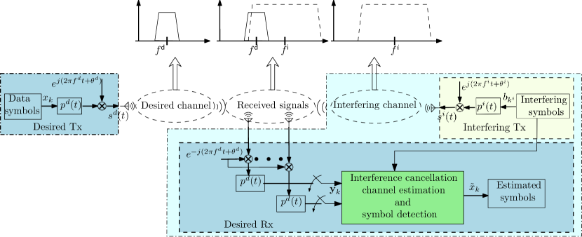
Figure 1: Considered interference scenario

II System Model and Problem Statement

We consider the scenario where two communication links denoted by $\boldsymbol{\mathbb{S}}^{\sf d}$ (desired link) and $\boldsymbol{\mathbb{S}}^{\sf i}$ (interfering link) operate on overlapping frequency bands. The transmitted signal from $\boldsymbol{\mathbb{S}}^{\sf i}$ interferes with the received signal of $\boldsymbol{\mathbb{S}}^{\sf d}$. One popular assumption usually made in the literature is that interfering and desired signals have identical bandwidths where the full-duplex system is a special setting attracting great interests recently. Our current paper considers the more general scenario in which the frequency bands of the two communication links can be arbitrarily aligned and their bandwidth ratio is an integer. The considered setting corresponds to the practical interference scenarios in satellite communications [20, 21] and terrestrial communications, e.g., full-duplex relay [32, 33].

We further assume that the desired communication channel experiences the fast fading where the channel coefficient changes from symbol to symbol according to the first order Markov process [23, 25]. In addition, the interfering channel from the interfering source to the antennas of the desired receiver is assumed to be line of sight. In this interference scenario, the involved signals have different bandwidths and are not synchronized with each other. This induces a dynamic interference pattern to the desired received signal, which can be captured by the EICs [14, 22]. We propose to jointly estimate the desired channel coefficients and the EICs with the knowledge of transmitted symbols from the interfering source and the pilot symbols of the desired signal.

The considered setting with desired and interfering communications is illustrated in Fig. 1. The studied interference scenario occurs in practice when the interfering Tx and the desired Rx are located close to each other and the desired Rx has access to the interfering symbols (e.g., via a dedicated connection) as in the full-duplex relay [32, 33]. More details about the system are introduced in the followings.

II-A Signal Models

The transmitted signal of the desired communication with the carrier frequency $f^{\sf d}$ can be written as

$$s^{\sf d}(t)=\sum_{k=-\infty}^{\infty}{x_{k}p^{\sf d}(t{-}kT^{\sf d}{+}\epsilon^{\sf d})e^{j(2\pi f^{\sf d}t+\theta^{\sf d})}},\\$$ (1)

where $x_{k}$ is the $k$th transmitted symbol. The pulse shaping function $p^{\sf d}(t)$ has unity gain; $T^{\sf d}$, $\epsilon^{\sf d}$ and $\theta^{\sf d}$ represent the symbol duration, time and phase offsets, respectively. Similarly, the signal from the interfering source can be written as

$$s^{\sf i}(t)=\sum_{k^{\sf i}=-\infty}^{\infty}{b_{k^{\sf i}}p^{\sf i}(t{-}k^{\sf i}T^{\sf i}{-}t^{\sf i})e^{j(2\pi f^{\sf i}t+\theta^{\sf i})}},\\$$ (2)

where $p^{\sf i}(t)$ denotes the pulse shaping filter with unity gain, the interfering signal has the center frequency $f^{\sf i}=f^{\sf d}-\Delta f$, the $k^{\sf i}$th symbol is $b_{k^{\sf i}}$; $t^{\sf i}$ and $\theta^{\sf i}$ account for the time/phase difference of the two systems and transmission time delay from the interfering transmitter to the interfered receiver, respectively. Assume that there are $N_{\sf r}$ receiver antennas for $\boldsymbol{\mathbb{S}}^{\sf d}$, then the received signal is

$$\mathbf{y}(t)=\mathbf{h}^{\sf d}(t)\star s^{\sf d}(t)+\mathbf{h}^{\sf i}(t)\star s^{\sf i}(t){+}\mathbf{w}(t),\\$$ (3)

where $\mathbf{h}^{\sf d}(t)$ and $\mathbf{h}^{\sf i}(t)$ denote $N_{\sf r}{\times}1$ vectors of desired and interfering channel impulse responses.

At the receiver of $\boldsymbol{\mathbb{S}}^{\sf d}$, the signals are down-converted to baseband by using $e^{-j(2\pi f^{\sf d}t+\theta^{\sf d})}$. The output signals then pass through a matched filter having the impulse response $p^{\sf d}(t)$; and the filtered continuous signals are sampled at $(kT^{\sf d}+\epsilon^{\sf d})$ to yield the following discrete time signal

$$\mathbf{y}_{k}=\mathbf{h}^{\sf d}_{k}x_{k}+\mathcal{I}_{k}+\mathbf{w}_{k},\\$$ (4)

where $\mathbf{w}_{k}$ represents the vector of noise having complex Gaussian distribution with covariance matrix $\sigma^{2}\mathbf{I}_{N_{\sf r}}$ ($\mathbf{w}_{k}$ is called AWGN hereafter); $\mathcal{I}_{k}$ denotes the equivalent baseband, discrete time interfering signal which will be derived shortly. Firstly, we express the interference terms in the continuous time domain as follows:

$$\mathcal{I}(t)=\left\{\left(\mathbf{h}^{\sf i}(t){\star}s^{\sf i}(t)\right)e^{-j(2\pi f^{\sf d}t+\theta^{\sf d})}\right\}{\star}p^{\sf d}(t).$$ (5)

Substituting $s^{\sf i}(t)$ from (2) into (5), we obtain the equivalent baseband interference signal whose sampled signal at time $(kT^{\sf d}+\epsilon^{\sf d})$ is

$$\mathcal{I}_{k}=\mathcal{I}(t)|_{t=kT^{\sf d}+\epsilon^{\sf d}}=\mathbf{h}^{\sf i}_{k}\sum\nolimits_{k^{\sf i}}{b_{k^{\sf i}}c_{k,k^{\sf i}}},$$ (6)

where $c_{k,k^{\sf i}}$ represents the EIC which is defined in (7).

$$c_{k,k^{\sf i}}=\int_{-\infty}^{\infty}{p^{\sf d}(kT^{\sf d}+\epsilon^{\sf d}-\tau)p^{\sf i}(\tau-k^{\sf i}T^{\sf i}-t^{\sf i})e^{j\big{(}2\pi(f^{\sf i}-f^{\sf d})\tau+\theta^{\sf i}+\theta^{\sf d}\big{)}}d\tau}.$$ (7)

Suppose that the interfering signal’s bandwidth is M times larger than that of the interfered signal’s bandwidth and there are L symbols of $b_{k^{\sf i}}$’s interfering to each desired symbol $x_{k}$ where $L$ should be a multiple of the bandwidth ratio M to account for the interference in the filter span of the desired signal. For the considered interference scenario, the bandwidth of the interfering signal is multiple times larger than that of the desired signal. Since the bandwidth ratio is an integer, $c_{k,k^{\sf i}}$ in (7) depends only on the relative difference of $k$, $k^{\sf i}$. Hence, for brevity, we denote them as $\mathbf{c}=[c_{1},c_{2},...,c_{L}]^{T}$ in the sequel.

II-B Channel Models

The fast fading channel of the desired communication link $\mathbf{h}^{\sf d}_{k}$ in (4) is assumed to follow the first-order Markov model where the relation of channel coefficients at instants $(k+1)$th and $k$th can be described as [23]:

$$\begin{split}\mathbf{h}^{\sf d}_{k+1}&=\alpha\mathbf{h}^{\sf d}_{k}+\sqrt{1-\alpha^{2}}\boldsymbol{\Delta}_{k},\\ \end{split}$$ (8)

where $\boldsymbol{\Delta}_{k}$ denotes a vector of Circular Symmetric Complex Gaussian (CSCG) noise with zero means and covariance matrix $\sigma^{2}_{\sf h}\mathbf{I}_{N_{\sf r}}$. The additive noise term in (8) is called channel evolutionary noise and $\alpha$ is the channel correlation coefficient. The average Signal to Noise Ratio (SNR) is $\rho=\sigma_{\sf h}^{2}/\sigma^{2}$ (called SNR without fading in some previous works [28]). Without loss of generality, we let $\sigma^{2}_{\sf h}=1$. However, $\sigma^{2}_{\sf h}$ may appear occasionally in several expressions whenever needed.

The Markovian channel model can accurately capture the practical Clarke channel model, which has been validated in [23, 25]. Moreover, the Markovian channel model has been widely adopted in the literature [34, 27, 26, 28, 25, 35, 36]. In fact, the authors of [27] have conducted the model mismatching study, where the actual channel follows the Clarke model and the assumed channel is the Gaussian-Markov model, and they have found that the mismatch is negligible.

We assume that the receiver has perfect information about the interfering channel gains $\mathbf{h}_{k}^{\sf i}$ which correspond to the line of sight link as assumed. Therefore, the interfering channel gains vary slowly over time and they can be estimated accurately.

II-C Problem Statement

Using the result of $\mathcal{I}_{k}$ in (6), we can rewrite the received signal in (4) as

$$\begin{split}\mathbf{y}_{k}&=\mathbf{h}^{\sf d}_{k}x_{k}+\sum_{l=1}^{L}{\left(\mathbf{h}^{\sf i}_{k}b_{Mk+l}\right)c_{l}}+\mathbf{w}_{k}\\ &=\mathbf{h}^{\sf d}_{k}x_{k}+\sum_{l=1}^{L}{\mathbf{b}_{k,l}c_{l}}+\mathbf{w}_{k},\end{split}$$ (9)

where $\mathbf{b}_{k,l}=\mathbf{h}^{\sf i}_{k}b_{Mk+l}$. Then, we can rewrite (9) in a matrix form as follows:

$$\mathbf{y}_{k}=\mathbf{h}^{\sf d}_{k}x_{k}+\mathbf{B}_{k}\mathbf{c}+\mathbf{w}_{k},$$ (10)

where $\mathbf{B}_{k}$ is the $N_{\sf r}\times L$ matrix whose $l$th column is $\mathbf{b}_{k,l}$. We will call $\mathbf{B}_{k}$ the interference matrix hereafter. Recall that the interfering symbols $\mathbf{b}_{Mk+l}$ and the interfering channel gains $\mathbf{h}^{\sf i}_{k}$ are assumed to be known. Therefore, $\mathbf{B}_{k}$ is known by the desired receiver.

In this paper, $\mathbf{y}_{k}$ is referred to as the received signal or observation interchangeably. Since the interfering channels are known and captured in the interference matrix $\mathbf{B}_{k}$, we will omit the superscript $\sf d$ in the desired channel notation, i.e., $\mathbf{h}_{k}^{\sf d}$ becomes $\mathbf{h}_{k}$. From now on, channels means desired channels discussed in the previous sections.

This paper aims to address the following questions:

• Given the interference matrix $\mathbf{B}_{k}$, the observations $\mathbf{y}_{k}$ and the pilot symbols, how can one cancel the interference and detect data symbols reliably?

• What are the effects of fast fading channel evolutionary noise to the overall system performances (EIC estimation, interference cancellation, channel estimation, and symbol detection)?

• Is there an optimal frame design (i.e., optimal pilot density) that maximizes the throughput in the presence of fast fading and interference?

In the next sections, we will provide the answers for these questions.

III Proposed Channel Estimations and Interference Cancellation Strategy

Even though the MMSE method has been widely used in channel estimation, this method relies heavily on the knowledge of the time-domain channel correlation [29, 37, 38, 39]. In the presence of interference, MMSE can only be applied after the interference is canceled out. Moreover, its achieved performance depends on the interference cancellation techniques and the resulted residual interference. In addition, MMSE estimators typically require matrix inversion with complexity scaling with the number of pilot symbols, which may become unaffordable for long frames. These drawbacks of the MMSE method motivate us to use the MAP estimator instead where the MAP estimator can be used to estimate the channel coefficients. Furthermore, the MAP estimator is usually preferable to other estimation techniques regarding both bias and variance for the setting with a small number of observations, which corresponds to the small number of pilot symbols in our considered frame [40].

In this section, we propose a two-phase design framework for estimation of the EICs and symbol detection. In the first phase, the EICs are estimated at each pilot position using the maximum likelihood (ML) approach. Then, we take the average of the estimates of $\mathbf{c}$ over all pilot positions to obtain a reduced-variance estimate of $\mathbf{c}$ compared to its estimates at different pilot positions. After that the interference is subtracted from the received signal and the channel coefficients are estimated at pilot positions. In the second phase, the a posteriori probability of data symbols is derived, given the estimated channel coefficients at the pilot positions before and after the data intervals, then the data symbols are detected based on that probability. Fig. 2 illustrates our proposed design for one particular frame.

Figure 2: Illustration of the proposed design

Channel estimation and symbol detection are performed in each frame. We consider the scattered pilot frame structure in the time domain with $N_{\sf d}$ data symbols between two consecutive pilot symbols, and there are $N_{\sf p}$ pilot symbols in a frame [41, 42]. Typical symbol arrangement in a frame is expressed as $[x^{\sf p}_{1},x^{\sf d}_{1,1}{,}...{,}x^{\sf d}_{1,N_{\sf d}}{,}x^{\sf p}_{2},x^{\sf d}_{1,2},...,x^{\sf d}_{2,N_{\sf d}}{,}...{,}x^{\sf d}_{N_{\sf p}{-}1,N_{\sf d}},x^{\sf p}_{N_{\sf p}}]$, where $x^{\sf p}_{i}$ denotes the $i$th pilot symbol, and $[x^{\sf d}_{1,i},...,x^{\sf d}_{i,N_{\sf d}}]$ denotes data symbols between the $i$th and $(i{+}1)$th pilot symbols. Fig. 3 illustrates this pilot arrangement.

Figure 3: Pilot and data symbol arrangement in a frame

III-A Phase 1: Estimation of Interference and Channel Coefficients

In the first phase, we are interested in estimating $\mathbf{c}$ and $\mathbf{h}_{n}^{\sf p},n=1,...,N_{\sf p}$ given the observations $\mathbf{y}^{\sf p}_{1:N_{\sf p}}$. For brevity, the superscript $\sf p$ is omitted in this section, i.e., $x_{i}^{\sf p}$ becomes $x_{i}$. We denote $\mathbf{Y}=[\mathbf{y}_{1:n-1},\mathbf{y}_{n},\mathbf{y}_{n+1:N_{\sf p}}]$. We have the knowledge of the distribution of $\mathbf{h}_{n}$, so we use the MAP criteria to estimate $\mathbf{h}_{n}$. Note that either $p(\mathbf{h}_{n}|\mathbf{Y})$ or $p(\mathbf{h}_{n},\mathbf{Y})$ can be used, since $p(\mathbf{h}_{n},\mathbf{Y})=p(\mathbf{h}_{n}|\mathbf{Y})p(\mathbf{Y})$ and $p(\mathbf{Y})$ is independent of the parameter of interest $\mathbf{h}_{n}$. Recall also that the EICs $\mathbf{c}$ are unknown, deterministic parameters within a frame. Therefore, the joint estimation criteria for $\mathbf{c}$ and $\mathbf{h}_{n}$ can be expressed as

$$\begin{split}\left\{\tilde{\mathbf{c}}_{n},\tilde{\mathbf{h}}_{n}\right\}&=\text{argmax}\>p(\mathbf{h}_{n},\mathbf{Y}|\mathbf{c}).\end{split}$$ (11)

For notational convenience, we omit $\mathbf{c}$ in the following distributions, when there is no confusion, i.e., $p(\mathbf{h}_{n},\mathbf{Y}|\mathbf{c})$ is simply written as $p(\mathbf{h}_{n},\mathbf{Y})$. In order to estimate $\mathbf{h}_{n}$ and $\mathbf{c}$ according to (11), we need to find $p(\mathbf{h}_{n},\mathbf{Y})$. Therefore, we provide the following theorem which states the log likelihood of the received signals and the channel coefficients at pilot positions.

Theorem 1.

The log likelihood of the received signals and channel coefficients at pilot position $n$ is

$$\begin{split}\mathcal{L}_{\mathbf{h}_{n},\mathbf{Y}}&=\log(p(\mathbf{h}_{n},\mathbf{Y}))\\ {=}{-}&\sum_{i=1}^{N_{\sf p}}{\left(\mathbf{y}_{i}{-}\boldsymbol{\mu}_{i,n}\right)^{H}\boldsymbol{\Sigma}_{i,n}^{-1}\left(\mathbf{y}_{i}{-}\boldsymbol{\mu}_{i,n}\right)}{-}\mathbf{h}_{n}^{H}\mathbf{h}_{n}{+}const..\\ \end{split}$$ (12)

Proof.

The derivation and related parameters ($\boldsymbol{\mu}_{i,n},\boldsymbol{\Sigma}_{i,n}$) can be found in Appendix A. ∎

We estimate the desired channel and EIC by maximizing $\mathcal{L}_{\mathbf{h}_{n},\mathbf{Y}}$. As can be shown in the derivation later, the exponent of $p(\mathbf{h}_{n},\mathbf{Y}|\mathbf{c})$ can be decomposed into two quadratic terms where one term contains $\mathbf{h}_{n}$ and the other contains only $\mathbf{c}$ and not $\mathbf{h}_{n}$. Since there are two variables to be optimized (i.e., $\mathbf{h}_{n}$ and $\mathbf{c}$), we first derive the optimal $\mathbf{h}_{n}$ with respect to $\mathbf{c}$ then we derive the optimal $\mathbf{c}$ by maximizing the corresponding objective function achieved with the optimal $\mathbf{h}_{n}$.

$\bigstar$ Step 1: Derivation of the optimal $\mathbf{h}_{n}$ for a given $\mathbf{c}$

The sum of quadratic terms in (12) can be re-written as

$$\begin{split}\tilde{\mathcal{L}}_{\mathbf{h}_{n},\mathbf{Y}}&{=}-\mathbf{h}_{n}^{H}\mathbf{h}_{n}\\ {-}&\sum_{i=1}^{N_{\sf p}}{\!\left(\mathbf{y}_{i,n}{-}x_{i,n}\mathbf{h}_{n}{-}\mathbf{B}_{i,n}\mathbf{c}\right)^{\!H}\!\boldsymbol{\Sigma}_{i,n}^{-1}\!\left(\mathbf{y}_{i,n}{-}x_{i,n}\mathbf{h}_{n}{-}\mathbf{B}_{i,n}\mathbf{c}\right)}\\ &{=}{-}(\mathbf{h}_{n}-\tilde{\mathbf{h}}_{n})^{H}\mathbf{A}_{n}(\mathbf{h}_{n}-\tilde{\mathbf{h}}_{n})-\mathcal{C}_{n},\end{split}$$ (13)

where we omit the constant in (12). $\mathbf{A}_{n},\tilde{\mathbf{h}}_{n}$ and $\mathcal{C}_{n}$ are defined as

$$\begin{split}\mathbf{A}_{n}&{=}\mathbf{I}_{N_{\sf r}}+\sum_{i=1}^{N_{\sf p}}{\omega_{i,n}^{2}\boldsymbol{\Sigma}_{i,n}^{-1}},\\ \tilde{\mathbf{h}}_{n}&{=}\mathbf{A}_{n}^{-1}\left(\sum_{i=1}^{N_{\sf p}}{x_{i,n}^{*}\boldsymbol{\Sigma}_{i,n}^{-1}\left(\mathbf{y}_{i,n}-\mathbf{B}_{i,n}\mathbf{c}\right)}\right),\\ \mathcal{C}_{n}&{=}{-}\tilde{\mathbf{h}}_{n}^{H}\mathbf{A}_{n}\tilde{\mathbf{h}}_{n}{+}\!\!\sum_{i=1}^{N_{\sf p}}{\!\left(\mathbf{y}_{i,n}\!{-}\mathbf{B}_{i,n}\mathbf{c}\right)^{H}\!\boldsymbol{\Sigma}^{-1}_{i,n}\left(\mathbf{y}_{i,n}{-}\mathbf{B}_{i,n}\mathbf{c}\right)},\\ \end{split}$$ (14)

where $\omega_{i,n},x_{i,n},\mathbf{y}_{i,n},\mathbf{B}_{i,n}$ and the related parameters are defined in (16)-(21). For notational simplicity, we denote the ‘sign indicator’ $j_{i,n}=-1$ for $i>n$, $j_{i,n}=1$ for $i<n$ and $j_{i,n}=0$ for $i=n$. Since $\mathbf{A}_{n}$ is positive definite, the optimal $\mathbf{h}_{n}$ that maximizes $\tilde{\mathcal{L}}_{\mathbf{h}_{n},\mathbf{Y}}$ in (13) is $\tilde{\mathbf{h}}_{n}$. Note that, when the desired channels are independent, we have $\mathbf{A}_{n}=a_{n}\mathbf{I}_{N_{\sf r}}$, where

$$a_{n}=1+\sum_{i=1}^{N_{\sf p}}{\frac{\omega_{i,n}^{2}}{\sigma_{i,n}^{2}}}.$$ (15)

$$x_{i,n}=\omega_{i,n}x_{i},\quad\mathbf{y}_{i,n}=\mathbf{y}_{i}{-}\beta_{i,n}\mathbf{y}_{i+j_{i,n}},\quad\mathbf{B}_{i,n}=\mathbf{B}_{i}{-}\beta_{i,n}\mathbf{B}_{i+j_{i,n}}.$$ (16)

$$\omega_{i,n}=\left\{\begin{array}[]{ll}\frac{\alpha_{\sf p}^{|n-i|}}{1+\rho(1-\alpha_{\sf p}^{2(|n-i|-1)})},&i\neq n\\ 1,&i=n\end{array}\right.,\quad\quad\quad\quad\quad\beta_{i,n}=\left\{\begin{array}[]{ll}\frac{x_{i}x_{i+j_{i,n}}^{*}\rho\alpha_{\sf p}\left(1-\alpha_{\sf p}^{2(|n-i|-1)}\right)}{1+\rho\left(1-\alpha_{\sf p}^{2(|n-i|-1)}\right)},&i\neq n\\ 0,&i=n\end{array}\right..$$ (21)

$$\mathbf{D}_{n}=\sum\nolimits_{i=1}^{N_{\sf p}}{\mathbf{B}_{i,n}^{H}\boldsymbol{\Sigma}_{i,n}^{-1}\mathbf{B}_{i,n}}{-}\left(\sum\nolimits_{i=1}^{N_{\sf p}}{x_{i,n}^{*}\boldsymbol{\Sigma}_{i,n}^{-1}\mathbf{B}_{i,n}}\right)^{H}\mathbf{A}_{n}^{-1}\left(\sum\nolimits_{i=1}^{N_{\sf p}}{x_{i,n}^{*}\boldsymbol{\Sigma}_{i,n}^{-1}\mathbf{B}_{i,n}}\right).$$ (22)

$$\tilde{\mathbf{c}}_{n}=\mathbf{D}^{-1}_{n}\left\{\sum\nolimits_{i=1}^{N_{\sf p}}{\mathbf{B}_{i,n}^{H}\boldsymbol{\Sigma}_{i,n}^{-1}\mathbf{y}_{i,n}}-\left(\sum\nolimits_{i=1}^{N_{\sf p}}{x_{i,n}^{*}\boldsymbol{\Sigma}_{i,n}^{-1}\mathbf{B}_{i,n}}\right)^{H}\mathbf{A}_{n}^{-1}\left(\sum\nolimits_{i=1}^{N_{\sf p}}{x_{i,n}^{*}\boldsymbol{\Sigma}^{-1}_{i,n}\mathbf{y}_{i,n}}\right)\right\}.$$ (23)

$$\mathcal{F}=\sum\nolimits_{i=1}^{N_{\sf d}}{\left[\left(\tau_{2}\boldsymbol{\Gamma}_{i,1}\mathbf{h}_{h}{+}\mathds{1}_{i=N_{\sf d}}\tau_{2}\mathbf{h}_{t}{+}\sum\nolimits_{j=1}^{i}{\frac{x_{j}^{*}}{\sigma^{2}}\boldsymbol{\Gamma}_{i,j}\mathbf{y}_{j}}\right)^{H}\mathbf{S}_{i}\right.}\left.\left(\tau_{2}\boldsymbol{\Gamma}_{i,1}\mathbf{h}_{h}{+}\mathds{1}_{i=N_{\sf d}}\tau_{2}\mathbf{h}_{t}{+}\sum\nolimits_{j=1}^{i}{\frac{x_{j}^{*}}{\sigma^{2}}\boldsymbol{\Gamma}_{i,j}\mathbf{y}_{j}}\right)\right].$$ (24)

$$\mathbf{S}_{i}^{-1}=\left[\frac{1}{\sigma^{2}}+(1+\alpha^{2})\tau_{1}\right]\mathbf{I}_{N_{\sf r}}-\mathds{1}_{i>1}\tau_{2}^{2}\mathbf{S}_{i-1},\quad\bar{\mathbf{h}}_{i}=\left\{\begin{array}[]{ll}\mathbf{S}_{i}\left[\tau_{2}\boldsymbol{\Gamma}_{i,1}\mathbf{h}_{h}{+}\tau_{2}\mathbf{h}_{i+1}{+}\sum_{j=1}^{i}{\frac{x_{j}^{*}}{\sigma^{2}}\boldsymbol{\Gamma}_{i,j}\mathbf{y}_{j}}\right],&i{<}N_{\sf d}\\[5.0pt] \mathbf{S}_{i}\left[\tau_{2}\boldsymbol{\Gamma}_{i,1}\mathbf{h}_{h}{+}\tau_{2}\mathbf{h}_{t}{+}\sum_{j=1}^{i}{\frac{x_{j}^{*}}{\sigma^{2}}\boldsymbol{\Gamma}_{i,j}\mathbf{y}_{j}}\right],&i=N_{\sf d}\end{array}.\right.$$ (27)

$\bigstar$ Step 2: Derivation of the optimal $\mathbf{c}$

When $\mathbf{h}_{n}=\tilde{\mathbf{h}}_{n}$, the function in (13) is equal to $-\mathcal{C}_{n}$ which only depends on $\mathbf{c}$ where

$$\begin{split}\mathcal{C}_{n}=&\sum\nolimits_{i=1}^{N_{\sf p}}{\left(\mathbf{y}_{i,n}{-}\mathbf{B}_{i,n}\mathbf{c}\right)^{H}\boldsymbol{\Sigma}^{-1}_{i,n}\left(\mathbf{y}_{i,n}{-}\mathbf{B}_{i,n}\mathbf{c}\right)}\\ {-}&\left\{\left(\sum\nolimits_{i=1}^{N_{\sf p}}{x_{i,n}^{*}\boldsymbol{\Sigma}_{i,n}^{-1}\left(\mathbf{y}_{i,n}-\mathbf{B}_{i,n}\mathbf{c}\right)}\right)^{H}\mathbf{A}_{n}^{-1}\right.\\ &\quad\left.\left(\sum\nolimits_{i=1}^{N_{\sf p}}{x_{i,n}^{*}\boldsymbol{\Sigma}_{i,n}^{-1}\left(\mathbf{y}_{i,n}-\mathbf{B}_{i,n}\mathbf{c}\right)}\right)\right\}\\ =&(\mathbf{c}-\tilde{\mathbf{c}}_{n})^{H}\mathbf{D}_{n}(\mathbf{c}-\tilde{\mathbf{h}}_{n})+const.,\end{split}$$ (22)

where $\mathbf{D}_{n}$ and $\tilde{\mathbf{c}}_{n}$ are defined in (22),(23). It can be verified that $\mathbf{D}_{n}$ is positive definite by using the Cauchy-Schwarz inequality. The proof of this property can be found in Appendix B. Therefore, the optimal $\mathbf{c}$ that maximizes $\tilde{\mathcal{L}}_{\mathbf{h}_{n},\mathbf{Y}}$ in (13) is $\tilde{\mathbf{c}}_{n}$. We take the average over all $\tilde{\mathbf{c}}_{n},n=1,...,N_{\sf p}$ to yield a reduced-variance estimate of $\mathbf{c}$. Consequently, the resulting estimated EIC vector can be written as

$$\tilde{\mathbf{c}}=\frac{1}{N_{\sf p}}\sum_{n=1}^{N_{\sf p}}{\tilde{\mathbf{c}}_{n}}.$$ (23)

The joint interference estimation, cancellation and channel estimation algorithm is described in Algorithm 1.

Algorithm 1 Estimation of EICs, Desired Channel Coefficients, and Interference Cancellation

1:  for $n=1:N_{\sf p}$ do

2:     for $i=1:N_{\sf p}$ do

3:        Compute $x_{i,n},\mathbf{y}_{i,n},\mathbf{B}_{i,n},\boldsymbol{\Sigma}_{i,n}$ in (14),(16).

4:     end for

5:     Compute $\mathbf{A}_{n},\mathbf{D}_{n}$, and then $\tilde{\mathbf{c}}_{n}$ in (14), (22),(23).

6:  end for

7:  Compute $\tilde{\mathbf{c}}$ in (23) and subtract the interference.

8:  for $n=1:N_{\sf p}$ do

9:     Estimate $\mathbf{h}_{n}$ as $\tilde{\mathbf{h}}_{n}$ in (14).

10:  end for

11:  End of algorithm.

III-B Symbol Detection

With the estimated $\tilde{\mathbf{c}}$, we can subtract the interference, and the channel coefficients at pilot positions are estimated as $\tilde{\mathbf{h}}_{n}$ given in (14) with $\mathbf{c}$ substituted by $\tilde{\mathbf{c}}$ in (23). The estimated channel coefficients at pilot positions will be used for the symbol detection as described in the following.

We will describe the symbol detection for the interval $x_{i}^{\sf p}x_{i,1}^{\sf d}x_{i,2}^{\sf d}...x_{i,N_{\sf d}}^{\sf d}x_{i+1}^{\sf p}$. The method can be applied and repeated for other intervals. For simplicity, we omit the pilot index $i$ and superscript $(\sf d)$ in this section, i.e., the channel coefficients are denoted as $[\mathbf{h}_{h},\mathbf{h}_{1:N_{\sf d}},\mathbf{h}_{t}]$, where $\mathbf{h}_{h}$ represents the known channel coefficient at the pilot symbol right before the considered interval and $\mathbf{h}_{t}$ represents known channel coefficient at the pilot symbol right after the considered interval.

In [30], the optimum diversity detection is derived to detect symbols individually based on the interpolated channel coefficients at the corresponding positions in the interference-free scenario. This method, however, requires expensive matrix inversion because the matrix size corresponds to the number of pilot symbols. Alternatively, we provide two different symbol detection methods where the first method is based on series symbol detection which will be shown to outperform the optimum individual detector ODD at the cost of high complexity, while the second method achieves very close (almost identical) SER to that due to the ODD but with significantly lower complexity. These detection methods are described in the following.

III-B1 Series Symbol MAP Detection (S-MAP)

The symbols in an interval are detected as

$$\begin{split}\tilde{\mathbf{x}}_{1:N_{\sf d}}&=\text{argmax}\quad p\left(\mathbf{x}_{1:N_{\sf d}}|\mathbf{h}_{h},\mathbf{h}_{t},\mathbf{y}_{1:N_{\sf d}}\right).\end{split}$$ (24)

We now characterize the log likelihood function in the following theorem.

Theorem 2.

The log likelihood of data symbols conditioned on the received signals and the channel coefficients at pilot positions right after and before the interval can be expressed in a sum of quadratic functions of data symbols $\mathbf{x}$ as

$$\log\left(p\left(\mathbf{x}_{1:N_{\sf d}}|\mathbf{h}_{h},\mathbf{h}_{t},\mathbf{y}_{1:N_{\sf d}}\right)\right)=\mathcal{F}+const.,$$ (25)

where $\mathcal{F}$ and the related parameters can be found in (24), (27) and Appendix C.

Proof.

The proof and related parameters can be found in Appendix C. ∎

By enumerating all possible vectors $\mathbf{x}=[x_{1},...,x_{N_{\sf d}}]$ from the constellation points and calculating the corresponding $p\left(\mathbf{x}_{1:N_{\sf d}}|\mathbf{h}_{h},\mathbf{h}_{t},\mathbf{y}_{1:N_{\sf d}}\right)$, we are able to obtain the optimally detected symbols by (24).

III-B2 Individual Symbol MAP Detection (I-MAP)

The individual symbol detection method presented in [31] determines the detected symbol $x_{i}$ based on (24). However, because $\tilde{x}_{i}$ is computed from $\tilde{x}_{j},j<i$, this method suffers from error propagation, which increases the error rates of symbols in the middle of the interval. To address this limitation, we propose to estimate $x_{i}$ individually as

$$\begin{split}\tilde{x}_{i}&=\text{argmax}\quad p\left(x_{i}|\mathbf{h}_{h},\mathbf{h}_{t},\mathbf{y}_{i}\right).\end{split}$$ (26)

Using similar derivations as those used to obtain the results in Theorem 2, we have

$$\begin{split}\tilde{x}_{i}&=\frac{\breve{\mathbf{h}}_{i}^{H}\mathbf{y}_{i}}{\|\breve{\mathbf{h}}_{i}^{H}\mathbf{y}_{i}\|},i=1,...,N_{\sf d},\\ \breve{\mathbf{h}}_{i}&=\frac{\alpha^{i}}{1-\alpha^{2i}}\mathbf{h}_{h}+\frac{\alpha^{N_{\sf d}+1-i}}{1-\alpha^{2(N_{\sf d}+1-i)}}\mathbf{h}_{t}.\end{split}$$ (27)

Then, the detected symbols can be found by mapping $\tilde{x}_{i}$ to the closest point on the constellation. This method does not suffer from error propagation and its achievable performance is less sensitive to the positions $i$ of the data symbol in each detection interval. We summarize the proposed joint channel estimation and symbol detection in Algorithm 2.

Algorithm 2 Symbol Detection Over Fast Fading Channel (I-MAP)

1:  for $n=1:N_{\sf p}$ do

2:     for $i=1:N_{\sf d}$ do

3:        Estimate $\tilde{x}^{\sf d}_{i,n}$ from (27) and assign $\tilde{x}^{\sf d}_{i,n}$ to the closest point in the constellation.

4:     end for

5:  end for

6:  End of algorithm.

III-C Iterative Algorithm for Interference Cancellation, Channel Estimation and Symbol Detection

In practice, the joint channel estimation, interference cancellation, and data detection are often performed iteratively [43]. Moreover, if the data detection is sufficiently reliable, detected data symbols can act as pilot symbols to support the interference cancellation and channel estimation, which can potentially improve the detection performance. In this section, we propose an iterative approach for interference cancellation, channel estimation, and symbol detection based on the previous two-phase method. For convenience purposes, we now denote the desired symbols in the frame as $x_{n},n=1,...,(N_{\sf p}-1)(N_{\sf d}+1)+1$, where $x_{n},n=1,1+N_{\sf d}+1,1+2(N_{\sf d}+1),...$ are pilot symbols in the previous notations.

III-C1 Interference Cancellation and Channel Estimation

Since all symbols $x_{n}$ are known (at pilot positions) or detected (at data positions), they are all treated as pilot symbols. Therefore, the number of newly considered pilot symbols is now $\hat{N}_{\sf p}=(N_{\sf d}+1)(N_{\sf p}-1)+1$ (symbols in the whole frame) and the correlation coefficient of channel gains at two consecutive pilot positions is $\hat{\alpha}_{\sf p}=\alpha$ (instead of $\alpha^{N_{\sf d}+1}$). The interference estimation, interference cancellation, and channel estimation are performed as presented in Section III.A.

III-C2 Symbol Detection

Let the estimated channel gains at position $n$ be $\breve{\mathbf{h}}_{n}$. In order to detect the symbol $x_{n}$, we now use the knowledge of $\breve{\mathbf{h}}_{n+1}$ and $\breve{\mathbf{h}}_{n-1}$ as if $n+1$ and $n-1$ are two pilot positions. Apply the I-MAP technique in (27), we have

$$\begin{split}\tilde{x}_{n}&=\frac{\hat{\mathbf{h}}_{n}^{H}\mathbf{y}_{n}}{\|\hat{\mathbf{h}}_{n}^{H}\mathbf{y}_{n}\|},n=2,...,(N_{\sf p}-1)(N_{\sf d}+1),\\ \hat{\mathbf{h}}_{i}&=\frac{\alpha}{1-\alpha^{2}}\left(\breve{\mathbf{h}}_{n-1}+\breve{\mathbf{h}}_{n+1}\right).\end{split}$$ (28)

After $\tilde{x}_{n}$ are detected, in the next iterations, interference cancellation, channel estimation and data detection are performed until convergence is reached. The algorithm converges when there is no change in the detected data symbols. Though the convergence guarantee is difficult to prove, simulation results show that the convergence is achieved after only a few iterations. We summarize this iterative approach in Algorithm 3.

Algorithm 3 Iterative Algorithm for Channel Estimation, Interference Cancellation and Data Detection

1:  Perform Algorithm 1 for interference cancellation and channel estimation.

2:  Perform Algorithm 2 for I-MAP symbol detection.

3:  while (true) do

4:     Perform Algorithm 1 for interference cancellation and channel estimation with $\hat{\alpha}_{\sf p}=\alpha$ and $\hat{N}_{\sf p}=(N_{\sf d}+1)(N_{\sf p}-1)+1$.

5:     Perform Algorithm 2 for I-MAP symbol detection with $\hat{N}_{\sf d}=1$. The detected data symbols are denoted as $\bar{\mathbf{x}}^{\sf i}$.

6:     if $\bar{\mathbf{x}}^{\sf i}$==$\bar{\mathbf{x}}^{\sf(i-1)}$ then

7:        Break the loop (Convergence is reached).

8:     else

9:        Increase ${\sf i}$ and go to the next iteration.

10:     end if

11:  end while

12:  End of algorithm.

IV Performance Analysis

In this section, we conduct performance analysis for the proposed design framework in Sections III.A and III.B. For benchmarking, we first consider the interference-free scenario and inspect the effects of AWGN and channel evolutionary noise to the residual interference $\boldsymbol{\nu}_{n}$. As shown from the analysis later, the mean square of the channel estimation error (CEE) in the interference-free scenario approaches zero as the SNR tends to infinity. In the considered interference scenario, we prove that the residual interference and the channel estimation error are independent of the interfering power. Finally, based on the analysis of the estimation error, we demonstrate how the actual residual interference affects the symbol detection and derive the achievable SER.

In the following analysis, we investigate the channel estimation error (CEE, denoted as $\boldsymbol{\nu}_{n}$) and residual interference (denoted as $\boldsymbol{\upsilon}_{n}$) which are defined as follows:

$$\begin{split}\boldsymbol{\nu}_{n}&=\mathbf{h}_{n}-\tilde{\mathbf{h}}_{n},\\ \boldsymbol{\upsilon}_{n}&=\mathbf{B}_{n}\left(\mathbf{c}-\tilde{\mathbf{c}}\right).\\ \end{split}$$ (29)

IV-A Channel Estimation in Interference-free Scenario

In the interference-free case, the estimate of $\mathbf{h}_{n}$ is

$$\tilde{\mathbf{h}}_{n}=\mathbf{A}_{n}^{-1}\left(\sum_{i=1}^{N}{x_{i,n}^{*}\boldsymbol{\Sigma}_{i,n}^{-1}\mathbf{y}_{i,n}}\right).$$ (30)

We characterize the performance of this channel estimator in the following proposition.

Proposition 1.

The channel estimation error $\boldsymbol{\nu}_{n}$ has Gaussian distribution with zero mean. Moreover, the effect of channel evolutionary noise to the channel estimation error is negligible as the SNR tends to infinity.

Proof.

Please see Appendix D. ∎

IV-B Residual Interference Analysis

For the derived estimators for $\mathbf{c}$ and $\mathbf{h}_{n}$ under the considered interference scenario, the resulting residual interference is characterized in the following propositions.

Proposition 2.

The EIC estimation is unbiased and the residual interference follows the Gaussian distribution with zero mean. Moreover, the residual interference is independent of $\mathbf{c}$ and has bounded power as the interference power goes to infinity.

Proof.

Please see Appendix E. ∎

Proposition 3.

There is a floor for the residual interference power, i.e., as $\rho$ goes to infinity, the residual interference power approaches $\tilde{\sigma}^{2}_{\sf i}=\frac{\alpha_{\sf p}^{2}(1-\alpha_{\sf p}^{2})}{N_{\sf p}}$.

Proof.

Please see Appendix F. ∎

The channel estimation is performed based on the observations after interference cancellation. Therefore, the floor of residual interference corresponds to the floor in channel estimation performance. This also means that the achieved SINR after cancellation is bounded. This result is stated in the following proposition.

Proposition 4.

As the SNR goes to infinity, the SINR after interference cancellation approaches $\tilde{\rho}=\frac{N_{\sf p}}{\alpha_{\sf p}^{2}(1-\alpha_{\sf p}^{2})}$.

Proof.

After interference cancellation, the achievable SINR is affected by the channel estimation error and the residual interference. According to Proposition 1, the channel estimation error vanishes as $\rho\to\infty$. Hence, the SINR after interference cancellation is $1/\tilde{\sigma}_{\sf i}^{2}$, where $\tilde{\sigma}_{\sf i}^{2}$ is given in Proposition 3. ∎

IV-C SER Analysis

The unnormalized $\tilde{x}_{i}$ in (27) is $\breve{\mathbf{h}}_{i}^{H}(\mathbf{h}_{i}x_{i}+\tilde{\mathbf{w}}_{i})$, where $\tilde{\mathbf{w}}_{i}$ is the sum of the additive Gaussian noise and residual interference with the corresponding covariance matrix of $(\sigma^{2}+\sigma_{\sf i}^{2})\mathbf{I}_{N_{\sf r}}$. Conditioned on $\mathbf{h}_{h}$ and $\mathbf{h}_{t}$, the equivalent SNR for symbol detection of $x_{i}$ can be expressed as

$$\rho_{i}^{\sf e}{=}\frac{\alpha^{2i}\left|\left\|\mathbf{h}_{h}\right\|^{2}\frac{\alpha^{i}}{1-\alpha^{2i}}+\mathbf{h}_{h}^{H}\mathbf{h}_{t}\frac{\alpha^{j}}{1-\alpha^{2j}}\right|^{2}}{(\sigma^{2}{+}\sigma_{\sf i}^{2}{+}1{-}\alpha^{2i})\left|\mathbf{h}_{h}^{H}\mathbf{1}_{N_{\sf r}}\frac{\alpha^{i}}{1-\alpha^{2i}}+\mathbf{h}_{t}^{H}\mathbf{1}_{N_{\sf r}}\frac{\alpha^{j}}{1-\alpha^{2j}}\right|^{2}},$$ (31)

where $j=N_{\sf d}+1-i$ and $\sigma_{\sf i}^{2}$ can be computed from (51) or approximated by $\tilde{\sigma}_{\sf i}^{2}$ in Proposition 3 for large $\rho$. Thus, the SER at symbol position $i$ can be calculated as

$$P_{i}^{\sf e}=\int{p(\mathbf{h}_{h},\mathbf{h}_{t})f_{\sf e}(\rho_{i}^{\sf e})d\mathbf{h}_{h}d\mathbf{h}_{t}},$$ (32)

where $f_{\sf e}(\rho)$ is the error rate corresponding to instantaneous $\rho$. For the QPSK modulation,

$$f_{\sf e}(\rho){=}\text{erfc}\left(\!\!\sqrt{\rho/2}\right)\!{-}\frac{1}{4}\text{erfc}^{2}\left(\sqrt{\rho/2}\right),$$

and $\text{erfc}(x){=}\frac{2}{\sqrt{\pi}}\int_{x}^{\infty}{e^{-x^{2}}dx}$ is the complementary error function. The closed-form expression for $P_{i}^{\sf e}$ in (32) is difficult to derive. However, $P_{i}^{\sf e}$ can be computed accurately by using numerical integration or by Monte Carlo simulation. Finally, the overall average SER can be expressed as

$$P^{\sf e}=\frac{1}{N_{\sf d}}\sum_{i=1}^{N_{\sf d}}{P_{i}^{\sf e}}.$$ (33)

IV-D Throughput Analysis

The throughput is defined as the average number of successfully transmitted data symbol per symbol period, which is averaged over the frame interval. Note that there are $N_{\sf d}$ transmitted data symbols between two consecutive pilot symbols and the frame consists of $N_{\sf p}$ pilot symbols as shown in Fig. 3. Considering the average SER $P^{\sf e}$ in (33), the throughput can be calculated as

$${\sf TP}=(1-P^{\sf e})\frac{N_{\sf d}(N_{\sf p}-1)}{(N_{\sf d}+1)(N_{\sf p}-1)+1},$$ (34)

where, the numerator of the second term of (34) is the number of data symbols transmitted, and the denominator is the frame length.

The pilot density is defined as $1/(N_{\sf d}+1)$. It can be verified that when we increase the pilot density (i.e., $N_{\sf d}$ is decreased), $P_{\sf e}$ decreases; thus the first term in (34) increases. However, the increasing pilot density leads to higher pilot overhead which reduces the second term in (34) and vice versa. Therefore, there is a trade-off between transmission reliability and throughput, which suggests that there exists an optimal value of the pilot density that achieves the maximum throughput.

Because the SER in (32) and the average SER in (33) cannot be expressed in closed form, the optimal pilot density for given $\alpha$ and $\rho$ can be found effectively by using the bisection search method.

IV-E Complexity Analysis

For uncorrelated desired channels, the complexity of our proposed interference cancellation, channel estimation and symbol detection is linear in the number of antennas, since all involved matrix inversions simply become divisions. In the first phase, the complexity of EIC estimation is $\mathcal{O}(N_{\sf r}N_{\sf p}^{2})$ and the complexity of channel estimations at pilot positions is $\mathcal{O}(N_{\sf r}N_{\sf p})$. In the second phase, while the exhaustive-search based symbol detection approach has the complexity growing exponentially with the number of data symbols and the constellation size, our proposed I-MAP detection does not depend on the constellation size and has linear complexity in the number of data symbols. Particularly, the complexity of the I-MAP detection is $\mathcal{O}(N_{\sf r}N_{\sf d}N_{\sf p})$ which is also linear in the frame length. Therefore, the overall complexity of the proposed two-phase design with I-MAP is $\mathcal{O}\left(N_{\sf r}N_{\sf p}(N_{\sf p}+N_{\sf d})\right)$. The complexity of the iterative method presented in Section III.C is $\mathcal{O}\left(IN_{\sf r}N_{\sf p}^{2}N_{\sf d}^{2}\right)$, where $I$ is the average number of iterations to achieve convergence.

V Numerical Results

V-A Simulation Settings

We consider the simulation setting in which the desired receiver has $N_{\sf r}=2$ antennas, the coefficient $\alpha$ is chosen in the set $\left\{0.95,0.97,0.99,0.995,0.999\right\}$. The bandwidth of the interfering signal is two times of the bandwidth of the desired signal, which are $30kHz$ and $15kHz$, respectively. The frequency spacing $\Delta_{f}$ between interfering and desired signals will be normalized as $\Delta_{f}T^{\sf d}$ where $T^{\sf d}$ denotes the symbol time of the desired signal. We assume that the QPSK modulation is employed; both interfering and interfered signals use the root-raised-cosine pulse shaping function. Moreover, the pulse shaping functions $p^{\sf d}(t)$ and $p^{\sf i}(t)$ are assumed to have the roll-off factor equal to $0.25$.

The interference power is set as strong as the power of the desired signal and the frequency spacing $\Delta_{f}=1/T^{\sf d}$ unless stated otherwise. The number of pilot symbols is set equal to 51. Moreover, the pilot density is chosen in the set $\left\{25\%,10\%\right\}$ corresponding to $\left\{3,9\right\}$ data symbols between two pilot symbols, respectively. Furthermore, for throughput simulation results, we show the throughputs obtained for various pilot densities ranging from $50\%$ to $6.25\%$. The results presented in this section are obtained by averaging over $10^{4}$ random realizations.

V-B Performance of the Proposed Channel Estimation Technique

For the interference-free scenario, we investigate the effect of different parameters to the channel estimation errors. We note that the performance of the channel estimation technique presented in this section depends mainly on $N_{\sf d}$ and $\alpha$. Specifically, the performance depends on $\alpha_{\sf p}$ which is the correlation coefficient of channel gains at two consecutive pilot positions (see Appendix A and Theorem 1). Different values of $N_{\sf d}$ (different pilot densities) have the corresponding values of $\alpha_{\sf p}$. We will show the numerical channel estimation mean squared error (CMSE) which is calculated as

$$\begin{split}{\sf CMSE}&=\frac{1}{N_{\sf p}N_{\sf r}}\sum_{n=1}^{N_{\sf p}}{\textbf{tr}\left(\operatorname{\mathbb{E}}\left[\left(\mathbf{h}_{n}-\tilde{\mathbf{h}}_{n}\right)\left(\mathbf{h}_{n}-\tilde{\mathbf{h}}_{n}\right)^{H}\right]\right)}.\\ \end{split}$$ (35)

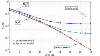
Figure 4: Channel estimation mean squared error, $\alpha=0.99$

In Fig. 4, we show the channel estimation error due to our proposed design for different values of $N_{\sf d}$ (equivalently, different values of pilot density), when there is no interference (IF) and when there is interference (IP). When $N_{\sf d}$ increases, the channel estimation mean squared error also increases as expected. For the interference-free scenario, the corresponding error curves converge to each other and decrease almost linearly as the SNR increases (both curves are plotted in the log scale). This means that the impact of the fast fading is diminished in the high SNR regime. When the interference is present, there is a performance floor for channel estimation error. The results in Fig. 4 also validate the theoretical results stated in Propositions 1, 3, and 4 about the channel estimation errors in the scenarios without and with interference.

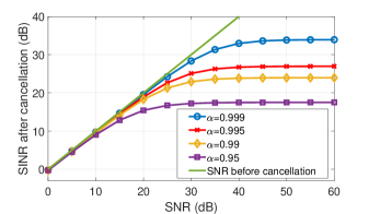
Figure 5: SINR after cancellation for different values of channel correlation coefficient, $N_{\sf d}=3$

In Fig. 5, we show the achieved SINR after interference cancellation versus the SNR for different values of channel correlation coefficient $\alpha$. Two noticeable observations can be drawn from this figure. First, it can be seen that the achieved SINR increases with increasing SNR before becoming saturated. In the low SNR regime, however, the residual interference has almost no impact on the achieved SINR after interference cancellation, i.e., the SINR curves after interference cancellation are very close to the line showing the SNR before interference cancellation. Second, the achieved SINR after cancellation increases with the increasing values of channel correlation coefficient $\alpha$. This is because the higher the value of $\alpha$ is, the lower the variance of the channel evolutionary noise and the less severe the impact of the fast fading are. Since the fast fading noise is less disruptive, interference cancellation performance is alleviated (as it is known that the fast fading noise causes the performance floor for the interference cancellation), which in turn reduces the residual interference power and makes the achieved SINR higher.

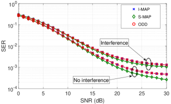
Figure 6: SER achieved by different detection methods, $N_{\sf d}=3$

V-C Performance of the Proposed Symbol Detection Methods

We now compare the SER performance of series symbol MAP detection (S-MAP), individual symbol MAP detection (I-MAP) and optimum diversity detection (ODD) [28, 30] methods. The ODD method is the optimum individual symbol detection with imperfect CSI. Basically, in the ODD method, the channel gains at data positions are interpolated from the MMSE-estimated channel gains at pilot positions. Then, the zero-forcing based symbol detection is employed (please refer to Sections III and IV in [30] for more details).

Fig. 6 illustrates the SER achieved by these detection methods for the interference-free and interference scenarios, which are denoted as IF and IP in this section, respectively. It can be seen that the SER of the proposed I-MAP is almost identical to that achieved by the ODD method. Moreover, the S-MAP detector outperforms both I-MAP and ODD and the performance gap is larger in the interference-free scenario. Note that, in the IP scenario, the residual interference still presents, which causes the error floors in these SER curves.

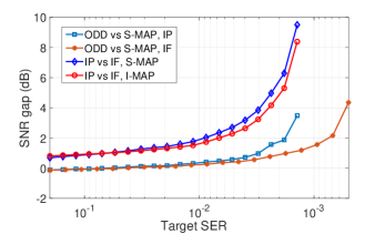
Figure 7: SNR gap for specific target SER, $N_{\sf d}=3$

For performance comparison between our methods and the existing method, we show in Fig. 7 the SNR gap to achieve the same SER between different symbol detection methods (S-MAP, I-MAP) and scenarios (IF, IP). Particularly, a value of 3dB SNR gap at $5\times 10^{-3}$ target SER of the curve A vs B means that method A needs 3dB higher in SNR to achieve the same target SER achieved by method B. For the same scenario (IF or IP), the SNR gap between the proposed S-MAP and ODD becomes larger as the required SER decreases. Note again that there is a performance floor in the IP scenario; nevertheless, our proposed detection method achieves more than 3dB SNR gain compared to the existing ODD method for the same detection performance in the low target SER regime (see the curve with square markers). Moreover, to achieve the same SER performance under the high reliability condition (i.e., low SER), the SNR required in the interference scenario is much higher than that required in the interference free scenario (illustrated by IP vs IF curves).

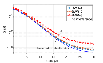
Figure 8: SER versus SNR for different values of BWR, $N_{\sf d}=3$

Fig. 8 illustrates the SER in the interference-free and interference scenarios for different bandwidth ratios, which is denoted as BWR. As can be seen from this figure, higher bandwidth ratios between interfering and desired signals lead to higher SER. This is because higher BWR creates more severe interference for the desired signal and it is not possible to completely remove the interference due to the fast fading.

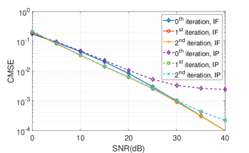
Figure 9: Performance of channel estimation for iterative algorithm

V-D Performance of the Iterative Algorithm

We now study the performance of the iterative algorithm for channel estimation, interference cancellation, and symbol detection. First, we present the performance of channel estimation over iterations in Fig. 9 where the CMSE of estimated channel gains is shown for both IF and IP scenarios. As can be seen from this figure, the iterative algorithm converges after only a few iterations. The most noticeable observation is that the converged channel estimation performance in the presence of interference (IP) is almost identical to that of the interference free scenario (IF) in the low SNR regime (less then 30dB), which implies that the proposed iterative method cancels very well the interference in this SNR region. When the SNR is higher than 30dB, the performance in the IP case is still limited by the fast fading noise. However, the performance floor of the iterative channel estimation approach is much lower than that of the non-iterative counterpart (the $0^{th}$-iteration versus the $2^{nd}$-iteration curves in the IP scenario).

We now study how the SER improves over iterations. In Fig. 10, the left and right figures show the SERs for the IF and IP cases, respectively. It can be seen from the figure that the SER improvement is higher when the interference is present, which suggests that the iterative algorithm estimates and cancels the interference effectively.

We show the SERs achieved by the non-iterative and iterative algorithms. From Fig. 11, we can see that the iterative algorithm improves the SER in both IF and IP scenarios. Furthermore, the improvement is higher for larger values of SNR. This is because that the high SNR regime allows more reliable data detection, which boosts the performance of interference cancellation and channel estimation.

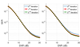
Figure 10: SER over iterations

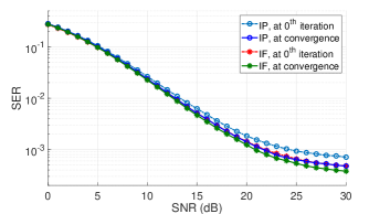
Figure 11: SER achieved by iterative and non-iterative algorithms

V-E Throughput Achieved by Proposed Framework

In Fig. 12, we show the variations of the throughput with the pilot density for different values of SNR $\rho$ and channel correlation coefficient $\alpha$. As can be seen from this figure, for given $\alpha$ and $\rho$, there exists an optimal pilot density that achieves the maximum throughput. Moreover, the maximum throughput increases as the SNR $\rho$ increases. It can also be observed that larger $\alpha$ leads to higher maximum throughput and lower optimal pilot density. This is because when the channel varies more slowly, the performance of interference cancellation and channel estimation is improved, which results in more reliable transmission and higher throughput. The results in this figure demonstrate the tradeoff between the throughput and communication reliability in the fast fading environment.

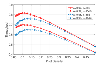
Figure 12: Throughput variations with the pilot density

VI Conclusion

We have proposed two frameworks for channel estimation, interference cancellation, and symbol detection for communication signals with different bandwidth in the fast fading environment. Specifically, in the two-phase non-iterative framework, we have derived the channel estimators and studied both series and individual symbol detection methods. The iterative framework performs interference cancellation, channel estimation and data detection based on the detected data symbol from the previous iteration, which can improve the system performance compared to the non-iterative counterpart. Numerical studies have confirmed the existence of the performance floor for SER in the considered interference scenario and illustrated the optimal pilot density to achieve the maximum throughput. Moreover, we have shown that the series symbol detection method outperforms the existing ODD method in terms of SER while the individual symbol detection method achieves the very close performance to the ODD method but with lower complexity.

Appendix A Proof of Theorem 1

To compute $p(\mathbf{h}_{n},\mathbf{Y})$, we need to find $p(\mathbf{Y}|\mathbf{h}_{n})$, since

$$p(\mathbf{h}_{n},\mathbf{Y})=p(\mathbf{Y}|\mathbf{h}_{n})p(\mathbf{h}_{n}),$$ (36)

and $p(\mathbf{h}_{n})$ is known to be $\mathcal{CN}(\mathbf{h}_{n},\mathbf{0},\mathbf{I}_{N_{\sf r}})$, where $\mathcal{CN}(\textbf{x},\boldsymbol{\mu},\boldsymbol{\Sigma})$ is the complex Gaussian density of random vector x having mean $\boldsymbol{\mu}$ and covariance matrix $\boldsymbol{\Sigma}$ [27]. The likelihood of $\mathbf{Y}$, given $\mathbf{h}_{n}$ can be factorized, thanks to the channel Markovian property, as

$$p(\mathbf{Y}|\mathbf{h}_{n}){=}p(\mathbf{y}_{n}|\mathbf{h}_{n})\!\prod_{i=1}^{n-1}{p(\mathbf{y}_{i}|\mathbf{y}_{i{+}1},\mathbf{h}_{n})}\!\!\!\prod_{i=n+1}^{N_{\sf p}}{\!\!p(\mathbf{y}_{i}|\mathbf{y}_{i{-}1},\mathbf{h}_{n})}.$$ (37)

Given $\mathbf{h}_{n}$, any two consecutive observations are correlated due to the cumulative channel evolutionary noises. Since we consider only received signals at pilot positions, the equivalent correlation coefficient of channel gains at two consecutive pilot positions is $\alpha_{\sf p}=\alpha^{N_{\sf d}+1}$. To further derive $p(\mathbf{Y}|\mathbf{h}_{n})$, we need to find the probabilities $p(\mathbf{y}_{i}|\mathbf{y}_{i-1},\mathbf{h}_{n})$ for $i>n$ and $p(\mathbf{y}_{i}|\mathbf{y}_{i+1},\mathbf{h}_{n})$ for $i<n$.

We now show the derivation of $p(\mathbf{y}_{i}|\mathbf{y}_{i-1},\mathbf{h}_{n})$ for $i>n$. From (8), the channel coefficient $\mathbf{h}_{i},i>n$ can be expressed with respect to $\mathbf{h}_{n}$ as

$$\mathbf{h}_{i}=\alpha_{\sf p}^{i-n}\left(\mathbf{h}_{n}+\eta_{\sf p}\sum_{j=1}^{i-n}{\alpha_{\sf p}^{-j}\boldsymbol{\Delta}_{n+j}}\right),\\$$ (38)

where $\eta_{\sf p}=\left(1{-}\alpha_{\sf p}^{2}\right)^{1/2}$. Substituting $\mathbf{h}_{n}$ in (38) into (9), it can be seen that $\mathbf{y}_{i}$ and $\mathbf{y}_{i-1}$ share the common evolutionary noise terms $\boldsymbol{\Delta}_{n+j},j=1,...,i{-}n{-}1$. Then, we can obtain the parameters of the distribution $p(\mathbf{y}_{i},\mathbf{y}_{i-1}|\mathbf{h}_{n})=$ $\mathcal{CN}\left(\!\left[\!\!\begin{array}[]{lll}\mathbf{y}_{i}\\ \mathbf{y}_{i-1}\end{array}\!\!\!\right]\!\!,\!\!\left[\!\!\begin{array}[]{lll}\boldsymbol{\mu}_{\mathbf{y}_{i}|\mathbf{h}_{n}}\\ \boldsymbol{\mu}_{\mathbf{y}_{i-1}|\mathbf{h}_{n}}\end{array}\!\!\right]\!\!,\!\!\left[\!\!\begin{array}[]{lll}\boldsymbol{\Sigma}_{\mathbf{y}_{i}|\mathbf{h}_{n}}\!\!&\!\!\!\boldsymbol{\Sigma}_{\mathbf{y}_{i},\mathbf{y}_{i-1}|\mathbf{h}_{n}}\\ \boldsymbol{\Sigma}_{\mathbf{y}_{i},\mathbf{y}_{i-1}|\mathbf{h}_{n}}^{H}\!\!&\!\!\!\boldsymbol{\Sigma}_{\mathbf{y}_{i-1}|\mathbf{h}_{n}}\end{array}\!\!\right]\right)$ as follows:

$$\begin{split}\boldsymbol{\mu}_{\mathbf{y}_{k}|\mathbf{h}_{n}}&{=}\mathbf{B}_{k}\mathbf{c}+\alpha_{\sf p}^{k-n}\mathbf{h}_{n}x_{k},\;k=i,i-1,\\ \boldsymbol{\Sigma}_{\mathbf{y}_{k}|\mathbf{h}_{n}}&{=}\left(\sigma^{2}{+}\alpha_{\sf p}^{2(k-n)}\eta_{\sf p}^{2}\sum_{j=1}^{k-n}{\alpha_{\sf p}^{-2j}}\right)\mathbf{I}_{N_{\sf r}}\\ &{=}\left[1{+}\rho\left(1-\alpha_{\sf p}^{2(k-n)}\right)\right]\sigma^{2}\mathbf{I}_{N_{\sf r}},\;k=i,i{-}1,\\ \boldsymbol{\Sigma}_{\mathbf{y}_{i},\mathbf{y}_{i{-}1}|\mathbf{h}_{n}}&{=}\operatorname{\mathbb{E}}\left[\left(\mathbf{y}_{i}{-}\boldsymbol{\mu}_{\mathbf{y}_{i}|\mathbf{h}_{n}}\right)\left(\mathbf{y}_{i-1}{-}\boldsymbol{\mu}_{\mathbf{y}_{i-1}|\mathbf{h}_{n}}\right)^{H}|\mathbf{h}_{n}\right]\\ &{=}x_{i}x_{i-1}^{*}\alpha_{\sf p}(1-\alpha_{\sf p}^{2(i-n-1)})\mathbf{I}_{N_{\sf r}}.\end{split}$$ (39)

Next, we apply the conditional probability formula for the multivariate Complex Circular Symmetric Gaussian vector [45] (section 3.7.7, page 153) and obtain $p(\mathbf{y}_{i}|\mathbf{y}_{i-1},\mathbf{h}_{n})=\mathcal{CN}(\mathbf{y}_{i},\boldsymbol{\mu}_{i,n},\boldsymbol{\Sigma}_{i,n})$ for $i>n$, where

$$\begin{split}\boldsymbol{\mu}_{i,n}&{=}\boldsymbol{\mu}_{\mathbf{y}_{i}|\mathbf{h}_{n}}+\beta_{i,n}\left(\mathbf{y}_{i-1}-\boldsymbol{\mu}_{\mathbf{y}_{i-1}|\mathbf{h}_{n}}\right),\\ \boldsymbol{\Sigma}_{i,n}&{=}\sigma_{i,n}^{2}\mathbf{I}_{N_{\sf r}},\;\beta_{i,n}=\frac{x_{i}x_{i-1}^{*}\rho\alpha_{\sf p}\left(1-\alpha^{2(i-n-1)}_{\sf p}\right)}{1+\rho\left(1-\alpha_{\sf p}^{2(i-n-1)}\right)},\\ \sigma_{i,n}^{2}&{=}\sigma^{2}\!\!\left[\!1{+}\rho\!\left(\!1{-}\alpha_{\sf p}^{2(i-n)}\!\right)\!{-}\frac{\rho^{2}\alpha^{2}_{\sf p}\left(1{-}\alpha_{\sf p}^{2(i-n-1)}\right)^{2}}{1{+}\rho\left(1{-}\alpha_{\sf p}^{2(i-n-1)}\right)}\right].\end{split}$$ (40)

For $i<n$, $p(\mathbf{y}_{i}|\mathbf{y}_{i+1},\mathbf{h}_{n})=\mathcal{CN}(\mathbf{y}_{i},\boldsymbol{\mu}_{i,n},\boldsymbol{\Sigma}_{i,n})$, where the parameters can be expressed similarly:

$$\boldsymbol{\mu}_{i,n}{=}\alpha^{n-i}_{\sf p}\mathbf{h}_{n}x_{i}{+}\mathbf{B}_{i}\mathbf{c}{+}\beta_{i,n}(\mathbf{y}_{i+1}{-}\alpha_{\sf p}^{n-i-1}\mathbf{h}_{n}x_{i+1}{-}\mathbf{B}_{i+1}\mathbf{c}),$$

$$\begin{split}\boldsymbol{\Sigma}_{i,n}&{=}\sigma_{i,n}^{2}\mathbf{I}_{N_{\sf r}},\;\;\beta_{i,n}=\frac{x_{i}x_{i+1}^{*}\rho\alpha_{\sf p}\left(1-\alpha^{2(n-i-1)}\right)}{1+\rho\left(1-\alpha_{\sf p}^{2(n-i-1)}\right)},\\ \sigma_{i,n}^{2}&{=}\sigma^{2}\!\!\left[\!1{+}\rho\!\left(\!1{-}\alpha_{\sf p}^{2(n-i)}\!\right)\!{-}\frac{\rho^{2}\alpha^{2}_{\sf p}\left(1{-}\alpha_{\sf p}^{2(n-i-1)}\right)^{2}}{1{+}\rho\left(1{-}\alpha_{\sf p}^{2(n-i-1)}\right)}\right].\end{split}$$ (41)

For $j=n,\boldsymbol{\mu}_{n,n}{=}\mathbf{h}_{n}x_{n}+\mathbf{B}_{n}\mathbf{c},\;\boldsymbol{\Sigma}_{n,n}{=}\sigma^{2}\mathbf{I}_{N_{\sf r}}$. Substituting the parameters in (40) and (41) into (36) using (37), taking the logarithm, we obtain the log-likelihood function in Theorem 1. This completes the proof.

Appendix B Proof for the Positive-definiteness of $\mathbf{D}_{n}$

For an arbitrary non-zero vector $\mathbf{z}=[z_{1},...,z_{L}]^{T}$, we have

$$\begin{split}\mathbf{z}^{H}\mathbf{D}_{n}\mathbf{z}&{=}\text{tr}\left[\left(\sum_{i=1}^{N_{\sf p}}{\frac{\left(\mathbf{B}_{i,n}\mathbf{z}\right)^{H}\left(\mathbf{B}_{i,n}\mathbf{z}\right)}{\sigma_{i,n}^{2}}}\right)\right]\\ -\text{tr}&\left[\left(\sum_{i=1}^{N_{\sf p}}{\frac{x^{*}_{i,n}\mathbf{B}_{i,n}}{\sigma_{i,n}^{2}}}\mathbf{z}\right)^{\!H}\!\!\mathbf{A}_{n}^{-1}\left(\sum_{i=1}^{N_{\sf p}}{\frac{x^{*}_{i,n}\mathbf{B}_{i,n}}{\sigma_{i,n}^{2}}}\mathbf{z}\right)\right]\\ &{=}\text{tr}\left[\left(\sum_{i=1}^{N_{\sf p}}{\frac{\left(\mathbf{B}_{i,n}\mathbf{z}\right)\left(\mathbf{B}_{i,n}\mathbf{z}\right)^{H}}{\sigma_{i,n}^{2}}}\right)\right]\\ -\text{tr}&\left[\left(\sum_{i=1}^{N_{\sf p}}{\frac{x^{*}_{i,n}\mathbf{B}_{i,n}}{\sigma_{i,n}^{2}}}\mathbf{z}\right)\mathbf{A}_{n}^{-1}\left(\sum_{i=1}^{N_{\sf p}}{\frac{x^{*}_{i,n}\mathbf{B}_{i,n}}{\sigma_{i,n}^{2}}}\mathbf{z}\right)^{\!H}\right]\\ &{>}\text{tr}\left[\left(\sum_{i=1}^{N_{\sf p}}{\frac{\left(\mathbf{B}_{i,n}\mathbf{z}\right)\left(\mathbf{B}_{i,n}\mathbf{z}\right)^{H}}{\sigma_{i,n}^{2}}}\right)\right.\\ -&\left.\!\!\left(\!\sum_{i=1}^{N_{\sf p}}{\frac{x^{*}_{i,n}\mathbf{B}_{i,n}}{\sigma_{i,n}^{2}}}\mathbf{z}\!\right)\!\!\left(\mathbf{A}_{n}{-}\mathbf{I}_{N_{\sf r}}\right)^{\!{-}1}\!\!\left(\!\sum_{i=1}^{N_{\sf p}}{\frac{x^{*}_{i,n}\mathbf{B}_{i,n}}{\sigma_{i,n}^{2}}}\mathbf{z}\!\!\right)^{\!\!\!\!H}\right]\!,\end{split}$$ (42)

where $\text{tr}(\mathbf{X})$ is the sum of diagonal elements of $\mathbf{X}$. In the last two lines of (42), the $j$th diagonal element of the first term is $\sum_{i=1}^{N_{\sf p}}{(\mathbf{b}_{i,n}^{(j)}\mathbf{z})(\mathbf{b}_{i,n}^{(j)}\mathbf{z})^{H}/\sigma_{i,n}^{2}}$, where $\mathbf{b}_{i,n}^{(j)}$ is the $j$th row of $\mathbf{B}_{i,n}$, and the $j$th diagonal element of the second term is $\left(\sum_{i=1}^{N_{\sf p}}{\frac{|x_{i,n}|^{2}}{\sigma_{i,n}^{2}}}\right)^{-1}\left(\sum_{i=1}^{N_{\sf p}}{\frac{x_{i,n}^{*}\mathbf{b}_{i,n}^{(j)}\mathbf{z}}{\sigma_{i,n}^{2}}}\right)\left(\sum_{i=1}^{N_{\sf p}}{\frac{x_{i,n}^{*}\mathbf{b}_{i,n}^{(j)}\mathbf{z}}{\sigma_{i,n}^{2}}}\right)^{H}$, where $\mathbf{A}_{n}$ from (14) is substituted into this term.

We now define the two vectors $\mathbf{u}$ and $\mathbf{v}$ whose $i$th elements are $\text{u}_{i}=x_{i,n}^{*}/\sigma_{i,n},\text{v}_{i}=\mathbf{b}_{i,n}^{(j)}\mathbf{z}/\sigma_{i,n}$, respectively. By applying the Cauchy-Schwarz inequality

$$|\mathbf{u}|^{2}|\mathbf{v}|^{2}\geq|\mathbf{u}.\mathbf{v}|^{2},$$ (43)

it can be verified that each diagonal element of the matrix in the last two lines of (42) is positive, which means its trace is also positive. Thus, we have completed the proof.

Appendix C Proof of Theorem 2

We can reformulate $p\left(x_{1:N_{\sf d}}|\mathbf{h}_{h},\mathbf{h}_{t},\mathbf{y}_{1:N_{\sf d}}\right)$ as follows:

$$\begin{split}&p\left(x_{1:N_{\sf d}}|\mathbf{h}_{h},\mathbf{h}_{t},\mathbf{y}_{1:N_{\sf d}}\right)\\ &{\propto}\int{p(x_{1:N_{\sf d}},\mathbf{y}_{1:N_{\sf d}},\mathbf{h}_{h},\mathbf{h}_{1:N_{\sf d}},\mathbf{h}_{t})d\mathbf{h}_{1:N_{\sf d}}}\\ &{\stackrel{{\scriptstyle(a)}}{{\propto}}}\int{p(\mathbf{y}_{1:N_{\sf d}}|\mathbf{h}_{1:N_{\sf d}},x_{1:N_{\sf d}})p(\mathbf{h}_{h},\mathbf{h}_{1:N_{\sf d}},\mathbf{h}_{t})d\mathbf{h}_{1:N_{\sf d}}}\\ &{\stackrel{{\scriptstyle(b)}}{{\propto}}}\int{p(\mathbf{h}_{h},\mathbf{h}_{1:N_{\sf d}},\mathbf{h}_{t})\prod_{i=1}^{N_{\sf d}}{p(\mathbf{y}_{i}|x_{i},\mathbf{h}_{i})}d\mathbf{h}_{1:N_{\sf d}}}\\ &{\stackrel{{\scriptstyle(c)}}{{\propto}}}\int{p(\mathbf{h}_{1}|\mathbf{h}_{h})p(\mathbf{h}_{t}|\mathbf{h}_{N_{\sf d}})\prod_{i=2}^{N_{\sf d}}{p(\mathbf{h}_{i}|\mathbf{h}_{i-1})}}\\ &\quad\quad\quad\quad\quad\quad\quad\quad\quad\quad\prod_{i=1}^{N_{\sf d}}{p(\mathbf{y}_{i}|x_{i},\mathbf{h}_{i})}d\mathbf{h}_{1:N_{\sf d}}\\ &{\stackrel{{\scriptstyle(d)}}{{\propto}}}\;e^{\mathcal{F}}\int{}{exp\left\{-\sum_{i=1}^{N_{\sf d}}{(\mathbf{h}_{i}-\mathbf{a}_{i})^{H}\mathbf{S}_{i}^{-1}(\mathbf{h}_{i}-\mathbf{a}_{i})}\right\}d\mathbf{h}_{1:N_{\sf d}}}\\ &{\stackrel{{\scriptstyle(e)}}{{\propto}}}\;e^{\mathcal{F}}\prod_{i=1}^{N_{\sf d}}{|\mathbf{S}_{i}|},\\ \end{split}$$ (44)

where $\boldsymbol{\Gamma}_{i,j}=\tau_{2}^{i-j}\prod_{k=j}^{i-1}{\mathbf{S}_{k}},\tau_{1}=\frac{1}{(1-\alpha^{2})\sigma^{2}_{\sf h}},\tau_{2}=\alpha\tau_{1},$ and $\mathcal{F}$ is defined in (24). Assuming all points in the constellation are transmitted with equal probability, the conditional probabilities in (44) are transformed by Baye’s rule $(a)$ and the Markovian property of channel $(b,c)$, where these expressions can be obtained by iteratively synthesizing quadratic terms of $\mathbf{h}_{i},i=1,...,N_{\sf d}$ in the exponents $(d,e)$.

Appendix D Proof of Proposition 1

The channel estimation error can be written as (see (14), (16))

$$\begin{split}\boldsymbol{\nu}_{n}&=\mathbf{h}_{n}-\mathbf{A}_{n}^{-1}\left(\sum_{i=1}^{N_{\sf p}}{\frac{x_{i,n}^{*}}{\sigma_{i,n}^{2}}}\left(\mathbf{y}_{i}-\beta_{i,n}\mathbf{y}_{i+j_{i,n}}\right)\right)\\ &=\boldsymbol{\nu}_{n}^{\sf g}+\boldsymbol{\nu}_{n}^{\sf c},\end{split}$$ (45)

where $\boldsymbol{\nu}_{n}^{\sf g}$ is the error due to the AWGN, and $\boldsymbol{\nu}_{n}^{\sf c}$ is the error due to the channel evolutionary noise. Specifically,

$$\begin{split}\boldsymbol{\nu}_{n}^{\sf g}&=\sum_{i=1}^{N_{\sf p}}{\boldsymbol{\Xi}_{i,n}^{\sf g}\mathbf{w}_{i}},\\ \boldsymbol{\nu}_{n}^{\sf c}&=\boldsymbol{\Xi}_{0,n}^{\sf c}\mathbf{h}_{0}+\sum_{i=1}^{N_{\sf p}}{\boldsymbol{\Xi}_{i,n}^{\sf c}\boldsymbol{\Delta}_{i}},\end{split}$$ (46)

where we decompose $\mathbf{h}_{n}$ into $\alpha_{\sf p}^{n}\left(\mathbf{h}_{0}+\sum_{i=1}^{n}{\alpha_{\sf p}^{-i}\boldsymbol{\Delta}_{i}}\right)$. By using this decomposition, it is more convenient to compute the channel estimation error components due to the channel evolutionary noise. Otherwise, one has to determine the dependence structure of $\mathbf{h}_{n}$ on the preceding channel noise components $\boldsymbol{\Delta}_{i},i<n$, which is not trivial.

When the desired channels are independent, $\boldsymbol{\Xi}_{i,n}^{\sf g}=\xi_{i,n}^{\sf g}\mathbf{I}_{N_{\sf r}}$ and $\boldsymbol{\Xi}_{i,n}^{\sf c}=\xi_{i,n}^{\sf c}\mathbf{I}_{N_{\sf r}}$. Substituting $\mathbf{y}_{i}=\mathbf{h}_{i}x_{i}+\mathbf{w}_{i}$ into (45), we have

$$\xi_{i,n}^{\sf g}{=}\left\{\begin{array}[]{ll}\!\!\!\!{-}\frac{x_{i,n}^{*}}{a_{n}\sigma_{i,n}^{2}},&\!\!\!\!i{=}1{,}n{,}n{\pm}1{,}N_{\sf p},\\ \!\!\!\!{-}\frac{x_{i}^{*}}{a_{n}}\left(\frac{\omega_{i,n}}{\sigma_{i,n}^{2}}{+}\frac{|\beta_{n,i-j_{i,n}}|\omega_{n,i-j_{i,n}}}{\sigma_{n,i-j_{i,n}}^{2}}\right)\!,&\!\!\!\!\text{otherwise}.\end{array}\right.$$

Hence, the AWGN contributes to the CEE with the total power of $\sigma^{2}\sum_{i=1}^{N_{\sf p}}{|\xi_{i,n}^{\sf g}|^{2}}$. As the SNR goes to infinity, $\text{lim}_{\rho\to\infty}\sum_{i=1}^{N_{\sf p}}{|\xi_{i,n}^{\sf g}|^{2}}=1$, and the AWGN contributes $\sigma^{2}$ to the overall CEE. Besides, $\boldsymbol{\nu}_{n}^{\sf c}$ is expressed in (48), and we can write the multipliers $\xi_{i,n}^{\sf c}$ as follows:

$$\begin{split}\xi_{0,n}^{\sf c}&=\alpha_{\sf p}^{n}-\sum_{i=1}^{N_{\sf p}}{\frac{\omega_{i,n}\alpha_{\sf p}^{i}}{a_{n}\sigma_{i,n}^{2}}(1-|\beta_{i,n}|\alpha_{\sf p}^{j_{i,n}})},\\ \xi_{i,n}^{\sf c}&=\frac{\alpha_{\sf p}^{-i}}{a_{n}}\left(\sum_{k=i-1}^{n-1}{\frac{\omega_{k,n}}{\sigma_{k,n}^{2}}|\beta_{k,n}|\alpha_{\sf p}^{k+1}}-\sum_{k=i}^{N_{\sf p}}{\frac{\omega_{k,n}}{\sigma_{k,n}^{2}}\alpha_{\sf p}^{k}}\right.\\ &\quad\quad\left.+\alpha_{\sf p}^{n}+\sum_{k=n+1}^{N_{\sf p}}{\frac{\omega_{k,n}}{\sigma_{k,n}^{2}}|\beta_{k,n}|\alpha_{\sf p}^{k-1}}\right),\;\;i\leq n,\\ \xi_{i,n}^{\sf c}&=\frac{\alpha_{\sf p}^{-i}}{a_{n}}\left(\sum_{k=i+1}^{N_{\sf p}}{\frac{\omega_{k,n}}{\sigma_{k,n}^{2}}|\beta_{k,n}|\alpha_{\sf p}^{k-1}}-\sum_{k=i}^{N_{\sf p}}{\frac{\omega_{k,n}}{\sigma_{k,n}^{2}}\alpha_{\sf p}^{k}}\right.\\ &\quad\left.-\frac{1}{\sigma^{2}}\mathds{1}_{n<N}\mathds{1}_{i=N}\right),\quad i>n.\end{split}$$ (47)

$$\begin{split}\boldsymbol{\nu}_{n}^{\sf c}&=\mathbf{h}_{n}-\mathbf{A}_{n}^{-1}\left\{\sum_{i=1}^{N_{\sf p}}{\frac{\omega_{i,n}\alpha_{\sf p}^{i}}{\sigma_{i,n}^{2}}\left[\mathbf{h}_{0}+\sum_{k=1}^{i}{\alpha_{\sf p}^{-k}\boldsymbol{\Delta}_{k}}-|\beta_{i,n}|\alpha_{\sf p}^{j_{i,n}}\left(\mathbf{h}_{0}+\sum_{k=1}^{i+j_{i,n}}{\alpha_{\sf p}^{-k}\boldsymbol{\Delta}_{k}}\right)\right]}\right\}\\ &=\mathbf{h}_{0}\left(\alpha_{\sf p}^{n}-\sum_{i=1}^{N_{\sf p}}{\frac{\omega_{i,n}\alpha_{\sf p}^{i}}{a_{n}\sigma_{i,n}^{2}}(1-|\beta_{i,n}|\alpha_{\sf p}^{j_{i,n}})}\right)-\sum_{k=1}^{N_{\sf p}}{\left(\boldsymbol{\Delta}_{k}\alpha_{\sf p}^{-k}\sum_{i=k}^{N_{\sf p}}{\frac{\omega_{i,n}}{a_{n}\sigma_{i,n}^{2}}\alpha_{\sf p}^{i}}\right)}+\sum_{i=1}^{n}{\alpha_{\sf p}^{n-i}\boldsymbol{\Delta}_{i}}\\ &+\sum_{k=1}^{n}{\left(\boldsymbol{\Delta}_{k}\alpha_{\sf p}^{-k}\sum_{i=k-1}^{n-1}{\frac{\omega_{i,n}}{a_{n}\sigma_{i,n}^{2}}|\beta_{i,n}|\alpha_{\sf p}^{i+1}}\right)}+\sum_{k=1}^{N_{\sf p}-1}{\left(\boldsymbol{\Delta}_{k}\alpha_{\sf p}^{-k}\sum_{i=k+1,i>n}^{N_{\sf p}}{\frac{\omega_{i,n}}{a_{n}\sigma_{i,n}^{2}}|\beta_{i,n}|\alpha_{\sf p}^{i-1}}\right)}\\ &=\mathbf{h}_{0}\left(\alpha_{\sf p}^{n}-\sum_{i=1}^{N_{\sf p}}{\frac{\omega_{i,n}\alpha_{\sf p}^{i}}{a_{n}\sigma_{i,n}^{2}}\left(1-|\beta_{i,n}|\alpha_{\sf p}^{j_{i,n}}\right)}\right)+\sum_{k=n+1}^{N-1}{\left[\boldsymbol{\Delta}_{k}\frac{\alpha_{\sf p}^{-k}}{a_{n}}\left(\sum_{i=k+1}^{N_{\sf p}}{\frac{\omega_{i,n}}{\sigma_{i,n}^{2}}|\beta_{i,n}|\alpha_{\sf p}^{i-1}}-\sum_{i=k}^{N_{\sf p}}{\frac{\omega_{i,n}}{\sigma_{i,n}^{2}}\alpha_{\sf p}^{i}}\right)\right]}\\ &{+}\sum_{k=1}^{n}{\!\left[\!\boldsymbol{\Delta}_{k}\frac{\alpha_{\sf p}^{-k}}{a_{n}}\!\!\left(\sum_{i=k{-}1}^{n-1}{\!\!\frac{\omega_{i,n}}{\sigma_{i,n}^{2}}|\beta_{i,n}|\alpha_{\sf p}^{i+1}}{-}\!\sum_{i=k}^{N_{\sf p}}{\frac{\omega_{i,n}}{\sigma_{i,n}^{2}}\alpha_{\sf p}^{i}}{+}\sum_{i=n+1}^{N_{\sf p}}{\frac{\omega_{i,n}}{\sigma_{i,n}^{2}}|\beta_{i,n}|\alpha_{\sf p}^{i-1}}\right)\right]}{+}\sum_{k=1}^{n}{\boldsymbol{\Delta}_{k}\alpha_{\sf p}^{n-k}}{-}\boldsymbol{\Delta}_{N}\frac{\omega_{N,n}}{a_{n}\sigma_{N,n}^{2}}\mathds{1}_{n<N}.\end{split}$$ (48)

As SNR goes to infinity, $\text{lim}_{\rho\to\infty}\sum_{i=1}^{N_{\sf p}}{|\xi_{i,n}^{\sf c}|^{2}}=0$, the channel evolutionary noises contribute negligible power to the CEE. This completes the proof.

Appendix E Proof of Proposition 2

Substituting $\mathbf{y}_{i,n}$ from (16) into (23), note that $\mathbf{y}_{i}=\mathbf{h}_{i}x_{i}+\mathbf{B}_{i}\mathbf{c}+\mathbf{w}_{i}$, and after some manipulations, we have

$$\begin{split}\tilde{\mathbf{c}}_{n}&=\mathbf{c}+\mathbf{D}_{n}^{-1}\sum_{i=1}^{N_{\sf p}}{\mathbf{G}_{i,n}\left(\mathbf{h}_{i}x_{i}+\mathbf{w}_{i}\right)},\end{split}$$ (49)

where $\mathbf{K}_{n}=\left(\sum_{i=1}^{N_{\sf p}}{x_{i,n}^{*}\boldsymbol{\Sigma}_{i,n}^{-1}\mathbf{B}_{i,n}}\right)^{H}\mathbf{A}_{n}^{-1},\mathbf{J}_{i,n}=\left(\mathbf{B}^{H}_{i,n}-\mathbf{K}_{n}x_{i,n}^{*}\right)\boldsymbol{\Sigma}_{i,n}^{-1}$, and

$$\mathbf{G}_{i,n}=\left\{\begin{array}[]{ll}\mathbf{J}_{i,n},&i{=}1,n,N_{\sf p}\\ \mathbf{J}_{i,n}-\mathbf{J}_{i-1,n}\beta_{i-1,n},&n>i>1\\ \mathbf{J}_{i,n}-\mathbf{J}_{i+1,n}\beta_{i+1,n},&n<i<N_{\sf p}.\end{array}\right.$$ (50)

The second term in (49) represents the estimation error of $\mathbf{c}$ at position $n$, and it is independent of $\mathbf{c}$. This completes the proof for the first part of the proposition.

Additionally, it can be seen that the estimation error is a linear combination of zero-mean Gaussian random variables, hence it also has zero mean. Therefore, the estimation is unbiased. The covariance matrix of the residual interference at position $n$th is

$$\begin{split}&(\sigma^{2}_{\sf h}{+}\sigma^{2})\operatorname{\mathbb{E}}_{(\mathbf{x},\mathbf{B})}\left[\mathbf{B}_{n}\mathbf{D}_{n}^{-1}\left(\sum_{i=1}^{N_{\sf p}}{\mathbf{G}_{i,n}\mathbf{G}_{i,n}^{H}}\right)\mathbf{D}_{n}^{-1}\mathbf{B}_{n}^{H}\right]\!\!{+}\\ &\sigma^{2}_{\sf h}\sum_{i\neq j}{\operatorname{\mathbb{E}}_{(\mathbf{x},\mathbf{B},\mathbf{h}_{i},\mathbf{h}_{j}\!)}\!\!\left[\!\mathbf{B}_{n}\mathbf{D}_{n}^{-1}\!\!\left(\!\mathbf{G}_{i,n}\mathbf{h}_{i}\mathbf{h}_{j}^{H}\mathbf{G}_{j,n}^{H}x_{i}x_{j}^{*}\!\right)\!\mathbf{D}_{n}^{-1}\mathbf{B}_{n}^{H}\right]}\\ &{=}(\sigma^{2}_{\sf h}{+}\sigma^{2})\operatorname{\mathbb{E}}_{(\mathbf{x},\mathbf{B})}\left[\mathbf{B}_{n}\mathbf{D}_{n}^{-1}\left(\sum_{i=1}^{N_{\sf p}}{\mathbf{G}_{i,n}\mathbf{G}_{i,n}^{H}}\right)\mathbf{D}_{n}^{-1}\mathbf{B}_{n}^{H}\right]\!\!{+}\\ &\;\sigma^{2}_{\sf h}\sum_{i\neq j}{\!\alpha_{\sf p}^{|i{-}j|}\operatorname{\mathbb{E}}_{(\mathbf{x},\mathbf{B})}\left[\mathbf{B}_{n}\mathbf{D}_{n}^{-1}\left(\mathbf{G}_{i,n}\mathbf{G}_{j,n}^{H}x_{i}x_{j}^{*}\right)\mathbf{D}_{n}^{-1}\mathbf{B}_{n}^{H}\right]}.\end{split}$$ (51)

Deriving the closed-form expression for the covariance matrix is tedious. Hence, we will prove Proposition 2 by using the following arguments. First, note that, $\mathbf{D}_{n}$ is Hermitian, positive definite, and in quadratic order of interfering matrices $\mathbf{B}_{i},i=1,...,N$. Second, $\mathbf{B}_{n}\mathbf{G}_{i,n}$ is also in quadratic order of interfering matrices. Therefore, the expected covariance matrix is in a fractional function form with total zero-th order of $\mathbf{B}_{i}$. As a result, the residual interference power is bounded as we increase the interference power to infinity. Furthermore, if all interfering channel coefficients for different antennas have identical value, the residual interference power is completely independent of the interference power. Since estimation errors for EICs at any symbol position $n$ are finite, the overall estimation error for EICs is also finite. This completes the proof.

Appendix F Proof of Proposition 3

Since the expression of the power of residual interference in (51) contains $\sigma^{2}_{\sf h}$, it does not vanish as $\rho\to\infty$. As $\rho$ goes to infinity, we have

$$\begin{split}\omega_{i,n}&{\to}\left\{\begin{array}[]{ll}\!\!\alpha_{\sf p},\!\!\!\!&i=n\pm 1\\ \!\!1,\!\!\!\!&i=n\\ \!\!0,\!\!\!\!&\text{otherwise}\\ \end{array}\right.\!\!\!,|\beta_{i,n}|\to\left\{\begin{array}[]{ll}\!\!0,\!\!\!\!&i=n,n\pm 1\\ \!\!\alpha_{\sf p},\!\!\!\!&\text{otherwise}\\ \end{array}\right.\!\!\!,\\ \sigma_{i,n}^{2}&{\to}\left\{\begin{array}[]{ll}\sigma^{2},&i=n\\ 1-a^{2}_{\sf p},&\text{otherwise}\end{array}\right.,\\ \mathbf{A}_{n}&{\to}\rho\mathbf{I}_{N_{\sf r}},\\ \mathbf{D}_{n}&{\to}\mathbf{B}_{n}^{H}\mathbf{B}_{n}+\sum_{i\neq n}^{N_{\sf p}}{\frac{\mathbf{B}_{i,n}^{H}\mathbf{B}_{i,n}}{1-\alpha_{\sf p}^{2}}}+2\frac{\alpha_{\sf p}^{2}}{1-\alpha_{\sf p}^{2}}\mathbf{B}_{n}^{H}\mathbf{B}_{n}\\ &\;-\frac{\alpha_{\sf p}}{1-\alpha_{\sf p}^{2}}\sum_{i=n\pm 1}{\left(x_{i}^{*}x_{n}\mathbf{B}^{H}_{n}\mathbf{B}_{i}+x_{i}x_{n}^{*}\mathbf{B}_{i}^{H}\mathbf{B}_{n}\right)}\\ &{\to}N_{\sf r}N_{\sf p}\frac{1+\alpha_{\sf p}^{2}}{1-\alpha_{\sf p}^{2}}\mathbf{I}_{L},\\ \mathbf{K}_{n}&\to x_{n}\mathbf{B}_{n}^{H},\\ \mathbf{J}_{n,n}&{\to}\mathbf{B}^{H}_{n}\frac{1+\alpha_{\sf p}^{2}}{1-\alpha_{\sf p}^{2}}-\frac{x_{n}^{*}\alpha_{\sf p}}{1-\alpha_{\sf p}^{2}}\sum_{i=n\pm 1}{x_{i}\mathbf{B}_{i}^{H}},\\ \mathbf{J}_{i,n}&{\to}\frac{\mathbf{B}_{i,n}^{H}-x_{n}x_{i}^{*}\alpha_{\sf p}\mathbf{B}_{n}^{H}}{1-\alpha_{\sf p}^{2}},i\neq n,\\ \mathbf{J}_{i,n}\mathbf{J}_{i,n}^{H}&{\to}N_{\sf r}\left(\frac{1+|\beta_{i,n}|^{2}+\omega_{i,n}^{2}}{\sigma_{i,n}^{4}}\right)\mathbf{I}_{L}\\ &{\to}\frac{N_{\sf r}\left(1+\alpha_{\sf p}^{2}\right)}{(1-\alpha_{\sf p}^{2})^{2}}\mathbf{I}_{L},i\neq n,\\ \mathbf{G}_{i,n}\mathbf{G}_{i,n}^{H}&{\to}\mathbf{J}_{i,n}\mathbf{J}_{i,n}^{H}{+}|\beta_{i\pm 1,n}|^{2}\mathbf{J}_{i\pm 1,n}\mathbf{J}_{i\pm 1,n}^{H}{+}\frac{2N_{\sf r}|\beta_{i\pm 1,n}|^{2}}{\sigma_{i,n}^{2}\sigma_{i\pm 1,n}^{2}}\mathbf{I}_{L}\\ &{\to}N_{\sf r}\frac{1+\alpha_{\sf p}^{4}+4\alpha_{\sf p}^{2}}{(1-\alpha_{\sf p}^{2})^{2}}\mathbf{I}_{L},i\neq n.\end{split}$$ (52)

Upon having these asymptotic values, we substitute these values into (51) to arrive at the residual interference power limit stated in the proposition, note that the computation of $\operatorname{\mathbb{E}}_{(\mathbf{x},\mathbf{B})}\left[\mathbf{B}_{n}\mathbf{D}_{n}^{-1}\left(\mathbf{G}_{i,n}\mathbf{G}_{j,n}^{H}x_{i}x_{j}^{*}\right)\mathbf{D}_{n}^{-1}\mathbf{B}_{n}^{H}\right],i\neq j,$ is done similarly. This completes the proof.

References

- [1] G. Naik, J. Liu, and J.-M. J. Park, “Coexistence of wireless technologies in the 5 GHz bands: a survey of existing solutions and a roadmap for future research,” IEEE Commun. Surveys Tuts., vol. 20, no. 3, pp. 1777–1798, Mar. 2018.
- [2] N. Lee and R. W. Heath Jr, “Advanced interference management technique: Potentials and limitations,” IEEE Wireless Commun., vol. 23, no. 3, pp. 30–38, June 2016.
- [3] Samsung Electronics Co. Ltd., “5G vision,” White paper, Aug. 2015.
- [4] Ericsson., “5G systems: Enabling the transportation of industry and society,” Available at https://www.ericsson.com/49daeb/assets/local/reports-papers/white-papers/wp-5g-systems.pdf (accessed on 2020/May/01), Jan. 2017.
- [5] S. A. A. Shah, E. Ahmed, M. Imran, and S. Zeadally, “5G for vehicular communications,” IEEE Commun. Mag., vol. 56, no. 1, pp. 111–117, Jan. 2018.
- [6] 3GPP, “Requirements for further advancements for evolved universal terrestrial radio access (E-UTRA) (LTE-Advanced),” Available at https://www.3gpp.org/DynaReport/36913.htm, July 2018.
- [7] J. Wu and P. Fan, “A survey on high mobility wireless communications: Challenges, opportunities and solutions,” IEEE Access, vol. 4, pp. 450–476, Apr. 2016.
- [8] G. Noh, J. Kim, H. Chung, and I. Kim, “Realizing Multi-Gbps vehicular communication: Design, implementation, and validation,” IEEE Access, vol. 7, pp. 19 435–19 446, Jan. 2019.
- [9] Y. Cai, Z. Qin, F. Cui, G. Y. Li, and J. A. McCann, “Modulation and multiple access for 5G networks,” IEEE Commun. Surveys Tuts., vol. 20, no. 1, pp. 629–646, 2017.
- [10] D. Bharadia, E. McMilin, and S. Katti, “Full duplex radios,” in Proc. ACM SIGCOMM Computer Commun. Rev., vol. 43, no. 4. ACM, 2013, pp. 375–386.
- [11] A. Sabharwal, P. Schniter, D. Guo, D. W. Bliss, S. Rangarajan, and R. Wichman, “In-band full-duplex wireless: Challenges and opportunities,” IEEE J. Sel. Areas Commun., vol. 32, no. 9, pp. 1637–1652, Sept. 2014.
- [12] E. Ahmed and A. M. Eltawil, “All-digital self-interference cancellation technique for full-duplex systems,” IEEE Trans. Wireless Commun., vol. 14, no. 7, pp. 3519–3532, July 2015.
- [13] D. Korpi, L. Anttila, V. Syrjälä, and M. Valkama, “Widely linear digital self-interference cancellation in direct-conversion full-duplex transceiver,” IEEE J. Sel. Areas Commun., vol. 32, no. 9, pp. 1674–1687, Sept. 2014.
- [14] M. T. Nguyen and L. B. Le, “Adjacent channel interference cancellation for robust spectrum sharing in satellite communications systems,” in Proc. IEEE PIMRC, 2017, pp. 1–5.
- [15] V. Syrjala, M. Valkama, L. Anttila, T. Riihonen, and D. Korpi, “Analysis of oscillator phase-noise effects on self-interference cancellation in full-duplex OFDM radio transceivers,” IEEE Trans. Wireless Commun., vol. 13, no. 6, pp. 2977–2990, June 2014.
- [16] E. Everett, A. Sahai, and A. Sabharwal, “Passive self-interference suppression for full-duplex infrastructure nodes,” IEEE Trans. Wireless Commun., vol. 13, no. 2, pp. 680–694, Feb. 2014.
- [17] M. Duarte, C. Dick, and A. Sabharwal, “Experiment-driven characterization of full-duplex wireless systems,” IEEE Trans. Wireless Commun., vol. 11, no. 12, pp. 4296–4307, Dec. 2012.
- [18] B. Debaillie, D.-J. van den Broek, C. Lavin, B. van Liempd, E. A. Klumperink, C. Palacios, J. Craninckx, B. Nauta, and A. Pärssinen, “Analog/RF solutions enabling compact full-duplex radios,” IEEE J. Sel. Areas Commun., vol. 32, no. 9, pp. 1662–1673, Sept. 2014.
- [19] K. Pedersen, G. Pocovi, J. Steiner, and A. Maeder, “Agile 5G scheduler for improved E2E performance and flexibility for different network implementations,” IEEE Commun. Mag., vol. 56, no. 3, pp. 210–217, Mar. 2018.
- [20] FCC, “Technical analysis of ligado interference impact on iridium user links,” Available at https://ecfsapi.fcc.gov/file/10902228186199/TechDescriptionofLigadoInterferenceImpact9.1.16-PUBLIC.pdf(accessed on 2020/May/01), Sep. 2016.
- [21] ERC, “Assessment of interference from unwanted emissions of NGSO MSS satellite transmitters operating in the space-to-earth direction in the band 1621.35 - 1626.5 MHz to GSO MSS satellite receivers operating in the earth-to-space direction in the band 1626.5 - 1660.5 MHz,” Available at https://www.ecodocdb.dk/download/148a1dcc-7c7a/REP091.PDF(accessed on 2020/May/01), Jun 2000.
- [22] K. Schwarzenbarth, J. Grotz, and B. Ottersten, “MMSE based interference processing for satellite broadcast reception,” in Proc. IEEE VTC Spring, 2007, pp. 1345–1349.
- [23] H. S. Wang and P.-C. Chang, “On verifying the first-order markovian assumption for a rayleigh fading channel model,” IEEE Trans. Veh. Technol., vol. 45, no. 2, pp. 353–357, May 1996.
- [24] G. E. Bottomley and S. Chennakeshu, “Unification of MLSE receivers and extension to time-varying channels,” IEEE Trans. Commun., vol. 46, no. 4, pp. 464–472, Apr. 1998.
- [25] C. C. Tan and N. C. Beaulieu, “On first-order markov modeling for the rayleigh fading channel,” IEEE Trans. Commun., vol. 48, no. 12, pp. 2032–2040, Dec. 2000.
- [26] S. Zhang, S.-C. Liew, and H. Wang, “Blind known interference cancellation,” IEEE J. Sel. Areas Commun., vol. 31, no. 8, pp. 1572–1582, Aug. 2013.
- [27] Y. Zhu, D. Guo, and M. L. Honig, “A message-passing approach for joint channel estimation, interference mitigation, and decoding,” IEEE Trans. Wireless Commun., vol. 8, no. 12, Dec. 2009.
- [28] N. Sun and J. Wu, “Maximizing spectral efficiency for high mobility systems with imperfect channel state information,” IEEE Trans. Wireless Commun., vol. 13, no. 3, pp. 1462–1470, Mar. 2014.
- [29] X. Ma, G. B. Giannakis, and S. Ohno, “Optimal training for block transmissions over doubly selective wireless fading channels,” IEEE Trans. Signal Process., vol. 51, no. 5, pp. 1351–1366, May 2003.
- [30] M. A. Mahamadu, J. Wu, Z. Ma, W. Zhou, Y. Tang, and P. Fan, “Fundamental tradeoff between doppler diversity and channel estimation errors in SIMO high mobility communication systems,” IEEE Access, vol. 6, pp. 21 867–21 878, Apr. 2018.
- [31] M. T. Nguyen and L. B. Le, “Channel estimation and symbol detection for communications on overlapping channels,” in Proc. IEEE Globecom Workshops (GC Wkshps), 2018, pp. 1–6.
- [32] H. Q. Ngo, H. A. Suraweera, M. Matthaiou, and E. G. Larsson, “Multipair full-duplex relaying with massive arrays and linear processing,” IEEE J. Sel. Areas Commun., vol. 32, no. 9, pp. 1721–1737, Sep. 2014.
- [33] X. Huang, K. Yang, F. Wu, and S. Leng, “Power control for full-duplex relay-enhanced cellular networks with QoS guarantees,” IEEE Access, vol. 5, pp. 4859–4869, Mar. 2017.
- [34] P. Sadeghi, R. A. Kennedy, P. B. Rapajic, and R. Shams, “Finite-state markov modeling of fading channels-a survey of principles and applications,” IEEE Signal Process. Mag., vol. 25, no. 5, pp. 57–80, Sep. 2008.
- [35] H. A. U. Mustafa, M. A. Imran, M. Z. Shakir, A. Imran, and R. Tafazolli, “Separation framework: An enabler for cooperative and D2D communication for future 5g networks,” IEEE Commun. Surveys Tuts., vol. 18, no. 1, pp. 419–445, 2016.
- [36] J. Hu, Y. Cai, and N. Yang, “Secure transmission design with feedback compression for the internet of things,” IEEE Trans. Signal Process., vol. 66, no. 6, pp. 1580–1593, Mar. 2018.
- [37] Q. Fenzhong and Y. Liuqing, “On the estimation of doubly-selective fading channels,” IEEE Trans. Wireless Commun., vol. 9, no. 4, pp. 1261–1265, Apr. 2010.
- [38] T. Zemen and A. F. Molisch, “Adaptive reduced-rank estimation of nonstationary time-variant channels using subspace selection,” IEEE Trans. Veh. Technol., vol. 61, no. 9, pp. 4042–4056, Sept. 2012.
- [39] C. Xu, J. Zhang, T. Bai, P. Botsinis, R. G. Maunder, R. Zhang, and L. Hanzo, “Adaptive Coherent/Non-Coherent Single/Multiple-Antenna aided channel coded ground-to-air aeronautical communication,” IEEE Trans. Commun., vol. 67, no. 2, pp. 1099–1116, Feb. 2019.
- [40] A. Yeredor, “The joint MAP-ML criterion and its relation to ml and to extended least-squares,” IEEE Trans. Signal Process., vol. 48, no. 12, pp. 3484–3492, Dec. 2000.
- [41] L. Tong, B. M. Sadler, and M. Dong, “Pilot-assisted wireless transmissions: general model, design criteria, and signal processing,” IEEE Signal Process. Mag., vol. 21, no. 6, pp. 12–25, June 2004.
- [42] A. T. Asyhari and S. ten Brink, “Orthogonal or superimposed pilots? a rate-efficient channel estimation strategy for stationary MIMO fading channels,” IEEE Trans. Wireless Commun., vol. 16, no. 5, pp. 2776–2789, May 2017.
- [43] Q. Shi, N. Wu, X. Ma, and H. Wang, “Frequency-domain joint channel estimation and decoding for faster-than-Nyquist signaling,” IEEE Trans. Commun., vol. 66, no. 2, pp. 781–795, Feb. 2018.
- [44] D. Tse and P. Viswanath, Fundamentals of wireless communication. Cambridge university press, 2005.
- [45] R. G. Gallager, Stochastic processes: theory for applications. Cambridge University Press, 2013.