Informative GANs via Structured
Regularization of Optimal Transport

Abstract

We tackle the challenge of disentangled representation learning in generative adversarial networks (GANs) from the perspective of regularized optimal transport (OT). Specifically, a smoothed OT loss gives rise to an implicit transportation plan between the latent space and the data space. Based on this theoretical observation, we exploit a structured regularization on the transportation plan to encourage a prescribed latent subspace to be informative. This yields the formulation of a novel informative OT-based GAN. By convex duality, we obtain the equivalent view that this leads to perturbed ground costs favoring sparsity in the informative latent dimensions. Practically, we devise a stable training algorithm for the proposed informative GAN. Our experiments support the hypothesis that such regularizations effectively yield the discovery of disentangled and interpretable latent representations. Our work showcases potential power of a regularized OT framework in the context of generative modeling through its access to the transport plan. Further challenges are addressed in this line.

1 Introduction

A central challenge in machine learning is that of disentangled representation learning [4] where the goal is to infer an interpretable and low-dimensional latent representation of the data. In this paper, we consider the setting of generative adversarial networks (GANs) [13] which aim to fit the data distribution $\nu$ as the transformation of some low-dimensional latent distribution $\zeta$ by a generator map $G$. Ideally, in a disentangled setting, variations of the latent code $z\sim\zeta$ should correspond to interpretable changes in the output $G(z)$.

Unlike existing works for disentangled and informative learning of GANs [6], our aim is to tackle this problem naturally within the framework of entropically smoothed optimal transport.

Optimal transport [28, 26, 22] and smoothed formulations thereof [8, 12, 9] have emerged as a promising and flexible framework for density fitting and generative modeling. In this vein, Sinkhorn losses were introduced in order to avoid biases due to the smoothing [12] and later put onto firm theoretical grounds [10, 9]. They were further applied to generative modeling and shown capable of delivering promising performance [25].

One interesting aspect of smoothed OT formulations we would like to focus on is the availability of the transportation plan via primal-dual optimality conditions. We will consider an implicit transportation plan which is given by a joint distribution over latent and visible variables. If this distribution were to coincide or be close to the true (unknown) joint distribution, it would certainly be useful for downstream tasks beyond generative modeling such as classification, uncertainty estimation or reinforcement learning.

As argued by the recent work [18], without inductive biases or regularizations there is no a priori reason why the learned transportation plan should be close to a “true” joint distribution with semantically meaningful latent variables. In this work, we encourage such inductive biases by adding an additional structured (concave) entropic regularization term to the formulation. The idea is to minimize the entropy of the transportation plan after marginalizing out an uninformative subset of the latent variables, thereby making the remaining variables more informative.

The other important aspect is the ground cost, which ideally is a semantically meaningful metric on the data space. To improve upon simple choices such as $\ell_{2}$-distances on pixel level, the works [12, 25, 17] learn the cost in an adversarial fashion. We show that a dual interpretation of our proposed structured regularization term connects to learned costs, but with a bias towards making transport on the informative dimensions cheaper. Due to simplicity, we will fix a simple $\ell_{1}$ or squared $\ell_{2}$ cost, which will be however be reasonable for the considered applications.

We organize the rest of the paper as follows:

• In Section 2.1 we review necessary background on (smoothed) optimal transport and generative modeling. Section 2.2 motivates the use of the Sinkhorn loss, confirming numerically that it helps alleviate variance collapse due to smoothing of the OT loss.

• In Section 3.1, we expose the implicit transportation plan arising from the smoothed OT loss. Under the principle of mutual information maximization, this leads us to an informative generative model via structured entropic regularization on this plan; see Section 3.2. By convex duality, we offer an interpretation as a (biased) learning of the ground cost. We further devise a practical training algorithm for deep generative models in Section 3.3.

• Our experiments on MNIST in Section 4 show that the proposed structured regularization indeed encourages disentangled latent representations. Section 5 concludes the paper with a discussion.

$\mathcal{W}_{c,\varepsilon}:c(x,y)=\|x-y\|_{1}$

(a)

$\mathcal{S}_{c,\varepsilon}:c(x,y)=\left\|x-y\right\|_{1}$.

(b)

$\mathcal{W}_{c,\varepsilon}:c(x,y)=\left\|x-y\right\|_{2}^{2}$.

(c)

$\mathcal{S}_{c,\varepsilon}:c(x,y)=\left\|x-y\right\|_{2}^{2}$.

(d)

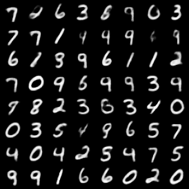
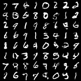
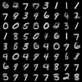
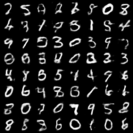
Figure 1: Comparison of smoothed OT loss $\mathcal{W}_{c,\varepsilon}$ and Sinkhorn loss $\mathcal{S}_{c,\varepsilon}$, all with $\varepsilon=0.001$. The entropic bias carried by the smoothed OT loss causes the generated samples to collapse on median (1(a)) and mean (1(c)) of clusters in the data. As shown in (1(b)) and (1(d)), the collapse is fixed by the debiasing term in the Sinkhorn loss.

2 Generative Modeling with the Sinkhorn Loss

In this section, we review optimal transport in the context of generative modeling, and then draw attention to the recently emerged Sinkhorn loss arising from optimal transport. For the rest of this paper, we adopt the measure-theoretic notations from [22].

2.1 Background on optimal transport and generative modeling

Let $c\in\mathcal{C}(\mathcal{X}\times\mathcal{X};\mathbb{R}_{+})$ be the ground cost over the compact metric space $\mathcal{X}$ such that $c(x,y)=0$ for all $x=y$. The optimal transport (OT) loss, traced back to Kantorovich [16], between two probability measures $\mu,\nu\in\mathcal{M}_{+}^{1}(\mathcal{X})$ is defined as

$$\mathcal{W}_{c}(\mu,\nu) =\inf_{\gamma\in\Gamma(\mu,\nu)}\int_{\mathcal{X}\times\mathcal{X}}c(x,y)\text{d}\gamma(x,y),$$ (1)

$$\Gamma(\mu,\nu) =\left\{\gamma\in\mathcal{M}_{+}^{1}(\mathcal{X}\times\mathcal{X}):\pi_{x\sharp}\gamma=\mu,\pi_{y\sharp}\gamma=\nu\right\}.$$ (2)

Given $G:\mathcal{Z}\to\mathcal{X}$ and $\zeta\in\mathcal{M}_{+}^{1}(\mathcal{Z})$, $G_{\sharp}\zeta$ denotes the pushforward measure [22, Definition 2.1]:

$$\forall h\in\mathcal{C}(\mathcal{X};\mathbb{R}):\int_{\mathcal{X}}h(x)dG_{\sharp}\zeta(x)=\int_{\mathcal{Z}}h(G(z))\text{d}\zeta(z).$$ (3)

With $\pi_{x}(x,y)=x$ and $\pi_{y}(x,y)=y$, the notations of pushforward measures $\pi_{x\sharp}\gamma$ and $\pi_{y\sharp}\gamma$ in (2) agree with the marginalization operations. The optimization variable $\gamma$ is referred to as the transportation plan.

In generative modeling, one aims to learn a generator $G\in\mathcal{C}(\mathcal{Z};\mathcal{X})$ that generates a realistic sample $x=G(z)$ from a latent code $z\sim\zeta$ under a fixed distribution $\zeta\in\mathcal{M}_{+}^{1}(\mathcal{Z})$. Equivalently speaking, one seeks for $G$ such that the pushforward measure $G_{\sharp}\zeta$ is as close as possible to a given empirical measure $\nu\in\mathcal{M}_{+}^{1}(\mathcal{X})$. Typically, the latent space $\mathcal{Z}$ is of much lower dimensions relative to the data space $\mathcal{X}$, yielding that both measures $G_{\sharp}\zeta$ and $\nu$ have singular supports. Legitimated by the fact that $\mathcal{W}_{c}$ metrizes the weak convergence of measures, e.g., if $c(x,y)=\|x-y\|_{p}^{p},~{}p\geq 1$ [28, Theorem 6.8], the OT loss $\mathcal{W}_{c}$ is well suited as the discrepancy measure between $G_{\sharp}\zeta$ and $\nu$. The generator learning can be stated as the minimum Kantorovich estimation [22, Section 9.4]:

$$\inf_{G\in\mathcal{C}(\mathcal{Z};\mathcal{X})}\mathcal{W}_{c}(G_{\sharp}\zeta,\nu) =\inf_{\begin{subarray}{c}G\in\mathcal{C}(\mathcal{Z};\mathcal{X})\\ \gamma\in\Gamma(G_{\sharp}\zeta,\nu)\end{subarray}}\int_{\mathcal{X}\times\mathcal{X}}c(x,y)\text{d}\gamma(x,y)$$ (4)

$$=\inf_{\begin{subarray}{c}G\in\mathcal{C}(\mathcal{Z};\mathcal{X})\\ \bar{\gamma}\in\Gamma(\zeta,\nu)\end{subarray}}\int_{\mathcal{Z}\times\mathcal{X}}c(G(z),y)\text{d}\bar{\gamma}(z,y).$$ (5)

The first identity above follows directly from the definition in (1). The second identity was shown in [5, Theorem 1], which justifies the equivalence of two formulations under the re-parameterization $\gamma=(G,\operatorname{id})_{\sharp}\bar{\gamma}$. This re-parameterization will be further exploited in Section 3.

In the literature, the seminal work on the Wasserstein GANs [1] approaches the training of (4) by introducing discriminator (networks) $D_{1},D_{2}$ into play, i.e.,

$$\inf_{G\in\mathcal{C}(\mathcal{Z};\mathcal{X})}\sup_{D_{1},D_{2}\in\mathcal{C}(\mathcal{X};\mathbb{R})}~{}\bigg{\{}\int_{\mathcal{Z}}D_{1}(G(z))\text{d}\zeta(z)+\int_{\mathcal{X}}D_{2}(y)\text{d}\nu(y)$$

$$\qquad\text{subject to}~{}D_{1}(x)+D_{2}(y)\leq c(x,y)\text{for }(x,y)~{}\text{($G_{\sharp}\zeta\otimes\nu$)-a.e.}\bigg{\}}.$$ (6)

The optimal pair $(D_{1},D_{2})$ complies with the $c$-transform relation [28, Definition 5.2]:

$$\!\!\forall x\in\mathcal{X}:D_{1}(x)=D_{2}^{(c)}(x):=\inf_{y\in\mathcal{X}}\big{\{}c(x,y)-D_{2}(y)\big{\}}.$$ (7)

Provided that $c$ is a metric, the $c$-transform in (7) specializes to $D_{1}=-D_{2}$ with an additional constraint of $D_{2}$ being 1-Lipschitz, cf. [28, Particular Case 5.4]. This leads to a minimax problem over a generator and a (single) discriminator [1], akin to the formulation of the original GAN [13]. The 1-Lipschitz constraint is numerically challenging and often pursued heuristically, e.g., by weight clipping [1], gradient penalty [14] or spectral normalization [19].

2.2 Minimum Sinkhorn estimation

More recently, the Sinkhorn loss has drawn interests as a smoothed variant for the OT loss; see [12, 9, 10]. With the Kullback-Leibler (KL) divergence defined by

$$\operatorname{KL}\left(\mu\,\middle|\,\nu\right)=\begin{cases}\int_{\mathcal{X}}\log\left(\frac{\text{d}\mu}{\text{d}\nu}(x)\right)\text{d}\mu(x)\!&\text{if $\frac{\text{d}\mu}{\text{d}\nu}$ exists $\nu$-a.e.}\\ \infty&\text{otherwise,}\end{cases}$$ (8)

the Sinkhorn loss $\mathcal{S}_{c,\varepsilon}$ is defined through the entropic regularized OT loss $\mathcal{W}_{c,\varepsilon}$:

$$\mathcal{S}_{c,\varepsilon}(\mu,\nu)=\mathcal{W}_{c,\varepsilon}(\mu,\nu)-\frac{1}{2}\mathcal{W}_{c,\varepsilon}(\mu,\mu)-\frac{1}{2}\mathcal{W}_{c,\varepsilon}(\nu,\nu),$$ (9)

$$\mathcal{W}_{c,\varepsilon}(\mu,\nu)=\inf_{\gamma\in\Gamma(\mu,\nu)}\bigg{\{}\int_{\mathcal{X}\times\mathcal{X}}c(x,y)\text{d}\gamma(x,y)+\varepsilon\cdot\operatorname{KL}\left(\gamma\,\middle|\,\mu\otimes\nu\right)\bigg{\}}.$$ (10)

In this work, we consider generative modeling via minimum Sinkhorn estimation:

$$\inf_{G\in\mathcal{C}(\mathcal{Z};\mathcal{X})}\mathcal{S}_{c,\varepsilon}(G_{\sharp}\zeta,\nu)=\inf_{G\in\mathcal{C}(\mathcal{Z};\mathcal{X})}\bigg{\{}\mathcal{W}_{c,\varepsilon}(G_{\sharp}\zeta,\nu)-\frac{1}{2}\mathcal{W}_{c,\varepsilon}(G_{\sharp}\zeta,G_{\sharp}\zeta)-\frac{1}{2}\mathcal{W}_{c,\varepsilon}(\nu,\nu)\bigg{\}}.$$ (11)

Promising empirical results on generative modeling in the spirit of (11) were obtained recently in [24, 25]. Note that the last term $-\frac{1}{2}\mathcal{W}_{c,\varepsilon}(\nu,\nu)$ is a constant which can be safely ignored in the training of $G$.

The advantages of using $\mathcal{S}_{c,\varepsilon}$ rather than $\mathcal{W}_{c}$ or $\mathcal{W}_{c,\varepsilon}$ as the training loss are previously observed in literature and summarized in the following:

• The regularization by KL divergence renders $\mathcal{W}_{c,\varepsilon}(\mu,\nu)$ (and hence $\mathcal{S}_{c,\varepsilon}(\mu,\nu)$ as well) Fréchet-differentiable with respect to $\mu$, see [9, Proposition 2]. The smoothness of the generative objective was exploited in [25].

• The Sinkhorn loss $\mathcal{S}_{c,\varepsilon}$ induces a divergence which interpolates between the OT distance $\mathcal{W}_{c}$ (letting $\varepsilon\to 0$) and the maximum mean discrepancy (MMD) [27] (letting $\varepsilon\to\infty$). In this respect, $\mathcal{S}_{c,\varepsilon}$ metrizes the weak convergence of measures same as $\mathcal{W}_{c}$ does [9, Theorem 1], while enjoying a better sample complexity than $\mathcal{W}_{c,\varepsilon}$ [12, 10].

• The entropic regularization in $\mathcal{W}_{c,\varepsilon}$ observably introduces bias [25, 9] since in general $\mathcal{W}_{c,\varepsilon}(\mu,\mu)\neq 0$. Remarkably, the inclusion of the debiasing term $-\frac{1}{2}\mathcal{W}_{c,\varepsilon}(G_{\sharp}\zeta,G_{\sharp}\zeta)$ in (11) accounts for avoiding a mode collapse of $G_{\sharp}\zeta$ towards a shrunk measure (e.g., median of $\nu$ if $c(x,y)=\|x-y\|_{1}$ or mean of $\nu$ if $c(x,y)=\|x-y\|_{2}^{2}$), see [9, Figure 1] on a 2D toy example and Figure 1 on MNIST.

(a) $\varepsilon=20$, $\lambda=0$

(b) $\varepsilon=20$, $\lambda=5$

Figure 2: We compute two transportation plans $\gamma^{\prime}$ and $\gamma$ with $c(x,y)=\left\|x-y\right\|^{2}$ and marginals $\zeta$ and $\nu$. $\zeta$ is uniform on the unit square, and $\nu$ is a mixture of 1D Gaussians supported only on a diagonal of the unit square. In (2(a)), the plan $\gamma^{\prime}$ is obtained without informative regularization, i.e., $\lambda=0$ in (19), and is therefore rather diffuse. For (2(b)), we switch on the informative regularization ($\lambda=5$) and observe that it makes the latent dimension $z_{1}$ informative, indicated by a sparse support of $\pi_{(z_{1},y)\sharp}\gamma$.

3 Informative Sinkhorn GANs

Learning disentangled representations is the holy grail of generative modeling, see the discussion in Section 1. Inspired by mutual information maximization in InfoGAN [6] and InfoVAE [29], we propose to include an additive regularization term in the minimum Sinkhorn estimation (11) such that a prescribed latent subspace is encouraged to be informative. The key to access this regularization is the implicit transportation plan arising from the smoothed OT loss $\mathcal{W}_{c,\varepsilon}(G_{\sharp}\zeta,\nu)$.

3.1 Implicit transportation plan

In the context of generative modeling, the Fenchel dual formulation of the smoothed OT loss $\mathcal{W}_{c,\varepsilon}(G_{\sharp}\zeta,\nu)$ (recall the definition from (10)) is given by

$$\mathcal{W}_{c,\varepsilon}(G_{\sharp}\zeta,\nu)=\inf_{\gamma\in\Gamma(G_{\sharp}\zeta,\nu)}\bigg{\{}\int_{\mathcal{X}\times\mathcal{X}}c(x,y)\text{d}\gamma(x,y)+\varepsilon\cdot\operatorname{KL}\left(\gamma\,\middle|\,G_{\sharp}\zeta\otimes\nu\right)\bigg{\}}$$ (12)

$$=\sup_{D_{1},D_{2}\in\mathcal{C}(\mathcal{X};\mathbb{R})}\bigg{\{}\int_{\mathcal{Z}}D_{1}(G(z))\text{d}\zeta(z)+\int_{\mathcal{X}}D_{2}(y)\text{d}\nu(y)$$

$$\qquad\qquad-\int_{\mathcal{Z}\times\mathcal{X}}\varepsilon\exp\Big{(}\frac{1}{\varepsilon}\big{(}D_{1}(G(z))+D_{2}(y)-c(G(z),y)\big{)}\Big{)}\text{d}\zeta\otimes\nu(z,y)\bigg{\}}.$$ (13)

The optimal pair $\gamma$ and $(D_{1},D_{2})$ satisfies the conditions:

$$\pi_{x\sharp}\gamma=G_{\sharp}\zeta,~{}~{}\pi_{y\sharp}\gamma=\nu,$$ (14)

$$\frac{\text{d}\gamma}{d(G_{\sharp}\zeta\otimes\nu)}(x,y)=\exp\Big{(}\frac{1}{\varepsilon}\big{(}D_{1}(x)+D_{2}(y)-c(x,y)\big{)}\Big{)}.$$ (15)

In particular, these conditions guarantee that it is viable to re-parameterize $\gamma=(G,\operatorname{id})_{\sharp}\bar{\gamma}$ as stated in Theorem 1.

Theorem 1.

It is equivalent to re-parameterize $\gamma=(G,\operatorname{id})_{\sharp}\bar{\gamma}$ for the infimum in (12), that is

$$\mathcal{W}_{c,\varepsilon}(G_{\sharp}\zeta,\nu)=\inf_{\bar{\gamma}\in\Gamma(\zeta,\nu)}\bigg{\{}\int_{\mathcal{Z}\times\mathcal{X}}c(G(z),y)\text{d}\bar{\gamma}(z,y)+\varepsilon\cdot\operatorname{KL}\left((G,\operatorname{id})_{\sharp}\bar{\gamma}\,\middle|\,G_{\sharp}\zeta\otimes\nu\right)\bigg{\}}.$$ (16)

Proof.

On the one hand, $\gamma=(G,\operatorname{id})_{\sharp}\bar{\gamma}$ for $\bar{\gamma}\in\Gamma(\zeta,\nu)$ ensures the feasibility that $\gamma\in\Gamma(G_{\sharp}\zeta,\nu)$, and this specialization of $\gamma$ yields an inequality of (16) in the direction “$\leq$”. On the other hand, the optimal $\gamma$ satisfying (15) takes the form $\gamma=(G,\operatorname{id})_{\sharp}\bar{\gamma}$ with

$$\frac{\text{d}\bar{\gamma}}{d(\zeta\otimes\nu)}(z,y)=\exp\Big{(}\frac{1}{\varepsilon}\big{(}D_{1}(G(z))+D_{2}(y)-c(G(z),y)\big{)}\Big{)},$$ (17)

and hence (16) indeed holds with an equality. ∎

This implicit transportation plan $\bar{\gamma}\in\mathcal{M}_{+}^{1}(\mathcal{Z}\times\mathcal{X})$ contains rich information as $\bar{\gamma}$ is a reasonable proxy for the joint distribution of the latent code and the generated image. We will further exploit this observation in the next subsection so as to make generator $G$ informative.

3.2 Informative minimum Sinkhorn estimation via structured regularization

We first introduce necessary notations. Let the latent space be decomposed as $\mathcal{Z}=\mathcal{Z}_{1}\times\mathcal{Z}_{2}$ with the intended informative subspace $\mathcal{Z}_{1}$ and its noisy counterpart $\mathcal{Z}_{2}$. Furthermore, let $\pi_{z_{1}}(z_{1},z_{2})=z_{1},~{}\pi_{(z_{1},y)}(z_{1},z_{2},y)=(z_{1},y)$ and $\zeta=\zeta_{1}\otimes\zeta_{2}$ with $\zeta_{1}\in\mathcal{M}_{+}^{1}(\mathcal{Z}_{1})$ and $\zeta_{2}\in\mathcal{M}_{+}^{1}(\mathcal{Z}_{2})$.

Given a latent code $z=(z_{1},z_{2})\sim\zeta$, $z_{1}$ being informative would yield high mutual information between $z_{1}$ and $x=G(z)$, which can be quantified through the KL divergence [7, Section 2.3]:

$$\operatorname{MI}((z_{1},x)\sim(\pi_{z_{1}},G)_{\sharp}\zeta)=\operatorname{KL}\left((\pi_{z_{1}},G)_{\sharp}\zeta\,\middle|\,\zeta_{1}\otimes G_{\sharp}\zeta\right).$$ (18)

Invoking the transportation plan $\bar{\gamma}$ in the formulation (16) as a proxy for $(\pi_{z_{1}},G)_{\sharp}\zeta$, we come up with the following informative minimum Sinkhorn estimation:

$$\inf_{\begin{subarray}{c}G\in\mathcal{C}(\mathcal{Z};\mathcal{X})\\ \bar{\gamma}\in\Gamma(\zeta,\nu)\end{subarray}}\bigg{\{}\int_{\mathcal{Z}\times\mathcal{X}}c(G(z),y)\text{d}\bar{\gamma}(z,y)+\varepsilon\cdot\operatorname{KL}\left((G,\operatorname{id})_{\sharp}\bar{\gamma}\,\middle|\,G_{\sharp}\zeta\otimes\nu\right)$$

$$\qquad\qquad\qquad-\frac{1}{2}\mathcal{W}_{c,\varepsilon}(G_{\sharp}\zeta,G_{\sharp}\zeta)-\lambda\cdot\operatorname{KL}\left(\pi_{(z_{1},y)\sharp}\bar{\gamma}\,\middle|\,\zeta_{1}\otimes\nu\right)\bigg{\}}.$$ (19)

The structured entropic regularization (the negative $\lambda\cdot$KL term) drives entropy of the marginalized transportation plan $\pi_{(z_{1},y)\sharp}\bar{\gamma}$ low and in return $z_{1}\sim\zeta_{1}$ to be informative. Figure 2 illustrates the effect of this regularization through a toy example. For that example we fix $G=\operatorname{id}$ and for the numerical solution, we adopt a DC strategy [15] and solve a sequence of perturbed problems with the Sinkhorn algorithm [8].

To gain further insights on our model (19), let us consider the dual formulation of the KL divergence used in [20, 21, 3]:

$$\operatorname{KL}\left(\pi_{(z_{1},y)\sharp}\bar{\gamma}\,\middle|\,\zeta_{1}\otimes\nu\right) =\sup_{Q\in\mathcal{C}(\mathcal{Z}_{1}\times\mathcal{X};\mathbb{R})}\bigg{\{}\int_{\mathcal{Z}\times\mathcal{X}}Q(z_{1},y)\text{d}\bar{\gamma}(z,y)+1$$

$$\qquad-\int_{\mathcal{Z}_{1}\times\mathcal{X}}\exp\big{(}Q(z_{1},y)\big{)}\text{d}\zeta_{1}\otimes\nu(z_{1},y)\bigg{\}}.$$ (20)

For a formal proof of the above equality, we refer the interested reader to [9, Proposition 7]. Using the dual formulation (20), we convert (19) into the form:

$$\inf_{\begin{subarray}{c}G\in\mathcal{C}(\mathcal{Z};\mathcal{X})\\ \bar{\gamma}\in\Gamma(\zeta,\nu)\\ Q\in\mathcal{C}(\mathcal{Z}_{1}\times\mathcal{X};\mathbb{R})\end{subarray}}\bigg{\{}\int_{\mathcal{Z}\times\mathcal{X}}\Big{(}c(G(z),y)-\lambda Q(z_{1},y)\Big{)}\text{d}\bar{\gamma}(z,y)+\varepsilon\cdot\operatorname{KL}\left((G,\operatorname{id})_{\sharp}\bar{\gamma}\,\middle|\,G_{\sharp}\zeta\otimes\nu\right)$$

$$\qquad\qquad\qquad-\frac{1}{2}\mathcal{W}_{c,\varepsilon}(G_{\sharp}\zeta,G_{\sharp}\zeta)\lambda+\lambda\int_{\mathcal{Z}_{1}\times\mathcal{X}}\exp\big{(}Q(z_{1},y)\big{)}\text{d}\zeta_{1}\otimes\nu(z_{1},y)\bigg{\}}.$$ (21)

That way, we can interpret the variational variable $Q$ in (21) in the language of optimal transport: $Q$ learns to modify the (pulled-back) ground cost $c\circ(G,\operatorname{id})$, with a bias towards making the marginalized transportation plan $\pi_{(z_{1},y)\sharp}\bar{\gamma}$ informative (i.e. low entropy).

Note that there are various ways to obtain variational lower bound to the mutual information, see [23] for a recent survey. Our bound (20) is based on convex duality, which we found to be natural within the framework of optimal transport. Another bound is the one of Barber and Agakov [2] given by

$$\operatorname{KL}\left(\pi_{(z_{1},y)\sharp}\bar{\gamma}\,\middle|\,\zeta_{1}\otimes\nu\right)\geq\int_{\mathcal{Z}\times\mathcal{X}}\log q(z_{1}|y)\,\text{d}\bar{\gamma}(z,y),$$ (22)

where $q(z_{1}|y)$ is the density, with respect to $\zeta_{1}$, of an arbitrary conditional distribution on $z_{1}$ given $y$. Note that (22) can be recovered from (20) by selecting the special parametrization $Q(z_{1},y)=\log q(z_{1}|y)$.

The main conceptual difference to InfoGAN [6], which maximizes the mutual information between the latent and generated variables (18) via the variational lower bound (22), is that we consider the transport plan $\bar{\gamma}$ as a proxy for the true, but intractable, joint distribution. Interestingly enough, it can be noted that our $Q$ only operates on real data samples, as opposed to the “$Q$ network” developed in [6]. In such a setting, our $Q$ influences the generator $G$ through modifying the (pulled back) ground cost.

3.3 A practical training algorithm

Here we derive a practical training scheme for model (19). Based on the formulation (21), we compute the associated OT loss via its dual formulation:

$$\inf_{\bar{\gamma}\in\Gamma(\zeta,\nu)}\bigg{\{}\int_{\mathcal{Z}\times\mathcal{X}}\Big{(}c(G(z),y)-\lambda Q(z_{1},y)\Big{)}\text{d}\bar{\gamma}(z,y)+\varepsilon\cdot\operatorname{KL}\left((G,\operatorname{id})_{\sharp}\bar{\gamma}\,\middle|\,G_{\sharp}\zeta\otimes\nu\right)\bigg{\}}$$

$$=\sup_{D_{1},D_{2}\in\mathcal{C}(\mathcal{X};\mathbb{R})}\bigg{\{}\int_{\mathcal{Z}}D_{1}(G(z))\text{d}\zeta(z)+\int_{\mathcal{X}}D_{2}(y)\text{d}\nu(y)+\varepsilon$$

$$\qquad\qquad-\varepsilon\int_{\mathcal{Z}\times\mathcal{X}}\exp\Big{(}\frac{1}{\varepsilon}\big{(}D_{1}(G(z))+D_{2}(y)+\lambda Q(z_{1},y)-c(G(z),y)\big{)}\Big{)}\text{d}\zeta\otimes\nu(z,y)\bigg{\}},$$ (23)

$$=\sup_{D_{2}\in\mathcal{C}(\mathcal{X};\mathbb{R})}\bigg{\{}\int_{\mathcal{Z}}D_{2}^{(c,\varepsilon)}(G(z))\text{d}\zeta(z)+\int_{\mathcal{X}}D_{2}(y)\text{d}\nu(y)+\varepsilon\bigg{\}},$$ (24)

where $D_{1}$ is substituted by the $(c,\varepsilon)$-transform [22, Section 5.3] of $D_{2}$:

$$D_{2}^{(c,\varepsilon)}(\cdot)=-\varepsilon\log\int_{\mathcal{X}}\exp\Big{(}\frac{1}{\varepsilon}\big{(}D_{2}(y)-c(\cdot,y)\big{)}\Big{)}\text{d}\nu(y).$$ (25)

Compared to the $c$-transform in (7), the $(c,\varepsilon)$-transform can be viewed as a soft pointwise minimum on $c(\cdot,y)-D_{2}(y)$ over $y$. The derivation for (23)–(24) follows from an application of the Fenchel-Rockafellar’s theorem and can be found in [11, Proposition 2.1].

In a similar way, the second OT loss $\mathcal{W}_{c,\varepsilon}(G_{\sharp}\zeta,G_{\sharp}\zeta)$ in (21) is computed as

$$\mathcal{W}_{c,\varepsilon}(G_{\sharp}\zeta,G_{\sharp}\zeta)$$

$$=\inf_{\bar{\eta}\in\Gamma(\zeta,\zeta)}\bigg{\{}\int_{\mathcal{Z}\times\mathcal{Z}}c(G(z^{\prime}),G(z^{\prime\prime}))\text{d}\bar{\eta}(z^{\prime},z^{\prime\prime})+\varepsilon\cdot\operatorname{KL}\left((G,G)_{\sharp}\bar{\eta}\,\middle|\,G_{\sharp}\zeta\otimes G_{\sharp}\zeta\right)\bigg{\}}$$ (26)

$$=\sup_{D_{4}\in\mathcal{C}(\mathcal{X};\mathbb{R})}\bigg{\{}\int_{\mathcal{Z}}D_{4}^{(c,\varepsilon)}(G(z^{\prime}))\text{d}\zeta(z^{\prime})+\int_{\mathcal{Z}}D_{4}(G(z^{\prime\prime}))\text{d}\zeta(z^{\prime\prime})+\varepsilon\bigg{\}}.$$ (27)

Once again, a dual variable $D_{3}$ has been eliminated via the $(c,\varepsilon)$-transform:

$$D_{3}(\cdot)=D_{4}^{(c,\varepsilon)}(\cdot)$$

$$=-\varepsilon\log\int_{\mathcal{Z}}\exp\Big{(}\frac{1}{\varepsilon}\big{(}D_{4}(G(z^{\prime\prime}))-c(\cdot,G(z^{\prime\prime}))\big{)}\Big{)}\text{d}\zeta(z^{\prime\prime}).$$ (28)

With optimal dual variables $D_{2}$ and $D_{4}$ in hand, the optimal primal variables $\bar{\gamma}$ and $\bar{\eta}$ can be retrieved from the optimality conditions:

$$\frac{\text{d}\bar{\gamma}}{d(\zeta\otimes\nu)}(z,y)=\, \exp\Big{(}\frac{1}{\varepsilon}\big{(}D_{2}^{(c,\varepsilon)}(G(z))+D_{2}(y)+\lambda Q(z_{1},y)-c(G(z),y)\big{)}\Big{)},$$ (29)

$$\frac{\text{d}\bar{\eta}}{d(\zeta\otimes\zeta)}(z^{\prime},z^{\prime\prime})=\, \exp\Big{(}\frac{1}{\varepsilon}\big{(}D_{4}^{(c,\varepsilon)}(G(z^{\prime}))+D_{4}(G(z^{\prime\prime}))-c(G(z^{\prime}),G(z^{\prime\prime}))\big{)}\Big{)}.$$ (30)

Our training algorithm alternates between $(\bar{\gamma},\bar{\eta})$ and $(Q,G)$. Specifically, we use the supremum problem (24) over $D_{2}$ (resp. (27) over $D_{4}$) and relation (29) (resp. (30)) as an oracle to update the expression for $\bar{\gamma}$ (resp. $\bar{\eta}$). Alternatively, given $\bar{\gamma}$ and $\bar{\eta}$ the variables $Q$ and $G$ can be updated in parallel through the following optimization:

$$\inf_{Q\in\mathcal{C}(\mathcal{Z}_{1}\times\mathcal{X};\mathbb{R})}\int_{\mathcal{Z}\times\mathcal{X}}-Q(z_{1},y)\text{d}\bar{\gamma}(z,y)+\int_{\mathcal{Z}_{1}\times\mathcal{X}}\exp\big{(}Q(z_{1},y)\big{)}\text{d}\zeta_{1}\otimes\nu(z_{1},y),$$ (31)

$$\inf_{G\in\mathcal{C}(\mathcal{Z};\mathcal{X})}\int_{\mathcal{Z}\times\mathcal{X}}c(G(z),y)\text{d}\bar{\gamma}(z,y)-\frac{1}{2}\int_{\mathcal{Z}\times\mathcal{Z}}c(G(z^{\prime}),G(z^{\prime\prime}))\text{d}\bar{\eta}(z^{\prime},z^{\prime\prime}).$$ (32)

The overall algorithm is spelled out in Algorithm 1.

Algorithm 1 Training scheme for model (19).

0:  $\zeta\in\mathcal{M}_{+}^{1}(\mathcal{Z}),~{}\nu\in\mathcal{M}_{+}^{1}(\mathcal{X}),~{}c\in\mathcal{C}(\mathcal{X}\times\mathcal{X};\mathbb{R}_{+}),~{}\varepsilon,\lambda>0,~{}n_{D}\in\mathbb{N}$.

1:  Initialize $D_{2},D_{4}\in\mathcal{C}(\mathcal{X};\mathbb{R}),\,G\in\mathcal{C}(\mathcal{Z};\mathcal{X}),\,Q\in\mathcal{C}(\mathcal{Z}_{1}\times\mathcal{X};\mathbb{R})$ as neural networks.

2:  while $G$ not converged do

3:     for $t=1,...,n_{D}$ do

4:        Draw minibatch samples $(z,y)\sim\zeta\otimes\nu$.

5:        Update the weights of $D_{2}$ by an Adam step on (24).

6:        Draw minibatch samples $(z^{\prime},z^{\prime\prime})\sim\zeta\otimes\zeta$.

7:        Update the weights of $D_{4}$ by an Adam step on (27).

8:     end for

9:     Express $\bar{\gamma}\in\mathcal{M}_{+}^{1}(\mathcal{Z}\times\mathcal{X})$ using (29) and $\bar{\eta}\in\mathcal{M}_{+}^{1}(\mathcal{Z}\times\mathcal{Z})$ using (30).

10:     Draw minibatch samples $(z,y,z^{\prime},z^{\prime\prime})\sim\zeta\otimes\nu\otimes\zeta\otimes\zeta$.

11:     Update in parallel the weights of $Q$ by an Adam step on (31) and the weights of $G$ by an Adam step on (32).

12:  end while

(a) Sinkhorn

(b) Info-Sinkhorn

(c) Sinkhorn

(d) Info-Sinkhorn

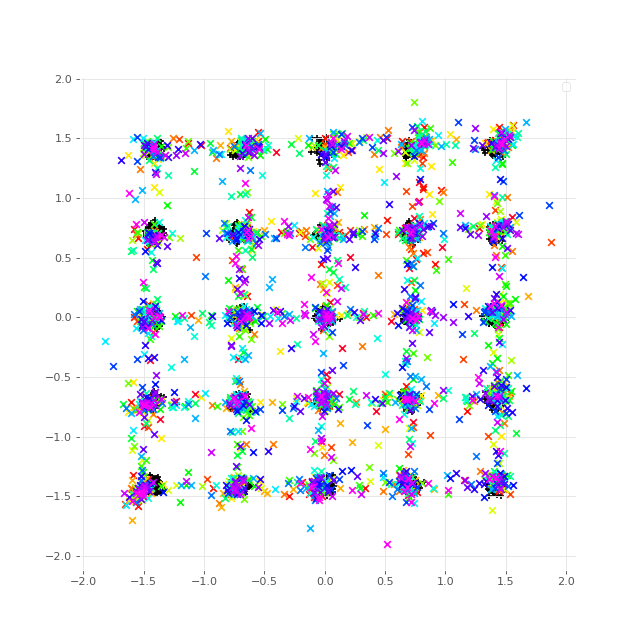
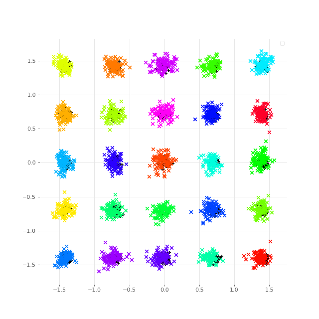
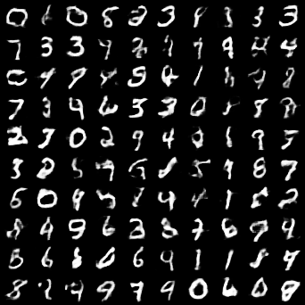
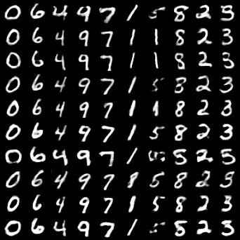
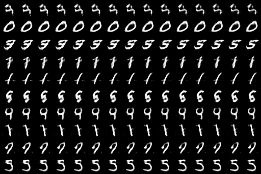
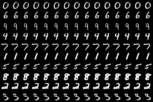
Figure 3: Variation of the categorical latent code on Gaussian dataset and MNIST, using $c(x,y)=\|x-y\|_{1}$, $\varepsilon=\lambda=0.05$. The categorical code is color-coded for the Gaussian dataset. From MNIST, each line has its categorical encoding varied while its other latent dimensions are kept constant. The continuous informative codes are set to zero, and for each row, the noisy dimensions are drawn according to $\zeta_{2}$. This categorical encoding is clear only for the informative models (3(d)).

4 Experiments

In this section, we demonstrate and discuss experimental results for the Info-Sinkhorn model trained by Algorithm 1. Our results are compared qualitatively to the baseline Sinkhorn model over two datasets: 2D multimodal Gaussians and MNIST.

4.1 Experimental setup

Regularization parameters.

Two main hyper-parameters are critical in the algorithm: $\varepsilon$ and $\lambda$. A good balanced choice is to have $\lambda$ equal to or slightly less than $\varepsilon$. Typically, we set $\lambda=\varepsilon\approx 0.05$. The complete training details can be found in Appendix A.

Network architectures.

The network architectures are adapted from previous works [6, 25, 14].

In particular, the discriminators $D_{\{2,4\}},D_{Q}$ are set to share their first (convolutional) layers and only learn the last layers independently. $D_{Q}$ shares its first layers with the discriminators $D_{\{2,4\}}$ as in [6].

The update of the shared parameters is only performed during the update of the dual networks $D_{\{2,4\}}$. Extensive sharing of layers and weights among the networks $D_{\{2,4\}}$ and $D_{Q}$ yields minimal computational overhead of the proposed informative generative model compared to existing GANs [13, 1, 6].

Parametrization of $Q$.

The Info-Sinkhorn model offers the liberty to parametrize the function $Q$ that appears in (21). In practice, we take a simple choice of a dot product rule, namely $Q(z_{1},x):=z_{1}^{\top}D_{Q}(x)$ where a network $D_{Q}$ outputs a vector of the same size as $z_{1}$. This parametrization, though being linear in $z_{1}$, already yields good disentanglement results on MNIST (see Section 4.3), and empirically works better than the $\log$-parametrization from (22) aligned with the InfoGAN [6].

(a) Sinkhorn, $z_{2}$

(b) Sinkhorn, $z_{3}$

(c) Sinkhorn, $z_{4}$

(d) Info-Sinkhorn, $z_{2}$

(e) Info-Sinkhorn, $z_{3}$

(f) Info-Sinkhorn, $z_{4}$

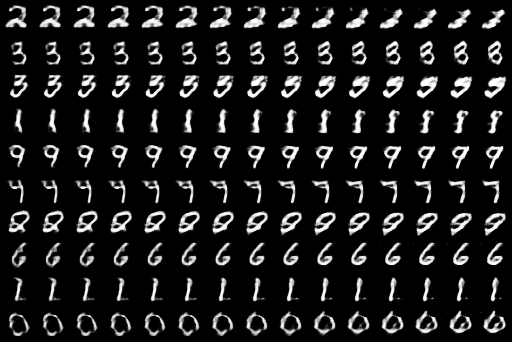
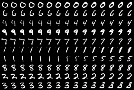
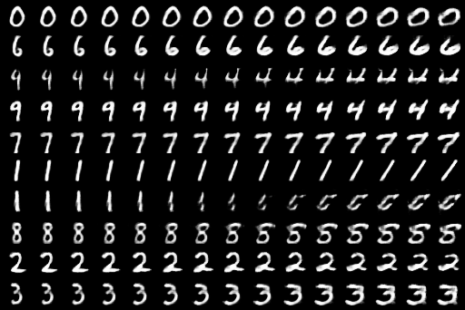
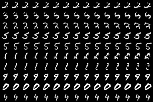
Figure 4: Variations in the latent space on the continuous code for MNIST. Upper row: Sinkhorn. Lower row: Info-Sinkhorn. $\varepsilon=\lambda=0.05$. Left two columns: two continuous informative latent variables $z_{2},z_{3}$. Right column: first noisy latent variable $z_{4}$. In each picture, each line represents a draw in the sample space, with a different categorical code, and which is fixed across all columns except for the appropriate continuous code $z_{i}$, which varies between $-1$ and $1$. There is a significant and interpretable visual variation only for the informative dimensions in the Info-Sinkhorn model (4(d)),(4(e)).

4.2 2D multimodal Gaussian dataset

A toy dataset is considered for testing the informative model, as it illustrates the learning algorithm quite well. A 25-modal 2D Gaussian dataset is learned, with a latent space factored into a 25-dimensional categorical (informative) part, and a 103 dimensional Gaussian (noisy) part. As can been seen in Fig. 3(a), the different modes are perfectly recovered, and even less artefacts are observed (as opposed to the baseline Sinkhorn model).

Although structurally simple, this dataset can be proven difficult to learn for standard GANs as mentioned in [25]. This illustrates the effectiveness of OT-based generative models when the underlying Euclidean space metric makes sense for comparing the samples: here the cost between samples $c(x,y)=\|x-y\|$ is natural. This strongly suggests that the proposed informative regularization on the transport plan can be relevant.

4.3 Latent space traversal on MNIST

We further test Info-Sinkhorn on MNIST. The latent factorization in this case is taken as follows: $z_{1}$ is an informative categorical code of dimension $10$, $z_{2},z_{3}\sim\text{Unif}[-1,1]$ are informative continuous latent codes. The remaining latent space $(z_{j})_{j=4}^{91}\sim\mathcal{N}(0,1)$ is designated to be the uninformative dimension.

In the different visualizations, each row represent a latent space traversal, and therefore has only one latent code that varies along the columns, whereas the other dimensions remain identical. This allows to visually evaluate the disentanglement and interpretability of the latent representation.

In Fig. 3(d), the ten categories in MNIST are well learned with the Info-Sinkhorn model. In contrast, for the baseline Sinkhorn model shown in Fig. 3(c) the categorical latent code has no clear interpretation. Moreover, given a row, the digit aspect remains similar across each columns. This shows how the style of a sample is mostly determined by the continuous latent space.

This is presented in more detail in Fig. 4. The informative model is compared to the Sinkhorn one, as to illustrate the effect of the proposed regularization on the output of the network. Although the visual cues are not perfectly disentangled (e.g. the rotation of certain digits is a result of both variations), the contrast is clear with the original Sinkhorn model, where the latent space configuration has unpredictable effects on the visual samples. The informative regularization yields on the contrary a much more disentangled and informative latent space.

5 Conclusion

This work advocates informative generative modeling via optimal transport. The entropic smoothing on an optimal transport loss enables access to the transportation plan. In the context of generative modeling, we introduce a novel structured regularization on this plan to make the prescribed latent dimensions informative. In this sense, our work bridges a gap between previous informative GANs [6] and smoothed optimal transport [22].

Practically, we derive an efficient training scheme for the proposed informative generative model, which is further boosted by extensive sharing of architectures and weights among multiple “discriminator” networks. We experimentally confirm that the recently introduced Sinkhorn loss [12, 9] indeed avoids collapses and that our proposed regularization yields informative latent representation and improved sample quality.

Although limited to a simple dataset, those experiments are a good sign of possible extensions for optimal transport GANs based on a structured transport plan regularization. The results in an Euclidean space where the ground cost was natural to compare samples suggests the offered method has potentials.

The generalization to more complex datasets is subject to defining/learning a better ground cost function $c(x,y)$, as optimal transport relies exhaustively on the metric of the underlying Euclidean space. For complex images, the pixel-wise metrics are not particularly adequate, and tend to produce blurred samples with very low variability. One dominant axis of research should be dedicated to finding a stable way to learn the cost jointly with the informative regularization.

Appendix A Training details

In the reported experiments, the Info-Sinkhorn model was trained using the following hyper-parameters. The baseline Sinkhorn model was trained with the exact same set of parameters, except for $\lambda=0$.

A.1 Gaussians

ground cost	$c(x,y)=\|x-y\|_{1}$
$d_{\text{cat}}$	25
$d_{\text{uni}}$	0
$d_{\text{noise}}$	103
$\varepsilon$	1.5
$\lambda$	1.0
$n_{D}$	5
Learning rate for $D_{i}$	0.0002
Learning rate for $G$	0.0002
Number of generator iter.	50000
Adam parameters	$\beta_{1}=0,\,\beta_{2}=0.9$

Table 1: Hyper-parameters for the Gaussian dataset

A.2 MNIST

ground cost	$c(x,y)=\|x-y\|_{1}$
$d_{\text{cat}}$	10
$d_{\text{uni}}$	2
$d_{\text{noise}}$	88
$\varepsilon$	0.05
$\lambda$	0.05
$n_{D}$	5
Weight decay on $Q$	0.001
Learning rate for $D_{i},Q$	0.0002
Learning rate for $G$	0.0002
Number of generator iter.	24200
Adam parameters	$\beta_{1}=0.5,\,\beta_{2}=0.99$

Table 2: Hyper-parameters for the MNIST dataset

Networks $D_{\{2,4\}},\,D_{Q}$
shared	Input 2D point
	FC 512 – b.n. – LReLU
	FC 512 – b.n. – LReLU
spec	FC 512 – b.n. – LReLU – $\big{[}\begin{array}[]{c}\text{FC 1 for}D_{\{2,4\}}\\ \text{FC }|\mathcal{Z}_{1}|\text{ for }D_{Q}\end{array}\big{.}$
Generator $G$
Input $z\in\mathcal{Z}\subset\mathbb{R}^{128}$
FC 512 – LReLU
FC 512 – LReLU
FC 512 – LReLU – FC 2

(a) Architecture for generating 2D multi-modal Gaussian data; adapted from [14].

Networks $D_{\{2,4\}},\,D_{Q}$
shared	Input 32x32x1 Gray image pixels
	4 x 4 conv. 64 (stride 2) – b.n. – LReLU
	4 x 4 conv. 128 (stride 2) – b.n. – LReLU
	FC 1024 – b.n. – LReLU
spec	– $\big{[}\begin{array}[]{c}\text{FC 1 for }D_{\{2,4\}}\\ \text{FC 128 -- b.n. -- LReLU -- FC }|\mathcal{Z}_{1}|\text{ for }D_{Q}\end{array}\big{.}$
Generator $G$
Input $z\in\mathcal{Z}\subset\mathbb{R}^{100}$
FC 1024 – b.n. – LReLU
FC $8\cdot 8\cdot 128$ – b.n. – LReLU
4 x 4 transp. conv. 64 (stride 2) – b.n. – LReLU
4 x 4 transp. conv. 1 (stride 2) – tanh

(b) Architecture for generating MNIST; adapted from [6].

Table 3: Architectures for the two datasets. Output dimension for fully connected layers (FC) is indicated. The kernel sizes and strides for 2D convolution (conv.) and transpose convolution (transp. conv.) are indicated, the input and output shapes being given by spatial convolution artihmetics. LeakyReLU (LReLU) activation functions with negative slope of $0.2$ are used in both generator and dual networks. Batchnorm (b.n.) is used when indicated.

References

• [1] M.ย Arjovsky, S.ย Chintala, and L.ย Bottou. Wasserstein generative adversarial networks. In International Conference on Machine Learning (ICML), 2017.
• [2] D.ย Barber and F.ย Agakov. The IM algorithm: a variational approach to information maximization. In Advances in Neural Information Processing Systems (NIPS), 2003.
• [3] M.ย I. Belghazi, A.ย Baratin, S.ย Rajeswar, S.ย Ozair, Y.ย Bengio, A.ย Courville, and Rย D. Hjelm. MINE: mutual information neural estimation. In International Conference on Machine Learning (ICML), 2018.
• [4] Y.ย Bengio, A.ย Courville, and P.ย Vincent. Representation learning: A review and new perspectives. Transactions on Pattern Analysis and Machine Intelligence (TPAMI), 35(8):1798โ€“1828, 2013.
• [5] O.ย Bousquet, S.ย Gelly, I.ย Tolstikhin, C.-J. Simon-Gabriel, and B.ย Schรถlkopf. From optimal transport to generative modeling: the VEGAN cookbook. arXiv:1705.07642, 2017.
• [6] X.ย Chen, Y.ย Duan, R.ย Houthooft, J.ย Schulman, I.ย Sutskever, and P.ย Abbeel. InfoGAN: Interpretable representation learning by information maximizing generative adversarial nets. In Advances in Neural Information Processing Systems (NIPS), 2016.
• [7] T.ย M. Cover and J.ย A. Thomas. Elements of Information Theory. John Wiley & Sons, 2nd edition, 2006.
• [8] M.ย Cuturi. Sinkhorn distances: Lightspeed computation of optimal transport. In Advances in Neural Information Processing Systems (NIPS), 2013.
• [9] J.ย Feydy, T.ย Sรฉjournรฉ, F.-X. Vialard, S.ย Amari, A.ย Trouvรฉ, and G.ย Peyrรฉ. Interpolating between optimal transport and MMD using Sinkhorn divergences. In Artificial Intelligence and Statistics (AISTATS), 2019.
• [10] A.ย Genevay, L.ย Chizat, F.ย Bach, M.ย Cuturi, and G.ย Peyrรฉ. Sample complexity of Sinkhorn divergences. In Artificial Intelligence and Statistics (AISTATS), 2019.
• [11] A.ย Genevay, M.ย Cuturi, G.ย Peyrรฉ, and F.ย Bach. Stochastic optimization for large-scale optimal transport. In Advances in Neural Information Processing Systems (NIPS), pages 3432โ€“3440, 2016.
• [12] A.ย Genevay, G.ย Peyrรฉ, and M.ย Cuturi. Learning generative models with Sinkhorn divergences. In Artificial Intelligence and Statistics (AISTATS), 2018.
• [13] I.ย J. Goodfellow, J.ย Pouget-Abadie, M.ย Mirza, B.ย Xu, D.ย Warde-Farley, S.ย Ozair, A.ย Courville, and Y.ย Bengio. Generative adversarial nets. In Advances in Neural Information Processing Systems (NIPS), 2014.
• [14] I.ย Gulrajani, F.ย Ahmed, M.ย Arjovsky, V.ย Dumoulin, and A.ย Courville. Improved training of Wasserstein GANs. In Advances in Neural Information Processing Systems (NIPS), 2017.
• [15] R.ย Horst and N.ย V. Thoai. DC programming: overview. Journal of Optimization Theory and Applications, 103(1):1โ€“43, 1999.
• [16] L.ย V. Kantorovich. On the translocation of masses. Dokl. Akad. Nauk. USSR, 37:199โ€“201, 1942.
• [17] C.-L. Li, W.-C. Chang, Y.ย Cheng, Y.ย Yang, and B.ย Pรณczos. MMD GAN: Towards deeper understanding of moment matching network. In Advances in Neural Information Processing Systems (NIPS), 2017.
• [18] F.ย Locatello, S.ย Bauer, M.ย Lucic, S.ย Gelly, B.ย Schรถlkopf, and O.ย Bachem. Challenging common assumptions in the unsupervised learning of disentangled representations. In International Conference on Machine Learning (ICML), 2019.
• [19] T.ย Miyato, T.ย Kataoka, M.ย Koyama, and Y.ย Yoshida. Spectral normalization for generative adversarial networks. In International Conference on Learning Representations (ICLR), 2018.
• [20] X.ย L. Nguyen, M.ย J Wainwright, and M.ย I Jordan. Estimating divergence functionals and the likelihood ratio by convex risk minimization. IEEE Transactions on Information Theory, 56(11):5847โ€“5861, 2010.
• [21] S.ย Nowozin, B.ย Cseke, and R.ย Tomioka. f-GAN: Training generative neural samplers using variational divergence minimization. In Advances in Neural Information Processing Systems (NIPS), 2016.
• [22] G.ย Peyrรฉ and M.ย Cuturi. Computational optimal transport. Foundations and Trends in Machine Learning, 11:355โ€“607, 2019.
• [23] B.ย Poole, S.ย Ozair, A.ย vanย den Oord, A.ย Alemi, and G.ย Tucker. On variational lower bounds of mutual information. In International Conference on Machine Learning (ICML), 2019.
• [24] T.ย Salimans, H.ย Zhang, A.ย Radford, and D.ย Metaxas. Improving GANs using optimal transport. In International Conference on Learning Representations (ICLR), 2018.
• [25] M.ย Sanjabi, J.ย Ba, M.ย Razaviyayn, and J.ย D. Lee. On the convergence and robustness of training GANs with regularized optimal transport. In Advances in Neural Information Processing Systems (NIPS), 2018.
• [26] F.ย Santambrogio. Optimal Transport for Applied Mathematicians. Birkhรคuser, 2015.
• [27] B.ย K. Sriperumbudur, K.ย Fukumizu, A.ย Gretton, B.ย Schรถlkopf, and G.ย Lanckriet. On the empirical estimation of integral probability metrics. Electron. J. Stat., 6:1550โ€“1599, 2012.
• [28] C.ย Villani. Optimal Transport: Old and New. Springer Science & Business Media, 2008.
• [29] S.ย Zhao, J.ย Song, and S.ย Ermon. InfoVAE: Balancing learning and inference in variational autoencoders. arXiv:1706.02262, 2017.