Dynamic Hilbert Maps:
Real-Time Occupancy Predictions in Changing Environments
Abstract
This paper addresses the problem of learning instantaneous occupancy levels of dynamic environments and predicting future occupancy levels. Due to the complexity of most real-world environments, such as urban streets or crowded areas, the efficient and robust incorporation of temporal dependencies into otherwise static occupancy models remains a challenge. We propose a method to capture the spatial uncertainty of moving objects and incorporate this uncertainty information into a continuous occupancy map represented in a rich high-dimensional feature space. Experiments performed using LIDAR data verified the real-time performance of the algorithm.
I INTRODUCTION
Autonomous vehicles are no longer restricted to controlled test environments and have begun their transition to unstructured real-world environments. In order to operate a vehicle autonomously, its control algorithms require a representation of the surroundings. For autonomous navigation, this representation usually takes the form of an occupancy map, describing which areas are empty (safe for traversal) and which areas are occupied (would result in a collision).
The straightforward approaches to static occupancy mapping rely on a grid-based non-overlapping discretization of the environment [1]. Because grid cells are updated individually without considering the relationship among cells, this discretization process completely discards spatial or spatiotemporal dependencies. Furthermore, the discretized representation quickly becomes infeasible for larger datasets, especially when dealing with volumetric data. The Hilbert Mapping (HM) framework [2, 3, 4] is an alternative to grid maps and can produce a continuous representation of occupancy states in a much lower computational cost.
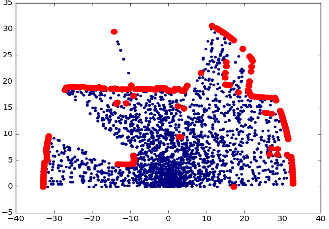

Typically, the objective of occupancy representation is to build a map that can later be used for off-line path planning. Nevertheless, with the requirement of operating robots in real-world environments, it is essential to take dynamics of the environment into account and adjust control policies accordingly. Dynamic occupancy mapping can be categorized into three classes: 1) building static occupancy maps in the presence of dynamic objects, 2) mapping the long-term dynamics of the environment, and 3) mapping the short-term dynamics of the environment. Most of the early research studies on dynamic occupancy mapping fall under the first category in which the dynamic objects are treated as spurious data and remove them to build a robust static map [5, 6, 7, 8]. In the second category, an occupancy pattern is obtained over a long period [5, 9, 10, 11] and such a map can later be used for global path planning. This paper focuses on the third category—mapping short-term dynamics. The short-term dynamics are important not only for understanding the instantaneous changes in the environment but also for making predictions into the future.
To the best of our knowledge, there are only two main techniques to model short-term occupancy and make occupancy predictions into the future. An extension to GPOM, named dynamic Gaussian process (DGP) maps, was proposed in [12] to model the occupancy state of dynamic environments. It proposes a novel covariance function that captures space-time statistical dependencies, thus enabling predictions on future occupancy states. The cubic computational complexity of Gaussian process (GP) classification [13] makes DGPs infeasible in real-time dynamic occupancy mapping. As an alternative, a spatiotemporal extension to HMs (STHMs) was proposed in [14]. This framework uses hinged features to combine temporal variability into the spatial domain modeled by an underlying motion modeling framework.
This paper proposes a novel methodology for spatiotemporal occupancy modeling that builds upon the HM framework, generalizing it to dynamic environments. As shown in Figure 1, the proposed approach can make predictions into the future. Note that the area of uncertainty around the moving vehicle is much larger, due to the increase in uncertainty, which is useful for safely executing motion plans. However, unlike [14], where these dependencies are modeled by a hinged kernel that receives predicted spatial coordinates from a Gaussian process [13], the proposed methodology works by directly updating the feature vector that projects input points into the reproducing kernel Hilbert space (RKHS) [15] for classification, changing its shape to accommodate external motion. A probabilistic dynamic model is incrementally learned for each observed object, using point-cloud alignment techniques on clustered data, and localization uncertainties are also propagated to the occupancy model, accounting for sensor inaccuracies and accumulated drift. The result is an efficient framework capable of tracking multiple 3D objects in real-time, while accurately using this information to probabilistically predict the occupancy state of the environment at arbitrary spatio-temporal resolutions.
The proposed Dynamic Hilbert Maps (DHM) framework also shares similarities with the broader field of dynamic object tracking [16, 17, 18], in the sense that it detects and segments external motion over time. However, while these methods are limited to point-cloud modeling and tracking, ours directly incorporates this information into an incremental occupancy map, which can then be propagated to future or past timesteps to predict the environment at arbitrary resolutions. Additionally, while most dynamic object tracking approaches rely on an initial supervised training stage, either as background filters [19], rigidly attached sample points [20] or deep recurrent neural networks [21], ours is able to build large-scale 3D probabilistic predictive occupancy models without the prior knowledge of similar environments. Although our primary objective is not object tracking, positions and shapes of objects can be easily extracted from DHMs, making DHMs a generalization of object tracking.
II Static Hilbert Maps
Following LARD [2, 22], we define a collection of hinged locations that act as inducing points [23]. With analogy to a multivariate Gaussian shape, these hinged locations have a center alongside another matrix to denote how far the measurements affect in each direction . With the hinged locations , the occupancy probability of any point in the environment can be computed using a logistic model,
| (1) |
with a feature vector defined as:
| (2) | ||||
| (3) |
Learning the model involves two steps. Firstly, the dataset is used to determine the hinge locations using a clustering algorithm [22]. Then, as the crucial step, the parameters are learned by minimizing the objective function of the regularized logistic regression,
| (4) |
where is the norm and are the regularizations weights used to regularize the classifier. is computed similar to (2) by evaluating values. Importantly, since the objective function is represented as a sum of data points, stochastic gradient descent (SGD) [24] can be used.
III Dynamic Hilbert Maps
This section introduces the proposed methodology for dynamic occupancy modeling, that builds upon the Hilbert Maps framework reviewed in Section II. Our objective is to build short-term occupancy maps and make short-term predictions into the future. To accomplish this, three different Hilbert Maps are maintained: , representing the previous timestep; , representing the current timestep; and , representing the accumulated model that is iteratively constructed as more data is collected. We start by describing how to segment objects and calculate motion between timesteps from to , followed by the dynamic model that tracks this motion over time. We then show how to iteratively update the feature vector that defines , modifying the shape of its RKHS to account for external motion. These three steps are discussed below.
III-A Object Segmentation
We assume that, at each timestep , a new pointcloud is obtained, containing sensor data collected at that instant. This pointcloud is clustered to produce , where is the set containing clusters generated from occupied points and contains clusters generated from unoccupied (free) points. We employ the Quick-Means algorithm [25], due to its computational speed and ability to generate similar cluster densities given a resolution threshold . To segment individual objects , where are unique indexes from , only occupied clusters in are considered, as shown in Algorithm 1. Note that the original pointcloud is no longer used, only the extracted clusters , which contributes to a much faster computational time, because . To account for random sensor and environment artifacts, objects with fewer clusters than a certain threshold may be discarded.
III-B Motion Calculation
Once the object set is determined, the next stage is to calculate its motion between timesteps from to . This is done by first calculating the object set , obtained from the cluster set extracted from . To associate between objects from different timesteps we use an overlapping metric, in which each object is associated to the with the closest cluster in its own cluster set:
| (5) |
where and are indexes representing the various clusters that belong respectively to objects and . If the closest cluster is above a certain threshold , that object is considered to have no association with . Similarly, objects in that have no association are considered new (i.e. observed for the first time). Once objects have been associated, motion is estimated using the Iterative Closest Point (ICP) algorithm [26], that minimizes the difference between two pointclouds by calculating the transformation that best matches a source to its target. Following a classical implementation [27], the two-step optimization process described below is adopted, where R is the orthogonal transformation, t is the translation vector and is a rotation group in the -dimensional Euclidean space:
| (6) | ||||
| (7) |
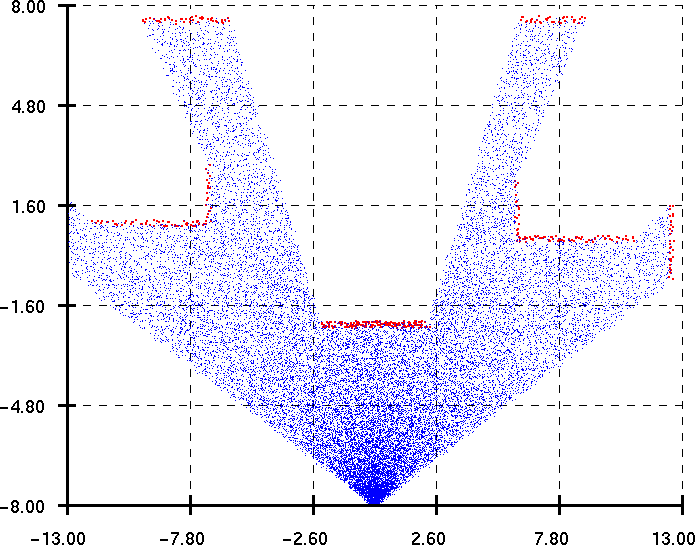
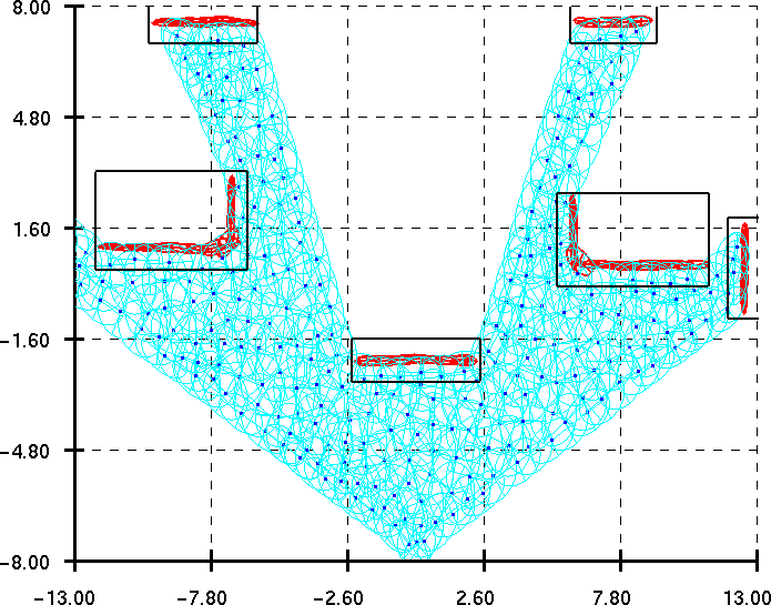
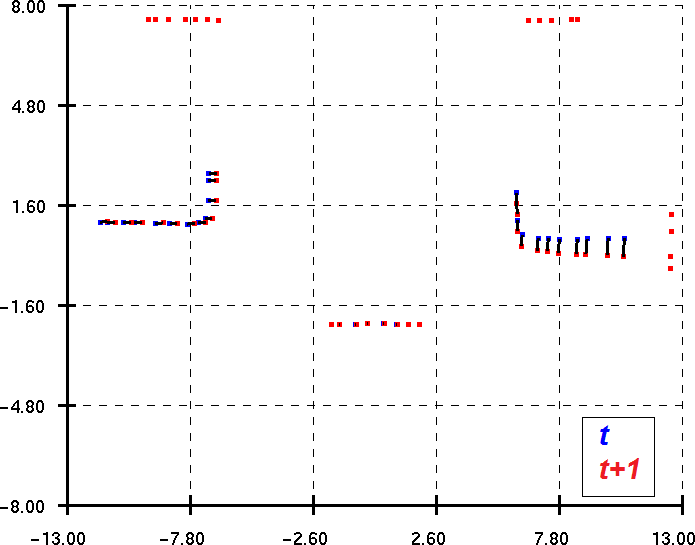
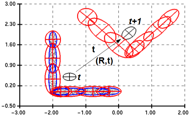
that alternates between computing cluster correspondences from to and solving the optimal rigid transformation that best aligns both sets. In the above equations, is an indicator function that evaluates to if and to otherwise, and is an error function, here selected as the Euclidean norm . Due to a high percentage of outliers and presence of incomplete data, a sparse version of ICP [28] was used during experiments. An example of the proposed method is shown in Figure 2 (a)-(c), where we can see the estimated cluster movement.
III-C Dynamic Object Model
Once the ( transformations are obtained, they can be used to generate the dynamic models that describe object motion over time. These dynamic models allow us to: 1) estimate object position in future (or past) timesteps; 2) incorporate new observations to improve predictions; and 3) account for sensor and model uncertainties. We use a Kalman filter (KF) [29] due to its computational efficiency and closed-form parametric solution, however any other similar technique could be equally applied, such as the Gaussian process regression model from [14].
We start by defining the -dimensional state vector for each object , alongside its covariance matrix (initialized as zero). Note that this state vector includes coordinates and orientation , which is initialized as the direction indicated by the largest eigenvector of (corresponding derivatives, i.e. velocities, are also considered). For each new timestep, the current state of objects is first propagated using the KF Prediction equations:
| (8) | ||||
| (9) |
Afterwards, if a particular object is reobserved, these estimates are refined using the KF Update equations, based on the observation as defined in Equations 6 and 7. Note that a cluster is never truly reobserved, since it is randomly generated from pointcloud data, only its motion based on object alignment:
| (10) | ||||
| (11) |
where is the Kalman gain, with , and is the pre-fit measurement residual. In the above equations, Q and R are respectively the process and observation noise matrices, defined based on system configuration. During experiments, both matrices were defined using cluster resolution, such that , to account for cluster granularity. The matrices F and H are respectively the state transition and observation models, defined as:
| (12) |
where is the interval between timesteps. Even though here we focus on 2D holonomic motion, the described dynamic object model can be trivially extended to 3D navigation.
III-D Feature Vector Updates
Section II described the feature vector used to define the high-dimensional space in which classification takes place within the Hilbert Maps framework. Here we show how this feature vector can be iteratively updated to incorporate motion between timesteps. Instead of constantly retraining the occupancy model to account for dynamic objects, the projective function that defines the RKHS itself is modified, so the same occupancy model is able to naturally describe a changing environment and predict future states.
At where there is no observed motion, an initial occupancy model is generated based on available data (see Section III-A). In subsequent timesteps, the current occupancy model is reassigned as and a new is generated based on newly acquired data, followed by the object segmentation and alignment techniques from Section III-A, relative to . Once alignment is complete, motion from associated objects is calculated according to Section III-B, determining the transformations that propagate different object states from to .
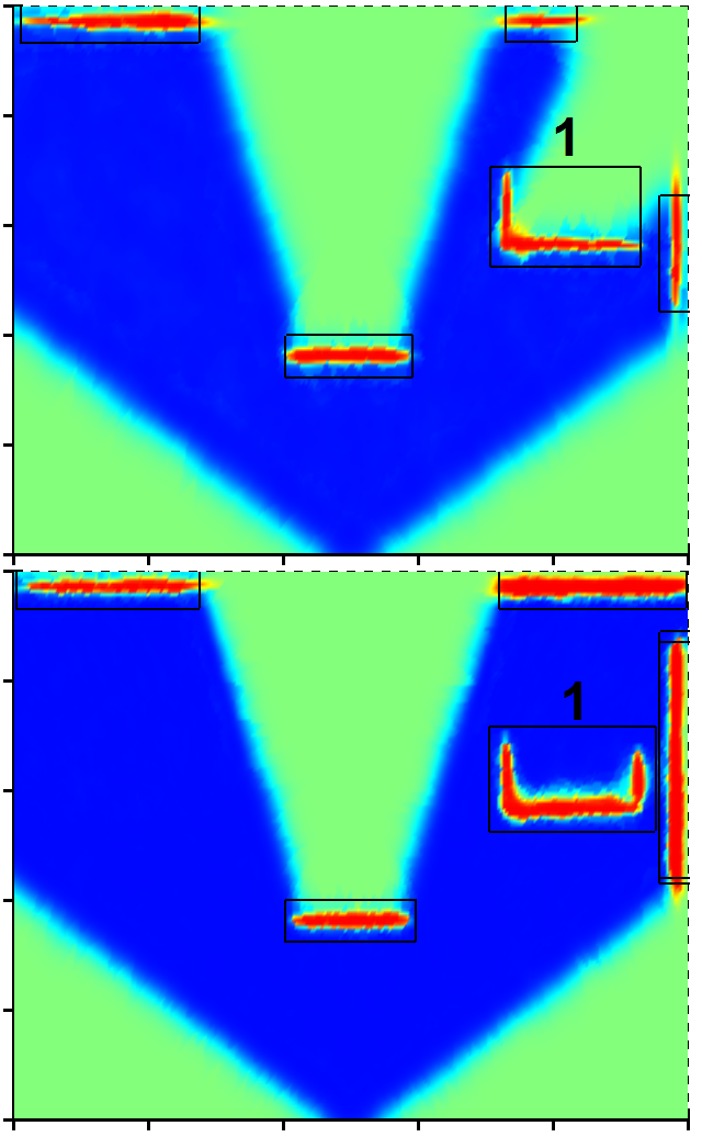
These same transformations are used to propagate object states in from to , as shown in Section III-C. If an object is not reobserved, only the Prediction step is performed (Equations 8 and 9), which leads to an increase in location uncertainty, otherwise the Update step (Equations 10 and 11) also takes place, which decreases location uncertainty values. These state transitions also serve to update the occupied clusters , as depicted in Figure 2 (d), according to the following equations:
| (13) | ||||
| (14) | ||||
| (15) |
As shown above, the contribution parameter for each cluster is also updated, reflecting the decay caused by an increase in location uncertainty. This decay is proportional to the ratio between and , i.e cluster covariance area and sum of cluster and object covariance area. Since these matrices define ellipses, this ratio can be expressed as , where are the eigenvalues of . Intuitively, if (no decay), and as P increases decreases, which indicates a decay in occupancy confidence. Note that, during training and inference, we use as the cluster covariance, so the probabilistic occupancy model also reflects location uncertainty.
Once this time-propagation process is complete, clusters from are selectively incorporated into , as a way to account for newly collected data and to correct alignment errors. Clusters belonging to re-observed objects are added and receive the same dynamic model, while clusters belonging to objects observed for the first time are added with a new dynamic model, initialized to identity states. Similarly, unoccupied clusters are added without a dynamic model (i.e. are considered static). To avoid an unbound increase in cluster number and maintain density roughly constant, only clusters from with nearest neighbor in further than are incorporated. The resulting cluster set defines the new feature vector that projects input data to the RKHS in which operates. Afterwards, is retrained using data from , to produce the current accumulated occupancy model used for inference.
| Time step | Dataset 1 | Dataset 2 | ||||||||
|---|---|---|---|---|---|---|---|---|---|---|
| HM | RSF | DGP | STHM | DHM | HM | RSF | DGP | STHM | DHM | |
![[Uncaptioned image]](/html/1912.02149/assets/figures/fig2d2.png) \captionof
\captionof
figurePlot of Table I, depicting F-Measure scores for different dynamic modeling techniques, for increasing time-steps (Dataset 1).
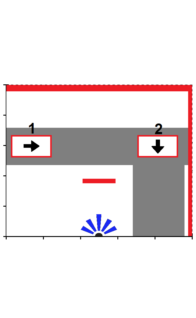
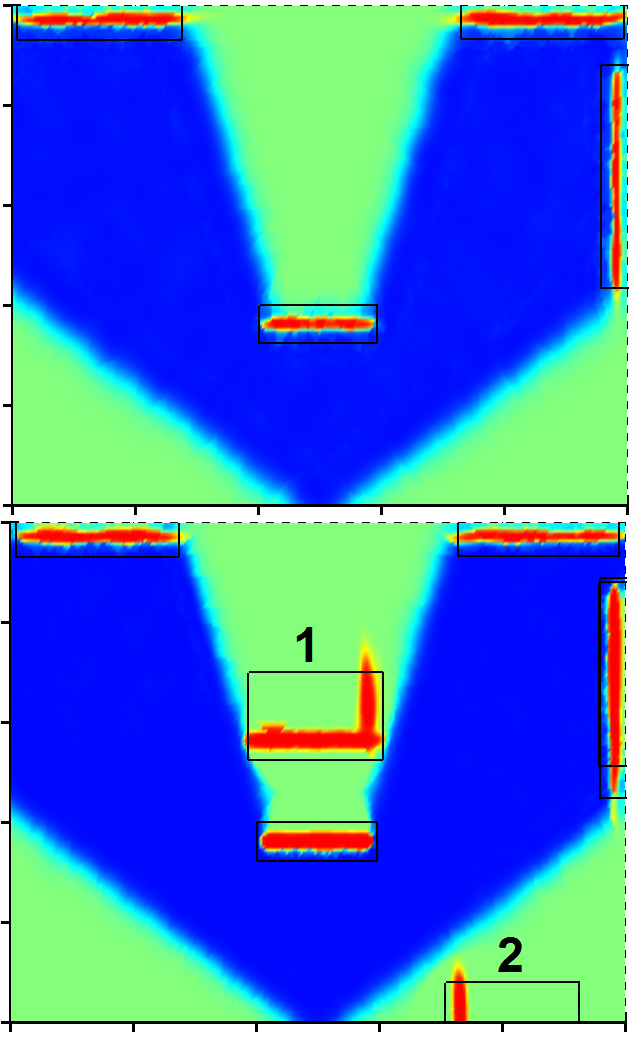
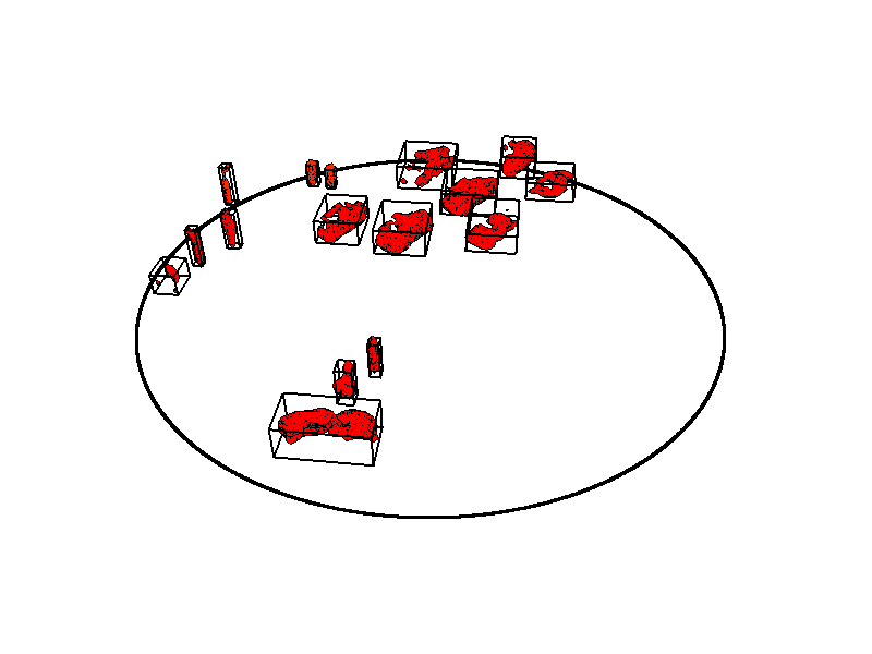
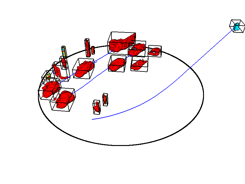
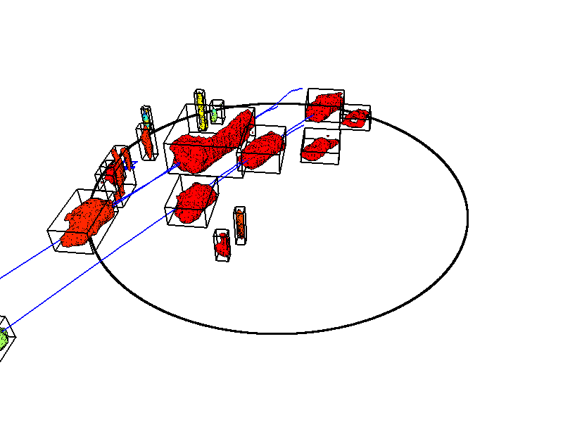
Under the DHM framework, it is possible to query the occupancy anywhere in the space at anytime (past, present, and future). Figure 3 shows an example of the proposed framework, as introduced in this section. At the accumulated and current models are the same, with subsequent time-steps showing how is able to predict the occupancy state of unobserved areas, while taking into account the presence of dynamic objects. Particularly, we can see that, as the same object is observed from different perspectives, this information is incorporated into its dynamic model and used for a full reconstruction in future time-steps. It is also worth noting that static objects are tracked as well (i.e. background walls) and propagated over time, producing a seamless transition between static and dynamic states that is common in real-world applications.
IV Experiments
A series of experiments was performed in order to demonstrate how the proposed methodology, entitled DHM (Dynamic Hilbert Maps), can be applied to the modeling of dynamic environments in both 2D and 3D scenarios. The 2D datasets considered here are the same as in [14], consisting of laser scans collected from a busy urban intersection, covering an angular interval of and varying maximum radii (30m for the first dataset and 100m for the second one). The 3D datasets were obtained from the KITTI Vision Benchmark Suite [30], collected using Velodyne sensors from both static and moving vehicles (GPS + IMU data were used to calculate and compensate ego-motion between timesteps) as they navigate through the streets of urban environments.
IV-A The effect of clustering
As a baseline, initial experiments were performed for the particular case of instant predictions (). In contrast to [14], in which features are hinged randomly or in a regular grid, the proposed methodology uses clustering to produce hinge supports, according to a predetermined cluster resolution . The effects of changing this parameter are shown in Table II, according to different error metrics obtained by randomly sampling timesteps from the first 2D dataset and using the occupancy mapping methodology described in Section II. As expected, the number of clusters decreases as increases, thus producing a more coarse model of observed structures that naturally degrades classification performance. However, a change in resolution from to , with a corresponding increase in computational efficiency of , contributes to a decrease of only in and in , which indicates a low sensitivity to changes in scale that can be used as a trade-off between speed and accuracy. Unless noted otherwise, all further experiments use a cluster resolution value of , which produced the smallest error and highest - score.
| (m) | NC | AUC | NLL | ACC | F-MEAS | TIME |
|---|---|---|---|---|---|---|
IV-B A comparison of dynamic occupancy maps
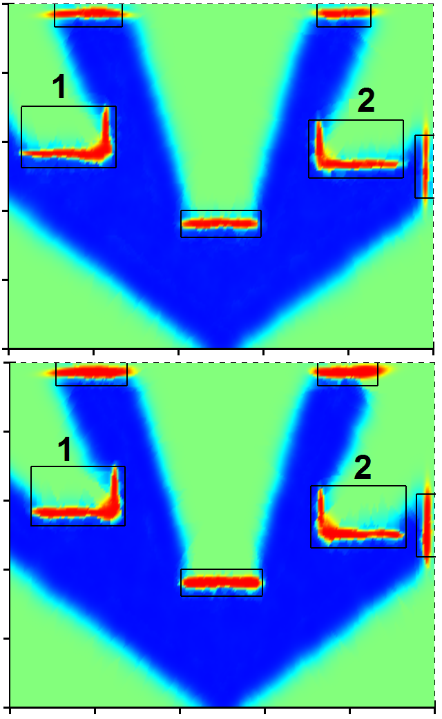
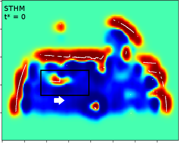
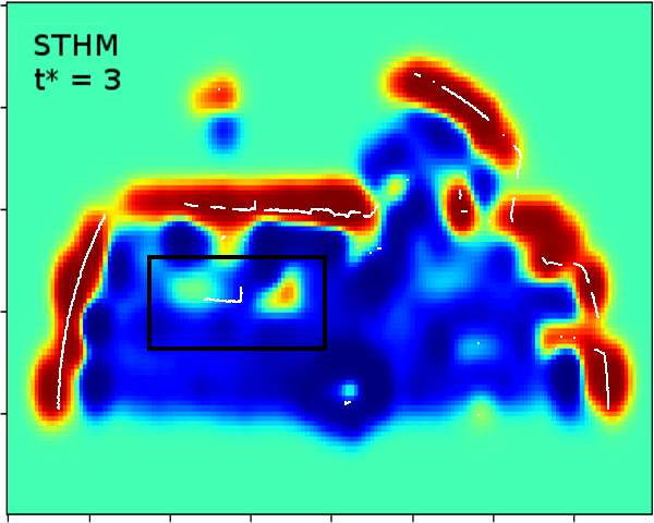
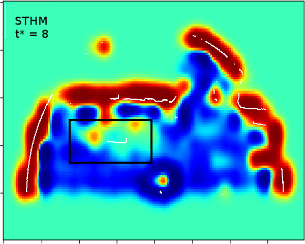
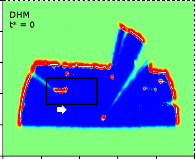
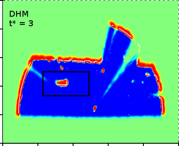
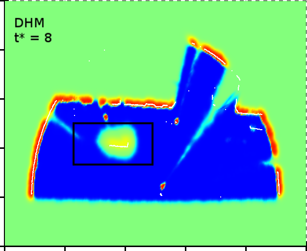
A comparison between different dynamic occupancy modeling techniques, for predictions into future timesteps, is shown in Table I. For all experiments, starting from an empty map, five consecutive frames are used to incrementally learn motion models for the various observed objects, and afterwards predictions are made without incorporating new information. To account for occlusions and the introduction of new objects during prediction, only areas manually annotated as containing dynamic motion (see the black rectangle in Figure 4) are considered, and the F-Measure score is used due to an imbalance between classes, since it encodes both precision and recall values while being less sensitive to uncertainty increase due to weight decay.
As expected, the standard framework, without temporal modeling, quickly degrades in performance due to un-modeled object motion, followed by , that struggles with longer-term predictions. The two HM-based dynamic modeling techniques produce the best F-Measure scores in both datasets, however the proposed consistently outperforms , while maintaining a smoother decrease in performance, mostly due to motion model inaccuracies (i.e. accumulated velocity drift errors) and the propagation of localization uncertainties to occupancy mapping estimates. The algorithm suffers due to its non-probabilistic nature, that is highly sensitive to small calculation errors.
A visual comparison between the two HM-based dynamic modeling techniques is depicted in Figure 4. Note that the proposed technique produces sharper occupancy transitions, due to the clustering process that generates non-stationary kernels for hinge support and having a clear distinction between static and dynamic objects.
IV-C 3D dynamic maps and motion prediction
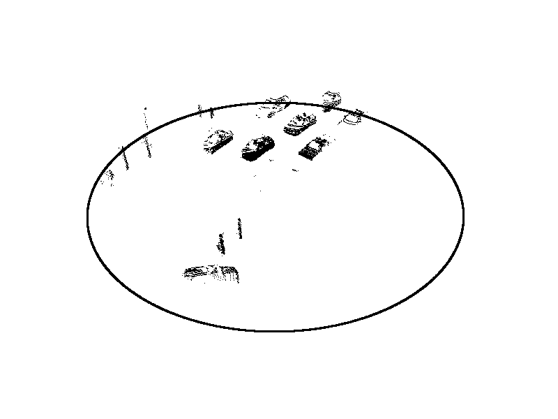
Similar experiments were also performed using 3D datasets (Figure 5), with results depicted in Table III. Only , the standard framework and the proposed technique were considered, since other techniques do not scale favorably to higher dimensions ( scales cubically with the number of training points and maintains a regular grid throughout the entire input space). In contrast, updates between timesteps require roughly ms and ms in 2D and 3D datasets111All computations were performed on a i7/2.608 GHz notebook, with multi-threading enabled wherever possible. A C++ demo is available at https://bitbucket.org/vguizilini/cvpp, respectively, which makes it applicable to online tasks under real-time constraints. Interestingly, the proposed technique achieved better overall results for longer-term predictions when using 3D data, most likely due to a richer pointcloud representation of structures, that facilitates ICP alignment and thus produces better motion models. Additionally, it is worth noting that the introduction of a moving sensor for data collection did not significantly impact performance.
V Conclusion
This paper introduces a novel technique for dynamic occupancy mapping that efficiently incorporates temporal dependencies between data collected in different time-steps. Under this framework, new observations are used to learn a global accumulation map. This enables seamlessly generating future occupancy maps even in the presence of occlusions. Considering both runtime and accuracy, the proposed framework outperforms state-of-the-art dynamic mapping techniques as tested using 2D and 3D datasets. Future work will focus on different motion models for tracking more complex patterns and improving data association between objects.
| Time step | Static Sensor | Moving Sensor | ||||
|---|---|---|---|---|---|---|
| (m) | HM | RSF | DHM | HM | RSF | DHM |
ACKNOWLEDGMENT
This research was supported by funding from the Faculty of Engineering & Information Technologies, The University of Sydney, under the Faculty Research Cluster Program.
References
- [1] A. Elfes, “Occupancy grids: A probabilistic framework for robot perception and navigation,” Ph.D. dissertation, Carnegie Mellon University, Pittsburgh PA, USA, 1989.
- [2] F. Ramos and L. Ott, “Hilbert maps: Scalable continuous occupancy mapping with stochastic gradient descent,” in Proceedings of Robotics: Science and Systems (RSS), 2015.
- [3] K. Doherty, J. Wang, and B. Englot, “Bayesian generalized kernel inference for occupancy map prediction,” in Robotics and Automation (ICRA), 2017 IEEE International Conference on. IEEE, 2017, pp. 3118–3124.
- [4] ——, “Probabilistic map fusion for fast, incremental occupancy mapping with 3d hilbert maps,” in Robotics and Automation (ICRA), 2016 IEEE International Conference on. IEEE, 2016, pp. 1011–1018.
- [5] D. Meyer-Delius, M. Beinhofer, and W. Burgard, “Occupancy Grid Models for Robot Mapping in Changing Environments,” in AAAI Conference on Artificial Intelligence (AAAI), 2012.
- [6] D. Hahnel, R. Triebel, W. Burgard, and S. Thrun, “Map building with mobile robots in dynamic environments,” in IEEE International Conference on Robotics and Automation (ICRA), 2003, pp. 4270–4275.
- [7] C. Stachniss and W. Burgard, “Mobile robot mapping and localization in non-static environments,” in aaai, 2005, pp. 1324–1329.
- [8] D. Nuss, R. Stephan, M. Thom, T. Yuan, K. Gunther, M. Michael, G. Axel, and K. Dietmayer, “A random finite set approach for dynamic occupancy grid maps with real-time application,” in arXiv preprint arXiv:1605.02406, 2016.
- [9] T. Krajnık, P. Fentanes, G. Cielniak, C. Dondrup, and T. Duckett, “Spectral analysis for long-term robotic mapping,” in IEEE International Conference on Robotics and Automation (ICRA), 2014, pp. 3706–3711.
- [10] R. Senanayake, S. O’Callaghan, and F. Ramos, “Learning highly dynamic environments with stochastic variational inference,” in IEEE International Conference on Robotics and Automation (ICRA), 2017.
- [11] R. Senanayake and F. Ramos, “Bayesian hilbert maps for dynamic continuous occupancy mapping,” in 1st Annual Conference on Robot Learning (CoRL), 2017.
- [12] S. O’Callaghan and F. Ramos, “Gaussian process occupancy maps for dynamic environments,” in Experimental Robotics. Springer Tracts in Advanced Robotics, 2015, vol. 109, pp. 791–805.
- [13] C. Rasmussen and C. Williams, Gaussian Processes for Machine Learning. The MIT Press, 2005.
- [14] R. Senanayake, L. Ott, S. O’Callaghan, and F. Ramos, “Spatio-temporal Hilbert maps for continuous occupancy representation in dynamic environments,” in Advances in Neural Information Processing Systems (NIPS), 2016.
- [15] B. Schölkopf and A. Smola, Learning with Kernels: Support Vector Machines, Regularization, Optimization, and Beyond. The MIT Press, 2001.
- [16] D. Wang, “Laser-based detection and tracking of dynamic objects,” Ph.D. dissertation, Mobile Robotics Group, University of Oxford, October 2014.
- [17] D. Held, J. Levinson, S. Thrun, and S. Savarese, “Combining 3d shape, color and motion for robust anytime tracking,” in Proceedings of Robotics: Science and Systems (RSS), 2014.
- [18] A. Dewan, T. Caselitz, G. Tipaldi, and W. Burgard, “Rigid scene flow for 3d lidar scans,” in Proceedings of the IEEE International Conference on Intelligent Robots and Systems (IROS), 2016.
- [19] A. Ushani, R. Wolcott, J. Walls, and R. Eustice, “A learning approach for real-time temporal scene flow estimation from lidar data,” in Proceedings of the IEEE International Conference on Robotics and Automation (ICRA), 2017.
- [20] D. Zeng, I. Posner, and P. Newman, “Model-free detection and tracking of dynamic objects with 2d lidar,” International Journal of Robotics Research (IJRR), 2015.
- [21] J. Dequaire, P. Ondruska, D. Rao, D. Wang, and I. Posner, “Deep tracking in the wild: End-to-end tracking using recurrent neural networks,” International Journal of Robotics Research (IJRR), 2017.
- [22] V. Guizilini and F. Ramos, “Large-scale 3d scene reconstruction with Hilbert maps,” in Proceedings of the IEEE International Conference on Intelligent Robots and Systems (IROS), 2016.
- [23] E. Snelson and Z. Ghahramani, “Sparse Gaussian processes using pseudo-inputs,” in Advances in Neural Information Processing Systems (NIPS), 2006, pp. 1257–1264.
- [24] L. Bottou, “Large-scale machine learning with stochastic gradient descent,” in Proceedings of COMPSTAT’2010. Springer, 2010, pp. 177–186.
- [25] V. Guizilini and F. Ramos, “Learning to reconstruct 3d structures for occupancy mapping,” in Proceedings of Robotics: Science and Systems (RSS), 2017.
- [26] F. Pomerleau, F. Colas, and R. Siegwart, “A review of point cloud registration algorithms for mobile robotics,” Foundations and Trends in Robotics, vol. 4, no. 1, pp. 1–104, 2015.
- [27] A. Segal, D. Haehnel, and S. Thrun, “Generalized icp,” in Proceedings of Robotics: Science and Systems (RSS), 2009.
- [28] S. Bouaziz, A. Tagliasacchi, and M. Pauly, “Sparse iterative closest point,” in Computer Graphics Forum (Symposium on Geometry Processing, vol. 32, no. 5, 2013, pp. 1–11.
- [29] G. Welch and G. Bishop, “An introduction to kalman filter,” University of North Carolina at Chapel Hill, Tech. Rep., 1995.
- [30] A. Geiger, P. Lenz, C. Stiller, and R. Urtasun, “Vision meets robotics: The kitti dataset,” International Journal of Robotics Research (IJRR), 2013.
- [31] C. Bishop, Pattern Recognition and Machine Learning (Information and Statistics. Springer-Verlag New York, Inc., 2006.
- [32] W. Lorensen and H. Cline, “Marching cubes: A high resolution 3d surface construction algorithm,” in Proceedings of the Annual Conference on Computer Graphics and Interactive Techniques (SIGGRAPH), vol. 14, 1987, pp. 163–169.