Saturn’s Probable Interior: An Exploration of Saturn’s Potential Interior Density Structures

Abstract

The gravity field of a giant planet is typically our best window into its interior structure and composition. Through comparison of a model planet’s calculated gravitational potential with the observed potential, inferences can be made about interior quantities, including possible composition and the existence of a core. Necessarily, a host of assumptions go into such calculations, making every inference about a giant planet’s structure strongly model dependent. In this work we present a more general picture by setting Saturn’s gravity field, as measured during the Cassini Grand Finale, as a likelihood function driving a Markov-Chain Monte Carlo exploration of the possible interior density profiles. The result is a posterior distribution of the interior structure that is not tied to assumed composition, thermal state, or material equations of state. Constraints on interior structure derived in this Bayesian framework are necessarily less informative, but are also less biased and more general. These empirical and probabilistic constraints on the density structure are our main data product which we archive for continued analysis. We find that the outer half of Saturn’s radius is relatively well constrained, and we interpret our findings as suggesting a significant metal enrichment, in line with atmospheric abundances from remote sensing. As expected, the inner half of Saturn’s radius is less well-constrained by gravity, but we generally find solutions that include a significant density enhancement, which can be interpreted as a core, although this core is often lower in density and larger in radial extent than typically found by standard models. This is consistent with a dilute core and/or composition gradients.

[pdftoc]hyperrefToken not allowed in a PDF string [rerun]rerunfilecheck [labels]latexLabel(s) may have changed. [sfloat]latexA float is stuck [dfloat]revtex4-1Deferred float stuck [pdftoc,rerun,labels,sfloat,dfloat]

1 Introduction

1.1 The Gravity Field as a Probe on the Interior

There are a number of fundamental questions that we would like to understand about giant planets. Do they have a heavy element core? If so, what is its mass? Is it distinct from the overlying H/He envelope, or partially mixed into it? Is the H/He envelope enriched in heavy elements compared to the Sun? Is the envelope fully convective and well mixed?

Unfortunately, the vast mass of a giant planet is completely hidden from view, so that we must use indirect methods to try to answer these questions. Most of our knowledge about the interiors of giant planets comes from interpreting their gravity fields, as recently reviewed for Saturn by Fortney et al. (2018). Since the planets are fluid and rapidly rotating they assume an oblate shape and their gravitational potential differs from that of a spherically symmetric body of the same mass. The external gravitational potential $V_{\text{e}}$ is a function of the colatitude $\theta$ and distance $r$ from the center of the planet, and is typically written as an expansion in powers of $R_{\text{eq}}/r$ where $R_{\text{eq}}$ is the equatorial radius of the planet:

$$V_{\text{e}}(r,\theta)=-\frac{GM}{r}\left(1-\sum_{n=1}^{\infty}(R_{\text{eq}}/r)^{n}J_{n}P_{n}(\cos\theta)\right).$$ (1)

In eq. (1) $P_{n}$ are Legendre polynomials of degree $n$. The coefficients $J_{n}$ (“the Js”) are measurable for many solar-system bodies by fitting a multi-parameter orbit model to Doppler residuals of spacecraft on close approach. For fluid planets in hydrostatic equilibrium, where azimuthal and north-south symmetry holds, only even-degree coefficients are non-zero.

When an interior model for a planet is created, the $J_{n}$ values are calculated as integrals of the interior density over the planetary volume:

$$MR_{\text{eq}}^{n}J_{n}=-\int\rho(\mathbf{r^{\prime}})(r^{\prime})^{n}P_{n}(\cos\theta^{\prime})\,d\tau^{\prime}.$$ (2)

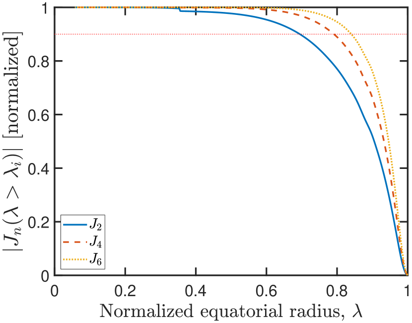
These model $J_{n}$ can then be compared to measured ones. As is well-known, the different Js sample the density at different depths (with $J_{2}$ probing deepest) but with significant overlap, and with most of the weighting over the planet’s outer half in radius. This point is illustrated in Figure 1.

Figure 1: Contribution functions of the gravitational harmonics $J_{2}$ (blue solid), $J_{4}$ (red dashed), $J_{6}$ (yellow dotted) for a typical, 3-layer Saturn model. The contribution “density” ($\propto{}J(r)dr$) is plotted in the left panel and the cumulative contribution in the right panel. The horizontal line intersects the curves at a depth where the corresponding $J$ reaches 90% of its final value.

The gravity field is a non-unique feature of the interior mass distribution. In other words, different mass distributions can lead to identical gravity signals. This complicates the process of making inferences about the interior structure based only on the external gravity field. In principle, one should explore a wide range of possible interior structures, of possible $\rho(\mathbf{r^{\prime}})$ in eq. (2), to see the full range of solutions that fit the gravity field. Initially, researchers had focused on finding a single, best-fit solution subject to a host of assumptions, chosen for computational convenience and not necessarily following reality. More recently there have been efforts to explore an expanded range of interior structures, usually by making alternative assumptions about the prototypical planet.

The main contribution of the present work is the introduction of a different approach to the task of inferring interior structure from gravity, and the application of this approach to Saturn. The result is a suite of interior structure models of Saturn computed with fewer assumptions and therefore showing a fuller range of structures consistent with observation. We describe our method in detail and compare it with previous work of similar spirit in sec. 1.2.4 and 2.6.

1.2 Common Assumptions in planetary interior models

There are typically at least three significant assumptions or choices that modelers make when constructing interior models of giant planets, thereby implicitly constraining the possible inferences from these models.

1.2.1 The planets have three layers

Perhaps the most constraining assumption is the prototypical picture of three layers, each well-mixed enough to be considered homogeneous. For Jupiter and Saturn these are a Helium-poor outer envelope, a Helium-rich inner envelope, and a heavy-element, usually constant density core. Investigators also adjust the abundance of heavy elements in the He-rich and He-poor layers, with little physical motivation other than it seems to facilitate finding an acceptable match to the gravity field.

While a core-envelope structure is certainly a plausible one, and indeed rooted in well studied planet formation theories, the assumption of compositionally homogeneous layers may well be a significantly limiting oversimplification.

1.2.2 The interior pressure-temperature profile is isentropic

A typical assumption of interior modeling is that pressure-temperature profile is isentropic, lying on a single $(P,T)$ adiabat that is continued from a measured or inferred temperature at 1 bar. This second assumption is likely to be true over some of the interior, but there are good reasons to doubt that this holds throughout the interior.

Jupiter and Saturn have an atmospheric He depletion compared to the Sun, and it has long been suggested that this is due to He phase separation from liquid metallic hydrogen in the deep interiors (Stevenson & Salpeter, 1977; Fortney & Hubbard, 2003). There is likely a region with a He abundance gradient starting between 1 to 2 Mbar in both planets (Nettelmann et al., 2015; Mankovich et al., 2016). In models that attempt to interpret the gravity field, if such a layer is included at all it is by interpolation between outer and inner homogeneous layers (e.g. Wahl et al., 2017; Militzer et al., 2019), but this interpolation is unlikely to capture fully the effects of composition gradients. Composition gradients can inhibit large scale convection (Ledoux, 1947) implying that heat is transported via layered convection or radiation/conduction. This leads to higher internal temperatures that in return allow higher heavy-element enrichment at a given density-pressure. Indeed, non-adiabatic structures have been recently suggested for all outer planets in the solar system (e.g. Leconte & Chabrier, 2012; Vazan et al., 2016; Podolak et al., 2019).

1.2.3 The inferred composition relies on equation of state calculations

As the field progresses the equations of state (EOS) used for modeling giant planet interiors become a better representation of reality. Nevertheless, the equations of state for all the relevant materials and mixtures are not perfectly known. Simulations from first principles of hydrogen, helium, and their mixtures over the conditions relevant for giant planets have been carried out and partially validated against experimental data (Nettelmann et al., 2008; Militzer & Hubbard, 2013). These equations of state (EOSs) for hydrogen show good agreement with data up to $\sim\!\!{1.5\;\mathrm{Mbar}}$ (e.g. Militzer et al., 2016). However, the pressure at the bottom of Saturn’s H/He envelope is about 10 Mbar and for Jupiter it is about 40 Mbar, well beyond the realm of experiment. Recent structure models used EOS for hydrogen and helium based on Density Functional Theory (DFT) simulations (Militzer et al., 2016; Nettelmann et al., 2008; Miguel et al., 2016). Until recently, different EOS led to different inferred compositions for Jupiter due to different approaches to calculating the entropy. Today, there is good agreement between state-of-the-art EOSs (Nettelmann, 2017), but it should be kept in mind that DFT also suffers from approximations (Mazzola et al., 2018) and there remains an uncertainty of $\sim\!\!{2\%}$ in the hydrogen EOS, which increases significantly when it comes to predicting hydrogen-helium demixing (Morales et al., 2009).

The heavy elements must also be represented by an EOS (typically for water or silicates) which introduces another source of uncertainty. Therefore, the range of possible composition and internal structure from such interior models cannot be taken to be the true range of allowed values, even if the parameter space of possible EOSs, H/He/Z mixing ratios, and outer/inner envelope transition pressures were thoroughly explored.

1.2.4 Appreciating the complexities

The drawbacks of the assumptions discussed above have long been known and the reality that giant planets are surely more complicated than the traditional modeling framework allows for is generally accepted (e.g., Stevenson, 1985). More recent investigations are attempting to allow for a more complex structure. Interior composition gradients due to remnants of formation (Leconte & Chabrier, 2012; Helled & Stevenson, 2017), core dredge-up (Militzer et al., 2016), convective mixing of primordial composition gradients (Vazan et al., 2016, 2018), and He sedimentation (Nettelmann et al., 2015; Mankovich et al., 2016) have been considered and were found to lead to different structures. Additionally, some investigators have begun using what may be referred to as “empirical” models. In this context an empirical model is one that is focused on the more direct connection between gravity and density (e.g. Helled et al., 2009) or gravity and equilibrium shape (Helled et al., 2015), without invoking the compositional and thermodynamical origin of these structures.

The work we present here is in the spirit of empirical models. We explore systematically, in a Bayesian inference framework, the possible density profiles of Saturn. We limit our assumptions as much as possible, in order to find the widest range of interior structures with their probability distribution based on their gravitational potential matching the observed field.

2 Composition-independent interior density calculation

The premise of removing some assumptions and deriving composition-free interior density profiles (sometimes referred to as empirical models) is simple and in fact has been pursued in previous work (e.g., Marley et al., 1995; Podolak et al., 2000; Helled et al., 2009). (We discuss similarities and differences with these works in sec. 2.6 below.) The only information that is needed to calculate a gravity field is the density everywhere inside the planet, $\rho(\mathbf{r})$, and so this is the only quantity we will directly vary. In fact, hydrostatic equilibrium produces level surfaces, closed surfaces of constant density, pressure, and potential, and therefore a one-dimensional description of the mass distribution is sufficient: we can use $\rho(\mathbf{r})=\rho(s)$ where $s$ is the volumetric mean radius of the unique level surface of density $\rho$.

All other properties of the planet will be inferences, rather than input parameters. Since there is unavoidable uncertainty associated with the measurement of the gravity field (and also with its theoretical calculation from interior models; see 2.4), this means that there must be a continuous distribution of possible density profiles that fit the gravity solution, and we must base our inferences on the entire distribution. In practice, since we can only ever consider a finite number of solutions, this means that we must base our inferences on a random sample from this unknown distribution of allowed solutions.

In this section we describe the process of obtaining this random sample, as applied to Saturn. For the most part the same process would apply equally well to the other giant planets. We mention in places modifications that may be needed if the same method is to be applied to Jupiter, Uranus, or Neptune.

2.1 Overview

Formally, the distribution we are after is the posterior probability $p(\boldsymbol{\rho}|\mathbf{J}^{\star})$, the probability that the planet’s interior density follows $\boldsymbol{\rho}=\rho(s)$ given that the gravity coefficients were measured as $\mathbf{J}^{\star}$. This consists of several subtasks. First we must find a suitable parameterization of $\rho(s)$. This parameterization should be able to represent all the physically reasonable $\rho(s)$ curves without undue loss of generality, but this is not particularly difficult. It is also necessary that the range and behavior of the numeric values of all parameters is such that they can be efficiently sampled, e.g., with a Markov Chain Monte Carlo (MCMC) algorithm. This is easier said than done, and the best parameterization may be different for different planets.

For Saturn we find that a piecewise-quadratic function of density as a function of normalized radius works best for the bulk of the planet, with a quartic (degree 4) polynomial required to represent the uppermost region (for $P\lesssim{2}\;\mathrm{GPa}$). We describe this parameterization in detail in section 2.2. Note that this is one place where modifications might be needed before applying the same procedure to Jupiter or the ice giants.

To drive the sampling algorithm we need a way to evaluate the relative likelihood of two model planets and we do this by comparing how well they match Saturn’s observed mass and gravity field. The details of this calculation are given in section 2.3.

The likelihood calculation requires that we know the equilibrium shape and gravity field of a given density profile, to sufficient accuracy. Note that in eq. (2) the integrand is known but the integration bounds are unknown. We need to first determine the planet’s equilibrium shape. The shape is determined by a balance between the centrifugal acceleration of the rotating planet and the gravitational acceleration. This is therefore a circular problem, requiring an iterative calculation to converge to a self-consistent solution.

We use an implementation of $4^{th}$-order Theory of Figures (ToF) using the coefficients given in Nettelmann (2017) and employ optimization techniques that allow us to solve the hydrostatic equilibrium state to desired precision very quickly. The details are given below in the section 2.4.

The emphasis on speed is necessary, as the next subtask is to employ a suitable MCMC algorithm to draw a large sample of possible $\boldsymbol{\rho}$. There is no generally agreed upon method of predicting the number of sampling steps required for convergence. By experimentation we find that our Saturn parameterization requires tens of thousands of steps to become independent of its seed state and has a long auto-correlation time, requiring a large number of steps following convergence to obtain the desired effective sample size. Producing a valid sample required the computation of about ten million model planets in total. We give the details of our sampling method and convergence tests in sec 2.5  C.

The last step is calculating some derived physical quantities of interest, based on the obtained $\boldsymbol{\rho}$ sample. Given the gravity field, the pressure on each level surface can be computed from the hydrostatic equilibrium equation. And with knowledge of the pressure and density at each level we may begin to estimate other quantities of interest, e.g., the helium fraction, the heavy element content, etc. These quantities are not determined directly by the gravity field but can be inferred, with additional assumptions. We discuss the results of this analysis, as applied to Saturn, in section 3.

2.2 Parameterization of $\rho(s)$

Our goal is to sample from a space of $\rho(s)$ curves that is as general as possible, making a minimum of assumptions about $\rho(s)$ while still restricting the sample to physically meaningful density profiles and, importantly, keeping the number of free parameters small, for sampling efficiency. These competing requirements are not easy to satisfy and it may be that the best parameterization depends on the planet being studied as well as on the available sampling algorithms and computing resources.

When looking for a good parameterization of $\rho(s)$ we were guided by previously published work on Saturn’s interior. Traditionally derived models are less general than we would like but they are physically sound. Examining them exposes the major features expected of a $\rho(s)$ curve representing Saturn’s interior. Figure 2 shows the density profiles of several Saturn models recently published by Mankovich et al. (2019, hereafter M19).

Figure 2: Three representative Saturn density profiles from M19. These profiles were derived using the standard, three-layer assumption, and thus represent only a subset of possible profiles. On the other hand they are known to be in strict agreement (by construction) with theoretical EOS throughout the interior. The inset shows a zoomed-in view of the top part of the envelope. The red solid line is the same curve as in the full scale figure; the black dotted line is a quadratic fit, a good approximation of the upper envelope overall, and the blue dashed line is a quartic fit to the segment $s/R_{\text{m}}>0.94$, a much better fit there (appendix A).

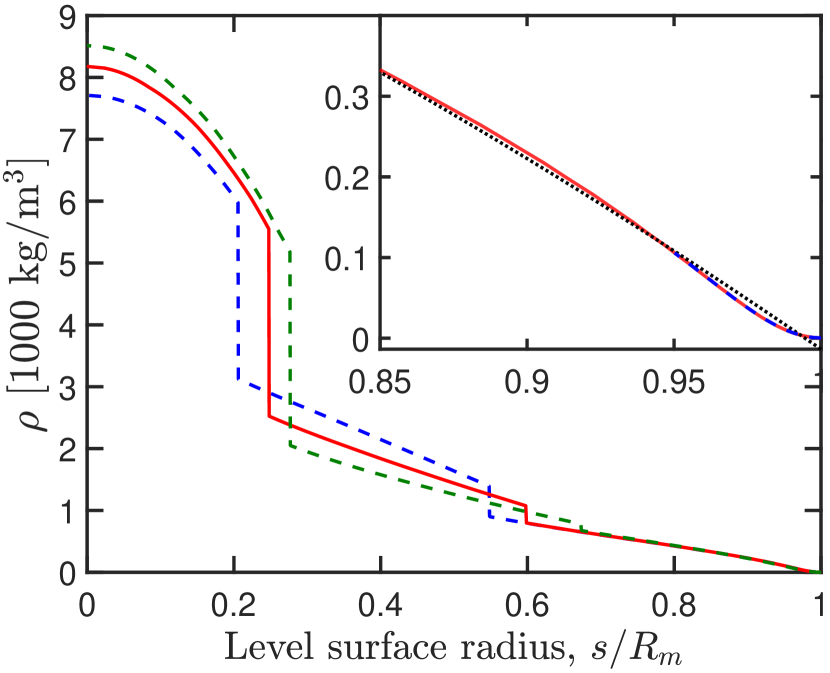
The general feature is a monotonic and piecewise-smooth function in three segments. This is not surprising, as these models were all derived with the assumption of three layers of homogeneous composition, commonly thought of as an upper envelope, lower envelope, and core. While we do not wish to make such a strong assumption, we find it necessary to make the much weaker assumption that $\rho(s)$ is a monotonic, piecewise-smooth function, with no more than (but possibly fewer than!) two density discontinuities. Further, between discontinuities the density appears to follow very smooth curves, suggesting that it may be well approximated by a quadratic function of $s/R_{m}$ for each segment, where $R_{\text{m}}=58232\;\mathrm{km}$ is Saturn’s volumetric mean 1-bar radius . By experimentation, we find no advantage in using higher order polynomials to approximate any of the main segments.

This piecewise-continuous model should not be confused with the traditional 3-layer one. The density being piecewise continuous is a much less strict assumption than the composition being piecewise constant, even if they lead to visually similar plots. Nevertheless, it would be even better to allow more discontinuities or, better yet, a variable number of them. While this may seem like a relatively straightforward generalization, it would in fact greatly increase the computational cost of sampling the parameter space. To understand why consider that each additional discontinuity in $\rho(s)$ not only introduces four additional parameters (the three parameters required to describe the quadratic plus the location of the additional break point), these parameters will also be highly correlated with the rest. As it turns out, this correlation is already evident with just two discontinuities. Informally, each of the two density “jumps” can substitute for the other in the large subset of models where only a single pronounced discontinuity appears. This evident “redundancy” is by no means proof that there cannot be more than two sharp density jumps in Saturn’s interior. But it helps us accept, at least temporarily, a compromise between maximum generality and minimum CPU hours.

It is important to note that to date all EOS-based models of Saturn find solutions consistent with the measured gravity field that predict a concentration of heavy elements in the envelope of at most a few times the protosolar value (e.g. Nettelmann et al., 2013; Helled & Guillot, 2013; Militzer et al., 2019) while Saturn’s atmospheric spectra indicate a higher value, perhaps as high as 10 times the protosolar metallicity (Atreya et al., 2016). In principle, atmospheric enrichment might not represent the bulk composition of the outer envelope, as was recently suggested for Jupiter (Debras & Chabrier, 2019). Nevertheless this demonstrates that, while we wish to be guided by physical models, our parameterization must not be overly constrained by them.

To summarize, we arrive at the following parameterization, using $z=s/R_{\text{m}}$:

$$\rho(z)=\begin{cases}\rho\bigl{(}z,[\mathbf{q}_{1},\mathbf{q}_{2},\mathbf{q}_{3},z_{1},z_{2}]\bigr{)},&0<z<z_{a}\\ \rho\bigl{(}z,[\mathbf{Q}(\rho_{a})]\bigr{)},&z_{a}<z<1.\end{cases}$$ (3)

Here $\mathbf{q}_{1}$ are the three parameters defining the first (outermost) quadratic segment, $\mathbf{q}_{2}$ are the three parameters defining the second (middle) quadratic segment, and $\mathbf{q}_{3}$ are the three parameters defining the third (deepest) quadratic segment. The transition between the first and second segments is at normalized radius $z_{1}$ (which we let vary from 0.35 to 0.9 in normalized radius) and the transition between the second and third segments is at $z_{2}<z_{1}$ (which we let vary from 0.1 to 0.4). The quartic segments are uniquely determined by the density at $z_{a}$, itself already determined by the coefficients $\mathbf{q}_{1}$. We thus have 11 free parameters – three each for the three quadratic segments, plus the two “floating” transition radii.

2.3 Comparing model and observation

MCMC sampling works by comparing, at every iteration, the likelihood of a proposed vector of parameter values, $L(\mathbf{y})$, with that of the current vector of parameter values, $L(\mathbf{x})$, and accepting or rejecting the proposed values with probability proportional to the relative likelihoods. If the likelihood function is itself proportional to the desired (unknown) posterior probability, in our notation, if $L(\mathbf{x})\propto{}p\bigl{(}\boldsymbol{\rho}(\mathbf{x})|\mathbf{OBS}\bigr{)}$, then the resulting Markov chain will converge, in the long run, to a sample from that posterior. For $\mathbf{OBS}$ we substitute any number of observed quantities that may differ from those calculated in the model.

A likelihood function that is proportional to the desired posterior is the function $L(\mathbf{x})=p\bigl{(}\mathbf{OBS}|\boldsymbol{\rho}(\mathbf{x})\bigr{)}p\bigl{(}\mathbf{x}\bigr{)}$. It is proportional to the posterior as a consequence of Bayes’ rule. The prior probability $p(\mathbf{x})$ is necessary. It is our informed, subjective assessment of what values the model parameters $\mathbf{x}$ are expected to take, and typically it is a simple product of the individual prior probabilities of the independent variables $x_{i}$, which in turn are either uniform or normal inside a region of reasonable values. What we need then is to provide the MCMC algorithm with a function that evaluates the relative goodness of the match between the observed properties of the planet and the values of the same properties as calculated for the model, taking uncertainties from both model and observation into account.

In this context the planetary properties that our models need to match are the gravity coefficients $\mathbf{J}^{\star}$ and the planet’s mass $M_{\text{Sat}}$.

First, the gravity. We assume that the observed values $\mathbf{J}^{\star}{}$ are normally distributed about the true, unknown, mean values, and calculate a distance:

$$D_{J}^{2}=\left(\frac{J_{2}-J^{\star}_{2}}{\sigma_{J_{2}}}\right)^{2}+\left(\frac{J_{4}-J^{\star}_{4}}{\sigma_{J_{4}}}\right)^{2}+\left(\frac{J_{6}-J^{\star}_{6}}{\sigma_{J_{6}}}\right)^{2},$$ (4)

where the $\sigma_{J_{i}}$ are measures of the uncertainty in either the measured or the computed values, or both.

In the work presented here only $J_{2}$, $J_{4}$, and $J_{6}$ were considered for the purpose of calculating the likelihood function. Higher order coefficients $J_{8}$–$J_{12}$, as well as non-vanishing odd-indexed coefficients $J_{3}$ and $J_{5}$, have been measured for Saturn, to impressive precision, by the Cassini Grand-Finale gravity experiment (Iess et al., 2019). But it seems clear that these reflect an increasingly large contribution from an asymmetric and/or time-varying field, deriving either from planet-scale differential rotation or from deeply rooted zonal winds, or both (Galanti & Kaspi, 2017; Kaspi et al., 2018; Galanti et al., 2019; Iess et al., 2019). These phenomena are important in themselves and offer a promising avenue for studying further Saturn’s dynamic nature, but for the purpose of constraining the bulk interior structure their net result is to increase the effective uncertainty of the low-order Js ascribed to solid-body rotation (Guillot et al., 2018). Studies of differential rotation on Saturn demonstrate that their contribution to the low-order even harmonics can be significant (Hubbard, 1982; Galanti & Kaspi, 2017). As our goal is to capture the widest range of probable interior structures, we compute eq. (4) for every model by assuming solid-body rotation and setting $J^{\star}_{2}=16290.573\times{10}^{-6}$, $J^{\star}_{4}=-935.314\times{10}^{-6}$, and $J^{\star}_{6}=86.340\times{10}^{-6}$ (Iess et al., 2019), with uncertainties $\sigma_{J_{2}}=1.5\times{10}^{-5}$ and $\sigma_{J_{4}}=\sigma_{J_{6}}=5\times{10}^{-6}$. The values adopted for the uncertainties come from interpreting the largest contribution from winds found in Galanti & Kaspi (2017, their fig. 4) as a symmetric, two-sigma range.

We cannot simultaneously hold fixed both the total planetary mass and the surface radius while also specifying the density at all radii. Since we use the density $\rho_{a}$ as one of the sampled parameters, the converged hydrostatic interior profiles can be scaled to fix $R_{\text{eq}}$ or $M$ precisely but not both. Saturn’s mass and radius are known to comparable precision, and it is convenient to fix all models to $R_{\text{eq}}=60268\;\mathrm{km}$, Saturn’s measured equatorial radius at the 1-bar level (Lindal et al., 1985). The calculated mass of a converged and scaled density profiled will therefore exhibit a small spread around a nominal value, leading to another distance term:

$$D_{M}^{2}=\left(\frac{M-M_{\text{Sat}}}{\sigma_{M}}\right)^{2},$$ (5)

with $M_{\text{Sat}}=568.336\times{10}^{24}\;\mathrm{kg}$ and $\sigma_{M}=0.026\times{10}^{24}\;\mathrm{kg}$ (Jacobson et al., 2006, https://ssd.jpl.nasa.gov). Then, assuming that $\sigma_{M}$ and $\sigma_{J}$ are uncorrelated, we use $D^{2}=D_{J}^{2}+D_{M}^{2}$ as a measure of a model’s fit to observation and a natural likelihood function is

$$L\propto\exp{\Bigl{(}-\frac{1}{2}D^{2}\Bigr{)}}p(\mathbf{x}).$$ (6)

We need not worry about a normalizing constant since the sampling algorithm evaluates only ratios of likelihood.

A final minor modification of eq (4) is worth mentioning. Since the uncertainty values that define the $\sigma_{J_{i}}$ are due in large part to the contribution from non-rigid rotation, and since this contribution, while unknown in detail is very likely to be non-zero, it seems unwarranted to “privilege” the point $\mathbf{J}^{\star}$ as the Gaussian likelihood (6) does. Instead, we measure the distance of a model’s gravity not to the center, $\mathbf{J}^{\star}$, but to the nearest corner of the cube defined by $J^{\star}_{i}\pm\sigma_{J_{i}}$. Models inside this “1-sigma cube” are considered equally likely. This likelihood seems to us more physically justified. It turned out to have negligible effect on the derived samples however.

2.4 Fast Calculation of Gravity Coefficients

The main computational effort involved in the sampling, and thus the prime candidate for optimization, is the calculation of the gravity coefficients given a particular $\rho(s){}$.

The calculation of the $J_{i}$ for fluid planets has a long and rich history. In modern times the choice is between two algorithms. The faster but less precise method is the Theory of Figures (ToF; Zharkov & Trubitsyn, 1978). When carried to fourth order in powers of the small parameter $m=\Omega^{2}R_{m}^{3}/GM$, where $\Omega$ is the uniform rotation rate and $GM$ is the total gravitational mass, the theoretical truncation error is $|\delta{J_{2}}/J_{2}|\lesssim 10^{-4}$ and $|\delta{J_{4}}/J_{4}|\lesssim 10^{-3}$. We use the shape-function coefficients given by Nettelmann (2017) to $\mathcal{O}(m^{4})$ and confirm her findings, that this level of precision is also achievable in practice.

The second option for calculating the Js is the Concentric Maclaurin Spheroids method (CMS; Hubbard, 2012, 2013) which allows for calculation of $J_{i}$ of any order and to arbitrary precision, but at the cost of a much slower computation.

Both CMS and ToF can benefit from the following optimization. To achieve the theoretical level of precision the integrals involving the mass distribution $\rho(s){}$ must be computed with higher accuracy than that required by the rest of the algorithm. In general this means that $\rho(s){}$ must be resolved on a fine enough grid in normalized radii, $z_{i}$, for the numerical integration to properly converge (e.g. Nettelmann, 2017, eq. B.9). It is not necessary, however, to carry out the computationally expensive solution of non-linear equations for the shape functions, in the case of TOF, or the root finding of potential as function of latitude in the case of CMS, on such a fine grid. Since the shape of the planet deviates only slightly from spherical even for a fast rotator such as Saturn, the shape of a level surface, $r(z,\theta)$, is a very smooth function in both $z$ and colatitude $\theta$. Taken as a function of $z$ for fixed $\theta$ the function can be interpolated with excellent precision from only a handful of known values between $z=0$ and $z=1$, using a spline interpolant.

This affords us a significant reduction in the time required to compute the shape and gravity for a single model. For example, we find that we can achieve expected theoretical precision of fourth-order ToF with $\rho(s){}$ resolved on $N=2048$ levels but with the shape equations solved on only $n=64$ intermediate levels, and then interpolated onto the full set. Our implementation then returns a candidate model’s gravity coefficients in under one second running on a single CPU core. This is a key optimization that allows the sampling procedure to be completed on modest hardware.

2.5 MCMC Sampling of Parameters

There is a wide variety of MCMC sampling algorithms; all fundamentally seek to sample the posterior distribution by a sequence of random steps through parameter space. The main difficulty is constructing an appropriate random-stepping algorithm, called a proposal distribution, to efficiently explore a high-dimensional parameter space.

MCMC can often benefit from parallel execution. A variant that has proved very useful for this work is the parallel stretch-move algorithm (Goodman & Weare, 2010), as implemented in the emcee Python package (Foreman-Mackey et al., 2013). In this algorithm the proposal distribution is automatically constructed by taking a step along the line segment (in parameter space) connecting the current position of two “walkers” in an ensemble that explores parameter space simultaneously. This greatly simplifies the most difficult task of MCMC but if the walkers in the ensemble are run in serial the computation time would be too long. Luckily this approach can benefit from parallelization with minimal overhead, and is thus perfectly suitable to run on a large supercomputer. The sampling calculations for this work were run on NASA’s Advanced Supercomputing facility at the Ames Research Center.

A critical consideration in the application of any MCMC algorithm is the issue of convergence. Simply put, we must decide when it is safe to stop the sampling run and use the obtained draws to calculate anything of interest, trusting that the sample distribution is similar enough to the underlying posterior. Theoretical considerations offer only loose bounds on the variance of sampled parameters and are rarely useful in practical work. A number of diagnostic schemes have been suggested that attempt to either hint at convergence or to warn of a failure to converge (e.g. review by Cowles & Carlin, 1996). But even this more limited task is still an open problem in statistics and the decision to accept a sample as “converged” still involves case-by-case, subjective judgment.

In our case, examining the traces, autocorrelations, and joint posteriors of partial samples, we find that we can significantly accelerate convergence by separating our -dimensional parameter set into two subsets that are sampled in hierarchical fashion. Recall that of the 11 parameters needed to define a $\rho(s){}$ curve (eq. 3), two are the normalized radii locating the points of possible density discontinuity; their values have a straightforward, physical meaning. The other nine parameters, defining the geometry of the quadratic segments, take values whose highly nonlinear effect on the density is entirely dependent on the value of the first two parameters. In statistical terms, we have two proper subsets of parameters with very high correlation between sets but low correlation within each one. Consequently, fixing values for the transition radii, we can sample the conditional joint posterior of the nine geometric parameters efficiently. Of course we must repeat this sampling many times, on a fine grid of values for the transition radii, and finally combine the conditional probabilities to a full joint posterior. But the gain in sampling efficiency provided by this hierarchical approach is such that we still come out ahead in terms of CPU hours and overall length of simulation.

2.6 Relation to previous work

While in previous sections we discussed the drawback of “standard” approaches, here it is worth discussing how our work compares to previously published alternative approaches.

Helled et al. (2011a, 2009) investigated models for Saturn, Uranus, and Neptune where the interior $\rho(s)$ profile was parametrized as a high-order polynomial. A single best-fit polynomial was found, given the gravity field, and the results were interpreted by comparison with physical EOS for H, He, ices, and rock. In other studies a large range of density profiles was considered allowing for different core masses and radii, with the core being represented by a constant density (Helled et al., 2011b; Helled, 2011; Kaspi et al., 2013). Our work has a similar spirit but we determine the statistical distribution of the empirical models while also allowing a more general structure, and more than one density discontinuity, which is favored by the gravity solution.

Another approach was that of Leconte & Chabrier (2012), who investigated Jupiter and Saturn structure models that were super-adiabatic throughout most of the interior, due to an ad-hoc composition gradient in the planetary interior. These models yield significantly different interior structures (that were much richer in heavy elements than standard models) but there was little exploration of a range of models. Vazan et al. (2016, 2018) ran evolution models of Jupiter and Saturn with composition gradients, and helium settling for Saturn, and several models have been presented, not aimed at a statistical description.

Another approach to interior modeling that is quite similar to ours in spirit but very different in practice was previously attempted by Marley et al. (1995) and Podolak et al. (2000). As a means to forgo as many assumptions as possible the authors studied a number of randomly generated interior density profiles for Uranus and Neptune, matching only the constraints of mass, radius, $J_{2}$, and $J_{4}$. Their model generation was truly random, not based on a sampling algorithm. Naturally this algorithm, while simple, has a very low success rate, i.e. the number of valid models per $n$ models generated was quite low and the authors were forced to restrict the parameter space in some arbitrary ways, the most important was forcing a single value for the core radius and a small range of radii for a secondary density jump in the envelope.

Even with these restrictions, the investigation was able to produce only a small number of valid models for each planet, much too small to draw statistical conclusions from. Particularly as this set of empirical density curves was not constructed to be a representative sample. Nevertheless, the models thus obtained were different from models generated by the traditional approach in interesting ways. Most importantly, the derived pressure-density relation for both Uranus and Neptune implied a gradual composition gradient in the outer shells of both planets (Marley et al., 1995, their Figure 2).

3 Saturn’s density profile and inferred properties

After obtaining an independent random sample from the posterior in parameter space we examine the resulting distribution of density profiles. Figure 3 is a view of the sample distribution. Density is plotted against the normalized level-surface radius. In the left panel, the thick black curve is the ensemble-median density at each radius and the shaded regions indicate the width of the distribution. In the right panel a subset of the entire sample is plotted, selected to illustrate the sample range. Regions of higher line density (where the lines are closer together) correspond to high-likelihood areas in parameter space, by the nature of the MCMC algorithm. The EOS-based profiles from Figure 2 (from M19) are overlaid for comparison.

Figure 3: Visualization of the posterior probability distribution of Saturn interior density profiles. Left: The thick black line is the sample-median of density on each level surface. The dashed lines mark the the 16th and 84th percentiles and the dotted lines mark the 2nd and 98th percentiles; between the lines percentile value is indicated by color. Right: Several hundred profiles covering the sampled range. By nature of the MCMC algorithm regions of the figure where lines are closer together correspond to high likelihood areas of parameter space. For comparison, three profiles derived by physical models with a pure H₂O core (Mankovich et al., 2019, same profiles as in fig. 2) are overlaid.

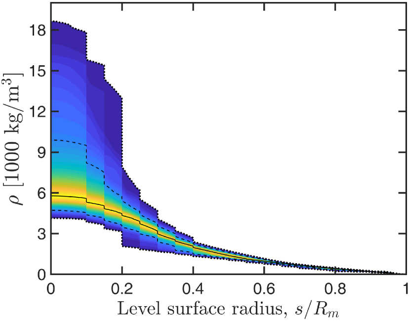
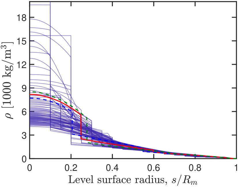
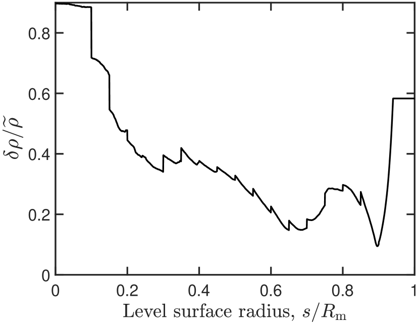
Two insights are possible by inspection of Figure 3. First, from the left panel, the observed gravity can constrain the top half of the planet much more strongly than it can the bottom half. This was expected (see Figure 1) but it is worth emphasizing again that it is a fundamental limitation of using gravity to probe the interior. This limitation is with us to stay; it will not be completely removed by increasing the accuracy of measurement or the precision of calculations. The same point is illustrated quantitatively in Figure 4 where the sample-spread of density values is shown for each radius.

Figure 4: Width of the distribution of density values found in the posterior sample at each radius. The quantity $\delta\rho$ is the difference of 84th and 16th percentile values, giving the equivalent of a 2-sigma spread; $\widetilde{\rho}$ is the sample-median density. The flat region near $s/R_{\text{m}}=1$ is a consequence of the relatively strong prior imposed in that region (see appendix C).

The second interesting feature, easier to spot in the right panel, is the existence of density discontinuities. Recall that our parameterization allowed up to two discontinuities; it did not require any. Indeed many profiles in the ensemble lack one or both discontinuities, the interpretation being that they lack a sharp composition or phase boundary.

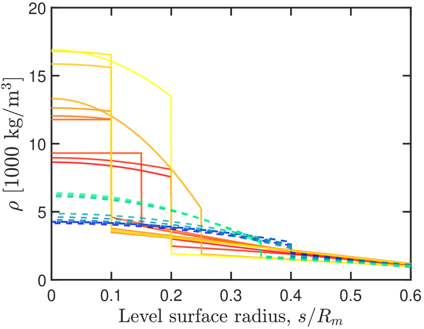
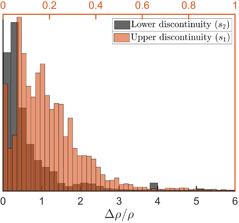
The inner discontinuity, at $s=s_{2}$, was meant to represent the possibility of a distinct core. Many density profiles indeed show a discontinuity pronounced enough to clearly indicate a transition to a heavy-element core, while in many others a much smaller density jump is observed instead, indicating a more subtle composition change, consistent perhaps with the idea of a fuzzy/dilute core (Helled & Stevenson, 2017) or compositional gradients (Leconte & Chabrier, 2012). For illustration, subsets from the sample with and without a pronounced discontinuity are shown in Fig. 5 (left panel). To put a probability value on the existence of a heavy-element core we can look at the distribution of $\Delta\rho/\rho$ at $s=s_{2}$, shown in Figure 6, but it is not clear what “cutoff” value should indicate the core/no-core property. For reference we can look at previously published, EOS-based models where a core was explicitly assumed. In such models the relative density jump at the core boundary exhibits a wide range, from as low as $\Delta\rho/\rho\approx{0.3}$ to more than tripling the density (e.g. Vazan et al., 2016; Mankovich et al., 2019, Mankovich et al. in review.). With this in mind perhaps the most precise statement to make is that at least half the density profiles in our sample show a discontinuity pronounced enough to be consistent with a heavy-element core transition.

The outer discontinuity, at $s=s_{1}$, was meant to represent the possibility of an abrupt change in density in the envelope, where the He mass fraction changes from depleted (relative to protosolar values) to enriched. This transition was expected based on theoretical considerations about the miscibility of He in H, in the region of phase space where hydrogen undergoes a molecular-to-metallic phase transition (Stevenson, 1975). An abrupt change in He mass fraction, $Y$, is often explicitly included in interior models, usually as a free parameter. However this two-layered envelope is only one possible arrangement among many, including a continuous $Y$ gradient. For example, if Saturn’s interior is sufficiently cold for He phase separation to occur in the first place then its true helium distribution is determined by the precise solubility of helium throughout the metallic interior, quantitative predictions of which have been made from first principles simulations (Schöttler & Redmer, 2018). Applying these predictions self-consistently to Saturn interior models, Mankovich & Fortney (2019) find equilibrium profiles wherein helium abundance increases continuously with depth inside $P\approx{2}\;\mathrm{Mbar}$ with the exception of a single deep discontinuous jump in density connecting the helium gradient region with a deeper pool of undissolved helium-rich material.

The sampled profiles include both continuous-density envelopes as well as those with small density jumps at $s_{1}$. While a density jump does not uniquely correspond to a jump in He abundance, a continuous $\rho(s)$ does imply continuous $Y(s)$. As seen in Figure 6, both possibilities (illustrated in the right panel of Fig. 5) are consistent with the observed gravity.

Figure 5: Left: A subset of profiles from the posterior distribution chosen to illustrate the idea of compact (solid lines) versus diluted (dashed lines) core. All have comparable likelihood values. A precise value of $\Delta\rho/\rho$ marking the difference between compact and diluted cores is hard to define (see discussion in text). Right: A subset of profiles from the posterior distribution chosen to illustrate the possibility of continuous He abundance in the envelope (solid lines) as well as the traditional idea of Helium rain separating He-poor and He-rich layers (dashed lines). Again, likelihood values of both subsets are comparable and, again, a precise cutoff below which the curve is considered continuous is not obvious.

Figure 6: Histograms of the density increase at the inner (bottom axis) and outer (top axis) discontinuities, perhaps representing a phase or composition change.

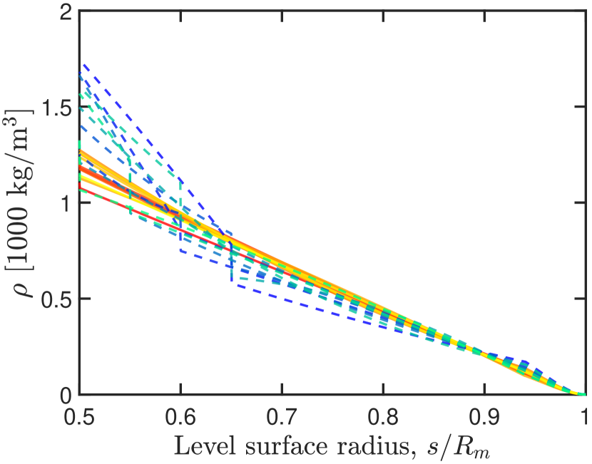
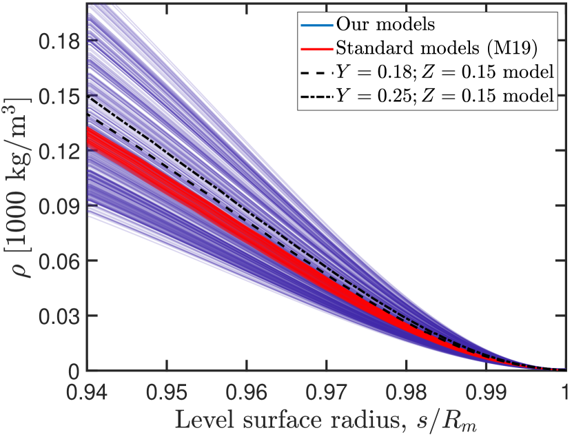
Perhaps the most useful aspect of the empirical-model approach is the possibility of finding unexpected solutions that can never arise where explicit composition modeling is used. Figure 7 takes a closer look at the density solutions, this time focusing on the low pressure region above $\sim\!\!{2\;\mathrm{GPa}}$. A long-standing point of tension in Saturn modeling is that Saturn’s atmosphere is known to be enriched in heavy elements (Atreya et al., 2016), showing about ten times the solar abundance for C, P, S (seen in CH₄, PH₃, and H₂S). That is, a “metals” mass fraction of $Z\approx{0.15}$ for the H/He envelope. However, modern Saturn models, even post Grand Finale, find a fit to the gravity field only with a much lower $Z<0.05$ in the outer H/He envelope (Iess et al., 2019; Mankovich et al., 2019; Nettelmann et al., 2013). Traditional models cannot match all of the atmospheric constraints, suggesting that we do not have a complete picture of Saturn’s interior. In contrast, we find that a natural outcome of our composition-agnostic approach is density-enhanced outer layers. For comparison we show two traditionally calculated models with $Z=0.15$ in their envelopes and they fall nicely inside our posterior sample. The density profiles in our sample (purple lines in Fig. 7) fit the measured gravity field while the traditional model cannot, with such high $Z$ fraction, because of quite different deeper interior profiles (Figure 3).

Figure 7: Density profiles in the upper envelope derived from our composition-agnostic sample (purple), traditional three-layer models with standard values of $Z\lesssim{0.05}$ (M19, red), and two three-layer models that have a much higher value of $Z=0.15$ consistent with atmospheric abundances (black dashed and dot-dashed) .

3.1 Inferences on possible composition

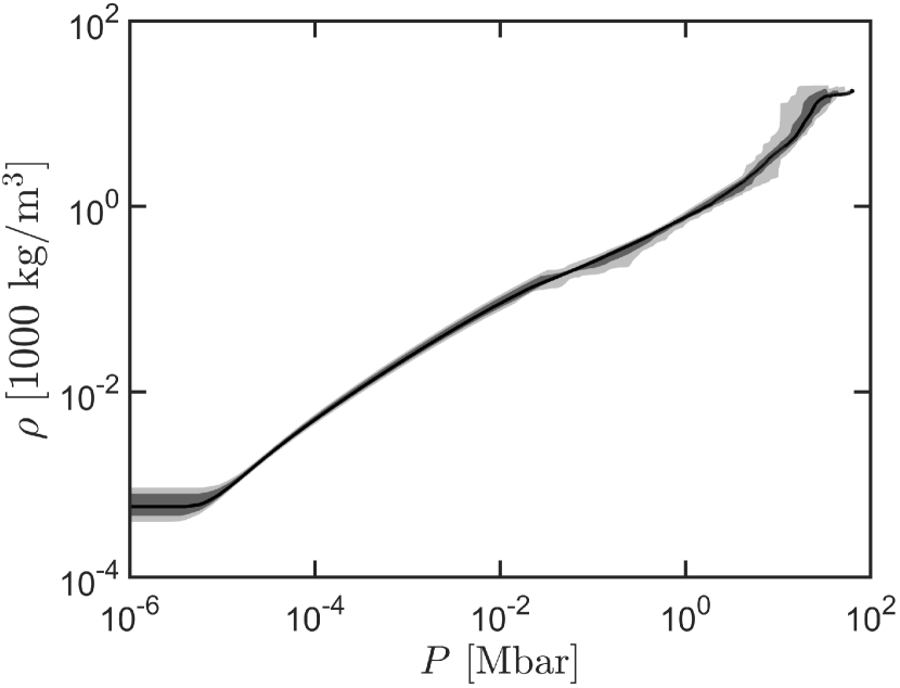
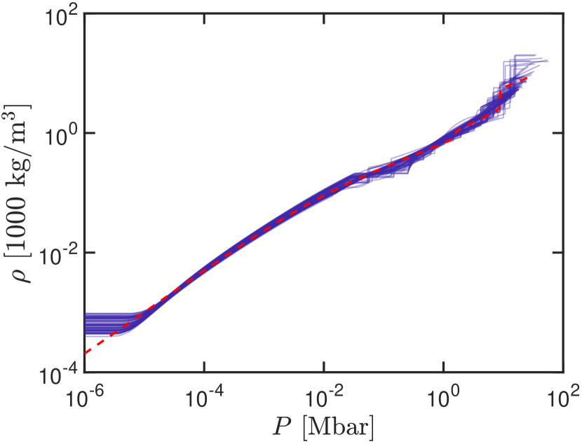
With each $\rho(s){}$ profile is associated a corresponding pressure profile, $P(s)$, by the assumption of hydrostatic equilibrium. Combining the two profiles to eliminate the radius variable results in a unique pressure-density relation, often called a barotrope. The posterior distribution of Saturn barotropes implied by our sample is shown in Figure 8. By itself the barotrope distribution does not provide much new insight, however it serves as the basis for the derivation of implied constraints on composition, by comparison with known equations of state, described next.

Figure 8: Visualization of the posterior distribution of empirical Saturn barotropes (pressure-density relations). Left: The sample median (thick black line), 16th to 84th percentile range (dark gray shaded), and 2nd to 98th percentile range (light gray shaded). Right: Thinned subset of sampled barotropes. The median barotrope implied by the physical models of M19 (red dashed line) overlaid for comparison.

So far we have focused our attention on what the gravity implies directly about the interior, avoiding additional assumptions. We now wish to see what can be inferred about the planet’s composition; some assumptions and approximations become necessary. The reason is that the density and pressure are not determined solely by composition; the thermal structure is a separate, and unknown, variable. Although the 1-bar temperature (to be used as a boundary condition) can be determined by observation, the interior thermal profile is unknown unless we make the strong and not entirely justified assumption of a single adiabatic profile extending at least some fraction of the way down into the planet (sec. 1.2).

A possible approach is to compare the empirical barotropes obtained above to some reference barotrope and examine the “residual” density for possible constraints on composition. Deviations of the density in the sampled profiles from this reference are due to a combination of the actual composition being different from the assumed reference and of the real temperature profile being different from adiabatic. This degeneracy means that we can only hope to estimate bounds on composition, rather than a nominal value.

In detail the calculation is this: Given the density $\rho$ and pressure $P$ on a level-surface with mean radius $s$ we can compute $\rho_{\text{bg}}=\rho_{\text{bg}}(P)$ using a background (bg) EOS and an assumed thermal gradient to compute a background barotrope. The residual density, $\rho-\rho_{\text{bg}}$, is already instructive, but we can further compute $\rho_{\text{fg}}=\rho_{\text{fg}}(P)$ using a foreground (fg) barotrope for heavy elements (water or rock) with the same pressure and temperature as the background. The heavy element mass fraction $Z$ then follows from the additive volume formula,

$$\frac{1}{\rho}=\frac{1-Z}{\rho_{\text{bg}}}+\frac{Z}{\rho_{\text{fg}}}.$$ (7)

The mass fraction $Z$, calculated with different choices for the foreground EOS, can be used to constrain the heavy element content consistent with the sampled density profiles.

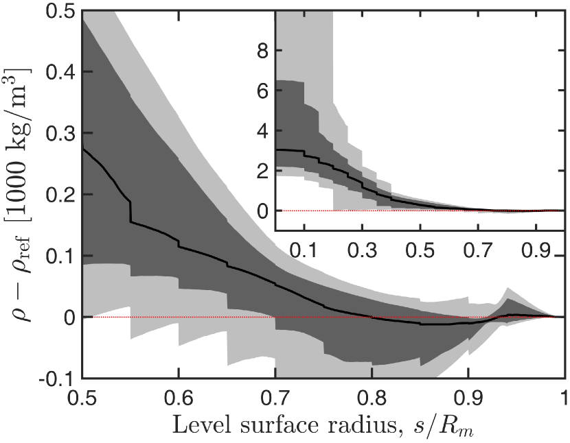
In the simplest case our background can be a mixture of only hydrogen and helium in protosolar mass fraction with an adiabatic temperature gradient. We use the EOS of Saumon et al. (1995) to generate pressure-density points for H ($X=0.725$ by mass) and He ($Y=0.275$ by mass) with constant entropy corresponding to a temperature $T=140\;\mathrm{K}$ at a pressure of $P=1\;\mathrm{bar}$. The residual density of the sampled profiles relative to this background is shown in Fig. 9. Clearly, there is an excess density compared to the adiabat in the regions of the planet below $70\%$ of the planet’s radius, which becomes extreme in the inner $30\%$. If a lower $Y$ reference adiabat were chosen in the outer layers, larger density excess would be needed.

Figure 9: Residual density above a background derived from a reference adiabat calculated for a H/He mixture with He mass fraction $Y=0.275$ and $T(1\;\mathrm{bar})=140\;\mathrm{K}$. The thick curve is the sample median and the dark and light shaded regions include 68% and 96% of the sample, respectively.

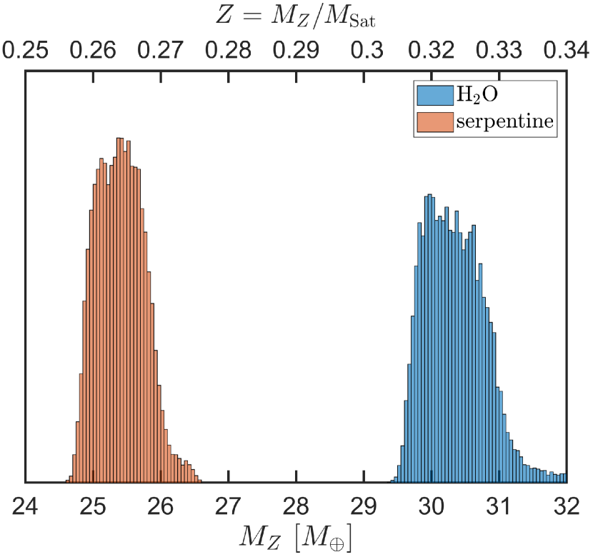
Next, using a foreground EOS for either pure water ice (French et al., 2009; Thompson, 1990) or pure rock (Thompson, 1990) we apply eq. (7) to each of the sampled profiles. What we obtain is an empirical probability distribution of the heavy element content in Saturn’s interior. In Figure 10 we plot a histogram of this distribution, which should be taken as an estimated upper bound rather than a precise distribution, given the assumptions underlying this calculation. These values are typically higher than those from standard models because the excess heavy elements, even at high pressure where one might expect a pure-heavy-element core, are here always determined as an excess density over that of the lower density H/He.

Figure 10: Residual mass in heavy elements and corresponding residual bulk metallicity assuming either pure H₂O ice or pure serpentine rock EOS. These are end members of what is likely a mixture of both materials in unknown ratio. The figure shows the mass in heavy elements inferred with a reference density based on a H/He adiabat with $Y=0.275$ extending throughout the planet, and should be interpreted as an upper bound since it excludes the possibility of a pure heavy-element core.

Figure 11: Same as Fig. 9 but background density derived from adiabat calculated for $Y=0.1$ and $Z=0.135$.

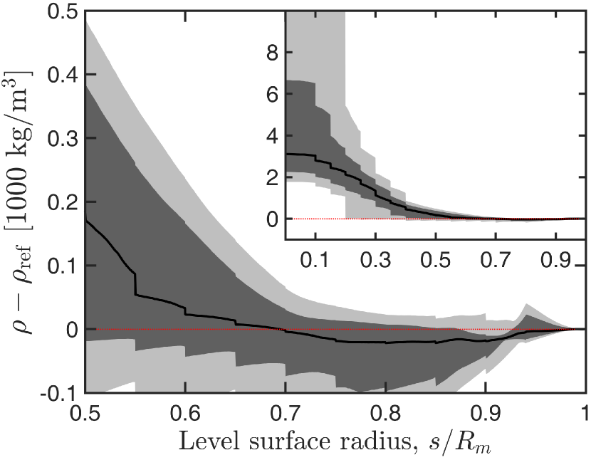
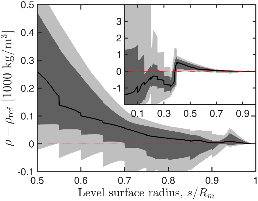
As a last example we use as our reference background the end state of a recent Saturn thermal evolution model (Mankovich & Fortney, 2019). This structure derives from calculation of the cooling of Saturn’s interior, including the phase separation of He from H in the interior. This leaves the molecular part of Saturn’s The model matches Saturn’s present-day radius and intrinsic luminosity but does not attempt to match the observed gravity field. Subtracting this background density we again examine the residual density in the sampled profiles (Figure 12). These observations are at the 1–2$\sigma$ level, i.e., solutions also exist that do not follow these trends.

Figure 12: Same as figure 9 but with the background density defined by the end state of an evolution model (Mankovich & Fortney, 2019).

4 Discussion and Conclusions

In this paper we presented an empirical approach to using gravity data to explore the interior structures of fluid planets and applied it to Saturn using data from Cassini’s Grand Finale orbits. Here we wish to summarize our findings for Saturn, and about planetary interior modeling in general, and to consider the strengths and weaknesses of our “density first” approach, versus traditional, composition-based modeling.

First, a point that was already made above but bears repeating: Gravity data alone offers robust but loose constraints. The great variety of density profiles included in our sample may seem surprising and counter-intuitive but it is an unavoidable consequence of using an integrated quantity, in this case the external potential, to study the spatial distribution of local quantities, in this case, the interior density and all properties of the planet that derive from it. Without imposing additional constraints we necessarily obtain non-unique solutions, and this is a separate and more fundamental limitation than the problem of uncertainty in the data and/or calculation.

As a result, the main finding we can report on, with respect to Saturn, is to confirm the well-known but often underappreciated suspicion that solutions to Saturn’s gravitational potential field exist that do not conform to a simple model of a few compositionally homogeneous and thermally adiabatic layers. While this may not be a surprise, it is nevertheless a previously unproven result. We could not know, a priori, whether the non-uniqueness of gravity solutions would translate to a narrow range of allowed interior structures or to a wide variety, as appears to be the case.

We can contrast this with the seemingly more informative but less robust outcomes from traditional models. These are often able to report narrow ranges for a number of key quantities (typically core mass, bulk metallicity, H/He envelope metallicity, atmospheric helium depletion) that were the free parameters in the chosen model. The trade off for these precise, straightforward estimates is their unknown validity, being tied to very particular and often very simple a priori modeling framework for the planet. Conversely, the results we report on here are of much wider validity, with the trade off of being much less specific and more difficult to interpret.

Finally, our inferred heavy-element mass for Saturn relied on the SCVH EOS for H-He. This widely-used EOS has been recently updated to be more thermodynamically consistent (Chabrier et al., 2019). In the updated version, hydrogen is found to be denser under Jupiter and Saturn conditions, in agreement with DFT calculations. Therefore the heavy-element masses listed here are likely to represent upper bounds. Clearly, a more detailed investigation of that topic in the future is desirable.

4.1 Narrowing down the posterior distribution

It is certainly possible that a subset of the sampled density profiles can be “disqualified” based on other physical considerations, and indeed we consider this a natural avenue for future work. Any reduction of the allowed solution space will be an improvement, as it narrows down the probable actual structure of Saturn. However any such reductions must be considered carefully, so that they do not rely too strongly on implicit assumptions of the exact kind we decided to avoid in the first place. Such low-hanging fruit as disqualifying unphysical density inversions or density extremes had already been picked by passing an appropriate prior probability function, $p(\mathbf{x})$, to the MCMC sampler (appendix C). For instance, that is why the posterior sample does not contain profiles with stationary points or with central densities much higher than ${2}\times{}10^{4}\;\mathrm{kg/m^{3}}$. More subtle constraints, e.g., looking for convective instabilities or checking pressure-density pairs against known equations-of-state, require knowledge of the thermal state and inevitably require additional assumptions.

A second and unrelated way to narrow the predicted distribution somewhat is to “sharpen” the likelihood function by including higher order coefficients and/or with tighter uncertainties. Recall that $J_{2}$ and $J_{4}$ are known for Saturn with better accuracy than was assumed in eq. (4). The same is true for Jupiter, and higher-order coefficients are also known, with decreasing accuracy, for both planets. More precise calculation of the Js for a given density profile can reach this level of accuracy, with the only down side being increased computation time.

What we have accomplished is an understanding of a much fuller range of interior density profiles for Saturn that are allowed by the planet’s gravity field as determined by the Cassini Grand Finale, a data set that will likely not be surpassed for some decades. We hope that the allowed density distributions are a long-lived data product that other workers may find useful as new ideas about planetary formation, structure, and evolution emerge. Such ideas can be compared against the allowed interior density distributions that we have found here. To facilitate this we archive the data products and analysis tools used in this study, documented in sufficient detail to allow reuse and alternative analysis. The archive can be found at https://doi.org/10.7291/D1P07G.

Appendix A A single-parameter description of low pressure region

As explained in sec. 2.2, when choosing a parameterization our goal is to find the best compromise between a simple description, with a small number of parameters suitable for MCMC sampling, and a general description, letting the resulting $\rho(s){}$ curves explore all reasonable profiles. Our choice of parameterization by piecewise-quadratic functions was guided by, but much more general than, previously published models that were based on physical EOSs and an adiabatic temperature gradient (Mankovich et al., 2019). We found that, for the bulk of the planet, a piecewise-quadratic $\rho(s){}$ is able to capture the profiles derived with a physical EOS and flexibly explore beyond them.

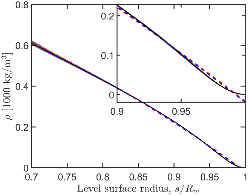
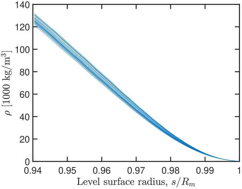
However, empirical $\rho(s){}$ profiles derived from this parameterization inevitably exhibit a small but significant deviation from profiles derived by physical models, in a small region at the top of the upper envelope. Figure 13 illustrates the problem. An inflection is seen in all the EOS-based $\rho(s)$ curves, always in the neighborhood of $s/R_{m}\approx{0.95}$, and this inflection cannot be captured if a single polynomial is used to approximate the entire upper envelope (typically extending down to at least $s/R_{m}\approx{0.65}$). Above the inflection point is a small region where $\rho(s)$ seems to follow a different curve. And yet this small region of the upper envelope is one where physical models are most reliable, at a pressure and temperature region where equations of state are well tested and where an adiabatic temperature gradient is expected to exist. Closely matching the EOS-based models in this upper region of the planet is an important way by which to constrain empirical models.

The obvious solution is to add an additional segment to the piecewise-polynomial parameterization but unfortunately this cannot be implemented. The problem is not simply that this would require 5-6 additional parameters and greatly complicate the sampling process. More seriously, the small region in question contains relatively little mass. Small changes in density in this region do not make a big enough difference in the $J$ values, at our level of precision, to effectively “drive” the likelihood function. There is no reason to expect then that profiles from the resulting posterior would be any more like the EOS-based ones.

Instead, we use a more explicit constraint, ad-hoc in nature, which achieves the desired result of keeping the top of the envelope in empirical models similar to EOS-based models while retaining enough flexibility to mimic varying composition.

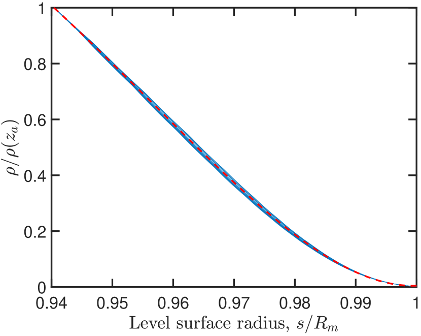
We examine the shapes of the density profiles of M19 in the region above $z_{a}=s/R_{m}=0.94$ (fig. 14a). We choose this fixed point, slightly below the inflection seen in the models, to make sure we always capture the slope accurately. For $z<z_{a}$ we use the main parameterization by piecewise-quadratics (eq. (3) and appendix B). Above $z_{a}$, we find that all profiles can be fit by fourth-degree polynomials (quartics) to excellent agreement. Further, if we denote $\rho_{a}=\rho(z_{a})$ we find that, for $z_{a}\leq{z}\leq{1}$, the curves $\rho(z)/\rho_{a}$ are equally well fit by quartics (not surprising), and in fact that they can all be adequately approximated by the same quartic polynomial:

$$\frac{\rho(z_{a}\leq{z}\leq{1})}{\rho(z_{a})}\approx Q(z)=(3\times{10}^{4})z^{4}-(1.128\times{10}^{5})z^{3}+(1.587\times{10}^{5})z^{2}-(9.914\times{10}^{4})z+(2.323\times{10}^{4}),$$ (A1)

shown in fig. 14b. The profiles in fig 14a can be recovered, approximately but with high fidelity, by multiplying the polynomial (A1) by a particular value of $\rho_{a}$.

In other words, in the region $z\geq{z_{a}}$ the physical, EOS-based models form a one-parameter family of quartic functions. We do not see special physical meaning here. It is simply that the variation in density that originated from making different choices about composition (i.e., the envelope’s helium mass fraction and metallicity) under the severe but, in this region, well-justified adiabatic assumption, can be empirically captured by varying the value of $\rho_{a}=\rho(s/R_{m}=0.94)$. To make sure that our empirical profiles are similar to but not overly constrained by EOS-based models in the region $z\geq{z_{a}}$ all we have to do is set an appropriate prior on the parameter $\rho_{a}$. Guided again by the physical models we choose a uniform prior in the range $100\;\mathrm{kg/m^{3}}\leq{\rho_{a}}\leq{200}\;\mathrm{kg/m^{3}}$ with an exponentially decaying probability outside this range.

Figure 13: A close look at the upper envelope of traditional Saturn models (Mankovich et al., 2019), the same models seen in fig. 2 in the main text. The solid black curve is the ensemble median density at each radius, with the light gray band denoting the 1-$\sigma$ variation. The red and blue dashed lines are best-fit polynomials of degree 2 and 4 approximating the density profile in the upper envelope as a whole. Neither is a good approximation in the small region where $s\gtrsim{0.95}R_{m}$.

Figure 14: The same profiles as in fig. 13 truncated at $s/R_{m}=0.94$, slightly below the inflection point. The apparently similar curvature motivates us to fit them all with a single quartic polynomial in $z=s/R_{m}$ by normalizing to the value $\rho_{a}=\rho(z_{a}=0.94)$. This polynomial, eq. (A1), together with a posterior distribution of $\rho_{a}$ generate density profiles that resemble the physical models in shape but are free to explore “around” them.

Appendix B Complete definition of parameters sampled by MCMC

As explained in sec. 2.2 of the main text, our choice of parametrization of empirical density profile is a piecewise quadratic function. There are two breakpoints, at normalized radii $z_{1}$ and $z_{2}$, where a jump discontinuity is explicitly allowed (but not required) and between them are three quadratic segments each defined by three parameters, for a total of 11 free parameters required to define a density profile $\rho(s){}$.

There is more than one way to let three numbers define a quadratic function. In principle all are equivalent but in practice MCMC sampling works best (i.e. converges fastest) when the parameters are minimally correlated and the likelihood function is a smooth function of their numerical values. It is especially important to avoid likelihood “cliffs”, where a small change in one parameter value results in a sudden drop in the likelihood value, perhaps because a physically motivated prior condition has been violated. This is a real danger and often leads the most intuitive and simple parametrizations to fail.

For example, defining the quadratic segments by

$$\rho(z)=\begin{cases}a_{1}z^{2}+b_{1}z+c_{1},&z_{1}<z,\\ a_{2}z^{2}+b_{2}z+c_{2},&z_{2}<z\leq z_{1},\\ a_{3}z^{2}+b_{3}z+c_{3},&z\leq z_{2},\end{cases}$$ (B1)

would not do. The 9 parameters $a_{i},b_{i},c_{i}$ are highly correlated, meaning a small change in the value of one usually requires a simultaneous and “coordinated” change in several others to prevent the resulting density profile from changing too much and landing in a low-likelihood region. Worse, the locus of parameter values that yield physically permissible density profiles (without negative density or any density inversions) form distinct islands in parameter space, with zero-likelihood regions between then that are practically impossible for MCMC algorithms to cross.

By trial and error we arrive at the following alternative parameterization; admittedly complicated, but effective. In addition to $z_{1}$ and $z_{2}$, the 9 parameters defining the quadratic segments are:

$$\begin{split}\mathbf{x}=\bigl{[}&a_{1},\ \rho_{10},\ y_{11}=\log(\rho_{11}-\rho_{10}),\\ &a_{2},\ y_{21}=\log(\rho_{21}-\rho_{11}),\ y_{22}=\log(\rho_{22}-\rho_{21}),\\ &a_{3},\ y_{32}=\log(\rho_{32}-\rho_{22}),\ y_{33}=\log(\rho_{33}-\rho_{32})\bigr{]}.\end{split}$$ (B2)

The parameters $a_{i}$ control the curvature of segment $i$ and the $\rho_{ij}$ are the densities at the segment ends. The segments are numbered from top to bottom: segment 1 includes $z_{1}<z\leq{z_{a}=0.94}$, segment 2 includes $z_{2}<z\leq{z_{1}}$, and segment 3 includes $0<z\leq{z_{2}}$. (See appendix A for why the top segment extends up to $z_{a}$ instead of $z=1$.)

Next, $\rho_{10}=\rho(z_{a})$ (top of segment 1) and $\rho_{11}=\lim_{z\to{}z_{1}^{+}}\rho(z)$ is the right-limit density at $z_{1}$ (i.e. bottom of segment 1). Similarly, $\rho_{21}=\lim_{z\to{}z_{1}^{-}}\rho(z)$ is the left-limit density at $z_{1}$ (top of segment 2) and $\rho_{22}=\lim_{z\to{}z_{2}^{+}}\rho(z)$ is the right-limit density at $z_{2}$ (bottom of segment 2). Finally, $\rho_{32}=\lim_{z\to{}z_{2}^{-}}\rho(z)$ is the left-limit density at $z_{2}$ (top of segment 2) and $\rho_{33}=\rho(z=0)$ is the density at the bottom of segment 3, the center of the planet.

The use of curvature-and-endpoints description is less familiar but more intuitive than the well known polynomial coefficients representation. Notice that the endpoint density values are defined implicitly, the actual parameter values are the log of difference of neighboring density values. This transformation is a common MCMC “trick.” It allows the sampled parameters to have values in the range $[-\infty,\infty]$ and keeps the corresponding physical parameters in their meaningful range. All values of $y_{ij}$ are permissible and lead to physical, monotonically decreasing density profiles. Larger values of $y_{21}$ and $y_{32}$ lead to more pronounced density jumps between segments, while more negative values result in the jumps disappearing and the segments merging into one. Thus all possibilities from the canonical, sharp envelope-envelope and core-envelope transitions to a completely smooth density profile throughout are representable and reachable by continuous variation of parameter values.

The density profile itself is constructed from the parameters by solving for the polynomial coefficients that reproduce the end-point densities:

$$\rho(z)=\begin{cases}a_{1}(z^{2}-z_{a}^{2})+\bigl{[}\frac{\rho_{11}-\rho_{10}}{z_{1}-z_{a}}-a_{1}(z_{1}+z_{a})\bigr{]}(z-z_{a})+\rho_{10},&z_{1}<z\leq{z_{a}},\\ a_{2}(z^{2}-z_{1}^{2})+\bigl{[}\frac{\rho_{22}-\rho_{21}}{z_{2}-z_{1}}-a_{2}(z_{2}+z_{1})\bigr{]}(z-z_{1})+\rho_{21},&z_{2}<z\leq{z_{1}},\\ a_{3}(z^{2}-z_{2}^{2})+\bigl{[}\frac{\rho_{33}-\rho_{32}}{0-z_{2}}-\,a_{3}(0+z_{2})\;\bigr{]}(z-z_{2})+\rho_{32},&\;0<z\leq{z_{2}}.\end{cases}$$ (B3)

The prior probabilities set for the above parameters and the resulting posterior chains are given in appendix C.

Appendix C Sampling procedure

The full list of parameters we need to explore is:

$$\mathbf{x}=\{m_{\text{rot}},a_{1},y_{10},y_{11},a_{2},y_{21},y_{22},y_{32},y_{33},z_{1},z_{2}\}.$$ (C1)

See appendix B for the meaning of these parameters. Notice that $a_{3}$ is apparently missing from the list above. In fact, as explained in sec. 2.5, the requirement that $\lim_{s\to{0^{+}}}d\rho(s)/ds=0$ constrains the innermost segment of $\rho(s)$ such that only two parameters are independent. The curvature of that segment follows:

$$\begin{split}\rho_{10}&=y_{10},\\ \rho_{11}&=\rho_{10}+\exp(y_{11}),\\ \rho_{21}&=\rho_{11}+\exp(y_{21}),\\ \rho_{22}&=\rho_{21}+\exp(y_{22}),\\ \rho_{32}&=\rho_{22}+\exp(y_{32}),\\ \rho_{33}&=\rho_{32}+\exp(y_{33}),\\ a_{3}&=\frac{(\rho_{32}-\rho_{33})}{z_{2}^{2}}.\end{split}$$ (C2)

In sec. 2.5 we explain that the high degree of correlation between the variables in (C1) makes it very difficult to sample from the full posterior simultaneously. We find it necessary to sample instead from the conditional probabilities, $p_{\mathbf{z}}=p(\mathbf{x^{\prime}}|\mathbf{Z=z})$, where $\mathbf{Z}=\{z_{1},z_{2}\}$ and $\mathbf{x^{\prime}}=\mathbf{x}\setminus{\mathbf{Z}}$. In words: we fix values for the radii $z_{1}$ and $z_{2}$ and sample the remaining 10 parameters, resulting in a conditional distribution. We repeat this for many values of $z_{i}$ to build a picture of the full posterior.

C.1 Prior probabilities of sampled parameters

The prior for $\mathbf{x}$ is a product of independent priors for each component. The rotation prior is $m_{\text{rot}}\sim\mathcal{N}\,(0.14224,4.5\times{10^{-4}})$. The mean corresponds to a rotation period of 10h:33min:30s and the deviation is about 1 minute.

The curvature parameters take a uniform prior $a_{i}\sim\mathcal{U}\,(-3\times{10^{6}},3\times{10^{6}})$. These limits do not have a special physical meaning, they are reasonable bounds we find by experimentation.

The parameter $y_{10}=\rho_{a}$ has a particularly important prior. Recall that this is a density at a reference point $\rho_{a}=\rho(z_{a}=0.94)$ that we use to keep the density in the low-pressure region of the envelope compatible with values derived in traditional, EOS-based models. Guided by the models presented in (Mankovich et al., 2019) we set

$$\log{p(y_{10})}\sim-\frac{1}{2}\left(\frac{100-\min(y_{10},100)}{10}+\frac{\max(y_{10},200)-200}{10}\right)^{2},$$ (C3)

and the numerical values are in $\mathrm{kg}/\mathrm{m}^{3}$. In words: it is a uniform probability inside the 100 to 200 $\;\mathrm{kg/m^{3}}$ range with exponentially decaying probability outside of it with an e-folding distance of $10\;\mathrm{kg/m^{3}}$.

The other $y_{ij}$ parameters are logarithms of density differences. They can take positive or negative values, and the values get exponentiated and added to define the densities at the end points of the quadratic segments, $\rho_{ij}$. It is natural to define the prior on the actual density values, say a uniform prior in the 0 to 30,000 $\;\mathrm{kg/m^{3}}$ range (merely a guess as to the highest density achievable in Saturn). We need to be careful though. The transformation from $\rho_{ij}$ to $y_{ij}$ involves a transformation of the probability; the prior on $y_{ij}$ is not uniform. Instead it follows from conservation of probability mass in equivalent parts of the distribution: $p_{\rho}(\rho^{\prime})\,d\rho^{\prime}=p_{y}(y^{\prime})\,dy^{\prime}$. The answer is $y_{ij}\sim{}e^{y^{\prime}}\mathcal{U}(-\infty,\infty)$, but it helps to cut off the uniform probability outside of a reasonable range. The final prior therefore is

$$\log{p(y_{ij})}\sim\begin{cases}y_{ij}&-20<y_{ij}<12,\\ -\infty&\text{otherwise}.\end{cases}$$ (C4)

There is no prior on $z_{1}$ and $z_{2}$ because they are not MCMC sampled.

C.2 Sampling from the conditional distributions

We obtain a sample from $p_{\mathbf{z}}$ for each pair $\{z_{1},z_{2}\}\in\{0.35,0.4,0.45,\ldots,0.9\}\times\{0.1,0.15,0.2,\ldots,0.4\}$ subject to the condition $z_{1}>z_{2}$. There are 81 pairs and thus 81 separate MCMC runs to produce samples from the different conditional distributions. We use the implementation of ensemble sampling in emcee, with the default stretch move algorithm, and run 78 walkers for 60000 steps each.

Trace plots for one such MCMC run are shown in Figure 15, similar behavior is exhibited in all runs. Visual inspection of trace plots is one method of deciding what part of the MCMC chain we can use to take independent samples from. Inspection of figure 15 reveals why we had to use many walkers for so many steps. Several of the parameters exhibit slow mixing, taking more than 30000 steps to fully forget their seed state. Even worse than the long burn-in time is the low acceptance rate, which leads to quite long autocorrelation in many dimensions. In other words, successive steps are not independent, requiring about 200 steps to become uncorrelated. This means that an MCMC run evaluating more than 4.5 million candidate models produces only about 10,000 usable ones.

Figure 15: Trace plots from MCMC run with $z_{1}=0.65$ and $z_{2}=0.2$.

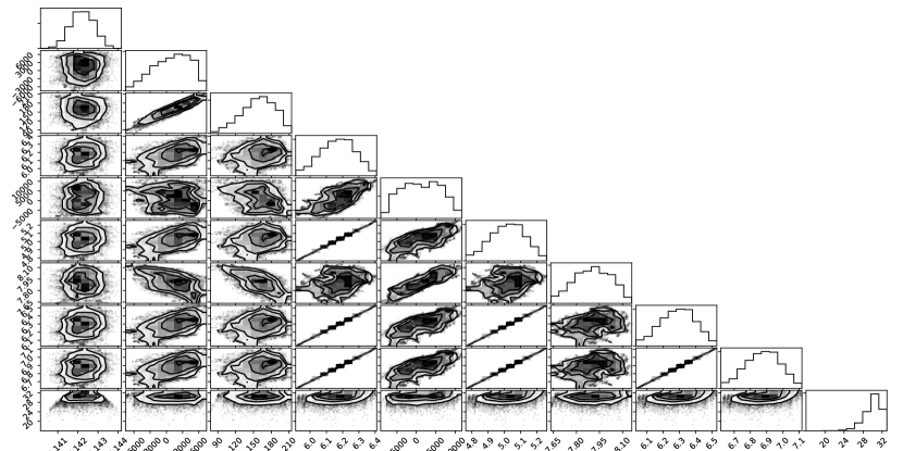
It is common practice to display the results of MCMC sampling in a series of series of two-dimensional histograms of parameter pairs. This visualization, often called a corner plot, is a convenient way to quickly make sense of the distribution of parameters including the relationships between them. In our case the parameters are too far removed from a physical meaning for us to derive any useful insight from their pair-wise histograms. We include the corner plot for one MCMC run anyway, in Figure

Figure 16: Corner plot of parameters sampled for the $z_{1}=0.65$ $z_{2}=0.2$ conditional probability (same run as Fig. 15), after discarding the first 30,000 steps from each walker and thinning the rest by keeping one in every 200 steps. The subplot in the $i$-th row and $j$-th column is the two-dimensional histogram of parameters $i$ and $j$, as ordered in eq. (C1).

C.3 Combining the conditional probabilities into a single posterior.

After culling the MCMC chains we have what we hope are independent samples from the conditional probabilities $p_{\mathbf{z}}$. Next we need to combine subsets from these samples in a way that approximates a sample from the full posterior, $p(\mathbf{x})$. This task is similar to the model selection problem of Bayesian inference. We have found parameter distributions for different statistical models, and we wish to use this information to evaluate the relative likelihood between the models, in our case between interior profiles with different locations of discontinuous density. If we know the relative likelihoods we can combine subsets from the individual models in proportion to their likelihood to obtain our posterior sample.

Although this is a common and well studied task it is nevertheless a difficult one, and there is no known best method or even useful error bounds. Nelson et al. (2018) report on a thorough comparison of many different approaches to this problem (often referred to as calculating the posterior odds or the Bayes factor or the evidence integral or simple the evidence), including the method we chose which is based on calculating the Bayes Information Criterion, or BIC:

$$\mathrm{BIC}(\mathbf{z})=-2\log(max_{\mathbf{x}}(p_{\mathbf{z}}(\mathbf{x^{\prime}})))+\log{N},$$ (C5)

where $k$ is the number of model parameters and $N$ is the number of data points. The relative likelihood is given by

$$\frac{p_{\mathbf{z_{a}}}}{p_{\mathbf{z_{b}}}}=\exp(-(\mathrm{BIC}_{\mathbf{z_{b}}}-\mathrm{BIC}_{\mathbf{z_{a}}})/2).$$ (C6)

In our case, $k=9$ always and $N\approx{10^{4}}$, and the maximum likelihood is likewise very similar between all 81 conditional samples. So it happens that the pairwise relative likelihood among all the conditional distributions is close to one. We take random draws from the 81 conditional samples, in almost equal proportions, to obtain a single set of 20,000 hopefully independent draws from the unknown posterior, $p(\mathbf{x}|\mathbf{OBS})$. Histograms of the 12 parameters (including $a_{3}$ which is not sampled but uniquely determined by eq (C2)) are shown in Figure 17. These are the parameters used to reconstruct the density profiles shown in Figure 3 and to perform the analysis in the rest of the paper.

Figure 17: Histograms of parameter values used to construct the density profiles used in this work.

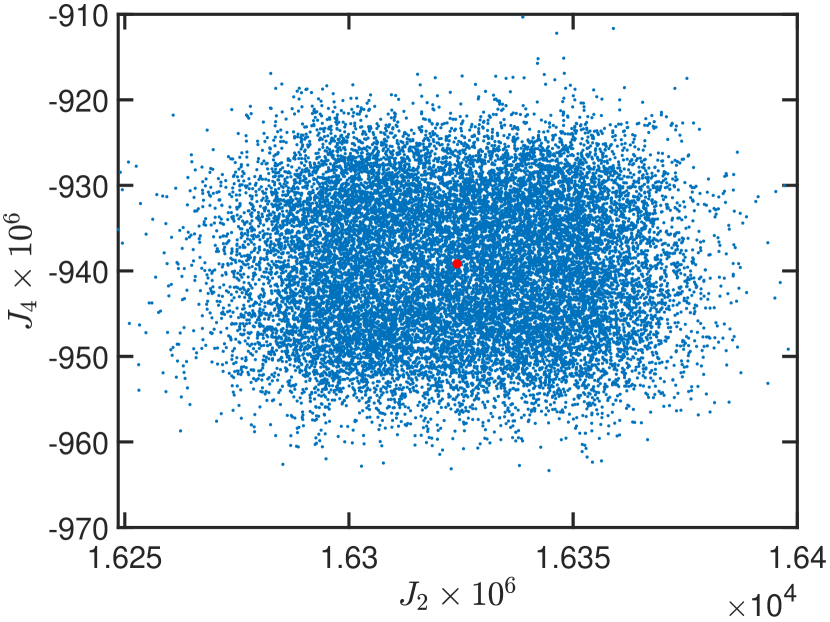
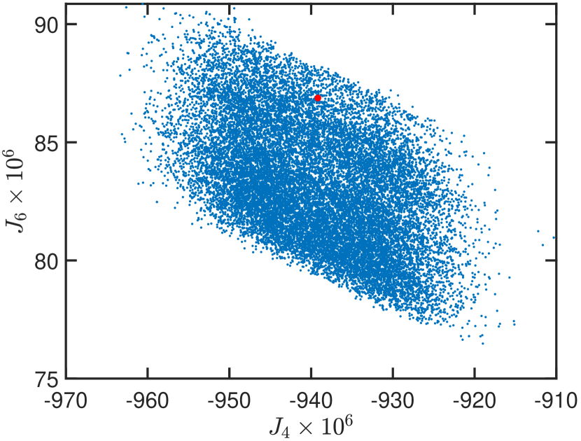
Finally, the distribution of empirical models from our sample in the $J_{2}\text{-}J_{4}$ and $J_{4}\text{-}J_{6}$ planes is shown in Figure 18. In many previous works that use the gravity field to study the planetary interior this is a central result and a similar plot would be a prominent figure in the main text. In the traditional modeling approach this is a useful indication of how variation of model parameters (which in traditional models have important physical meaning) translates to variation in the model’s gravity. In our empirical, MCMC-driven study however this distribution is much less informative. Recall that the sampling algorithm is driven by a likelihood function that compares model values of $J_{i}$ with observed values. Unless there is a bug in the implementation, the $J_{i}$ distribution in the final sample is determined entirely by the choice of likelihood function and tells us nothing about the underlying model. Nonetheless, we include this figure to potentially help a direct comparison with past or future investigations.

Figure 18: Gravitational harmonics of the empirical models of Fig. 3 of the main text. The coefficients for Saturn’s observed gravity (Iess et al., 2019) are indicated by a red circle.

References

- Atreya et al. (2016) Atreya, S. K., Crida, A., Guillot, T., et al. 2016, ArXiv e-prints 1606.04510. https://arxiv.org/abs/1606.04510
- Chabrier et al. (2019) Chabrier, G., Mazevet, S., & Soubiran, F. 2019, Astrophys. J., 872, 51, doi: 10.3847/1538-4357/aaf99f
- Cowles & Carlin (1996) Cowles, M. K., & Carlin, B. P. 1996, J. Am. Stat. Assoc., 91, 883
- Debras & Chabrier (2019) Debras, F., & Chabrier, G. 2019, Astrophys. J., 872, 100, doi: 10.3847/1538-4357/aaff65
- Desch & Kaiser (1981) Desch, M. D., & Kaiser, M. L. 1981, Geophys. Res. Lett., 8, 253, doi: 10.1029/GL008i003p00253
- Foreman-Mackey et al. (2013) Foreman-Mackey, D., Hogg, D. W., Lang, D., & Goodman, J. 2013, Publ. Astron. Soc. Pacific, 125, 306, doi: 10.1086/670067
- Fortney et al. (2018) Fortney, J. J., Helled, R., Nettelmann, N., et al. 2018, in Saturn 21st Century, ed. K. H. Baines, M. F. Flasar, N. Krupp, & T. Stallard (Cambridge University Press), 44–68
- Fortney & Hubbard (2003) Fortney, J. J., & Hubbard, W. B. 2003, Icarus, 164, 228, doi: 10.1016/S0019-1035(03)00130-1
- French et al. (2009) French, M., Mattsson, T. R., Nettelmann, N., & Redmer, R. 2009, Phys. Rev. B, 79, 54107, doi: 10.1103/PhysRevB.79.054107
- Galanti & Kaspi (2017) Galanti, E., & Kaspi, Y. 2017, Astrophys. J., 843, L25, doi: 10.3847/2041-8213/aa7aec
- Galanti et al. (2019) Galanti, E., Kaspi, Y., Miguel, Y., et al. 2019, Geophys. Res. Lett., 616, doi: 10.1029/2018GL078087
- Goodman & Weare (2010) Goodman, J., & Weare, J. 2010, Commun. Appl. Math. Comput. Sci., 5, 65
- Guillot et al. (2018) Guillot, T., Miguel, Y., Militzer, B., et al. 2018, Nature, 555, 227, doi: 10.1038/nature25775
- Helled (2011) Helled, R. 2011, Astrophys. J. Lett., 735, doi: 10.1088/2041-8205/735/1/L16
- Helled et al. (2011a) Helled, R., Anderson, J. D., Podolak, M., & Schubert, G. 2011a, Astrophys. J., 726, doi: 10.1088/0004-637X/726/1/15
- Helled et al. (2011b) Helled, R., Anderson, J. D., Schubert, G., & Stevenson, D. J. 2011b, Icarus, 216, 440, doi: 10.1016/j.icarus.2011.09.016
- Helled et al. (2015) Helled, R., Galanti, E., & Kaspi, Y. 2015, Nature, doi: 10.1038/nature14278
- Helled & Guillot (2013) Helled, R., & Guillot, T. 2013, Astrophys. J., 767, doi: 10.1088/0004-637X/767/2/113
- Helled et al. (2009) Helled, R., Schubert, G., & Anderson, J. D. 2009, Icarus, 199, 368, doi: 10.1016/j.icarus.2008.10.005
- Helled & Stevenson (2017) Helled, R., & Stevenson, D. J. 2017, Astrophys. J. Lett., 840, L4, doi: 10.3847/2041-8213/aa6d08
- Hubbard (2013) Hubbard, B. 2013, Astrophys. J., 768, 43
- Hubbard (2012) Hubbard, W. 2012, Astrophys. J. Lett., 756, L15, doi: 10.1088/0004-637X/768/1/43
- Hubbard (1982) Hubbard, W. B. 1982, Icarus, 52, 509, doi: 10.1016/0019-1035(82)90011-2
- Hubbard et al. (1995) Hubbard, W. B., Podolak, M., & Stevenson, D. J. 1995, in Neptune Trit., ed. D. P. Cruikshank, M. S. Matthews, & A. M. Schumann, 109–138
- Iess et al. (2019) Iess, L., Militzer, B., Kaspi, Y., et al. 2019, Science (80-. )., 2965, eaat2965, doi: 10.1126/science.aat2965
- Jacobson et al. (2006) Jacobson, R. A., Antreasian, P. G., Bordi, J. J., et al. 2006, Astron. J., 132, 2520, doi: 10.1086/508812
- Kaspi et al. (2018) Kaspi, Y., Galanti, E., Iess, L., & Durante, D. 2018, in AAS/Division for Planetary Sciences Meeting Abstracts, Vol. 50, AAS/Division Planet. Sci. Meet. Abstr., 500.07
- Kaspi et al. (2013) Kaspi, Y., Showman, A. P., Hubbard, W. B., Aharonson, O., & Helled, R. 2013, Nature, 497, 344, doi: 10.1038/nature12131
- Leconte & Chabrier (2012) Leconte, J., & Chabrier, G. 2012, Astron. Astrophys., 20, 1, doi: 10.1051/0004-6361/201117595
- Ledoux (1947) Ledoux, P. 1947, Astrophys. J., 105, 305, doi: 10.1086/144905
- Lindal et al. (1985) Lindal, G. F., Sweetnam, D. N., & Eshleman, V. R. 1985, Astron. J., 90, 1136, doi: 10.1086/113820
- Mankovich et al. (2016) Mankovich, C., Fortney, J. J., & Moore, K. L. 2016, Astrophys. J., 832, 1, doi: 10.3847/0004-637X/832/2/113
- Mankovich et al. (2019) Mankovich, C., Marley, M. S., Fortney, J. J., & Movshovitz, N. 2019, Astrophys. J., 871, 1, doi: 10.3847/1538-4357/aaf798
- Mankovich & Fortney (2019) Mankovich, C. R., & Fortney, J. J. 2019, ArXiv e-prints 1912.01009. https://arxiv.org/abs/1912.01009
- Marley et al. (1995) Marley, M. S., Gomez, P., & Podolak, M. 1995, J. Geophys. Res., 100, 23,349, doi: 10.1029/95JE02362
- Mazzola et al. (2018) Mazzola, G., Helled, R., & Sorella, S. 2018, Phys. Rev. Lett., 120, 25701, doi: 10.1103/PhysRevLett.120.025701
- Miguel et al. (2016) Miguel, Y., Guillot, T., & Fayon, L. 2016, Astron. Astrophys., 596, doi: 10.1051/0004-6361/201629732
- Militzer & Hubbard (2013) Militzer, B., & Hubbard, W. B. 2013, Astrophys. J., 774, 148
- Militzer et al. (2016) Militzer, B., Soubiran, F., Wahl, S. M., & Hubbard, W. B. 2016, J. Geophys. Res. Planets, 121, 1552, doi: 10.1002/2016JE005080
- Militzer et al. (2019) Militzer, B., Wahl, S., & Hubbard, W. B. 2019, Astrophys. J., 879, 78
- Morales et al. (2009) Morales, M. A., Schwegler, E., Ceperley, D. M., et al. 2009, Proc. Natl. Acad. Sci. U. S. A., 106, 1324, doi: 10.1073/pnas.0812581106
- Nelson et al. (2018) Nelson, B. E., Ford, E. B., Buchner, J., et al. 2018, Quantifying the Evidence for a Planet in Radial Velocity Data. https://arxiv.org/abs/1806.04683
- Nettelmann (2017) Nettelmann, N. 2017, A&A, 139, doi: 10.1051/0004-6361/201731550
- Nettelmann et al. (2015) Nettelmann, N., Fortney, J. J., Moore, K. L., & Mankovich, C. 2015, Mon. Not. R. Astron. Soc., 447, 3422, doi: 10.1093/mnras/stu2634
- Nettelmann et al. (2008) Nettelmann, N., Holst, B., Kietzmann, A., et al. 2008, Astrophys. J., 683, 1217, doi: 10.1086/589806
- Nettelmann et al. (2013) Nettelmann, N., Püstow, R., & Redmer, R. 2013, Icarus, 225, 548, doi: 10.1016/j.icarus.2013.04.018
- Podolak et al. (2019) Podolak, M., Helled, R., & Schubert, G. 2019, Mon. Not. R. Astron. Soc., 487, 2653, doi: 10.1093/mnras/stz1467
- Podolak et al. (2000) Podolak, M., Podolak, J., & Marley, M. 2000, Planet. Space Sci., 48, 143, doi: 10.1016/S0032-0633(99)00088-4
- Read et al. (2009) Read, P. L., Dowling, T. E., & Schubert, G. 2009, Nature, 460, 608, doi: 10.1038/nature08194
- Saumon et al. (1995) Saumon, D., Chabrier, G., & van Horn, H. M. 1995, Astrophys. J. Suppl. v.99, 99, 713, doi: 10.1086/192204
- Schöttler & Redmer (2018) Schöttler, M., & Redmer, R. 2018, Phys. Rev. Lett., 120, 115703, doi: 10.1103/PhysRevLett.120.115703
- Stevenson (1985) Stevenson, D. 1985, Icarus, 62, 4
- Stevenson (1975) Stevenson, D. J. 1975, Phys. Rev. B, 12, 3999
- Stevenson & Salpeter (1977) Stevenson, D. J., & Salpeter, E. E. 1977, Astrophys. J. Suppl. Ser., 35, 221
- Thompson (1990) Thompson, S. L. 1990, ANEOS Analytic Equations of State for Shock Physics Codes Input Manual, Tech. rep.
- Vazan et al. (2018) Vazan, A., Helled, R., & Guillot, T. 2018, Astron. Astrophys., 14, 1, doi: 10.1051/0004-6361/201732522
- Vazan et al. (2016) Vazan, A., Helled, R., Podolak, M., & Kovetz, A. 2016, Astrophys. J., 829, 1, doi: 10.3847/0004-637X/829/2/118
- Wahl et al. (2017) Wahl, S. M., Hubbard, W. B., Militzer, B., et al. 2017, Geophys. Res. Lett., 44, 4649, doi: 10.1002/2017GL073160
- Zharkov & Trubitsyn (1978) Zharkov, V. N., & Trubitsyn, V. P. 1978, Physics of Planetary Interiors, ed. Pachart (Tucson, AZ)