Exponential convergence of Sobolev gradient descent for a class of nonlinear eigenproblems

Ziyun Zhang Applied and Computational Mathematics, Caltech, Pasadena, CA 91125 (zyzhang@caltech.edu).
Abstract

We propose to use the Łojasiewicz inequality as a general tool for analyzing the convergence rate of gradient descent on a Hilbert manifold, without resorting to the continuous gradient flow. Using this tool, we show that a Sobolev gradient descent method with adaptive inner product converges exponentially fast to the ground state for the Gross-Pitaevskii eigenproblem. This method can be extended to a class of general high-degree optimizations or nonlinear eigenproblems under certain conditions. We demonstrate this generalization using several examples, in particular a nonlinear Schrödinger eigenproblem with an extra high-order interaction term. Numerical experiments are presented for these problems.

1 Introduction

The Gross-Pitaevskii eigenproblem, a well-known example of the nonlinear Schrödinger eigenproblem, seeks λ𝜆\lambda\in\mathbb{R} and vH01(Ω)𝑣superscriptsubscript𝐻01Ωv\in H_{0}^{1}(\Omega) that satisfy the following equation

Δv+Vv+β|v|2v=λvon Ωd,formulae-sequenceΔ𝑣𝑉𝑣𝛽superscript𝑣2𝑣𝜆𝑣on Ωsuperscript𝑑-\Delta v+Vv+\beta|v|^{2}v=\lambda v\quad\text{on }\Omega\subset\mathbb{R}^{d}, (1)

where ΩΩ\Omega is a bounded region in dsuperscript𝑑\mathbb{R}^{d}, V(x)0𝑉𝑥0V(x)\geq 0 is an external trapping potential, and β0𝛽0\beta\geq 0 is a parameter describing the repulsive interaction between particles. In physics, this describes the Bose-Einstein condensate when the temperature is close to absolute zero. The eigenstate v𝑣v corresponding to the smallest λ𝜆\lambda describes the ground state of this system. It has long been studied both in experiments [2] and in numerical analysis [8, 16, 22, 26].

To find the ground state v𝑣v is equivalent to solving the following minimization problem:

minuL2=1,uH01(Ω)E(u):=Ω(|u|2+V|u|2+β2|u|4)dx.assignsubscriptformulae-sequencesubscriptnorm𝑢superscript𝐿21𝑢superscriptsubscript𝐻01Ω𝐸𝑢subscriptΩsuperscript𝑢2𝑉superscript𝑢2𝛽2superscript𝑢4differential-d𝑥\min_{\|u\|_{L^{2}}=1,\,\,u\in H_{0}^{1}(\Omega)}E(u):=\int_{\Omega}\left(|\nabla u|^{2}+V|u|^{2}+\frac{\beta}{2}|u|^{4}\right)\mathrm{d}x. (2)

The constraint set {uH01(Ω):uL2=1}conditional-set𝑢superscriptsubscript𝐻01Ωsubscriptnorm𝑢superscript𝐿21\{u\in H_{0}^{1}(\Omega):\|u\|_{L^{2}}=1\} is the unit sphere in H01(Ω)superscriptsubscript𝐻01ΩH_{0}^{1}(\Omega). It can be seen as an infinite dimensional Hilbert manifold. Such a manifold (with additional L(Ω)superscript𝐿ΩL^{\infty}(\Omega) constraints) will be denoted as \mathcal{M} in subsequent sections. Thus many manifold optimization methods on the Riemannian manifold are readily applicable to this problem, with diverse techniques and rich theories.

In this paper, we focus on a special manifold gradient descent method named the Sobolev projected gradient descent (Sobolev PGD), first proposed in [23]. This method has the following iteration formula:

un+1=R((1τn)un+τn(un,un)L2(𝒢unun,𝒢unun)aun𝒢unun),subscript𝑢𝑛1𝑅1subscript𝜏𝑛subscript𝑢𝑛subscript𝜏𝑛subscriptsubscript𝑢𝑛subscript𝑢𝑛superscript𝐿2subscriptsubscript𝒢subscript𝑢𝑛subscript𝑢𝑛subscript𝒢subscript𝑢𝑛subscript𝑢𝑛subscript𝑎subscript𝑢𝑛subscript𝒢subscript𝑢𝑛subscript𝑢𝑛\displaystyle u_{n+1}=R\left(\left(1-\tau_{n}\right)u_{n}+\tau_{n}\cdot\frac{(u_{n},u_{n})_{L^{2}}}{(\mathcal{G}_{u_{n}}u_{n},\mathcal{G}_{u_{n}}u_{n})_{a_{u_{n}}}}\mathcal{G}_{u_{n}}u_{n}\right), (3)

where R𝑅R is the retraction back onto the manifold, τnsubscript𝜏𝑛\tau_{n} is the n𝑛n-th step size, (,)aunsubscriptsubscript𝑎subscript𝑢𝑛(\cdot,\cdot)_{a_{u_{n}}} is an adaptive inner product in the tangent space of \mathcal{M}, and 𝒢unsubscript𝒢subscript𝑢𝑛\mathcal{G}_{u_{n}} is the Greens operator associated with (,)aunsubscriptsubscript𝑎subscript𝑢𝑛(\cdot,\cdot)_{a_{u_{n}}}. Their definitions are in Section 3. The main result of this paper is as follows.

Theorem 1.1 (Main result, informal).

If initialized with a positive initial guess u0subscript𝑢0u_{0}, the ausubscript𝑎𝑢a_{u}-Sobolev gradient descent which is given by (3) converges to the ground state of the eigenproblem (1) exponentially fast.

The idea of using a discretized normalized gradient flow (DNGF) to solve Problem (2) can be traced back to [6]. Following this seminal work there have been a number of variants, see e.g. [12, 13, 17] and the review paper [4]. The viewpoint of (Riemannian) manifold optimization has also been explicitly adopted in [13]. Based on those methods with fixed inner products, the adaptive version of ausubscript𝑎𝑢a_{u}-Sobolev gradient descent has recently been proposed in [23]. Despite its popularity, quantitative convergence analysis of the DNGF family has been quite lacking. The convergence rate has been either unavailable, or only proved for the gradient flow [23]. Another popular choice is the self consistent field iteration (SCF), see e.g. [10]. Rigorous global convergence rate is however difficult to establish. There are also second-order methods like the Riemannian Newton method, but they require second-order information which can be expensive to obtain.

We highlight the main differences between the current paper and [23]. The authors of [23] first propose the Sobolev gradient descent method (3). They establish the exponential convergence rate of the time-continuous gradient flow. But the important question of whether the time-discrete gradient descent also achieves optimal exponential convergence rate remains open. Our main contribution is to give a confirmatory answer to this question. We do this by introducing the Łojasiewicz inequality tool, which is a general analytical tool that is applicable to a wide class of problems.

Specifically, in Section 2, using the Łojasiewicz inequality tool, we reveal that the key to exponential convergence is the quadratic nature of the objective energy functional. In other words, regarded as a polynomial, the objective functional should behave like a degree-2 polynomial under the given manifold metric. The Łojasiewicz inequality has been widely used in the optimization community, see e.g. [19, 27]. Yet it has scarcely been applied to the problems of interest in this paper.

Although the degree of polynomial of the objective function in Problem (2) is formally higher than quadratic, Method (3) changes the situation by using an adaptive inner product au(,)subscript𝑎𝑢a_{u}(\cdot,\cdot) instead of a fixed inner product. As a comparison, using a fixed inner product, the Łojasiewicz exponent (the θ𝜃\theta in Theorem 2.1) calculated in [28] is 1/4141/4; while in this paper, using an adaptive inner product, we have θ=1/2𝜃12\theta=1/2. The latter is more desirable according to Theorem 2.1. Thus, in Section 3, using the Łojasiewicz inequality tool, we are able to prove the exponential convergence rate of discrete time gradient descent directly.

The Łojasiewicz inequality tool also makes the Sobolev gradient descent easily applicable to general optimization of high-degree objective or eigenvalue problems other than the Gross-Pitaevskii eigenvalue problem. Its interesting property of making a high-degree polynomial behave like quadratic is not specific to a certain problem, but is general. Examples include the biharmonic Schrödinger, the nonlinear Schrödinger with a different order or extra interaction terms, and potentially some general manifold optimization problems.

In addition to the necessary regularity conditions, the only essential requirement is that the global ground state of the nonlinear problem is also the unique ground state of its linearized version, what we call the “double ground state” property.111This property is nontrivial. Although an eigenstate of the nonlinear problem is always an eigenstate of the linearized problem, it is not always the lowest energy eigenstate (i.e., ground state) of the linearized problem. For Problem (1), this property will be rigorously proved in Section 3.2. For many other problems, it is either provable, or a reasonable assumption according to numerical evidence. We summarize this result as the following:

Proposition 1.2 (Generalization of main result, informal).

If the objective problem satisfies the “double ground state” property and necessary regularity conditions, then with a proper initialization u0subscript𝑢0u_{0}, the ausubscript𝑎𝑢a_{u}-Sobolev gradient descent converges to a minimizer of this problem exponentially fast.

Specifically, an example of nonlinear Schrödinger eigenproblem from [5] will be rigorously discussed in Section 5. This example has an extra high-order interaction term δΔ(|v|2)v𝛿Δsuperscript𝑣2𝑣-\delta\Delta(|v|^{2})v where δ0𝛿0\delta\geq 0. Classical methods that work for (1) could become inefficient or unstable for this problem. A density function reformulation ρ:=|u|2assign𝜌superscript𝑢2\rho:=|u|^{2} was proposed in [7], but it has to treat the lack of continuity of ρ𝜌\nabla\sqrt{\rho} near 0+superscript00^{+} with extra regularization. Therefore the adaptive Sobolev gradient descent is advantageous for its simplicity and fast convergence.

We remark that if the domain is convex, an alternative approach to derive local linear convergence rate222Both exponential and linear convergence refer to the case where errkckerr0𝑒𝑟subscript𝑟𝑘superscript𝑐𝑘𝑒𝑟subscript𝑟0err_{k}\leq c^{k}\cdot err_{0} for some 0<c<10𝑐10<c<1. In this paper we use both terms interchangeably. The term linear convergence is more popular in the optimization community. of gradient descent methods is to use strong convexity (SC). This is especially popular in the finite dimensional data science problems [11]. Attempts have also been made to extend it to nonconvex settings like manifolds. Some works in this direction can be found in [1, 9]. We emphasize that our approach using the Łojasiewicz inequality has its advantages over SC, namely it applies to degenerate critical points where SC could fail, and it allows more freedom in the choice of iterative algorithms and convergence measures. A more detailed comparison of these two approaches would be of interest in future research.

The rest of the paper is organized as follows. In Section 2, we introduce the Łojasiewicz inequality tool with mixed norms on the Hilbert manifold as an abstract convergence theorem. In Section 3, we establish the main result on the exponential convergence of the ausubscript𝑎𝑢a_{u}-Sobolev gradient descent method applied to the Gross-Pitaevskii eigenproblem (1). Section 4 is devoted to the analysis of spatial discretization. In Section 5, we introduce several extensions of the Sobolev gradient descent to other nonlinear eigenproblems. Some numerical results are presented in Section 6. Finally, we make some concluding remarks in Section 7.

2 Abstract convergence theorem using the Łojasiewicz inequality

In this section, we introduce the Łojasiewicz inequality tool as an abstract convergence theorem. We show that one can deduce the convergence of an iteration algorithm from a triplet of conditions (L), (D) and (S). Furthermore, whether the convergence rate is exponential (linear) or polynomial (sublinear) is determined by the exponent in the (L) inequality.

Theorem 2.1.

Assume that the domain \mathcal{M} is a Hilbert manifold. Let X\|\cdot\|_{X} be a norm on 𝒯𝒯{\mathcal{T}}\mathcal{M}, the tangent bundle of \mathcal{M}, and Y\|\cdot\|_{Y} be a norm in the ambient space of \mathcal{M} which is complete. Here X\|\cdot\|_{X} and Y\|\cdot\|_{Y} can be either same or different. Let {un}n=0superscriptsubscriptsubscript𝑢𝑛𝑛0\{u_{n}\}_{n=0}^{\infty}\subset\mathcal{M} be a sequence generated by some iterative algorithm. Assume that E(u)𝐸𝑢E(u) is differentiable on \mathcal{M} and let grad E(u)grad 𝐸𝑢\text{grad }E(u) be the manifold gradient of E(u)𝐸𝑢E(u). If E(u)𝐸𝑢E(u) and {un}n=0superscriptsubscriptsubscript𝑢𝑛𝑛0\{u_{n}\}_{n=0}^{\infty} satisfy the following conditions for all n+𝑛subscriptn\in\mathbb{Z}_{+}:

  • (Łojasiewicz Gradient Inequality) There exists usuperscript𝑢u^{*} that is a cluster point of {un}subscript𝑢𝑛\{u_{n}\}, and there exists 0<CL<+0subscript𝐶𝐿0<C_{L}<+\infty, 0<θ120𝜃120<\theta\leq\frac{1}{2}, such that for large enough n𝑛n,

    |E(un)E(u)|1θCLgrad E(un)X;superscript𝐸subscript𝑢𝑛𝐸superscript𝑢1𝜃subscript𝐶𝐿subscriptnormgrad 𝐸subscript𝑢𝑛𝑋\left|E(u_{n})-E(u^{*})\right|^{1-\theta}\leq C_{L}\|\text{grad }E(u_{n})\|_{X}; (L)
  • (Descent Inequality) There exists CD>0subscript𝐶𝐷0C_{D}>0 such that for large enough n𝑛n,

    E(un)E(un+1)CDgrad E(un)Xun+1unY;𝐸subscript𝑢𝑛𝐸subscript𝑢𝑛1subscript𝐶𝐷subscriptnormgrad 𝐸subscript𝑢𝑛𝑋subscriptnormsubscript𝑢𝑛1subscript𝑢𝑛𝑌E(u_{n})-E(u_{n+1})\geq C_{D}\|\text{grad }E(u_{n})\|_{X}\|u_{n+1}-u_{n}\|_{Y}; (D)
  • (Step-size Condition) There exists CS>0subscript𝐶𝑆0C_{S}>0 such that for large enough n𝑛n,

    un+1unYCSgrad E(un)X.subscriptnormsubscript𝑢𝑛1subscript𝑢𝑛𝑌subscript𝐶𝑆subscriptnormgrad 𝐸subscript𝑢𝑛𝑋\|u_{n+1}-u_{n}\|_{Y}\geq C_{S}\|\text{grad }E(u_{n})\|_{X}. (S)

Then usuperscript𝑢u^{*} is the unique limit point of {un}n=0superscriptsubscriptsubscript𝑢𝑛𝑛0\{u_{n}\}_{n=0}^{\infty} w.r.t. Y\|\cdot\|_{Y}. Moreover, {un}n=0superscriptsubscriptsubscript𝑢𝑛𝑛0\{u_{n}\}_{n=0}^{\infty} converge to usuperscript𝑢u^{*} with the following asymptotic convergence rate:

unuY{ecn,if θ=12,nθ12θ,if θ(0,12),less-than-or-similar-tosubscriptnormsubscript𝑢𝑛superscript𝑢𝑌casessuperscript𝑒𝑐𝑛if 𝜃12superscript𝑛𝜃12𝜃if 𝜃012\displaystyle\|u_{n}-u^{*}\|_{Y}\lesssim\begin{cases}e^{-cn},&\text{if }\theta=\frac{1}{2},\\ n^{-\frac{\theta}{1-2\theta}},&\text{if }\theta\in(0,\frac{1}{2}),\end{cases}

where c:=log(1CDCS2CL2)assign𝑐log1subscript𝐶𝐷subscript𝐶𝑆2superscriptsubscript𝐶𝐿2c:=\text{log}\,(1-\frac{C_{D}C_{S}}{2C_{L}^{2}}).

Proof.

{E(un)}𝐸subscript𝑢𝑛\{E(u_{n})\} is monotonically decreasing from Condition (D). Since usuperscript𝑢u^{*} is a cluster point of {un}subscript𝑢𝑛\{u_{n}\}, E(un)E(u)𝐸subscript𝑢𝑛𝐸superscript𝑢E(u_{n})\geq E(u^{*}) for any n𝑛n. We also have limnE(un)=E(u)subscript𝑛𝐸subscript𝑢𝑛𝐸superscript𝑢\lim_{n\to\infty}E(u_{n})=E(u^{*}) by continuity of E()𝐸E(\cdot). Without loss of generality, assume that E(u)=0𝐸superscript𝑢0E(u^{*})=0. By Conditions (D) and (L), we have

un+1unYsubscriptnormsubscript𝑢𝑛1subscript𝑢𝑛𝑌\displaystyle\|u_{n+1}-u_{n}\|_{Y} E(un)E(un+1)CDgrad E(un)XCLCD(E(un)E(un+1))E(un)θ1absent𝐸subscript𝑢𝑛𝐸subscript𝑢𝑛1subscript𝐶𝐷subscriptnormgrad 𝐸subscript𝑢𝑛𝑋subscript𝐶𝐿subscript𝐶𝐷𝐸subscript𝑢𝑛𝐸subscript𝑢𝑛1𝐸superscriptsubscript𝑢𝑛𝜃1\displaystyle\leq\frac{E(u_{n})-E(u_{n+1})}{C_{D}\|\text{grad }E(u_{n})\|_{X}}\leq\frac{C_{L}}{C_{D}}(E(u_{n})-E(u_{n+1}))E(u_{n})^{\theta-1}
CLCDE(un+1)E(un)yθ1dy=CLθCD(E(un)θE(un+1)θ).absentsubscript𝐶𝐿subscript𝐶𝐷superscriptsubscript𝐸subscript𝑢𝑛1𝐸subscript𝑢𝑛superscript𝑦𝜃1differential-d𝑦subscript𝐶𝐿𝜃subscript𝐶𝐷𝐸superscriptsubscript𝑢𝑛𝜃𝐸superscriptsubscript𝑢𝑛1𝜃\displaystyle\leq\frac{C_{L}}{C_{D}}\int_{E(u_{n+1})}^{E(u_{n})}y^{\theta-1}\,\mathrm{d}y=\frac{C_{L}}{\theta C_{D}}(E(u_{n})^{\theta}-E(u_{n+1})^{\theta}).

Using a bootstrapping argument, we have that for any m>n𝑚𝑛m>n,

unumYCLθCD(E(un)θE(um)θ)CLθCDE(un)θ.subscriptnormsubscript𝑢𝑛subscript𝑢𝑚𝑌subscript𝐶𝐿𝜃subscript𝐶𝐷𝐸superscriptsubscript𝑢𝑛𝜃𝐸superscriptsubscript𝑢𝑚𝜃subscript𝐶𝐿𝜃subscript𝐶𝐷𝐸superscriptsubscript𝑢𝑛𝜃\displaystyle\|u_{n}-u_{m}\|_{Y}\leq\frac{C_{L}}{\theta C_{D}}(E(u_{n})^{\theta}-E(u_{m})^{\theta})\leq\frac{C_{L}}{\theta C_{D}}E(u_{n})^{\theta}. (4)

Since E(un)𝐸subscript𝑢𝑛E(u_{n}) is convergent, we deduce that unsubscript𝑢𝑛u_{n} is convergent, and the limit point is usuperscript𝑢u^{*}.

To estimate the convergence rate, let rn:=k=nuk+1ukYassignsubscript𝑟𝑛superscriptsubscript𝑘𝑛subscriptnormsubscript𝑢𝑘1subscript𝑢𝑘𝑌r_{n}:=\sum_{k=n}^{\infty}\|u_{k+1}-u_{k}\|_{Y}, then unuYrnsubscriptnormsubscript𝑢𝑛superscript𝑢𝑌subscript𝑟𝑛\|u_{n}-u^{*}\|_{Y}\leq r_{n}. It suffices to estimate the convergence rate of rnsubscript𝑟𝑛r_{n}. By Conditions (L) and (S), for large enough n𝑛n,

|E(un)E(u)|1θCLgrad E(un)XCLCSun+1unY.superscript𝐸subscript𝑢𝑛𝐸superscript𝑢1𝜃subscript𝐶𝐿subscriptnormgrad 𝐸subscript𝑢𝑛𝑋subscript𝐶𝐿subscript𝐶𝑆subscriptnormsubscript𝑢𝑛1subscript𝑢𝑛𝑌\displaystyle\left|E(u_{n})-E(u^{*})\right|^{1-\theta}\leq C_{L}\|\text{grad }E(u_{n})\|_{X}\leq\frac{C_{L}}{C_{S}}\|u_{n+1}-u_{n}\|_{Y}.

Since we have made the assumption that E(u)=0𝐸superscript𝑢0E(u^{*})=0, we obtain

E(un)(CLCSun+1unY)11θ.𝐸subscript𝑢𝑛superscriptsubscript𝐶𝐿subscript𝐶𝑆subscriptnormsubscript𝑢𝑛1subscript𝑢𝑛𝑌11𝜃\displaystyle E(u_{n})\leq\left(\frac{C_{L}}{C_{S}}\|u_{n+1}-u_{n}\|_{Y}\right)^{\frac{1}{1-\theta}}. (5)

Thus, we have

rnsubscript𝑟𝑛\displaystyle r_{n} =k=nuk+1ukYk=nCLθCD(E(uk)θE(uk+1)θ)=CLθCDE(un)θabsentsuperscriptsubscript𝑘𝑛subscriptnormsubscript𝑢𝑘1subscript𝑢𝑘𝑌superscriptsubscript𝑘𝑛subscript𝐶𝐿𝜃subscript𝐶𝐷𝐸superscriptsubscript𝑢𝑘𝜃𝐸superscriptsubscript𝑢𝑘1𝜃subscript𝐶𝐿𝜃subscript𝐶𝐷𝐸superscriptsubscript𝑢𝑛𝜃\displaystyle=\sum_{k=n}^{\infty}\|u_{k+1}-u_{k}\|_{Y}\leq\sum_{k=n}^{\infty}\frac{C_{L}}{\theta C_{D}}(E(u_{k})^{\theta}-E(u_{k+1})^{\theta})=\frac{C_{L}}{\theta C_{D}}E(u_{n})^{\theta}
CLθCD(CLCSun+1unY)θ1θ=CLθCD(CLCS(rnrn+1))θ1θ,absentsubscript𝐶𝐿𝜃subscript𝐶𝐷superscriptsubscript𝐶𝐿subscript𝐶𝑆subscriptnormsubscript𝑢𝑛1subscript𝑢𝑛𝑌𝜃1𝜃subscript𝐶𝐿𝜃subscript𝐶𝐷superscriptsubscript𝐶𝐿subscript𝐶𝑆subscript𝑟𝑛subscript𝑟𝑛1𝜃1𝜃\displaystyle\leq\frac{C_{L}}{\theta C_{D}}\left(\frac{C_{L}}{C_{S}}\|u_{n+1}-u_{n}\|_{Y}\right)^{\frac{\theta}{1-\theta}}=\frac{C_{L}}{\theta C_{D}}\left(\frac{C_{L}}{C_{S}}(r_{n}-r_{n+1})\right)^{\frac{\theta}{1-\theta}},

where the first inequality is due to (4) and the second inequality is due to (5). This gives

rn+1rnCrn1θθ,C:=CL1θ(θCD)1θθCS.formulae-sequencesubscript𝑟𝑛1subscript𝑟𝑛𝐶superscriptsubscript𝑟𝑛1𝜃𝜃assign𝐶superscriptsubscript𝐶𝐿1𝜃superscript𝜃subscript𝐶𝐷1𝜃𝜃subscript𝐶𝑆\displaystyle r_{n+1}\leq r_{n}-Cr_{n}^{\frac{1-\theta}{\theta}},\quad C:=C_{L}^{-\frac{1}{\theta}}(\theta C_{D})^{\frac{1-\theta}{\theta}}C_{S}.

Note that here 0<C<10𝐶10<C<1, otherwise the sequence would have converged in finite steps.

If θ(0,12)𝜃012\theta\in(0,\frac{1}{2}), let sn:=s0nγassignsubscript𝑠𝑛subscript𝑠0superscript𝑛𝛾s_{n}:=s_{0}n^{-\gamma}, γ=θ12θ𝛾𝜃12𝜃\gamma=\frac{\theta}{1-2\theta}, and s0max{r0,(C/γ)γ}subscript𝑠0maxsubscript𝑟0superscript𝐶𝛾𝛾s_{0}\geq\text{max}\{r_{0},(C/\gamma)^{-\gamma}\}. Then

sn+1=sn(1+1n)γsn(11nγ)=sn(1γs01/γsn1/γ)snCsnγ+1γ=snCsn1θθ.subscript𝑠𝑛1subscript𝑠𝑛superscript11𝑛𝛾subscript𝑠𝑛11𝑛𝛾subscript𝑠𝑛1𝛾superscriptsubscript𝑠01𝛾superscriptsubscript𝑠𝑛1𝛾subscript𝑠𝑛𝐶superscriptsubscript𝑠𝑛𝛾1𝛾subscript𝑠𝑛𝐶superscriptsubscript𝑠𝑛1𝜃𝜃\displaystyle s_{n+1}=s_{n}\left(1+\frac{1}{n}\right)^{-\gamma}\geq s_{n}\left(1-\frac{1}{n}\cdot\gamma\right)=s_{n}\left(1-\gamma s_{0}^{-1/\gamma}s_{n}^{1/\gamma}\right)\geq s_{n}-Cs_{n}^{\frac{\gamma+1}{\gamma}}=s_{n}-Cs_{n}^{\frac{1-\theta}{\theta}}.

Combining s0r0subscript𝑠0subscript𝑟0s_{0}\geq r_{0}, rn+1rnCrn1θθsubscript𝑟𝑛1subscript𝑟𝑛𝐶superscriptsubscript𝑟𝑛1𝜃𝜃r_{n+1}\leq r_{n}-Cr_{n}^{\frac{1-\theta}{\theta}}, and sn+1snCsn1θθsubscript𝑠𝑛1subscript𝑠𝑛𝐶superscriptsubscript𝑠𝑛1𝜃𝜃s_{n+1}\geq s_{n}-Cs_{n}^{\frac{1-\theta}{\theta}}, by induction,

rnsn=s0nθ12θn,formulae-sequencesubscript𝑟𝑛subscript𝑠𝑛subscript𝑠0superscript𝑛𝜃12𝜃for-all𝑛\displaystyle r_{n}\leq s_{n}=s_{0}n^{-\frac{\theta}{1-2\theta}}\quad\forall n,

which is polynomial (or sub-linear) convergence.

If θ=12𝜃12\theta=\frac{1}{2}, then rn+1(1C)rnsubscript𝑟𝑛11𝐶subscript𝑟𝑛r_{n+1}\leq(1-C)r_{n}, and

rnr0ecn,c:=ln(1C),formulae-sequencesubscript𝑟𝑛subscript𝑟0superscript𝑒𝑐𝑛assign𝑐ln1𝐶\displaystyle r_{n}\leq r_{0}e^{cn},\quad c:=\text{ln}(1-C),

which is exponential (or linear) convergence. ∎

The above result can be seen as a generalization of Theorem 2.3 in [27] to the Hilbert space/manifold. Another work in this direction is [19]. What is new in our version is that one has the freedom to choose mixed norms (X\|\cdot\|_{X} and Y\|\cdot\|_{Y}), as long as the conditions (L), (D) and (S) can be satisfied under these norms. One example is the au\|\cdot\|_{a_{u}} in this paper, which varies with u𝑢u.

The advantage of the Łojasiewicz inequality approach is that instead of dealing with the time discretization of the gradient flow, it gives the convergence of the gradient descent directly. The triplet of conditions (L), (D) and (S) in Theorem 2.1 all have clear and intuitive meanings. In fact, it is easier to deduce the convergence property of the gradient flow from that of the gradient descent, since we only need to take the limit τ0+𝜏superscript0\tau\to 0^{+}; while the reverse direction from gradient flow to gradient descent can be more difficult.

An important observation is that the exponent θ𝜃\theta in Łojasiewicz gradient inequality indicates the degree of polynomial of the objective function. For example, consider x𝑥x\in\mathbb{R}, let f(x)=xk𝑓𝑥superscript𝑥𝑘f(x)=x^{k} for a positive integer k𝑘k, then Łojasiewicz gradient inequality holds with θ=1/k𝜃1𝑘\theta=1/k. From this viewpoint, exponential convergence is closely related to certain quadratic-like behavior of the objective functional. It is thus unusual for a quartic-quadratic functional E()𝐸E(\cdot) (i.e. a functional which is the sum of nonnegative quartic and quadratic terms) to have exponential convergence rate. What the Sobolev gradient does is to force the quartic term to behave like quadratic. This is the idea behind the proof of Theorem 3.9.

3 Exponential convergence of Sobolev gradient descent

In this section, we establish the convergence rate of the ausubscript𝑎𝑢a_{u}-Sobolev gradient descent for Problems (1) and (2). In Section 3.1, we introduce the setting of manifold optimization and derive the ausubscript𝑎𝑢a_{u}-Sobolev gradient descent method. In Section 3.2, using the Łojasiewicz inequality tool from the previous section, we prove the exponential convergence rate by checking conditions (L), (D) and (S) for this specific method.

3.1 Manifold setting and derivation of ausubscript𝑎𝑢a_{u}-Sobolev gradient descent.

The following assumptions on ΩΩ\Omega, V𝑉V and β𝛽\beta will be required throughout this section.

Assumptions 3.1.

Let ΩΩ\Omega, V𝑉V and β𝛽\beta be chosen such that the following assumptions hold:

  • ΩΩ\Omega is a bounded domain in dsuperscript𝑑\mathbb{R}^{d}, d=1, 2𝑑12d=1,\,2, or 333, and ΩΩ\Omega is either convex Lipschitz or has a smooth boundary;

  • V0𝑉0V\geq 0 and VL(Ω)𝑉superscript𝐿ΩV\in L^{\infty}(\Omega), V𝑉V is a trapping potential, and β0𝛽0\beta\geq 0.

Remark 3.2.

V𝑉V is chosen as a trapping potential so that the eigenstates of interest are localized. It is then natural to impose zero Dirichlet boundary conditions on ΩΩ\partial\Omega. Examples of a trapping potential include the well model in the classical Anderson localization where lim|x|V(x)=+subscript𝑥𝑉𝑥\lim_{|x|\to\infty}V(x)=+\infty, and the fully disordered model with high contrast and small interaction length.

Define the infinite dimensional Hilbert manifold \mathcal{M} as

:={uH01(Ω):uL2(Ω)=1,uL(Ω)M0 for some global constant M0}.assignconditional-set𝑢superscriptsubscript𝐻01Ωformulae-sequencesubscriptnorm𝑢superscript𝐿2Ω1subscriptnorm𝑢superscript𝐿Ωsubscript𝑀0 for some global constant subscript𝑀0\displaystyle\mathcal{M}:=\{u\in H_{0}^{1}(\Omega):\|u\|_{L^{2}(\Omega)}=1,\,{\|u\|_{L^{\infty}(\Omega)}\leq M_{0}}\text{ for some global constant }M_{0}\}.

Then \mathcal{M} is a submanifold in H01(Ω)L(Ω)superscriptsubscript𝐻01Ωsuperscript𝐿ΩH_{0}^{1}(\Omega)\cap{L^{\infty}(\Omega)}. Note that although the original problem (1) allows v(x)𝑣𝑥v(x)\in\mathbb{C}, we restrict our search to u(x)𝑢𝑥u(x)\in\mathbb{R}, as we will see that the existence of a real and positive ground state is ensured by Theorem 3.4. We also remark that uL(Ω)M0subscriptnorm𝑢superscript𝐿Ωsubscript𝑀0\|u\|_{L^{\infty}(\Omega)}\leq M_{0} is not directly guaranteed by the iterative algorithm, but is rather left as an assumption. It is a plausible assumption because we will see that the ground state v𝑣v is in L(Ω)superscript𝐿Ω{L^{\infty}(\Omega)} by Hölder continuity in Theorem 3.4.

For simplicity we drop ΩΩ\Omega in norm and inner product notations when there is no confusion. The tangent space of \mathcal{M} at point u𝑢u\in\mathcal{M} is defined as

𝒯u={ξH01(Ω)L(Ω):(ξ,u)L2=0}.subscript𝒯𝑢conditional-set𝜉superscriptsubscript𝐻01Ωsuperscript𝐿Ωsubscript𝜉𝑢superscript𝐿20\displaystyle{\mathcal{T}_{u}\mathcal{M}=\{\xi\in H_{0}^{1}(\Omega)\cap L^{\infty}(\Omega):\,(\xi,u)_{L^{2}}=0\}.} (6)

We need an inner product in the tangent space, denoted as (,)Xsubscript𝑋(\cdot,\cdot)_{X}. On the finite dimensional Riemannian manifold, this is dubbed the Riemannian metric. It can be easily generalized to the infinite dimensional Hilbert manifold.

For u0𝑢0u\neq 0, the retraction of u𝑢u onto \mathcal{M} is given by

R(u)=u/uL2.𝑅𝑢𝑢subscriptnorm𝑢superscript𝐿2\displaystyle R(u)={u}/{\|u\|_{L^{2}}}.

Note that the retraction operation itself is independent of the choice of the inner product (,)Xsubscript𝑋(\cdot,\cdot)_{X}, but its approximation property is not. When the inner product (,)Xsubscript𝑋(\cdot,\cdot)_{X} is introduced, it is usually required that the retraction is at least first-order, i.e., R(z+ξ)=z+o(ξX)𝑅𝑧𝜉𝑧𝑜subscriptnorm𝜉𝑋R(z+\xi)=z+o(\|\xi\|_{X}) for z𝑧z\in\mathcal{M} and ξ𝒯u𝜉subscript𝒯𝑢\xi\in\mathcal{T}_{u}\mathcal{M}.

Given an inner product (,)Xsubscript𝑋(\cdot,\cdot)_{X}, let 𝒢𝒢\mathcal{G} be its associated Greens operator, i.e.,

(z,𝒢w)X=(z,w)L2,z,wX.formulae-sequencesubscript𝑧𝒢𝑤𝑋subscript𝑧𝑤superscript𝐿2for-all𝑧𝑤𝑋\displaystyle(z,\mathcal{G}w)_{X}=(z,w)_{L^{2}},\qquad\forall\,z,w\in X.

For an arbitrary element ξ𝜉\xi in the ambient space, the projection onto the tangent space at point u𝑢u\in\mathcal{M} is given by

P𝒯u(ξ)=ξ(ξ,u)L2(𝒢u,𝒢u)X𝒢u.subscript𝑃subscript𝒯𝑢𝜉𝜉subscript𝜉𝑢superscript𝐿2subscript𝒢𝑢𝒢𝑢𝑋𝒢𝑢\displaystyle P_{\mathcal{T}_{u}\mathcal{M}}(\xi)=\xi-\frac{(\xi,u)_{L^{2}}}{(\mathcal{G}u,\mathcal{G}u)_{X}}\mathcal{G}u.

Given a differentiable function E(u)𝐸𝑢E(u) defined on \mathcal{M}, the Sobolev gradient of E(u)𝐸𝑢E(u) with respect to the inner product (,)Xsubscript𝑋(\cdot,\cdot)_{X} is the unique element XE(u)Xsubscript𝑋𝐸𝑢𝑋\nabla_{X}E(u)\in X such that

(XE(u),w)X=(E(u),w)L2,wX.formulae-sequencesubscriptsubscript𝑋𝐸𝑢𝑤𝑋subscript𝐸𝑢𝑤superscript𝐿2for-all𝑤𝑋\displaystyle(\nabla_{X}E(u),w)_{X}=(\nabla E(u),w)_{L^{2}},\qquad\forall\,w\in X.

The manifold gradient of E(u)𝐸𝑢E(u) on \mathcal{M}, denoted as gradE(u)grad𝐸𝑢\text{grad}E(u), is the projection of the Sobolev gradient onto the tangent space with respect to the inner product (,)Xsubscript𝑋(\cdot,\cdot)_{X}. Thus we have

grad E(u)=P𝒯u(XE(u))=XE(u)(XE(u),u)L2(𝒢u,𝒢u)X𝒢u.grad 𝐸𝑢subscript𝑃subscript𝒯𝑢subscript𝑋𝐸𝑢subscript𝑋𝐸𝑢subscriptsubscript𝑋𝐸𝑢𝑢superscript𝐿2subscript𝒢𝑢𝒢𝑢𝑋𝒢𝑢\displaystyle\text{grad }E(u)=P_{\mathcal{T}_{u}\mathcal{M}}(\nabla_{X}E(u))=\nabla_{X}E(u)-\frac{(\nabla_{X}E(u),u)_{L^{2}}}{(\mathcal{G}u,\mathcal{G}u)_{X}}\mathcal{G}u.

It can be inferred from the above expression that grad E(u)=0grad 𝐸𝑢0\text{grad }E(u)=0 implies E(u)=λu𝐸𝑢𝜆𝑢\nabla E(u)=\lambda u for some scalar λ𝜆\lambda. If E(u)𝐸𝑢E(u) is as in (2), then u𝑢u is an eigenstate of (1). This fact is independent of the choice of inner product (,)Xsubscript𝑋(\cdot,\cdot)_{X}.

The choice of the inner product in the tangent space plays an important role in the analysis of manifold optimization algorithms as different inner products give different forms of gradient flow and gradient descent algorithms. Popular choices include L2superscript𝐿2L^{2}, H1superscript𝐻1H^{1}, and the a0subscript𝑎0a_{0} inner product defined as follows:

(z,w)a0:=Ωzw+Vzw,z,w𝒯u,u.formulae-sequenceassignsubscript𝑧𝑤subscript𝑎0subscriptΩ𝑧𝑤𝑉𝑧𝑤for-all𝑧formulae-sequence𝑤subscript𝒯𝑢𝑢\displaystyle(z,w)_{a_{0}}:=\int_{\Omega}\nabla z\nabla w+Vzw,\qquad\forall\,z,\,w\in{\mathcal{T}}_{u}\mathcal{M},\quad u\in\mathcal{M}.

All the above inner products are fixed everywhere on the manifold. Things become interesting when the inner product becomes adapted to u𝑢u. Specifically, we are interested in the following inner product

(z,w)au:=Ωzw+Vzw+β|u|2zw,z,w𝒯u,u,formulae-sequenceassignsubscript𝑧𝑤subscript𝑎𝑢subscriptΩ𝑧𝑤𝑉𝑧𝑤𝛽superscript𝑢2𝑧𝑤for-all𝑧formulae-sequence𝑤subscript𝒯𝑢𝑢\displaystyle(z,w)_{a_{u}}:=\int_{\Omega}\nabla z\nabla w+Vzw+\beta|u|^{2}zw,\qquad\forall\,z,\,w\in{\mathcal{T}}_{u}\mathcal{M},\quad u\in\mathcal{M}, (7)

and we define

𝒜u:=Δ+V+β|u|2,assignsubscript𝒜𝑢Δ𝑉𝛽superscript𝑢2\displaystyle\qquad{\mathcal{A}}_{u}:=-\Delta+V+\beta|u|^{2}, (8)

such that (𝒜uz,w)L2=(z,w)ausubscriptsubscript𝒜𝑢𝑧𝑤superscript𝐿2subscript𝑧𝑤subscript𝑎𝑢({\mathcal{A}}_{u}z,w)_{L^{2}}=(z,w)_{a_{u}} for any z𝑧z, w𝑤w. This new inner product (,)ausubscriptsubscript𝑎𝑢(\cdot,\cdot)_{a_{u}} can be seen as the linearization of the Gross-Pitaevskii energy functional. A desirable property of this inner product is that the Sobolev gradient of E(u)𝐸𝑢E(u) is u𝑢u itself, i.e.,

auE(u)=u.subscriptsubscript𝑎𝑢𝐸𝑢𝑢\displaystyle\nabla_{a_{u}}E(u)=u. (9)

This inner product has the associated Greens operator 𝒢usubscript𝒢𝑢\mathcal{G}_{u} whose properties have been explored in [23].

Lemma 3.3.

Under the adaptive inner product (,)ausubscriptsubscript𝑎𝑢(\cdot,\cdot)_{a_{u}}, the retraction R𝑅R is second-order.

Proof.

For u𝑢u\in\mathcal{M} and for any ξ𝒯u𝜉subscript𝒯𝑢\xi\in\mathcal{T}_{u}\mathcal{M},

R(u+ξ)(u+ξ)auu+ξau=(11/u+ξL2)(u+ξ)auu+ξau=|11u+ξL2|.subscriptnorm𝑅𝑢𝜉𝑢𝜉subscript𝑎𝑢subscriptnorm𝑢𝜉subscript𝑎𝑢subscriptnorm11subscriptnorm𝑢𝜉superscript𝐿2𝑢𝜉subscript𝑎𝑢subscriptnorm𝑢𝜉subscript𝑎𝑢11subscriptnorm𝑢𝜉superscript𝐿2\displaystyle\frac{\|R(u+\xi)-(u+\xi)\|_{a_{u}}}{\|u+\xi\|_{a_{u}}}=\frac{\|(1-1/\|u+\xi\|_{L^{2}})(u+\xi)\|_{a_{u}}}{\|u+\xi\|_{a_{u}}}=\left|1-\frac{1}{\|u+\xi\|_{L^{2}}}\right|.

Note that ξ𝜉\xi is a tangent vector of the manifold at u𝑢u. By (6), u+ξL22=uL22+ξL22+2(ξ,u)L2=1+ξL22superscriptsubscriptnorm𝑢𝜉superscript𝐿22superscriptsubscriptnorm𝑢superscript𝐿22superscriptsubscriptnorm𝜉superscript𝐿222subscript𝜉𝑢superscript𝐿21superscriptsubscriptnorm𝜉superscript𝐿22\|u+\xi\|_{L^{2}}^{2}=\|u\|_{L^{2}}^{2}+\|\xi\|_{L^{2}}^{2}+2(\xi,u)_{L^{2}}=1+\|\xi\|_{L^{2}}^{2}. Thus we have

R(u+ξ)(u+ξ)auu+ξau=|1(1+ξL22)1/2|=12ξL22+𝒪(ξL24).subscriptnorm𝑅𝑢𝜉𝑢𝜉subscript𝑎𝑢subscriptnorm𝑢𝜉subscript𝑎𝑢1superscript1superscriptsubscriptnorm𝜉superscript𝐿221212superscriptsubscriptnorm𝜉superscript𝐿22𝒪superscriptsubscriptnorm𝜉superscript𝐿24\displaystyle\frac{\|R(u+\xi)-(u+\xi)\|_{a_{u}}}{\|u+\xi\|_{a_{u}}}=\left|1-(1+\|\xi\|_{L^{2}}^{2})^{-1/2}\right|=\frac{1}{2}\|\xi\|_{L^{2}}^{2}+\mathcal{O}(\|\xi\|_{L^{2}}^{4}).

By the Poincaré inequality, when V0𝑉0V\geq 0 and β0𝛽0\beta\geq 0,

ξL22CPξL22CPξau2superscriptsubscriptnorm𝜉superscript𝐿22subscript𝐶𝑃superscriptsubscriptnorm𝜉superscript𝐿22subscript𝐶𝑃superscriptsubscriptnorm𝜉subscript𝑎𝑢2\displaystyle\|\xi\|_{L^{2}}^{2}\leq C_{P}\|\nabla\xi\|_{L^{2}}^{2}\leq C_{P}\|\xi\|_{a_{u}}^{2}

for some domain constant CP>0subscript𝐶𝑃0C_{P}>0. Thus we have

R(u+ξ)(u+ξ)au=𝒪(ξau2),subscriptnorm𝑅𝑢𝜉𝑢𝜉subscript𝑎𝑢𝒪superscriptsubscriptnorm𝜉subscript𝑎𝑢2\displaystyle\|R(u+\xi)-(u+\xi)\|_{a_{u}}=\mathcal{O}(\|\xi\|_{a_{u}}^{2}),

where the constant in 𝒪()𝒪{\mathcal{O}}(\cdot) is independent of ξ𝜉\xi. ∎

Using the inner product (,)ausubscriptsubscript𝑎𝑢(\cdot,\cdot)_{a_{u}}, the manifold gradient becomes

grad E(u)=u(u,u)L2(𝒢uu,𝒢uu)au𝒢uu.grad 𝐸𝑢𝑢subscript𝑢𝑢superscript𝐿2subscriptsubscript𝒢𝑢𝑢subscript𝒢𝑢𝑢subscript𝑎𝑢subscript𝒢𝑢𝑢\displaystyle\text{grad }E(u)=u-\frac{(u,\,u)_{L^{2}}}{(\mathcal{G}_{u}u,\,\mathcal{G}_{u}u)_{a_{u}}}\mathcal{G}_{u}u. (10)

We now have the Sobolev projected gradient descent (Sobolev PGD) as in (3):

un+1=R(unτngrad E(un))=R((1τn)un+τn(un,un)L2(𝒢unun,𝒢unun)aun𝒢unun).subscript𝑢𝑛1𝑅subscript𝑢𝑛subscript𝜏𝑛grad 𝐸subscript𝑢𝑛𝑅1subscript𝜏𝑛subscript𝑢𝑛subscript𝜏𝑛subscriptsubscript𝑢𝑛subscript𝑢𝑛superscript𝐿2subscriptsubscript𝒢subscript𝑢𝑛subscript𝑢𝑛subscript𝒢subscript𝑢𝑛subscript𝑢𝑛subscript𝑎subscript𝑢𝑛subscript𝒢subscript𝑢𝑛subscript𝑢𝑛\displaystyle\begin{split}u_{n+1}&=R\left(u_{n}-\tau_{n}\cdot\text{grad }E(u_{n})\right)\\ &=R\left(\left(1-\tau_{n}\right)u_{n}+\tau_{n}\cdot\frac{(u_{n},u_{n})_{L^{2}}}{(\mathcal{G}_{u_{n}}u_{n},\mathcal{G}_{u_{n}}u_{n})_{a_{u_{n}}}}\mathcal{G}_{u_{n}}u_{n}\right).\end{split} (11)

3.2 Asymptotic convergence and exponential rate.

Throughout the rest of the paper, let v𝑣v always denote the global minimizer of E(u)𝐸𝑢E(u), i.e. the ground state of the nonlinear eigenproblem. Let λ𝜆\lambda always denote its corresponding eigenvalue. We have the following basic observations about the ground state v𝑣v.

Theorem 3.4.

There is a ground state v𝑣v that satisfies v(x)>0𝑣𝑥0v(x)>0 everywhere on ΩΩ\Omega. It is the only strictly positive eigenstate of (1) up to scaling. Moreover, it is both the unique ground state of the nonlinear eigenproblem (1) and the unique ground state of the linearized operator 𝒜vsubscript𝒜𝑣\mathcal{A}_{v} up to the sign. Moreover, v𝑣v has Hölder regularity vC0,α(Ω¯)𝑣superscript𝐶0𝛼¯Ωv\in C^{0,\alpha}(\bar{\Omega}) for some 0<α<10𝛼10<\alpha<1.

Proof.

This theorem is a consequence of Lemma 2 in [8] and Lemmas 5.3 and 5.4 in [23]. We only outline the main idea of the proof here to make this paper self-contained.

The idea is that the existence of at least one global minimizer v𝑣v is ensured by the convexity of E(u)𝐸𝑢E(u). The Hölder continuity of v𝑣v is ensured by elliptic regularity, see e.g. [21, Theorem 8.24]. This v𝑣v can always be chosen to be nonnegative because E(u)=E(|u|)𝐸𝑢𝐸𝑢E(u)=E(|u|). This nonnegativity can be made into positivity by applying the Harnack inequality to (Avλ)subscript𝐴𝑣𝜆(A_{v}-\lambda), see e.g. [21, Corollary 8.21]. Thus, there exists a ground state of the nonlinear problem that is positive. The same argument shows that the ground state eigenfunction of the linearized operator 𝒜vsubscript𝒜𝑣{\mathcal{A}}_{v} is also positive and is unique. Since v𝑣v is an eigenfunction of 𝒜vsubscript𝒜𝑣{\mathcal{A}}_{v} and is positive, it is exactly that ground state. Thus we have the “double ground state” property. Finally, the uniqueness of any positive eigenstate of the original nonlinear eigenproblem can be established by contradiction. This can be done either by the Picone identity as in [23], or by showing that as long as some u𝑢u itself is the ground state of the linearized operator 𝒜usubscript𝒜𝑢{\mathcal{A}}_{u}, it must be the ground state of the original problem. ∎

It turns out in subsequent results that v𝑣v being the “double” ground state in Theorem 3.4 is essential to the exponential convergence rate.

Lemma 3.5.

If the initial point u0subscript𝑢0u_{0} of the Sobolev PGD satisfies u0>0subscript𝑢00u_{0}>0 everywhere on ΩΩ\Omega, then {un}n=0superscriptsubscriptsubscript𝑢𝑛𝑛0\{u_{n}\}_{n=0}^{\infty} generated by the Sobolev PGD with step size τminτnτmaxsubscript𝜏minsubscript𝜏𝑛subscript𝜏max\tau_{\text{min}}\leq\tau_{n}\leq\tau_{\text{max}} for some 0<τminτmax10subscript𝜏𝑚𝑖𝑛subscript𝜏max10<\tau_{min}\leq\tau_{\text{max}}\leq 1 converges to the ground state v𝑣v strongly in H1(Ω)superscript𝐻1ΩH^{1}(\Omega).

Proof.

The proof is originally developed in [23] and we only outline its main idea here to make this paper self-contained. The key idea is to show that un(x)0subscript𝑢𝑛𝑥0u_{n}(x)\geq 0 for all n𝑛n by induction. Assume that un0subscript𝑢𝑛0u_{n}\geq 0, we will show that this implies 𝒢unun0subscript𝒢subscript𝑢𝑛subscript𝑢𝑛0\mathcal{G}_{u_{n}}u_{n}\geq 0, and with τn1subscript𝜏𝑛1\tau_{n}\leq 1 this implies un+10subscript𝑢𝑛10u_{n+1}\geq 0.

Specifically, observe that 𝒢ununsubscript𝒢subscript𝑢𝑛subscript𝑢𝑛\mathcal{G}_{u_{n}}u_{n} is the unique minimizer of

ϕ(y):=(y,y)aun2(y,un)L2.assignitalic-ϕ𝑦subscript𝑦𝑦subscript𝑎subscript𝑢𝑛2subscript𝑦subscript𝑢𝑛superscript𝐿2\displaystyle\phi(y):=(y,y)_{a_{u_{n}}}-2(y,u_{n})_{L^{2}}.

Since un0subscript𝑢𝑛0u_{n}\geq 0, we have that ϕ(|y|)ϕ(y)italic-ϕ𝑦italic-ϕ𝑦\phi(|y|)\leq\phi(y) yfor-all𝑦\forall y. This implies that the minimizer of ϕ()italic-ϕ\phi(\cdot) is nonnegative because we can always take the absolute value of the variable without increasing the functional value. Thus, 𝒢unun0subscript𝒢subscript𝑢𝑛subscript𝑢𝑛0\mathcal{G}_{u_{n}}u_{n}\geq 0. We then use the fact that un+1subscript𝑢𝑛1u_{n+1} is the scaled weighted average of two nonnegative quantities:

u~n+1=(1τn)un+τnγn𝒢unun,γn=(un,un)L2(𝒢unun,𝒢unun)aun0,un+1=u~n+1/u~n+1L2.formulae-sequenceformulae-sequencesubscript~𝑢𝑛11subscript𝜏𝑛subscript𝑢𝑛subscript𝜏𝑛subscript𝛾𝑛subscript𝒢subscript𝑢𝑛subscript𝑢𝑛subscript𝛾𝑛subscriptsubscript𝑢𝑛subscript𝑢𝑛superscript𝐿2subscriptsubscript𝒢subscript𝑢𝑛subscript𝑢𝑛subscript𝒢subscript𝑢𝑛subscript𝑢𝑛subscript𝑎subscript𝑢𝑛0subscript𝑢𝑛1subscript~𝑢𝑛1subscriptnormsubscript~𝑢𝑛1superscript𝐿2\displaystyle\tilde{u}_{n+1}=(1-\tau_{n})u_{n}+\tau_{n}\gamma_{n}\mathcal{G}_{u_{n}}u_{n},\quad\gamma_{n}=\frac{(u_{n},u_{n})_{L^{2}}}{(\mathcal{G}_{u_{n}}u_{n},\mathcal{G}_{u_{n}}u_{n})_{a_{u_{n}}}}\geq 0,\quad u_{n+1}=\tilde{u}_{n+1}/\|\tilde{u}_{n+1}\|_{L^{2}}.

Thus, we establish that un0subscript𝑢𝑛0u_{n}\geq 0 implies un+10subscript𝑢𝑛10u_{n+1}\geq 0. Since u0>0subscript𝑢00u_{0}>0, we have that un0subscript𝑢𝑛0u_{n}\geq 0 for all n𝑛n.

The existence of a cluster point usuperscript𝑢u^{*} for {un}subscript𝑢𝑛\{u_{n}\} can be ensured by energy decay. This convergence to usuperscript𝑢u^{*} is in the sense of weak convergence in H01(Ω)superscriptsubscript𝐻01ΩH_{0}^{1}(\Omega). From the above induction, usuperscript𝑢u^{*} is nonnegative, and following an argument similar to that in Theorem 3.4 we can show that it is all positive.

Since the step size is lower-bounded, usuperscript𝑢u^{*} must be a fixed point of E(u)𝐸𝑢E(u), where grad E(u)=0grad 𝐸superscript𝑢0\text{grad }E(u^{*})=0. As we mentioned above, grad E(u)=0grad 𝐸superscript𝑢0\text{grad }E(u^{*})=0 implies E(u)=λu𝐸superscript𝑢𝜆superscript𝑢\nabla E(u^{*})=\lambda u^{*} for some scalar λ𝜆\lambda, i.e., usuperscript𝑢u^{*} is an eigenstate of the eigenvalue problem (1). From the uniqueness result of positive eigenstate in Theorem 3.4 we know that it could only be the ground state v𝑣v. Therefore, {un}subscript𝑢𝑛\{u_{n}\} converges to v𝑣v itself.

Finally, the weak convergence in H01(Ω)superscriptsubscript𝐻01ΩH_{0}^{1}(\Omega) implies strong convergence in Lp(Ω)superscript𝐿𝑝ΩL^{p}(\Omega) for p<6𝑝6p<6 by the Rellich-Kondrachov embedding. This would give the convergence of energy {E(un)}𝐸subscript𝑢𝑛\{E(u_{n})\}, and consequently strong convergence in H1(Ω)superscript𝐻1ΩH^{1}(\Omega). ∎

Before proceeding to the proof of Conditions (L), (D) and (S), we first need some technical lemmas.

Lemma 3.6 (Norm equivalence).

Under Assumptions 3.1, there exist positive constants CEsubscript𝐶𝐸C_{E}, CE~~subscript𝐶𝐸\widetilde{C_{E}} depending only on β𝛽\beta, M0subscript𝑀0M_{0}, V𝑉V, and the domain ΩΩ\Omega, such that

CEaua0CE1au,\displaystyle C_{E}\|\cdot\|_{a_{u}}\leq\|\cdot\|_{a_{0}}\leq C_{E}^{-1}\|\cdot\|_{a_{u}},
CE~auH1CE~1au.\displaystyle\widetilde{C_{E}}\|\cdot\|_{a_{u}}\leq\|\cdot\|_{H^{1}}\leq\widetilde{C_{E}}^{-1}\|\cdot\|_{a_{u}}.
Proof.

See Appendix A.1. ∎

In the next two lemmas, let λisubscript𝜆𝑖\lambda_{i} and μisubscript𝜇𝑖\mu_{i} be the i𝑖i-th smallest eigenvalues of 𝒜vsubscript𝒜𝑣{\mathcal{A}}_{v} and 𝒜usubscript𝒜𝑢{\mathcal{A}}_{u} respectively, and visubscript𝑣𝑖v_{i} and wisubscript𝑤𝑖w_{i} be their corresponding eigenfunctions satisfying viL2=1subscriptnormsubscript𝑣𝑖superscript𝐿21\|v_{i}\|_{L^{2}}=1 and wiL2subscriptnormsubscript𝑤𝑖superscript𝐿2\|w_{i}\|_{L^{2}} (so that v=v1𝑣subscript𝑣1v=v_{1}, λ=λ1𝜆subscript𝜆1\lambda=\lambda_{1}). Theorem 3.4 has ensured the uniqueness of the ground state. The fact that 𝒜vsubscript𝒜𝑣{\mathcal{A}}_{v} only has point spectrum ensures that there is a positive gap Cvsubscript𝐶𝑣C_{v} between λ1subscript𝜆1\lambda_{1} and λ2subscript𝜆2\lambda_{2}.

Lemma 3.7 (Perturbation of eigenvalues and eigenfunctions).

Under Assumptions 3.1, there exists a positive constant C=C(β,V,M0,Ω,λ1,Cv)𝐶𝐶𝛽𝑉subscript𝑀0Ωsubscript𝜆1subscript𝐶𝑣C=C(\beta,V,M_{0},\Omega,\lambda_{1},C_{v}), such that for all u𝑢u\in\mathcal{M} satisfying uvH1Csubscriptnorm𝑢𝑣superscript𝐻1𝐶\|u-v\|_{H^{1}}\leq C, we have that uw1L2ssubscriptnorm𝑢subscript𝑤1superscript𝐿2𝑠\|u-w_{1}\|_{L^{2}}\leq s for some s<1𝑠1s<1.

Proof.

See Appendix A.2. ∎

Lemma 3.8 (Condition (L) for the linearized operator).

Let 𝒜:XX:𝒜𝑋𝑋{\mathcal{A}}:X\to X be a symmetric and positive definite linear operator on the Hilbert space with a bounded Greens operator 𝒢𝒢\mathcal{G}. Let μisubscript𝜇𝑖\mu_{i} denote the i𝑖i-th smallest eigenvalue of 𝒜𝒜{\mathcal{A}}, and wisubscript𝑤𝑖w_{i} be its corresponding (normalized) eigenfunction. Assume that μ2>μ1subscript𝜇2subscript𝜇1\mu_{2}>\mu_{1}. Then for any u𝑢u such that uL2=1subscriptnorm𝑢superscript𝐿21\|u\|_{L^{2}}=1 and uw1L2s<1subscriptnorm𝑢subscript𝑤1superscript𝐿2𝑠1\|u-w_{1}\|_{L^{2}}\leq{s}<1, we have

(u,u)𝒜(w1,w1)𝒜CL((u,u)𝒜1(u,𝒢u)L2)subscript𝑢𝑢𝒜subscriptsubscript𝑤1subscript𝑤1𝒜subscript𝐶𝐿subscript𝑢𝑢𝒜1subscript𝑢𝒢𝑢superscript𝐿2\displaystyle(u,u)_{\mathcal{A}}-(w_{1},w_{1})_{\mathcal{A}}\leq C_{L}\left((u,u)_{\mathcal{A}}-\frac{1}{(u,\mathcal{G}u)_{L^{2}}}\right)

for some constant CLsubscript𝐶𝐿C_{L} that depends only on s𝑠{s}, μ1subscript𝜇1\mu_{1} and μ2subscript𝜇2\mu_{2}.

Proof.

See Appendix A.3. ∎

Using the above technical lemmas, we are now ready to prove the following theorems. They show that the sequence {un}subscript𝑢𝑛\{u_{n}\} generated by (3) satisfies Conditions (L), (D) and (S).

The first theorem is on Condition (L) near the ground state v𝑣v of the nonlinear eigenproblem. It is the central one of the three theorems.

Theorem 3.9.

Under Assumptions 3.1, Condition (L) is satisfied for X=au\|\cdot\|_{X}=\|\cdot\|_{a_{u}} and θ=12𝜃12\theta=\frac{1}{2} near the ground state v𝑣v. In other words, there exists some constant C>0𝐶0C>0, such that for any u𝑢u in {u:u,E(u)E(v),uvH1C}conditional-set𝑢formulae-sequence𝑢formulae-sequence𝐸𝑢𝐸𝑣subscriptnorm𝑢𝑣superscript𝐻1𝐶\{u:\,u\in\mathcal{M},\,E(u)\geq E(v),\,\|u-v\|_{H^{1}}\leq C\}, we have

|E(u)E(v)|12CLgrad E(u)au.superscript𝐸𝑢𝐸𝑣12subscript𝐶𝐿subscriptnormgrad 𝐸𝑢subscript𝑎𝑢\displaystyle\left|E(u)-E(v)\right|^{\frac{1}{2}}\leq C_{L}\|\text{grad }E(u)\|_{a_{u}}.
Proof.

First notice that for any u𝑢u in the constraint set of the theorem, E(u)E(v)au(u,u)au(v,v)𝐸𝑢𝐸𝑣subscript𝑎𝑢𝑢𝑢subscript𝑎𝑢𝑣𝑣E(u)-E(v)\leq a_{u}(u,u)-a_{u}(v,v). This is because

E(u)E(v)((u,u)au(v,v)au)𝐸𝑢𝐸𝑣subscript𝑢𝑢subscript𝑎𝑢subscript𝑣𝑣subscript𝑎𝑢\displaystyle E(u)-E(v)-\left((u,u)_{a_{u}}-(v,v)_{a_{u}}\right) =β2Ωu4β2Ωv4+βΩu2v2absent𝛽2subscriptΩsuperscript𝑢4𝛽2subscriptΩsuperscript𝑣4𝛽subscriptΩsuperscript𝑢2superscript𝑣2\displaystyle=-\frac{\beta}{2}\int_{\Omega}u^{4}-\frac{\beta}{2}\int_{\Omega}v^{4}+\beta\int_{\Omega}u^{2}v^{2}
=β2Ω(u2v2)20.absent𝛽2subscriptΩsuperscriptsuperscript𝑢2superscript𝑣220\displaystyle=-\frac{\beta}{2}\int_{\Omega}(u^{2}-v^{2})^{2}\leq 0.

Let w1subscript𝑤1w_{1} be the eigenfunction corresponding to the smallest eigenvalue of 𝒜usubscript𝒜𝑢{\mathcal{A}}_{u}, then

(u,u)au(v,v)au(u,u)au(w1,w1)au.subscript𝑢𝑢subscript𝑎𝑢subscript𝑣𝑣subscript𝑎𝑢subscript𝑢𝑢subscript𝑎𝑢subscriptsubscript𝑤1subscript𝑤1subscript𝑎𝑢\displaystyle(u,u)_{a_{u}}-(v,v)_{a_{u}}\leq(u,u)_{a_{u}}-(w_{1},w_{1})_{a_{u}}.

On the other hand, by (10), we have

grad E(u)au2=u(u,u)L2(𝒢uu,𝒢uu)au𝒢uuau2=u𝒢uu(u,𝒢uu)L2au2=(u,u)au1(u,𝒢uu)L2.superscriptsubscriptnormgrad 𝐸𝑢subscript𝑎𝑢2superscriptsubscriptnorm𝑢subscript𝑢𝑢superscript𝐿2subscriptsubscript𝒢𝑢𝑢subscript𝒢𝑢𝑢subscript𝑎𝑢subscript𝒢𝑢𝑢subscript𝑎𝑢2superscriptsubscriptnorm𝑢subscript𝒢𝑢𝑢subscript𝑢subscript𝒢𝑢𝑢superscript𝐿2subscript𝑎𝑢2subscript𝑢𝑢subscript𝑎𝑢1subscript𝑢subscript𝒢𝑢𝑢superscript𝐿2\displaystyle\|\text{grad }E(u)\|_{a_{u}}^{2}=\left\|u-\frac{(u,\,u)_{L^{2}}}{(\mathcal{G}_{u}u,\,\mathcal{G}_{u}u)_{a_{u}}}\mathcal{G}_{u}u\right\|_{a_{u}}^{2}=\left\|u-\frac{\mathcal{G}_{u}u}{(u,\mathcal{G}_{u}u)_{L^{2}}}\right\|_{a_{u}}^{2}=(u,u)_{a_{u}}-\frac{1}{(u,\mathcal{G}_{u}u)_{L^{2}}}.

It suffices to show that

(u,u)au(w1,w1)auCL((u,u)au1(u,𝒢uu)L2),subscript𝑢𝑢subscript𝑎𝑢subscriptsubscript𝑤1subscript𝑤1subscript𝑎𝑢subscript𝐶𝐿subscript𝑢𝑢subscript𝑎𝑢1subscript𝑢subscript𝒢𝑢𝑢superscript𝐿2\displaystyle(u,u)_{a_{u}}-(w_{1},w_{1})_{a_{u}}\leq C_{L}\left((u,u)_{a_{u}}-\frac{1}{(u,\mathcal{G}_{u}u)_{L^{2}}}\right), (12)

which only involves the inner product (,)ausubscriptsubscript𝑎𝑢(\cdot,\cdot)_{a_{u}}.

Using Lemma 3.7, we have that there exists C>0𝐶0C>0 such that when uvH1<Csubscriptnorm𝑢𝑣superscript𝐻1𝐶\|u-v\|_{H^{1}}<C, we have uw1L2ssubscriptnorm𝑢subscript𝑤1superscript𝐿2𝑠\|u-w_{1}\|_{L^{2}}\leq s for some constant s<1𝑠1s<1. Thus, Lemma 3.8 is applicable to (,)ausubscriptsubscript𝑎𝑢(\cdot,\cdot)_{a_{u}}. This gives the above inequality on (,)ausubscriptsubscript𝑎𝑢(\cdot,\cdot)_{a_{u}}, with a constant CLsubscript𝐶𝐿C_{L} depending only on β,V,M0,Ω,λ1𝛽𝑉subscript𝑀0Ωsubscript𝜆1\beta,\,V,\,M_{0},\,\Omega,\,\lambda_{1}, and Cvsubscript𝐶𝑣C_{v}. The Łojasiewicz inequality can thus be achieved. ∎

Remark 3.10.

The above proof of Condition (L) depends crucially on Lemma 3.8. Lemma 3.8 can be seen as the version of the Łojasiewicz inequality with θ=12𝜃12\theta=\frac{1}{2} for a linear operator 𝒜𝒜{\mathcal{A}}. So its primary consequence is the linear convergence rate of the proposed algorithm to the ground state of a linear operator 𝒜𝒜{\mathcal{A}}.

The key idea of the proof Theorem 3.9, then, is to reduce it to the inequality (12). The inequality (12) only involves the operator 𝒜usubscript𝒜𝑢{\mathcal{A}}_{u}, which is bilinear. Although 𝒜usubscript𝒜𝑢{\mathcal{A}}_{u} formally depends on u𝑢u, the inequality (12) itself is not affected by nonlinearity. So Lemma 3.8 can be applied to prove (12).

Thus, one way to interpret the proof of Theorem 3.9 is to view it as linearizing the nonlinear eigenproblem (1) using the adaptive inner product (,)ausubscriptsubscript𝑎𝑢(\cdot,\cdot)_{a_{u}}, so that it preserves the Łojasiewicz property with θ=12𝜃12\theta=\frac{1}{2}.

The next theorem is on Condition (D) for the sequence generated by the proposed algorithm.

Theorem 3.11.

Under Assumptions 3.1, Condition (D) is satisfied for X=au\|\cdot\|_{X}=\|\cdot\|_{a_{u}}, Y=a0\|\cdot\|_{Y}=\|\cdot\|_{a_{0}} if {un}subscript𝑢𝑛\{u_{n}\} is generated by the Sobolev projected gradient descent with step size 0<τnτmax0subscript𝜏𝑛subscript𝜏max0<\tau_{n}\leq\tau_{\text{max}} for some τmax>0subscript𝜏max0\tau_{\text{max}}>0, i.e.,

E(un)E(un+1)CDgrad E(un)aununun+1a0.𝐸subscript𝑢𝑛𝐸subscript𝑢𝑛1subscript𝐶𝐷subscriptnormgrad 𝐸subscript𝑢𝑛subscript𝑎subscript𝑢𝑛subscriptnormsubscript𝑢𝑛subscript𝑢𝑛1subscript𝑎0\displaystyle E(u_{n})-E(u_{n+1})\geq C_{D}\|\text{grad }E(u_{n})\|_{a_{u_{n}}}\|u_{n}-u_{n+1}\|_{a_{0}}.
Proof.

It is obvious that unun+1a0unun+1aunsubscriptnormsubscript𝑢𝑛subscript𝑢𝑛1subscript𝑎0subscriptnormsubscript𝑢𝑛subscript𝑢𝑛1subscript𝑎subscript𝑢𝑛\|u_{n}-u_{n+1}\|_{a_{0}}\leq\|u_{n}-u_{n+1}\|_{a_{u_{n}}}. Since {un}subscript𝑢𝑛\{u_{n}\} is generated by the Sobolev projected gradient descent algorithm, we have

un+1subscript𝑢𝑛1\displaystyle u_{n+1} =R(unτngrad E(un)),absent𝑅subscript𝑢𝑛subscript𝜏𝑛grad 𝐸subscript𝑢𝑛\displaystyle=R\left(u_{n}-\tau_{n}\cdot\text{grad }E(u_{n})\right),
grad E(un)grad 𝐸subscript𝑢𝑛\displaystyle\text{grad }E(u_{n}) =un(un,un)L2(𝒢unun,𝒢unun)aun𝒢unun=un𝒢unun(un,𝒢unun)L2.absentsubscript𝑢𝑛subscriptsubscript𝑢𝑛subscript𝑢𝑛superscript𝐿2subscriptsubscript𝒢subscript𝑢𝑛subscript𝑢𝑛subscript𝒢subscript𝑢𝑛subscript𝑢𝑛subscript𝑎subscript𝑢𝑛subscript𝒢subscript𝑢𝑛subscript𝑢𝑛subscript𝑢𝑛subscript𝒢subscript𝑢𝑛subscript𝑢𝑛subscriptsubscript𝑢𝑛subscript𝒢subscript𝑢𝑛subscript𝑢𝑛superscript𝐿2\displaystyle=u_{n}-\frac{(u_{n},u_{n})_{L^{2}}}{(\mathcal{G}_{u_{n}}u_{n},\mathcal{G}_{u_{n}}u_{n})_{a_{u_{n}}}}\mathcal{G}_{u_{n}}u_{n}=u_{n}-\frac{\mathcal{G}_{u_{n}}u_{n}}{(u_{n},\mathcal{G}_{u_{n}}u_{n})_{L^{2}}}.

The second-order retraction property implies that

unun+1=τn(un𝒢unun(un,𝒢unun)L2)+𝒪(τn2).subscript𝑢𝑛subscript𝑢𝑛1subscript𝜏𝑛subscript𝑢𝑛subscript𝒢subscript𝑢𝑛subscript𝑢𝑛subscriptsubscript𝑢𝑛subscript𝒢subscript𝑢𝑛subscript𝑢𝑛superscript𝐿2𝒪superscriptsubscript𝜏𝑛2\displaystyle u_{n}-u_{n+1}=\tau_{n}\left(u_{n}-\frac{\mathcal{G}_{u_{n}}u_{n}}{(u_{n},\mathcal{G}_{u_{n}}u_{n})_{L^{2}}}\right)+\mathcal{O}(\tau_{n}^{2}).

Thus, we obtain

E(un)E(un+1)𝐸subscript𝑢𝑛𝐸subscript𝑢𝑛1\displaystyle E(u_{n})-E(u_{n+1}) =(unun+1,aunE(un))aun+𝒪(unun+12)absentsubscriptsubscript𝑢𝑛subscript𝑢𝑛1subscriptsubscript𝑎subscript𝑢𝑛𝐸subscript𝑢𝑛subscript𝑎subscript𝑢𝑛𝒪superscriptnormsubscript𝑢𝑛subscript𝑢𝑛12\displaystyle=\left(u_{n}-u_{n+1},\,\,\nabla_{a_{u_{n}}}E(u_{n})\right)_{a_{u_{n}}}+\mathcal{O}(\|u_{n}-u_{n+1}\|^{2})
=(unun+1,un)aun+𝒪(unun+12)absentsubscriptsubscript𝑢𝑛subscript𝑢𝑛1subscript𝑢𝑛subscript𝑎subscript𝑢𝑛𝒪superscriptnormsubscript𝑢𝑛subscript𝑢𝑛12\displaystyle=\left(u_{n}-u_{n+1},\,\,u_{n}\right)_{a_{u_{n}}}+\mathcal{O}(\|u_{n}-u_{n+1}\|^{2})
=τn(un𝒢unun(un,𝒢unun)L2,un)aun+𝒪(τn2)absentsubscript𝜏𝑛subscriptsubscript𝑢𝑛subscript𝒢subscript𝑢𝑛subscript𝑢𝑛subscriptsubscript𝑢𝑛subscript𝒢subscript𝑢𝑛subscript𝑢𝑛superscript𝐿2subscript𝑢𝑛subscript𝑎subscript𝑢𝑛𝒪superscriptsubscript𝜏𝑛2\displaystyle=\tau_{n}\left(u_{n}-\frac{\mathcal{G}_{u_{n}}u_{n}}{(u_{n},\mathcal{G}_{u_{n}}u_{n})_{L^{2}}},\,\,u_{n}\right)_{a_{u_{n}}}+\mathcal{O}(\tau_{n}^{2})
=τn((un,un)aun1(un,𝒢unun)L2)+𝒪(τn2).absentsubscript𝜏𝑛subscriptsubscript𝑢𝑛subscript𝑢𝑛subscript𝑎subscript𝑢𝑛1subscriptsubscript𝑢𝑛subscript𝒢subscript𝑢𝑛subscript𝑢𝑛superscript𝐿2𝒪superscriptsubscript𝜏𝑛2\displaystyle=\tau_{n}\left((u_{n},u_{n})_{a_{u_{n}}}-\frac{1}{(u_{n},\mathcal{G}_{u_{n}}u_{n})_{L^{2}}}\right)+\mathcal{O}(\tau_{n}^{2}).

On the other hand, we have

grad E(un)aun=((un,un)aun1(un,𝒢unun)L2)12,subscriptnormgrad 𝐸subscript𝑢𝑛subscript𝑎subscript𝑢𝑛superscriptsubscriptsubscript𝑢𝑛subscript𝑢𝑛subscript𝑎subscript𝑢𝑛1subscriptsubscript𝑢𝑛subscript𝒢subscript𝑢𝑛subscript𝑢𝑛superscript𝐿212\displaystyle\|\text{grad }E(u_{n})\|_{a_{u_{n}}}=\left((u_{n},u_{n})_{a_{u_{n}}}-\frac{1}{(u_{n},\mathcal{G}_{u_{n}}u_{n})_{L^{2}}}\right)^{\frac{1}{2}},

and

unun+1aunsubscriptnormsubscript𝑢𝑛subscript𝑢𝑛1subscript𝑎subscript𝑢𝑛\displaystyle\|u_{n}-u_{n+1}\|_{a_{u_{n}}} =τnun𝒢unun(un,𝒢unun)L2aun+𝒪(τn2)absentsubscript𝜏𝑛subscriptnormsubscript𝑢𝑛subscript𝒢subscript𝑢𝑛subscript𝑢𝑛subscriptsubscript𝑢𝑛subscript𝒢subscript𝑢𝑛subscript𝑢𝑛superscript𝐿2subscript𝑎subscript𝑢𝑛𝒪superscriptsubscript𝜏𝑛2\displaystyle=\tau_{n}\left\|u_{n}-\frac{\mathcal{G}_{u_{n}}u_{n}}{(u_{n},\mathcal{G}_{u_{n}}u_{n})_{L^{2}}}\right\|_{a_{u_{n}}}+\mathcal{O}(\tau_{n}^{2})
=τn((un,un)aun1(un,𝒢unun)L2)12+𝒪(τn2).absentsubscript𝜏𝑛superscriptsubscriptsubscript𝑢𝑛subscript𝑢𝑛subscript𝑎subscript𝑢𝑛1subscriptsubscript𝑢𝑛subscript𝒢subscript𝑢𝑛subscript𝑢𝑛superscript𝐿212𝒪superscriptsubscript𝜏𝑛2\displaystyle=\tau_{n}\left((u_{n},u_{n})_{a_{u_{n}}}-\frac{1}{(u_{n},\mathcal{G}_{u_{n}}u_{n})_{L^{2}}}\right)^{\frac{1}{2}}+\mathcal{O}(\tau_{n}^{2}).

This implies that

grad E(un)aununun+1a0τn((un,un)aun1(un,𝒢unun)L2)+𝒪(τn2).subscriptnormgrad 𝐸subscript𝑢𝑛subscript𝑎subscript𝑢𝑛subscriptnormsubscript𝑢𝑛subscript𝑢𝑛1subscript𝑎0subscript𝜏𝑛subscriptsubscript𝑢𝑛subscript𝑢𝑛subscript𝑎subscript𝑢𝑛1subscriptsubscript𝑢𝑛subscript𝒢subscript𝑢𝑛subscript𝑢𝑛superscript𝐿2𝒪superscriptsubscript𝜏𝑛2\displaystyle\|\text{grad }E(u_{n})\|_{a_{u_{n}}}\|u_{n}-u_{n+1}\|_{a_{0}}\leq\tau_{n}\left((u_{n},u_{n})_{a_{u_{n}}}-\frac{1}{(u_{n},\mathcal{G}_{u_{n}}u_{n})_{L^{2}}}\right)+\mathcal{O}(\tau_{n}^{2}).

Therefore, there exists a τmax>0subscript𝜏max0\tau_{\text{max}}>0 such that when ττmax𝜏subscript𝜏max\tau\leq\tau_{\text{max}}, there exists CDsubscript𝐶𝐷C_{D} such that Condition (D) holds. This CDsubscript𝐶𝐷C_{D} only depends on τmaxsubscript𝜏max\tau_{\text{max}}, but is independent of unsubscript𝑢𝑛u_{n}. ∎

Next, we have the theorem is on Condition (S) for the sequence generated by the proposed algorithm.

Theorem 3.12.

Under Assumptions 3.1, Condition (S) is satisfied for for X=au\|\cdot\|_{X}=\|\cdot\|_{a_{u}}, Y=a0\|\cdot\|_{Y}=\|\cdot\|_{a_{0}} if {un}subscript𝑢𝑛\{u_{n}\} is generated by the Sobolev projected gradient descent with step size 0<τminτnτmax0subscript𝜏minsubscript𝜏𝑛subscript𝜏max0<\tau_{\text{min}}\leq\tau_{n}\leq\tau_{\text{max}} for some 0<τminτmax0subscript𝜏minsubscript𝜏max0<\tau_{\text{min}}\leq\tau_{\text{max}}, i.e.,

un+1una0CSgrad E(un)aun.subscriptnormsubscript𝑢𝑛1subscript𝑢𝑛subscript𝑎0subscript𝐶𝑆subscriptnormgrad 𝐸subscript𝑢𝑛subscript𝑎subscript𝑢𝑛\displaystyle\|u_{n+1}-u_{n}\|_{a_{0}}\geq C_{S}\|\text{grad }E(u_{n})\|_{a_{u_{n}}}.
Proof.

By Lemma 3.6, we have un+1una0CEun+1unaunsubscriptnormsubscript𝑢𝑛1subscript𝑢𝑛subscript𝑎0subscript𝐶𝐸subscriptnormsubscript𝑢𝑛1subscript𝑢𝑛subscript𝑎subscript𝑢𝑛\|u_{n+1}-u_{n}\|_{a_{0}}\geq C_{E}\|u_{n+1}-u_{n}\|_{a_{u_{n}}} for some constant CEsubscript𝐶𝐸C_{E}. Note that in the previous proof we have shown that

grad E(un)aun=((un,un)aun1(un,𝒢unun)L2)12subscriptnormgrad 𝐸subscript𝑢𝑛subscript𝑎subscript𝑢𝑛superscriptsubscriptsubscript𝑢𝑛subscript𝑢𝑛subscript𝑎subscript𝑢𝑛1subscriptsubscript𝑢𝑛subscript𝒢subscript𝑢𝑛subscript𝑢𝑛superscript𝐿212\displaystyle\|\text{grad }E(u_{n})\|_{a_{u_{n}}}=\left((u_{n},u_{n})_{a_{u_{n}}}-\frac{1}{(u_{n},\mathcal{G}_{u_{n}}u_{n})_{L^{2}}}\right)^{\frac{1}{2}}

and

unun+1aun=τn((un,un)aun1(un,𝒢unun)L2)12+𝒪(τn2).subscriptnormsubscript𝑢𝑛subscript𝑢𝑛1subscript𝑎subscript𝑢𝑛subscript𝜏𝑛superscriptsubscriptsubscript𝑢𝑛subscript𝑢𝑛subscript𝑎subscript𝑢𝑛1subscriptsubscript𝑢𝑛subscript𝒢subscript𝑢𝑛subscript𝑢𝑛superscript𝐿212𝒪superscriptsubscript𝜏𝑛2\displaystyle\|u_{n}-u_{n+1}\|_{a_{u_{n}}}=\tau_{n}\left((u_{n},u_{n})_{a_{u_{n}}}-\frac{1}{(u_{n},\mathcal{G}_{u_{n}}u_{n})_{L^{2}}}\right)^{\frac{1}{2}}+\mathcal{O}(\tau_{n}^{2}).

Therefore, when τminτnτmaxsubscript𝜏minsubscript𝜏𝑛subscript𝜏max\tau_{\text{min}}\leq\tau_{n}\leq\tau_{\text{max}} for some 0<τminτmax0subscript𝜏minsubscript𝜏max0<\tau_{\text{min}}\leq\tau_{\text{max}}, there exists a constant CSsubscript𝐶𝑆C_{S} depending only on CEsubscript𝐶𝐸C_{E}, τminsubscript𝜏min\tau_{\text{min}} and τmaxsubscript𝜏max\tau_{\text{max}}, such that

un+1una0CSgrad E(un)aun.subscriptnormsubscript𝑢𝑛1subscript𝑢𝑛subscript𝑎0subscript𝐶𝑆subscriptnormgrad 𝐸subscript𝑢𝑛subscript𝑎subscript𝑢𝑛\displaystyle\|u_{n+1}-u_{n}\|_{a_{0}}\geq C_{S}\|\text{grad }E(u_{n})\|_{a_{u_{n}}}.

Finally, we deduce the following results on the exponential convergence.

Theorem 3.13 (Convergence rate of Sobolev PGD).

If the Sobolev projected gradient descent for E(u)𝐸𝑢E(u) converges to the ground state v𝑣v, and the step size {τn}subscript𝜏𝑛\{\tau_{n}\} satisfies 0<τminτnτmax0subscript𝜏minsubscript𝜏𝑛subscript𝜏max0<\tau_{\text{min}}\leq\tau_{n}\leq\tau_{\text{max}}, then it converges in the a0subscript𝑎0a_{0}-norm with an asymptotic exponential convergence rate.

Proof.

The proof follows directly from Theorems 2.1, 3.9, 3.11 and 3.12. ∎

Corollary 3.14 (Global convergence to ground state).

If the initial state u0subscript𝑢0u_{0} satisfies u00subscript𝑢00u_{0}\geq 0 everywhere on ΩΩ\Omega, and the step size {τn}subscript𝜏𝑛\{\tau_{n}\} satisfies 0<τminτnτmax0subscript𝜏minsubscript𝜏𝑛subscript𝜏max0<\tau_{\text{min}}\leq\tau_{n}\leq\tau_{\text{max}}, then the Sobolev projected gradient descent for E(u)𝐸𝑢E(u) converges in the a0subscript𝑎0a_{0}-norm to the unique ground state with an asymptotic exponential convergence rate.

Proof.

Since the initial state is nonnegative, Lemma 3.5 ensures the strong convergence of {un}subscript𝑢𝑛\{u_{n}\} to the ground state v𝑣v in H01(Ω)superscriptsubscript𝐻01ΩH_{0}^{1}(\Omega). By Theorem 3.13, the asymptotic convergence rate in the a0subscript𝑎0a_{0}-norm is exponentially fast. ∎

Note that since the domain ΩΩ\Omega is bounded, this convergence rate in the a0subscript𝑎0a_{0}-norm implies the exponential convergence rate in the H1superscript𝐻1H^{1} or L2superscript𝐿2L^{2} norm. We also remark that the optimal step size with theoretical guarantee depends on the values τminsubscript𝜏min\tau_{\text{min}} and τmaxsubscript𝜏max\tau_{\text{max}}, which in turn depend on some properties of the ground state that is not known beforehand, but some practical choices of τ𝜏\tau are demonstrated in the numerical experiments in Section 6.

4 Spatial discretization

To solve the eigenproblem numerically using the computational procedure in the previous sections, we need to discretize the problem in the spatial domain ΩΩ\Omega. Let ΩhsubscriptΩ\Omega_{h} be a spatial discretization with grid size hh. Note that we only require ΩhsubscriptΩ\Omega_{h} to be a convergent discretization, i.e., the solution to the discrete problem converges to that of the continuous problem as h0+superscript0h\to 0^{+}, and the following analysis applies to general discretization schemes. The discretized problem can be written as

minuhLh2=1,uhNEh(uh):=uhh2+uhVh2+β2uhLh44,assignsubscriptformulae-sequencesubscriptnormsubscript𝑢superscriptsubscript𝐿21subscript𝑢superscript𝑁subscript𝐸subscript𝑢superscriptsubscriptnormsubscript𝑢subscript2superscriptsubscriptnormsubscript𝑢subscript𝑉2𝛽2superscriptsubscriptnormsubscript𝑢subscriptsuperscript𝐿44\min_{\|u_{h}\|_{L_{h}^{2}}=1,\,\,u_{h}\in\mathbb{R}^{N}}E_{h}(u_{h}):=\|u_{h}\|_{{\mathcal{L}}_{h}}^{2}+\|u_{h}\|_{V_{h}}^{2}+\frac{\beta}{2}\|u_{h}\|_{L^{4}_{h}}^{4}, (13)

where

uhh2=uh(h)uhhd,uhVh2=i=1NVh(i)uh(i)2hd,uhLhpp=i=1Nuh(i)phd.formulae-sequencesuperscriptsubscriptnormsubscript𝑢subscript2superscriptsubscript𝑢topsubscriptsubscript𝑢superscript𝑑formulae-sequencesuperscriptsubscriptnormsubscript𝑢subscript𝑉2superscriptsubscript𝑖1𝑁subscript𝑉𝑖subscript𝑢superscript𝑖2superscript𝑑superscriptsubscriptnormsubscript𝑢subscriptsuperscript𝐿𝑝𝑝superscriptsubscript𝑖1𝑁subscript𝑢superscript𝑖𝑝superscript𝑑\displaystyle\|u_{h}\|_{{\mathcal{L}}_{h}}^{2}=u_{h}^{\top}(-{\mathcal{L}}_{h})u_{h}\cdot h^{d},\quad\|u_{h}\|_{V_{h}}^{2}=\sum_{i=1}^{N}V_{h}(i)u_{h}(i)^{2}h^{d},\quad\|u_{h}\|_{L^{p}_{h}}^{p}=\sum_{i=1}^{N}u_{h}(i)^{p}h^{d}.

Here N𝑁N denotes the total number of grid points, (i)𝑖(i) is an indexing of the grid points, i.e., uh(i)subscript𝑢𝑖u_{h}(i) is the i𝑖i-th entry of the vectorized uhsubscript𝑢u_{h}, d𝑑d is the dimension of the physical space, and hsubscript{{\mathcal{L}}_{h}} is the discretized Laplacian. The linearized operator 𝒜u,hsubscript𝒜𝑢\mathcal{A}_{u,h} now has a matrix representation in N×Nsuperscript𝑁𝑁\mathbb{R}^{N\times N}:

𝒜u,h=h+diag{Vh+βuh[2]},subscript𝒜𝑢subscriptdiagsubscript𝑉𝛽superscriptsubscript𝑢delimited-[]2\displaystyle\mathcal{A}_{u,h}=-{\mathcal{L}}_{h}+\text{diag}\{V_{h}+\beta u_{h}^{[2]}\},

where uh[2](i):=uh(i)2assignsuperscriptsubscript𝑢delimited-[]2𝑖subscript𝑢superscript𝑖2u_{h}^{[2]}(i):=u_{h}(i)^{2}, i.e., uh[2]superscriptsubscript𝑢delimited-[]2u_{h}^{[2]} is the componentwise squared vector of uhsubscript𝑢u_{h}. The respective norm is defined as y𝒜u,h2:=y𝒜u,hyassignsubscriptsuperscriptnorm𝑦2subscript𝒜𝑢superscript𝑦topsubscript𝒜𝑢𝑦\|y\|^{2}_{{\mathcal{A}}_{u,h}}:=y^{\top}{\mathcal{A}}_{u,h}y. We have the following results.

Theorem 4.1 (Discrete version of Theorem 3.4).

There is a ground state vhsubscript𝑣v_{h} of the discretized problem that satisfies vh>0subscript𝑣0v_{h}>0 everywhere on ΩhsubscriptΩ\Omega_{h}. It is the unique positive eigenstate of (13). Moreover, it is both the unique ground state of the nonlinear eigenproblem (13) and the unique ground state of the linearized operator 𝒜v,hsubscript𝒜𝑣\mathcal{A}_{v,h} up to the sign.

Proof.

The existence of the ground state follows from the compactness of the constraint set {uh:uhN,uhLh2=1}conditional-setsubscript𝑢formulae-sequencesubscript𝑢superscript𝑁subscriptnormsubscript𝑢superscriptsubscript𝐿21\{u_{h}:\,u_{h}\in\mathbb{R}^{N},\,\,\|u_{h}\|_{L_{h}^{2}}=1\} and the boundedness of Eh(uh)subscript𝐸subscript𝑢E_{h}(u_{h}). Thus it suffices to prove its uniqueness and positivity. The proofs for the continuous version, i.e., Lemma 2 in [10] and Lemmas 5.3 and 5.4 in [23], need to be slightly modified to suit the discrete case. This is because the Harnack inequality and the Picone identity are only valid for continuous functions, and we need to establish their discrete counterparts.

One way to do this is to look at the convergence of the discretized eigenvector to its continuous counterpart at the small grid size limit h0+superscript0h\to 0^{+}, see e.g. [25]. This is always possible no matter what kind of discretization we use. We do not present the details here.

Another way is to observe that the discretized Laplacian, hsubscript{\mathcal{L}}_{h}, is an M-matrix333An M-matrix is a matrix with nonnegative diagonal entries and nonpositive off-diagonal entries, with eigenvalues whose real parts are nonnegative. under some typical discretizations. Examples include finite difference discretization, and some P1-finite element discretizations. When hsubscript{\mathcal{L}}_{h} is an M-matrix, the proof can be simplified and the small hh constraint can be released. In this case, the proof takes the following steps:

  1. (1)

    For any 𝒜u,hsubscript𝒜𝑢\mathcal{A}_{u,h}, its eigenvector corresponding to the smallest eigenvalue can be chosen to be all positive, and is unique up to the sign.

    Since hsubscript-{\mathcal{L}}_{h} has positive diagonals and non-positive off-diagonals, so does 𝒜u,hsubscript𝒜𝑢{\mathcal{A}}_{u,h}. Let y𝑦y be the ground state eigenvector of 𝒜u,hsubscript𝒜𝑢{\mathcal{A}}_{u,h}, then |y|𝒜u,h|y|y𝒜u,hysuperscript𝑦topsubscript𝒜𝑢𝑦superscript𝑦topsubscript𝒜𝑢𝑦|y|^{\top}\mathcal{A}_{u,h}|y|\leq y^{\top}\mathcal{A}_{u,h}y. This is because 𝒜u,h(i,i)y(i)2=𝒜u,h(i,i)|y(i)|2subscript𝒜𝑢𝑖𝑖𝑦superscript𝑖2subscript𝒜𝑢𝑖𝑖superscript𝑦𝑖2\mathcal{A}_{u,h}(i,i)y(i)^{2}=\mathcal{A}_{u,h}(i,i)|y(i)|^{2} for any 1iN1𝑖𝑁1\leq i\leq N, and 𝒜u,h(i,j)y(i)y(j)𝒜u,h(i,j)\mathcal{A}_{u,h}(i,j)y(i)y(j)\geq\mathcal{A}_{u,h}(i,j)\cdot |y(i)||y(j)|𝑦𝑖𝑦𝑗|y(i)||y(j)| for any ij𝑖𝑗i\neq j. As y𝑦y is the ground state eigenvector, this implies y=|y|𝑦𝑦y=|y|, i.e., y𝑦y is nonnegative.
    We now show that y𝑦y is all positive. If this is not true, then y𝑦y has some positive and some zero entries. So we can always find a zero entry y(i)𝑦𝑖y{(i)} that is spatially next to a nonzero one, say y(j)𝑦𝑗y{(j)}, i.e., y(i)=0𝑦𝑖0y(i)=0, y(j)>0𝑦𝑗0y(j)>0, and h(i,j)<0subscript𝑖𝑗0-{\mathcal{L}}_{h}(i,j)<0. Then

    00\displaystyle 0 =λy(i)=(𝒜u,hy)(i)=(hy)(i)+Vh(i)y(i)+βy(i)3absent𝜆𝑦𝑖subscript𝒜𝑢𝑦𝑖subscript𝑦𝑖subscript𝑉𝑖𝑦𝑖𝛽𝑦superscript𝑖3\displaystyle=\lambda y{(i)}=(\mathcal{A}_{u,h}y){(i)}=(-{\mathcal{L}}_{h}y)(i)+V_{h}(i)y(i)+\beta y(i)^{3}
    =(hy)(i)=kh(i,k)y(k)=kih(i,k)y(k)h(i,j)y(j)<0,absentsubscript𝑦𝑖subscript𝑘subscript𝑖𝑘𝑦𝑘subscript𝑘𝑖subscript𝑖𝑘𝑦𝑘subscript𝑖𝑗𝑦𝑗0\displaystyle=(-{\mathcal{L}}_{h}y){(i)}=\sum_{k}-{\mathcal{L}}_{h}{(i,k)}y{(k)}=\sum_{k\neq i}-{\mathcal{L}}_{h}{(i,k)}y{(k)}\leq-{\mathcal{L}}_{h}{(i,j)}y{(j)}<0,

    which is a contradiction. Thus y𝑦y is all positive and is unique up to the sign.

  2. (2)

    If uhsubscript𝑢u_{h} itself is the smallest eigenvector of 𝒜uh,hsubscript𝒜subscript𝑢\mathcal{A}_{u_{h},h}, then it is also the unique global minimizer of Eh(u)subscript𝐸𝑢E_{h}(u).

    For any other wh±uhsubscript𝑤plus-or-minussubscript𝑢w_{h}\neq\pm u_{h}, we have

    Eh(wh)Eh(uh)subscript𝐸subscript𝑤subscript𝐸subscript𝑢\displaystyle E_{h}(w_{h})-E_{h}(u_{h}) =wh𝒜u,h2uh𝒜u,h2+β2i=1N((wh(i))4+(uh(i))42(wh(i))2(uh(i))2)hdabsentsubscriptsuperscriptnormsubscript𝑤2subscript𝒜𝑢subscriptsuperscriptnormsubscript𝑢2subscript𝒜𝑢𝛽2superscriptsubscript𝑖1𝑁superscriptsuperscriptsubscript𝑤𝑖4superscriptsuperscriptsubscript𝑢𝑖42superscriptsuperscriptsubscript𝑤𝑖2superscriptsuperscriptsubscript𝑢𝑖2superscript𝑑\displaystyle=\|w_{h}\|^{2}_{\mathcal{A}_{u,h}}-\|u_{h}\|^{2}_{\mathcal{A}_{u,h}}+\frac{\beta}{2}\sum_{i=1}^{N}\left((w_{h}^{(i)})^{4}+(u_{h}^{(i)})^{4}-2(w_{h}^{(i)})^{2}(u_{h}^{(i)})^{2}\right)h^{d}
    =(wh𝒜u,h2uh𝒜u,h2)+β2i=1N((wh(i))2(uh(i))2)2hd>0.absentsubscriptsuperscriptnormsubscript𝑤2subscript𝒜𝑢subscriptsuperscriptnormsubscript𝑢2subscript𝒜𝑢𝛽2superscriptsubscript𝑖1𝑁superscriptsuperscriptsuperscriptsubscript𝑤𝑖2superscriptsuperscriptsubscript𝑢𝑖22superscript𝑑0\displaystyle=\left(\|w_{h}\|^{2}_{\mathcal{A}_{u,h}}-\|u_{h}\|^{2}_{\mathcal{A}_{u,h}}\right)+\frac{\beta}{2}\sum_{i=1}^{N}\left((w_{h}^{(i)})^{2}-(u_{h}^{(i)})^{2}\right)^{2}h^{d}>0.

    Thus uhsubscript𝑢u_{h} is the unique global minimizer of Eh(u)subscript𝐸𝑢E_{h}(u).

  3. (3)

    There is a unique positive eigenstate of (13), which is the ground state of (13) and the ground state of the linearized operator.

    Any positive iteration sequence stays positive with gradient descent iteration. The compactness of the constraint set ensures the existence of a sub-sequential limit point vhsubscript𝑣v_{h}, which is nonnegative. The fact that vhsubscript𝑣v_{h} is the minimizer of Eh(u)subscript𝐸𝑢E_{h}(u) implies that it is an eigenstate of 𝒜v,hsubscript𝒜𝑣\mathcal{A}_{v,h}. By Step (1), this eigenstate is all positive and is thus the smallest eigenstate of 𝒜v,hsubscript𝒜𝑣\mathcal{A}_{v,h}. By Step (2), it is also the unique global minimizer of Eh(u)subscript𝐸𝑢E_{h}(u).

Theorem 4.2 (Discrete version of Theorem 3.13).

If the Sobolev PGD for Eh(u)subscript𝐸𝑢E_{h}(u) converges to the ground state vhsubscript𝑣v_{h}, and the step size {τn}subscript𝜏𝑛\{\tau_{n}\} satisfies 0<τminτnτmax0subscript𝜏minsubscript𝜏𝑛subscript𝜏max0<\tau_{\text{min}}\leq\tau_{n}\leq\tau_{\text{max}}, then it converges with an asymptotic exponential convergence rate.

Proof.

Theorem 4.1 ensures that vhsubscript𝑣v_{h} is still the “double” ground state of both Eh(u)subscript𝐸𝑢E_{h}(u) and 𝒜vh,hsubscript𝒜subscript𝑣\mathcal{A}_{v_{h},h}. Thus, Theorems 3.9, 3.11, and 3.12 can all be generalized to the discretized case in the same way. The exponential convergence rate follows from the master theorem 2.1. ∎

Corollary 4.3 (Discrete version of Corollary 3.14).

If the initial state u0subscript𝑢0u_{0} satisfies u0(i)0subscript𝑢0𝑖0u_{0}(i)\geq 0 ifor-all𝑖\forall i, and the step size {τn}subscript𝜏𝑛\{\tau_{n}\} satisfies 0<τminτnτmax0subscript𝜏minsubscript𝜏𝑛subscript𝜏max0<\tau_{\text{min}}\leq\tau_{n}\leq\tau_{\text{max}}, then the Sobolev PGD for Eh(u)subscript𝐸𝑢E_{h}(u) converges to the unique ground state vhsubscript𝑣v_{h} with an asymptotic exponential convergence rate.

Proof.

The proof follows similarly from the nonnegativity and uniqueness results of Theorem 4.1 and the exponential convergence result of Theorem 4.2. ∎

5 Generalization to other nonlinear eigenproblems

The Sobolev PGD points out a new direction for first-order fast solvers of nonlinear eigenproblems and higher (than quadratic) order optimization problems. Its application is thus well beyond the Gross-Pitaevskii eigenvalue problem. The operator class and the form of the objective function can be generalized. For example, consider

Δv+Vv+β|v|2αv=λvΔ𝑣𝑉𝑣𝛽superscript𝑣2𝛼𝑣𝜆𝑣-\Delta v+Vv+\beta|v|^{2\alpha}v=\lambda v (14)

for general α>0𝛼0\alpha>0. This ground state equation and the corresponding time-dependent nonlinear Schrödinger equation are locally well-posed in H1(d)superscript𝐻1superscript𝑑H^{1}(\mathbb{R}^{d}) as long as 2α+2<2dmax{d2,0+}2𝛼22𝑑𝑑2superscript02\alpha+2<\frac{2d}{\max\{d-2,0^{+}\}}, see e.g. [18] and references therein. The previous Gross-Pitaevskii eigenvalue problem corresponds to the case α=1𝛼1\alpha=1.

In general, Theorem 3.13 holds true for any α>0𝛼0\alpha>0. The adaptive inner product remains well-posed and the ground state remains a “double” eigenstate. The change of inner product from av()subscript𝑎𝑣a_{v}(\cdot) to au()subscript𝑎𝑢a_{u}(\cdot) in the proof of Theorem 3.9 essentially relies on the convexity of the last term ||2α+2\int|\cdot|^{2\alpha+2} in the energy functional E()𝐸E(\cdot). Therefore, extensions of the previous results in both spatially continuous and discretized cases are easy. We do not present the details here.

It is also common in physics that the diffusion is not homogeneous in all spatial directions. For example, it can be stronger in two physical directions and weaker in the third one. More generally, we have

(A(x)v)+Vv+β|v|2αv=λv𝐴𝑥𝑣𝑉𝑣𝛽superscript𝑣2𝛼𝑣𝜆𝑣-\nabla\cdot(A(x)\nabla v)+Vv+\beta|v|^{2\alpha}v=\lambda v (15)

where the coefficient A(x)L(Ω)d×d𝐴𝑥superscript𝐿superscriptΩ𝑑𝑑A(x)\in L^{\infty}(\Omega)^{d\times d}, A(x)𝐴𝑥A(x) is symmetric and coercive. An interesting discrete counterpart to this is the nonlinear Schrödinger equation on metric trees (e.g. [15]), where the Laplacian is replaced by a graph Laplacian on a tree-graph 𝒢𝒢\mathcal{G}.

When restricted to a bounded domain, so that the lowest part of the spectrum is always point spectrum, our previous arguments still hold. In the elliptic case, the discretized 𝒜hsubscript𝒜{\mathcal{A}}_{h} may or may not be an M-matrix, but one can always turn to the small grid size limit h0+superscript0h\to 0^{+} limit when necessary.

For an even broader class of nonlinear eigenproblems or constrained optimization problems, the Sobolev gradient descent may still be applicable, but it is not clear whether exponential convergence is still true. It can be seen from previous sections that the convergence rate relies on the (L) condition, which in turn relies on the ground state v𝑣v being the ground state of the linearized operator 𝒜vsubscript𝒜𝑣{\mathcal{A}}_{v} at v𝑣v, i.e., the so-called “double ground state” property. This is a nontrivial property in general, although it can be true for some operators like the biharmonic operator under certain conditions.

We discuss here one specific generalization of nonlinear Schrödinger eigenproblem, and demonstrate that the Sobolev PGD indeed has the potential of tackling previously formidable problems. The problem of interest is

Δv+Vv+β|v|2vδΔ(|v|2)v=λv,Δ𝑣𝑉𝑣𝛽superscript𝑣2𝑣𝛿Δsuperscript𝑣2𝑣𝜆𝑣-\Delta v+Vv+\beta|v|^{2}v-\delta\Delta(|v|^{2})v=\lambda v, (16)

where δ0𝛿0\delta\geq 0. In other words, we add a higher-order interaction term δΔ(|v|2)𝛿Δsuperscript𝑣2-\delta\Delta(|v|^{2}) to the Gross-Pitaevskii problem. The corresponding energy functional is

E(u)=|u|2+V|u|2+β2|u|4+δ2||u|2|2.𝐸𝑢superscript𝑢2𝑉superscript𝑢2𝛽2superscript𝑢4𝛿2superscriptsuperscript𝑢22\displaystyle E(u)=\int|\nabla u|^{2}+V|u|^{2}+\frac{\beta}{2}|u|^{4}+\frac{\delta}{2}\left|\nabla|u|^{2}\right|^{2}. (17)

The above eigenproblem and its variational form are analyzed in [5]. Moreover, in [7] the authors propose to minimize the energy functional (17) by reformulating it as E(ρ)=|ρ|2+Vρ+β2ρ2+δ2|ρ|2𝐸𝜌superscript𝜌2𝑉𝜌𝛽2superscript𝜌2𝛿2superscript𝜌2E(\rho)=\int|\nabla\sqrt{\rho}|^{2}+V\rho+\frac{\beta}{2}\rho^{2}+\frac{\delta}{2}\left|\nabla\rho\right|^{2}, where ρ:=|u|2assign𝜌superscript𝑢2\rho:=|u|^{2}. This reformulation facilitates the minimization, but it also suffers from the lack of continuity of |ρ|𝜌|\nabla\sqrt{\rho}| near ρ0+𝜌superscript0\rho\to 0^{+}. This has to be treated with extra care, and a regularization term has to be added, which complicates the analysis. Therefore, instead of replacing |u|2superscript𝑢2|u|^{2} with ρ𝜌\rho, we propose to minimize E(u)𝐸𝑢E(u) with respect to u𝑢u directly with the Sobolev PGD.

Assume that Assumptions 3.1 still hold. Define the manifold \mathcal{M} with an extra constraint:

:={zH01(Ω):uL2=1,uLM0,uLM1}.assignconditional-set𝑧superscriptsubscript𝐻01Ωformulae-sequencesubscriptnorm𝑢superscript𝐿21formulae-sequencesubscriptnorm𝑢superscript𝐿subscript𝑀0subscriptnorm𝑢superscript𝐿subscript𝑀1\displaystyle\mathcal{M}:=\left\{z\in H_{0}^{1}(\Omega):\,\|u\|_{L^{2}}=1,\,\|u\|_{L^{\infty}}\leq M_{0},\,\|\nabla u\|_{L^{\infty}}\leq M_{1}\right\}.

Define the adaptive linearized operator and the respective inner products as follows:

(z,w)au:=Ωzw+Vzw+βu2zw+δ(uz)(uw),assignsubscript𝑧𝑤subscript𝑎𝑢subscriptΩ𝑧𝑤𝑉𝑧𝑤𝛽superscript𝑢2𝑧𝑤𝛿𝑢𝑧𝑢𝑤\displaystyle(z,w)_{a_{u}}:=\int_{\Omega}\nabla z\nabla w+Vzw+\beta u^{2}zw+\delta\nabla(uz)\nabla(uw),
(z,𝒜uw)L2:=(z,w)au,assignsubscript𝑧subscript𝒜𝑢𝑤superscript𝐿2subscript𝑧𝑤subscript𝑎𝑢\displaystyle(z,{\mathcal{A}}_{u}w)_{L^{2}}:=(z,w)_{a_{u}},
(z,w)a0:=Ωzw+Vzw,z,w𝒯u,u.formulae-sequenceassignsubscript𝑧𝑤subscript𝑎0subscriptΩ𝑧𝑤𝑉𝑧𝑤for-all𝑧formulae-sequence𝑤subscript𝒯𝑢𝑢\displaystyle(z,w)_{a_{0}}:=\int_{\Omega}\nabla z\nabla w+Vzw,\qquad\forall\,z,\,w\in{\mathcal{T}}_{u}\mathcal{M},\quad u\in\mathcal{M}.

Then we have the following results.

Lemma 5.1.

The ground state v𝑣v of (16) satisfies v>0𝑣0v>0 everywhere on ΩΩ\Omega. It is the unique positive eigenstate of (16). It is also both the unique ground state of (16) and that of the linearized operator 𝒜vsubscript𝒜𝑣{\mathcal{A}}_{v} up to the sign.

Proof.

Following the same arguments as in Lemma 2 in [8], the extended E(u)𝐸𝑢E(u) as in (17) still admits a nonnegative minimizer v𝑣v. According to [5, Theorem 2.2], we know that vC1,1(Ω¯)𝑣superscript𝐶11¯Ωv\in C^{1,1}(\bar{\Omega}). This implies that v𝑣v, vL(Ω)𝑣superscript𝐿Ω\nabla v\in L^{\infty}(\Omega). Thus, the nonnegative v𝑣v can still be made positive by the Harnack inequality. Also, the linearized operator 𝒜vsubscript𝒜𝑣{\mathcal{A}}_{v} still has a unique positive ground state, which is exactly the above v𝑣v. Thus the “double ground state” property remains true.

We now show that (16) has a unique positive eigenstate by a contradiction argument. Suppose instead that there is a different positive eigenstate v~>0~𝑣0\tilde{v}>0 with its eigenvalue λ~~𝜆\tilde{\lambda}, and E(v~)>E(v)𝐸~𝑣𝐸𝑣E(\tilde{v})>E(v). Using the Picone identity, v~(v2v~)(v)2~𝑣superscript𝑣2~𝑣superscript𝑣2\int\nabla\tilde{v}\nabla(\frac{v^{2}}{\tilde{v}})\leq\int(\nabla v)^{2}. We have

λ~λ=λ~(v,v)L2(v,v)av=λ~(v~,v2v~)L2(v,v)av=(v~,v2v~)av~(v,v)av~𝜆𝜆~𝜆subscript𝑣𝑣superscript𝐿2subscript𝑣𝑣subscript𝑎𝑣~𝜆subscript~𝑣superscript𝑣2~𝑣superscript𝐿2subscript𝑣𝑣subscript𝑎𝑣subscript~𝑣superscript𝑣2~𝑣subscript𝑎~𝑣subscript𝑣𝑣subscript𝑎𝑣\displaystyle\tilde{\lambda}-\lambda=\tilde{\lambda}(v,v)_{L^{2}}-(v,v)_{a_{v}}=\tilde{\lambda}\left(\tilde{v},\frac{v^{2}}{\tilde{v}}\right)_{L^{2}}-(v,v)_{a_{v}}=\left(\tilde{v},\frac{v^{2}}{\tilde{v}}\right)_{a_{\tilde{v}}}-(v,v)_{a_{v}}
=v~(v2v~)+Vv2+βv~2v2+δ(v~2)(v2)(v)2+Vv2+βv4+δ((v2))2absent~𝑣superscript𝑣2~𝑣𝑉superscript𝑣2𝛽superscript~𝑣2superscript𝑣2𝛿superscript~𝑣2superscript𝑣2superscript𝑣2𝑉superscript𝑣2𝛽superscript𝑣4𝛿superscriptsuperscript𝑣22\displaystyle=\int\nabla\tilde{v}\cdot\nabla\left(\frac{v^{2}}{\tilde{v}}\right)+Vv^{2}+\beta\tilde{v}^{2}v^{2}+\delta\nabla(\tilde{v}^{2})\nabla(v^{2})-\int(\nabla v)^{2}+Vv^{2}+\beta v^{4}+\delta(\nabla(v^{2}))^{2}
(v)2+Vv2+β2(v4+v~4)+δ2(((v2))2+((v~2))2)(v)2+Vv2+βv4+δ((v2))2absentsuperscript𝑣2𝑉superscript𝑣2𝛽2superscript𝑣4superscript~𝑣4𝛿2superscriptsuperscript𝑣22superscriptsuperscript~𝑣22superscript𝑣2𝑉superscript𝑣2𝛽superscript𝑣4𝛿superscriptsuperscript𝑣22\displaystyle\leq\int(\nabla v)^{2}+Vv^{2}+\frac{\beta}{2}(v^{4}+\tilde{v}^{4})+\frac{\delta}{2}\left((\nabla(v^{2}))^{2}+(\nabla(\tilde{v}^{2}))^{2}\right)-\int(\nabla v)^{2}+Vv^{2}+\beta v^{4}+\delta(\nabla(v^{2}))^{2}
=β2v~4+δ2((v~2))2β2v4+δ2((v2))2=(λ~E(v~))(λE(v)),absent𝛽2superscript~𝑣4𝛿2superscriptsuperscript~𝑣22𝛽2superscript𝑣4𝛿2superscriptsuperscript𝑣22~𝜆𝐸~𝑣𝜆𝐸𝑣\displaystyle=\int\frac{\beta}{2}\tilde{v}^{4}+\frac{\delta}{2}(\nabla(\tilde{v}^{2}))^{2}-\int\frac{\beta}{2}v^{4}+\frac{\delta}{2}(\nabla(v^{2}))^{2}=(\tilde{\lambda}-E(\tilde{v}))-(\lambda-E(v)),

i.e.,

E(v~)E(v).𝐸~𝑣𝐸𝑣\displaystyle E(\tilde{v})\leq E(v).

This contradicts our assumption that E(v~)>E(v)𝐸~𝑣𝐸𝑣E(\tilde{v})>E(v). ∎

The next lemma shows that the eigenvalue and eigenfunction perturbation results stated in Lemma 3.7 hold similarly for (16).

Lemma 5.2.

Let λisubscript𝜆𝑖\lambda_{i} and μisubscript𝜇𝑖\mu_{i} be the i𝑖i-th smallest eigenvalues of 𝒜vsubscript𝒜𝑣{\mathcal{A}}_{v} and 𝒜usubscript𝒜𝑢{\mathcal{A}}_{u} respectively, and visubscript𝑣𝑖v_{i} and wisubscript𝑤𝑖w_{i} be their corresponding eigenvectors (so that v=v1𝑣subscript𝑣1v=v_{1}). Let Cv:=λ2λ1assignsubscript𝐶𝑣subscript𝜆2subscript𝜆1C_{v}:=\lambda_{2}-\lambda_{1} denote the eigenvalue gap. Then there exists a positive constant C=C(β,δ,V,M0,M1,Ω,λ1,Cv)𝐶𝐶𝛽𝛿𝑉subscript𝑀0subscript𝑀1Ωsubscript𝜆1subscript𝐶𝑣C=C(\beta,\delta,V,M_{0},M_{1},\Omega,\lambda_{1},C_{v}), such that for all uvH1<Csubscriptnorm𝑢𝑣superscript𝐻1𝐶\|u-v\|_{H^{1}}<C, u𝑢u\in\mathcal{M}, we have uw1L2ssubscriptnorm𝑢subscript𝑤1superscript𝐿2𝑠\|u-w_{1}\|_{L^{2}}\leq s for some s<1𝑠1s<1.

Proof.

See Appendix A.4. ∎

Theorem 5.3.

If the initial state satisfies u00subscript𝑢00u_{0}\geq 0 everywhere on ΩΩ\Omega, then {un}n=0superscriptsubscriptsubscript𝑢𝑛𝑛0\{u_{n}\}_{n=0}^{\infty} generated by the Sobolev PGD with step size 0<τminτnτmax0subscript𝜏minsubscript𝜏𝑛subscript𝜏max0<\tau_{\text{min}}\leq\tau_{n}\leq\tau_{\text{max}} converges to the unique ground state v𝑣v of (16) with an asymptotic exponential convergence rate.

Proof.

First, the Sobolev PGD sequence starting from a positive initial value remains positive as before, and convexity ensures convergence to a nonnegative local minimizer of E(u)𝐸𝑢E(u), which must also be the global minimizer and the ground state of (16). This convergence can be proved to be a strong H1superscript𝐻1H^{1} convergence by the Sobolev embedding and the convergence of energy.

In order to establish exponential convergence, it suffices to show that Conditions (L), (D) and (S) all hold for {un}n=0superscriptsubscriptsubscript𝑢𝑛𝑛0\{u_{n}\}_{n=0}^{\infty}. The nonnegativity of δ𝛿\delta ensures the equivalence of a0subscript𝑎0a_{0} and ausubscript𝑎𝑢a_{u} norms. Thus Conditions (D) and (S) hold. Condition (L) follows from Lemma 5.2 and Lemma 3.8. ∎

The above results establish the exponential convergence of the Sobolev PGD for problem (16) for any δ0𝛿0\delta\geq 0. Numerical evidence shows that the Sobolev PGD for this problem converges very well just as the original Gross-Pitaevskii eigenproblem. This is a demonstration that the Sobolev gradient descent has the potential to be generalized to study some continuous or discrete high degree optimization problems. We believe that this method has the potential to be extended to a broader class of problems as long as certain assumptions are satisfied, which is left for our future work.

6 Numerical experiments

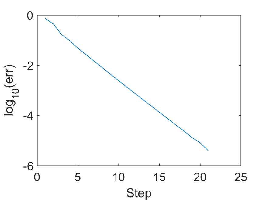
In this section, we demonstrate the convergence of the Sobolev PGD method using some numerical examples. We show that exponential convergence rate is attained both for the original eigenproblem (1) and for its extension (16). We also observe and discuss some interesting phenomena that one may encounter in numerical experiments.

6.1 Gross-Pitaevskii eigenproblem in 2D.

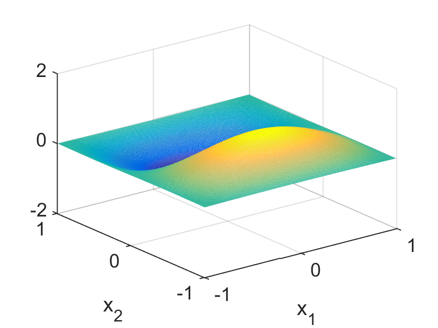
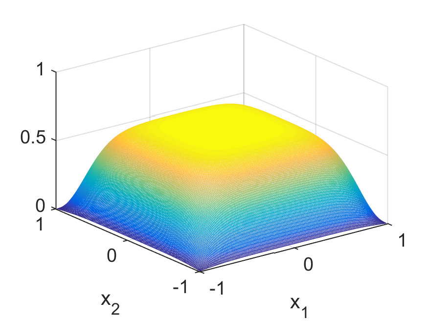
We first look at the Gross-Pitaevskii eigenproblem (1) in two dimensions. Let the domain be Ω=[1,1]22Ωsuperscript112superscript2\Omega=[-1,1]^{2}\subset\mathbb{R}^{2} with Dirichlet boundary condition. The problems are discretized with P1 Lagrange finite element method. The grid is a uniform grid with fixed size h=2282superscript28h=2\cdot 2^{-8} throughout this section.

The first example is a single well potential V(x)=12|x|2𝑉𝑥12superscript𝑥2V(x)=\frac{1}{2}|x|^{2}. It is well known that the Anderson localization [3] is present in this setting. We set β=1𝛽1\beta=1. The initial guess z0subscript𝑧0z_{0} is chosen as the eigenvector corresponding to the smallest eigenvalue of 𝒜0subscript𝒜0{\mathcal{A}}_{0}. It is strictly positive over the whole domain ΩΩ\Omega. The step size is τ=1𝜏1\tau=1.

Figure 1(a) shows the profile of the potential V(x)𝑉𝑥V(x). Figure 1(b) is the profile of the computed ground state with β=1𝛽1\beta=1. Figure 1(c) displays the log H1superscript𝐻1H^{1}-error convergence log10(unvH1/vH1)subscriptlog10subscriptnormsubscript𝑢𝑛𝑣superscript𝐻1subscriptnorm𝑣superscript𝐻1\text{log}_{10}(\|u_{n}-v\|_{H^{1}}/\|v\|_{H^{1}}). It can be seen that the Sobolev PGD converges in just a few steps with an exponential (linear) convergence rate.
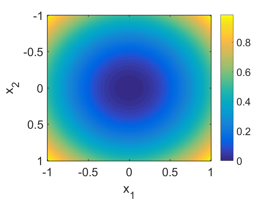
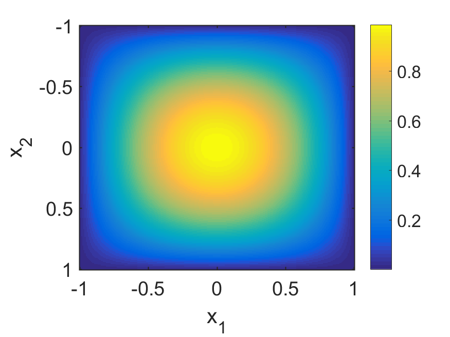
Refer to caption
(a) Single well potential V(x)=12|x|2𝑉𝑥12superscript𝑥2V(x)=\frac{1}{2}|x|^{2}
Refer to caption
(b) Ground state when β=1𝛽1\beta=1
Refer to caption
(c) Log H1superscript𝐻1H^{1}-error convergence
Figure 1: Example of (1) with single well potential V=12|x|2𝑉12superscript𝑥2V=\frac{1}{2}|x|^{2} and β=1𝛽1\beta=1.

By increasing β𝛽\beta, there is a greater nonlinearity in the problem. When β1much-greater-than𝛽1\beta\gg 1, the quartic term β2|u|4𝛽2superscript𝑢4\frac{\beta}{2}|u|^{4} would dominate the energy functional (2). This would be a significant barrier to some traditional methods. Yet the Sobolev PGD remains stable and fast. Figures 2(a) to 2(d) show the log H1superscript𝐻1H^{1}-error convergence and the profiles of the respective ground states with β=10𝛽10\beta=10 and β=100𝛽100\beta=100 respectively. With the Sobolev PGD, there is only a mild increase in the computational complexity, and the iteration still converges exponentially fast as predicted.
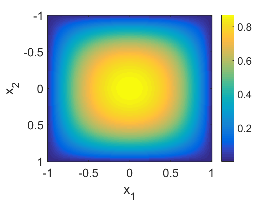
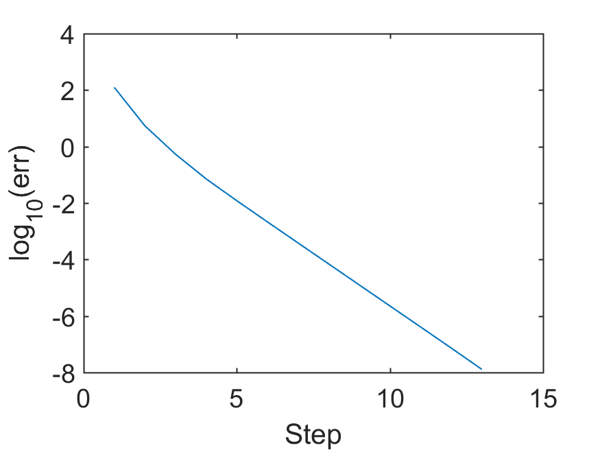
Refer to caption
(a) Ground state when β=10𝛽10\beta=10
Refer to caption
(b) Convergence when β=10𝛽10\beta=10
Refer to caption
(c) Ground state when β=100𝛽100\beta=100
Refer to caption
(d) Convergence when β=100𝛽100\beta=100
Figure 2: Example of (1) with single well potential V=12|x|2𝑉12superscript𝑥2V=\frac{1}{2}|x|^{2} and β=10𝛽10\beta=10 or 100100100.

6.2 Localization under the disordered potential.

The second example is a disordered potential V𝑉V. Its fully discrete counterpart, the randomized potential on the lattice dsuperscript𝑑\mathbb{Z}^{d}, has been extensively studied for its rich behaviour in spectral gaps, exponential localization of eigenstates near the bottom of the spectrum, and implications about the “mobility edge” conjecture in quantum physics and random matrix theory [20, 14].

In our semi-lattice example, the localization of the ground state is also present. In the experiment, V(x)𝑉𝑥V(x) is generated as follows. The extent of disorder is determined by a parameter K=50𝐾50K=50. This means that the domain ΩΩ\Omega is divided into K×K𝐾𝐾K\times K cells. The value of V(x) in each cell is either 111 or 1/K21superscript𝐾21/K^{2}, randomly chosen with equal probability.

Figure 3(a) shows the profile of V(x)𝑉𝑥V(x). Figure 3(b) displays the computed ground state with β=0.5𝛽0.5\beta=0.5. It can be seen that the ground state is concentrated in a small region whose diameter is about a few times the interaction length of the disorder. Figure 3(c) shows the convergence rate of the Sobolev PGD iteration for this example.

To facilitate convergence, we have chosen τ=1.5𝜏1.5\tau=1.5. Although Corollary 3.14 requires a small τ𝜏\tau, in the numerical experiments we find that choosing τ>1𝜏1\tau>1 results in significantly faster convergence. This is in accordance with the empirical findings of [23].
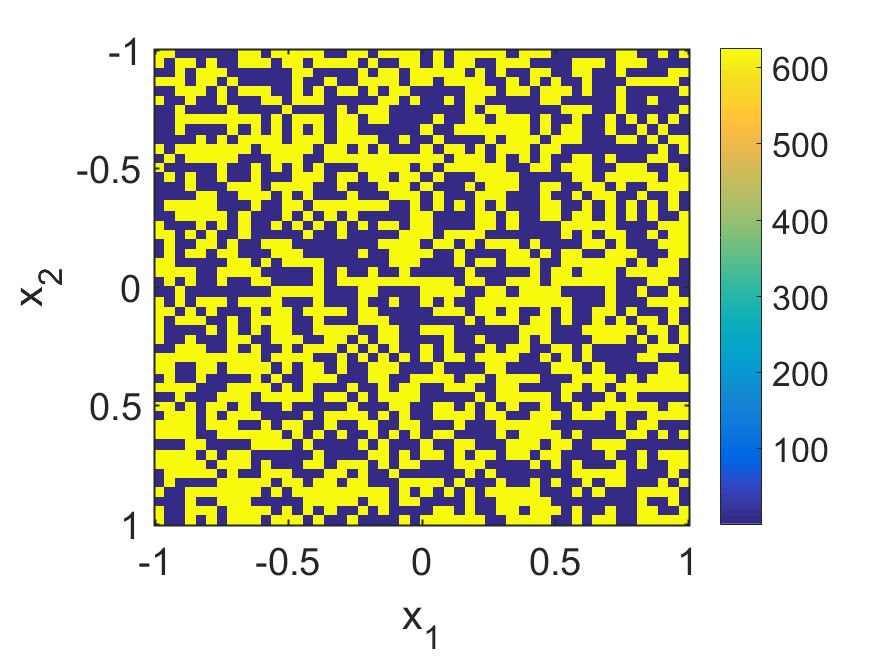
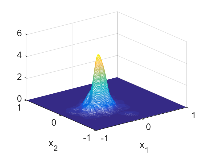
Refer to caption
(a) Profile of the disordered potential
Refer to caption
(b) Profile of the ground state
Refer to caption
(c) Log H1superscript𝐻1H^{1}-error convergence
Figure 3: Example of (1) with a disordered potential and β=0.5𝛽0.5\beta=0.5.

6.3 Asymptotic escape of Sobolev PGD from saddle states.

It is interesting to look at the asymptotic behaviour of the Sobolev gradient descent method if starting from a non-positive initial value. Recall that Corollary 3.14 only ensures exponential convergence to the global ground state from u00subscript𝑢00u_{0}\geq 0. When this condition is violated, it is a priori unknown what the iteration will converge to. It is possible that there are other spurious fixed points, including local minimizers and saddle points. The first-order condition ensures that all these spurious fixed points are eigenstates. But the convergence rate to such points is unknown.

As for the spatially discretized case, the Hilbert manifold \mathcal{M} becomes a Riemannian manifold, and the spectra of the operators become finite. As is proved in [24] and references therein, a random initialization almost surely avoids saddles and converges only to local or global minimizers. It means that if an excited state is a strict saddle point, then a random initialization is very unlikely to converge to that state. As for the spatially continuous case, it is reasonable to expect the same phenomenon, although the analysis could be more difficult due to the infinite dimension of \mathcal{M} and the infinite number of eigenstates.

In the subsequent numerical experiments, we let V(x)=12|x|2𝑉𝑥12superscript𝑥2V(x)=\frac{1}{2}|x|^{2} and β=100𝛽100\beta=100. We will use an example to show that for an excited state that is a strict saddle, it has a very thin converging set close to measure zero. Thus, using Sobolev PGD to compute excited states could be unstable. The accuracy of the computed excited states could be limited.

First, we let the initialization u0subscript𝑢0u_{0} be the second-smallest eigenvector of 𝒜0subscript𝒜0{\mathcal{A}}_{0}. This u0subscript𝑢0u_{0} is positive on half of ΩΩ\Omega and negative on the other half. It is displayed in Figure 4(a). We then let Sobolev PGD iterate a few steps. Figure 4(b) displays the computed state usuperscript𝑢u^{*} when the algorithm stops. Figure 4(c) shows the decrease of the log L2superscript𝐿2L^{2} error with respect to usuperscript𝑢u^{*}. We also compute the manifold Hessian at usuperscript𝑢u^{*} and find that it has at least one negative eigenvalue. Thus usuperscript𝑢u^{*} is a strict saddle state.

Refer to caption
(a) Profile of initial state u0subscript𝑢0u_{0}
Refer to caption
(b) Profile of computed state usuperscript𝑢u^{*}
Refer to caption
(c) Log H1superscript𝐻1H^{1}-error convergence
Figure 4: Behavior of Sobolev PGD for (1) with u00not-greater-than-or-equalssubscript𝑢00u_{0}\not\geq 0.

Next, we add a small perturbation to u0subscript𝑢0u_{0}: we let u^0=u0+ϵηsubscript^𝑢0subscript𝑢0italic-ϵ𝜂\hat{u}_{0}=u_{0}+\epsilon\cdot\eta, where η𝜂\eta is a random noise that is of the same order as u0subscript𝑢0u_{0}, and the parameter ϵitalic-ϵ\epsilon controls the magnitude of noise. We let Sobolev PGD start from u^0subscript^𝑢0\hat{u}_{0} and trace its evolution. What we observe is that, as long as there is a small perturbation, Sobolev PGD escapes from the previous saddle state and converges to the ground state. The parameter ϵitalic-ϵ\epsilon can be chosen as small as 104superscript10410^{-4} and this effect is still present.

Specifically, Figures 5(a) to 5(c) demonstrate the evolution of the log-distance to the precomputed closest excited state usuperscript𝑢u^{*}. We choose ϵ=102italic-ϵsuperscript102\epsilon=10^{-2}, 103superscript10310^{-3}, and 104superscript10410^{-4}, respectively. Saddle escape behavior can be observed in all three cases. We can see that the distance to the excited state first goes down, then goes up. Figure 5(e) show the computed state starting from u^0subscript^𝑢0\hat{u}_{0}, and it is the ground state.

In general, first-order optimization methods, including Sobolev PGD as well as other methods in the gradient descent family, are not good choices for the computation of excited states. They rely on a good enough initialization (like the above u0subscript𝑢0u_{0} without noise) and could suffer from numerical instability issues. One has to resort to other methods if the goal is to obtain high accuracy. We will explore this topic in our upcoming work.
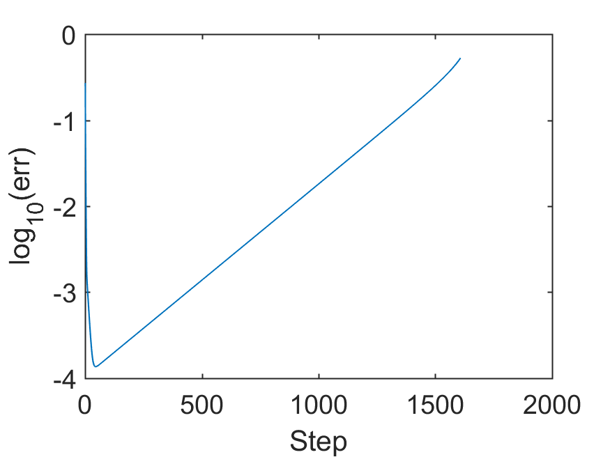
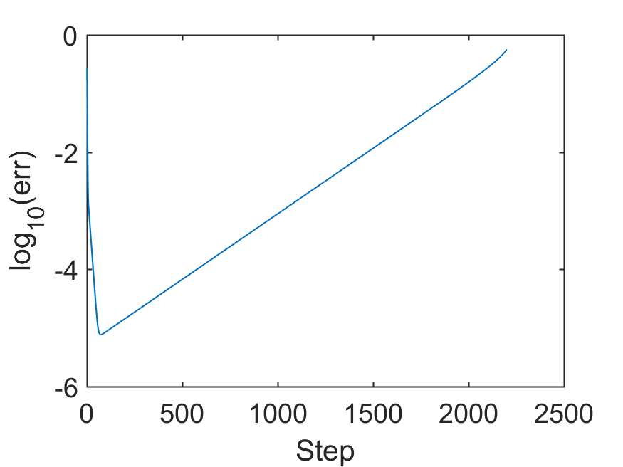
Refer to caption
(a) Noise level ϵ=102italic-ϵsuperscript102\epsilon=10^{-2}
Refer to caption
(b) Noise level ϵ=103italic-ϵsuperscript103\epsilon=10^{-3}
Refer to caption
(c) Noise level ϵ=104italic-ϵsuperscript104\epsilon=10^{-4}
Refer to caption
(d) Profile of u^0=u0+104ηsubscript^𝑢0subscript𝑢0superscript104𝜂\hat{u}_{0}=u_{0}+10^{-4}\eta
Refer to caption
(e) Profile of computed state starting from u^0subscript^𝑢0\hat{u}_{0}
Figure 5: Asymptotic escape from saddle state under small perturbations. Figures (a)-(c) displays the distances to the saddle state usuperscript𝑢u^{*} starting from u^0=u0+ϵηsubscript^𝑢0subscript𝑢0italic-ϵ𝜂\hat{u}_{0}=u_{0}+\epsilon\cdot\eta.

6.4 High order interaction.

We now look at Problem (16) with an extra high order interaction term. This adds additional nonlinearity to the problem. Consider the same domain Ω=[1,1]22Ωsuperscript112superscript2\Omega=[-1,1]^{2}\subset\mathbb{R}^{2} and spatial discretization size h=2282superscript28h=2\cdot 2^{-8}. Let V(x)=12|x|2𝑉𝑥12superscript𝑥2V(x)=\frac{1}{2}|x|^{2} still be the single well potential. The first example is β=10𝛽10\beta=10 and δ=1𝛿1\delta=1. Figure 6(a) shows the log error convergence. The iteration converges in a few steps and shows a good convergence rate.

In the second example, we increase δ𝛿\delta and look at the problem with strong high order interaction. We choose β=100𝛽100\beta=100 and δ=100𝛿100\delta=100. Figure 6(b) shows the log error convergence. The convergence rate is slower but stable.
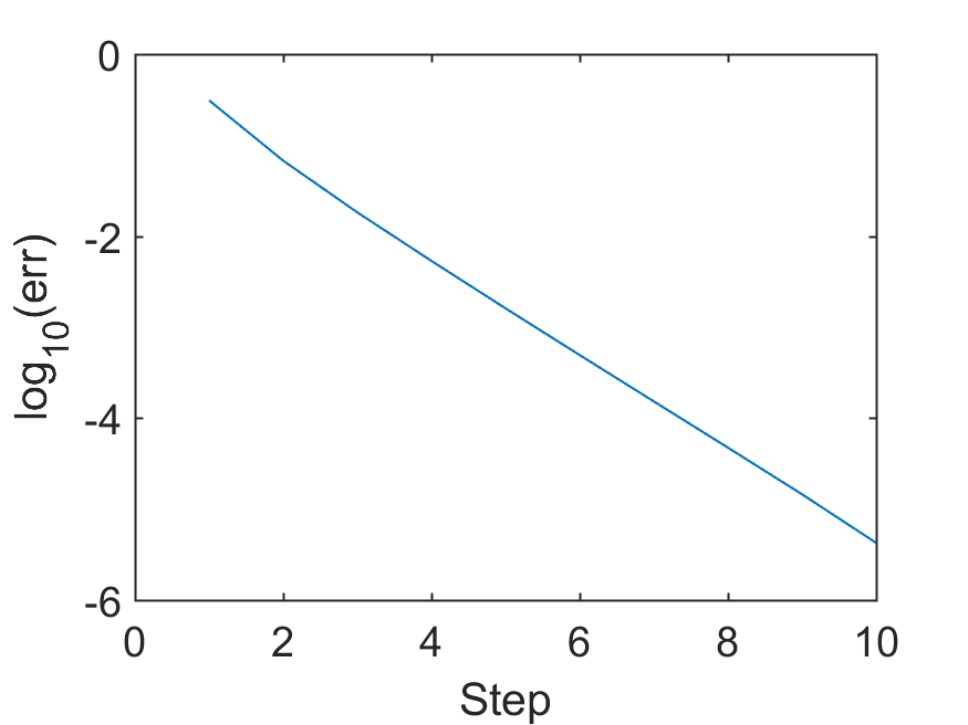
Refer to caption
(a) Convergence when β=10𝛽10\beta=10, δ=1𝛿1\delta=1
Refer to caption
(b) Convergence when β=100𝛽100\beta=100, δ=100𝛿100\delta=100
Figure 6: Examples of (16) with different nonlinear effects

7 Conclusion

In this paper, we analyzed the exponential convergence of the ausubscript𝑎𝑢a_{u}-Sobolev gradient descent method without resorting to the time-continuous gradient flow. To this purpose, we introduced a general convergence tool using the Łojasiewicz inequality, and adapted it to the setting of infinite dimensional Hilbert manifold and mixed norms. By proving the (L), (D) and (S) conditions for the Sobolev PGD, we were able to unveil the mechanism behind the good performance of the Sobolev PGD for the Gross-Pitaevskii eigenproblem (1), which was only empirically observed in previous works.

The success of the Sobolev PGD on the Gross-Pitaevskii eigenproblem inspires us to further explore alternative fast solvers for more general nonlinear eigenproblems and optimizations with high degree objective functions. Our analysis revealed that the essential condition is the “double ground state” property, namely the ground state of the nonlinear problem is also the unique ground state of the linearized operator at that point. This can be rigorously proved in some cases and seems to be true in a number of physical applications of interest based on empirical evidence. Specifically, we showed that this condition is satisfied for a nonlinear Schrödinger eigenproblem with extra high order interaction term. Thus the Sobolev PGD works well for this problem and has superiority over previous methods.

Acknowledgements. This research was in part supported by NSF grants DMS-1912654 and DMS-1907977. The author would like to thank Thomas Y. Hou for the helpful comments on earlier versions of this work, and Zhenzhen Li for introducing the Łojasiewicz inequality to the author. The author would also like to acknowledge the warm hospitality of Oberwolfach Research Institute for Mathematics during the seminar Beyond Numerical Homogenization, where the early ideas of this work started.

References

  • [1] P-A Absil, Robert Mahony, and Rodolphe Sepulchre. Optimization algorithms on matrix manifolds. Princeton University Press, 2009.
  • [2] Mike H Anderson, Jason R Ensher, Michael R Matthews, Carl E Wieman, and Eric A Cornell. Observation of Bose-Einstein condensation in a dilute atomic vapor. Science, pages 198–201, 1995.
  • [3] Philip W Anderson. Absence of diffusion in certain random lattices. Physical review, 109(5):1492, 1958.
  • [4] Weizhu Bao and Yongyong Cai. Mathematical theory and numerical methods for Bose-Einstein condensation. Kinetic & Related Models, 6(1):1–135, 2013.
  • [5] Weizhu Bao, Yongyong Cai, and Xinran Ruan. Ground states of Bose–Einstein condensates with higher order interaction. Physica D: Nonlinear Phenomena, 386:38–48, 2019.
  • [6] Weizhu Bao and Qiang Du. Computing the ground state solution of Bose–Einstein condensates by a normalized gradient flow. SIAM Journal on Scientific Computing, 25(5):1674–1697, 2004.
  • [7] Weizhu Bao and Xinran Ruan. Computing ground states of Bose-Einstein condensates with higher order interaction via a regularized density function formulation. arXiv preprint arXiv:1908.09096, 2019.
  • [8] Eric Cancès, Rachida Chakir, and Yvon Maday. Numerical analysis of nonlinear eigenvalue problems. Journal of Scientific Computing, 45(1-3):90–117, 2010.
  • [9] Eric Cancès, Gaspard Kemlin, and Antoine Levitt. Convergence analysis of direct minimization and self-consistent iterations. arXiv preprint arXiv:2004.09088, 2020.
  • [10] Eric Cancès and Claude Le Bris. On the convergence of SCF algorithms for the Hartree-Fock equations. ESAIM: Mathematical Modelling and Numerical Analysis, 34(4):749–774, 2000.
  • [11] Yuejie Chi, Yue M Lu, and Yuxin Chen. Nonconvex optimization meets low-rank matrix factorization: An overview. IEEE Transactions on Signal Processing, 67(20):5239–5269, 2019.
  • [12] Ionut Danaila and Parimah Kazemi. A new Sobolev gradient method for direct minimization of the Gross–Pitaevskii energy with rotation. SIAM Journal on Scientific Computing, 32(5):2447–2467, 2010.
  • [13] Ionut Danaila and Bartosz Protas. Computation of ground states of the Gross–Pitaevskii functional via Riemannian optimization. SIAM Journal on Scientific Computing, 39(6):B1102–B1129, 2017.
  • [14] Percy Deift et al. Some open problems in random matrix theory and the theory of integrable systems. II. SIGMA. Symmetry, Integrability and Geometry: Methods and Applications, 13:016, 2017.
  • [15] Simone Dovetta, Enrico Serra, and Paolo Tilli. NLS ground states on metric trees: existence results and open questions. arXiv preprint arXiv:1905.00655, 2019.
  • [16] Geneviève Dusson and Yvon Maday. A posteriori analysis of a nonlinear Gross–Pitaevskii-type eigenvalue problem. IMA Journal of Numerical Analysis, 37(1):94–137, 2017.
  • [17] Erwan Faou and Tiphaine Jézéquel. Convergence of a normalized gradient algorithm for computing ground states. IMA Journal of Numerical Analysis, 38(1):360–376, 2018.
  • [18] Rupert L Frank. Ground states of semi-linear pdes. Lecture notes, 2014.
  • [19] Pierre Frankel, Guillaume Garrigos, and Juan Peypouquet. Splitting methods with variable metric for Kurdyka–Łojasiewicz functions and general convergence rates. Journal of Optimization Theory and Applications, 165(3):874–900, 2015.
  • [20] Jürg Fröhlich and Thomas Spencer. Absence of diffusion in the Anderson tight binding model for large disorder or low energy. Communications in Mathematical Physics, 88(2):151–184, 1983.
  • [21] David Gilbarg and Neil S Trudinger. Elliptic partial differential equations of second order. springer, 2015.
  • [22] Patrick Henning, Axel Målqvist, and Daniel Peterseim. Two-level discretization techniques for ground state computations of Bose-Einstein condensates. SIAM Journal on Numerical Analysis, 52(4):1525–1550, 2014.
  • [23] Patrick Henning and Daniel Peterseim. Sobolev gradient flow for the gross–pitaevskii eigenvalue problem: Global convergence and computational efficiency. SIAM Journal on Numerical Analysis, 58(3):1744–1772, 2020.
  • [24] Thomas Y Hou, Zhenzhen Li, and Ziyun Zhang. Analysis of asymptotic escape of strict saddle sets in manifold optimization. arXiv preprint arXiv:1911.12518, 2019.
  • [25] James R Kuttler. Finite difference approximations for eigenvalues of uniformly elliptic operators. SIAM Journal on Numerical Analysis, 7(2):206–232, 1970.
  • [26] Elliott H Lieb, Robert Seiringer, and Jakob Yngvason. Bosons in a trap: A rigorous derivation of the Gross-Pitaevskii energy functional. In The Stability of Matter: From Atoms to Stars, pages 685–697. Springer, 2001.
  • [27] Reinhold Schneider and André Uschmajew. Convergence results for projected line-search methods on varieties of low-rank matrices via Łojasiewicz inequality. SIAM Journal on Optimization, 25(1):622–646, 2015.
  • [28] Haixiang Zhang, Andre Milzarek, Zaiwen Wen, and Wotao Yin. On the geometric analysis of a quartic-quadratic optimization problem under a spherical constraint. arXiv preprint arXiv:1908.00745, 2019.

Appendix A Proofs of technical lemmas

A.1 Proof of Lemma 3.6

Proof.

As for the equivalence between a0\|\cdot\|_{a_{0}} and au\|\cdot\|_{a_{u}}, the second part of the inequality holds for all 0<CE10subscript𝐶𝐸10<C_{E}\leq 1 since u2superscript𝑢2u^{2} is nonnegative. For the first part, by Poincaré inequality, zL22CP|z|H12superscriptsubscriptnorm𝑧superscript𝐿22subscript𝐶𝑃superscriptsubscript𝑧superscript𝐻12\|z\|_{L^{2}}^{2}\leq C_{P}|z|_{H^{1}}^{2} for some domain constant CP=CP(Ω)subscript𝐶𝑃subscript𝐶𝑃ΩC_{P}=C_{P}(\Omega). Thus, we have

za02CEzau2superscriptsubscriptnorm𝑧subscript𝑎02subscript𝐶𝐸superscriptsubscriptnorm𝑧subscript𝑎𝑢2\displaystyle\|z\|_{a_{0}}^{2}-C_{E}\|z\|_{a_{u}}^{2} =(1CE)|z|H12+Ω((1CE)VCEβu2)z2absent1subscript𝐶𝐸superscriptsubscript𝑧superscript𝐻12subscriptΩ1subscript𝐶𝐸𝑉subscript𝐶𝐸𝛽superscript𝑢2superscript𝑧2\displaystyle=(1-C_{E})|z|_{H^{1}}^{2}+\int_{\Omega}((1-C_{E})V-C_{E}\beta u^{2})z^{2}
(1CE)|z|H12CEβΩu2z2absent1subscript𝐶𝐸superscriptsubscript𝑧superscript𝐻12subscript𝐶𝐸𝛽subscriptΩsuperscript𝑢2superscript𝑧2\displaystyle\geq(1-C_{E})|z|_{H^{1}}^{2}-C_{E}\beta\int_{\Omega}u^{2}z^{2}
(1CECEβM02CP)|z|H12,zH01(Ω),CE1.formulae-sequenceabsent1subscript𝐶𝐸subscript𝐶𝐸𝛽superscriptsubscript𝑀02subscript𝐶𝑃superscriptsubscript𝑧superscript𝐻12formulae-sequencefor-all𝑧superscriptsubscript𝐻01Ωsubscript𝐶𝐸1\displaystyle\geq(1-C_{E}-C_{E}\beta M_{0}^{2}C_{P})|z|_{H^{1}}^{2},\qquad\forall z\in H_{0}^{1}(\Omega),\quad C_{E}\leq 1.

Take 0<CE1/(1+βM02CP)0subscript𝐶𝐸11𝛽superscriptsubscript𝑀02subscript𝐶𝑃0<C_{E}\leq 1/(1+\beta M_{0}^{2}C_{P}), then CEzau2za02subscript𝐶𝐸superscriptsubscriptnorm𝑧subscript𝑎𝑢2superscriptsubscriptnorm𝑧subscript𝑎02C_{E}\|z\|_{a_{u}}^{2}\leq\|z\|_{a_{0}}^{2}.

As for the equivalence between au\|\cdot\|_{a_{u}} and H1\|\cdot\|_{H^{1}}, we have

zH12CE~zau2superscriptsubscriptnorm𝑧superscript𝐻12~subscript𝐶𝐸superscriptsubscriptnorm𝑧subscript𝑎𝑢2\displaystyle\|z\|_{H^{1}}^{2}-\widetilde{C_{E}}\|z\|_{a_{u}}^{2} =zH12CE~|z|H12CE~Ω(V+βu2)z2absentsuperscriptsubscriptnorm𝑧superscript𝐻12~subscript𝐶𝐸superscriptsubscript𝑧superscript𝐻12~subscript𝐶𝐸subscriptΩ𝑉𝛽superscript𝑢2superscript𝑧2\displaystyle=\|z\|_{H^{1}}^{2}-\widetilde{C_{E}}|z|_{H^{1}}^{2}-\widetilde{C_{E}}\int_{\Omega}(V+\beta u^{2})z^{2}
(1CE~CE~CP(VL+βM02))|z|H12,zH01(Ω),CE~1.formulae-sequenceabsent1~subscript𝐶𝐸~subscript𝐶𝐸subscript𝐶𝑃subscriptnorm𝑉superscript𝐿𝛽superscriptsubscript𝑀02superscriptsubscript𝑧superscript𝐻12formulae-sequencefor-all𝑧superscriptsubscript𝐻01Ω~subscript𝐶𝐸1\displaystyle\geq\left(1-\widetilde{C_{E}}-\widetilde{C_{E}}C_{P}(\|V\|_{L^{\infty}}+\beta M_{0}^{2})\right)|z|_{H^{1}}^{2},\qquad\forall z\in H_{0}^{1}(\Omega),\quad\widetilde{C_{E}}\leq 1.

Take 0<CE~1/(1+CP(VL+βM02))0~subscript𝐶𝐸11subscript𝐶𝑃subscriptnorm𝑉superscript𝐿𝛽superscriptsubscript𝑀020<\widetilde{C_{E}}\leq 1/(1+C_{P}(\|V\|_{L^{\infty}}+\beta M_{0}^{2})), then CE~zau2zH12~subscript𝐶𝐸superscriptsubscriptnorm𝑧subscript𝑎𝑢2superscriptsubscriptnorm𝑧superscript𝐻12\widetilde{C_{E}}\|z\|_{a_{u}}^{2}\leq\|z\|_{H^{1}}^{2}. On the other hand,

CE~1zau2zH12superscript~subscript𝐶𝐸1superscriptsubscriptnorm𝑧subscript𝑎𝑢2superscriptsubscriptnorm𝑧superscript𝐻12\displaystyle\widetilde{C_{E}}^{-1}\|z\|_{a_{u}}^{2}-\|z\|_{H^{1}}^{2} =(CE~11)|z|H12+CE~1Ω(V+βu2)z2zL2absentsuperscript~subscript𝐶𝐸11superscriptsubscript𝑧superscript𝐻12superscript~subscript𝐶𝐸1subscriptΩ𝑉𝛽superscript𝑢2superscript𝑧2subscriptnorm𝑧superscript𝐿2\displaystyle=(\widetilde{C_{E}}^{-1}-1)|z|_{H^{1}}^{2}+\widetilde{C_{E}}^{-1}\int_{\Omega}(V+\beta u^{2})z^{2}-\|z\|_{L^{2}}
(CP1(CE~11)+CE~1βM021)zL2.absentsuperscriptsubscript𝐶𝑃1superscript~subscript𝐶𝐸11superscript~subscript𝐶𝐸1𝛽superscriptsubscript𝑀021subscriptnorm𝑧superscript𝐿2\displaystyle\geq\left(C_{P}^{-1}(\widetilde{C_{E}}^{-1}-1)+\widetilde{C_{E}}^{-1}\beta M_{0}^{2}-1\right)\|z\|_{L^{2}}.

Take 0<CE~(1+CPβM02)/(1+CP)0~subscript𝐶𝐸1subscript𝐶𝑃𝛽superscriptsubscript𝑀021subscript𝐶𝑃0<\widetilde{C_{E}}\leq(1+C_{P}\beta M_{0}^{2})/(1+C_{P}), then zH12CE~1zau2superscriptsubscriptnorm𝑧superscript𝐻12superscript~subscript𝐶𝐸1superscriptsubscriptnorm𝑧subscript𝑎𝑢2\|z\|_{H^{1}}^{2}\leq\widetilde{C_{E}}^{-1}\|z\|_{a_{u}}^{2}. The final choice of CE~~subscript𝐶𝐸\widetilde{C_{E}} is the smaller of the two. ∎

A.2 Proof of Lemma 3.7

Proof.

For notational simplicity, we allow the constants C,C𝐶superscript𝐶C,\,C^{\prime} to change their meanings through the proof. We also denote

t:=uvH1.assign𝑡subscriptnorm𝑢𝑣superscript𝐻1\displaystyle t:=\|u-v\|_{H^{1}}.

Using the variational form of the eigenvalues, we have

μ1subscript𝜇1\displaystyle\mu_{1} =minzH01(Ω),zL2=1(z,z)au(v,v)au,\displaystyle=\min_{\begin{subarray}{c}z\in H_{0}^{1}(\Omega),\\ \|z\|_{L^{2}}=1\end{subarray}}(z,z)_{a_{u}}\leq(v,v)_{a_{u}},
λ1subscript𝜆1\displaystyle\lambda_{1} =minzH01(Ω),zL2=1(z,z)av(w1,w1)av,\displaystyle=\min_{\begin{subarray}{c}z\in H_{0}^{1}(\Omega),\\ \|z\|_{L^{2}}=1\end{subarray}}(z,z)_{a_{v}}\leq(w_{1},w_{1})_{a_{v}},
λ1+λ2subscript𝜆1subscript𝜆2\displaystyle\lambda_{1}+\lambda_{2} =minz1,z2H01(Ω),z1L2=z2L2=1,z1z2(z1,z1)av+(z2,z2)av(w1,w1)av+(w2,w2)av.\displaystyle=\min_{\begin{subarray}{c}z_{1},z_{2}\in H_{0}^{1}(\Omega),\\ \|z_{1}\|_{L^{2}}=\|z_{2}\|_{L^{2}}=1,\\ z_{1}\perp z_{2}\end{subarray}}(z_{1},z_{1})_{a_{v}}+(z_{2},z_{2})_{a_{v}}\leq(w_{1},w_{1})_{a_{v}}+(w_{2},w_{2})_{a_{v}}.

We will use the above relations to bound the gap between μ1subscript𝜇1\mu_{1} and λ1subscript𝜆1\lambda_{1}, and λ2subscript𝜆2\lambda_{2} and μ2subscript𝜇2\mu_{2}. First, we have

μ1(v,v)ausubscript𝜇1subscript𝑣𝑣subscript𝑎𝑢\displaystyle\mu_{1}\leq(v,v)_{a_{u}} =(v,v)av+Ωβ(u2v2v4)absentsubscript𝑣𝑣subscript𝑎𝑣subscriptΩ𝛽superscript𝑢2superscript𝑣2superscript𝑣4\displaystyle=(v,v)_{a_{v}}+\int_{\Omega}\beta(u^{2}v^{2}-v^{4})
=λ1+Ωβv2(u+v)(uv)absentsubscript𝜆1subscriptΩ𝛽superscript𝑣2𝑢𝑣𝑢𝑣\displaystyle=\lambda_{1}+\int_{\Omega}\beta v^{2}(u+v)(u-v)
λ1+2βM03Ω|uv|absentsubscript𝜆12𝛽superscriptsubscript𝑀03subscriptΩ𝑢𝑣\displaystyle\leq\lambda_{1}+2\beta M_{0}^{3}\int_{\Omega}|u-v|
λ1+C(β,M0,Ω)t.absentsubscript𝜆1𝐶𝛽subscript𝑀0Ω𝑡\displaystyle\leq\lambda_{1}+C(\beta,M_{0},\Omega)\cdot t.

Therefore, there exists C=C(β,M0,Ω)𝐶𝐶𝛽subscript𝑀0ΩC=C(\beta,M_{0},\Omega) such that when tC𝑡𝐶t\leq C,

μ1λ1+16Cv.subscript𝜇1subscript𝜆116subscript𝐶𝑣\displaystyle\mu_{1}\leq\lambda_{1}+\frac{1}{6}C_{v}. (18)

Next, we note that

λ1+λ2(w1,w1)av+(w2,w2)av=(w1,w1)au+(w2,w2)au+Ωβ(v2u2)(w12+w22)=μ1+μ2+Ωβ(v+u)(vu)(w12+w22).subscript𝜆1subscript𝜆2subscriptsubscript𝑤1subscript𝑤1subscript𝑎𝑣subscriptsubscript𝑤2subscript𝑤2subscript𝑎𝑣subscriptsubscript𝑤1subscript𝑤1subscript𝑎𝑢subscriptsubscript𝑤2subscript𝑤2subscript𝑎𝑢subscriptΩ𝛽superscript𝑣2superscript𝑢2superscriptsubscript𝑤12superscriptsubscript𝑤22subscript𝜇1subscript𝜇2subscriptΩ𝛽𝑣𝑢𝑣𝑢superscriptsubscript𝑤12superscriptsubscript𝑤22\displaystyle\begin{split}\lambda_{1}+\lambda_{2}&\leq(w_{1},w_{1})_{a_{v}}+(w_{2},w_{2})_{a_{v}}\\ &=(w_{1},w_{1})_{a_{u}}+(w_{2},w_{2})_{a_{u}}+\int_{\Omega}\beta(v^{2}-u^{2})(w_{1}^{2}+w_{2}^{2})\\ &=\mu_{1}+\mu_{2}+\int_{\Omega}\beta(v+u)(v-u)(w_{1}^{2}+w_{2}^{2}).\end{split} (19)

To estimate w1Lsubscriptnormsubscript𝑤1superscript𝐿\|w_{1}\|_{L^{\infty}}, note that it is the weak solution of

Δw1+Vw1+βu2w1=μ1w1.Δsubscript𝑤1𝑉subscript𝑤1𝛽superscript𝑢2subscript𝑤1subscript𝜇1subscript𝑤1\displaystyle-\Delta w_{1}+Vw_{1}+\beta u^{2}w_{1}=\mu_{1}w_{1}.

Since V,uL(Ω)𝑉𝑢superscript𝐿ΩV,\,u\in L^{\infty}(\Omega), by elliptic regularity, we get

w1H2subscriptnormsubscript𝑤1superscript𝐻2\displaystyle\|w_{1}\|_{H^{2}} C(β,V,M0,Ω)(w1H1+μ1w1L2)absent𝐶𝛽𝑉subscript𝑀0Ωsubscriptnormsubscript𝑤1superscript𝐻1subscript𝜇1subscriptnormsubscript𝑤1superscript𝐿2\displaystyle\leq C(\beta,V,M_{0},\Omega)(\|w_{1}\|_{H^{1}}+\mu_{1}\|w_{1}\|_{L^{2}})
C(β,V,M0,Ω)+C(β,V,M0,Ω)μ1.absent𝐶𝛽𝑉subscript𝑀0Ωsuperscript𝐶𝛽𝑉subscript𝑀0Ωsubscript𝜇1\displaystyle\leq C(\beta,V,M_{0},\Omega)+C^{\prime}(\beta,V,M_{0},\Omega)\cdot\mu_{1}.

When d3𝑑3d\leq 3, using Sobolev embedding, we obtain

w1LC(Ω)w1H2.subscriptnormsubscript𝑤1superscript𝐿𝐶Ωsubscriptnormsubscript𝑤1superscript𝐻2\displaystyle\|w_{1}\|_{L^{\infty}}\leq C(\Omega)\|w_{1}\|_{H^{2}}.

Since we have shown that μ1λ1+Ctsubscript𝜇1subscript𝜆1𝐶𝑡\mu_{1}\leq\lambda_{1}+C\cdot t, putting them together we have

w1LC(β,V,M0,Ω,λ1)+C(β,V,M0,Ω,λ1)t.subscriptnormsubscript𝑤1superscript𝐿𝐶𝛽𝑉subscript𝑀0Ωsubscript𝜆1superscript𝐶𝛽𝑉subscript𝑀0Ωsubscript𝜆1𝑡\displaystyle\|w_{1}\|_{L^{\infty}}\leq C(\beta,V,M_{0},\Omega,\lambda_{1})+C^{\prime}(\beta,V,M_{0},\Omega,\lambda_{1})\cdot t.

Similarly, we can prove that444We omit the details of showing μ2λ2+Ctsubscript𝜇2subscript𝜆2𝐶𝑡\mu_{2}\leq\lambda_{2}+C\cdot t by showing μ1+μ2λ1+λ2+Ctsubscript𝜇1subscript𝜇2subscript𝜆1subscript𝜆2𝐶𝑡\mu_{1}+\mu_{2}\leq\lambda_{1}+\lambda_{2}+C\cdot t using the variational form.

w2LC(β,V,M0,Ω,λ1,λ2)+C(β,V,M0,Ω,λ1,λ2)t.subscriptnormsubscript𝑤2superscript𝐿𝐶𝛽𝑉subscript𝑀0Ωsubscript𝜆1subscript𝜆2superscript𝐶𝛽𝑉subscript𝑀0Ωsubscript𝜆1subscript𝜆2𝑡\displaystyle\|w_{2}\|_{L^{\infty}}\leq C(\beta,V,M_{0},\Omega,\lambda_{1},\lambda_{2})+C^{\prime}(\beta,V,M_{0},\Omega,\lambda_{1},\lambda_{2})\cdot t.

Plugging them back into (19), we have

(w1,w1)av+(w2,w2)avsubscriptsubscript𝑤1subscript𝑤1subscript𝑎𝑣subscriptsubscript𝑤2subscript𝑤2subscript𝑎𝑣\displaystyle(w_{1},w_{1})_{a_{v}}+(w_{2},w_{2})_{a_{v}} μ1+μ2+(C(β,V,M0,Ω,λ1,λ2)+C(β,V,M0,Ω,λ1,λ2)t)2t.absentsubscript𝜇1subscript𝜇2superscript𝐶𝛽𝑉subscript𝑀0Ωsubscript𝜆1subscript𝜆2superscript𝐶𝛽𝑉subscript𝑀0Ωsubscript𝜆1subscript𝜆2𝑡2𝑡\displaystyle\leq\mu_{1}+\mu_{2}+\left(C(\beta,V,M_{0},\Omega,\lambda_{1},\lambda_{2})+C^{\prime}(\beta,V,M_{0},\Omega,\lambda_{1},\lambda_{2})\cdot t\right)^{2}\cdot t.

Therefore, there exists C=C(β,V,M0,Ω,λ1,λ2)𝐶𝐶𝛽𝑉subscript𝑀0Ωsubscript𝜆1subscript𝜆2C=C(\beta,V,M_{0},\Omega,\lambda_{1},\lambda_{2}), such that when tC𝑡𝐶t\leq C,

λ1+λ2μ1+μ2+16Cv.subscript𝜆1subscript𝜆2subscript𝜇1subscript𝜇216subscript𝐶𝑣\displaystyle\lambda_{1}+\lambda_{2}\leq\mu_{1}+\mu_{2}+\frac{1}{6}C_{v}. (20)

Combining (18) and (20), we have

μ1λ1+16Cv,μ2λ213Cv,μ2μ112Cv.formulae-sequencesubscript𝜇1subscript𝜆116subscript𝐶𝑣formulae-sequencesubscript𝜇2subscript𝜆213subscript𝐶𝑣subscript𝜇2subscript𝜇112subscript𝐶𝑣\displaystyle\mu_{1}\leq\lambda_{1}+\frac{1}{6}C_{v},\qquad\mu_{2}\geq\lambda_{2}-\frac{1}{3}C_{v},\qquad\mu_{2}-\mu_{1}\geq\frac{1}{2}C_{v}. (21)

Next, note that

λ1(w1,w1)avsubscript𝜆1subscriptsubscript𝑤1subscript𝑤1subscript𝑎𝑣\displaystyle\lambda_{1}\leq(w_{1},w_{1})_{a_{v}} =(w1,w1)au+Ωβ(v2u2)w12absentsubscriptsubscript𝑤1subscript𝑤1subscript𝑎𝑢subscriptΩ𝛽superscript𝑣2superscript𝑢2superscriptsubscript𝑤12\displaystyle=(w_{1},w_{1})_{a_{u}}+\int_{\Omega}\beta(v^{2}-u^{2})w_{1}^{2}
μ1+C(β,V,M0,Ω)w0L2tabsentsubscript𝜇1𝐶𝛽𝑉subscript𝑀0Ωsuperscriptsubscriptnormsubscript𝑤0superscript𝐿2𝑡\displaystyle\leq\mu_{1}+C(\beta,V,M_{0},\Omega)\|w_{0}\|_{L^{\infty}}^{2}\cdot t
μ1+(C(β,V,M0,Ω)+C(β,V,M0,Ω)t)2t.absentsubscript𝜇1superscript𝐶𝛽𝑉subscript𝑀0Ωsuperscript𝐶𝛽𝑉subscript𝑀0Ω𝑡2𝑡\displaystyle\leq\mu_{1}+(C(\beta,V,M_{0},\Omega)+C^{\prime}(\beta,V,M_{0},\Omega)\cdot t)^{2}\cdot t.

Therefore, there exists C=C(β,V,M0,Ω,λ1)𝐶𝐶𝛽𝑉subscript𝑀0Ωsubscript𝜆1C=C(\beta,V,M_{0},\Omega,\lambda_{1}) such that when tC𝑡𝐶t\leq C,

λ1μ1+16Cv.subscript𝜆1subscript𝜇116subscript𝐶𝑣\displaystyle\lambda_{1}\leq\mu_{1}+\frac{1}{6}C_{v}. (22)

Equations (18), (21) and (22) contain all the relations between λ1,λ2,μ1subscript𝜆1subscript𝜆2subscript𝜇1\lambda_{1},\,\lambda_{2},\,\mu_{1}, and μ2subscript𝜇2\mu_{2} that we will need.

Since {wi}i=1superscriptsubscriptsubscript𝑤𝑖𝑖1\{w_{i}\}_{i=1}^{\infty} forms an orthonormal basis of H01(Ω)superscriptsubscript𝐻01ΩH_{0}^{1}(\Omega), in order to estimate uw1L2subscriptnorm𝑢subscript𝑤1superscript𝐿2\|u-w_{1}\|_{L^{2}}, it suffices to bound (u,u)auμ1subscript𝑢𝑢subscript𝑎𝑢subscript𝜇1(u,u)_{a_{u}}-\mu_{1}. Note that

(u,u)auλ1subscript𝑢𝑢subscript𝑎𝑢subscript𝜆1\displaystyle(u,u)_{a_{u}}-\lambda_{1} =(u,u)au(v,v)avabsentsubscript𝑢𝑢subscript𝑎𝑢subscript𝑣𝑣subscript𝑎𝑣\displaystyle=(u,u)_{a_{u}}-(v,v)_{a_{v}}
=(u,u)au(v,v)au+Ωβ(u2v2v4)absentsubscript𝑢𝑢subscript𝑎𝑢subscript𝑣𝑣subscript𝑎𝑢subscriptΩ𝛽superscript𝑢2superscript𝑣2superscript𝑣4\displaystyle=(u,u)_{a_{u}}-(v,v)_{a_{u}}+\int_{\Omega}\beta(u^{2}v^{2}-v^{4})
(uau+vau)uvau+Ωβv2(u+v)(uv)absentsubscriptnorm𝑢subscript𝑎𝑢subscriptnorm𝑣subscript𝑎𝑢subscriptnorm𝑢𝑣subscript𝑎𝑢subscriptΩ𝛽superscript𝑣2𝑢𝑣𝑢𝑣\displaystyle\leq(\|u\|_{a_{u}}+\|v\|_{a_{u}})\cdot\|u-v\|_{a_{u}}+\int_{\Omega}\beta v^{2}(u+v)(u-v)
C(β,V,M0,Ω)(uH1+vH1)uvH1+Ωβv2(u+v)(uv)absent𝐶𝛽𝑉subscript𝑀0Ωsubscriptnorm𝑢superscript𝐻1subscriptnorm𝑣superscript𝐻1subscriptnorm𝑢𝑣superscript𝐻1subscriptΩ𝛽superscript𝑣2𝑢𝑣𝑢𝑣\displaystyle\leq C(\beta,V,M_{0},\Omega)(\|u\|_{H^{1}}+\|v\|_{H^{1}})\cdot\|u-v\|_{H^{1}}+\int_{\Omega}\beta v^{2}(u+v)(u-v)
C(β,V,M0,Ω)t.absent𝐶𝛽𝑉subscript𝑀0Ω𝑡\displaystyle\leq C(\beta,V,M_{0},\Omega)\cdot t.

The fourth inequality uses the norm equivalence in Lemma 3.6. Thus, there exists C=C(β,V,M0,Ω)𝐶𝐶𝛽𝑉subscript𝑀0ΩC=C(\beta,V,M_{0},\Omega), such that when tC𝑡𝐶t\leq C,

(u,u)auλ1112Cv.subscript𝑢𝑢subscript𝑎𝑢subscript𝜆1112subscript𝐶𝑣\displaystyle(u,u)_{a_{u}}-\lambda_{1}\leq\frac{1}{12}C_{v}. (23)

Combining (21), (22) and (23), we have

(u,u)auμ114Cv12(μ2μ1).subscript𝑢𝑢subscript𝑎𝑢subscript𝜇114subscript𝐶𝑣12subscript𝜇2subscript𝜇1\displaystyle(u,u)_{a_{u}}-\mu_{1}\leq\frac{1}{4}C_{v}\leq\frac{1}{2}(\mu_{2}-\mu_{1}).

Assume that u=i=1ciwi𝑢superscriptsubscript𝑖1subscript𝑐𝑖subscript𝑤𝑖u=\sum_{i=1}^{\infty}c_{i}w_{i}, where i=1ci2=1superscriptsubscript𝑖1superscriptsubscript𝑐𝑖21\sum_{i=1}^{\infty}c_{i}^{2}=1. Then we get

(u,u)auμ1=i=1ci2μiμ1c12μ1+i=2ci2μ2μ1=(1c12)(μ2μ1).subscript𝑢𝑢subscript𝑎𝑢subscript𝜇1superscriptsubscript𝑖1superscriptsubscript𝑐𝑖2subscript𝜇𝑖subscript𝜇1superscriptsubscript𝑐12subscript𝜇1superscriptsubscript𝑖2superscriptsubscript𝑐𝑖2subscript𝜇2subscript𝜇11superscriptsubscript𝑐12subscript𝜇2subscript𝜇1\displaystyle(u,u)_{a_{u}}-\mu_{1}=\sum_{i=1}^{\infty}c_{i}^{2}\mu_{i}-\mu_{1}\geq c_{1}^{2}\mu_{1}+\sum_{i=2}^{\infty}c_{i}^{2}\mu_{2}-\mu_{1}=(1-c_{1}^{2})(\mu_{2}-\mu_{1}).

Since (u,u)auμ112(μ2μ1)subscript𝑢𝑢subscript𝑎𝑢subscript𝜇112subscript𝜇2subscript𝜇1(u,u)_{a_{u}}-\mu_{1}\leq\frac{1}{2}(\mu_{2}-\mu_{1}), we have

1c1212,|c1|12.formulae-sequence1superscriptsubscript𝑐1212subscript𝑐112\displaystyle 1-c_{1}^{2}\leq\frac{1}{2},\qquad|c_{1}|\geq\frac{1}{\sqrt{2}}.

If c11/2subscript𝑐112c_{1}\leq-1/\sqrt{2}, we can use w1subscript𝑤1-w_{1} to replace w1subscript𝑤1w_{1}. Thus, we always have c11/2subscript𝑐112c_{1}\geq 1/\sqrt{2}. This gives

uw1L2=22c122<1.subscriptnorm𝑢subscript𝑤1superscript𝐿222subscript𝑐1221\displaystyle\|u-w_{1}\|_{L^{2}}=\sqrt{2-2c_{1}}\leq\sqrt{2-\sqrt{2}}<1.

In other words, s22𝑠22s\leq\sqrt{2-\sqrt{2}}. The constant C𝐶C in the statement of the lemma is the smallest of all the constants C𝐶C, Csuperscript𝐶C^{\prime} in the proof. Since λ2=λ1+Cvsubscript𝜆2subscript𝜆1subscript𝐶𝑣\lambda_{2}=\lambda_{1}+C_{v}, the dependence on λ2subscript𝜆2\lambda_{2} is the dependence on Cvsubscript𝐶𝑣C_{v}. ∎

A.3 Proof of Lemma 3.8

Proof.

Since μ2subscript𝜇2\mu_{2} is strictly greater than μ1subscript𝜇1\mu_{1}, we can split 𝒜𝒜{\mathcal{A}} and u𝑢u as

𝒜=𝒜(1)+𝒜(2),𝒜(1)=𝒜Pw1,𝒜(2)=𝒜Pw1,formulae-sequence𝒜superscript𝒜1superscript𝒜2formulae-sequencesuperscript𝒜1𝒜subscript𝑃subscript𝑤1superscript𝒜2𝒜superscriptsubscript𝑃subscript𝑤1perpendicular-to\displaystyle{\mathcal{A}}={\mathcal{A}}^{(1)}+{\mathcal{A}}^{(2)},\quad{\mathcal{A}}^{(1)}={\mathcal{A}}P_{w_{1}},\quad{\mathcal{A}}^{(2)}={\mathcal{A}}P_{w_{1}}^{\perp},
u=u(1)+u(2),u(1)=Pw1u,u(2)=Pw1u.formulae-sequence𝑢superscript𝑢1superscript𝑢2formulae-sequencesuperscript𝑢1subscript𝑃subscript𝑤1𝑢superscript𝑢2superscriptsubscript𝑃subscript𝑤1perpendicular-to𝑢\displaystyle u=u^{(1)}+u^{(2)},\quad u^{(1)}=P_{w_{1}}u,\quad u^{(2)}=P_{w_{1}}^{\perp}u.

Here Pw1subscript𝑃subscript𝑤1P_{w_{1}} is the orthogonal projection onto the subspace of w1subscript𝑤1w_{1} under the L2superscript𝐿2L^{2} inner product, and Pw1=idPw1superscriptsubscript𝑃subscript𝑤1perpendicular-to𝑖𝑑subscript𝑃subscript𝑤1P_{w_{1}}^{\perp}=id-P_{w_{1}}. Then 𝒜(1)u(1)=μ1u(1)superscript𝒜1superscript𝑢1subscript𝜇1superscript𝑢1{\mathcal{A}}^{(1)}u^{(1)}=\mu_{1}u^{(1)}, and (u(2),u(2))𝒜(2)μ2u(2)L22subscriptsuperscript𝑢2superscript𝑢2superscript𝒜2subscript𝜇2superscriptsubscriptnormsuperscript𝑢2superscript𝐿22(u^{(2)},u^{(2)})_{{\mathcal{A}}^{(2)}}\geq\mu_{2}\|u^{(2)}\|_{L^{2}}^{2} since u(2)w1perpendicular-tosuperscript𝑢2subscript𝑤1u^{(2)}\perp w_{1}. By definition of 𝒢𝒢\mathcal{G}, (u,𝒢v)𝒜=(u,v)L2subscript𝑢𝒢𝑣𝒜subscript𝑢𝑣superscript𝐿2(u,\mathcal{G}v)_{\mathcal{A}}=(u,v)_{L^{2}} for any u,vX𝑢𝑣𝑋u,v\in X. We have

(u,𝒢u(1))L2subscript𝑢𝒢superscript𝑢1superscript𝐿2\displaystyle(u,\mathcal{G}u^{(1)})_{L^{2}} =μ11u(1)L22,absentsuperscriptsubscript𝜇11subscriptsuperscriptnormsuperscript𝑢12superscript𝐿2\displaystyle=\mu_{1}^{-1}\|u^{(1)}\|^{2}_{L^{2}},
(u,𝒢u(2))L2subscript𝑢𝒢superscript𝑢2superscript𝐿2\displaystyle(u,\mathcal{G}u^{(2)})_{L^{2}} =(u(1),𝒢u(2))L2+(u(2),𝒢u(2))L2=(u(2),𝒢u(2))L2,absentsubscriptsuperscript𝑢1𝒢superscript𝑢2superscript𝐿2subscriptsuperscript𝑢2𝒢superscript𝑢2superscript𝐿2subscriptsuperscript𝑢2𝒢superscript𝑢2superscript𝐿2\displaystyle=(u^{(1)},\mathcal{G}u^{(2)})_{L^{2}}+(u^{(2)},\mathcal{G}u^{(2)})_{L^{2}}=(u^{(2)},\mathcal{G}u^{(2)})_{L^{2}},
(u(2),𝒢u(2))L2subscriptsuperscript𝑢2𝒢superscript𝑢2superscript𝐿2\displaystyle(u^{(2)},\mathcal{G}u^{(2)})_{L^{2}} =(𝒢u(2),𝒢u(2))𝒜μ2𝒢u(2)L22absentsubscript𝒢superscript𝑢2𝒢superscript𝑢2𝒜subscript𝜇2subscriptsuperscriptnorm𝒢superscript𝑢22superscript𝐿2\displaystyle=(\mathcal{G}u^{(2)},\mathcal{G}u^{(2)})_{{\mathcal{A}}}\geq\mu_{2}\|\mathcal{G}u^{(2)}\|^{2}_{L^{2}}
=μ2u(2)L22(𝒢u(2)L22u(2)L22)μ2u(2)L22(u(2),𝒢u(2))L22,absentsubscript𝜇2subscriptsuperscriptnormsuperscript𝑢22superscript𝐿2subscriptsuperscriptnorm𝒢superscript𝑢22superscript𝐿2subscriptsuperscriptnormsuperscript𝑢22superscript𝐿2subscript𝜇2subscriptsuperscriptnormsuperscript𝑢22superscript𝐿2subscriptsuperscriptsuperscript𝑢2𝒢superscript𝑢22superscript𝐿2\displaystyle=\mu_{2}\|u^{(2)}\|^{-2}_{L^{2}}\cdot(\|\mathcal{G}u^{(2)}\|^{2}_{L^{2}}\|u^{(2)}\|^{2}_{L^{2}})\geq\mu_{2}\|u^{(2)}\|^{-2}_{L^{2}}\cdot(u^{(2)},\mathcal{G}u^{(2)})^{2}_{L^{2}},
i.e., (u,𝒢u(2))L2μ21u(2)L22.subscript𝑢𝒢superscript𝑢2superscript𝐿2superscriptsubscript𝜇21superscriptsubscriptnormsuperscript𝑢2superscript𝐿22\displaystyle(u,\mathcal{G}u^{(2)})_{L^{2}}\leq\mu_{2}^{-1}\|u^{(2)}\|_{L^{2}}^{2}.

Therefore, the objective inequality is transformed into

CL((u,u)𝒜1(u,𝒢u)L2)((u,u)𝒜(w1,w1)𝒜)subscript𝐶𝐿subscript𝑢𝑢𝒜1subscript𝑢𝒢𝑢superscript𝐿2subscript𝑢𝑢𝒜subscriptsubscript𝑤1subscript𝑤1𝒜\displaystyle C_{L}\left((u,u)_{\mathcal{A}}-\frac{1}{(u,\mathcal{G}u)_{L^{2}}}\right)-\left((u,u)_{\mathcal{A}}-(w_{1},w_{1})_{\mathcal{A}}\right)
=(CL1)(u,u)𝒜CL(u,𝒢u)L2+μ1absentsubscript𝐶𝐿1subscript𝑢𝑢𝒜subscript𝐶𝐿subscript𝑢𝒢𝑢superscript𝐿2subscript𝜇1\displaystyle=(C_{L}-1)(u,u)_{\mathcal{A}}-\frac{C_{L}}{(u,\mathcal{G}u)_{L^{2}}}+\mu_{1}
=(CL1)((u(1),u(1))𝒜(1)+(u(2),u(2))𝒜(2))CL(u,𝒢u(1))L2+(u,𝒢u(2))L2+μ1absentsubscript𝐶𝐿1subscriptsuperscript𝑢1superscript𝑢1superscript𝒜1subscriptsuperscript𝑢2superscript𝑢2superscript𝒜2subscript𝐶𝐿subscript𝑢𝒢superscript𝑢1superscript𝐿2subscript𝑢𝒢superscript𝑢2superscript𝐿2subscript𝜇1\displaystyle=(C_{L}-1)((u^{(1)},u^{(1)})_{{\mathcal{A}}^{(1)}}+(u^{(2)},u^{(2)})_{{\mathcal{A}}^{(2)}})-\frac{C_{L}}{(u,\mathcal{G}u^{(1)})_{L^{2}}+(u,\mathcal{G}u^{(2)})_{L^{2}}}+\mu_{1}
(CL1)(μ1u(1)L22+μ2u(2)L22)CLμ11u(1)L22+μ21u(2)L22+μ1absentsubscript𝐶𝐿1subscript𝜇1subscriptsuperscriptnormsuperscript𝑢12superscript𝐿2subscript𝜇2subscriptsuperscriptnormsuperscript𝑢22superscript𝐿2subscript𝐶𝐿superscriptsubscript𝜇11subscriptsuperscriptnormsuperscript𝑢12superscript𝐿2superscriptsubscript𝜇21superscriptsubscriptnormsuperscript𝑢2superscript𝐿22subscript𝜇1\displaystyle\geq(C_{L}-1)(\mu_{1}\|u^{(1)}\|^{2}_{L^{2}}+\mu_{2}\|u^{(2)}\|^{2}_{L^{2}})-\frac{C_{L}}{\mu_{1}^{-1}\|u^{(1)}\|^{2}_{L^{2}}+\mu_{2}^{-1}\|u^{(2)}\|_{L^{2}}^{2}}+\mu_{1}
=(CL1)(μ1+(μ2μ1)u(2)L22)CLμ1μ2μ2+(μ1μ2)u(2)L22+μ1absentsubscript𝐶𝐿1subscript𝜇1subscript𝜇2subscript𝜇1subscriptsuperscriptnormsuperscript𝑢22superscript𝐿2subscript𝐶𝐿subscript𝜇1subscript𝜇2subscript𝜇2subscript𝜇1subscript𝜇2superscriptsubscriptnormsuperscript𝑢2superscript𝐿22subscript𝜇1\displaystyle=(C_{L}-1)(\mu_{1}+(\mu_{2}-\mu_{1})\|u^{(2)}\|^{2}_{L^{2}})-\frac{C_{L}\mu_{1}\mu_{2}}{\mu_{2}+(\mu_{1}-\mu_{2})\|u^{(2)}\|_{L^{2}}^{2}}+\mu_{1}
=(μ2μ1)((CL1)μ2CLμ1)u(2)L22(CL1)(μ2μ1)u(2)L24μ2+(μ1μ2)u(2)L22.absentsubscript𝜇2subscript𝜇1subscript𝐶𝐿1subscript𝜇2subscript𝐶𝐿subscript𝜇1superscriptsubscriptnormsuperscript𝑢2superscript𝐿22subscript𝐶𝐿1subscript𝜇2subscript𝜇1superscriptsubscriptnormsuperscript𝑢2superscript𝐿24subscript𝜇2subscript𝜇1subscript𝜇2superscriptsubscriptnormsuperscript𝑢2superscript𝐿22\displaystyle=(\mu_{2}-\mu_{1})\frac{((C_{L}-1)\mu_{2}-C_{L}\mu_{1})\|u^{(2)}\|_{L^{2}}^{2}-(C_{L}-1)(\mu_{2}-\mu_{1})\|u^{(2)}\|_{L^{2}}^{4}}{\mu_{2}+(\mu_{1}-\mu_{2})\|u^{(2)}\|_{L^{2}}^{2}}.

We look for CLsubscript𝐶𝐿C_{L} and u𝑢u such that the above is greater than or equal to 0. In fact, for any CL>1subscript𝐶𝐿1C_{L}>1, if

0u(2)L22(CL1)μ2CLμ1(CL1)(μ2μ1),0superscriptsubscriptnormsuperscript𝑢2superscript𝐿22subscript𝐶𝐿1subscript𝜇2subscript𝐶𝐿subscript𝜇1subscript𝐶𝐿1subscript𝜇2subscript𝜇1\displaystyle 0\leq\|u^{(2)}\|_{L^{2}}^{2}\leq\frac{(C_{L}-1)\mu_{2}-C_{L}\mu_{1}}{(C_{L}-1)(\mu_{2}-\mu_{1})},

then this is satisfied. Note that uv1L2ssubscriptnorm𝑢subscript𝑣1superscript𝐿2𝑠\|u-v_{1}\|_{L^{2}}\leq{s} implies u(2)L22s2superscriptsubscriptnormsuperscript𝑢2superscript𝐿22superscript𝑠2\|u^{(2)}\|_{L^{2}}^{2}\leq{s}^{2}. So the requirement on CLsubscript𝐶𝐿C_{L} is

CL1+μ2(μ2μ1)(1s2).subscript𝐶𝐿1subscript𝜇2subscript𝜇2subscript𝜇11superscript𝑠2\displaystyle C_{L}\geq 1+\frac{\mu_{2}}{(\mu_{2}-\mu_{1})(1-{s}^{2})}.

A.4 Proof of Lemma 5.2

Proof.

The main idea of the proof is the same as that of Lemma 3.7 so we only point out their differences here. For example, to estimate μ1λ1subscript𝜇1subscript𝜆1\mu_{1}-\lambda_{1}, we have

μ1(v,v)ausubscript𝜇1subscript𝑣𝑣subscript𝑎𝑢\displaystyle\mu_{1}\leq(v,v)_{a_{u}} =(v,v)av+Ωβ(u2v2v4)+Ωδ(((uv)2(v2)2))\displaystyle=(v,v)_{a_{v}}+\int_{\Omega}\beta(u^{2}v^{2}-v^{4})+\int_{\Omega}\delta\left((\nabla(uv)^{2}-\nabla(v^{2})^{2})\right)
=λ1+Ωβv2(u+v)(uv)+Ωδ((uv)+(v2))((uv)(v2)).absentsubscript𝜆1subscriptΩ𝛽superscript𝑣2𝑢𝑣𝑢𝑣subscriptΩ𝛿𝑢𝑣superscript𝑣2𝑢𝑣superscript𝑣2\displaystyle=\lambda_{1}+\int_{\Omega}\beta v^{2}(u+v)(u-v)+\int_{\Omega}\delta(\nabla(uv)+\nabla(v^{2}))(\nabla(uv)-\nabla(v^{2})).

The second term is bounded in the same way as the proof of Lemma 3.7. Only the third term containing high-order interaction is new. To bound the third term, we note that

Ωδ((uv)+(v2))((uv)(v2))subscriptΩ𝛿𝑢𝑣superscript𝑣2𝑢𝑣superscript𝑣2\displaystyle\int_{\Omega}\delta(\nabla(uv)+\nabla(v^{2}))(\nabla(uv)-\nabla(v^{2}))
=δΩ(vu+uv+2vv)(vu+uv2vv)absent𝛿subscriptΩ𝑣𝑢𝑢𝑣2𝑣𝑣𝑣𝑢𝑢𝑣2𝑣𝑣\displaystyle=\delta\int_{\Omega}(v\nabla u+u\nabla v+2v\nabla v)(v\nabla u+u\nabla v-2v\nabla v)
4δM0M1Ω|vu+uv2vv|absent4𝛿subscript𝑀0subscript𝑀1subscriptΩ𝑣𝑢𝑢𝑣2𝑣𝑣\displaystyle\leq 4\delta M_{0}M_{1}\int_{\Omega}\left|v\nabla u+u\nabla v-2v\nabla v\right|
=4δM0M1Ω|v(uv)+(uv)v|absent4𝛿subscript𝑀0subscript𝑀1subscriptΩ𝑣𝑢𝑣𝑢𝑣𝑣\displaystyle=4\delta M_{0}M_{1}\int_{\Omega}\left|v(\nabla u-\nabla v)+(u-v)\nabla v\right|
C(δ,M0,M1,Ω)uvH1.absent𝐶𝛿subscript𝑀0subscript𝑀1Ωsubscriptnorm𝑢𝑣superscript𝐻1\displaystyle\leq C(\delta,M_{0},M_{1},\Omega)\|u-v\|_{H^{1}}.

Similar bounds can be obtained in the estimation of (λ1+λ2)(μ1+μ2)subscript𝜆1subscript𝜆2subscript𝜇1subscript𝜇2(\lambda_{1}+\lambda_{2})-(\mu_{1}+\mu_{2}), λ1μ1subscript𝜆1subscript𝜇1\lambda_{1}-\mu_{1}, and (u,u)auμ1subscript𝑢𝑢subscript𝑎𝑢subscript𝜇1(u,u)_{a_{u}}-\mu_{1}. The dependence of the constant C𝐶C only has two additional dependencies which are δ𝛿\delta and M1subscript𝑀1M_{1}. ∎