Qualitative methods in condensed matter physics

Abstract

Expanding on our former hypothesis that, in the current information age, teaching physics should become more intuition-based and aiming at pattern recognition skills, we present multiple examples of qualitative methods in condensed matter physics. They include the subjects of phonons, thermal and electronic properties of matter, electron-phonon interactions and some properties of semiconductors.

I Introduction

This manuscript expands on our recent premise karpov2019 that teaching physics in the information age should become more intuitive and induction-driven rather than guided by memorization and principles assumed by deductive learning. The underlying reality is that the standard physics curriculum information is now available at our fingertips through smartphones, computers, etc. That information avalanche is accentuating the need for efficient pattern-recognition and result evaluation skills.

Our implied inductive learning (i. e. from examples) does not necessarily lead to generalizations (making the subsequent learning deductive howpeoplelearn ), which are neither sufficient nor necessary. Examples of inductive learning without generalization include language learning in children, sports training, professionally successful problem solving based on “experience”, etc. In a similar manner, when learning the language of science -in this case physics- our brain’s functionality is geared toward induction through the processes of pattern recognition and neural network training.

A strong ‘experimental’ support for the latter insight comes from the modern understanding of neural networks that demonstrates how such learning can be prevailing and useful. Indeed, studying the available machine learning and artificial intelligence operations does not offer a possibility to determine how the system makes its decision: all in all, it appears as a result of forming certain connections between the system neurons achieved by trial and error. The resulting neural nets are created without a prior knowledge, neither can they be translated into operational theoretical deduction.

The pathway toward developing inductive learning abilities taken in our preceding work karpov2019 is that of practicing various qualitative methods. They are fast and intuitive, boosting the learner’s self-esteem, benefiting both students and professionals in navigating the overwhelming amount of information. That preceding work was limited to qualitative methods in quantum mechanics, which is a well-established homogeneous field. The current manuscript aims at expanding over a different type of discipline, condensed matter physics, which is both multi-faceted (phonons, electrons, magnetism, elasticity, thermodynamics, etc.) and multi-format (condensed matter theory, material sciences, physics of semiconductors, electronic materials, etc.) yeh Developing inductive learning abilities (pattern recognition, approximations, back of the envelope calculations, etc.) presents a formidable challenge. It is met here with the same approach as before: demonstrating multiple patterns of qualitative analyses for various problems. By no means can we claim that this approach is sufficient; however, we hope it will be useful in developing such abilities in the field of condensed matter sciences.

But how can one make a representative selection of topics from the almost infinite number of condensed matter possibilities? Our approach here favors taste-based topics allowing qualitative methods. (We note parenthetically that many problems in condensed matter would not allow qualitative methods, such as e. g. energy analyses of particular microscopic configurations in solids. The ability to recognize ‘a smell’ of qualitatively treatable problems appears to be a useful skill, and that can be instilled by examples.) Other contributions of condensed matter subjects attainable to qualitative methods are called upon for the benefit of the learners. The material that follows will remain an illustration.

One other goal here is to bring a flavor of condensed matter physics and sketch its skeleton for those without any significant background. We hope that such a sketch and intuition will allow faster progress by then consciously collecting and organizing relevant information from other sources.

We shall end this introduction admitting that the standard condensed matter curricula will remain utterly important in professional development. Our additions here will just facilitate their learning making the subject more intuitive and paving ways to inductive learning in other subfields of condensed matter physics.

II The ultimate simplicity models

It is obvious that a single atom cannot serve as a model of condensed matter for $N\gg 1$ atoms. However, two atoms do represent some basic properties of condensed matter when they form a diatomic molecule, since the latter possess a variety of relevant characteristics: binding energy, elasticity and anharmonicity, vibrational frequency, specific heat, etc. These characteristics are all practically significant determining the range of various material applications.

Another useful simplistic model in condensed matter physics is that of two level systems, which generally does not specify the physical nature of energy spectrum limited to the irreducible minimum of just two (a one level model is of no interest, not allowing any transitions in the system). Oftentimes, the two level system properties exhibit themselves in objects with much more complex energy spectra; in other cases, the two-level structure per se is dictated by the underlying physics.

The toy models below represent a useful example of simplifications where phenomena observed in complex systems (solids) are traced down to irreducibly primitive objects: two atoms or two energy levels. In a sense, they show how the number of two (but not one!) may be large enough to reveal the physics of many-body systems.

II.1 Diatomic model

This simplistic model introduces a number of properties central in condensed matter physics: binding energies, adiabatic description, harmonic vibrations, elasticity and anharmonic effects, and deformation potential interaction.

We start with recalling the shape and origin of a diatomic interaction in Fig. 1 where the potential energy is a sum of two contributions presented by dashed lines and illustrated in the insets. One of them is the repulsion between atomic cores $E_{aa}$ (for example between two protons in the case of hydrogen molecule). Another one, $E_{ea}$ is the attraction due to forming a valence bond with energy corresponding to lowest of two split levels originating from quantum tunneling of the valence electron between two atoms. We further consider that phenomenon in Sec. IV.1.1 below.

The latter energy is written in the adiabatic approximation ashcroft where it is a function of atomic coordinates only but not their velocities. (We recall that the adiabatic approximation calculates the electron energy at a given instantaneous atomic configuration, neglecting atomic motion as very slow due to their heavy masses compared to that of electrons.) The corresponding atomic energy is calculated as the average over the electron wave function corresponding to a given set of atomic positions. The small parameter describing the slowness of atomic systems compared to that of electrons is related to the ratio of the electronic and atomic masses as demonstrated in Eq. (2) below.

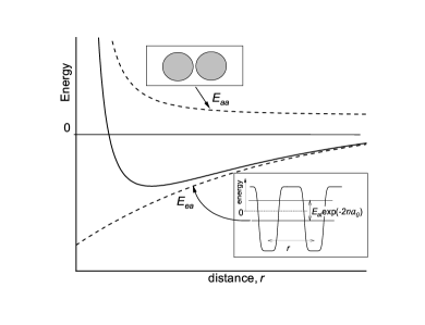
Figure 1: A qualitative form of potential energy of two atoms as a sum of repulsive core-to-core interaction due to the valence band formation.

Note that $E_{ea}$ originally represents the electronic energy vs. interatomic distance. Its time-average over the fast electronic movements (according to the adiabatic principle), is the potential energy of atomic nuclei. However, its electronic origin becomes important when we address the question of how the electronic energy will respond to changes in interatomic distance. As is seen in Fig. 1, $E_{ea}$ decreases when that distance becomes smaller, i. e. it is energetically favorable for the electrons to shorten a molecule. For example, adding one more electron with the same energy $E_{ea}$ will shift the balance (with $E_{aa}\rightarrow 2E_{aa}$) towards shorter lengths, thus shrinking the molecule. Such interactions between the electrons and atoms are commonly referred to as the deformation potential.

We mention here just one example of deformation potential responsible for sound absorption in metals. As is well known, a sound wave produces periodically distributed regions of higher and lower material density, which, through the deformation potential, trigger the electron redistribution towards denser regions where they have lower energies. The electric currents corresponding to such a redistribution will result in energy dissipation proportional to the metal resistivity; hence, the original energy of a sound wave transforming into Joule heat, which is sound absorption. We will go through a number of other examples of deformation potential interaction in Sec. IV.2 below.

In integral, our diatomic model is illustrated in Fig. 2. The characteristic linear and energy scales are given by $a_{0}\sim 2-3$ $\AA$ and $E_{at}\sim 3-5$ eV, as dictated by atomic physics. In what follows we accept for simplicity the rough order of magnitude estimates $a\sim 1$ $\AA$ and $E_{at}\sim 10$ eV. They are interrelated through $E_{at}\sim\hbar^{2}/(m_{e}a^{2})$, which interprets $E_{at}$ as the characteristic energy of the molecule binding electron localized in a linear domain of $a$.

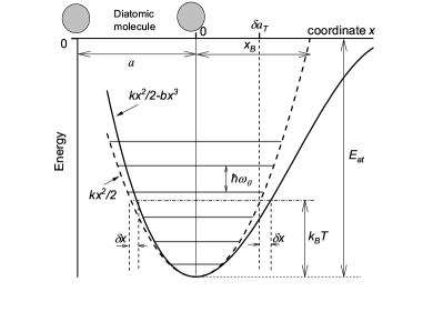
Figure 2: A sketch of potential energy and energy levels (not to scale) in a diatomic molecule presented with two circles in the top left corner. The dashed curve stands for the harmonic approximation. The horizontal domains represent the energy levels of a harmonic oscillator (separated by gaps of $\hbar\omega_{0}$), for definiteness chosen here to be significantly smaller than the characteristic thermal energy $k_{B}T$. $a$ is the equilibrium length of a molecule, $x_{B}$ is the elongation that would break it increasing $kx^{2}/2$ above the binding energy $E_{at}$ (note that the leftmost 0 in the figure corresponds to the energy axis). $\delta a_{T}$ is the amplitude of harmonic thermal vibrations, $\delta x$ is the change in that amplitude due to anharmonism.

II.1.1 Harmonic approximation

In the harmonic approximation, the potential energy of the molecule is $kx^{2}/2$ and the harmonic oscillation frequency is $\omega_{0}=\sqrt{k/M}$ where $M$ is the atomic mass (strictly speaking, the reduced atomic mass of the molecule, but that subtlety is not important here), which for the order of magnitude estimates we will take as $M\sim 10^{-22}$ g corresponding to the middle of the periodic table of elements. In harmonic approximation, the molecule breakup takes place at the characteristic stretch $x_{B}$ when $kx_{B}^{2}/2\sim E_{at}$ (see Fig. 2). Because we do not have any characteristic length at hand other than the atomic length $a$, we expect $x_{B}\sim a_{0}$, which yields, $k\sim E_{at}/a_{0}^{2}$, resulting in

$$\omega_{0}\sim 3\times 10^{13}\quad{\rm s}^{-1}\quad{\rm and}\quad\hbar\omega_{0}\sim 0.03\quad{\rm eV},$$ (1)

well within the ballpark of the accepted values for the frequencies and energies of atomic vibrations for both the molecules and condensed matter.

Note that the vibrational energy can be represented in the form,

$$\hbar\omega_{0}\sim E_{at}\sqrt{\frac{m_{e}}{M}}$$ (2)

where $m_{e}/M\ll 1$ ($m_{e}/M\sim 10^{-5}$ with parameters here) is the famous adiabatic ratio.

Furthermore, the characteristic vibration amplitude at zero temperature can be estimated as the De Broglie wavelength,

$$\delta a_{0}\sim\frac{\hbar}{p}\sim\frac{\hbar}{\sqrt{M\hbar\omega_{0}}}\sim a\left(\frac{m_{e}}{M}\right)^{1/4},$$ (3)

of the order of several percent of the characteristic atomic length.

In connection with the latter, we note the high temperature vibration amplitude $\delta a_{T}$ that increases with temperature $T$ (Fig. 2). For high enough temperatures $k_{B}T\gg\hbar\omega_{0}$ (where $k_{B}$ is the Boltzmann’s constant), the turning points condition yields, $k\delta a_{T}^{2}\sim k_{B}T$, and

$$\delta a_{T}\sim\sqrt{\frac{k_{B}T}{k}}\sim\sqrt{\frac{k_{B}T}{\hbar\omega_{0}}}\delta a_{0}.$$ (4)

When $\delta a_{T}$ increases above a certain fraction (typically 10 percent) of $a$, the material melts. This constitutes the well known (empirical) Lindeman criterion of melting. For our purposes, that criterion tells that the atomic vibration amplitudes are relatively small compared to the interatomic distances.

In the harmonic approximation, the diatomic model predicts that the internal energy equals the sum of averages of potential and kinetic energies, which are both equal to $k_{B}T/2$ in the classical limit $k_{B}T\gg\hbar\omega_{0}$ (equipartition theorem). The derivative of that energy versus $T$ gives the specific heat, $c=k_{B}$. For the low temperature quantum limit, $k_{B}T\ll\hbar\omega_{0}$, the probability of excitations from the ground level $\exp(-\hbar\omega_{0}/k_{B}T)$ becomes exponentially small, hence $c\rightarrow 0$. These predictions remain in the limiting cases of the Einstein solid model, that postulates equivalent harmonic vibration frequencies $\omega_{0}$ for all $N\gg 1$ atoms in a solid, predicting the heat capacitance

$$c=3Nk_{B}\left(\frac{\hbar\omega_{0}}{2k_{B}T}\right)^{2}\left[\sinh\left(\frac{\hbar\omega_{0}}{2k_{B}T}\right)\right]^{-2}$$ (5)

where the multiplier 3 reflects the fact that each atom can vibrate along three independent coordinates $x,y,z$. The exponentially small $c\propto\exp(-\hbar\omega_{0}/k_{B}T)$ predicted by Eq. (5) does not agree with the data, which reflects the inadequacy of the diatomic molecule model as explained below in Sec. III.

II.1.2 Anharmonic effects: thermal expansion

Based on the smallness of atomic vibration amplitudes, the potential energy of a diatomic molecule can be expanded beyond the harmonic approximation,

$$U(x)=kx^{2}/2-\beta x^{3}+...\quad{\rm with}\quad k\sim E_{at}/a^{2},\ \beta\sim E_{at}/a^{3}$$ (6)

where we have employed the estimate for $\beta$ combining the available parameters of needed dimensionality, along the lines of the above estimate for $k$. The negative sign in front of $\beta$ is taken on empirical grounds.

The difference between the harmonic and anharmonic approximation is illustrated in Fig. 2. It demonstrates the increase of the right and decrease of the left turning point coordinates determined by the condition $U(x_{T})=k_{B}T$; both changes are represented as $\delta x$ in $\delta a_{T}$ and a slight difference between them is neglected. We note now that in the harmonic approximation, the molecule vibrations are symmetric with respect to $x=0$ while the anharmonism makes the positive deformations larger in absolute values than the negative ones. The latter observation means that the average length of the molecule increases with temperature, thus representing thermal expansion.

The thermal expansion effect can be described more quantitatively by setting $U(\delta a_{T}+\delta x)=kT$ with $k\delta a_{T}^{2}/2=k_{B}T$ and $\delta x\ll\delta a_{T}$; here $\delta a_{T}$ is the high temperature amplitude of harmonic vibrations determined in Eq. (4). This yields the thermal expansion linear in temperature, $\delta x=2\beta k_{B}T/k^{2}$ with the thermal expansion coefficient

$$\alpha\equiv\frac{1}{a}\frac{d\delta x}{dT}=\frac{2k_{B}\beta}{k^{2}a}.$$ (7)

The thermal expansion is often described in terms of the dimensionless Grüneisen parameter $\Gamma=\alpha K/c$ where $K$ is the bulk modulus and $c$ is the thermal capacity. By definition, $2K$ is the proportionality coefficient between the square of dimensional dilation, $(\delta a_{T}/a)^{2}$ and the elastic deformation energy, i. e. $K\sim ka^{2}$. Taking into account the heat capacity $k_{B}$ and adopting the estimates for $k$ and $\beta$ from Eq. (6), one gets,

$$\Gamma\sim a\beta/k\sim 1,$$ (8)

in agreement with the data for high temperature Grüneisen parameters of the majority of solids.

We will come across other links with the concept of diatomic molecules later in the text, in Sections IV.1.1, IV.2, IV.2.3.

II.2 Two-level systems

Consider a system with two energy levels, 0 and $E$. They can represent the electron spin energies in magnetic field $H$ (in which case $E=2\mu H$ where $\mu$ is the Bohr magneton) or the energies of certain nonequivalent configurations (say, off-centers) of ions in some crystals, or other atomic configurations possessing multiple equilibrium points in amorphous solids or liquids. For specificity, we will assume here atomic-type excitations. A model of two local minima (double well potential) along some unspecified configurational coordinate is presented in Fig. 3. That particular model diagram presents two-level excitations with energies $E$ considerably lower than the intra-gap energy levels $\hbar\omega_{0}$, which is achieved due to low asymmetry $\Delta$ of two well minima and low tunneling splitting $V_{0}$.

It is interesting that the double well potential model often gives a good description, even for systems that have more than two local minima. That happens when the transitions between various pairs of wells (states) are practically independent or when efficient transitions take place within only one such pair. The latter may be a consequence of a relatively low height $W$ of their separating barrier. Apparently, such a situation takes place in amorphous systems where local atomic configurations are random and their significant differences make only one of them efficient. Indeed, the double well atomic potential has been established as one of the central concepts for glasses. The underlying physics is that glasses are obtained by freezing of a material from its melted state. A rapid freezing leaves some microscopic volumes of liquid material arrested by momentarily frozen surroundings. In those arrested micro-volumes, some atoms or groups of atoms retain their liquid-like motility, being able to move between several potential minima. Of all possible potential barriers, which are significantly different due to the system randomness, one is the lowest and its related inter-well transitions dominate; hence, double well potentials.

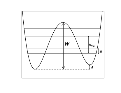
Figure 3: Sketch of a double well atomic potential with energy levels corresponding to two classical wells with energy minima difference $\Delta$ and the lowest energy level gap $E$; not to scale: should be $\Delta<E\ll\hbar\omega_{0}\ll W$.

A well known property of two-level systems is their contributions to the heat capacity $c(T)$ in the form of a peak at $T\approx E/k_{B}$ called the Schottky anomaly. Qualitatively, it can be understood by noting that for low $T\ll E/k_{B}$ the system cannot absorb any significant heat because there is not enough energy $kT$ to trigger upward transitions. In the opposite limit of $T\gg E/k_{B}$, both upper and lower energy levels are almost equally populated and practically no additional excitations are possible. Both the latter prohibitive factors are relaxed when $T\sim E/k_{B}$, where the specific heat must be at a maximum.

The same conclusion can be obtained more formally. For $N$ double well potentials, we use the definition $c=Nd\langle E\rangle/dT$ where $\langle E\rangle$ is the average energy per system. Using the standard definition of averages, $\langle E\rangle=0\times p_{0}+E\times p_{E}=E\times p_{E}$ where $p_{0}$ and $p_{E}$ are the probabilities of finding a system in a state with energy 0 and $E$ respectively. The Gibbs distribution of thermodynamics dictates that $p_{E}=p_{0}\exp(-E/k_{B}T)$. Substituting the latter in the condition of unit total probability, $p_{0}+p_{E}=1$, yields $p_{E}=[1+\exp(E/k_{B}T)]^{-1}$. Differentiating $\langle E\rangle=Ep_{E}$ gives the Schottky contribution to the heat capacity,

$$c_{S}=\frac{Nk_{B}\exp(E/k_{B}T)}{[1+\exp(E/k_{B}T)]^{2}}.$$ (9)

As a function of $T$,- it represents the Schottky anomaly, a peak in the vicinity of $T=E/k_{B}$, whose feature has been observed.

Furthermore, the double well potential model can include interaction between the two states by allowing quantum tunneling and its corresponding splitting $V_{0}$. Taking such splitting into account results in two states collectivized between the wells. The energy gap between them is given by,

$$E=\sqrt{\Delta^{2}+V_{0}^{2}}.$$ (10)

Eq. (10) follows from the perturbation theory for adjacent levels described in the Sec. A. The model of Eq. (10) with random $\Delta$ and $V_{0}$ describes a remarkably broad variety of phenomena in multiple glasses, such as specific heat, thermal conductivity, sound absorption, thermal expansion, etc. galperin1989

As a simple example, consider briefly the specific heat in glasses. Due to their inherent randomness, we accept that the energy gaps $E$ are random in the ensemble of double well potentials. If we concentrate on the low temperature properties with $k_{B}T\ll\hbar\omega_{0}$, then excitations with $E\ll\hbar\omega_{0}$ will dominate the observations. Because $E$ is much below any characteristic energies in a solid ($\hbar\omega_{0}$, $E_{at}$, etc.) there are no energy scales available to characterize their density of state $n(E)$ (DOS, number of states per energy pert volume) and we have to accept $n(E)=const$ for $E\ll\hbar\omega_{0}$. Therefore, the number of contributing states at temperature $T$ is estimated as $nk_{B}T$ and their related energy is $\langle E\rangle\sim kT\times(nk_{B}T)$. Differentiating the latter with respect to $T$ gives the low-temperature specific heat $c\sim nk_{B}^{2}T$. Of course, the same result could be obtained by integrating Eq. (54) over energies $E$. Such a specific heat -linear in $T$- was observed in a great number of glasses.

Our second example describes EM field absorption due to two-level systems illustrated in Fig. 4. In the absence of external perturbations, the fluctuations in the difference in populations of the bottom and top levels $\Delta n$ is described by the standard relaxation equation $d\Delta n/dt=-\Delta n/\tau$ where $\tau$ is the relaxation time. That equation guarantees that fluctuations decay with time exponentially, $\Delta n\propto\exp(-t/\tau)$. The absorption is due to the time delay between the events of particle excitation and relaxation as shown in Fig. 4. It is clear that when the frequency of oscillations is much higher than $1/\tau$, then very fast oscillations average out the absorption process. On the other hand, very slow oscillations allow the energy level populations to adiabatically follow their instantaneous positions; hence, suppressed dissipation. We arrive at the conclusion that dissipation must be a maximum at frequencies of the order of $1/\tau$.

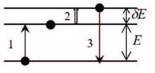
Figure 4: Mechanism of the relaxation absorption by a two level system. The energy gap $E$ is modulated by the external field with amplitude $\delta E\ll k_{B}T$ (fat arrow 2). The upward thermal transition of a particle takes place when the energy of the two-level system is close to its minimum value while the downward transition (3) occurs close to its maximum (3); hence the energy difference $\delta E$ dissipates into heat which is tantamount to absorption.

More formally, the external perturbation introduces the energy modulation with amplitude $\delta E\ll k_{B}T$ and frequency $\omega$ which translates into a stimulated modulation of the population difference $\delta E/k_{B}T$. The corresponding relaxation equation becomes

$$d\Delta n/dt=-\Delta n/\tau+(\delta E/k_{B}T)\exp(i\omega t).$$

Its solution takes the form of $\Delta n=\alpha\delta E\exp(i\omega t)$ with the susceptibility $\alpha=1/(1+i\omega t)$. The absorption coefficient is proportional to the imaginary part of the latter, i. e. $I\propto\omega\tau/[1+(\omega\tau)^{2}]$, a maximum at $\omega\tau\sim 1$. (More in detail derivation of the same is given by Kittel. kittelthin )

III Delocalized atomic vibrations: phonons and fractons

The atomic vibrations described in Sec. II.1 are confined to certain local entities such as diatomic molecules or double well atomic potentials. In condensed matter, each atom interacts with many others, all of them contributing to vibrations in a rather non-additive manner. In particular, we will see how the vibrational spectrum of an $N$-atomic linear chain is very different from the superposition of spectra of its constituting pairs of atoms.

More specifically, interactions of multiple coupled atoms make their vibrational excitations delocalized and spreading over the entire chain. Such excitations have a structure of waves, and quantization of such waves leads to the concept of phonons. Just like photons are the quanta of electromagnetic energy, phonons are the quanta of vibrational waves. The delocalized atomic vibrations in condensed matter exhibit two major modes: acoustic and optical (Fig. 5). In what follows, we neglect such additional features of acoustic and optical waves as their possible longitudinal or transverse nature displacements, as they do not have any significant effect on their qualitative properties.

We will start by considering the acoustic mode. In the acoustic mode the particles move coherently around their equilibrium positions such that there are places where the atoms are closer together and others where they are farther apart. (Fig. 5 (top) describes such squeeze - stretch motion for a system of identical atoms). This dynamic is similar to that of propagation of sound, which is the reason it is called acoustic. The angular frequency $\omega$ can be described by the standard concept of harmonic vibrations of a certain mass $M_{eff}$ attached to a spring of elasticity $k_{e}ff$:

$$\omega=\sqrt{\frac{k_{eff}}{M_{eff}}}.$$ (11)

where here, the effective spring constant mass will depend on the vibration wavelength.

Consider elastic waves of wavelength $\lambda$ (and wavenumber $q$) in a linear chain with interatomic distance $a$ as in Fig. 5 (top),

$$\lambda=Na\quad{\rm and}\quad q\sim 1/\lambda.$$ (12)

Here $N$ is the number of atoms per wavelength. A $\lambda$-domain dilation $\delta x$ translates into $\delta x/N$ per individual interatomic bond; hence the force and effective spring constant are smaller by the factor of $N$,

$$k_{eff}=\frac{k}{N}.$$

The effective mass of atoms taking part in such vibrations is

$$M_{eff}=MN.$$

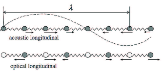
Figure 5: Atomic displacements for acoustic (top) and optical (bottom) vibrations

Figure 6: Qualitatively predicted (left) and realistic (right) phonon dispersion curves.

Substituting these estimates into Eq. (11) and taking into account Eq. (12) yields the dispersion law (see Fig. 6)

$$\omega=vq\quad{\rm with}\quad v=a\omega_{0}\quad{\rm and}\quad\omega_{0}=\sqrt{k/M}$$ (13)

Here $v$ has the meaning of sound velocity. Using the numerical values from Sec. II.1 we estimate $v\sim 3\cdot 10^{5}$ cm/s, in the ballpark of data for a variety of solids. Also, we note that the minimum wavelength should be set equal to the interatomic distance, $\lambda_{min}=a$. This corresponds to, $q\leq q_{max}\sim 1/a$ in Eq. (13) (Note that we neglect numerical coefficients such as $2\pi$ in $q=2\pi/\lambda$.)

In the case of optical vibrations, the non-identical nearest neighbor atoms move in pairs oscillating about their center of mass (bottom chain in figure (Fig. 5). These vibrations with non-identical atoms bearing non-equivalent electric charges form oscillating electric dipoles capable of interacting with electromagnetic fields; hence, the name of optical phonons; they are responsible for light scattering and other optical phenomena in solids. For optical vibrations, one gets

$$k_{eff}=Nk,$$

because the deformation of $N$ springs will take place simultaneously. The mass remains the same as in the previous case, $M_{eff}=MN$. Substituting this again into Eq. (11) gives,

$$\omega=\omega_{0}=const(q).$$ (14)

The above presented phonon dispersion laws are in qualitative agreement with the measured curves (Fig. 6). The deviations in the region of $\lambda\sim a$ are due to strong interference between the propagating waves and their reflections from atoms. Such reflections create standing waves whose zero group velocities, $d\omega/dq=0$ correspond to flattening of the dispersion curves at $q\rightarrow q_{max}$.

Looking at the same from a different angle, migdal we note that since the system does not dissipate energy, it must remain invariant under time reversal ($t\rightarrow-t$). Therefore, the equation determining its frequency spectra can contain only even powers of $\omega$. [For example, the Fourier transform of Newton’s law for small vibrations, $M\ddot{u}_{n}=-\sum_{m}F_{mn}u_{m}$ becomes $M\omega^{2}\tilde{u_{n}}=\sum_{m}F_{mn}\tilde{u_{m}}$.] Consequently, it is $\omega^{2}$ (and not just $\omega$) that must be an analytical function of the system parameters. In particular, for small wave-vectors,

$$\omega^{2}=a+v^{2}q^{2}+bq^{4}+...$$

For sound waves, the limit $q\rightarrow 0$ corresponds to the displacement of a system as a whole that does not change its energy; hence, $a=0$ and $\omega=vq$. For optical vibrations, there is no reason to nullify $a$; hence, $\omega=\sqrt{a}=const$ when $q\rightarrow 0$.

III.1 Phonon density of states

Similar to photons, phonons exhibit both particle and wave properties. Each phonon is characterized by its energy $E=\hbar\omega$ and momentum $p=\hbar q$ related through the dispersion law $\omega(q)$. The phonon density of states (DOS) $D(\omega)$ is defined as a number of phonon states per unit frequency interval in the proximity of a given frequency, $D(\omega)=dN(\omega)/d\omega$. The concept of phonon DOS plays an important role with multiple applications ranging from the thermodynamic to interactions of atomic vibrations with radiation and electrons.

For acoustic phonons, the number of states with frequencies below $\omega$ can be counted by noting that they are the same as the states with momenta below $p(\omega)$. The corresponding phase volume, and thus the number of states is proportional to $p^{3}$, the volume of a sphere of radius $p$ in the momentum space. Because $\omega\propto p$, (Eq. (13))this gives $N(\omega)\propto\omega^{3}$ and $D(\omega)\propto\omega^{2}$.

The proportionality coefficient in the latter relation will depend on the volume of the system and can be readily estimated from its dimensionality. For example, DOS per atom will have the dimension $\omega^{-1}$. Having only the characteristic frequency ($\omega_{0}$) at hand, the choice becomes:

$$D(\omega)\sim\frac{\omega^{2}}{\omega_{0}^{3}}.$$

This formula can be easily generalized to the case of arbitrary dimensions $d=1,2,3,..$,

$$D(\omega)\sim\frac{\omega^{d-1}}{\omega_{0}^{d}}.$$ (15)

Strictly speaking, the coefficient in the latter relations should be corrected to preserve the number of degrees of freedom per atom, which was originally 3 (before the atom is made a part of a solid). Therefore we require

$$\int D(\omega)d\omega=3.$$

To maintain the latter relationship, the upper limit in the integral is chosen to be somewhat different from $\omega_{0}$. Namely, it should be defined as the Debye frequency,

$$\omega_{D}=(3d)^{1/d}\omega_{0}.$$ (16)

As a result

$$D(\omega)=\frac{\omega^{d-1}}{\omega_{D}^{d}},\quad\int_{0}^{\omega_{D}}D(\omega)d\omega=3.$$ (17)

In most practical applications, however, the difference between $\omega_{D}$ and $\omega_{0}$ is insignificant.

For the case of optical phonons, the dispersion is not very significant, DOS is large in a limited energy interval and can be approximated by the delta-function,

$$D(\omega)\sim\delta(\omega-\omega_{0}).$$

The proportionality coefficient depends on the microscopic structure of a primitive cell that may have several atoms giving rise to different types of phonon polarization.

III.2 Specific heat

By definition, the specific heat of a system is given by:

$$C=\frac{dU}{dT}$$

where $U$ is the system energy. Phonons are traditionally treated with Bose-Einstein statistics where the number of phonons $dN=n\hbar d\omega$ with energy in the interval $\hbar d\omega$ has is described through the occupation number $n(\hbar\omega)=1/(\exp(\hbar\omega/k_{B}T)-1)$. In particular, the energy $U$ can be evaluated by integration of the product $n(\hbar\omega)D(\omega)$ over all phonon frequencies.

We now present a simpler argument for the evaluation of phonon specific heat. At low temperatures, such that $k_{B}T\ll\hbar\omega_{0}$, one gets $n(\hbar\omega_{0})\sim\exp(-(\hbar\omega_{0}/k_{B}T))\ll 1$. Therefore the probability of optical excitations and their contributions to $U$ are negligibly small, and we can take into account only acoustic phonons. Their energy is estimated as the number of active phonon states $N$ with energies $\hbar\omega_{0}\lesssim k_{B}T$ times the thermal energy $k_{B}T$,

$$U\sim kTN(\omega=k_{B}T/\hbar)\sim k_{B}T\frac{(kT)^{d}}{(\hbar\omega_{0})^{d}}.$$ (18)

Therefore,

$$C\sim k_{B}\left(\frac{T}{T_{D}}\right)^{d}\quad{\rm where}\quad T_{D}=\frac{\hbar\omega_{D}}{k_{B}}$$ (19)

and $T_{D}$ is known as the Debye temperature.ashcroft

As the temperature increases towards $T_{D}$, all the available states become affected, their number saturates, and so does the specific heat.

III.3 Thermal expansion and Grüneisen parameter

So far we used the harmonic oscillator (quadratic) potential for phonons. It was demonstrated in Sec. II.1 how the anharmonicity in local vibrations can be responsible for thermal expansion. The thermal expansion coefficient

$$\alpha=\frac{1}{V}\frac{dV}{dT}$$

can be used in the dimensionless Grüneisen parameter,

$$\Gamma=K\frac{\alpha}{C}$$

where the bulk modulus $B$ is defined as the fractional change in volume $\delta V/V$ produced by a change $\delta p$ in pressure.

$$K=-\frac{\delta p}{\delta V/V}.$$

The Grüneisen’s law states that $\Gamma$ is temperature independent. To show this we write the change in the potential energy due to the deformation as

$$\delta U=K\left(\frac{\delta V}{V}\right)^{2}-(d)(k_{B}T)\frac{(kT)^{d}}{(\hbar\omega_{0})^{d+1}}\frac{\partial\hbar\omega_{0}}{\partial V}\delta V$$

where $(d)$ is the system dimensionality. Here the first and second terms represent respectively the change in energy of a deformed isotropic body landauelast and the change in the phonon energy $U$ from Eq. (18). The latter is attributed to the change in characteristic frequency $\omega_{0}$. Direct minimization with respect to $\delta V/V$ gives

$$\frac{\delta V}{V}=\frac{d}{2K}\left(\frac{T}{T_{D}}\right)^{d+1}\frac{\partial\hbar\omega_{0}}{\partial V}V.$$

Estimating here $|\partial\hbar\omega_{0}/\partial V|\sim\hbar\omega_{0}/V$ yields

$$\left|\frac{\partial\delta V}{\partial T}\right|\sim\frac{1}{K}C$$

where $C$ is the specific heat from Eq. (19). Finally we arrive at $|\Gamma|\sim 1$ in agreement with the majority of data for different solids and with a more naive estimate in Sec. II.1.

Note that in the above derivation, the effect of anharmonicity was implicitly taken into account by assuming the limiting frequency $\omega_{0}$ dependent on deformation. Note also that while $|\alpha|\sim 1$, the sign of $\alpha$ remains arbitrary. Indeed, it varies between different solids.

III.4 Vibrations on fractals. Fractons

Fractal networks can describe a variety of random (but not necessarily only random) polymer-like systems illustrated in Fig. 7. For such objects, the mass confined in a volume of linear dimension $R$ is proportional to $R^{\overline{d}}$ where $\overline{d}$ is called the principal (or Hausdorff)mandelbrot fractal dimension. The architecture of tree branches can give a simple example of the latter mass scaling when the linear size $R$ is shorter than the linear size of a tree.

As a first intuitive assessment, it is obvious that elastic waves on fractals will be considerably different from that in a continuous medium. Indeed, a fractal contains many pieces of one-dimensional architecture, for which DOS $\propto\omega^{d-1}=const$, hence, the specific heat $C\propto T$. Because these pieces are connected in the higher dimensionality objects, one can expect a composite DOS $\propto\omega^{d-1}$ with $d$ in between 1 and 3.

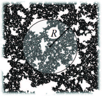
Figure 7: A fractal structure representing polymers or composite materials. A semitransparent circle of radius $R$ encompasses the diffusion range over a certain time or that of vibration of certain frequency.

It is not immediately clear though, how to describe elastic waves in fractals. In particular, the simplest (isotropic) form of the elastic wave equation

$$\rho\ddot{u}=K\nabla^{2}u$$ (20)

where $u$ is the displacement and $\rho$ is the mass density, contains the Laplacian $\nabla^{2}$, which is the sum of second derivatives. It is hard to imagine how to define the second (or even the first) derivative for the case of an irregular structure.

The following consideration shows how to treat the Laplacian on an intuitive basis (although the question of derivatives in fractals has been addressed by pure mathematics). The approach below draws a plausible analogy with the diffusion equation that is also based on the Laplacian,

$$\dot{n}=D\nabla^{2}n$$ (21)

where $n$ is the concentration and $D$ is the diffusion coefficient. This diffusion problem in a fractal known also as the “ant in the labyrinth” has been solved by numerical modeling for many different fractals. The main result of it is that the diffusion is slower than that of regular lattices, which is natural due to the presence of dead ends, closed loops, etc.

The latter slowness is described by the diffusion coefficient

$$D\propto R^{-\theta}$$ (22)

where $\theta$ is the diffusion fractal index. We also note that the Eq. (22) can be written as

$$\frac{\partial\eta}{\partial(Dt)}=\nabla^{2}\eta.$$

Approximating $\partial n/\partial(Dt)\sim n/Dt$ and $\nabla^{2}\sim 1/R^{2}$, leads to the standard relation $Dt\sim R^{2}$. As a result, the characteristic distance $R$ for propagation of a packet varies with time as

$$R\propto\sqrt{Dt}\propto t^{1/(2+\theta)}.$$ (23)

We now note the difference in the time derivatives in the vibrational ($\ddot{u}$) and diffusion ($\dot{u}$) equations. The time Fourier transforms will then generate the frequency powers $\omega^{2}$ and $\omega$ in these equations respectively. Replacing $t\sim\omega^{-1}$ in Eq. (23) and then replacing $\omega$ with $\omega^{2}$ (to switch from diffusion to vibrations) gives

$$R\propto\omega^{-2/(2+\theta)}.$$ (24)

This gives the relationship between the linear dimension of a vibrational state and its frequency. To normalize this quantity to the number of vibrations per atom, we note that the number of states per atom is proportional to $R^{-\overline{d}}\propto\omega^{2\overline{d}/(2+\theta)}$. Finally DOS is given by

$$D(\omega)\propto\frac{d}{d\omega}\omega^{2\overline{d}/(2+\theta)}\propto\omega^{\overline{\overline{d}}-1}$$ (25)

where

$$\overline{\overline{d}}=\frac{2\overline{d}}{2+\theta}$$

is called the fracton dimension. According to Alexander and Orbach alexander , $\overline{\overline{d}}\approx 4/3$ for a wide class of different fractal structures (in spite of the fact that $\theta$ and $\overline{d}$ vary considerably between different fractals in that class). This kind of DOS and related heat capacity were indeed observed in polymers. We note as well that the diffusion on fractals and fracton dimensionality describe the alternating current conduction on percolating clusters. schroder2008

IV Electronic properties

IV.1 Band structure

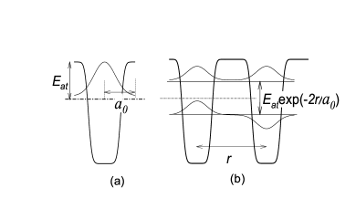
Figure 8: Electron energy splitting in a system of two identical potential wells separated by distance $r$. Curved lines represent the wave functions. $a_{0}$ is the decay length of a wave function for a single atom.

The energy levels of electrons in crystals form finite width continuous bands separated by empty (forbidden) gaps. That energy structure can be described based on two different premises: (a) local basis approach where the bands are interpreted as the significantly broadened energy levels of the material’s constituting atoms with the broadening caused by interatomic interactions, and (b) extended basis approach starting with the continuum of extended electron states fully collectivized between the constituting atoms, with boundaries caused by interference effects in a periodic atomic structure. We consider both the approaches.

IV.1.1 Local basis

As a thought experiment, we can form a material by first combining its constituting atoms in pairs, then forming pairs of pairs, pairs of pairs of pairs, etc. For specificity, we assume atoms with ionization energy $E_{at}\sim 10$ eV and electron radius $a_{0}\sim 1$ Å(Fig. 8). As our first step we note that when two identical atoms form diatomic molecules their electronic states combine to form the bonding and antibonding orbitals separated by the energy gap

$$G=E_{at}\exp(-2r/a_{0})$$ (26)

For the typical interatomic distances $r\sim 2$ Å, their energy spectrum consists of a pair of energy levels separated by the gap $G\sim 1$ eV. Combining two diatomic molecules will introduce another splitting, and so on, as shown in the diagram of Fig. 9. This can result in either two bands separated by the gap $\sim G$, or in the overlapping bands with no gap in between. Alternatively, the bands could originate from the different atomic levels. This may change certain band properties, but typically will not affect the order of magnitude estimates here.

Figure 9: Band formation as a consequence of the pairing energy splitting .

Within the band, the electron has the quasi-continuous spectrum with delocalized wave functions characterized by the momentum $p=\hbar k$. The wave number $k$ varies between zero and the maximum value $k_{max}\sim 1/a$, where $a$ is the lattice parameter (interatomic distance) for the case under consideration. $k_{max}$ corresponds to the shortest possible wavelength $\lambda_{min}\sim a$.

Close to the band edge ($E_{0}$) we can express the electron energy as

$$E=E_{0}+b_{2}k^{2}+b_{3}k^{3}+b_{4}k^{4}+...$$

where $k\ll k_{max}$. Retaining only the quadratic term and setting $E_{0}=0$ enables one to present

$$b_{2}\sim\frac{\hbar^{2}}{m^{*}}$$

where $m^{*}$ has the dimension of mass and is called the effective mass. Because the only available quantity of the right dimension is the electron mass, one can expect

$$m^{*}\sim m.$$

While generally true, the latter estimate can miss significant numerical factors, so effective masses can be quite different, say $m^{*}\sim(0.1-0.3)\cdot m$. In some cases $m^{*}$ can be significantly larger than $m$.

There is a simple approximate relationship between $m^{*}$ and the band width $B$. Namely, if we extend the quadratic approximation

$$E-E_{0}=h^{2}k^{2}/2m^{*}$$

throughout the entire band by setting $k\sim k_{max}\sim 1/a$, then

$$B\sim\frac{\hbar^{2}}{m^{*}a^{2}}.$$ (27)

The latter relationship, however approximate, adequately reflects the trend: narrow band materials have large effective masses, while wide band materials have light $m^{*}$.sze

We shall end this subsection by noting that the energy gap $G=E_{at}\exp(-2r/a_{0})$ will change with the system’s deformations increasing or decreasing with interatomic distances $r$. That mechanism of deformation-induced variations in electronic energies is often called deformation potential. As such, it was present already in the earlier Fig. 2 where the increasing (right to the minimum) part of the energy can be associated with the bonding orbital energy, $E_{at}\exp(-2r/a_{0})$. The deformation potential concept will be extensively used in Sec. IV.2.

IV.1.2 Extended basis

In the extended basis model, the electron states extend over all the atoms in a material. In the first approximation, they are described as plain waves $\psi=\exp(i{\bf kr})$ characterized by certain wave vectors ${\bf k}$ and their corresponding energies $E(k)=\hbar^{2}k^{2}/2m$. These plain waves are affected by the presence of the lattice. We consider the lattice potential as a perturbation.

When the lattice is present, the wavefunction should not change under the translation ${\bf r}\rightarrow{\bf r+a}$ where ${\bf a}$ is the vector of lattice translation. To reflect that translational invariance, the wave vector should change by kittel $\delta{\bf k}={\bf g}$, where $\bf g$ is called the vector of the reciprocal lattice; its absolute value is $(2\pi/a)$. Therefore the description of electron energies will not change if we translate the original dispersion parabola $E(k)=\hbar^{2}k^{2}/2m$ by ${\bf g}$ as shown in Fig. 10.

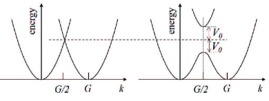
Figure 10: Forbidden zone formation due to the repulsion of degenerate electronic terms.

Fig. 10 (left) shows the dispersion curves shifted relative to each other by the wave vector ${\bf g}$. The degeneracy of the states belonging to these dispersion curves at the point of their intersection, ${\bf k=g/2}$ can be eliminated by small perturbations physically produced by a lattice. The corresponding perturbation theory for degenerate states landauqm ; migdal predicts that the two curves will repel forming a gap $G$ in the energy spectrum.

More specifically the degenerate perturbation theory is described by Eq. (58) in the appendix A. Denoting the unperturbed energies by

$$E_{(g/2)\pm\delta}=\frac{\hbar^{2}}{2m}\left(\frac{\pi}{a}\pm\delta\right)^{2}$$ (28)

close to the intersection point ${\bf k}={\bf g}/2$, the perturbed energies take the form

$$E_{\pm}(\delta)=\pm\sqrt{\left(\frac{E_{(g/2)+\delta}^{0}-E_{(g/2)-\delta}^{0}}{2}\right)^{2}+V_{0}^{2}}$$ (29)

where $\delta$ is a wavenumber measured from the intersection point.

The gap in the spectrum is $2V_{0}$. Furthermore, close to the intersection point, $\delta\ll g/2$, one can reduce the square root in Eq. (29) to the form

$$\pm\left(V_{0}+\frac{4\pi^{2}\hbar^{4}\delta^{2}}{m^{2}a^{2}V_{0}}\right)\equiv\pm\left(V_{0}+\frac{\hbar^{2}\delta^{2}}{2m^{*}}\right)$$ (30)

where the effective mass is given by

$$m^{*}=m\frac{V_{0}}{4\pi^{2}\hbar^{2}/ma^{2}}\sim m\frac{G}{B}.$$

Note that $m^{*}$ again has a negative correlation with the band width, which in this case appears as $B=8\pi^{2}\hbar^{2}/ma^{2}$.

As a general note, it is due to the dimensionless factor of $G/B$ that the ratio $m^{*}/m$ cannot be estimated with more certainty: any dependence of the type $m^{*}=mf(G/B)$ where $f$ is a ‘reasonable’ (but arbitrary) function remains a possibility.

Also, we note that approximating the quadratic dispersion curve of Eq. (30) over the entire allowed region $0<\delta<\pi/a$ results in the estimate for the allowed energy band $B=\pi^{2}\hbar^{2}/(m^{*}a^{2})$, which is consistent with the alternative approach estimate in Eq. (27).

IV.2 Electron-phonon interaction

We have so far considered conduction electrons that move through a lattice whose atoms are frozen in place. In reality, a moving electron does interact with the ion cores; in an oversimplified picture, the electron pulls nearby positive ions and pushes negative ions away. Even if there are no “real” phonons present, the electron will still interact with zero-point lattice vibrations. According to the previous section (particularly, Eq. (26)), the energy $E$ of the electron at the bottom of a conduction band (or the hole at the top of the valence band) will depend on the interatomic distance $r$. If we assume that the interaction is rather weak, and only retain the linear term in the expansion of the exponential in equation (26), then we can write $\delta E\sim B\delta r/a$. Introducing here the dimensionless dilation $u\equiv\delta r/a$, gives

$$\delta E=Qu.$$ (31)

The proportionality coefficient $Q$ between the electron energy and the dilation is known as the deformation potential. Note that the latter linearization could be equally applied to the rising part of potential energy in Fig. 2. Therefore all the consideration addressing electron-phonon interactions below will qualitatively apply not only to solids but to molecules as well, showing again their representativeness of condensed matter physics.

A more realistic description would distinguish between different types of deformation (and introduce the corresponding deformation potential tensor $Q_{ij}$ as a matrix of coefficients between the $i$th component of deformation and the energy of the electron moving along the $j$th axis). Neglecting this anisotropy we roughly estimate a scalar $Q\sim B$, that is $Q$ of the order of several eV.

The above deformation effect is referred to as the electron-phonon interaction. Indeed, each phonon can be considered as a source of deformation that can change the electron energy. Along these lines, any arbitrary deformation can be represented as a superposition of partial deformations related to a (complete) set of phonons. In other words, the deformation potential, is a Hamiltonian of the electron-phonon interaction that can be used to describe the electron-phonon scattering.

IV.2.1 Polaron effect

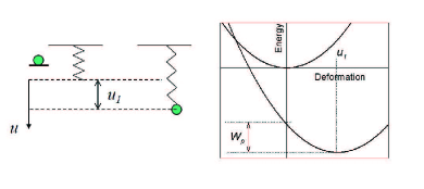
Figure 11: Left: Deformation of a spring with a hanging particle as a model for the electron-lattice interaction. Right: Energy vs. deformation for the case when the electron is not present (upper parabola), and in the presence of the electron.

One consequence of the deformation potential interaction is the polaron effect.landaupekar We will start with noting that the linear deformation interaction $Qu$, takes place in parallel with the quadratic increases in elastic energy, $\kappa u^{2}/2$, as stated by Hook’s law, where $\kappa$ is the elastic modulus. Therefore the total energy of our system (electron and lattice),

$$W=E_{0}-Qu+\frac{\kappa u^{2}}{2}$$ (32)

becomes formally equivalent to that of a particle of mass $m$ hanging on a spring in a uniform gravitational field. In this latter case $Q=mg$ and $u$ is the spring elongation. This analogy extends rather far. Similar to the equilibrium spring elongation, one can find the stationary ($dW/du=0$) material deformation $u_{1}$ that minimizes the system energy:

$$u_{1}=\frac{Q}{\kappa}\quad{\rm and}\quad W_{min}=E_{0}-\frac{Q^{2}}{2k}\equiv E_{0}-W_{p}$$ (33)

where $W_{p}$ is called the polaron shift (Fig. 11). Here, $E_{0}$ is the electron energy in the system prior to the deformation. For example, $E_{0}$ is the energy of the electron at the bottom of the conduction band, or it can be the energy of the electron localized at a defect state (located inside the energy gap) before the deformation occurred. Note that while the system energy changes by $W_{p}$, the electron energy change is twice as large,

$$E_{0}-Qu_{1}=E_{0}-2W_{p}.$$ (34)

From this consideration we conclude that it may be energetically favorable for the system to create a local deformation thus decreasing the electron energy. However, the parameters $Q$ and $\kappa$ in the above consideration are not strictly defined; for example, they appear unrelated to a particular type of the electron wave function, localized or delocalized, number of electrons involved, their kinetic energies, spin states, etc.

IV.2.2 Negative-$U$ centers

To be more specific, we will next consider the electron states localized at some defects. In that case, the electron wave function has a finite size, typically of the order of the corresponding de Broglie wavelength, $R\sim\hbar/\sqrt{m^{*}E}\sim 10\AA$ where $E\lesssim G$ is the defect binding energy, $G\sim 1-2$ eV is the forbidden gap, and $m^{*}\sim(0.1-0.5)m$ is the effective mass. We assume that $Q\sim 1-2$ eV remains a good estimate for the deformation potential, and will use $k\sim 3-5$ eV for the elastic modulus (same order of magnitude as the ionization energy). The corresponding polaron shift is

$$W_{p}\sim 0.1-1\quad{\rm eV}.$$

With these figures in mind, we consider the possibility of the two electrons pairing at the same defect center. This phenomenon is called the negative Hubbard energy (or negative correlation energy, or negative $U$)hubbard ; anderson and does take place in a variety of materials, specifically in chalcogenide glasses, some of A²B⁶ semiconductors, and possibly in superconducting ceramics. Its essence is that instead of one electron occupying each defect center, the electrons prefer to form pairs (of opposite spins) filling one half of such centers while leaving the other half empty; the singly occupied electron states appear energetically unfavorable.

The pairing mechanism is illustrated in Fig. 12, starting with the analogy of two point masses hanging on elastic springs. Using classical mechanics, we can see that the energy of the two individual masses, each hanging on one spring is higher than the energy of the two masses hanging together on the same spring. In our case at hand, the pairing energy gain can be estimated based on the approach similar to that in Eq. (32),

$$W_{n}=nE_{0}-nQu+\frac{\kappa u^{2}}{2}+U_{c}\delta_{n,2}.$$ (35)

Here $n=0,1,2$ is the center (spring) occupation number and $U_{c}$ is the Coulomb repulsion that takes place when $n=2$. In the simplest approximation,

$$U_{c}\sim\frac{e^{2}}{\varepsilon R}\sim 0.2\quad{\rm eV}$$

assuming the dielectric permittivity $\varepsilon\sim 10$.

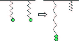
Figure 12: Mechanism of electron pairing represented in terms of elastic springs.

Optimizing Eq. (35) yields the equilibrium energies,

$$W_{n,min}=nE_{0}-n^{2}W_{p}+U_{c}\delta_{n,2}.$$ (36)

The correlation energy is defined as the difference between the state of a pair of electrons and that of the two separate electrons,

$$U=W_{2,min}-2W_{1,min}=-2W_{p}+U_{c}.$$ (37)

With the above estimates for $W_{p}$ and $U_{c}$ in mind, both the cases of $U<0$ and $U>0$ become possible, depending on particular values of the material parameters. Softer materials with small $\epsilon$ (glasses, polymers) and locally soft configurations (locally soft atomic potentials due to special defect structure configuration or random softening in disordered materials such as chalcogenide glasses) are especially likely candidates for the negative-$U$ phenomenon. The latter entails numerical consequences, such as the diamagnetism coexisting with a finite electron density at the Fermi level, abnormally large difference between the characteristic energies of absorption and photoluminescence (PL), and some others.

IV.2.3 Electron transition energies

In the case of a considerable polaron effect, the same electron state is characterized by considerably different energies corresponding to its (1) thermal ionization ($E_{T}$), (2) photo-ionization ($E_{PI}$) and (3) PL ($E_{PL}$). The nature of these differences is illustrated in Fig. 13.

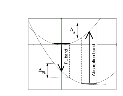
Figure 13: Absorption and PL transitions associated with defect state in a deformable medium.

The absorption process is depicted by an upward arrow from the state of the most likely (equilibrium) deformation of the bottom parabola. If we assume that the deformation does not change, the u coordinate will remain unchanged in the course of the transition, and the arrow from the bottom to the top parabola will be almost vertical. This is consistent with the standard adiabatic approximation: the electron transitions are so fast that the atomic nuclei do not have time to follow. (The optical transition time corresponding to a $600$ nm wavelength is of the order of $10^{-15}$ s). Similarly, the PL transition is depicted by the downward arrow; its energy is noticeably lower than that of the absorption. The thermal ionization energy is, by definition, the minimum work we need to perform in order to take the electron from the center. (This minimality does not rule out the non-adiabatic transitions.) As a result, $E_{T}$ is given by the energy difference between the two parabola minima. Photo-ionization on the other hand, is the photo-induced decrease of the charge of the system by one electron. In our case, the upper parabola corresponds to the energy of the system without one electron, while the bottom parabola corresponds to the energy of the system with the electron. To calculate the length of the photo-ionization arrow, we have to first traverse the energy $E_{T}$ (from the bottom minimum to the top minimum) and them add the energy $1/2\kappa u_{1}^{2}$ that will bring us to the top parabola. Since $u_{1}=Q/\kappa$ and $W_{p}=Q^{2}/2\kappa$, we can see that

$$E_{PI}=E_{T}+\frac{1}{2}u_{1}^{2}=E_{T}+W_{p}$$

From Fig. (13) we see that $E_{T}=E_{PL}+W_{0}$, therefore

$$E_{PL}+2W_{p}.$$

The polaron shift can be estimated as a half difference between the centers of the absorption and PL bands as shown in (Fig. 14).

Figure 14: Absorption and PL bands corresponding to the transitions shown in Fig. 13.

To estimate the PL and absorption bands, we note that the system is not strictly localized at the parabolic minimum but it is rather exercising small vibrations with characteristic amplitude $\lambda$. For low temperatures, ($k_{B}T\ll\hbar\omega$) $\lambda$ can be estimated using the zero-point energy of the harmonic oscillator $E=\hbar\omega$. From the De Broglie wavelength $\lambda=\hbar/p$ we can obtain:

$$\lambda=\sqrt{\frac{\hbar}{M\omega}}$$

For high temperatures ($k_{B}T\gg\hbar\omega$), we can estimate $\lambda$ using the energy of the harmonic oscillator: $k_{B}T\sim 1/2k\lambda^{2}$ which gives us:

$$\lambda\sim\sqrt{\frac{2k_{B}T}{\kappa}}$$

In both cases $M$ is the characteristic atomic mass and $\omega$ is the characteristic frequency of atomic vibrations.

We will now estimate the width of the absorption and PL bands, which according to figure (13) are approximately equal for small deformations. Considering a small change in the energy of the harmonic oscillator near the point $u_{1}$ gives us

$$\Delta_{PL}\sim\Delta_{a}\sim\frac{1}{2}u_{1}^{2}-\frac{1}{2}(u_{1}-\lambda)^{2}=\kappa\lambda u_{1}=\lambda Q=\frac{\lambda}{u_{1}}W_{p}$$

We note that generally $\lambda/u_{1}$ is much less than unity, because $u_{1}$ can be comparable to the atomic length, while the atomic vibration amplitude $\lambda$ is considerably smaller, say $\lambda/u_{1}\sim 0.1-0.3$.

IV.2.4 Multi-phonon electron transitions

Consider the probability of the electron downward transition between two energy levels separated by the energy gap $\Delta E\gg\hbar\omega$. It is proportional to the probability $p_{N}=p_{1}^{N}$ of emitting

$$N_{ph}=\frac{\Delta E}{\hbar\omega}$$

phonons needed to dissipate the energy. The latter probability can be equally represented in the form

$$p_{N}=\exp\left(-\gamma\frac{\Delta E}{\hbar\omega}\right),\quad\gamma\equiv\ln\left(\frac{1}{p_{1}}\right)$$ (38)

common to many other adiabatic electron transition probabilities (such as e. g. multi-photon ionization of atoms).

In the physics of semiconductors, one of the most important applications of the energy dependence in Eq. (38) is that the energy levels in the middle of the forbidden gap ($\Delta E\sim G/2$) appear the most efficient recombination centers as is generally accepted on empirical grounds. Eq. (38) does predict that the energy $G/2$ optimizes between the probabilities of an electron going downward to the defect level $\Delta E_{1}\sim G/2$) and then further downward ($\Delta E_{2}\sim G-\Delta E_{1}\sim G/2$) to recombine with a hole in a valence band. It is illustrated in Fig. 15

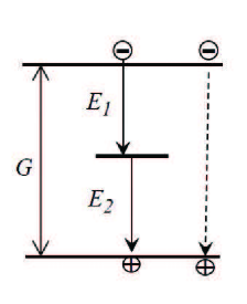
Figure 15: Electron-hole recombination through a midgap defect level vs the direct, without defect recombination with exponentially lower probability $\sim\exp(-\gamma G/\hbar\omega)$ deformation.

The above reasoning leading to Eq. (38) can be somewhat deceptive, since in a deformable medium the required change in the electron energy can be significantly different from that of the system energy due to the electron-lattice interaction. As is illustrated in Fig. 16 the transition probability can be more accurately related to overcoming the potential barrier formed by a point of intersection between the initial and final electron states in a deformable medium. mott ; baran1986 Omitting the details, that barrier can either decrease or increase with $\Delta E$, depending on the relationship of $\Delta E$ and the energy $2W_{p}$ representing the difference between the energy of bare (before deformation) and equilibrium electron energy. In particular, when $2W_{p}>\Delta E$, the corresponding transition probability

$$p\propto\exp\left(-\gamma\frac{2W_{p}-\Delta E}{\hbar\omega}\right)\propto\exp\left(\gamma\frac{\Delta E}{\hbar\omega}\right)$$

increases with $\Delta E$. On the contrary, for the case of $2W_{p}<\Delta E$ the original dependence in Eq. (38) takes place. In terms of parameters, both cases are possible and can give rise to a number of observed phenomena.

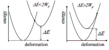
Figure 16: Electron transitions for the cases of $\Delta E>2W_{p}$ and $\Delta E<2W_{p}$ shown in the electron energy level diagram and the corresponding electron terms vs. system deformation.

IV.2.5 Small polaron collapse

Consider a polaron in the ideal crystal.chat2018 Its energy is given by the expression that generalized the above analysis to include the electron wave function $\psi({\bf r})$,

$$W=\frac{\hbar^{2}}{2m}\int(\nabla\psi)^{2}d^{3}r-Q\int u\psi^{2}d^{3}r+\frac{k}{2}\int u^{2}d^{3}r.$$ (39)

Here the first term describes the electron kinetic energy, the second one stands for the deformation potential interaction, and the last term accounts for the elastic energy. To minimize its total energy the system adjusts the deformation shape $u({\bf r})$ to a certain equilibrium configuration determined by the condition that the variation of $W$ with respect to $u$ is zero,

$$-Q\psi^{2}+ku=0\quad{\rm i.e.}\quad u=\frac{Q}{k}\psi^{2}.$$

Substituting this back into Eq. (39) yields the system energy

$$W=\frac{\hbar^{2}}{2m^{*}}\int(\nabla\psi)^{2}d^{3}r-\frac{Q^{2}}{2k}\int\psi^{4}d^{3}r$$ (40)

that has to be further minimized with respect to the wave function $\psi$.

Instead of reducing the latter functional to a differential equation, we consider approximating it by using a one-parameter trial wave function. The parameter is the localization radius $R$, so that

$$\psi^{2}\sim\frac{1}{R^{3}}$$

in accordance with the normalization condition. Because $(\nabla\psi)^{2}\sim\psi^{2}/R^{2}$ and the integration reduces to just multiplication by the volume $R^{3}$ (in which the wave function is finite), the entire functional is estimated as

$$W\sim\frac{\hbar^{2}}{m^{*}R^{2}}-\frac{Q^{2}}{kR^{3}}.$$ (41)

Formally, Eq. (41) predicts the system collapse to zero radius ($R\rightarrow 0$) that provides the energy minimum. This polaron collapse is however restricted from bellow by the discretness of atomic lattice, $R\sim a$. For $R\lesssim a$, further collapse of the electron wave function does not decrease the system energy. The system behavior is then decided by the relative contribution of the two terms in Eq. (41) at $R\sim a$, that is by the dimensionless coupling parameter

$$\alpha=\frac{Q^{2}/k}{\hbar^{2}/m^{*}a^{2}}\sim\frac{W_{p}}{B}$$ (42)

where $B$ is the band width. As illustrated in Fig. 17, when $\alpha\gg 1$, the system spontaneously creates a small ($R\sim a$) polaron state of strongly deformed lattice, decreasing the electron energy by $W_{p}$ and confining its wave function to the dimension of the crystal elemental cell. In the opposite case of $\alpha\ll 1$, the system does not create any deformation about the electron. (In fact, the states with $\alpha\lesssim 1$ can still have some degree of accompanying deformation; their analysis goes beyond the present frameworks).

Figure 17: The electron-lattice system energy as function of the electron localization radius for the cases of $\alpha\gg 1$ (strong coupling) and $\alpha\ll 1$ (weak coupling).

The criterion of $\alpha>1$ can be given a simple interpretation. It takes the energy of $\sim B\sim\hbar^{2}/ma^{2}$ to localize the electron within a region of linear dimension $a$. Such a localized state will become energetically stable if the subsequent polaron gain $W_{p}$ overbalances the energy loss $B$, i. e. $\alpha>1$.

IV.2.6 Polarons in polar media

The above polaron consideration was based on the concept of electrically neutral deformation typical of covalent materials. In ionic crystals, such as NaCl and likewise, there can be another type of deformation leading to a considerable electric polarization. Namely, if the electron (hole) is confined to some local region, positive (negative) ions will be attracted towards its electric charge distribution, while the opposite ions will be pushed away from it. This creates the electric polarization whose field will result in a self-consistent potential well for the original electron (hole) supporting its localization.

In other words, such a dipole type deformation can be called the optical polaron as related to the deformation induced polarization characteristic of optical phonons. The previously described case of electrically inactive deformation can be referred to as the acoustic polaron, since this deformation can be represented as a superposition of acoustic phonons.

To describe the optical polaron we note that in response to the electric potential $\phi=e^{2}/r$ a material develops the counter potential

$$\phi^{\prime}=\left(\frac{1}{\epsilon}-1\right)\frac{e^{2}}{r},$$

such that the sum $\phi+\phi^{\prime}$ gives the well-known screened potential $e^{2}/\epsilon r$ where $\epsilon$ is the dielectric permittivity. Of the polarization potential $\phi^{\prime}$, only the inertial part that is not accompanying the electron dynamics can contribute to a static potential well (the fast part of polarization will follow the electron motion, maybe partially contributing to its effective mass). To account for the slow polarization component we will subtract from $\phi^{\prime}$ its part related to the dielectric permittivity at very high frequency, $\epsilon_{\infty}$. After such a subtraction, the stationary part of the polarization potential becomes

$$\phi^{\prime}=\left(\frac{1}{\epsilon_{0}}-\frac{1}{\epsilon_{\infty}}\right)\frac{e^{2}}{r}\equiv-\beta\frac{e^{2}}{r}$$ (43)

where $\epsilon_{0}$ is the static dielectric permittivity. In ionic crystals, the coupling parameter $\beta$ is not small, because the difference between $\epsilon_{0}$ and $\epsilon_{\infty}$ is quite significant. The heavy ions significantly contribute to the static polarization, but are rather immaterial in the high-frequency response (unlike the typical covalent crystals where both the above components are mostly due to the electrons and are very close to each other).

With Eq. (43) in mind, the total polaron energy can be written as

$$W=\frac{\hbar^{2}}{2m^{*}}\int(\nabla\psi)^{2}d^{3}r-\beta e^{2}\int\frac{\psi^{2}({\bf r})\psi^{2}({\bf r^{\prime}})}{|{\bf r}-{\bf r^{\prime}}|}d^{3}r^{\prime}d^{3}r.$$ (44)

We have omitted here the part of electrostatic energy related to the material polarization ($\int P^{2}d^{3}r/8\pi$ where $P$ is the vector of electric polarization), which is proportional to the parameter $\beta^{2}$ and thus is relatively small.

Using the order-of-magnitude estimate $\psi^{2}\sim R^{-3}$ and replacing integration with the multiplication by the electron localization volume $R^{3}$ yields

$$W\sim\frac{\hbar^{2}}{m^{*}R^{2}}-\frac{\beta e^{2}}{R}.$$ (45)

The latter equation is formally the same as that of the hydrogen atom with the nucleus charge $\beta e$. Based on this analogy, the polaron energy becomes

$$E\sim\frac{\beta^{2}e^{4}m^{*}}{\hbar^{2}}.$$

IV.3 Disordered Systems

IV.3.1 Hopping conduction

Localized states in many noncrystalline semiconductors form quasi-continuous spectra of energy levels in the proximity of Fermi energy. When the energy gaps between the Fermi level and the mobility edges are too large to make the thermal activation of electrons and holes efficient, the electron hopping between localized states becomes a dominant transport mechanism. Its description utilizes two parameters, which are the width $\Delta$ of the energy band within which the hopping takes place, and the characteristic hopping distance $R$ (Fig. 18).

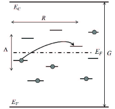
Figure 18: Electron hopping between the localized states in the proximity of Fermi level.

The approach is based on estimating the electron hopping diffusion coefficient

$$D\sim\nu R^{2}$$

where $\nu$ is the hopping frequency. The electron mobility can be then expressed through the Einstein relation

$$\mu=\frac{D}{k_{B}T}$$

so that the conductivity $\sigma=ne\mu$, with the effective electron concentration $n$ corresponding to the states in the energy band $\Delta$, i. e. $n\sim g\Delta$ where $g$ (cm^-3eV^-1) is the electron density of states. We assume $g$ to be energy independent.

The probability of inter-center transition is a product of probabilities of tunneling ($\exp(-2r/a)$) and thermal activation ($\exp(-\Delta/k_{B}T)$) where $a$ is the radius of the electron wave function on a defect. The latter implies that the electron trajectory composed of sequential inter-center transitions can be represented by a set of resistors in series with the hardest link corresponding to the activation by the entire bandwidth $\Delta$. As a result the probability of hopping becomes

$$\nu=\nu_{0}exp\left(-\frac{\Delta}{k_{B}T}-\frac{2r}{a}\right)$$ (46)

where $\nu_{0}$ is the frequency of (hopping) attempt, of the order of the characteristic phonon frequency 10¹³ s^-1.

Given the probability in Eq. (46), it is obviously desirable to make both $\Delta$ and $R$ as small as possible. However, it is rather unlikely that both of these quantities are simultaneously small. To the contrary, it is quite intuitive that the closest center (minimum $R$) will typically have a significant energy difference with that of the original electron location, and vice versa, to find a center that is very close in energy, one will have to look far enough from its original location, hence, large $R$.

The typical situation corresponds to the condition that the center of destination is found with certainty in a volume of $R^{3}$ within the energy band $\Delta$, that is

$$gR^{3}\Delta\sim 1.$$

The latter condition presents the competition between $\Delta$ and $R$ explicitly: the smaller the one the bigger the other.

Expressing $\Delta\sim 1/R^{3}g$ and substituting this into Eq. (46) gives the exponent in which one term increases with $R$ while the other decreases. This competition resolves in the optimum values given (to within numerical factors) by

$$\Delta=k_{B}T\left(\frac{T_{0}}{T}\right)^{1/4},\quad R=a\left(\frac{T_{0}}{T}\right)^{1/4},\quad T_{0}\equiv\frac{1}{ga^{3}k_{B}}.$$ (47)

We note that the effective temperature $T_{0}$ is very much higher than $T$. Indeed, assuming the typical order-of -magnitude estimate $g\sim 10^{19}$ cm^-3eV^-1 and $a\sim 10\AA$ yields $T_{0}\sim 10^{6}$ K. Hence, $(T_{0}/T)^{1/4}\sim 10$ when $T\sim 100K$: the electron hops across the distances and energies by order of magnitude greater than its wave function length and temperature respectively.

Substituting the optimum values from Eq. (47) into Eq. (46) leads to the famous Mott law mott for the variable range hopping conduction,

$$\sigma=\sigma_{0}\exp\left[-\left(\frac{T_{0}}{T}\right)^{1/4}\right],\quad\sigma_{0}\sim ge^{2}\nu_{0}k_{B}T\left(\frac{T_{0}}{T}\right)^{1/4}$$

verified experimentally for many different amorphous semiconductors.

IV.3.2 Band Tails

In disordered systems, such as doped semiconductors (impurity atoms occupying random positions) or amorphous silicon, or window and other glasses, the concept of forbidden gap undergoes certain changes compared to a perfectly ordered ideal crystal. This happens for obvious reasons: the system ceases to be invariant with respect to translations, imperfections are everywhere in the form of valence angle fluctuations, dangling bonds, fluctuations in chemical composition, etc. mieghem In particular, well defined edges of conduction and valence bands become fuzzy, and instead of sharp boundaries give rise to rather diffuse tails of states gradually decaying into what is now called the mobility gap (Fig. 19).

Figure 19: Tails of density of states (DOS) of conduction and valence bands (shown in dash) decay into mobility edge with the characteristic energy scales $\varepsilon$.

A number of different theories, from different perspectives, are in existence. We describe one such more intuitive theory, according to which band tails originate from local fluctuations in atomic potentials felt by the electron or hole. These potentials are thought of as short-range potential wells (say, associated with impurity atoms), whose concentration $n$ undergoes statistical fluctuations with the characteristic dispersion $\sqrt{N}$, where $N$ is the total number of atoms in a volume $R^{3}$ (Fig. 20).

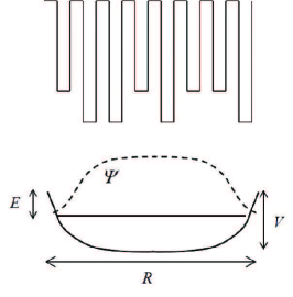
Figure 20: Top: Fluctuation in impurity atom concentration. Bottom: Impurity atoms have stronger short-range potential wells that altogether act as the effective potential well of depth $V$ and length $R$ capable of localizing the electron, whose wave function is shown by dashed line.

To describe DOS in the band tail we proceed from the probability of Gaussian fluctuations

$$p\sim\exp\left[-\frac{(\delta N)^{2}}{\overline{N}}\right]=\exp\left[-\frac{\delta nR^{3}}{\overline{n}}\right]$$ (48)

for the fluctuation of $\delta N$ particles against the background of their average number $\overline{N}$ in the volume $R^{3}$. The greater the fluctuation $\delta n$ in defect concentration, the deeper the effective potential well for the electron and correspondingly the deeper the energy level in the tail.

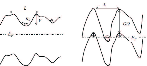
Figure 21: Left: Long range random potential fluctuations in the case of significant screening charge carrier concentration $n_{S}\gg n_{G}$ (but still $n_{S}\ll N$). Right: Same in the case of very low screening concentration $n_{S}\ll n_{G}$.

The latter probability exponentially increases when $\delta n$ or $R$ decrease. However, they cannot be made arbitrarily small because the corresponding potential well then become too shallow (small $\delta n$) and too narrow (small $R$) to accommodate a state of given energy

$$E\sim\frac{\hbar^{2}}{m^{*}R^{2}}-\gamma\delta n.$$ (49)

Here, the first and second terms represent the kinetic and potential electron energy respectively, and $\gamma$ is the proportionality coefficient between the potential well depth $V$ and the concentration fluctuation $n$: $V=\gamma\delta n$.

Expressing $\delta n$ from Eq. (49) and substituting into Eq. (48) gives

$$p\sim\exp\left[-\frac{(E-\hbar^{2}/mR^{2})^{2}R^{3}}{\overline{n}}\right].$$

Optimizing the latter with respect to $R$ gives $R\sim\hbar/\sqrt{m^{*}E}$ and the exponentially decaying DOS,

$$g(E)\propto\exp\left(-\sqrt{\frac{E}{E_{0}}}\right),\quad E_{0}\equiv\frac{m^{*3}\gamma^{4}\overline{n}^{2}}{\hbar^{6}}.$$ (50)

Note that while the above outlined efficient optimization of the exponent can result in a rather approximate result missing a significant numerical multiplier, mieghem which is practically important when the exponent is large. Also, the presence of such a multipler is rather unusual against the background of the majority of approximate methods where such multipliers are typically of the order of unity.

IV.3.3 Random Potential

Here, we briefly discuss variations in potential energy due to randomly distributed charged centers in semiconductors. shklovskii1984 We assume that such centers are randomly distributed in doped and compensated semiconductors. In a volume of linear dimension $L$, their average number is $\overline{N}=\overline{n}L^{3}$ where $n$ is their concentration, and the characteristic fluctuations are given by: $\delta N=\sqrt{N}$.

The corresponding charge fluctuation is a sum of positive and negative centers’ contributions. They are close to each other when the degree of compensation is high enough, $\delta Q=q(\delta N_{+}+\delta N_{-})\approx 2q\sqrt{N}$. The corresponding electric potential fluctuations become,

$$\delta\phi\sim\frac{\delta Q}{\epsilon L}\sim\frac{\sqrt{\overline{n}L}}{\epsilon}$$ (51)

where $\epsilon$ is the dielectric permittivity. We observe that $\delta\phi$ diverges with $L$.

The above potential fluctuations (Fig. 21) do not become infinitely large due to charge carrier screening that we now discuss. Lets assume first that the compensation is not exact and there exists a small concentration $n_{S}=|N_{+}-N_{-}|\ll N_{+}$ of mobile charge carriers. The screening is achieved when the average charge concentration fluctuation $\delta N/L^{3}$ becomes comparable with $n_{S}$, i. e.

$$L\sim\overline{n}^{-1/3}\left(\frac{\overline{n}}{n_{S}}\right)^{2/3}.$$ (52)

If the ratio $\overline{n}/n_{S}$ is not too large (compensation not too strong) then $L\sim\overline{n}^{-1/3}$ is of the order of the average inter-center distance, and the corresponding $\phi$ is not particularly significant. However, in the case of really strong compensation and large ratio $\overline{n}/n_{S}\gg 1$, the screening length gets much longer, and -using Eq. (52)- the potential fluctuation becomes

$$\delta\phi\sim\frac{q\overline{n}^{2/3}}{\epsilon n_{S}^{1/3}}.$$ (53)

The latter estimate holds until the fluctuation amplitude becomes comparable to $G/2$ where $G$ is the forbidden gap, i. e.

$$n_{S}\gg n_{G}=\overline{n}\left(\frac{q\overline{n}^{1/3}}{\epsilon G}\right)^{3}.$$

In the opposite limiting case of $n_{S}\ll n_{G}$, (where $n_{G}$ is the electron concentration within the forbidden gap $G$) the electric potential fluctuations of the conduction and valence bands overlap forming metal type areas where the band edges cross the Fermi level (Fig. 21).

In reality, it is rather hard, if possible at all, to achieve a significant degree of compensation leading to strong enough potential fluctuations in Eq. (53). However, some materials, such as A2B6 semiconductors, are known for their ability of ‘self-compensation’. Practically, this means that they strongly resist doping: introducing donors in these materials trigger the energetically favorable defect creation. The newly created defects of acceptor type compensate the original donors: the electrons leave positively charged donor centers and localize at acceptor defects making them negatively charged . The degree of self-compensation is so high that introducing up to $N\sim 10^{19}$ cm^-3 of doping impurities results in as low as 10¹⁴ cm^-3 charge carrier concentration identifiable with $n_{S}$; hence, $n_{S}\ll N$.

V Conclusions

We hope that the above material reflects to a certain extent the diversity of models, methods and techniques in condensed matter physics and shows how the inductive approach becomes particularly fruitful for such a subject. We fully expect to hear that the reader will find our selection biased and emphasizing some topics at the expense of others. We hope that other instructors and researchers will make broadly available their qualitative methods related to a variety of other subjects and that this effort will provide an example of how that can be achieved.

The above set of examples appears accessible to college and grad students and can be blended indeed into the existing condensed matter curricula. We have successfully used those examples teaching upper undergrad and graduate level courses, such as Solid State Physics, Condensed Matter Physics, and Qualitative Methods in Physics. We have observed higher student enthusiasm toward both in-class and home assignments compared to the standard curriculum items. We attribute that positive feedback to an appreciation for the shorter learning curve provided by the qualitative methods along with their inductive approach being natural to our cognition. The injection of qualitative methods will arm not only students, but acting professionals as well, with the toolkit needed as they deal with the demands of technology -driven environments.

Appendices

Appendix A Perturbation theory for adjacent levels

Figure 22: Perturbation for adjacent levels.

We start with $E_{1}(r)$ and $E_{2}(r)$, the energies of two states vs some parameter $r$, the physical meaning of which can vary between different problems. For example, $E_{1}(r)$ and $E_{2}(r)$ can stand for the energy levels of 2p and 1s states in a well formed by a Coulomb attractive potential with a short range hump of height $U_{0}$ at its center as a function of $U_{0}$, in which case these states can have the same energies at a certain $U_{0}$. Alternatively, $E_{1}(r)$ and $E_{2}(r)$ can stand for the energies of two electron terms in a diatomic molecule vs. its interatomic distance as implied in Fig. 9; they can equally describe the energy levels in a double well potential given in Eq. (10). Similarly, they can represent the electron energies $E_{1}(k)$ and $E_{2}(k)$ vs. their wave vectors $k_{1}$, $k_{2}$ as implied in Sec. IV.1.2.

In all such cases where two energy levels are very close to each other, one can neglect the effects of all other energy levels in a system dealing with a two-state basis, which makes the system solvable exactly. Because of its simplicity, the description in this Appendix turns out to be extremely useful with a variety of applications; yet it remains presented insufficiently in standard curricula.

Following Landau and Lifshitz, landauqm we consider a point $r_{0}$ where $E_{1}(r)$ and $E_{2}(r)$ are close but not equal, such that a change $\delta r\ll r$ makes $E_{1}$ and $E_{2}$ equal. That common value of energy $E$, is the eigenvalue of the Schrödinger equation

$$(\hat{H_{0}}+\hat{V})\Psi=E\Psi.$$ (54)

where $\hat{H_{0}}$ is the unperturbed Hamiltonian and $\hat{V}$ is a small perturbation caused by $\delta r$. The unperturbed wave functions satisfy

$$\hat{H_{0}}\Psi_{1,2}=E_{1,2}\Psi_{1,2}.$$

As a first-order approximation, we consider the superposition $\Psi=C_{1}\Psi_{1}+C_{2}\Psi_{2}.$ Substituting $\Psi$ into Eq. (54 ) leads to

$$c_{1}(E_{1}+\hat{V}-E)\psi_{1}+c_{2}(E_{2}+\hat{V}-E)\psi_{2}=0.$$

Multiplying this equation by $\psi^{*}{{}_{1}}$ or $\psi^{*}{{}_{1}}$, and integrating (taking into account that $\psi_{1}$ and $\psi_{2}$ are orthogonal) one gets,

$$c_{1}(E_{1}+V_{11}-E)+c_{2}V_{12}=0$$ (55)

$$c_{1}V_{21}+c_{2}(E_{2}+V_{22}-E)=0$$ (56)

where $V_{ij}=\int\psi^{*}{{}_{i}}\hat{V}\psi_{j}d^{3}r$. Since $\hat{V}$ is hermitian, $V_{11}$ and $V_{22}$ are real, and $V_{12}=V^{*}_{21}$. For the system of the above two equations to have a non-trivial solution, we need the discriminant to be equal to zero, which yields a quadratic equation for $E$ with two solutions,

$$E=E_{\pm}\equiv\frac{1}{2}(E_{1}+E_{2}+V_{11}+V_{22})$$

$$\pm\sqrt{\frac{1}{4}(E_{1}-E_{2}+V_{11}-V_{22})^{2}+|V_{12}|^{2}}$$ (57)

By denoting $E_{1}+V_{11}=E_{1}^{(0)}$, $E_{2}+V_{22}=E_{2}^{(0)}$ and $V_{12}V^{*}_{21}=V_{0}^{2}$ finally yields,

$$E_{\pm}=\frac{E_{1}^{(0)}+E_{2}^{(0)}}{2}\pm\sqrt{\frac{(E_{1}^{(0)}-E_{2}^{(0)})^{2}}{4}+V_{0}^{2}}.$$ (58)

The latter result is illustrated in Fig. 22. To the accuracy of notations, it reduces to that in Eqs. (10) and (29).

References

- (1) V. G. Karpov, and Maria Patmiou, Physics in the information age: qualitative methods (with examples from quantum mechanics), https://arxiv.org/pdf/1907.08154.pdf.
- (2) National Research Council, How People Learn: Brain, Mind, Experience, and School: Expanded Edition. (The National Academies Press, Washington, DC, 2000),172-188.
- (3) N.C. Yeh, A Perspective of Frontiers in Modern Condensed Matter Physics, AAPPS Bulletin, 18 2,11-29 (2008).
- (4) N. Ashcroft and N. Mermin, Solid State Physics, (Hartcourt College Publishing, 1976).
- (5) Y. M. Galperin, V. G. Karpov, V. I. Kozub, Localized states in glasses, Adv. Phys.,38, 669 (1989).
- (6) C. Kittel, Introduction to Solid State Physics, Wiley, New York, London (1953).
- (7) A. B. Migdal, Qualitative Methods in Quantum Theory (Perseus Publishing, Cambridge,1977).
- (8) L. D. Landau, E. M. Lifshitz Theory of elesticity 3rd edition, (Butterworth Heinemann, 1986).
- (9) B. B. Mandelbrot, The Fractal Geometry of Nature, (W.H. Freeman and Company, 1997).
- (10) S. Alexander and R. Orbach, Density of states on fractals: ”fractons”. Journal de Physique Lettres, Edp sciences, 43 (17), 625-631 (1982).
- (11) T. B. Schrder and J. C. Dyre, Ac hopping conduction at extreme disorder takes place on the percolating cluster, preprint available at arXiv:0801.0531v4[cond-mat.dis-nn]6Jun2008
- (12) S. Sze and K. Ng, Physics of Semiconductor Devices 3rd edition, (Wiley, 2007).
- (13) C. Kittel Introduction to Solid State Physics 7th edition, (Wiley, 1996).
- (14) L. D. Landau, E. M. Lifshitz Quantum Mechanics, 2nd edition (Pergamon Press, Bristol, 1965).
- (15) L. D. Landau ”Über die Bewegung der Elektronen in Kristallgitter”. Phys. Z. Sowjetunion. 3, 644 (1933). L. D. Landau, S.I. Pekar, Effective mass of a polaron, Zh. Eksp. Teor. Fiz. 18, 419–423 (1948) [in Russian], available at: https://web.archive.org/web/20160305170544/http://ujp.bitp.kiev.ua/files/journals/53/si/53SI15p.pdf
- (16) P. W. Anderson, Model for the Electronic Structure of Amorphous Semiconductors, Phys. Rev. Lett. 34, 953-955 (1975)
- (17) J. Hubbard, Electron Correlations in Narrow Energy Bands, Proceedings of the Royal Society of London. 276, (1365) 238–257 (1963)
- (18) N. F. Mott and E. A. Davis, Electronic Processes in Non-crystalline Materials Clarendon, Oxford, 1979.
- (19) S. D. Baranovskii, V. G. Karpov, Multiphonon hopping conduction, Fiz. Tekh. Poluprovodn. 20, 1811(1986) [Sov. Phys. Semicond. 20, 1137 (1986)]
- (20) A. Chatterjee, S. Mukhopadhyay, Polarons and Bipolarons: An Introduction, CRS Press (2018).
- (21) P. Mieghem, Theory of band tails in heavily doped semiconductors, Rev. Mod. Phys.64, (3) 755-793 (1992)
- (22) B. I. Shklovskii, A.L.Efros, Electronic properties of doped semiconductors, Springer, Heidelberg,1984.