Learning Multi-Object Tracking and Segmentation from Automatic Annotations

Abstract

In this work we contribute a novel pipeline to automatically generate training data, and to improve over state-of-the-art multi-object tracking and segmentation (MOTS) methods. Our proposed track mining algorithm turns raw street-level videos into high-fidelity MOTS training data, is scalable and overcomes the need of expensive and time-consuming manual annotation approaches. We leverage state-of-the-art instance segmentation results in combination with optical flow predictions, also trained on automatically harvested training data. Our second major contribution is MOTSNet– a deep learning, tracking-by-detection architecture for MOTS – deploying a novel mask-pooling layer for improved object association over time. Training MOTSNet with our automatically extracted data leads to significantly improved sMOTSA scores on the novel KITTI MOTS dataset (+1.9%/+7.5% on cars/pedestrians), and MOTSNet improves by +4.1% over previously best methods on the MOTSChallenge dataset. Our most impressive finding is that we can improve over previous best-performing works, even in complete absence of manually annotated MOTS training data.

1 Introduction and Motivation

We focus on the challenging task of multi-object tracking and segmentation (MOTS) [47], which was recently introduced as an extension of bounding-box based multi-object tracking. Joining instance segmentation with tracking was shown to noticeably improve tracking performance, as unlike bounding boxes, instance segmentation masks do not suffer from overlapping issues but provide fine-grained, pixel-level information about objects to be tracked.

While this finding is encouraging, it comes with the downside of requiring pixel-level (typically polygon-based) annotations, which are known to be time-consuming in generation and thus expensive to obtain. The works in [9, 33] report annotation times of $\approx$90 minutes per image, to manually produce high-quality panoptic segmentation masks. Analogously, it is highly demanding to produce datasets for the MOTS task where instance segmentation masks need to also contain tracking information across frames.

To avoid generating MOTS labels completely from scratch and in a purely manual way, [47] has followed the semi-automatic annotation procedure from [4], and extended the existing multi-object tracking datasets KITTI tracking [11] (i.e. 21 sequences from the raw KITTI dataset) and MOTChallenge [32] (4/7 sequences). These datasets already provide bounding box-based tracks for cars and pedestrians. Instance segmentation masks were generated as follows. First, two segmentation masks per object were generated by human annotators (which also had to chose the objects based on diversity in the first place). Then, DeepLabV3+ [6], i.e. a state-of-the-art semantic segmentation network, was trained on the initially generated masks in a way to overfit these objects in a sequence-specific way, thus yielding reasonable segmentation masks for the remaining objects in each track. The resulting segmentation masks then underwent another manual correction step to fix remaining errors. Finally, these automatic and manual steps were iterated until convergence.

Including an automated segmentation algorithm is clearly speeding up the MOTS dataset generation process, but still has significant shortcomings. Most importantly, the approach in [47] still depends on the availability of bounding-box based, multi-object tracking information as provided by datasets like [11, 32]. Also, their remaining human annotation effort for generating initial instance masks was considerable, i.e. [47] reports that $\approx$8k masks (or $12.3\%$ of all masks in KITTI MOTS) had been manually labeled before fine-tuning a (modified) DeepLabV3+ segmentation network, pre-trained on COCO [24] and Mapillary Vistas [33]. Finally, such an approach cannot be expected to generalize well for generating orders of magnitude more training data.

In this paper we introduce a novel approach for automatically generating high-quality training data (see Fig. 1 for an example) from generic street-level videos for the task of joint multi-object tracking and segmentation. Our methods are conceptually simple and leverage state-of-the-art instance [12] (or Panoptic [39, 8]) segmentation models trained on existing image datasets like Mapillary Vistas [33] for the task of object instance segmentation. We further describe how to automatically mine tracking labels for all detected object instances, building upon state-of-the-art optical flow models [53], that in turn have been trained on automatically harvested flow supervision obtained from image-based 3d modeling (structure-from-motion).

Another important contribution of our paper is MOTSNet, a deep learning, tracking-by-detection approach for MOTS. MOTSNet takes advantage of a novel mask-pooling layer, which allows it to exploit instance segmentation masks to compute a representative embedding vector for each detected object. The tracking process can then be formulated as a series of Linear Assignment Problems (LAP), optimizing a payoff function which compares detections in the learned embedding space.

We demonstrate the superior quality for each step of our proposed MOTS training data extraction pipeline, as well as the efficacy of our novel mask-pooling layer. The key contributions and findings of our approach are:

• Automated MOTS training data generation – instance detection, segmentation and actual tracking – is possible at scale and with very high fidelity, approximating the quality of previous state-of-the-art results [47] without even directly training for it.

• Deep-learning based, supervised optical flow [53] can be effectively trained on pixel-based correspondences obtained from Structure-from-Motion and furthermore used for tracklet extraction.

• Direct exploitation of instance segmentation masks through our proposed mask-pooling layer yields to significant improvements of sMOTSA scores

• The combination of our general-purpose MOTS data generation pipeline with our proposed MOTSNet improves by up to 1.2% for cars and 7.5% for pedestrians over the previously best method on KITTI MOTS in absolute terms, while using $13.7\%$ fewer parameters.

We provide extensive ablation studies on the KITTI MOTS, MOTSChallenge, and Berkeley Deep Drive BDD100k [54] datasets and obtain results consistently improving with a large margin over the prior state-of-the-art [47].

2 Related Works

Since the MOTS task was only very recently introduced in [47], directly related works are scarce. Instead, the bulk of related works in a broader sense comes from the MOT (multi-object tracking) and VOS (video object segmentation) literature. This is true in terms of both, datasets (see e.g. [11, 21, 32] for MOT and [37, 40, 23] for VOS/VOT, respectively), and methods tackling the problems ([44] for MOT and [52, 29, 35, 48] for VOS).

Combining motion and semantics.

The work in [17] uses semantic segmentation results from [27] for video frames together with optical flow predictions from EpicFlow [41] to serve as ground truth, for training a joint model on future scene parsing, i.e. the task of anticipating future motion of scene semantics. In [28] this task is extended to deal with future instance segmentation prediction, based on convolutional features from a Mask R-CNN [12] instance segmentation branch. In [16] a method for jointly estimating optical flow and temporally consistent semantic segmentation from monocular video is introduced. Their approach is based on a piece-wise flow model, enriched with semantic information through label consistency of superpixels.

Semi-automated dataset generation.

Current MOT [49, 32, 11] and VOS [51, 38] benchmarks are annotated based on human efforts. Some of them, however, use some kind of automation. In [51], they exploit the temporal correlation between consecutive frames in a skip-frame strategy, although the segmentation masks are manually annotated. A semi-automatic approach is proposed in [1] for annotating multi-modal benchmarks. It uses a pre-trained VOS model [18] but still requires additional manual annotations and supervision on the target dataset. The MOTS training data from [47] is generated by augmenting an existing MOT dataset [32, 11] with segmentation masks, using the iterative, human-in-the-loop procedure we briefly described in Sec. 1. The tracking labels on [32, 11] were manually annotated and, in the case of [32], refined by adding high-confidence detections from a pedestrian detector.

The procedures used in these semi-automatic annotation approaches often resemble those of VOS systems which require user input to select objects of interest in a video. Some proposed techniques in this field [7, 5, 31] are extensible to multiple object scenarios. A pixel-level embedding is built in [7] to solve segmentation and achieve state-of-the-art accuracy with low annotation and computational cost.

To the best of our knowledge, the only work that generates tracking data from unlabeled large-scale videos is found in [36]. By using an adaptation of the approach in [35], Osep et al. perform object discovery on unlabeled videos from the KITTI Raw [10] and Oxford RobotCar [30] datasets. Their approach however cannot provide joint annotations for instance segmentation and tracking.

Deep Learning methods for MOT and MOTS.

Many deep learning methods for MOTS/VOS are based on “tracking by detection”, i.e. candidate objects are first detected in each frame, and then joined into tracks as a post-processing step (e.g. [47]). A similar architecture, i.e. a Mask R-CNN augmented with a tracking head, is used in [52] to tackle Video Instance Segmentation. A later work [29] improved over [52] by adapting the UnOVOST [55] model that, first in an unsupervised setting, uses optical flow to build short tracklets later merged by a learned embedding. For the plain MOT task, Sharma et al. [44] incorporated shape and geometry priors into the tracking process.

Other works instead, perform detection-free tracking. CAMOT [35] tracks category-agnostic mask proposals across frames, exploiting both appearance and geometry cues from scene flow and visual odometry. Finally, the VOS work in [48], follows a correlation-based approach, extending popular tracking models [3, 22]. Their SiamMask model only requires bounding box initialization but is pre-trained on multiple, human-annotated datasets [24, 51, 43].

3 Dataset Generation Pipeline

Our proposed data generation approach is rather generic w.r.t. its data source, and here we focus on the KITTI Raw [10] dataset. KITTI Raw contains 142 sequences (we excluded the 9 sequences overlapping with the validation set of KITTI MOTS), for a total of $\sim 44$k images, captured with a professional rig including stereo cameras, LiDAR, GPS and IMU. Next we describe our pipeline which, relying only on monocular images and GPS data is able to generate accurate MOTS annotations for the dataset.

3.1 Generation of Instance Segmentation Results

We begin with segmenting object instances in each frame per video and consider a predefined set $\mathcal{Y}$ of $37$ object classes that belong to the Mapillary Vistas dataset [33]. To extract the instance segments, we run the Seamless Scene Segmentation method [39], augmented with a ResNeXt-101-32$\times$8d [50] backbone and trained on Mapillary Vistas. By doing so, we obtain a set of object segments $\mathcal{S}$ per video sequence. For each segment $s\in\mathcal{S}$, we denote by $t_{s}\geq 0$ the frame where the segment was extracted, by $y_{s}\in\mathcal{Y}$ the class it belongs to and by $\phi_{s}:\mathbb{R}^{2}\to\{0,1\}$ a pixel indicator function representing the segmentation mask, i.e. $\phi_{s}(i,j)=1$ if and only if pixel $(i,j)$ belongs to the segment. For convenience, we also introduce the notation $\mathcal{S}_{t}$ to denote the set of all segments extracted from frame $t$ of a given video. For KITTI Raw we roughly extracted 1.25M segments.

3.2 Generation of Tracklets using Optical Flow

After having automatically extracted the instance segments from a given video in the dataset, our goal is to leverage on optical flow to extract tracklets, i.e. consecutive sequences of frames where a given object instance appears.

Flow training data generation.

We automatically generate ground-truth data for training an optical flow network by running a Structure-from-Motion (SfM) pipeline, namely OpenSfM, on the KITTI Raw video sequences and densify the result using PatchMatch [45]. To further improve the quality of the 3d reconstruction, we exploit the semantic information that has been already extracted per frame to remove spurious correspondences generated by moving objects. Consistency checks are also performed in order to retain correspondences that are supported by at least $3$ images. Finally, we derive optical flow vectors between pairs of consecutive video frames in terms of the relative position of correspondences in both frames. This process produces sparse optical flow, which will be densified in the next step.

Flow network.

We train a modified version of the HD³ flow network [53] on the dataset that we generated from KITTI Raw, without any form of pre-training. The main differences with respect to the original implementation are the use of In-Place Activated Batch Norm (iABN) [42], which provides memory savings that enable the second difference, namely the joint training of forward and backward flow. We then run our trained flow network on pairs of consecutive frames in KITTI Raw in order to determine a dense pixel-to-pixel mapping between them. In more detail, for each frame $t$ we compute the backward mapping $\overleftarrow{f}_{t}:\mathbb{R}^{2}\to\mathbb{R}^{2}$, which provides for each pixel of frame $t$ the corresponding pixel in frame $t-1$.

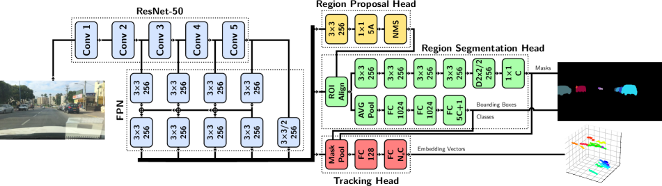
Figure 2: Overview of the MOTSNet architecture. Blue: network backbone; yellow: Region Proposal Head; green: Region Segmentation Head; red: Tracking Head. For an in-depth description of the various components refer to Sec. 4.1 in the text.

Tracklet generation.

In order to represent the tracklets that we have collected up to frame $t$, we use a graph $\mathcal{G}_{t}=(\mathcal{V}_{t},\mathcal{T}_{t})$, where vertices are all segments that have been extracted until the $t$th frame, i.e. $\mathcal{V}_{t}=\bigcup_{j\geq 1}^{t}\mathcal{S}_{j}$, and edges $\mathcal{T}_{t}\subseteq\mathcal{V}_{t}^{2}$ provide the matching segments across consecutive frames. We start by initializing the graph in the first frame as $\mathcal{G}_{1}=(\mathcal{S}_{1},\emptyset)$. We construct $\mathcal{G}_{t}$ for $t>1$ inductively from $\mathcal{G}_{t-1}$ using the segments $\mathcal{S}_{t}$ extracted at time $t$ and the mapping $\overleftarrow{f}_{t}$ according to the following procedure. The vertex set $\mathcal{V}_{t}$ of graph $\mathcal{G}_{t}$ is given by the union of the vertex set $\mathcal{V}_{t-1}$ of $\mathcal{G}_{t-1}$ and $\mathcal{S}_{t}$, i.e. $\mathcal{V}_{t}=\mathcal{V}_{t-1}\cup\mathcal{S}_{t}$. The edge set is computed by solving a linear assignment problem between $\mathcal{S}_{t-1}$ and $\mathcal{S}_{t}$, where the payoff function is constructed by comparing segments in $\mathcal{S}_{t}$ against segments in $\mathcal{S}_{t-1}$ warped to frame $t$ via the mapping $\overleftarrow{f}_{t}$. We design the payoff function $\pi(\hat{s},s)$ between a segment $\hat{s}\in\mathcal{S}_{t-1}$ in frame $t-1$ and a segment $s\in\mathcal{S}_{t}$ in frame $t$ as follows:

$$\pi(\hat{s},s)=\text{IoU}(\phi_{s},\phi_{\hat{s}}\circ\overleftarrow{f}_{t})+\eta(\hat{s},s)\,,$$

where $\text{IoU}(\cdot,\cdot)$ computes the Intersection-over-Union of the two masks given as input, and $\eta(\hat{s},s)\in\{-\infty,0\}$ is a characteristic function imposing constraints regarding valid mappings. Specifically, $\eta(\hat{s},s)$ returns $0$ if and only if the two segments belong to the same category, i.e. $y_{\hat{s}}=y_{s}$, and none of the following conditions on $s$ hold:

• $b_{1}(s)-b_{2}(s)<\tau_{0}$

• $b_{1}(s)<\tau_{1}$, and

• $b_{1}(s)/r(s)<\tau_{2}$,

where $b_{1}(s)$ and $b_{2}(s)$ denote the largest and second-largest areas of intersection with $s$ obtained by segments warped from frame $t-1$ and having class $y_{s}$, and $r(s)$ denotes the area of $s$ that is not covered by segments of class $y_{s}$ warped from frame $t-1$. We solve the linear assignment problem using the Hungarian algorithm, by maximizing the total payoff under a relaxed assignment constraint, which allows segments to remain unassigned. In other terms, we solve the following optimization problem:

maximize $$\sum_{s\in\mathcal{S}_{t}}\sum_{\hat{s}\in\mathcal{S}_{t-1}}\pi(\hat{s},s)\alpha(\hat{s},s)\,$$ (1)

s.t. $$\mathop{\eqmakebox[A]{$\displaystyle\sum_{s\in\mathcal{S}_{t}}$}}\alpha(\hat{s},s)\leq 1\qquad\forall\hat{s}\in\mathcal{S}_{t-1}$$ (2)

$$\mathop{\eqmakebox[A]{$\displaystyle\sum_{\hat{s}\in\mathcal{S}_{t-1}}$}}\alpha(\hat{s},s)\leq 1\qquad\forall s\in\mathcal{S}_{t}$$ (3)

$$\alpha(\hat{s},s)\in\{0,1\}\quad\forall(\hat{s},s)\in\mathcal{S}_{t-1}\times\mathcal{S}_{t}\,.$$ (4)

Finally, the solution $\alpha$ of the assignment problem can be used to update the set of edges $\mathcal{T}_{t}$, i.e. $\mathcal{T}_{t}=\mathcal{T}_{t-1}\cup\alpha^{-1}(1)$, where $\alpha^{-1}(1)$ is the set of matching segments, i.e. the pre-image of $1$ under $\alpha$.

Note that this algorithm cannot track objects across full occlusions, since optical flow is unable to infer the trajectories of invisible objects. When training MOTSNet however, we easily overcome this limitation with a simple heuristic, described in Sec. 4.2, without needing to join the tracklets into full tracks.

4 MOTSNet

Here we describe our multi-object tracking and segmentation approach. Its main component is MOTSNet (see Sec. 4.1), a deep net based on the Mask R-CNN [12] framework. Given an RGB image, MOTSNet outputs a set of instance segments, each augmented with a learned embedding vector which represents the object’s identity in the sequence (see Sec. 4.2). The object tracks are then reconstructed by applying a LAP-based algorithm, described in Sec. 4.3.

4.1 Architecture

MOTSNet’s architecture follows closely the implementation of Mask R-CNN described in [39], but addtionally comprises a Tracking Head (TH) that runs in parallel to the Region Segmentation Head (RSH) (see Figure 2). The “backbone” of the network is composed of an FPN [25] component on top of a ResNet-50 body [13], producing multi-scale features at five different resolutions. These features are fed to a Region Proposal Head (RPH), which predicts candidate bounding boxes where object instances could be located in the image. Instance specific features are then extracted from the FPN levels using ROI Align [12] in the areas defined by the candidate boxes, and fed to the RSH and the TH. Finally, for each region, the RSH predicts a vector of class probabilities, a refined bounding box and an instance segmentation mask. Synchronized InPlace-ABN [42] is employed throughout the network after each layer with learnable parameters, except for those producing output predictions. For an in-depth description of these components we refer the reader to [39].

Tracking Head (TH).

Instance segments, together with the corresponding ROI Align features from the FPN, are fed to the TH to produce a set of $N_{e}$-dimensional embedding vectors. As a first step, the TH applies “mask-pooling” (described in the section below) to the input spatial features, obtaining 256-dimensional vector features. This operation is followed by a fully connected layer with 128 channels and synchronized InPlace-ABN. Similarly to masks and bounding boxes in the RSH, embedding vectors are predicted in a class-specific manner by a final fully connected layer with $N_{e}\times C$ outputs, where $C$ is the number of classes, followed by L2-normalization to constrain the vectors on the unit hyper-sphere. The output vectors are learned such that instances of the same object in a sequence are mapped close to each other in the embedding space, while instances of other objects are mapped far away. This is achieved by minimizing a batch hard triplet loss, described in Sec. 4.2.

Mask-pooling.

ROI Align features include both foreground and background information, but, in general, only the foreground is actually useful for recognizing an object across frames. In our setting, by doing instance segmentation together with tracking, we have a source of information readily available to discriminate between the object and its background. This can be exploited in a straightforward attention mechanism: pooling under the segmentation mask. Formally, given the pixel indicator function $\phi_{s}(i,j)$ for a segment $s$ (see Sec. 3.1), and the corresponding input $N$-dimensional ROI-pooled feature map $\mathrm{X}_{s}:\mathbb{R}^{2}\to\mathbb{R}^{N}$, mask-pooling computes a feature vector $x_{s}\in\mathbb{R}^{N}$ as:

$$x_{s}=\frac{\sum_{i}\sum_{j}\phi_{s}(i,j)\mathrm{X}_{s}(i,j)}{\sum_{i}\sum_{j}\phi_{s}(i,j)}\,.$$

During training we pool under the ground truth segmentation masks, while at inference time we switch to the masks predicted by the RSH.

4.2 Training Losses

MOTSNet is trained by minimizing the following loss function:

$$L=L_{\text{TH}}+\lambda(L_{\text{RPH}}+L_{\text{RSH}})\,,$$

where $L_{\text{RPH}}$ and $L_{\text{RSH}}$ represent the Region Proposal Head and Region Segmentation Head losses as defined in [39], and $\lambda$ is a weighting parameter.

$L_{\text{TH}}$ is the loss component associated with the Tracking Head, i.e. the following batch hard triplet loss [15]:

$$L_{\text{TH}}=\frac{1}{|\mathcal{S}_{B}|}\sum_{s\in\mathcal{S}_{B}}\max(\max_{\hat{s}\in\mu_{B}(s)}\|a_{s}^{y_{s}}-a_{\hat{s}}^{y_{\hat{s}}}\|\\ -\min_{\hat{s}\in\bar{\mu}_{B}(s)}\|a_{s}^{y_{s}}-a_{\hat{s}}^{y_{\hat{s}}}\|+\beta,0)\,,$$

where $\mathcal{S}_{B}$ is the set of predicted, positive segments in the current batch, $a_{s}^{y_{s}}$ is the class-specific embedding vector predicted by the TH for a certain segment $s$ and ground truth class $y_{s}$, and $\beta$ is a margin parameter. The definition of a “positive” segment follows the same logic as in the RSH (see [39]), i.e. a segment is positive if its bounding box has high IoU with a ground truth segment’s bounding box. The functions $\mu_{B}(s)$ and $\bar{\mu}_{B}(s)$ map $s$ to the sets of its “matching” and “non-matching” segments in $\mathcal{S}_{B}$, respectively. These are defined as:

$$\mu_{B}(s) =\left\{\hat{s}\in\mathcal{S}_{B}\mid y_{s}=y_{\hat{s}}\land M(s,\hat{s})\right\}\,,$$

$$\bar{\mu}_{B}(s) =\left\{\hat{s}\in\mathcal{S}_{B}\mid y_{s}=y_{\hat{s}}\land\neg M(s,\hat{s})\right\}\,,$$

where $M(s,\hat{s})$ is true iff $s$ and $\hat{s}$ belong to the same tracklet in the sequence. Note that we are restricting the loss to only compare embedding vectors of segments belonging to the same class, effectively letting the network learn a set of class-specific embedding spaces.

In order to overcome the issue due to occlusions mentioned in Sec. 3.2, when training on KITTI Synth we also apply the following heuristic. Ground truth segments are only considered in the tracking loss if they are associated with a tracklet that appears in more than half of the frames in the current batch. This ensures that, when an occlusion causes a track to split in multiple tracklets, these are never mistakenly treated by the network as different objects.

4.3 Inference

During inference, we feed frames $t$ through the network, obtaining a set of predicted segments $\mathcal{S}_{t}$, each with its predicted class $y_{s}$ and embedding vector $a_{s}^{y_{s}}$. Our objective is now to match the segments across frames in order to reconstruct a track for each object in the sequence. To do this, we follow the algorithmic framework described in Sec. 3.2, with a couple of modifications. First, we allow matching segments between the current frame and a sliding window of $N_{w}$ frames in the past, in order to be able to “jump” across occlusions. Second, we do not rely on optical flow anymore, instead measuring the similarity between segments in terms of their distance in the embedding space and temporal offset.

More formally, we redefine the payoff function in Eq. (1) as:

$$\pi(\hat{s},s) =-\pi^{*}(\hat{s},s)+\eta(s,\hat{s})\,,$$ (5)

$$\pi^{*}(\hat{s},s) =\|a_{s}^{y_{s}}-a_{\hat{s}}^{y_{\hat{s}}}\|+\frac{|t_{s}-t_{\hat{s}}|}{N_{w}}\,,$$ (6)

where the characteristic function $\eta(s,\hat{s})$ is redefined as:

$$\eta(s,\hat{s})=\begin{cases}0&\text{if}\,y_{s}=y_{\hat{s}}\land\pi^{*}(\hat{s},s)\leq\tau\,,\\ -\infty&\text{otherwise}\,,\end{cases}$$

and $\tau$ is a configurable threshold value. Furthermore, we replace $\mathcal{S}_{t-1}$ in Eq. (2) and Eq. (4) with the set:

$$\mathcal{U}_{t}=\left\{s\in\mathcal{V}_{t-1}\mid t_{s}\geq t-N_{w}\land(s,\hat{s})\notin\mathcal{T}_{t-1}\forall\hat{s}\right\}\,,$$

which contains all terminal (i.e. most recent) segments of the track seen in the past $N_{w}$ frames. As a final step after processing all frames in the sequence, we discard the tracks with fewer than $N_{t}$ segments, as, empirically, very short tracks usually arise from spurious detections.

5 Experiments

We provide a broad experimental evaluation assessing i) the quality of our automatically harvested KITTI Synth dataset on the MOTS task by evaluating it against the KITTI MOTS dataset, ii) demonstrate the effectiveness of MOTSNet and our proposed mask-pooling layer against strong baselines, both on KITTI MOTS and MOTSChallenge, iii) demonstrate the generality of our MOTS label generation process by extending the BDD100k tracking dataset with segmentation masks to become a MOTS variant thereof and iv) provide an ablation about the contribution of association terms for the final track extraction. While we can benchmark the full MOTS performance on KITTI MOTS and MOTSChallenge, we are able to infer the tracking performance based on the ground truth box-based tracking annotations available for BDD100k.

		sMOTSA		MOTSA		MOTSP		mAP
Method	Pre-training	Car	Ped	Car	Ped	Car	Ped	Box	Mask
KITTI Synth (val) + HD3 [53] model zoo	inference only	65.4	45.7	77.3	66.3	87.6	76.6	–	–
KITTI Synth (val) + HD3, KITTI-SfM	inference only	65.5	45.4	77.4	66.0	87.6	76.6	–	–
MOTSNet with:
AveBox+TH	I	73.7	46.4	85.8	62.8	86.7	76.7	57.4	50.9
AveMsk-TH	I	76.4	44.0	88.5	60.3	86.8	76.6	57.8	51.3
AveBox-TH	I	75.4	44.5	87.3	60.8	86.9	76.7	57.5	51.0
KITTI MOTS train sequences only	I	72.6	45.1	84.9	62.9	86.1	75.6	52.5	47.6
MOTSNet	I	77.6	49.1	89.4	65.6	87.1	76.4	58.1	51.8
MOTSNet	I, M	77.8	54.5	89.7	70.9	87.1	78.2	60.8	54.1

Table 1: Results on the KITTI MOTS validation set when training on KITTI Synth. First section: ablation results. Second section: main results and comparison with state of the art. Note that all MOTSNet variants are trained exclusively on machine generated annotations, while TrackR-CNN is trained on human annotated ground truth.

5.1 Evaluation Measures

The CLEAR MOT [2] metrics, including Multi-Object Tracking Accuracy (MOTA) and Precision (MOTP), are well established as a standard set of measures for evaluating Multi-Object Tracking systems. These, however, only account for the bounding box of the tracked objects. Voigtlaender et al. [47] describe an extension of MOTA and MOTP that measure segmentation as well as tracking accuracy, proposing the sMOTSA, MOTSA and MOTSP metrics. In particular, MOTSA and MOTSP are direct equivalents of MOTA and MOTP, respectively, where the prediction-to-ground-truth matching process is formulated in terms of mask IoU instead of bounding box IoU. Finally, sMOTSA can be regarded as a “soft” version of MOTSA where the contribution of each true positive segment is weighted by its mask IoU with the corresponding ground truth segment. Please refer to Appendix A for a formal description of these metrics.

5.2 Experimental Setup

All the results in the following sections are based on the same MOTSNet configuration, with a ResNet-50 backbone and embedding dimensionality fixed to $N_{e}=32$. Batches are formed by sampling a subset of $N_{w}$ full-resolution, contiguous frames at a random offset in one of the training sequences, for each GPU. During training we apply scale augmentation in the $[0.8,1.25]$ range and random flipping. Training by SGD follows the following linear schedule: $\text{lr}_{i}=\text{lr}_{0}(1-\frac{i}{\#\text{steps}})$, where $\text{lr}_{0}$ is the starting learning rate and $i$ is the training step (i.e. batch) index. The network weights are initialized from an ImageNet-pretrained model (“I” in the tables), or from a Panoptic Segmentation model trained on the Mapillary Vistas dataset (“M” in the tables), depending on the experiment. Differently from [47], we do not pre-train on MS COCO [24] (“C” in the tables).

The hyper-parameters of the inference algorithm are set as follows: threshold $\tau=1$; window size $N_{w}$ equal to the per-GPU batch size used during training; minimum track length $N_{t}=5$. Note that, in contrast with [47], we do not fine-tune these parameters, instead keeping them fixed in all experiments, and independent of class. All experiments are run on four V100 GPUs with 32GB of memory.

5.3 KITTI MOTS

The KITTI MOTS dataset was introduced in [47], adding instance segmentation masks for cars and pedestrians to a subset of 21 sequences from KITTI raw [11]. It has a total of 8.008 images (5.027 for training and 2.981 for validation), containing approximately 18.8k/8.1k annotated masks for 431/99 tracks of cars/pedestrians in training, and roughly 8.1k/3.3k masks for 151/68 tracks on the validation split. Approximately $12.3\%$ of all masks were manually annotated and the rest are human-verified and -corrected instance masks. As the size of this dataset is considerably larger and presumably more informative than MOTSChallenge, we focused our ablations on it.

Table 1 summarizes the analyses and experiments we ran on our newly generated KITTI Synth dataset, by evaluating on the official KITTI MOTS validation set. We discuss three types of ablations in what follows.

KITTI Synth data quality analysis.

The two topmost rows of Tab. 1 show the results when generating the validation set results solely with our proposed dataset generation pipeline, described in Section 3, i.e. no learned tracking component is involved. Our synthetically extracted validation data considerably outperforms the sMOTSA scores on pedestrians and almost obtains the performance on cars for CAMOT [35], as reported in [47]. When training the flow network on the training data generated from SfM as described in Section 3, we match the performance obtained by the best-performing HD³ [53] model for KITTI. While this validates our tracklet generation process and the way we harvest optical flow training data, we investigate further the effects of learning from imperfect data (see Sec. 3.2).

MOTSNet tracking head ablations.

The center block in Tab 1 compares different configurations for the Tracking Head described in 4. The first variant (AveBox+TH) replaces the mask-pooling operation in the Tracking Head with average pooling on the whole box. The second and third variants (AveMsk-TH, AveBox-TH) completely remove the Tracking Head and its associated loss, instead directly computing the embeddings by pooling features under the detected mask or box, respectively. All variants perform reasonably well and improve over [35, 34] on the primary sMOTSA metric. Notably, AveMsk-TH, i.e. the variant using our mask-pooling layer and no tracking head, is about on par with TrackR-CNN on cars despite being pre-trained only on ImageNet, using a smaller, ResNet-50 backbone and not exploiting any tracking supervision. The last variant in this block shows the performance obtained when MOTSNet is trained only on images also in the KITTI MOTS training set, and with our full model. Interestingly, the scores only drop to an extent where the gap to [47] might be attributed to their additional pre-training on MS COCO and Mapillary Vistas and a larger backbone (cf. Tab. 2). Finally, comparing the latter directly to our MOTSNet results from Tab. 2 (ImageNet pre-trained only), where we directly trained on KITTI MOTS training data, our KITTI Synth-based results improve substantially on cars, again confirming the quality of our automatically extracted dataset.

The bottommost part of this table shows the performance when training on the full KITTI Synth dataset and evaluating on KITTI MOTS validation, using different pre-training settings. The first is pre-trained on ImageNet and the second on both, ImageNet and Mapillary Vistas. While there is only little gap between them on the car class, the performance on pedestrians rises by over 5% when pre-training on Vistas. The most encouraging finding is that using our solely automatically extracted KITTI Synth dataset we obtain significantly improved scores (+1.6% on cars, +7.4% on pedestrians) in comparison to the previous state-of-the-art method from [47], trained on manually curated data.

MOTSNet on KITTI MOTS.

In Tab. 2 we directly compare against previously top-performing works including TrackR-CNN [47] and references from therein, e.g. CAMOT [35], CIWT [34], and BeyondPixels [44]. It is worth noting that the last three approaches were reported in [47] and partially built on. We provide all relevant MOTS measures together with separate average AP numbers to estimate the quality of bounding box detections or instance segmentation approaches, respectively. For our MOTSNet we again show results under different pre-training settings (ImageNet, Mapillary Vistas and KITTI Synth). Different pre-trainings affect the classes cars and pedestrians in a different way, i.e. the ImageNet and Vistas pre-trained model performs better on pedestrians while the KITTI Synth pre-trained one is doing better on cars. This is most likely due to the imbalanced distribution of samples in KITTI Synth while our variant with pre-training on both, Vistas and KITTI Synth yields the overall best results. We obtain absolute improvements of 1.9%/7.5% for cars/pedestrians over the previously best work in [47] despite using a smaller backbone and no pre-training on MS COCO. Finally, also the recognition metrics for both, detection (box mAP) and instance segmentation (mask mAP) significantly benefit from pre-training on our KITTI Synth dataset, and in conjuction with Vistas rise by 7.2% and 6.4% over the ImageNet pre-trained variant, respectively.

		sMOTSA		MOTSA		MOTSP		mAP
Method	Pre-training	Car	Ped	Car	Ped	Car	Ped	Box	Mask
TrackR-CNN [47]	I, C, M	76.2	47.1	87.8	65.5	87.2	75.7	–	–
CAMOT [35]	I, C, M	67.4	39.5	78.6	57.6	86.5	73.1	–	–
CIWT [34]	I, C, M	68.1	42.9	79.4	61.0	86.7	75.7	–	–
BeyondPixels [44]	I, C, M	76.9	–	89.7	–	86.5	–	–	–
MOTSNet	I	69.0	45.4	78.7	61.8	88.0	76.5	55.2	49.3
	I, M	74.9	53.1	83.9	67.8	89.4	79.4	60.8	54.9
	I, KS	76.4	48.1	86.2	64.3	88.7	77.2	59.7	53.3
	I, M, KS	78.1	54.6	87.2	69.3	89.6	79.7	62.4	55.7

Table 2: Results on the KITTI MOTS validation set when training on the KITTI MOTS training set. First section: state of the art results using masks and detections from [47]. Second section: our results under different pre-training settings.

5.4 MOTSNet on MOTSChallenge

In Tab. 3 we present our results on MOTSChallenge, the second dataset contributed in [47] and again compare against all related works reported therein. This dataset comprises of 4 sequences, a total of 2.862 frames and 228 tracks with roughly 27k pedestrians, and is thus significantly smaller than KITTI MOTS. Due to the smaller size, the evaluation in [47] runs leave-one-out cross validation on a per-sequence basis. We again report numbers for differently pre-trained versions of MOTSNet. The importance of segmentation pre-training on such small datasets is quite evident: while MOTSNet (I) shows the overall worst performance, its COCO pre-trained version significantly improves over all baselines. We conjecture that this is also due to the type of scenes – many sequences are recorded with a static camera and crossing pedestrians are shown in a quite close-up setting (see e.g. Fig. 3).

Method	Pre-training	sMOTSA	MOTSA	MOTSP
TrackR-CNN [47]	I, C, M	52.7	66.9	80.2
MHT-DAM [20]	I, C, M	48.0	62.7	79.8
FWT [14]	I, C, M	49.3	64.0	79.7
MOTDT [26]	I, C, M	47.8	61.1	80.0
jCC [19]	I, C, M	48.3	63.0	79.9
MOTSNet	I	41.8	55.2	78.4
	I, C	56.8	69.4	82.7

Table 3: Results on the MOTSChallenge dataset. Top section: state-of-the-art results using masks from [47]. Bottom section: our MOTSNet results under different pre-training settings.

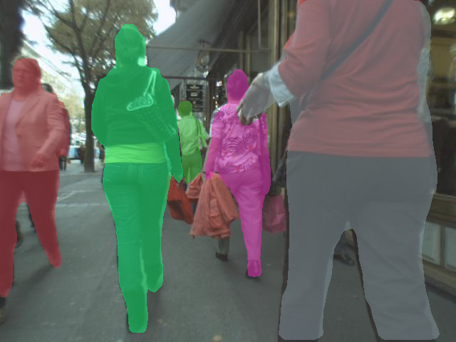
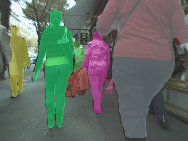
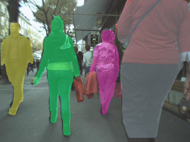
Figure 3: Sample MOTSNet predictions on a sub-sequence from the MOTS Challenge dataset.

5.5 MOTSNet on BDD100k

Since our MOTS training data generation pipeline can be directly ported to other datasets we also conducted experiments on the recently released BDD100k tracking dataset [54]. It comprises 61 sequences, for a total of $\sim 11$k frames and comes with bounding box based tracking annotations for a total of 8 classes (in our evaluation we focus only on cars and pedestrians, for compatibility with KITTI Synth and KITTI MOTS). We split the available data into training and validation sets of, respectively, 50 and 11 sequences, and generate segmentation masks for each annotated bounding box, again by using [39] augmented with a ResNeXt-101-32$\times$8d backbone. During data generation, the instance segmentation pipeline detected many object instances missing in the annotations, which is why we decided to provide ignore box annotations for detections with very high confidence but missing in the ground truth. Since there are only bounding-box based tracking annotations available, we present MOT rather than MOTS tracking scores. The results are listed in Tab. 4, comparing pooling strategies AveBox+Loss and AveMsk+Loss, again as a function of different pre-training settings. We again find that our proposed mask-pooling results compare favourable against the vanilla box-based pooling. While the improvement is small compared to the ImageNet-only pre-trained backbone, the Vistas pre-trained model benefits noticeably.

MOTSNet variant	Pre-training	MOTA	MOTP
AveBox+Loss	I	53.8	83.1
	I, M	56.9	83.9
AveMsk+Loss	I	53.9	83.1
	I, M	58.2	84.0

Table 4: MOT ablation results on the BDD100K dataset.

5.6 Ablations on Track Extraction

Here we analyze the importance of different cues in the payoff function used during inference (see Section 4.3): distance in the embedding space (Embedding), distance in time (Time) and signed intersection over union [46] (sIoU) between bounding boxes. As a basis, we take the best performing MOTSNet model from our experiments on KITTI MOTS, listed at the bottom of Table 2. This result was obtained by combining Embedding and Time, as in Eq. (C). As can be seen from differently configured results in Tab. 5, the embedding itself already serves as a good cue, and can be slightly improved on pedestrians when combined with information about proximity in time (with $0.1$ drop on cars), while outperforming sIoU. Figure 4 shows a visualization of the embedding vectors learned by this model.

sIoU	Embedding	Time	sMOTSA Car	sMOTSA Ped
✓	✗	✗	76.7	50.8
✗	✓	✗	78.2	54.4
✓	✗	✓	77.0	51.8
✗	✓	✓	78.1	54.6

Table 5: Ablation results on the KITTI MOTS dataset, using our best performing model from Tab. 2 when switching between different cues in the payoff function for inference.

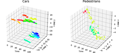
Figure 4: t-SNE visualization of the embedding vectors computed by the Tracking Head for sequence “0014” of KITTI MOTS. Points corresponding to detections of the same object have the same color.

6 Conclusions

In this work we addressed and provided two major contributions for the novel task of multi-object tracking and segmentation (MOTS). First, we introduced an automated pipeline for extracting high-quality training data from generic street-level videos to overcome the lack of MOTS training data, without time- and cost-intensive, manual annotation efforts. Data is generated by solving the linear assignment on a causal tracking graph, where instance segmentations per frame define the nodes, and optical-flow based compatibilities represent edges as connections over time. Our second major contribution is a deep-learning based MOTSNet architecture to be trained on MOTS data, exploiting a novel mask-pooling layer that guides the association process for detections based on instance segmentation masks. We provide exhaustive ablations for both, our novel training data generation process and our proposed MOTSNet. We improve over the previously best work [47] for the KITTI MOTS dataset (1.9%/7.5% for cars/pedestrians) and on MOTSChallenge (4.1% for pedestrians), respectively.

Appendix A CLEAR MOT and MOTS metrics

The CLEAR MOT metrics (including MOTA and MOTP) are first defined in [2] to evaluate Multi-Object Tracking systems. In order to compute MOTA and MOTP, a matching between the ground truth and predicted tracklets needs to be computed at each frame by solving a linear assignment problem. We will not repeat the details of this process, instead focusing on the way its outputs are used to compute the metrics. In particular, for each frame $t$, the matching process gives:

• the number of correctly matched boxes $\text{TP}_{t}$;

• the number of mismatched boxes $\text{IDS}_{t}$, i.e. the boxes belonging to a predicted tracklet that was matched to a different ground truth tracklet in the previous frame;

• the number of false positive boxes $\text{FP}_{t}$, i.e. the predicted boxes that are not matched to any ground truth;

• the number of ground truth boxes $\text{GT}_{t}$;

• the intersection over union $\text{IoU}_{t,i}$ between each correctly predicted box and its matching ground truth.

Given these, the metrics are defined as:

$$\text{MOTA}=\frac{\sum_{t}(\text{TP}_{t}-\text{FP}_{t}-\text{IDS}_{t})}{\sum_{t}\text{GT}_{t}}\,,$$

and

$$\text{MOTP}=\frac{\sum_{t,i}\text{IoU}_{t,i}}{\sum_{t}\text{TP}_{t}}\,.$$

The MOTS metrics [47] extend the CLEAR MOT metrics to the segmentation case. Their computation follows the overall procedure described above, with a couple of exceptions. First, box IoU is replaced with mask IoU. Second, the matching process is simplified by defining a ground truth and predicted segment to be matching if and only if their IoU is greater than 0.5. Different from the bounding box case, the segmentation masks are assumed to be non-overlapping, meaning that this criterion results in a unique matching without the need to solve a LAP. With these changes, and given the definitions above, the MOTS metrics are:

$$\text{MOTSA}=\frac{\sum_{t}(\text{TP}_{t}-\text{FP}_{t}-\text{IDS}_{t})}{\sum_{t}\text{GT}_{t}}\,,$$

$$\text{sMOTSA}=\frac{\sum_{t}(\sum_{i}\text{IoU}_{t,i}-\text{FP}_{t}-\text{IDS}_{t})}{\sum_{t}\text{GT}_{t}}\,,$$

and

$$\text{MOTSP}=\frac{\sum_{t,i}\text{IoU}_{t,i}}{\sum_{t}\text{TP}_{t}}\,.$$

Appendix B Hyper-parameters

B.1 Data Generation

In the data generation process, when constructing tracklets (see Sec. 3.2) we use the following parameters: $\tau_{0}=10\text{pix}$, $\tau_{1}=10\text{pix}$, $\tau_{2}=2$.

B.2 Network training

As mentioned in Sec. 5.2, all our trainings follow a linear learning rate schedule:

$$\text{lr}_{i}=\text{lr}_{0}\left(1-\frac{i}{\#\text{steps}}\right)\,,$$

where the initial learning rate $\text{lr}_{0}$ and total number of steps depend on the dataset and pre-training setting. The actual values, together with the per-GPU batch sizes $N_{w}$ are reported in Tab. 6. The loss weight parameter $\lambda$ in the first equation of Sec. 4.2 is fixed to $1$ in all experiments, except for the COCO pre-trained experiment on MOTSChallenge, where $\lambda=0.1$.

Dataset	Pre-training	$\text{lr}_{0}$	# epochs	$N_{w}$
KITTI Synth	I	0.02	20	12
	M	0.01	10	12
KITTI Synth, KITTI MOTS sequences	I	0.02	180	12
KITTI MOTS	I	0.02	180	12
	M, KS	0.01	90	12
BDD100k	all	0.02	100	10
MOTSChallenge	I	0.01	90	10
	C	0.02	180	10

Table 6: MOTSNet training hyperparameters for different datasets and pre-training settings.

Appendix C Signed Intersection over Union

Signed Intersection over Union, as defined in [46], extends standard intersection over union between bounding boxes, by providing meaningful values when the input boxes are not intersecting. Given two bounding boxes $\hat{\boldsymbol{b}}=(\hat{u}_{1},\hat{v}_{1},\hat{u}_{2},\hat{v}_{2})$ and $\boldsymbol{b}=(u_{1},v_{1},u_{2},v_{2})$, where $(u_{1},v_{1})$ and $(u_{2},v_{2})$ are the coordinates of a box’s top-left and bottom-right corners, respectively, the signed intersection over union $\text{sIoU}(\hat{\boldsymbol{b}},\boldsymbol{b})$ is:

• greater than 0 and equal to standard intersection over union when the boxes overlap;

• less than 0 when the boxes don’t overlap, and monotonically decreasing as their distance increases.

This is obtained by defining:

$$\text{sIoU}(\hat{\boldsymbol{b}},\boldsymbol{b})=\frac{|\hat{\boldsymbol{b}}\sqcap\boldsymbol{b}|_{\pm}}{|\hat{\boldsymbol{b}}|+|\boldsymbol{b}|-|\hat{\boldsymbol{b}}\sqcap\boldsymbol{b}|_{\pm}}\,,$$

where

$$\hat{\boldsymbol{b}}\sqcap\boldsymbol{b}=\left(\begin{array}[]{l}\max(\hat{u}_{1},u_{1})\\ \max(\hat{v}_{1},v_{1})\\ \min(\hat{u}_{2},u_{2})\\ \min(\hat{v}_{2},v_{2})\end{array}\right)$$

is an extended intersection operator, $|\boldsymbol{b}|$ denotes the area of $\boldsymbol{b}$, and

$$|\boldsymbol{b}|_{\pm}=\begin{cases}+|\boldsymbol{b}|&\text{if}\ u_{2}>u_{1}\land v_{2}>v_{1},\\ -|\boldsymbol{b}|&\text{otherwise},\end{cases}$$

is the “signed area” of $\boldsymbol{b}$.

Signed intersection over union is used in the ablation experiments of Sec. 5.6 as an additional term in the payoff function $\pi(\hat{s},s)$ as follows:

$$\pi(\hat{s},s) =-\pi^{*}(\hat{s},s)+\eta(s,\hat{s})\,,$$

$$\pi^{*}(\hat{s},s) =\text{sIoU}(\boldsymbol{b}_{s},\boldsymbol{b}_{\hat{s}})+\|a_{s}^{y_{s}}-a_{\hat{s}}^{y_{\hat{s}}}\|+\frac{|t_{s}-t_{\hat{s}}|}{N_{w}}\,,$$

where $\boldsymbol{b}_{s}$ denotes the bounding box of segment $s$.

Acknowledgements.

Idoia and Joan acknowledge financial support by the Spanish grant TIN2017-88709-R (MINECO/AEI/FEDER, UE).

References

- [1] Amanda Berg, Joakim Johnander, Flavie Durand de Gevigney, Jorgen Ahlberg, and Michael Felberg. Semi-automatic annotation of objects in visual-thermal video. In Proceedings of the IEEE International Conference on Computer Vision Workshops, 2019.
- [2] Keni Bernardin and Rainer Stiefelhagen. Evaluating multiple object tracking performance: the clear mot metrics. Journal on Image and Video Processing, page 1, 2008.
- [3] Luca Bertinetto, Jack Valmadre, Joao F Henriques, Andrea Vedaldi, and Philip HS Torr. Fully-convolutional siamese networks for object tracking. In Proceedings of the European Conference on Computer Vision, 2016.
- [4] Sergi Caelles, Kevis-Kokitsi Maninis, Jordi Pont-Tuset, Laura Leal-Taixe, Daniel Cremers, and Luc Van Gool. One-shot video object segmentation. In Proceedings of the IEEE Conference on Computer Vision and Pattern Recognition, 2017.
- [5] Sergi Caelles, Alberto Montes, Kevis-Kokitsi Maninis, Yuhua Chen, Luc Van Gool, Federico Perazzi, and Jordi Pont-Tuset. The 2018 davis challenge on video object segmentation. arXiv:1803.00557, 2018.
- [6] Liang-Chieh Chen, Yukun Zhu, George Papandreou, Florian Schroff, and Hartwig Adam. Encoder-decoder with atrous separable convolution for semantic image segmentation. In Proceedings of the European Conference on Computer Vision, September 2018.
- [7] Yuhua Chen, Jordi Pont-Tuset, Alberto Montes, and Luc Van Gool. Blazingly fast video object segmentation with pixel-wise metric learning. In Proceedings of the IEEE Conference on Computer Vision and Pattern Recognition, 2018.
- [8] Bowen Cheng, Maxwell D. Collins, Yukun Zhu, Ting Liu, Thomas S. Huang, Hartwig Adam, and Liang-Chieh Chen. Panoptic-deeplab. arXiv:1910.04751, 2019.
- [9] Marius Cordts, Mohamed Omran, Sebastian Ramos, Timo Rehfeld, Markus Enzweiler, Rodrigo Benenson, Uwe Franke, Stefan Roth, and Bernt Schiele. The Cityscapes dataset for semantic urban scene understanding. In Proceedings of the IEEE Conference on Computer Vision and Pattern Recognition, 2016.
- [10] A. Geiger, P. Lenz, C. Stiller, and R. Urtasun. Vision meets robotics: The KITTI dataset. The International Journal of Robotics Research, 2013.
- [11] Andreas Geiger, Philip Lenz, and Raquel Urtasun. Are we ready for autonomous driving? The kitti vision benchmark suite. In Proceedings of the IEEE Conference on Computer Vision and Pattern Recognition, 2012.
- [12] Kaiming He, Georgia Gkioxari, Piotr Dollár, and Ross B. Girshick. Mask R-CNN. In Proceedings of the IEEE International Conference on Computer Vision, 2017.
- [13] Kaiming He, Xiangyu Zhang, Shaoqing Ren, and Jian Sun. Deep residual learning for image recognition. arXiv:1512.03385, 2015.
- [14] Roberto Henschel, Laura Leal-Taixe, Daniel Cremers, and Bodo Rosenhahn. Fusion of head and full-body detectors for multi-object tracking. In Proceedings of the IEEE Conference on Computer Vision and Pattern Recognition Workshops, 2018.
- [15] Alexander Hermans, Lucas Beyer, and Bastian Leibe. In defense of the triplet loss for person re-identification. arXiv:1703.07737, 2017.
- [16] Junhwa Hur and Stefan Roth. Joint optical flow and temporally consistent semantic segmentation. arXiv:1607.07716, 2016.
- [17] Xiaojie Jin, Huaxin Xiao, Xiaohui Shen, Jimei Yang, Zhe Lin, Yunpeng Chen, Zequn Jie, Jiashi Feng, and Shuicheng Yan. Predicting scene parsing and motion dynamics in the future. In Neural Information Processing Systems, 2017.
- [18] Joakim Johnander, Martin Danelljan, Emil Brissman, Fahad Shahbaz Khan, and Michael Felsberg. A generative appearance model for end-to-end video object segmentation. In Proceedings of the IEEE Conference on Computer Vision and Pattern Recognition, 2019.
- [19] Margret Keuper, Siyu Tang, Bjorn Andres, Thomas Brox, and Bernt Schiele. Motion segmentation & multiple object tracking by correlation co-clustering. IEEE transactions on pattern analysis and machine intelligence, 2018.
- [20] Chanho Kim, Fuxin Li, Arridhana Ciptadi, and James M Rehg. Multiple hypothesis tracking revisited. In Proceedings of the IEEE International Conference on Computer Vision, 2015.
- [21] L. Leal-Taixé, A. Milan, I. Reid, S. Roth, and K. Schindler. MOTChallenge 2015: Towards a benchmark for multi-target tracking. arXiv:1504.01942, 2015.
- [22] Bo Li, Junjie Yan, Wei Wu, Zheng Zhu, and Xiaolin Hu. High performance visual tracking with siamese region proposal network. In Proceedings of the IEEE Conference on Computer Vision and Pattern Recognition, 2018.
- [23] F. Li, T. Kim, A. Humayun, D. Tsai, and J. M. Rehg. Video segmentation by tracking many figure-ground segments. In Proceedings of the IEEE International Conference on Computer Vision, 2013.
- [24] Tsung-Yi Lin, Michael Maire, Serge J. Belongie, Lubomir D. Bourdev, Ross B. Girshick, James Hays, Pietro Perona, Deva Ramanan, Piotr Dollár, and C. Lawrence Zitnick. Microsoft COCO: Common objects in context. In Proceedings of the European Conference on Computer Vision, 2014.
- [25] Tsung-Yi Lin, Piotr Dollár, Ross Girshick, Kaiming He, Bharath Hariharan, and Serge Belongie. Feature pyramid networks for object detection. In Proceedings of the IEEE conference on computer vision and pattern recognition, 2017.
- [26] Chen Long, Ai Haizhou, Zhuang Zijie, and Shang Chong. Real-time multiple people tracking with deeply learned candidate selection and person re-identification. In ICME, 2018.
- [27] Jonathan Long, Evan Shelhamer, and Trevor Darrell. Fully convolutional networks for semantic segmentation. In Proceedings of the IEEE Conference on Computer Vision and Pattern Recognition, 2015.
- [28] Pauline Luc, Camille Couprie, Yann LeCun, and Jakob Verbeek. Predicting future instance segmentations by forecasting convolutional features. In Proceedings of the European Conference on Computer Vision, 2018.
- [29] Jonathon Luiten, Philip Torr, and Bastian Leibe. Video instance segmentation 2019: A winning approach for combined detection, segmentation, classification and tracking. In Proceedings of the IEEE International Conference on Computer Vision Workshops, 2019.
- [30] Will Maddern, Geoffrey Pascoe, Chris Linegar, and Paul Newman. 1 year, 1000 km: The oxford robotcar dataset. International Journal of Robotics Research, 36(1):3–15, 2017.
- [31] Kevis-Kokitsi Maninis, Sergi Caelles, Jordi Pont-Tuset, and Luc Van Gool. Deep extreme cut: From extreme points to object segmentation. In Proceedings of the IEEE Conference on Computer Vision and Pattern Recognition, 2018.
- [32] Anton Milan, Laura Leal-Taixé, Ian D. Reid, Stefan Roth, and Konrad Schindler. MOT16: A benchmark for multi-object tracking. arXiv:1603.00831, 2016.
- [33] Gerhard Neuhold, Tobias Ollmann, Samuel Rota Bulò, and Peter Kontschieder. The mapillary vistas dataset for semantic understanding of street scenes. In Proceedings of the IEEE International Conference on Computer Vision, 2017.
- [34] Aljoša Ošep, Wolfgang Mehner, Markus Mathias, and Bastian Leibe. Combined image-and world-space tracking in traffic scenes. In Proceedings of the IEEE International Conference on Robotics and Automation, 2017.
- [35] Aljoša Ošep, Wolfgang Mehner, Paul Voigtlaender, and Bastian Leibe. Track, then decide: Category-agnostic vision-based multi-object tracking. In Proceedings of the IEEE International Conference on Robotics and Automation, 2018.
- [36] Aljoša Ošep, Paul Voigtlaender, Jonathon Luiten, Stefan Breuers, and Bastian Leibe. Towards large-scale video object mining. Proceedings of the ECCV 2018 Workshop on Interactive and Adaptive Learning in an Open World, 2018.
- [37] Federico Perazzi, Jordi Pont-Tuset, Brian McWilliams, Luc Van Gool, Markus Gross, and Alexander Sorkine-Hornung. A benchmark dataset and evaluation methodology for video object segmentation. In Proceedings of the IEEE Conference on Computer Vision and Pattern Recognition, 2016.
- [38] Jordi Pont-Tuset, Federico Perazzi, Sergi Caelles, Pablo Arbeláez, Alexander Sorkine-Hornung, and Luc Van Gool. The 2017 davis challenge on video object segmentation. arXiv:1704.00675, 2017.
- [39] Lorenzo Porzi, Samuel Rota Bulò, Aleksander Colovic, and Peter Kontschieder. Seamless scene segmentation. In Proceedings of the IEEE Conference on Computer Vision and Pattern Recognition, 2019.
- [40] A. Prest, C. Leistner, J. Civera, C. Schmid, and V. Ferrari. Learning object class detectors from weakly annotated video. In Proceedings of the IEEE Conference on Computer Vision and Pattern Recognition, 2012.
- [41] Jérôme Revaud, Philippe Weinzaepfel, Zaïd Harchaoui, and Cordelia Schmid. Epicflow: Edge-preserving interpolation of correspondences for optical flow. In Proceedings of the IEEE Conference on Computer Vision and Pattern Recognition, 2015.
- [42] Samuel Rota Bulò, Lorenzo Porzi, and Peter Kontschieder. In-place activated batchnorm for memory-optimized training of DNNs. In Proceedings of the IEEE Conference on Computer Vision and Pattern Recognition, 2018.
- [43] O. Russakovsky, J. Deng, H. Su, J. Krause, S. Satheesh, S. Ma, Z. Huang, A. Karphathy, A. Khosla, M. Bernstein, A. C. Berg, and L. Fei-Fei. Imagenet large scale visual recognition challenge. International Journal of Computer Vision, 2015.
- [44] Sarthak Sharma, Junaid Ahmed Ansari, J Krishna Murthy, and K Madhava Krishna. Beyond pixels: Leveraging geometry and shape cues for online multi-object tracking. In Proceedings of the IEEE International Conference on Robotics and Automation, 2018.
- [45] S. Shen. Accurate multiple view 3d reconstruction using patch-based stereo for large-scale scenes. IEEE Transactions on Image Processing, 22(5):1901–1914, 2013.
- [46] Andrea Simonelli, Samuel Rota Bulò, Lorenzo Porzi, Manuel López-Antequera, and Peter Kontschieder. Disentangling monocular 3d object detection. In Proceedings of the IEEE International Conference on Computer Vision, 2019.
- [47] Paul Voigtlaender, Michael Krause, Aljosa Osep, Jonathon Luiten, Berin Balachandar Gnana Sekar, Andreas Geiger, and Bastian Leibe. Mots: Multi-object tracking and segmentation. In Proceedings of the IEEE Conference on Computer Vision and Pattern Recognition, 2019.
- [48] Qiang Wang, Li Zhang, Luca Bertinetto, Weiming Hu, and Philip HS Torr. Fast online object tracking and segmentation: A unifying approach. In Proceedings of the IEEE Conference on Computer Vision and Pattern Recognition, 2019.
- [49] Longyin Wen, Dawei Du, Zhaowei Cai, Zhen Lei, Ming-Ching Chang, Honggang Qi, Jongwoo Lim, Ming-Hsuan Yang, and Siwei Lyu. Ua-detrac: A new benchmark and protocol for multi-object detection and tracking. arXiv:1511.04136, 2015.
- [50] Saining Xie, Ross Girshick, Piotr Dollár, Zhuowen Tu, and Kaiming He. Aggregated residual transformations for deep neural networks. In Proceedings of the IEEE Conference on Computer Vision and Pattern Recognition, 2017.
- [51] Ning Xu, Linjie Yang, Yuchen Fan, Dingcheng Yue, Yuchen Liang, Jianchao Yang, and Thomas Huang. Youtube-vos: A large-scale video object segmentation benchmark. arXiv:1809.03327, 2018.
- [52] Linjie Yang, Yuchen Fan, and Ning Xu. Video instance segmentation. arXiv:1905.04804, 2019.
- [53] Zhichao Yin, Trevor Darrell, and Fisher Yu. Hierarchical discrete distribution decomposition for match density estimation. In Proceedings of the IEEE International Conference on Computer Vision, 2019.
- [54] Fisher Yu, Wenqi Xian, Yingying Chen, Fangchen Liu, Mike Liao, Vashisht Madhavan, and Trevor Darrell. Bdd100k: A diverse driving video database with scalable annotation tooling. arXiv:1805.04687, 2018.
- [55] Idil Esen Zulfikar, Jonathon Luiten, and Bastian Leibe. Unovost: Unsupervised offline video object segmentation and tracking for the 2019 unsupervised davis challenge. In Proceedings of the 2019 DAVIS Challenge on Video Object Segmentation - CVPR Workshops, 2019.