Implementing a smooth exact penalty function
for general constrained nonlinear optimization

Abstract

We build upon Estrin et al. (2019a) to develop a general constrained nonlinear optimization algorithm based on a smooth penalty function proposed by Fletcher (1970, 1973b). Although Fletcher’s approach has historically been considered impractical, we show that the computational kernels required are no more expensive than those in other widely accepted methods for nonlinear optimization. The main kernel for evaluating the penalty function and its derivatives solves structured linear systems. When the matrices are available explicitly, we store a single factorization each iteration. Otherwise, we obtain a factorization-free optimization algorithm by solving each linear system iteratively. The penalty function shows promise in cases where the linear systems can be solved efficiently, e.g., PDE-constrained optimization problems when efficient preconditioners exist. We demonstrate the merits of the approach, and give numerical results on several PDE-constrained and standard test problems.

Dedicated to Roger Fletcher

1 Introduction

We consider a penalty-function approach for solving general constrained nonlinear optimization problems

(NP) $$\mathop{\hbox{minimize}}_{x\in\mathds{R}^{n}} f(x)$$

$$\mathop{\hbox{subject to}} c(x)=0 :\ y$$

$$\ell\leq x\leq u :\ z,$$

where $f:\mathds{R}^{n}\to\mathds{R}$ and $c:\mathds{R}^{n}\to\mathds{R}^{m}$ are smooth functions $(m\leq n)$, the $n$-vectors $\ell$ and $u$ provide (possibly infinite) bounds on $x$, and $y\in\mathds{R}^{m}$, $z\in\mathds{R}^{n}$ are Lagrange multipliers associated with the equality constraints and bounds respectively. Estrin et al. (2019a) describe factorization-based and factorization-free implementations of a smooth exact penalty method proposed by Fletcher (1970) to treat equality constraints. Here, we generalize our implementation to problems with both equality and bound constraints, and hence to problems with general inequality constraints.

Fletcher’s penalty function for equality constraints is the Lagrangian

(1.1) $$L(x,y)=f(x)-y^{T}\!c(x),$$

in which the vector $y=y_{\sigma}(x)$ is treated as a function of $x$ dependent on a parameter $\sigma>0$. Fletcher (1973b) proposes an extension to inequality constraints that exhibits nonsmoothness when constraint activities change. The penalty function (1.1) was long considered too costly for practical use (Bertsekas, 1975; Conn et al., 2000; Nocedal and Wright, 2006), and the nonsmooth extension to inequality constraints further impacted its practicality.

We demonstrate that a certain smooth extension of Fletcher’s penalty function yields a practical implementation for inequality-constrained optimization, by showing that the computational kernels are no more expensive than those in other widely accepted methods for nonlinear optimization, such as sequential quadratic programming.

The extended penalty function is exact because KKT points of (NP) are KKT points of the penalty problem for all values of $\sigma$ larger than a finite threshold $\sigma^{*}$. The main computational kernel for evaluating the penalty function and its derivatives is the solution of certain structured linear systems. We show how to solve the systems efficiently by factorizing a single matrix each iteration (if the matrix is available explicitly) and reusing the factors to evaluate the penalty function and its derivatives. We also provide a factorization-free implementation in which linear systems are solved iteratively. This makes the penalty function particularly applicable to certain problem classes such as PDE-constrained problems, where excellent preconditioners exist (e.g., those based on (Rees et al., 2010; Stoll and Wathen, 2012; Ridzal, 2013)); see Section 8.

The advantage of smooth exact penalty functions is that they lead to conceptually simpler algorithms compared to traditional methods for constrained problems. The original problem is replaced by a single smooth bound-constrained problem with a sufficiently large penalty parameter. This avoids complicated heuristics to trade-off primal and dual feasibility, and can avoid the need for primal feasibility restoration stages or composite-step methods. Further, because our penalty is smooth and we can compute a sufficiently accurate Hessian approximation, second-order methods with fast local convergence may be used.

Paper outline

We follow the structure of Estrin et al. (2019a). We introduce the penalty function in Section 2, and discuss its relationship with existing approaches in Section 3. We give the penalty function’s properties and derive an explicit threshold for the penalty parameter in Section 4. In Section 5 we show how to evaluate the penalty function and its derivatives efficiently. We discuss an extension to maintain linear constraints in Section 6. Practical considerations pertaining to the penalty function appear in Section 7. We apply the penalty approach to standard and PDE-constrained problems in Section 8, and discuss future research directions in Section 9.

2 The proposed penalty function

For (NP), we propose the penalty function

(2.1) $$\phi_{\sigma}(x):=f(x)-c(x)^{T}\!y_{\sigma}(x)=L(x,y_{\sigma}(x)),$$

where $y_{\sigma}(x)$ are Lagrange multiplier estimates defined with other items as

(2.2) $$y_{\sigma}(x) :=\textstyle{\mathop{\hbox{arg\,min}}_{y}}\ {\textstyle{\frac{1}{2}}}\|A(x)y-g(x)\|_{Q(x)}^{2}+\sigma c(x)^{T}\!y, g(x) :=\nabla f(x),$$

(2.3) $$A(x) :=\nabla c(x)=\begin{bmatrix}g_{1}(x)\ \cdots\ g_{m}(x)\end{bmatrix}, g_{i}(x) :=\nabla c_{i}(x),$$

(2.4) $$Y_{\sigma}(x) :=\nabla y_{\sigma}(x).$$

Note that $A$ and $Y_{\sigma}$ are $n$-by-$m$ matrices. We define an $n$-by-$n$ diagonal matrix $Q(x)=\textrm{diag}(q_{i}(x_{i}))$ with $\omega\in\mathds{R}_{+}^{n}$, $\omega<u-\ell$, and

(2.5) $${q_{i}(x_{i}):=\begin{cases}1&\mbox{if $\ell_{i}=-\infty$ and $u_{i}=\infty$},\\ {\textstyle{\frac{1}{2}}}(u_{i}-\ell_{i})-\tfrac{1}{4}\omega_{i}-\tfrac{1}{4\omega_{i}}\left(2x_{i}-u_{i}-\ell_{i}\right)^{2}&\mbox{if }|u_{i}+\ell_{i}-2x_{i}|\leq\omega_{i},\\ \min\{x_{i}-\ell_{i},u_{i}-x_{i}\}&\mbox{otherwise.}\end{cases}}$$

The diagonal of $Q(x)$ is a smooth approximation of $\min\{x-\ell,u-x\}$, and $\omega$ controls the smoothness. We use $\omega_{i}=\min\{1,{\textstyle{\frac{1}{2}}}(u_{i}-\ell_{i})\}$. Note that $Q(x)$ is nonnegative on $[\ell,u]$. We describe this function in more detail below.

We assume that (NP) satisfies the following conditions:

1. $f$ and $c$ are $\mathcal{C}_{3}$.

2. The linear independence constraint qualification (LICQ) is satisfied for stationary points and all $x$ satisfying $\ell<x<u$. LICQ is satisfied at $x$ if

   $$\left\{\nabla c_{i}(x),e_{j}\mid x_{j}\in\{\ell_{j},u_{j}\},\ i\in[m],\ j\in[n]\right\}$$

   is linearly independent, where $e_{j}$ is the $j$th column of the identity matrix, and $[n]:=\{1,2,\dots,n\}.$

3. Stationary points satisfy strict complementarity. If $(x^{*},y^{*},z^{*})$ is a stationary point, exactly one of $z^{*}_{j}$ and $\min\{x^{*}_{j}-\ell_{j},u_{j}-x^{*}_{j}\}$ is zero for all $j\in[n]$.

4. The problem is feasible. That is, there exists $x$ such that $\ell\leq x\leq u$ and $c(x)=0$, with $\ell_{j}<u_{j}$ for all $j\in[n]$. We assume fixed variables have been eliminated from the problem.

Assumption (A1) ensures that $\phi_{\sigma}$ has two continuous derivatives and is typical for smooth exact penalty functions (Bertsekas, 1982, Proposition 4.16). However, at most two derivatives of $f$ and $c$ are required to implement this penalty function in practice (see section 5.5). Assumption (A2) guarantees that $Y_{\sigma}(x)$ and $y_{\sigma}(x)$ are uniquely defined; (A3) provides additional regularity to ensure that the threshold penalty parameter $\sigma^{*}$ is well defined.

The basis of our approach is to solve

(PP) $$\mathop{\hbox{minimize}}_{x\in\mathds{R}^{n}}\quad\phi_{\sigma}(x)\quad\mathop{\hbox{subject to}}\quad\ell\leq x\leq u:\ z$$

instead of (NP). We purposely set $z$ to be the Lagrange multiplier for the bound constraints of both (NP) and (PP) because, as we show, they are equal at a solution.

2.1 The scaling matrix

The diagonal entries of the scaling matrix $Q(x)$ are smooth approximations of the complementarity function $\min\{x-\ell,u-x\}$ (Chen, 2000). Fig. 1 plots $q(x)$ with finite $\ell$ and $u$.

[mode=buildnew,page=1,scale=1]illustrations

Figure 1: Plot of $q(x)$, a smooth approximation of $\min\{x-\ell,u-x\}$.

The definition of $y_{\sigma}(x)$ (2.2) can be interpreted as a smooth approximation of the complementarity conditions in the first-order KKT conditions (4.2d)–(4.2f) below. The role of $Q(x)$ is therefore to ensure that the partial derivatives of the Lagrangian corresponding to indices of inactive bounds are zero. Similar smoothing strategies can be found in the complementarity constraint literature (Anitescu, 2000; Leyffer, 2006).

For $x\in\mathds{R}$, the derivative of $q(x)$ is

(2.6) $$q^{\prime}(x)=\begin{cases}0&\mbox{if $\ell=-\infty$ and $u=\infty$,}\\ -\tfrac{1}{\omega}\left(2x+u-\ell\right)&\mbox{if $|u+\ell-2x|\leq\omega$,}\\ 1&\mbox{if $x-\ell<u-x$,}\\ {-1}&\mbox{if $x-\ell>u-x$.}\end{cases}$$

Note that the cases in (2.6) are not mutually exclusive, and should be checked top to bottom until a case is satisfied. The choice of $q(x)$ is not unique because any smooth concave function that is zero at $x_{j}\in\{\ell_{j},u_{j}\}$ works in our framework. For instance, if $u_{j}-\ell_{j}$ is large, we could use a smooth approximation of $\min\{x_{j}-\ell_{j},u_{j}-x_{j},1\}$ to avoid numerical issues that can arise if $x$ is far from its bounds.

2.2 Notation

Denote $x^{*}$ as a local stationary point of (NP), with corresponding dual solutions $y^{*}$ and $z^{*}$. At $x^{*}$, define the set of active bounds as

(2.7) $$\mathcal{A}(x^{*}):=\{j\mid x_{j}\in\{\ell_{j},u_{j}\}\},$$

and define the critical cones $C_{\phi}(x^{*},z^{*})$ and $C(x^{*},z^{*})$ as

(2.8d) $$\mathcal{C}_{\phi}(x^{*},z^{*}) :=\left\{p\,\middle|\begin{array}[]{cl}p_{j}=0&\mbox{if }z^{*}_{j}\neq 0\\ p_{j}\geq 0&\mbox{if }x^{*}_{j}=\ell_{j}\\ p_{j}\leq 0&\mbox{if }x^{*}_{j}=u_{j}\end{array}\right\},$$

(2.8e) $$\mathcal{C}(x^{*},z^{*}) :=\left\{p\in\mathcal{C}_{\phi}(x^{*},z^{*})\,\middle|\,A(x^{*})^{T}\!p=0\right\}.$$

Observe that by (A3), $\mathcal{C}_{\phi}(x^{*},z^{*})=\left\{p\mid p_{j}=0\mbox{ if }z^{*}_{j}\neq 0\right\}$, so $p\in\mathcal{C}_{\phi}(x^{*},z^{*})$ if and only if $p=Q(x^{*})^{1/2}{\bar{p\mkern 2.0mu}\mkern-2.0mu}{}$ for some ${\bar{p\mkern 2.0mu}\mkern-2.0mu}{}\in\mathds{R}^{n}$.

Let $g(x)=\nabla f(x)$, $H(x)=\nabla^{2}f(x)$, $g_{i}(x)=\nabla c_{i}(x)$, $H_{i}(x)=\nabla^{2}c_{i}(x)$, and define

(2.9) $$g_{\scriptscriptstyle L}(x,y) :=g(x)-A(x)y,\qquad g_{\sigma}(x) :=g_{\scriptscriptstyle L}(x,y_{\sigma}(x)),$$

$$H_{\scriptscriptstyle L}(x,y) :=H(x)-\sum_{i=1}^{m}y_{i}H_{i}(x),\qquad H_{\sigma}(x) :=H_{\scriptscriptstyle L}(x,y_{\sigma}(x))$$

as the gradient and Hessian of $L$ at $(x,y)$ or $(x,y_{\sigma}(x))$. We define the matrix operators

$$R(x,v) :=\nabla_{x}[Q(x)v]=\nabla_{x}\begin{bmatrix}q_{1}(x_{1})v_{1}\\ \vdots\\ q_{n}(x_{n})v_{n}\end{bmatrix}=\operatorname{diag}\left(\begin{bmatrix}q_{1}^{\prime}(x_{1})v_{1}\\ \vdots\\ q_{n}^{\prime}(x_{n})v_{n}\end{bmatrix}\right),$$

$$S(x,v) :=\nabla_{x}[A(x)^{T}\!v]=\nabla_{x}\begin{bmatrix}g_{1}(x)^{T}v\\ \vdots\\ g_{m}(x)^{T}v\end{bmatrix}=\begin{bmatrix}v^{T}H_{1}(x)\\ \vdots\\ v^{T}H_{m}(x)\end{bmatrix},$$

$$T(x,w) :=\nabla_{x}[A(x)w]=\nabla_{x}\left[\sum_{i=1}^{m}w_{i}g_{i}(x)\right]=\sum_{i=1}^{m}w_{i}H_{i}(x),$$

where $v\in\mathds{R}^{n}$, $w\in\mathds{R}^{m}$, and $T$ is a symmetric matrix. The operation of multiplying the adjoint of $S$ with a vector $w$ is described by

$$S(x,v)^{T}w =\left[\sum_{i=1}^{m}w_{i}H_{i}(x)\right]v=T(x,w)v=T(x,w)^{T}v\,.$$

If $A_{Q}(x)=Q(x)^{1/2}A(x)$ has full rank $m$, the operators

(2.10) $$P(x):=A_{Q}(x)\big{(}A_{Q}(x)^{T}\!A_{Q}(x)\big{)}^{-1}A_{Q}(x)^{T}\text{and}{\bar{P\mkern 5.0mu}\mkern-5.0mu}{}(x):=I-P(x)$$

define orthogonal projectors onto $\mathop{\hbox{\rm range}}(A_{Q}(x))$ and its complement respectively. More generally, for a matrix $M$, we define $P_{M}$ and ${\bar{P\mkern 5.0mu}\mkern-5.0mu}{}_{M}$ as the orthogonal projectors onto $\mathop{\hbox{\rm range}}(M)$ and $\mathop{\hbox{\rm null}}(M)$ respectively.

Unless otherwise indicated, $\|\cdot\|$ is the 2-norm for vectors and matrices. For $M$ positive definite, $\|u\|^{2}_{M}=u^{T}\!Mu$ is the energy-norm. For square matrices $M$, define $\lambda_{\max}(M)$ as its largest eigenvalue. Define $\mathbbm{1}$ as the vector of all ones of size dictated by the context.

3 Related work on penalty functions for inequality constraints

Penalty functions have long been used to solve constrained problems by replacing constraints with functions that penalize infeasibility. Estrin et al. (2019a, §1.1) give an overview of other smooth exact penalty methods for equality constrained optimization and their relation to (PP). A more detailed overview is given by Di Pillo and Grippo (1984), Conn et al. (2000), and Nocedal and Wright (2006).

When $\ell=0$ and $u=\infty$, Fletcher (1973b) proposes the penalty function

$$\psi_{\sigma}(x) :=f(x)-c(x)^{T}\!y_{\sigma}(x)-z_{\sigma}(x)^{T}\!x,$$

$$y_{\sigma}(x),z_{\sigma}(x) :=\mathop{\hbox{arg\,min}}_{\{y\in\mathds{R}^{m},\,z\geq 0\}}{\textstyle{\frac{1}{2}}}\|A(x)y+z-g(x)\|_{2}^{2}+\sigma c(x)^{T}\!y$$

and minimizes $\psi_{\sigma}$ unconstrained. Although $\psi_{\sigma}$ is exact and continuous, it is nonsmooth because of the bound constraints on $z$: active-set changes on those bounds correspond to non-differentiable points for $\psi_{\sigma}$. Solving the penalty problem requires a method for nonsmooth problems, and Maratos (1978) observes that nonsmooth merit functions may result in slow convergence.

Since Fletcher (1973a), there has been significant work on smooth exact penalty methods that handle inequality constraints (Di Pillo and Grippo, 1984, 1985; Boggs et al., 1992; Zavala and Anitescu, 2014). Many approaches replace the inequality constraints with equalities using squared slacks (Bertsekas, 1982), at which point the equality constrained problem is solved via a smooth exact penalty approach. (This is one approach for deriving $\phi_{\sigma}$ and (2.2); however, it is also possible to derive it directly from the first-order KKT conditions.) The penalty function in these cases is the augmented Lagrangian, which either keeps the dual variables explicit and penalizes the gradient of the Lagrangian (Zavala and Anitescu, 2014), or expresses the dual variables as a function of $x$ (Di Pillo and Grippo, 1984). Our penalty function (2.1) takes the latter approach but defines this parametrization differently from previous approaches; rather than introducing additional dual variables for the bounds in (2.2), we change the norm of the least-squares problem according to the distance from the bounds, to approximate the complementarity conditions of first-order KKT points.

4 Properties of the penalty function

In this section, we show how $\phi_{\sigma}(x)$ naturally expresses the optimality conditions of (NP). We also give explicit expressions for the threshold value of the penalty parameter $\sigma$.

As in (Estrin et al., 2019a), the gradient and Hessian of $\phi_{\sigma}$ may be written as

(4.1a) $$\nabla\phi_{\sigma}(x) =g_{\sigma}(x)-Y_{\sigma}(x)c(x),$$

(4.1b) $$\nabla^{2}\phi_{\sigma}(x) =H_{\sigma}(x)-A(x)Y_{\sigma}(x)^{T}-Y_{\sigma}(x)A(x)^{T}-\nabla_{x}\left[Y_{\sigma}(x)c\right],$$

where the last term $\nabla_{x}[Y_{\sigma}(x)c]$ purposely drops the argument on $c$ to emphasize that this gradient is made on the product $Y_{\sigma}(x)c$ with $c:=c(x)$ held fixed. This term involves third derivatives of $f$ and $c$, and as we shall see, it is convenient and computationally efficient to ignore it. We leave it unexpanded.

The penalty function $\phi_{\sigma}$ is closely related to the (partial) Lagrangian (1.1). To make this connection clear, we define the Karush-Kuhn-Tucker (KKT) optimality conditions for (NP) in terms of those of (PP). From the definition of $\phi_{\sigma}$ and $y_{\sigma}$ and (4.1), we have the following definition.

Definition 4.1 (First-order KKT points of (NP)).

The point $(x^{*},z^{*})$ is a first-order KKT point of (NP) if for any $\sigma\geq 0$ the following hold:

(4.2a) $$\ell\leq x^{*} \leq u,$$

(4.2b) $$c(x^{*}) =0,$$

(4.2c) $$\nabla\phi_{\sigma}(x^{*}) =z^{*},$$

(4.2d) $$z^{*}_{j} =0,\qquad\mbox{if }j\notin\mathcal{A}(x^{*}),$$

(4.2e) $$z^{*}_{j} \geq 0,\qquad\mbox{if }x^{*}_{j}=\ell_{j},$$

(4.2f) $$z^{*}_{j} \leq 0,\qquad\mbox{if }x^{*}_{j}=u_{j}.$$

Then $y^{*}:=y_{\sigma}(x^{*})$ is the Lagrange multiplier of (NP) associated with $x^{*}$. Note that by (A3), inequalities (4.2e) and (4.2f) are strict.

Remark 4.2.

If (4.2) holds for some $\sigma\geq 0$, it necessarily holds for all $\sigma\geq 0$ because $c(x^{*})=0$. Also, the point $(x^{*},z^{*})$ is a first-order KKT point of (PP) if for any $\sigma\geq 0$, (4.2a) and (4.2c)–(4.2f) hold.

Definition 4.3 (Second-order KKT point of (NP)).

The first-order KKT point $(x^{*},z^{*})$ satisfies the second-order necessary KKT condition for (NP) if for any $\sigma\geq 0$,

(4.3) $$p^{T}\nabla^{2}\phi_{\sigma}(x^{*})p\geq 0\quad\hbox{for all $p\in\mathcal{C}(x^{*},z^{*})$. }$$

Condition (4.3) is sufficient if the inequality is strict.

Remark 4.4.

If $(x^{*},z^{*})$ is a first-order KKT point for (PP), then replacing $\mathcal{C}(x^{*},z^{*})$ by $\mathcal{C}_{\phi}(x^{*},z^{*})$ in Definition 4.3 corresponds to second-order KKT points of (PP).

The second-order KKT condition says that at a second-order KKT point of (PP), $\phi_{\sigma}$ has nonnegative curvature along directions in the critical cone $\mathcal{C}_{\phi}(x^{*},z^{*})$. We now show that at $x^{*}$, increasing $\sigma$ increases curvature only along the normal cone to the equality constraints. We derive a threshold value for $\sigma$ beyond which that $\phi_{\sigma}$ has nonnegative curvature even when $A(x^{*})^{T}\!p\neq 0$, as well as a condition on $\sigma$ that ensures that stationary points of (PP) are primal feasible. For a given first- or second-order KKT triple $(x^{*},y^{*},z^{*})$ of (NP), we define

(4.4) $$\sigma^{*}:={\textstyle{\frac{1}{2}}}\lambda^{+}_{\max}\left(P(x^{*})Q(x^{*})^{1/2}H_{\scriptscriptstyle L}(x^{*},y^{*})Q(x^{*})^{1/2}P(x^{*})\right),$$

where $\lambda^{+}_{\max}(\cdot)=\max\{\lambda_{\max}(\cdot),0\}$. The following lemmas are similar to those of Estrin et al. (2019a). Indeed, if the bounds are absent then $Q(x)=I$ and we recover the same results as in Estrin et al. (2019a).

Lemma 4.5.

If $c(x)\in\mathop{\hbox{\rm range}}\left(A(x)^{T}\!Q(x)\right)$, then $y_{\sigma}(x)$ satisfies (4.5) $$A(x)^{T}\!Q(x)A(x)y_{\sigma}(x)=A(x)^{T}\!Q(x)g(x)-\sigma c(x).$$ Furthermore, if $Q(x)A(x)$ has full rank, then (4.6) $\displaystyle A(x)^{T}\!Q(x)A(x)Y_{\sigma}(x)^{T}\!$ $\displaystyle\qquad=A(x)^{T}\!\left[Q(x)H_{\sigma}(x)-\sigma I+R(x,g_{\sigma}(x))\right]+S(x,Q(x)g_{\sigma}(x)).$

Proof 4.6.

For any $x$, the necessary and sufficient optimality conditions for (2.2) give (4.5). For brevity, let everything be evaluated at the same point $x$ and drop the argument $x$ from all operators. By differentiating both sides of (4.5), we obtain

$$S(QAy_{\sigma})+A^{T}\!\left[R(Ay_{\sigma})+QT(y_{\sigma})+QAY_{\sigma}^{T}\right]=S(Qg)+A^{T}\!\left[R(g)+QH-\sigma I\right].$$

The derivative exists because $y_{\sigma}(x)$ is well-defined in a neighbourhood of $x$ if $Q(x)A(x)$ is full-rank. By rearranging the above and using definitions (2.9), we obtain (4.6).

Theorem 4.7 (Threshold penalty value).

Suppose $(\bar{x},{\bar{z\mkern 2.8mu}\mkern-2.8mu}{})$ is a first-order KKT point for (PP) with $Q(\bar{x})^{1/2}A(\bar{x})$ full-rank, and let $(x^{*},y^{*},z^{*})$ be a second-order necessary KKT point for (NP). Then (4.7a) $\displaystyle\sigma>\|A(\bar{x})^{T}Q(\bar{x})Y_{\sigma}(\bar{x})\|$ $\displaystyle\quad\Longrightarrow\quad c(\bar{x})=0;$ (4.7b) $\displaystyle p^{T}\nabla^{2}\phi_{\sigma}(x^{*})p\geq 0\text{for all}p\in\mathcal{C}_{\phi}(x^{*},z^{*})$ $\displaystyle\quad\!\Longleftrightarrow\quad\sigma\geq\bar{\sigma},$ where $\bar{\sigma}={\textstyle{\frac{1}{2}}}\lambda_{\max}\left(P(x^{*})Q(x^{*})^{1/2}H_{\scriptscriptstyle L}(x^{*},y^{*})Q(x^{*})^{1/2}P(x^{*})\right)$ is defined in (4.4). The consequence of (4.7a) is that $\bar{x}$ is a first-order KKT point for (NP). If $x^{*}$ is second-order sufficient, the inequalities in (4.7b) hold strictly. Observe that $\sigma^{*}=\max\{\bar{\sigma},0\}$.

Proof 4.8.

Proof of (4.7a): By (4.2c)–(4.2f), $Q(\bar{x})\nabla\phi_{\sigma}(\bar{x})=0$, so that

$$Q(\bar{x})g(\bar{x})=Q(\bar{x})A(\bar{x})y_{\sigma}(\bar{x})+Q(\bar{x})Y_{\sigma}(\bar{x})c(\bar{x}).$$

Substituting (4.5) evaluated at $\bar{x}$ into this equation yields, after simplifying,

$$A(\bar{x})^{T}\!Q(\bar{x})Y_{\sigma}(\bar{x})c(\bar{x})=\sigma c(\bar{x}).$$

Taking norms of both sides and using the triangle inequality gives the inequality $\sigma\|c(\bar{x})\|\leq\|A(\bar{x})^{T}Q(\bar{x})Y_{\sigma}(\bar{x})\|\,\|c(\bar{x})\|$, which implies that $c(\bar{x})=0$.

Proof of (4.7b): Because $x^{*}$ satisfies first-order conditions (4.2), we have $y^{*}=y_{\sigma}(x^{*})$ and $Q(x^{*})g_{\sigma}(x^{*})=0$, independently of $\sigma$. Therefore $S(x^{*},Q(x^{*})g_{\sigma}(x^{*}))=0$. We drop the arguments from operators that take $x$ as input and assume that they are all evaluated at $x^{*}$. By premultiplying (4.6) by $(A_{Q}^{\dagger})^{T}=Q^{1/2}A(A^{T}\!QA)^{-1}$ and postmultiplying by $Q^{1/2}$, using $H_{\scriptscriptstyle L}(x^{*},y^{*})=H_{\sigma}$, and the definition of $P:=P(x^{*})$, we have

(4.8) $$Q^{1/2}AY_{\sigma}^{T}Q^{1/2} =(A_{Q}^{\dagger})^{T}A^{T}(QH_{\scriptscriptstyle L}(x^{*},y^{*})Q^{1/2}-\sigma I+R(g_{\sigma}))Q^{1/2}$$

(4.9) $$=PQ^{1/2}H_{\scriptscriptstyle L}(x^{*},y^{*})Q^{1/2}-\sigma P+(A_{Q}^{\dagger})^{T}AR(g_{\sigma})Q^{1/2}$$

Observe that if $p\in\mathcal{C}_{\phi}(x^{*},z^{*})$, then $p=Q^{1/2}{\bar{p\mkern 2.0mu}\mkern-2.0mu}{}$ for some ${\bar{p\mkern 2.0mu}\mkern-2.0mu}{}\in\mathcal{C}_{\phi}(x^{*},z^{*})$. Because $Q^{1/2}g_{\sigma}=0$, we have $R(g_{\sigma})Q^{1/2}=0$. Therefore using (4.1b), (4.9), $c(x^{*})=0$, and the relation $P+{\bar{P\mkern 5.0mu}\mkern-5.0mu}{}=I$, we have

$$p^{T}\nabla^{2}\phi_{\sigma}(x^{*})p\geq 0 \Leftrightarrow{\bar{p\mkern 2.0mu}\mkern-2.0mu}{}^{T}Q^{1/2}\left(H_{\sigma}-AY_{\sigma}^{T}\!-Y_{\sigma}A^{T}\right)Q^{1/2}{\bar{p\mkern 2.0mu}\mkern-2.0mu}{}\geq 0$$

$$\Leftrightarrow{\bar{p\mkern 2.0mu}\mkern-2.0mu}{}^{T}\left(Q^{1/2}H_{\sigma}Q^{1/2}-PQ^{1/2}H_{\sigma}Q^{1/2}-Q^{1/2}H_{\sigma}Q^{1/2}P+2\sigma P\right){\bar{p\mkern 2.0mu}\mkern-2.0mu}{}$$

$$\Leftrightarrow{\bar{p\mkern 2.0mu}\mkern-2.0mu}{}^{T}\left({\bar{P\mkern 5.0mu}\mkern-5.0mu}{}Q^{1/2}H_{\sigma}Q^{1/2}{\bar{P\mkern 5.0mu}\mkern-5.0mu}{}-PQ^{1/2}H_{\sigma}Q^{1/2}P+2\sigma P\right){\bar{p\mkern 2.0mu}\mkern-2.0mu}{}\geq 0.$$

Now, because ${\bar{P\mkern 5.0mu}\mkern-5.0mu}{}{\bar{p\mkern 2.0mu}\mkern-2.0mu}{}\in\mathop{\hbox{\rm null}}(A^{T}Q^{1/2})$ implies that $Q^{1/2}{\bar{P\mkern 5.0mu}\mkern-5.0mu}{}{\bar{p\mkern 2.0mu}\mkern-2.0mu}{}\in\mathcal{C}(x^{*},z^{*})$, the first term above is nonnegative according to Definition 4.3. It follows that $\sigma$ must be sufficiently large that $2\sigma P-PQ^{1/2}H_{\scriptscriptstyle L}(x^{*},y^{*})Q^{1/2}P\succeq 0$, which is equivalent to $\sigma\geq\bar{\sigma}$.

As in Estrin et al. (2019a, Theorem 4), (4.7b) shows that if $x^{*}$ is a second-order KKT point of (NP), there exists a threshold value $\bar{\sigma}$ beyond which $x^{*}$ is also a second-order KKT point of (PP). As penalty parameters are typically nonnegative, we treat $\sigma^{*}=\max\{\bar{\sigma},0\}$ as the threshold. Note that this result does not preclude the possibility that there exist minimizers of the penalty function—for any value of $\sigma$—that are not minimizers of (NP). However, these are rarely encountered in practice. Further, we can add a quadratic penalty term that, under certain conditions, ensures that KKT points of (PP) are feasible for (NP) (Estrin et al., 2019a, §3.3).

5 Evaluating the penalty function

The main challenge in evaluating $\phi_{\sigma}$ and its gradient is the solution of the shifted weighted-least-squares problem (2.2) needed to compute $y_{\sigma}(x)$, and computation of the gradient $Y_{\sigma}(x)$. We show below that it is possible to compute matrix-vector products $Y_{\sigma}(x)v$ and $Y_{\sigma}(x)^{T}\!u$ by solving structured linear systems involving the same matrix. We show that this linear system may be either symmetric or unsymmetric, and discuss the tradeoffs between both approaches. In either case, if direct methods are to be used, only a single factorization that defines the solution (2.2) is required for all products.

For this section, it is convenient to drop the arguments on various functions and assume they are all evaluated at a point $x$ for some parameter $\sigma$. For example, $y_{\sigma}=y_{\sigma}(x),\ A=A(x),\ Y_{\sigma}=Y_{\sigma}(x),\ H_{\sigma}=H_{\sigma}(x),\ S_{\sigma}=S(x,Q(x)g_{\sigma}(x)),R_{\sigma}=R(x,g_{\sigma}(x))$, etc. We express (4.6) using the shorthand notation

(5.1) $$A^{T}\!QAY_{\sigma}^{T}=A^{T}(QH_{\sigma}-\sigma I+R_{\sigma})+S_{\sigma}.$$

We first describe how to compute products $Y_{\sigma}u$ and $Y_{\sigma}^{T}\!v$, then how to put those pieces together to evaluate the penalty function and its derivatives.

Every quantity of interest can be computed by solving a symmetric or unsymmetric linear system and combining the solution with the derivatives of the problem data. Typically it is preferable to solve symmetric systems; however, we find that additional Jacobian products are then needed. The additional cost may be negligible, but this matter becomes application-dependent. We therefore present both options, beginning with the symmetric case.

There are many ways to construct the right-hand sides of the linear systems presented below. One consideration is that inversions with the diagonal matrix $Q^{1/2}$ should be avoided—even though the diagonal of $Q$ will be assumed strictly positive because of the use of an interior method (see Section 7), numerical difficulties may arise near the boundary of the feasible set if $Q^{1/2}$ contains small entries and is inverted.

5.1 Computing $\mathbf{Y_{\sigma}u}$

It follows from (5.1) that for a given $m$-vector $u$,

$$Y_{\sigma}u =(H_{\sigma}Q-\sigma I+R_{\sigma})A(A^{T}\!QA)^{-1}u+S_{\sigma}^{T}\!(A^{T}\!QA)^{-1}u.$$

Let $w=-(A^{T}QA)^{-1}u$ and $v=-Q^{1/2}Aw$, so that $v$ and $w$ are the solution of the symmetric linear system

(5.2) $$\begin{bmatrix}I&Q^{1/2}A\\ A^{T}Q^{1/2}\end{bmatrix}\begin{bmatrix}v\\ w\end{bmatrix}=\begin{bmatrix}0\\ u\end{bmatrix}.$$

Then $Y_{\sigma}u=H_{\sigma}Q^{1/2}v+(\sigma I-R_{\sigma})Aw-S_{\sigma}^{T}\!w$. Algorithm 1 formalizes this process.

Algorithm 1 Computing the matrix-vector product $Y_{\sigma}u$

1:$(v,w)\leftarrow\hbox{solution of~{}\eqref{eq:aug-Yu-sym}}$

2:return $H_{\sigma}Q^{1/2}v+(\sigma I-R_{\sigma})Aw-S_{\sigma}^{T}\!w$

5.2 Computing $\mathbf{Y_{\sigma}^{T}\!v}$

Again from (5.1), multiplying both sides by $v$ gives

$$Y_{\sigma}^{T}\!v =(A^{T}\!QA)^{-1}A^{T}(QH_{\sigma}-\sigma I+R_{\sigma})v+(A^{T}\!QA)^{-1}S_{\sigma}v.$$

The product $u=Y_{\sigma}^{T}\!v$ is part of the solution of the system

(5.3) $$\begin{bmatrix}I&Q^{1/2}A\\ A^{T}Q^{1/2}\end{bmatrix}\begin{bmatrix}r\\ u\end{bmatrix}=\begin{bmatrix}Q^{1/2}H_{\sigma}v\\ A^{T}\!(\sigma I-R_{\sigma})v-S_{\sigma}v\end{bmatrix}.$$

Algorithm 2 formalizes the process.

Algorithm 2 Computing the matrix-vector product $Y_{\sigma}^{T}\!v$

1:Evaluate $Q^{1/2}H_{\sigma}v$ and $A^{T}\!(\sigma I+R_{\sigma})v-S_{\sigma}v$

2:$(r,u)\leftarrow\hbox{solution of~{}\eqref{eq:aug-YTv-sym}}$

3:return $u$

5.3 Unsymmetric linear system

We briefly comment on how to use unsymmetric systems in place of (5.2) and (5.3). We can compute products of the form $Y_{\sigma}u=(H_{\sigma}-\sigma I+R_{\sigma}){\bar{v\mkern 3.0mu}\mkern-3.0mu}{}-S_{\sigma}^{T}\!w$ (where $w=-(A^{T}QA)^{-1}u$ and ${\bar{v\mkern 3.0mu}\mkern-3.0mu}{}=-Aw$), and products $u=Y_{\sigma}^{T}\!v$ by solving the respective linear systems:

(5.4) $$\begin{bmatrix}I&A\\ A^{T}Q\end{bmatrix}\begin{bmatrix}{\bar{v\mkern 3.0mu}\mkern-3.0mu}{}\\ w\end{bmatrix}=\begin{bmatrix}0\\ u\end{bmatrix}\text{and}\begin{bmatrix}I&QA\\ A^{T}\end{bmatrix}\begin{bmatrix}{\bar{r\mkern 3.0mu}\mkern-3.0mu}{}\\ u\end{bmatrix}=\begin{bmatrix}(QH_{\sigma}-\sigma I-R_{\sigma})v\\ -S_{\sigma}v\end{bmatrix}.$$

Algorithms 1 and 2 can then be appropriately modified to use the above linear systems.

5.4 Computing multipliers and first derivatives

The multiplier estimates $y_{\sigma}$ and Lagrangian gradient can be obtained from one of the following linear systems:

(5.5) $$\begin{bmatrix}I&Q^{1/2}A\\ A^{T}Q^{1/2}\end{bmatrix}\begin{bmatrix}d\\ y_{\sigma}\end{bmatrix}=\begin{bmatrix}Q^{1/2}g\\ \sigma c\end{bmatrix}\qquad\mbox{or}\qquad\begin{bmatrix}I&A\\ A^{T}Q\end{bmatrix}\begin{bmatrix}g_{\sigma}\\ y_{\sigma}\end{bmatrix}=\begin{bmatrix}g\\ \sigma c\end{bmatrix}.$$

Observe that in the unsymmetric case we obtain $g_{\sigma}$ immediately. The symmetric system yields $d=Q^{1/2}g_{\sigma}$. As noted earlier, computing $g_{\sigma}\leftarrow Q^{-1/2}d$ may amplify errors when the diagonal entries of $Q$ are approaching zero. An alternative would be to compute $g_{\sigma}\leftarrow g-Ay_{\sigma}$, which costs an extra Jacobian product.

The penalty gradient $\nabla\phi_{\sigma}=g_{\sigma}-Y_{\sigma}c$ can then be computed using $g_{\sigma}$ and computing $Y_{\sigma}c$ via Algorithm 1 or its unsymmetric variant.

5.5 Computing second derivatives

We approximate $\nabla^{2}\phi_{\sigma}$ from (4.1b) using the same approaches as Estrin et al. (2019a):

(5.6a) $$\nabla^{2}\phi_{\sigma} \approx B_{1}:=H_{\sigma}-AY_{\sigma}^{T}-Y_{\sigma}A^{T}$$

$$\phantom{\approx B_{1}:}=H_{\sigma}-\widetilde{P}(QH_{\sigma}+R_{\sigma}-\sigma I)-(H_{\sigma}Q+R_{\sigma}-\sigma I)\widetilde{P}$$

$$\phantom{\approx B_{1}:}\qquad-A(A^{T}\!QA)^{-1}S_{\sigma}-S_{\sigma}^{T}(A^{T}\!QA)^{-1}A$$

(5.6b) $$\approx B_{2}:=H_{\sigma}-\widetilde{P}(QH_{\sigma}+R_{\sigma}-\sigma I)-(H_{\sigma}Q+R_{\sigma}-\sigma I)\widetilde{P},$$

where $\widetilde{P}=A(A^{T}\!QA)^{-1}A$. The first approximation drops the third derivative term $\nabla[Y_{\sigma}c]$ in (4.1b), while the second approximation drops the term $S_{\sigma}(x,Qg_{\sigma})$, because those terms are zero at a solution. Thus, $B_{1}$ and $B_{2}$ can be interpreted as Gauss-Newton approximations of $\nabla^{2}\phi_{\sigma}$. Using similar arguments to those made by Fletcher (1973a, Theorem 2), we expect those approximations to result in quadratic convergence when $f,c\in\mathcal{C}_{3}$, and at least superlinear convergence when $f,c\in\mathcal{C}_{2}$.

Computing products with $B_{1}$ only requires products with $Y_{\sigma}$ and $Y_{\sigma}^{T}$, which can be handled by Algorithms 1 and 2. To compute a product $\widetilde{P}u$, we can solve

(5.7) $$\begin{bmatrix}I&Q^{1/2}A\\ A^{T}Q^{1/2}\end{bmatrix}\begin{bmatrix}p\\ q\end{bmatrix}=\begin{bmatrix}0\\ A^{T}\!u\end{bmatrix}\enspace\mbox{or}\enspace\begin{bmatrix}I&A\\ A^{T}Q\end{bmatrix}\begin{bmatrix}{\bar{p\mkern 2.0mu}\mkern-2.0mu}{}\\ q\end{bmatrix}=\begin{bmatrix}u\\ 0\end{bmatrix},\qquad\widetilde{P}u=-Aq.$$

As before, using the unsymmetric system avoids an additional Jacobian product, which may be negligible compared to solving an unsymmetric system.

5.6 Solving the augmented linear system

We comment on various approaches for solving the necessary linear systems

(5.8) $$\mathcal{K}\begin{bmatrix}p\\ q\end{bmatrix}=\begin{bmatrix}w\\ z\end{bmatrix},\quad\mbox{ where }\quad\mathcal{K}=\begin{bmatrix}I&Q^{1/2}A\\ A^{T}Q^{1/2}\end{bmatrix}\mbox{ or }\begin{bmatrix}I&A\\ A^{T}Q\end{bmatrix}.$$

This is the most computationally intensive step in our approach. Note that with direct methods, a single factorization is needed to evaluate $\phi_{\sigma}$ and its derivatives.

Estrin et al. (2019a, §4.5) describe several approaches for solving the symmetric system (using both direct and iterative methods), so we do not repeat this discussion here. For unsymmetric systems, any sparse factorization of $\mathcal{K}$ may be used; also, we could factorize $Q^{1/2}A$ with a Q-less QR factorization and use the (refined) semi-normal equations (Björck and Paige, 1994) as in the symmetric case (as long as multiplications with $Q^{-1/2}$ are avoided).

If iterative methods are used, the unsymmetric system requires unsymmetric iterative methods such as GMRES (Saad and Schultz, 1986), SPMR (Estrin and Greif, 2018), or QMR (Freund and Nachtigal, 1991), where the choice of method depends on considerations such as short- vs. long-recurrence, available preconditioners, or robustness. Note that preconditioners approximating $\mathcal{P}\approx A^{T}\!QA$ apply to both the symmetric and unsymmetric systems; however, unsymmetric solvers may allow inexact preconditioner solves, while short-recurrence symmetric solvers may not.

If optimization solvers that accept inexact function and derivative evaluations are used (e.g., Conn et al. (2000, §8–9) or Heinkenschloss and Ridzal (2014)), the results of Estrin et al. (2019a, §7) apply here as well; that is, bounding the residual norm of the linear systems is sufficient to bound the function and derivative evaluation error up to a constant (under mild assumptions). This is useful in cases where solving the linear system exactly every iteration is prohibitively expensive. Further, when the symmetric system is used, it is possible to use methods that upper bound the solution error. For example, Arioli (2013) develop error bounds for CRAIG (Craig, 1955), and Estrin et al. (2019b) develop error bounds for LNLQ when an underestimate of the smallest singular value of the preconditioned Jacobian is available.

6 Maintaining explicit constraints

We consider a variation of (NP) where some of the constraints $c(x)$ are easy to maintain explicitly; for example, linear equality constraints. We show below that maintaining subsets of constraints explicitly decreases the threshold penalty parameter $\sigma^{*}$ in (4.4). Instead of (NP), consider the problem with explicit linear equality constraints

(NP-EXP) $$\mathop{\hbox{minimize}}_{x\in\mathds{R}^{n}}\enspace f(x)\enspace\mathop{\hbox{subject to}}\enspace c(x)=0,\enspace B^{T}\!x=d,\enspace\ell\leq x\leq u,$$

where $c(x)\in\mathds{R}^{m_{1}}$ and $B^{T}\!x=d$ with $B\in\mathds{R}^{n\times m_{2}}$, so that $m_{1}+m_{2}=m$. We assume that (NP-EXP) at least satisfies (A2), so that $B$ has full column rank. We define the penalty problem as

(6.1) $$\mathop{\hbox{minimize}}_{x\in\mathds{R}^{n}}\enspace\phi_{\sigma}(x) :=f(x)-c(x)^{T}y_{\sigma}(x)\enspace\mathop{\hbox{subject to}}\enspace B^{T}\!x=d,\enspace\ell\leq x\leq u,$$

$$\begin{bmatrix}y_{\sigma}(x)\\ w_{\sigma}(x)\end{bmatrix} :=\mathop{\hbox{arg\,min}}_{y,w}{\textstyle{\frac{1}{2}}}\|A(x)y+Bw-g(x)\|_{Q(x)}^{2}+\sigma\begin{bmatrix}c(x)\\ B^{T}\!x-d\end{bmatrix}^{T}\!\begin{bmatrix}y\\ w\end{bmatrix},$$

which is similar to (PP) except that the linear constraints are not penalized in $\phi_{\sigma}(x)$, and the linear constraints are explicitly present. Another possibility is to penalize the linear constraints as well, while keeping them explicit; however, this introduces additional nonlinearity in $\phi_{\sigma}$. Further, if all constraints are linear, it is desirable for the penalty function to reduce to (NP-EXP).

For a given first- or second-order KKT solution $(x^{*},y^{*})$, the threshold penalty parameter becomes

(6.2) $$\sigma^{*}:\!\! ={\textstyle{\frac{1}{2}}}\lambda^{+}_{\max}\left({\bar{P\mkern 5.0mu}\mkern-5.0mu}{}_{Q^{1/2}B}P_{Q^{1/2}C}Q^{1/2}H_{\scriptscriptstyle L}(x^{*},y^{*})Q^{1/2}P_{Q^{1/2}C}{\bar{P\mkern 5.0mu}\mkern-5.0mu}{}_{Q^{1/2}B}\right)$$

(6.3) $$\leq{\textstyle{\frac{1}{2}}}\lambda^{+}_{\max}\left(P_{Q^{1/2}C}Q^{1/2}H_{\scriptscriptstyle L}(x^{*},y^{*})Q^{1/2}P_{Q^{1/2}C}\right),$$

where $Q:=Q(x^{*})$, $C:=\begin{bmatrix}A(x^{*})&B\end{bmatrix}$ is the Jacobian for all constraints. Inequality (6.3) holds because ${\bar{P\mkern 5.0mu}\mkern-5.0mu}{}_{Q^{1/2}B}$ is an orthogonal projector. If the linear constraints were not explicit, the threshold value would be (6.3). Intuitively, the threshold penalty value decreases because positive semidefiniteness of $\nabla^{2}\phi_{\sigma}(x^{*})$ is only required on a lower-dimensional subspace.

The following result is analogous to Theorem 4.7.

Theorem 6.1 (Threshold penalty value with explicit constraints).

Suppose $(\bar{x},{\bar{z\mkern 2.8mu}\mkern-2.8mu}{})$ is a first-order necessary KKT point for Eq. 6.1, and let $(x^{*},y^{*},z^{*})$ be a second-order necessary KKT point for (NP-EXP). Define $\mathcal{C}_{\phi}^{*}:=\mathcal{C}_{\phi}(x^{*},z^{*})\cap\mathop{\hbox{\rm null}}(B^{T}\!)$, $Q:=Q(\bar{x})$, and ${\bar{P\mkern 5.0mu}\mkern-5.0mu}{}_{Q^{1/2}B}:={\bar{P\mkern 5.0mu}\mkern-5.0mu}{}_{Q^{1/2}B}(\bar{x})$. Then (6.4a) $\displaystyle\sigma>\|A(\bar{x})^{T}Q^{1/2}{\bar{P\mkern 5.0mu}\mkern-5.0mu}{}_{Q^{1/2}B}Q^{1/2}Y_{\sigma}(\bar{x})\|$ $\displaystyle\quad\Longrightarrow\quad c(\bar{x})=0;$ (6.4b) $\displaystyle p^{T}\nabla^{2}\phi_{\sigma}(x^{*})p\succeq 0\text{for all}p\in\mathcal{C}_{\phi}^{*}$ $\displaystyle\quad\!\Longleftrightarrow\quad\sigma\geq\bar{\sigma},$ where $\bar{\sigma}={\textstyle{\frac{1}{2}}}\lambda_{\max}\left({\bar{P\mkern 5.0mu}\mkern-5.0mu}{}_{Q^{1/2}B}P_{Q^{1/2}C}Q^{1/2}H_{\scriptscriptstyle L}(x^{*},y^{*})Q^{1/2}P_{Q^{1/2}C}{\bar{P\mkern 5.0mu}\mkern-5.0mu}{}_{Q^{1/2}B}\right)$. Again, $\sigma^{*}=\max\{\bar{\sigma},0\}$. The consequence of (6.4a) is that $\bar{x}$ is a KKT point for (NP). If $x^{*}$ is second-order sufficient, the inequalities in (6.4b) hold strictly.

The proof of the theorem, and details of evaluating the penalty function with explicit constraints, are given in Appendix A. Although we only considered the linear case here, explicit nonlinear constraints can be handled with minor modifications.

7 Practical considerations

So far we have demonstrated that for sufficiently large $\sigma$, minimizers of (NP) are minimizers of (PP), and we showed how to evaluate $\phi_{\sigma}$ and its derivatives. By (A2) we know that $\phi_{\sigma}$ is defined for all $\ell<x<u$. Although it may appear that any optimization solver can be applied to minimize (PP), the structure of $\phi_{\sigma}$ lends itself more readily to certain types of solvers.

First, we recommend interior solvers rather than exterior or active-set methods. For $\phi_{\sigma}(x)$ to be defined, we require that $Q(x)\succeq 0$ (thus disqualifying exterior point methods) and that $Q(x)^{1/2}A(x)$ have full column-rank (so that at most $n-m$ components of $x$ can be at one of their bounds). Even if (A2) is satisfied, an active-set method may choose a poor active set that causes $\phi_{\sigma}(x)$ to be undefined (or it may have too many active bounds). On the other hand, interior methods ensure that $Q(x)\succ 0$ and avoid this issue (at least until $x$ converges and approaches the bounds).

As in (Estrin et al., 2019a), Newton-CG type trust-region solvers (Steihaug, 1983) should be used to solve (PP). Products with approximations of $\nabla^{2}\phi_{\sigma}(x)$ can be efficiently computed, but computing the Hessian itself is not practical. Also, trust-region methods are better equipped to deal with negative curvature than linesearch methods ($\phi_{\sigma}$ typically has an indefinite Hessian). Finally, evaluating $\phi_{\sigma}$ at several points (such as during a linesearch) is expensive because every evaluation requires solving a different linear system. Given these considerations, a solver like KNITRO (Byrd et al., 2006) is ideal for solving (PP).

It remains future work to determine a robust procedure for updating $\sigma$ if it is too small (causing $\phi_{\sigma}$ to be unbounded) or too large (causing small steps to be taken). For the following experiments, we choose an initial $\sigma$ specific to each problem and keep it constant. We also have the same heuristic available that is discussed by Estrin et al. (2019a, §8) to update $\sigma$, which often works in practice.

8 Numerical experiments

We investigate the performance of Fletcher’s penalty function on several PDE-constrained optimization problems and some standard test problems. For each test we use the stopping criterion

(8.1) $$\begin{aligned} \|c(x)\|_{\infty}&\leq\epsilon_{p}\\ \|N(x)g_{\sigma}(x)\|_{\infty}&\leq\epsilon_{d}\end{aligned}\qquad\mbox{or}\qquad\|N(x)\nabla\phi_{\sigma}(x)\|_{\infty}\leq\epsilon_{d},$$

with $N(x)=\mbox{diag}(\min\{x-\ell,u-x,\mathbbm{1}\})$, $\epsilon_{p}:=\epsilon\left(1+\|x\|_{\infty}+\|c(x_{0})\|_{\infty}\right)$, and $\epsilon_{d}:=\epsilon\left(1+\|y\|_{\infty}+\|g_{\sigma}(x_{0})\|_{\infty}\right)$, where $x_{0}$ is the initial point, $y_{0}=y_{0}(x_{0})$, and $\epsilon=10^{-8}$.

For the standard test problems, we use the semi-normal equations with one step of iterative refinement (Björck and Paige, 1994). For the PDE-constrained problems, we use LNLQ with the CRAIG transfer point (Estrin et al., 2019b; Craig, 1955; Arioli, 2013) to solve the symmetric augmented system (5.8) with preconditioner $\mathcal{P}$ and two possible termination criteria:

(8.2a) $$\left\|\begin{bmatrix}p^{*}\\ q^{*}\end{bmatrix}-\begin{bmatrix}p^{(k)}\\ q^{(k)}\end{bmatrix}\right\| \leq\eta\left\|\begin{bmatrix}p^{(k)}\\ q^{(k)}\end{bmatrix}\right\|_{\macc@depth\char 1\relax\frozen@everymath{\macc@group}\macc@set@skewchar\macc@nested@a 111{}},\qquad\bar{\mathcal{P}}:=\begin{bmatrix}I&\\ &\mathcal{P}\end{bmatrix},$$

(8.2b) $$\left\|\mathcal{K}\begin{bmatrix}p^{(k)}\\ q^{(k)}\end{bmatrix}-\begin{bmatrix}u\\ v\end{bmatrix}\right\|_{{\macc@depth\char 1\relax\frozen@everymath{\macc@group}\macc@set@skewchar\macc@nested@a 111{}}^{-1}} \leq\eta\left\|\begin{bmatrix}u\\ v\end{bmatrix}\right\|_{{\macc@depth\char 1\relax\frozen@everymath{\macc@group}\macc@set@skewchar\macc@nested@a 111{}}^{-1}},$$

which are based on the relative error and the relative residual (obtained via LNLQ (Estrin et al., 2019b)), respectively. We can use (8.2a) when a lower bound on $\sigma_{\min}(\mathcal{P}^{-1/2}A)$ is available, which is the case in the PDE-constrained optimization problems below.

We use KNITRO (Byrd et al., 2006) to solve (PP). For the PDE-constrained optimization problems, we set the penalty parameter to $\sigma=10^{t}$, for the smallest $t$ that allowed KNITRO to converge. When $\phi_{\sigma}$ is evaluated approximately (for $\eta$ large), we use such solvers without modification, thus pretending that the function and gradient are evaluated exactly. The use of inexact linear solves is discussed in (Estrin et al., 2019a, §7); the following experiments using inexactness are similar to those in (Estrin et al., 2019a, §9).

8.1 2D inverse Poisson problem

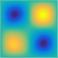
(a) Target state $u_{d}$

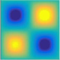
(b) State (coarse mesh)

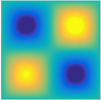
(c) State (fine mesh)

(d) Target control $z_{*}$

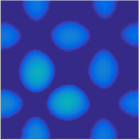
(e) Control (coarse mesh)

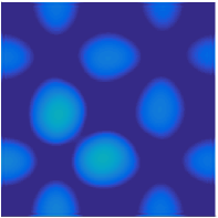
(f) Control (fine mesh)

Figure 2: Target and computed states (top), and controls (bottom) for (8.2c). Because the problem is ill-posed, the control is not exactly recovered, even though the state is well-matched.

Let $\Omega=(-1,1)^{2}$ represent the physical domain and $H^{1}(\Omega)$ denote the Sobolev space of functions in $L^{2}(\Omega)$, whose weak derivatives are also in $L^{2}(\Omega)$. Let $H_{0}^{1}(\Omega)\subset H^{1}(\Omega)$ be the Hilbert space of functions whose value on the boundary $\partial\Omega$ is zero. We solve the following 2D PDE-constrained control problem:

(8.2c) $$\mathop{\hbox{minimize}}_{u\in H_{0}^{1}(\Omega),\,z\in L^{2}(\Omega)} {\textstyle{\frac{1}{2}}}\int_{\Omega}\left(u-u_{d}\right)^{2}\mathrm{d}x+\tfrac{1}{2}\alpha\int_{\Omega}z^{2}\,\mathrm{d}x$$

$$\mathop{\hbox{subject to}} \begin{array}[t]{rll}-\nabla\cdot(z\nabla u)=&h&\mbox{in }\Omega,\\ u=&0&\mbox{on }\partial\Omega,\\ z\geq&0&\mbox{in }\Omega.\end{array}$$

Let $c=(0.2,0.2)$ and define $S_{1}=\{x\mid\|x-c\|_{2}\leq 0.3\}$ and $S_{2}=\{x\mid\|x-c\|_{1}\leq 0.6\}$. For a set $C$, define $I_{C}(x)=1$ if $x\in C$ and 0 otherwise. The target state $u_{d}$ is generated as the solution of the PDE with $z_{*}(x)=1+0.5\cdot I_{S_{1}}(x)+0.5\cdot I_{S_{2}}(x)$.

Table 1: Results from solving (8.2c) using KNITRO to solve (PP) with various $\eta$ in (8.2a) (left) and (8.2b) (right) to terminate the linear system solves. The top (resp. bottom) table records results for the smaller problem with $n=2050$, $m=1089$ (resp. larger problem with $n=20002$, $m=10201$). We record the number of function/gradient evaluations ($\#f,g$), Lagrangian Hessian (#$Hv$), Jacobian (#($Av$), and adjoint Jacobian (#$A^{T}\!v$) products.

$\eta$	Its.	#$f,g$	#$Hv$	#$Av$	#$A^{T}\!v$	Its.	#$f,g$	#$Hv$	#$Av$	#$A^{T}\!v$
$10^{-2\phantom{0}}$	46	64	2856	8436	8611	67	81	4374	12915	13145
$10^{-4\phantom{0}}$	43	55	2168	6642	6796	36	51	1458	4642	4781
$10^{-6\phantom{0}}$	35	46	2120	6876	7004	29	35	1194	4138	4238
$10^{-8\phantom{0}}$	39	50	2322	7833	7973	47	71	7062	22150	22340
$10^{-10}$	37	47	2236	8110	8242	43	58	3170	11565	11725
$10^{-2\phantom{0}}$	144	176	3662	12395	12892	100	126	3716	11702	12055
$10^{-4\phantom{0}}$	131	177	4002	14470	14956	83	117	2752	9264	9582
$10^{-6\phantom{0}}$	103	135	4386	15035	15409	88	132	4170	14421	14774
$10^{-8\phantom{0}}$	73	103	3250	11960	12244	101	133	3726	13878	14246
$10^{-10}$	79	109	4088	15527	15825	104	139	5378	20291	20674
	error-based termination					residual-based termination

The force term is $h(x_{1},x_{2})=-\sin(\omega x_{1})\sin(\omega x_{2})$, with $\omega=\pi-\tfrac{1}{8}$. The control variable $z$ represents the Poisson diffusion coefficients that we are trying to recover from the observed state $u_{d}$. We set $\alpha=10^{-4}$ as the regularization parameter. The problem is almost identical to that of Estrin et al. (2019a, §9.2) but with an additional bound constraint on the control variables (to ensure positivity of the diffusion coefficients).

We discretize (8.2c) in two ways using $P_{1}$ finite elements on a uniform mesh of $1089$ (resp. $10201$) triangular elements and employ an identical discretization for the optimization variables $z\in L^{2}(\Omega)$, obtaining a problem with $n_{z}=1089$ ($n_{z}=10201$) controls and $n_{u}=961$ ($n_{u}=9801$) states, so that $n=n_{u}+n_{z}$. The control variables are discretized using piecewise linear elements. There are $m=n_{u}$ constraints, as we must solve the PDE on every interior grid point. For each problem, the target state is discretized on a finer mesh with 4 times more grid points and then interpolated onto the meshes previously described.

Although the problem on the smaller mesh was solved without the bound constraint in (Estrin et al., 2019a, §9.2), the problem on the larger mesh could not be solved without explicitly enforcing the bound constraints because the control variables would go negative, causing the discretized PDE to be ill-defined.

We compute $x=(u,z)$ by applying KNITRO to (PP) with $\sigma=10^{-2}$, using $B_{2}(x)$ as the Hessian approximation (5.6b) and initial point $u_{0}=\mathbbm{1}$, $z_{0}=\mathbbm{1}$. We partition the Jacobian of the discretized constraints as $A(x)^{T}\!=\begin{bmatrix}A_{u}(x)^{T}\!&A_{z}(x)^{T}\!\end{bmatrix}$, where $A_{u}(x)\in\mathds{R}^{n\times n}$, $A_{z}(x)\in\mathds{R}^{m\times n}$ are the Jacobians for variables $u$, $z$ respectively. We use the preconditioner $\mathcal{P}(x)=A_{u}(x)^{T}\!A_{u}(x)$, which amounts to performing two solves of a variable-coefficient Poisson equation (performed via direct solves). For this preconditioner, because the only bound constraints are $z\geq 0$, $Q(x)=\mbox{blkdiag}(I,Z)$ with $Z=\operatorname{diag}(z)$, so that

$$\mathcal{P}^{-1}A(x)^{T}\!Q(x)A(x) =\mathcal{P}^{-1}(A_{u}(x)^{T}\!A_{u}(x)+A_{z}(x)ZA_{z}(x))$$

$$=I+\mathcal{P}^{-1}A_{z}(x)ZA_{z}(x).$$

Thus $\sigma_{\min}(A(x)\mathcal{P}^{-1/2})\geq 1$, allowing us to bound the error via LNLQ and to use both (8.2a) and (8.2b) as termination criteria.

We choose $\epsilon=10^{-8}$ in the stopping conditions (8.1). In Table 1 we vary $\eta$, which defines the termination criteria of the linear system solves (8.2), and we record the number of Hessian- and Jacobian-vector products. section 8.1 shows the target states and controls, and those that we recover on the two meshes (using (8.2a) and $\eta=10^{-10}$).

We observed that for the smaller problem, KNITRO converged in a moderate number of outer iterations in all cases. With (8.2a), we see that the number of Jacobian products tended to decrease as $\eta$ increased, except when $\eta=10^{-2}$ (for which the linear solves were too inaccurate). Using (8.2b) showed a less clear trend. In cases with comparable outer iteration numbers, larger $\eta$ resulted in fewer Jacobian products. However, for moderate $\eta$ the number of outer iterations proved to be significantly smaller, resulting in a more efficient solve than when $\eta$ was too small or too large.

For the larger problem with termination condition (8.2a), the number of outer iterations increased with $\eta$, the number of Lagrangian Hessian products fluctuated somewhat, and Jacobian products tended to decrease. The exception was $\eta=10^{-8}$, which hit the sweet spot of solving the linear systems sufficiently accurately to avoid many additional outer iterations, but without performing too many iterations for each linear solve. Using residual-based termination (8.2b) showed a less clear trend; Jacobian products roughly decreased with increasing $\eta$ while the Hessian products tended to oscillate. The sweet spot was hit with $\eta=10^{-4}$, where the fewest outer iterations and operator products were performed. For this problem, it appears that the dependence of performance on the accuracy of the linear solves as measured by the residual (8.2b) is much more nonlinear than when the linear solves are terminated according to the error (8.2a).

8.2 2D Poisson-Boltzmann problem

We now solve a control problem where the constraint is a 2D Poisson-Boltzmann equation:

(8.2r) $$\mathop{\hbox{minimize}}_{{u\in H_{0}^{1}(\Omega)},\ {z\in L^{2}(\Omega)}} {\textstyle{\frac{1}{2}}}\int_{\Omega}\left(u-u_{d}\right)^{2}\mathrm{d}x+\tfrac{1}{2}\alpha\int_{\Omega}z^{2}\,\mathrm{d}x$$

$$\mathop{\hbox{subject to}} \begin{array}[t]{rll}-\Delta u+\sinh(u)=&h+z&\mbox{in }\Omega,\\ u=&0&\mbox{on }\partial\Omega,\\ z\geq&0&\mbox{in }\Omega.\end{array}$$

We use the same notation and $\Omega$ as in section 8.1, with forcing term $h(x_{1},x_{2})=-\sin(\omega x_{1})\sin(\omega x_{2})$, $\omega=\pi-\tfrac{1}{8}$, and target state

$$u_{d}(x)=\begin{cases}10&\mbox{if }x\in[0.25,0.75]^{2}\\ 5&\mbox{otherwise.}\end{cases}$$

We discretized (8.2r) using $P_{1}$ finite elements on two uniform meshes with $1089$ (resp. $10201$) triangular elements, resulting in a problem with $n=2050$ ($n=20002$) variables and $m=961$ ($m=9801$) constraints. The initial point was $u_{0}=\mathbbm{1}$, $z_{0}=\mathbbm{1}$.

(a) Target state $u_{d}$

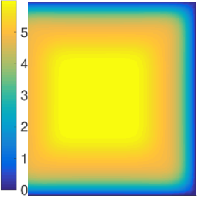
(b) State (coarse mesh)

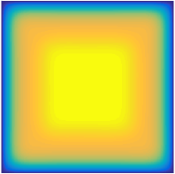
(c) State (fine mesh)

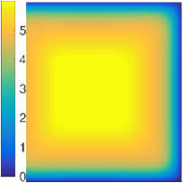
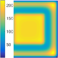
(d) Control (coarse mesh)

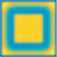
(e) Control (fine mesh)

Figure 3: Target and computed states (top), and controls (bottom) for (8.2r).

Table 2: Results from solving (8.2r) using KNITRO to optimize (PP) with various $\eta$ in (8.2a) (left) and (8.2b) (right) to terminate the linear system solves. The top (resp. bottom) table records results for the smaller problem with $n=2050$, $m=1089$ (resp. larger problem with $n=20002$, $m=10201$). We record the number of function/gradient evaluations ($\#f,g$), Lagrangian Hessian (#$Hv$), Jacobian (#($Av$), and adjoint Jacobian (#$A^{T}\!v$) products.

$\eta$	Its.	#$f,g$	#$Hv$	#$Av$	#$A^{T}\!v$	Its.	#$f,g$	#$Hv$	#$Av$	#$A^{T}\!v$
$10^{-2\phantom{0}}$	19	20	1242	3648	3708	19	20	1242	3669	3729
$10^{-4\phantom{0}}$	19	20	1252	3753	3813	19	20	1244	3762	3822
$10^{-6\phantom{0}}$	19	20	1236	3868	3928	19	20	1234	3916	3976
$10^{-8\phantom{0}}$	19	20	1244	4169	4229	19	20	1236	4286	4346
$10^{-10}$	19	20	1238	4725	4785	19	20	1250	4986	5046
$10^{-2\phantom{0}}$	30	37	1524	4426	4531	30	37	1524	4468	4573
$10^{-4\phantom{0}}$	30	37	1524	4574	4679	30	37	1524	4632	4737
$10^{-6\phantom{0}}$	30	37	1524	4813	4918	30	37	1558	5033	5138
$10^{-8\phantom{0}}$	30	37	1550	5396	5501	30	37	1550	5610	5715
$10^{-10}$	30	37	1550	6224	6329	30	37	1558	6582	6687
	error-based termination					residual-based termination

We performed the same experiment as in section 8.1 using $\sigma=10^{-1}$, and recorded the results in Table 2. The target and computed state, and computed controls on the two meshes using (8.2a) with $\eta=10^{-10}$ are given in section 8.2. We see that the results for both problems are more robust to changes in the accuracy of the linear solves. In all cases, the number of outer iterations and function/gradient evaluations were the same, and the number of Lagrangian Hessian products changed little. The number of Jacobian products steadily decreased with increasing $\eta$, with a 20–30% drop in Jacobian products from $\eta=10^{-10}$ to $\eta=10^{-2}$.

8.3 2D topology optimization

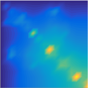
(a) State (small mesh)

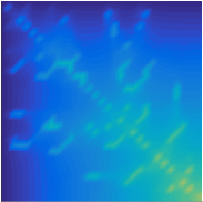
(b) State (med mesh)

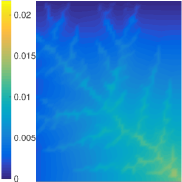
(c) State (big mesh)

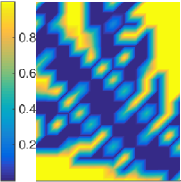
(d) Control (small mesh)

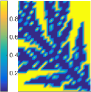
(e) Control (med mesh)

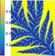
(f) Control (big mesh)

Figure 4: Target and computed states (top), and controls (bottom) for (8.2r).

We now solve the following 2D topology optimization problem from Gersborg-Hansen et al. (2006):

(8.2ag) $$\mathop{\hbox{minimize}}_{u\in H^{1}(\Omega),\,z\in L^{2}(\Omega)} \int_{\Omega}fu\,\mathrm{d}x$$

$$\mathop{\hbox{subject to}} \begin{array}[t]{rll}\displaystyle{\textstyle{\int_{\Omega}}z\,\mathrm{d}x}\leq&V&\\[2.0pt] -\nabla\cdot\left(k(z)\nabla u\right)=&f&\mbox{in }\Omega,\\ (k(z)\nabla u)\cdot\mathbf{n}=&0&\mbox{on }\partial\Omega_{1}=\{(x,y)\mid x=0\mbox{ or }y=1\},\\ u=&0&\mbox{on }\partial\Omega_{2}=\{(x,y)\mid x=1\mbox{ or }y=0\},\\ 0\leq z\leq&1&\mbox{in }\Omega,\end{array}$$

where $k(z):\Omega\rightarrow\Omega$ defined by $k(z)(x)=10^{-3}+(1-10^{-3})z(x)^{3}$ for $x\in\Omega$, and $\mathbf{n}$ is the outward unit normal vector. The domain is $\Omega=[0,1]^{2}$, with load vector $f=10^{-2}$, and $V=0.4$. We discretize (8.2ag) using finite elements as described by Gersborg-Hansen et al. (2006) on three grids: $16\times 16$, $32\times 32$, and $64\times 64$. This results in problems with $546$, $2114$, and $8321$ variables, and $256$, $1024$, and $4096$ equality constraints respectively. After discretization, we add a slack variable $s\geq 0$ for the first inequality constraint, so we have only equality constraints and bounds. The final problems then have one additional variable and constraint, with bounds on $z$ and $s$.

Table 3: Results from solving (8.2ag) using KNITRO to optimize (PP) with various $\eta$ in (8.2a) (left) and (8.2b) (right) to terminate the linear system solves. Each table corresponds to a different mesh, with $16\times 16$ (top, $n=546$, $m=257$), $32\times 32$ (middle, $n=2114$, $m=1025$), and $64\times 64$ (bottom, $n=8322$, $m=4097$). We record the number of function/gradient evaluations ($\#f,g$), Lagrangian Hessian (#$Hv$), Jacobian (#($Av$), and adjoint Jacobian (#$A^{T}\!v$) products. The symbol “*” indicates that the problem failed to converge to a feasible point after 500 iterations.

$\eta$	Its.	#$f,g$	#$Hv$	#$Av$	#$A^{T}\!v$	Its.	#$f,g$	#$Hv$	#$Av$	#$A^{T}\!v$
$10^{-2\phantom{0}}$	176	241	5296	15442	16342	147	230	3918	11462	12300
$10^{-4\phantom{0}}$	190	286	6052	17694	18743	171	238	5634	16774	17660
$10^{-6\phantom{0}}$	164	236	5266	15456	16329	143	199	3776	12019	12760
$10^{-8\phantom{0}}$	165	239	5350	15743	16626	176	251	7100	23222	24152
$10^{-10}$	185	261	9096	26934	27903	193	289	11420	39653	40714
$10^{-2\phantom{0}}$	219	311	6598	19745	20898	216	319	6272	18381	19555
$10^{-4\phantom{0}}$	196	265	5680	17073	18065	189	277	6382	18928	19949
$10^{-6\phantom{0}}$	190	271	6190	15638	16642	218	302	7960	24383	25508
$10^{-8\phantom{0}}$	184	272	4656	14050	15051	211	309	5868	19660	20799
$10^{-10}$	184	271	4396	13267	14265	203	291	5568	21526	22603
$10^{-2\phantom{0}}$	217	340	4340	13966	15204	*	*	*	*	*
$10^{-4\phantom{0}}$	226	348	4396	14068	15204	*	*	*	*	*
$10^{-6\phantom{0}}$	176	272	3232	11218	12211	191	291	3508	18326	19391
$10^{-8\phantom{0}}$	185	289	3356	11582	12635	196	296	3700	20888	21973
$10^{-10}$	204	298	4626	15412	16511	190	286	3480	23979	25028
	error-based termination					residual-based termination

We perform the same experiment as in section 8.1, using $\sigma=10^{-1}$ as the penalty parameter, and initial point $u_{0}={\textstyle{\frac{1}{2}}}V\mathbbm{1}$, $z_{0}={\textstyle{\frac{1}{2}}}V\mathbbm{1}$, $s_{0}=V-\sum z_{i}=0.2$. The linear constraint is kept explicit as in Section 6. The results are recorded in Table 3.

With (8.2a), the number of outer iterations tends to increase with the mesh size; the trend is less clear with (8.2b). It is well known that such topology optimization problems become increasingly difficult numerically (Sigmund and Petersson, 1998), and typically require the use of a filter prior to solving the nonlinear optimization problem to improve its conditioning. Meshes refined as far as $128\times 128$ could not be solved directly using (8.2ag).

For a given mesh, when using (8.2a) the trend is like before: as $\eta$ increases the number of Jacobian products decreases (and in this case, so do the numbers of outer iterations and Lagrangian Hessian products), but this is only true until $\eta$ becomes too large and the linear solves become too coarse, causing slowed convergence. When (8.2b) was used, we see a similar trend, except that when the linear solves are too coarse, KNITRO fails to converge.

8.4 Explicit linear constraints

We investigate the effect of maintaining the linear constraints explicitly (Section 6), using some problems from the CUTEst test set (Gould et al., 2003) that have linear constraints. We use KNITRO to minimize $\phi_{\sigma}$ with and without linear constraints, because it can handle them explicitly. We use the corrected semi-normal equations to perform linear solves, and Hessian approximation $B_{1}(x)$ (5.6a). The threshold penalty parameters (4.4) and (6.2) are computed from earlier optimal solutions when the linear constraints were kept implicit ($\sigma^{*}_{\mbox{{\footnotesize impl}}}$) and explicit ($\sigma^{*}_{\mbox{{\footnotesize expl}}}$) respectively. The results are recorded in Table 4.

We observe that maintaining the linear constraints explicitly decreases the penalty parameter for all problems except Channel400 ($\sigma^{*}=0$ in both cases). KNITRO fails to find an optimal solution when the linear constraints are implicit and $\sigma<\sigma^{*}_{\mbox{{\footnotesize impl}}}$. This is because in the equality-constrained case $\phi_{\sigma}$ is unbounded, and otherwise KNITRO stalls without converging to a feasible solution. When $\sigma$ is sufficiently large, both versions converge (with and without explicit constraints); in most cases keeping the constraints requires fewer iterations, except for Chain400. Although positive semidefiniteness of $\nabla^{2}\phi_{\sigma}(x^{*})$ is guaranteed in the relevant critical cone when $\sigma>\sigma^{*}$ (in either the implicit or explicit case), a larger value of $\sigma$ may sometimes be required because the curvature of $\phi_{\sigma}$ away from the solution may be larger or ill-behaved.

For the Channel problems, the threshold parameter is zero in both cases. However, KNITRO converges quickly when the linear constraints are kept explicit, but otherwise fails to converge in a reasonable number of iterations. This phenomenon for the Channel problems appears to be independent of $\sigma$ (more values were investigated than are reported here). Even if the penalty parameter does not decrease, it appears beneficial to maintain some of the constraints explicitly.

Table 4: Results for problems with linear constraints (first three rows have only equality constraints). $m_{\mbox{{\scriptsize lin}}}$ and $m_{\mbox{{\scriptsize nln}}}$ are the number of linear and nonlinear constraints; $\sigma^{*}_{\mbox{{\scriptsize impl}}}$ and $\sigma^{*}_{\mbox{{\scriptsize expl}}}$ are threshold penalty parameters when the linear constraints are handled implicitly and explicitly; $\sigma$ is the penalty parameter. The last two columns give the number of iterations before convergence; the symbol “$*$” indicates that unboundedness was detected, and “-” that 100 iterations were performed without converging. The solver exits when unboundedness is detected or an iterate satisfies (8.1) with $\epsilon=10^{-8}$.

Problem	$n$	$m_{\mbox{{\scriptsize lin}}}$	$m_{\mbox{{\scriptsize nln}}}$	$\sigma^{*}_{\mbox{{\scriptsize impl}}}$	$\sigma^{*}_{\mbox{{\scriptsize expl}}}$	$\sigma$	Impl.	Expl.
Chain400	802	402	1	0.0012	0	$10^{-3}$	$*$	10
						0.002	7	10
Channel400	1600	800	800	0	0	$10^{-3}$	$-$	5
						$1$	$-$	5
hs113	18	3	5	6.61	3.39	6	$*$	42
						$7$	28	17
prodpl0	69	25	4	211.9	13.7	$40$	$-$	43
						$300$	$-$	30
prodpl1	69	25	4	60.8	3.56	$10$	$-$	22
						$70$	89	41
synthes3	38	23	19	6.00	0.66	$2$	$-$	12
						$7$	$35$	18

9 Discussion and concluding remarks

We derived a smooth extension of the penalty function by Fletcher (1970) as an extension to the implementation of Estrin et al. (2019a) to include bound constraints. Our implementation is particularly promising for problems where augmented linear systems (5.8) can be solved efficiently. We further demonstrated the merits of the approach on several PDE-constrained optimization problems.

Some limitations that are shared with the equality-constrained case are avenues for future work. These include dealing with the highly nonlinear nature of the penalty function, developing robust penalty parameter updates and linear solve tolerance rules (for inexact optimization solvers), preconditioning the trust-region subproblems, and using cheaper second-derivative approximations (e.g., quasi-Newton updates) in conjunction with Hessian approximations (5.6a)–(5.6b). Possible approaches for dealing with these issues are discussed by Estrin et al. (2019a, §10).

Bound constraints provide additional challenges for future work on top of the equality-constrained case. For example, we would like to extend the theory to problems with weaker constraint qualifications than (A2)–(A3). A regularization approach as in (Estrin et al., 2019a, §6) can be employed when bound constraints are present, but it may need to be refined to obtain similar convergence guarantees when (A2) applies only at KKT points.

Another challenge is the possible numerical instability when iterates are close to the bounds, if the quantity $A(x)^{T}\!Q(x)A(x)$ becomes ill-conditioned. It would help to develop a specialized bound-constrained interior-point Newton-CG trust-region solver for (PP) that carefully controls the distance to the bounds and attempts to minimize the number of approximate penalty Hessian products (as Hessian products are the most computationally intensive operation requiring two linear solves). We can also investigate other functions $Q(x)$ to approximate the complementarity conditions for KKT points, as different forms may have different advantages and limitations; for example, (2.5) may cause premature termination if $x^{*}$ is far from its bounds.

Our Matlab implementation can be found at https://github.com/optimizers/FletcherPenalty. To highlight the flexibility of Fletcher’s approach, we implemented several options for applying various solvers to the penalty function and for solving the augmented systems, and other options discussed along the way.

Appendix A Maintaining explicit constraints

We discuss technical details about the penalty function when some of the constraints are linear and maintained explicitly as in (6.1). We define $W_{\sigma}(x)=\nabla w_{\sigma}(x)\in\mathds{R}^{n\times m_{2}}$, and $C(x)=\begin{bmatrix}A(x)&B\end{bmatrix}$ as the Jacobian of all constraints. The operators $g_{\sigma}(x)$, $H_{\sigma}(x)$, $S(x,v)$ and $T(x,w)$ are still defined over all constraints (e.g., $g_{\sigma}(x):=g(x)-A(x)y_{\sigma}(x)-Bw_{\sigma}(x)$), not just the nonlinear ones, and so they act on $C(x)$ and not just $A(x)$. Define

(8.2a) $$g_{\sigma}^{y}(x)=g(x)-A(x)y_{\sigma}(x)$$

as the gradient of the partial Lagrangian with respect to the nonlinear constraints $c(x)$ only (note that the linear constraints do not affect $H_{\sigma}$). The gradient and Hessian of the penalty function become

(8.2ba) $$\nabla\phi_{\sigma}(x) =g_{\sigma}^{y}(x)-Y_{\sigma}(x)c(x),$$

(8.2bb) $$\nabla^{2}\phi_{\sigma}(x) =H_{\sigma}(x)-A(x)Y_{\sigma}(x)^{T}-Y_{\sigma}(x)A(x)^{T}-\nabla_{x}\left[Y_{\sigma}(x)c\right].$$

We restate the optimality conditions for (NP-EXP) in terms of the penalty function. To do so, define the critical cones for (NP-EXP) and (6.1), respectively, as

$$\macc@depth\char 1\relax\frozen@everymath{\macc@group}\macc@set@skewchar\macc@nested@a 111{}_{\phi}(x^{*},z^{*})=\mathcal{C}_{\phi}(x^{*},z^{*})\cap\{p\mid B^{T}\!p=0\},\qquad\macc@depth\char 1\relax\frozen@everymath{\macc@group}\macc@set@skewchar\macc@nested@a 111{}(x^{*},z^{*})=\mathcal{C}(x^{*},z^{*})\cap\{p\mid B^{T}\!p=0\}.$$

Definition A.1 (First-order KKT point).

A point $(x^{*},z^{*})$ is a first-order KKT point of (NP-EXP) if for any $\sigma\geq 0$ the following hold:

(8.2ca) $$\ell\leq x^{*} \leq u,$$

(8.2cb) $$c(x^{*}) =0,$$

(8.2cc) $$B^{T}\!x^{*} =d,$$

(8.2cd) $$\nabla\phi_{\sigma}(x^{*}) =Bw^{*}+z^{*},$$

(8.2ce) $$z^{*}_{j} =0\qquad\mbox{if }j\notin\mathcal{A}(x^{*}),$$

(8.2cf) $$z^{*}_{j} \geq 0\qquad\mbox{if }x^{*}_{j}=\ell_{j},$$

(8.2cg) $$z^{*}_{j} \leq 0\qquad\mbox{if }x^{*}_{j}=u_{j}.$$

Then $y^{*}:=y_{\sigma}(x^{*})$ and $w^{*}:=w_{\sigma}(x^{*})$ comprise the Lagrange multipliers of (NP-EXP) associated with $x^{*}$. Note that by (A3), inequalities (8.2cf) and (8.2cg) are strict.

Definition A.2 (Second-order KKT point).

The first-order KKT point $(x^{*},z^{*})$ satisfies the second-order necessary KKT condition for (NP-EXP) if for any $\sigma\geq 0$,

(8.2d) $$p^{T}\nabla^{2}\phi_{\sigma}(x^{*})p\geq 0\quad\hbox{for all $p\in\macc@depth\char 1\relax\frozen@everymath{\macc@group}\macc@set@skewchar\macc@nested@a 111{}(x^{*},z^{*})$. }$$

The condition is sufficient if the inequality is strict.

Remark A.3.

As before, if (8.2cb) is omitted, Definition A.1 defines first-order KKT points of (6.1). Similarly, replacing $\macc@depth\char 1\relax\frozen@everymath{\macc@group}\macc@set@skewchar\macc@nested@a 111{}(x^{*},z^{*})$ by $\macc@depth\char 1\relax\frozen@everymath{\macc@group}\macc@set@skewchar\macc@nested@a 111{}_{\phi}(x^{*},z^{*})$ in Definition A.2 defines second-order KKT points of (6.1).

A.1 Proof of Theorem 6.1

Observe that the multiplier estimates $y_{\sigma}(x)$ and $w_{\sigma}(x)$ satisfy

(8.2e) $$C(x)^{T}Q(x)C(x)\begin{bmatrix}y_{\sigma}(x)\\ w_{\sigma}(x)\end{bmatrix}=C(x)^{T}Q(x)g(x)-\sigma\begin{bmatrix}c(x)\\ B^{T}\!x-d\end{bmatrix}.$$

Proof of (6.4a): We drop the argument $x$ from operators and assume that all are evaluated at $\bar{x}$. Because $\bar{x}$ is a first-order KKT point for (6.1), we need only show that $c(\bar{x})=0$. Further, $Q(\nabla\phi_{\sigma}-Bw^{*})=0$ at $\bar{x}$, or equivalently,

$$QBw^{*}=Q\left(g-Ay_{\sigma}-Y_{\sigma}c\right).$$

Multiplying both sides by $C^{T}\!$ and using (8.2e) we have

$$\begin{bmatrix}A^{T}\!QBw^{*}\\ B^{T}\!QBw^{*}\end{bmatrix}=\sigma\begin{bmatrix}c\\ 0\end{bmatrix}+\begin{bmatrix}A^{T}\!QBw_{\sigma}\\ B^{T}\!QBw_{\sigma}\end{bmatrix}-\begin{bmatrix}A^{T}\!QY_{\sigma}c\\ B^{T}\!QY_{\sigma}c\end{bmatrix},$$

so that $w_{\sigma}=w^{*}+(B^{T}\!QB)^{-1}B^{T}\!QY_{\sigma}c$. Substituting $w_{\sigma}(\bar{x})$ into the first block of equations and rearranging gives

$$AQ^{1/2}{\bar{P\mkern 5.0mu}\mkern-5.0mu}{}_{Q^{1/2}B}Q^{1/2}Y_{\sigma}c=\sigma c.$$

The triangle inequality gives $\sigma\|c\|\leq\|A^{T}Q^{1/2}{\bar{P\mkern 5.0mu}\mkern-5.0mu}{}_{Q^{1/2}B}Q^{1/2}Y_{\sigma}\|\|c\|$, implying $c=0$. Then $w_{\sigma}=w^{*}$ and $\bar{x}$ is a first-order KKT point for (NP-EXP).

Proof of (6.4b): As in the proof of (4.7b), we differentiate (8.2e) to obtain

(8.2f) $$C(x)^{T}\!Q(x)C(x)\begin{bmatrix}Y_{\sigma}(x)^{T}\\ W_{\sigma}(x)^{T}\end{bmatrix}$$

$$\qquad=C(x)^{T}\!\left[Q(x)H_{\sigma}(x)-\sigma I+R(x,g_{\sigma}(x))\right]+S(x,Q(x)g_{\sigma}(x)).$$

For the remainder of the proof, we assume all operators are evaluated at $x^{*}$. Because $x^{*}$ satisfies first-order conditions (8.2c), $Qg_{\sigma}=0$ independently of $\sigma$, so $S(Qg_{\sigma})=0$. Let $P_{Q^{1/2}C}:=P_{Q^{1/2}C(x^{*})}(x^{*})$, so that from (8.2f) we have

(8.2g) $$Q^{1/2}\left(AY_{\sigma}^{T}+BW_{\sigma}^{T}\right)Q^{1/2}=P_{Q^{1/2}C}\left[Q^{1/2}H_{\sigma}Q^{1/2}-\sigma I+R(g_{\sigma})Q^{1/2}\right].$$

Observe that if $p\in\macc@depth\char 1\relax\frozen@everymath{\macc@group}\macc@set@skewchar\macc@nested@a 111{}_{\phi}(x^{*},z^{*})$, then $p=Q^{1/2}{\bar{p\mkern 2.0mu}\mkern-2.0mu}{}$ for some ${\bar{p\mkern 2.0mu}\mkern-2.0mu}{}\in\macc@depth\char 1\relax\frozen@everymath{\macc@group}\macc@set@skewchar\macc@nested@a 111{}_{\phi}(x^{*},z^{*})$. Because $Q^{1/2}g_{\sigma}=0$, we have $R(g_{\sigma})p=0$.

Substituting (8.2g) into (8.2bb), and $P_{Q^{1/2}C}+{\bar{P\mkern 5.0mu}\mkern-5.0mu}{}_{Q^{1/2}C}=I$ gives

$$p^{T}\nabla^{2}\phi_{\sigma}(x^{*})p\geq 0$$

$$\iff {\bar{p\mkern 2.0mu}\mkern-2.0mu}{}^{T}Q^{1/2}\left(H_{\sigma}-AY_{\sigma}^{T}\!-Y_{\sigma}A^{T}\right)Q^{1/2}{\bar{p\mkern 2.0mu}\mkern-2.0mu}{}\geq 0$$

$$\iff {\bar{p\mkern 2.0mu}\mkern-2.0mu}{}^{T}\left({\bar{P\mkern 5.0mu}\mkern-5.0mu}{}_{Q^{1/2}C}Q^{1/2}H_{\sigma}Q^{1/2}{\bar{P\mkern 5.0mu}\mkern-5.0mu}{}_{Q^{1/2}C}-P_{Q^{1/2}C}Q^{1/2}H_{\sigma}Q^{1/2}P_{Q^{1/2}C}+2\sigma P_{Q^{1/2}C}\right){\bar{p\mkern 2.0mu}\mkern-2.0mu}{}$$

$$\qquad-p^{T}\!\left(BW_{\sigma}^{T}\!+W_{\sigma}B^{T}\!\right)p\geq 0.$$

Because $H_{\sigma}(x^{*})=H_{\scriptscriptstyle L}(x^{*},y^{*})$, $0=B^{T}p=B^{T}Q^{1/2}{\bar{p\mkern 2.0mu}\mkern-2.0mu}{}$, we can write ${\bar{p\mkern 2.0mu}\mkern-2.0mu}{}={\bar{P\mkern 5.0mu}\mkern-5.0mu}{}_{\bar{B}}q$ with $\bar{B}=Q^{1/2}B$ and hence

$$0\leq p^{T}\nabla^{2}\phi_{\sigma}(x^{*}_{2})p$$

$$\iff 0\preceq {\bar{P\mkern 5.0mu}\mkern-5.0mu}{}_{\bar{B}}{\bar{P\mkern 5.0mu}\mkern-5.0mu}{}_{Q^{1/2}C}H_{\scriptscriptstyle L}(x^{*},y^{*}){\bar{P\mkern 5.0mu}\mkern-5.0mu}{}_{Q^{1/2}C}{\bar{P\mkern 5.0mu}\mkern-5.0mu}{}_{\bar{B}}$$

$$\qquad-{\bar{P\mkern 5.0mu}\mkern-5.0mu}{}_{\bar{B}}P_{Q^{1/2}C}H_{\scriptscriptstyle L}(x^{*},y^{*})P_{Q^{1/2}C}{\bar{P\mkern 5.0mu}\mkern-5.0mu}{}_{\bar{B}}+2\sigma{\bar{P\mkern 5.0mu}\mkern-5.0mu}{}_{\bar{B}}P_{Q^{1/2}C}{\bar{P\mkern 5.0mu}\mkern-5.0mu}{}_{\bar{B}}.$$

As before, the first term is positive semi-definite, so we only need that

$$-{\bar{P\mkern 5.0mu}\mkern-5.0mu}{}_{\bar{B}}P_{Q^{1/2}C}H_{\scriptscriptstyle L}(x^{*},y^{*})P_{Q^{1/2}C}{\bar{P\mkern 5.0mu}\mkern-5.0mu}{}_{\bar{B}}+2\sigma{\bar{P\mkern 5.0mu}\mkern-5.0mu}{}_{\bar{B}}P_{Q^{1/2}C}{\bar{P\mkern 5.0mu}\mkern-5.0mu}{}_{\bar{B}}\succeq 0,$$

which is equivalent to $\sigma\geq\bar{\sigma}$.

A.1.1 Evaluating the penalty function and derivatives

We again drop the arguments on functions and assume they are evaluated at a point $x$ for some $\sigma$:

$$y=y_{\sigma}(x),\quad A=A(x),\quad Y_{\sigma}=Y_{\sigma}(x),\quad H_{\sigma}=H_{\sigma}(x),\quad S_{\sigma}=S_{\sigma}(x,g_{\sigma}(x)),\quad\hbox{etc.}$$

We focus on the nonsymmetric linear systems; the corresponding symmetric linear systems can be derived similarly to Section 5.

The multipliers for evaluating the penalty function are obtained by solving

(8.2h) $$\begin{bmatrix}I&A&B\\ A^{T}\!Q&&\\ B^{T}\!Q&&\end{bmatrix}\begin{bmatrix}g_{\sigma}\\ y_{\sigma}\\ w_{\sigma}\end{bmatrix}=\begin{bmatrix}g\\ \sigma c\\ \sigma(Bx-d)\end{bmatrix}.$$

To compute the gradient and Hessian products, we use the identity

(8.2i) $$C^{T}\!QC\begin{bmatrix}Y_{\sigma}^{T}\\ W_{\sigma}^{T}\end{bmatrix}=C^{T}\!\left[QH_{\sigma}-\sigma I+R_{\sigma}\right]+S_{\sigma}$$

to obtain the necessary products with $Y_{\sigma}$ and $Y_{\sigma}^{T}\!$. Observe that

$$Y_{\sigma}u=\begin{bmatrix}Y_{\sigma}&W_{\sigma}\end{bmatrix}\begin{bmatrix}u\\ 0\end{bmatrix},\qquad Y_{\sigma}^{T}\!v=\begin{bmatrix}I&0\end{bmatrix}\begin{bmatrix}Y_{\sigma}^{T}\\ W_{\sigma}^{T}\end{bmatrix}v,$$

so that Algorithm 1 and Algorithm 2 can be applied.

Note that to compute the gradient in (8.2ba), $g_{\sigma}^{y}$ is not available directly from the solution to (8.2h) and must be computed explicitly using (8.2a).

Approximate products with $\nabla^{2}\phi_{\sigma}$ can be computed via

$$\nabla^{2}\phi_{\sigma} \approx B_{1}:=H_{\sigma}-AY_{\sigma}^{T}-Y_{\sigma}A^{T}$$

$$\phantom{\approx B_{1}:}=H_{\sigma}-\begin{bmatrix}A&0\end{bmatrix}(C^{T}\!QC)^{-1}C^{T}\!(QH_{\sigma}-\sigma I+R_{\sigma})-\begin{bmatrix}A&0\end{bmatrix}(C^{T}\!QC)^{-1}S_{\sigma}$$

$$\phantom{\approx B_{1}:=}\qquad-(H_{\sigma}Q-\sigma I+R_{\sigma})C(C^{T}\!QC)^{-1}\begin{bmatrix}A^{T}\\ 0\end{bmatrix}-S_{\sigma}(C^{T}\!QC)^{-1}\begin{bmatrix}A^{T}\\ 0\end{bmatrix}$$

$$\approx B_{2}:=H_{\sigma}-\begin{bmatrix}A&0\end{bmatrix}(C^{T}\!QC)^{-1}C^{T}\!(QH_{\sigma}-\sigma I+R_{\sigma})$$

$$\phantom{\approx B_{1}:=}\qquad-(H_{\sigma}Q-\sigma I+R_{\sigma})C(C^{T}\!QC)^{-1}\begin{bmatrix}A^{T}\\ 0\end{bmatrix}.$$

For products with the weighted-pseudoinverse and its transpose, we can compute

$$\begin{bmatrix}u_{1}\\ u_{2}\end{bmatrix}=(C^{T}\!QC)^{-1}C^{T}\!v,\qquad v=C(C^{T}\!QC)^{-1}\begin{bmatrix}u_{1}\\ u_{2}\end{bmatrix}$$

by solving the respective block systems

(8.2j) $$\begin{bmatrix}I&QA&QB\\ A^{T}\!&&\\ B^{T}\!&&\end{bmatrix}\begin{bmatrix}t\\ u_{1}\\ u_{2}\end{bmatrix}=\begin{bmatrix}v\\ 0\\ 0\end{bmatrix},\qquad\begin{bmatrix}I&A&B\\ A^{T}\!Q&&\\ B^{T}\!Q&&\end{bmatrix}\begin{bmatrix}v\\ t_{1}\\ t_{2}\end{bmatrix}=\begin{bmatrix}0\\ -u_{1}\\ -u_{2}\end{bmatrix}.$$

Thus we can obtain the same types of Hessian approximations as (5.6), again with two augmented system solves per product.

References

Anitescu (2000)
M. Anitescu.
On solving mathematical programs with complementarity constraints as
nonlinear programs.
Preprint ANL/MCS-P864-1200, Argonne National Laboratory, 2000.
Arioli (2013)
M. Arioli.
Generalized Golub-Kahan bidiagonalization and stopping criteria.
SIAM J. Matrix Anal. Appl., 34(2):571–592, 2013.
10.1137/120866543.
Bertsekas (1975)
D. P. Bertsekas.
Necessary and sufficient conditions for a penalty method to be exact.
Math. Program., 9:87–99, 1975.
Bertsekas (1982)
D. P. Bertsekas.
Constrained Optimization and Lagrange Multiplier Methods.
Academic Press, New York, 1982.
Björck and Paige (1994)
A. Björck and C. C. Paige.
Solution of augmented linear systems using orthogonal factorizations.
BIT, 34(1):1–24, 1994.
10.1007/BF01935013.
Boggs et al. (1992)
P. T. Boggs, J. W. Tolle, and A. J. Kearsley.
A merit function for inequality constrained nonlinear programming
problems.
Internal Report NISTIR 4702, Applied and Computational
Mathematics Division, National Institute of Standards and
Technology, Gaithersburg, MD, USA, 1992.
Byrd et al. (2006)
R. H. Byrd, J. Nocedal, and R. A. Waltz.
KNITRO: An integrated package for nonlinear optimization.
In G. di Pillo and M. Roma, editors, Large-Scale Nonlinear
Optimization, pages 35–59. Springer-Verlag, New York, 2006.
Chen (2000)
X. Chen.
Smoothing methods for complementarity problems and their
applications: a survey.
J. Oper. Res. Soc. Japan, 43(1):32–47,
2000.
ISSN 0453-4514.
10.1016/S0453-4514(00)88750-5.
New trends in mathematical programming (Kyoto, 1998).
Conn et al. (2000)
A. R. Conn, N. I. M. Gould, and Ph. L. Toint.
Trust-Region Methods.
MPS-SIAM Series on Optimization. SIAM, Philadelphia, 2000.
Craig (1955)
J. E. Craig.
The N-step iteration procedures.
Journal of Mathematics and Physics, 34(1):64–73, 1955.
Di Pillo and Grippo (1984)
G. Di Pillo and L. Grippo.
A class of continuously differentiable exact penalty function
algorithms for nonlinear programming problems.
In E. P. Toft-Christensen, editor, System Modelling and
Optimization, page 246–256. Springer-Verlag, Berlin, 1984.
Di Pillo and Grippo (1985)
G. Di Pillo and L. Grippo.
A continuously differentiable exact penalty function for nonlinear
programming problems with inequality constraints.
SIAM J. Control Optim., 23(1):72–84,
1985.
ISSN 0363-0129.
10.1137/0323007.
Estrin and Greif (2018)
R. Estrin and C. Greif.
SPMR: a family of saddle-point minimum residual solvers.
SIAM J. Sci. Comput., 40(3):A1884–A1914,
2018.
ISSN 1064-8275.