Constraining the Milky Way Mass Profile with Phase-Space Distribution of Satellite Galaxies

Abstract

We estimate the Milky Way (MW) halo properties using satellite kinematic data including the latest measurements from Gaia DR2. With a simulation-based 6D phase-space distribution function (DF) of satellite kinematics, we can infer halo properties efficiently and without bias, and handle the selection function and measurement errors rigorously in the Bayesian framework. Applying our DF from the EAGLE simulation to 28 satellites, we obtain an MW halo mass of $M=1.23_{-0.18}^{+0.21}\times 10^{12}M_{\odot}$ and a concentration of $c=9.4_{-2.1}^{+2.8}$ with the prior based on the $M$-$c$ relation. The inferred mass profile is consistent with previous measurements but with better precision and reliability due to the improved methodology and data. Potential improvement is illustrated by combining satellite data and stellar rotation curves. Using our EAGLE DF and best-fit MW potential, we provide much more precise estimates of kinematics for those satellites with uncertain measurements. Compared to the EAGLE DF, which matches the observed satellite kinematics very well, the DF from the semi-analytical model based on the dark-matter-only simulation Millennium II (SAM-MII) over-represents satellites with small radii and velocities. We attribute this difference to less disruption of satellites with small pericenter distances in the SAM-MII simulation. By varying the disruption rate of such satellites in this simulation, we estimate a $\sim 5\%$ scatter in the inferred MW halo mass among hydrodynamics-based simulations.

1 Introduction

The total mass and density distribution for the Milky Way (MW) dark matter halo are of great importance to various astrophysical studies. Most of the methods that have been proposed to constrain the MW mass profile make use of dynamical tracers (see Wang et al. 2019 for review). The mass distribution of the inner halo (within $\sim 40\,\mathrm{kpc}$) has been relatively well constrained by the kinematics of masers, stars, stellar streams, and globular clusters. However, the profile of the outer halo and the virial mass show less agreement (see Eadie & Jurić 2019; Wang et al. 2019 for comparisons of recent estimates, and McMillan 2011 for critical comments). Due to the limited number of tracers and lack of good data, different model assumptions (including profile extrapolation) and their associated systematics lead to a factor of $\gtrsim 2$ disagreement in the halo mass estimate.

Satellite galaxies are the preferred tracers for the outer halo in several aspects. First of all, thanks to their relatively high luminosities and extended spatial distribution, currently they are the only tracers with sufficient statistics for the very outer halo ($\gtrsim 100$ kpc). Further, their kinematics is well understood in the framework of hierarchical structure formation and accurately modeled by modern cosmological simulations, which makes their dynamical modeling more reliable. In addition, satellite galaxies closely trace the underlying phase-space distribution of dark matter particles, while halo stars are less phase-mixed (Han et al., 2019).

A popular method for dynamical modeling of outer halo tracers is based on the phase-space distribution function (DF). As the complete statistical description of a stationary dynamical system, the DF can maximize the use of kinematic data. The DF method has been widely used for tracers like stars, globular clusters, and satellite galaxies (e.g., Little & Tremaine 1987; Kochanek 1996; Wilkinson & Evans 1999; Sakamoto et al. 2003; Deason et al. 2012; Williams & Evans 2015a; Binney & Wong 2017; Eadie & Jurić 2019; Posti & Helmi 2019; Vasiliev 2019). However, despite many analytical and simulation-based attempts (e.g., Cuddeford 1991; Evans & An 2006; Wojtak et al. 2008; Posti et al. 2015; Williams & Evans 2015b) since the seminal work of Lynden-Bell (1967), an accurate and explicit form of the DF for tracers of halos remains to be found and verified. As shown by Wang et al. (2015) and Han et al. (2016a), unjustified assumptions (e.g., constant velocity anisotropy) in constructing the DF may lead to substantially biased results. Fortunately, we can construct the DF for satellite galaxies directly from cosmological simulations.

Li et al. (2017) constructed the probability density function (PDF) $p(E,L)$ of the satellite orbital energy $E$ and angular momentum $L$ directly from cosmological simulations. They found that the internal dynamics of different halos are very similar when normalized by the corresponding virial scales. Using this feature and the constructed $p(E,L)$, they developed a method to estimate the halo mass from satellite kinematics. Callingham et al. (2019) made some improvement of this method. With the kinematic data of 10 luminous satellites, they found an MW halo mass of $1.17^{+0.21}_{-0.15}\times 10^{12}M_{\odot}$. However, the PDF $p(E,L)$ in the 2D orbital space of $E$ and $L$ differs from the DF $f({\bm{r}},{\bm{v}})$ in the 6D phase space of position $\bm{r}$ and velocity $\bm{v}$. Because the orbital energy $E$ is not directly observable, the use of $p(E,L)$ to estimate the halo mass requires calibration with mock samples. In contrast, as shown in Li et al. (2019), the use of the DF $f({\bm{r}},{\bm{v}})$, which describes the direct observables ${\bm{r}}$ and ${\bm{v}}$, automatically gives unbiased and precise estimates of halo properties. The precision of this DF method can be attributed to the incorporation of both the orbital distribution described by $p(E,L)$ and the radial distribution along each orbit that was the basis of the orbital PDF method (Han et al., 2016b).

Assuming steady state for satellites in the host halo potential, Li et al. (2019) used both the similarity of the internal dynamics for different halos and the universal Navarro–Frenk–White (NFW, Navarro et al. 1996) density profile in constructing the DF from a cosmological simulation. Consequently, they were able to estimate both the halo mass $M$ and the concentration $c$ for the NFW profile, thereby obtaining the mass distribution. Tests with mock samples showed that this method is valid and accurate, as well as more precise than pure steady-state methods, including the Jeans equation and Schwarzschild modeling. The halo-to-halo scatter due to diversities in halo formation history and environment results in an intrinsic uncertainty of only $\sim 10\%$ for the halo mass. In addition, this method facilitates a rigorous and straightforward treatment of various observational effects, including selection functions and observational errors. This feature is especially important for outer halo tracers, for which these effects are much more severe and their improper treatment can lead to serious bias.

In this paper, we apply the DF method of Li et al. (2019) to estimate the MW halo properties using kinematic data on 28 satellites, including precise proper motion measurements by Gaia DR2 (Gaia Collaboration et al., 2018a). This sample is optimized for the outer halo. The improved methodology and observational data enable us to obtain the currently best estimates of the MW halo mass and outer halo profile. Our results weakly depend on the simulation used to construct the DF. We quantify this model dependence by comparing the results from the hydrodynamics-based EAGLE simulation and the semi-analytical model based on the dark-matter-only simulation Millennium II. We confirm by the goodness-of-fit that the EAGLE simulation provides a better description of the kinematics of MW satellites.

The plan of this paper is as follows. We describe the satellite sample and the corresponding selection function in Section 2. We outline our method in Section 3 and present the results in Section 4. We make comparisons with previous works and show how our results can be improved by combining different tracer populations in Section 5. We summarize our results and give conclusions in Section 6.

In this paper, the halo mass $M$ and concentration $c$ refer to the total mass including the baryonic contribution. We define $M$ as the mass enclosed by the virial radius $R$, within which the average density is 200 times the critical density of the present universe, $\rho_{\rm cri}={3H_{0}^{2}}/({8\pi G})$. Here, $H_{0}=67.77\,\mathrm{km\,s^{-1}Mpc^{-1}}$ is the Hubble constant and $G$ is the gravitational constant.

2 Observation data

In this work, we use the recent MW satellite data, including the coordinates, luminosities, distances, line-of-sight velocities, and proper motions, compiled by Riley et al. (2019). When available, we adopt the “gold” proper motions in Riley et al. (2019), which usually represent more precise measurements due to the larger sample of member stars used. Furthermore, this compilation omitted satellites that have been disrupted or whose nature is still under debate.

2.1 Satellite sample

We select our sample of satellites based on their distance to the Galactic center (GC), $r$. Considering $r=262\pm 9\,\mathrm{kpc}$ for Leo I, the farthest satellite with measured proper motion in Riley et al. (2019), we only use those satellites with $r<280$ kpc. Varying this upper limit within 100–300 $\mathrm{kpc}$ does not change our results (see Section 4.2). We also exclude satellites with $r<40\,\mathrm{kpc}$ to avoid complications from the MW disk. Based on the above criteria ($40<r<280\,\mathrm{kpc}$), we have selected 28 satellites, whose properties are listed in Table 2 of Appendix A. The median distance to the sun for this sample is $\sim 100$ kpc.

As our model uses kinematic data relative to the GC but the satellite data are given in the Heliocentric Standard of Rest (HSR) frame, we transform the HSR data (coordinates, distance, line-of-sight velocity, and proper motion) to quantities in the Galactocentric Standard of Rest (GSR) frame with the Python package Astropy (2013). We adopt the following position and velocity of the Sun in the GSR frame (Bland-Hawthorn & Gerhard, 2016): a radial distance of $8.2\,\mathrm{kpc}$ in the Galactic plane, a vertical distance of $25\,\mathrm{pc}$ above this plane, and $(U_{\odot},V_{\odot},W_{\odot})=(10,248,7)\,\mathrm{km\,s}^{-1}$, where $U_{\odot}$ is the velocity toward the GC, $V_{\odot}$ is positive in the direction of Galactic rotation, and $W_{\odot}$ is positive toward the north Galactic pole. Measurement errors in the distance, line-of-sight velocity, and proper motion are taken into account as follows. Assuming that the error in each observable is Gaussian and mutually independent, we generate 2000 Monte Carlo realizations of the HSR data for each satellite according to these errors and transform each realization to propagate the errors to the GSR data. The GSR data thus obtained will be used as the direct input for our model.

2.2 Selection function

Satellite samples discovered by sky surveys inevitably suffer from incompleteness [see e.g., Koposov et al. 2008; Walsh et al. 2009 for Sloan Digital Sky Survey (SDSS) and Jethwa et al. 2016 for Dark Energy Survey (DES)]. Here, we only use a subset of MW satellites with complete astrometric data measured by Gaia DR2, which represents a uniform survey with a well-understood selection function. Below we derive a good approximation of this selection function.

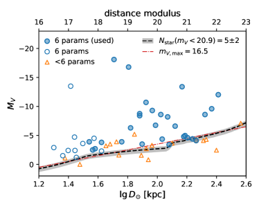
Figure 1: Heliocentric distance $D_{\odot}$ and absolute magnitude $M_{V}$ for known MW satellites. Satellites with complete kinematic data (Riley et al., 2019) measured by Gaia are shown as circles (labeled “6 params” for 6 parameters), and the rest (taken from Simon 2019) are shown as triangles. The 28 satellites with $40<r<280\,\mathrm{kpc}$ used in this work are marked by filled blue circles. The black dashed curve shows the completeness distance $R_{\mathrm{obs,max}}$ for Gaia proper motion measurement at each $M_{V}$, which distinguishes the circles and triangles very well. The red dash-dotted line indicates an apparent magnitude of $m_{V\!,\max}=16.5$ for reference. See text for details.

Gaia DR2 can usually measure the proper motion of a satellite reliably only when it contains at least $\sim 5$ member stars brighter than the observation limit (apparent $G$-band magnitude of $m_{G}\!\sim\!20.9$ forDR2). The detection rate drops sharply below this threshold (see black dashed curve in Figure 1). Therefore, we can estimate the completeness radius $R_{\mathrm{obs,max}}$ as a function of the satellite luminosity. For each satellite, we generate a number of synthetic galaxies according to its $V$ band luminosity $M_{V}$. For each synthetic galaxy, a single stellar population is simulated with a Chabrier (2001) mass function, a typical age of 12.5 Gyr, and a metallicity of $\mathrm{[Fe/H]}=-2.2$ using the PARSEC isochrone online library (Bressan et al., 2012). We then determine the $R_{\mathrm{obs,max}}$ at which the synthetic galaxies contain an average of $N_{\rm star}=5$ stars brighter than $m_{V}=20.9$. As shown by the black dashed curve in Figure 1, the $R_{\mathrm{obs,max}}$ derived above distinguishes the satellites with and without complete kinematic data very well. The shaded band around this curve corresponds to $N_{\rm star}=5\pm 2$. It is close to a cut of $m_{V\!,\max}=16.5$ (red dash-dotted line) for the total apparent magnitude of satellites, i.e., $R_{\mathrm{obs,max}}(M_{V})=10^{-0.2(M_{V}-m_{V\!,\max})-2}\,\mathrm{kpc}$. It is important to use the appropriate DF within the $R_{\mathrm{obs,max}}$ for each satellite [see Equation (4)]. Otherwise, the halo concentration can be seriously overestimated (see Section 4.2).

In addition to the selection on distance, the spatial distribution of satellites is further affected by the angular coverage of the sky surveys that discovered them. This effect is especially severe for the low Galactic latitude ($|b|<15^{\circ}$) region, which is blocked by dense dust and disk stars in the foreground (see discussion in Torrealba et al. 2019). However, this angular selection does not affect our analysis under the assumption of spherical symmetry.

A special class of satellites, the ultra diffuse dwarfs (e.g., surface brightness fainter than $30\,\mathrm{mag/arcsec^{2}}$ for SDSS), merit discussion. They can actually have very high total luminosities, but are inaccessible to current satellite searching algorithms (Koposov et al., 2008). For example, the recently discovered Antlia 2 (first identified using astrometry data from Gaia) has $M_{V}=-8.5$ but a very low surface brightness of $32.3\,\mathrm{mag/arcsec^{2}}$ (Torrealba et al., 2019). Li et al. (2019) showed that kinematics of satellites is largely independent of their luminosities. It seems reasonable to assume that kinematics is also independent of surface brightness. In this case, absence of ultra diffuse dwarfs in our sample does not affect our analysis, either. Nevertheless, the effects of such satellites on the DF method warrants further studies.

3 Method

We briefly describe our method in this section. Much more detail can be found in Li et al. (2019), where the method was carefully tested for its validity and performance with MW-like halos from a cosmological simulation.

3.1 Simulation-based DF

We construct the DF for satellites of MW-like halos from cosmological simulations based on the following assumptions:

(1) All halos have the spherical NFW density profile (Navarro et al., 1996),

$$\rho(r)=\frac{\rho_{\mathrm{s}}}{(r/r_{\mathrm{s}})(1+r/r_{\mathrm{s}})^{2}},$$ (1)

where $\rho_{\mathrm{s}}$ and $r_{\mathrm{s}}$ are the characteristic density and radius, respectively. A specific set of $\rho_{\mathrm{s}}$ and $r_{\mathrm{s}}$ corresponds to a specific set of halo mass $M=\int_{0}^{R}4\pi\rho(r)r^{2}dr$ and concentration $c=R/r_{\mathrm{s}}$, where $R$ is the virial radius.

The NFW profile is known to give a good description of halos in dark-matter-only simulations. Here, we apply it to the total density including the baryonic contribution. Whereas simulations have not reached consensus on the influence of baryonic processes in the inner halo, they agree that the outer halo dominated by dark matter is less affected by these processes (e.g., Schaller et al. 2015; Kelley et al. 2019) and is well described by the NFW profile for $r\gtrsim 0.05R$ (Schaller et al., 2015).

(2) The satellites are in dynamical equilibrium with their host halo, so their kinematics in terms of $\bm{r}$ and $\bm{v}$ can be described by a steady-state DF in phase space

$$\frac{d^{6}N}{d^{3}{\bm{r}}d^{3}{\bm{v}}}=f({\bm{r}},{\bm{v}}).$$ (2)

Note that the velocity distribution of satellites is largely unchanged by baryonic physics for $r\gtrsim 0.25R$ (Sawala et al., 2017; Richings et al., 2020).

(3) The internal dynamics of all halos are similar after $\bm{r}$ and $\bm{v}$ are normalized by their characteristic scales, $r_{\mathrm{s}}$ and $v_{\mathrm{s}}=r_{\mathrm{s}}\sqrt{4\pi G\rho_{\mathrm{s}}}$ , respectively. Therefore, the dimensionless DF $\tilde{f}(\tilde{\bm{r}},\tilde{\bm{v}})$ in terms of the dimensionless variables $\tilde{\bm{r}}={\bm{r}}/r_{\mathrm{s}}$ and $\tilde{\bm{v}}={\bm{v}}/v_{\mathrm{s}}$ is universal to all halos. For a halo of mass $M$ and concentration $c$, the DF of its satellites is

$$f(\bm{w}|M,c)\equiv f(\bm{r},\bm{v}|M,c)=\frac{1}{r_{\mathrm{s}}^{3}v_{\mathrm{s}}^{3}}\tilde{f}\left(\frac{{\bm{r}}}{r_{\mathrm{s}}},\frac{{\bm{v}}}{v_{\mathrm{s}}}\right),$$ (3)

where $\bm{w}$ denotes the set of $\bm{r}$ and $\bm{v}$ for a satellite.

The general validation of the above assumptions is presented in Li et al. (2019). Nevertheless, individual halos are still expected to exhibit certain deviations from these assumptions due to diversities in their formation histories and environments. As shown in Li et al. (2019) and Section 4.1, the consequent systematic uncertainty can be quantified by tests with realistic mock samples.

We construct the universal dimensionless DF $\tilde{f}(\tilde{\bm{r}},\tilde{\bm{v}})$ by stacking template halos in a cosmological simulation (see Li et al. 2019 for details). Under our assumptions, $\tilde{f}(\tilde{\bm{r}},\tilde{\bm{v}})=\tilde{f}(\tilde{E},\tilde{L})$, which means that $\tilde{f}$ depends on $\tilde{\bm{r}}$ and $\tilde{\bm{v}}$ only through the form of the dimensionless energy $\tilde{E}=E/v_{\mathrm{s}}^{2}$ and the dimensionless angular momentum $\tilde{L}=L/(r_{\mathrm{s}}v_{\mathrm{s}})$. Compared to the conventionally adopted analytical DFs, our simulation-based DF is more realistic and automatically treats unbound orbits. Thus, we do not have to assume whether any satellite, e.g., Leo I, is bound to the MW or not.

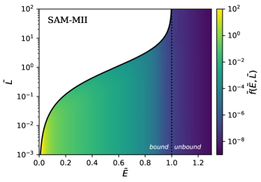
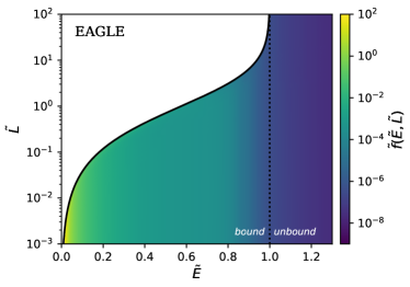
Figure 2: Dimensionless DFs $\tilde{f}(\tilde{E},\tilde{L})$ constructed from the SAM-MII (left) and EAGLE (right) simulations. The two DFs are quite similar, but the EAGLE DF has fewer tightly-bound (small $\tilde{E}$) satellites due to enhanced satellite disruption. The energy $\tilde{E}$ is always positive because the halo center is adopted as the zero point of the potential. Note that satellites with $\tilde{E}>1$ (to the right of the dotted line) are not bound. Note also that $f(E,L)$ is the DF in the 6D phase space of $\bm{r}$ and $\bm{v}$.

We expect that our DF has some dependence on the simulation used. In this work, we use template halo samples from two distinct simulations. For both samples, halos have the same mass range of $10^{11.5}\leq M/M_{\odot}\leq 10^{12.5}$, and their luminous satellites within $25r_{\mathrm{s}}$ are selected to construct the DF. One sample, the same as used in Li et al. (2019), is from the galaxy catalog generated by a semi-analytical model (SAM; Guo et al. 2011) based on the dark-matter-only simulation Millennium II (MII; Boylan-Kolchin et al. 2009). This sample contains $\sim\!10^{4}$ isolated halos with a total of $\sim\!10^{5}$ satellites, each having a stellar mass of $m_{\star}\geq 100\,M_{\odot}$. The other sample is selected from the hydrodynamics-based EAGLE Simulation (Schaye et al., 2015; Crain et al., 2015; McAlpine et al., 2016) with the same criteria as in Callingham et al. (2019) except for the halo mass range. This sample contains $\sim\!1700$ relaxed halos with a total of $\sim\!2.5\times 10^{4}$ satellites, each having at least one star particle. The concentration for the NFW profile of each halo is taken from Wang et al. (2017) for the MII simulation and Schaller et al. (2015) for the EAGLE simulation. For EAGLE halos, the concentration is fitted for the profile over $r=(0.05$–$1)R$.

The DFs $\tilde{f}(\tilde{E},\tilde{L})$ constructed from the SAM-MII and EAGLE simulations are shown in Figure 2. It can be seen that they are quite similar, but the EAGLE DF has fewer tightly-bound (small $\tilde{E}$) satellites. Using the same tests as for the SAM-MII DF in Li et al. (2019), we have checked that the EAGLE DF provides unbiased estimates of the mass and concentration for the underlying halo sample. In particular, as discussed in Appendix C, these estimates are insensitive to the presence of a massive neighbor or satellite like M31 or the Large Magellanic Cloud (LMC), respectively, for the MW. Comparing the results from the SAM-MII and EAGLE DFs allows us to assess the systematic uncertainties due to the simulation used. We will also show by the goodness-of-fit in Section 4.3 that the EAGLE simulation matches the observations better.

3.2 Estimating halo properties

Within the Bayesian statistical framework, we can use our DF to infer the halo mass $M$ and concentration $c$ efficiently and without bias. In addition, we can treat various observational effects, including the selection function (incompleteness) and measurement errors, in a rigorous and straightforward manner.

As discussed in Section 2, we consider only those MW satellites with $40<r<280\,\mathrm{kpc}$ and use an approximate selection function based on a luminosity-dependent completeness radius $R_{\mathrm{obs,max}}$ for each satellite. Consequently, the PDF including the selection function is

$$p_{\mathrm{s}}(\bm{w}|M,c)=\frac{f(\bm{w}|M,c)}{\int_{r_{\min}<r^{\prime}<\min\{r_{\max},R_{\mathrm{obs,max}}\}}f(\bm{w}^{\prime}|M,c)d^{6}\bm{w}^{\prime}},$$ (4)

where $r_{\min}=40\,\mathrm{kpc}$ and $r_{\max}=280\,\mathrm{kpc}$. Note that under our assumption of spherical symmetry, an angular selection function adds the same constant factor to both the numerator and the denominator, thus, having no effect on the above DF.

We further take observational errors into account through the hierarchical Bayesian technique, by integrating over all possible $\bm{w}$ corresponding to the observed $\hat{\bm{w}_{i}}$ for a satellite, to obtain

$$p_{\mathrm{ob}}(\hat{\bm{w}}_{i}|M,c)=\int p_{\mathrm{err}}(\hat{\bm{w}}_{i}|\bm{w})p_{\mathrm{s}}(\bm{w}|M,c)d^{6}\bm{w},$$ (5)

where $p_{\mathrm{err}}(\hat{\bm{w}}|{\bm{w}})$ describes the deviation of observables from their true values due to measurement errors. In practice, we use the Monte Carlo integration method to simplify the above calculation (e.g., Callingham et al. 2019). Specifically, for each satellite labeled $i$, we generate Monte Carlo realizations $\{\bm{w}_{ik}\}_{k=1,\,2,\cdots}$ that follow $p(\bm{w}_{ik})\propto p_{\mathrm{err}}(\hat{\bm{w}}_{i}|\bm{w}_{ik})$ (see Section 2.1) and take the average of $p_{\mathrm{s}}(\bm{w}_{ik}|M,c)$ for these realizations.

Using an observed sample of $n_{\mathrm{sat}}$ satellites with kinematic data $\{\hat{\bm{w}}_{i}\}_{i=1,\ldots,n_{\mathrm{sat}}}$, we can now infer the mass and concentration of the MW halo from the Bayesian formula

$$p(M,c|\{\hat{\bm{w}}_{i}\})=\frac{1}{Z}\left[{\textstyle\prod\nolimits^{n_{\mathrm{sat}}}_{i=1}}\,p_{\mathrm{ob}}({\hat{\bm{w}}}_{i}|M,c)\right]p(c|M)p(M),$$ (6)

where $p(M)$ and $p(c|M)$ represent our prior knowledge, and the normalization factor $Z$, also known as the Bayesian evidence, is given by integrating (marginalizing) the posterior (i.e., the expression after $1/Z$) over all possible model parameters $M$ and $c$. A model with a higher $Z$ is more favored as it gives a higher probability of obtaining the observational data (see e.g., Trotta 2008).

We use flat priors on both $\lg M$ and $\lg c$ by default to avoid relying on extra information. Based on cosmological simulations, the concentration for halos of the same mass follows a log-normal distribution with a scatter of $\sigma_{\lg c}\simeq 0.15\,\mathrm{dex}$ (Jing, 2000). Combining this result and the median $M$-$c$ relation derived from the EAGLE simulation (Schaller et al., 2015) gives an alternative prior on $\lg c$, which we take to be

$$p(\lg c|M)=\mathcal{N}\left(0.912-0.087\lg(M/10^{12}M_{\odot}),0.15\right).$$ (7)

Using the above prior or a similar one based on dark-matter-only simulations (e.g., Dutton & Macciò 2014) gives almost the same inferred halo properties.

4 Results

In this section, we apply our method to infer the MW halo properties based on the SAM-MII and EAGLE DFs, respectively, using the kinematic data for our sample of 28 satellites. We always use a flat prior on $\lg M$, but we present results for both a flat prior on $\lg c$ and the alternative prior [Equation (7)] based on the $M$-$c$ relation.

4.1 Halo mass and concentration

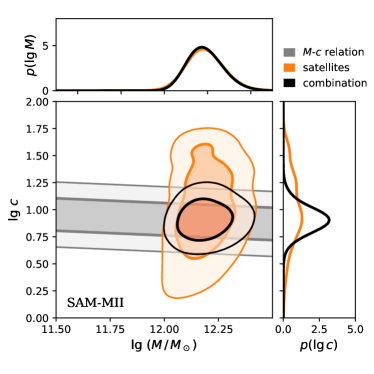
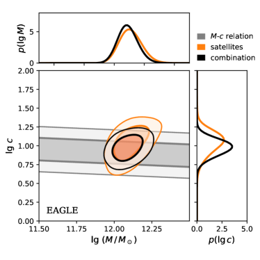
Figure 3: The MW halo mass and concentration inferred from the SAM-MII (left panel) and EAGLE (right panel) DFs. A flat prior on $\lg M$ is always used. Results are presented for both a flat prior on $\lg c$ (orange color) and the alternative prior (black color) based on the $M$-$c$ relation shown by the gray $1\sigma$ and $2\sigma$ contours. The other contours show the $1\sigma$ and $2\sigma$ confidence regions for the inferred $\lg M$ and $\lg c$. The corresponding marginalized distributions are shown in the upper and right subpanels.

Using the flat priors on $\lg M$ and $\lg c$, we calculate their joint probability distribution from Equation (6) on a 2D grid. The inferred $1\sigma$ (68.3%) and $2\sigma$ (95.4%) confidence regions are shown in Figure 3. The marginalized distributions of $\lg M$ and $\lg c$ are shown in the top and right subpanels, respectively, from which the marginalized $1\sigma$ confidence interval is obtained for each parameter. The above results are consistent with the $M$-$c$ relation. As expected, using the alternative prior based on this relation significantly reduces the uncertainty in the estimated $\lg c$, especially for the SAM-MII DF. However, because the inferred $\lg M$ depends on $\lg c$ only weakly, using the alternative prior improves the precision of the estimated $\lg M$ only slightly.

The best-fit values of $M$ and $c$ corresponding to the maximum posterior are listed in Table 1 along with the marginalized $1\sigma$ uncertainties. Parameters for the 2D Gaussian fit to the joint probability distribution of $\lg M$ and $\lg c$, including the mean and standard deviation of each variable and the correlation coefficient $\rho_{\mathrm{corr}}$, are also provided there for convenience of use. While the results from the SAM-MII and EAGLE DFs are consistent with each other at the $1\sigma$ level, the inferred halo mass is larger and has a larger statistical uncertainty for the SAM-MII DF. As shown in Section 4.3, the hydrodynamics-based EAGLE DF is significantly favored over the SAM-MII DF by the observations. Therefore, the results from the EAGLE DF are recommended. The enclosed mass $M(<r)$ within radius $r$ inferred from this DF is given for $r=30$–$400\,\mathrm{kpc}$ in Appendix B.

Table 1: Inferred MW halo mass and concentration. Results are presented for the SAM-MII and EAGLE DFs for a flat prior on $\lg c$ and the alternative prior based on the $M$-$c$ relation, as well as for combined tracer populations. Each set of results comprises the best-fit values of $M$ and $c$ with $1\sigma$ uncertainties, and the parameters for the 2D Gaussian fit to the joint probability distribution of $\lg M$ and $\lg c$, including the mean and standard deviation of each variable and the correlation coefficient $\rho_{\mathrm{corr}}$. The results from the EAGLE DF (in bold) are recommended.

	Satellites		Satellites + Halo Stars
	flat prior	$M$-$c$ relat.	flat prior	$M$-$c$ relat.
SAM-MII
$M^{\text{a}}$	$1.55_{-0.29}^{+0.35}$	$1.55_{-0.27}^{+0.33}$	$1.48_{-0.22}^{+0.26}$	$1.51_{-0.22}^{+0.26}$
$c$	$10.1_{-5.4}^{+11.6}$	$8.1_{-2.1}^{+2.8}$	$10.2_{-3.3}^{+4.8}$	$8.7_{-1.9}^{+2.4}$
$\lg\,M^{\text{a}}$	$0.19\pm 0.09$	$0.19\pm 0.08$	$0.17\pm 0.07$	$0.18\pm 0.07$
$\lg\,c$	$1.01\pm 0.33$	$0.91\pm 0.13$	$1.01\pm 0.17$	$0.94\pm 0.10$
$\rho_{\text{corr}}$	$0.24$	$0.10$	$-0.42$	$-0.26$
EAGLE
$M^{\text{a}}$	$1.29_{-0.20}^{+0.24}$	$\bm{1.23_{-0.18}^{+0.21}}$	$1.27_{-0.15}^{+0.17}$	$1.26_{-0.15}^{+0.17}$
$c$	$11.0_{-3.3}^{+4.8}$	$\bm{9.4_{-2.1}^{+2.8}}$	$11.7_{-2.5}^{+3.2}$	$10.4_{-1.9}^{+2.3}$
$\lg\,M^{\text{a}}$	$0.11\pm 0.07$	$\bm{0.09\pm 0.07}$	$0.10\pm 0.06$	$0.10\pm 0.06$
$\lg\,c$	$1.04\pm 0.16$	$\bm{0.97\pm 0.11}$	$1.07\pm 0.10$	$1.02\pm 0.09$
$\rho_{\text{corr}}$	$0.48$	$\bm{0.34}$	$0.06$	$0.05$
${}^{\text{a}}$ In units of $10^{12}M_{\odot}$ and including the baryonic contribution.

As our DF model is constructed to be the average DF for a sample of halos under a set of assumptions, individual halos are expected to deviate from the model in several aspects. For example, the mass distribution may deviate from a perfect spherical NFW profile, the satellites may be neither fully phase-mixed nor mutually independent due to the hierarchical accretion, and the scaled DF may not exactly follow our proposed form. The presence of massive satellites or companion galaxies, e.g., the LMC or M31 for our MW, might further increase the deviations (see more discussion below). All of these deviations can contribute to the halo-to-halo scatter in our mass estimates besides the statistical uncertainty. Using a large mock sample of realistic halos from the SAM-MII simulation, Li et al. (2019) estimated a systematic uncertainty of $\sim 7\%$ (0.03 dex) in $M$ when the prior based on the $M$-$c$ relation was used. It is worth emphasizing that given a realistic mock sample, all of the above halo-to-halo scatters should have already been captured by the above uncertainty. As discussed in Section 4.5, the dependence of our DF on the hydrodynamics-based simulations introduces an additional systematic uncertainty of $\sim 5\%$ in $M$. However, the above systematic uncertainties in $M$ are significantly smaller than the current statistical uncertainty of $\sim 17\%$ (see the relevant bold entry in Table 1).

4.2 Robustness of results

We now demonstrate the robustness of our results. For the EAGLE DF (see Appendix C), we find that the massive neighbor M31 has no significant influence on the inferred MW halo properties. The influence of the LMC might be more complicated. This massive satellite could imply a particular assembly history of the MW and induce non-trivial reflex motion of other satellites and the MW stellar halo (e.g., Petersen & Peñarrubia 2020; Erkal et al. 2020), thereby possibly causing bias in the MW mass estimate. Using a simplified test, Li et al. (2017) showed that adding a velocity offset of $30\,\mathrm{km\,s}^{-1}$ to the MW to mimic the reflex motion caused by the LMC only changes the results at a level $\lesssim 3\%$. Because the reflex motion is more complex than a simple bulk motion, it is better captured by our adopted simulations, which automatically include the effects due to massive satellites. As shown by the tests based on the simulations in Appendix C, the LMC has no significant influence on our MW mass estimate. Nevertheless, it is worth quantifying the effects of the LMC more precisely with a larger halo sample in the future. Below we present more tests and focus on the EAGLE DF with the prior based on the $M$-$c$ relation. The same tests for the SAM-MII DF give similar conclusions.

From a jackknife (leave-one-out) test on our sample of satellites, we find that the scatter in the inferred MW halo mass $M$ is comparable to the estimated statistical uncertainty in Table 1. In addition, the effect on the inferred $M$ is negligible compared to the statistical uncertainty when we exclude from our sample all of the possible LMC satellites: the Small Magellanic Cloud, Fornax, Carina I, and Horologium I (Kallivayalil et al., 2018; Pardy et al., 2020). Finally, as shown in Figure 4, we get remarkably consistent results on $M$ when varying the sample selection criteria based on the distance interval ($r_{\min},\ r_{\max}$), brightness ($m_{V,{\rm max}}$), or luminosity ($M_{V,{\rm max}}$) of the satellites. Note that varying $M_{V,\max}$ only changes the satellite sample, but the analysis remains the same as for the fiducial case. For the other tests, the $r_{\min}$, $r_{\max}$, and $R_{\mathrm{obs,max}}$ used in Equation (4) are changed accordingly. In particular, $R_{\mathrm{obs,max}}$ depends on $m_{V,{\rm max}}$.

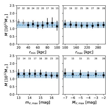
Figure 4: Robustness tests for the MW halo mass $M$ inferred from the EAGLE DF. In each panel, $r_{\min}$, $r_{\max}$, maximum apparent magnitude $m_{V,{\rm max}}$, or maximum absolute magnitude $M_{V,{\rm max}}$ for the satellite sample is changed from the fiducial value. For each sample, a filled square with an error bar shows the inferred $M$ with the $1\sigma$ uncertainty. The number of satellites, $n_{\mathrm{sat}}$, in each sample is indicated above the corresponding square. For reference, results (gray color) are also shown for two samples including satellites within $40\,\mathrm{kpc}$, which are beyond the scope intended for our method. The dashed line and the shaded band show the results for the fiducial sample ($n_{\mathrm{sat}}=28$, see Figure 1).

The robustness of our results demonstrated by the above tests can be attributed to two factors. First, the constraining power mainly comes from the bright satellites with precise measurements. Therefore, so long as a sample includes a sufficient number of such satellites, the inferred $M$ and its uncertainty should not change very much as the sample varies. More importantly, the robustness of our results also reflects the validity of our method, especially in treating the selection function and observational errors. Ignoring observational uncertainties overestimates the halo mass ($M\simeq 1.8\times 10^{12}M_{\odot}$) and gives an absurdly large concentration ($c\simeq 40$), while ignoring the selection function severely overestimates the concentration ($c\simeq 17$).

We emphasize that a rigorous and straightforward treatment of the selection function and observational errors is an important feature of the DF method. In contrast, it is rather difficult to treat observational errors in methods based on the Jeans equation. In some previous studies using such methods, because observational errors were not treated properly, including Leo I or not can change the estimated MW halo mass by $\sim 30\%$ (e.g., Watkins et al., 2010).

Another possible concern is the flattened satellite distribution of the MW, though its cosmological significance is still under debate (e.g., Pawlowski & Kroupa 2013; Cautun et al. 2015; Shao et al. 2019). However, the anisotropic distribution of satellites is unlikely able to bias our result significantly for two reasons. First, the mass estimate relies on the distance and velocity rather than the orbital orientation of a satellite. Second, as shown by the extensive tests in Li et al. (2019) and Appendix C, our method is robust for halos of a very wide range of halo structure, formation history and environment. Nevertheless, it is worth further investigating the peculiarities of the MW and their potential influence on the mass estimate.

4.3 Comparison of DFs with observations

For direct validation of the SAM-MII and EAGLE DFs, as well as the associated estimates of the MW halo properties, we compare these DFs with the observed satellite kinematics. For this purpose, we use the best-fit $M$ and $c$ inferred from each DF with the prior based on the $M$-$c$ relation. Under our assumptions, the DF $f({\bm{r}},{\bm{v}})$ can be written as $f(E,L)$, where $E$ and $L$ are functions of $r$, the radial velocity $v_{\mathrm{r}}$, and the tangential velocity $v_{\mathrm{t}}$ (see Section 3.1). Because it is difficult to show $f({\bm{r}},{\bm{v}})$ in the 3D space of $r$, $v_{\mathrm{r}}$, and $v_{\mathrm{t}}$, we instead display the projected DF in the 2D space of $r$ and $v_{\mathrm{t}}$ by marginalizing $v_{\mathrm{r}}$ and taking into account the selection function

$$p_{\mathrm{s}}(r,v_{\mathrm{t}})\propto 8\pi^{2}r^{2}v_{\mathrm{t}}N(<M_{V\!,\,\mathrm{lim}}(r))\int f({\bm{r}},{\bm{v}})dv_{\mathrm{r}},$$ (8)

where the factor $8\pi^{2}r^{2}v_{\mathrm{t}}$ comes from the differential phase-space volume element, $N(<M_{V})=10^{0.156M_{V}+2.21}$ is the complete satellite luminosity function derived by Newton et al. (2018), and $M_{V\!,\,\mathrm{lim}}(r)$ is the limiting absolute magnitude for Gaia proper motion measurement at radius $r$ [i.e., $r=R_{\mathrm{obs,max}}(M_{V\!,\,\mathrm{lim}}(r))$, see Section 2.2].

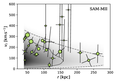
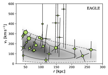
Figure 5: Comparison of the projected SAM-MII (left panel) and EAGLE (right panel) DFs with the observations. In each panel, $p_{\mathrm{s}}(r,v_{\mathrm{t}})$ with the best-fit $M$ and $c$ is shown as shades of gray (on the same intensity scale) along with the $1\sigma$ (solid) and $2\sigma$ (dashed) confidence contours. The data for our satellite sample are shown as circles, with larger ones indicating satellites with higher brightness. The error bars on each circle represent the axes of the $1\sigma$ error ellipse. See text for details.

Figure 5 shows $p_{\mathrm{s}}(r,v_{\mathrm{t}})$ for satellites with $40<r<280\,\mathrm{kpc}$ as shades of gray along with $1\sigma$ and $2\sigma$ confidence contours. Because the observational errors vary greatly among satellites, we have not included them in deriving $p_{\mathrm{s}}(r,v_{\mathrm{t}})$ for simplicity. Instead, we include these errors when showing the kinematic data for our satellite sample in Figure 5. Taking these errors into account when comparing the distribution of the data points with respect to the shades of gray and the confidence contours, we find that for both the SAM-MII and EAGLE DFs, the $2\sigma$ confidence region of $p_{\mathrm{s}}(r,v_{\mathrm{t}})$ with the best-fit $M$ and $c$ is consistent with the observations.

Figure 5 also shows that the EAGLE DF provides a significantly better match to the observations than the SAM-MII DF. Specifically, compared with the observations, the SAM-MII DF predicts a distribution of satellites that is too concentrated at smaller $r$ and $v_{\mathrm{t}}$. This discrepancy was also noticed for a similar halo sample based on the SAM-MII (Cautun & Frenk, 2017) or APOSTLE simulation suite (Riley et al., 2019). The above results are consistent with the ratio of the Bayesian evidence $Z$ [see Equation (6)] for the two DFs, which is also known as the Bayes factor. We find $Z(\mathrm{EAGLE})/Z(\mbox{SAM-MII})=33$ (or 25 when the flat prior on $\lg c$ is used), which indicates that the observations strongly favor the EAGLE DF. Therefore, the results from the EAGLE DF are recommended.

4.4 Inferring MW satellite kinematics

The orbits of satellites can shed important light on their past evolution and the assembly history of the MW. However, as shown in Figure 5, distant satellites typically have poorly measured proper motion, which makes it difficult to calculate their precise orbits. Having shown that the EAGLE DF provides a good description of the MW satellite kinematics, we can now use it to infer more precise velocities for those satellites with poor current measurements.

Given the kinematic data $\{\hat{\bm{w}}_{j}\}_{j=1,\ldots,n_{\mathrm{sat}}}$ for $n_{\mathrm{sat}}$ satellites, the posterior distribution of the true kinematics for the $i$th satellite is

$$\begin{split}p(\bm{w}_{i}|\{\hat{\bm{w}}_{j}\})\propto\int&p_{\mathrm{err}}(\hat{\bm{w}}_{i}|\bm{w}_{i})p_{\mathrm{s}}(\bm{w}_{i}|M,c)\\ \times&p(M,c|\{\hat{\bm{w}}_{j\neq i}\})dMdc,\end{split}$$ (9)

where $p(M,c|\{\hat{\bm{w}}_{j\neq i}\})$ is the distribution of halo parameters inferred from the data on all of the other satellites [see Equation (6)]. We calculate $p(\bm{w}_{i}|\{\hat{\bm{w}}_{j}\})$ using importance sampling. We first generate Monte Carlo realizations $\{\bm{w}_{ik}\}_{k=1,\,2,\cdots}$ with $p(\bm{w}_{ik})\propto p_{\mathrm{err}}(\hat{\bm{w}}_{i}|\bm{w}_{ik})$ (see Section 2.1). These $\bm{w}_{ik}$ along with the corresponding importance weight $\int p_{\mathrm{s}}(\bm{w}_{ik}|M,c)p(M,c|\{\hat{\bm{w}}_{j\neq i}\})dMdc$ represent the weighted realizations of $p(\bm{w}_{i}|\{\hat{\bm{w}}_{j}\})$, from which we can infer the best-fit values of $\bm{w}_{i}$ and the associated uncertainties.

The posterior satellite kinematic data inferred from Equation (9) are shown in Figure 6. It can be seen that the uncertainties in $v_{\mathrm{t}}$ are greatly reduced for those satellites with poor current measurements. As expected, the overall distribution of the posterior satellite kinematics also becomes very close to the projected DF $p_{\mathrm{s}}(r,v_{\mathrm{t}})$ (see Section 4.3). The posterior kinematic data are given in Appendix A, are available online at https://github.com/syrte/mw_sats_kin, and are archived in China-VO (doi:10.12149/101018).

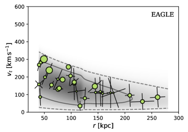
Figure 6: Same as the right panel of Figure 5, but showing the posterior satellite kinematics.

4.5 Dependence of the DF on cosmological simulations

Table 1 shows that the best-fit MW halo mass from the SAM-MII DF with the prior based on the $M$-$c$ relation is $\sim 26\%$ larger than that from the EAGLE DF. In addition, tests with mock samples of EAGLE halos show that the SAM-MII DF overestimates the halo mass by $\sim 12\%$ on average. Below, we discuss the underlying cause for the difference between these two DFs, which in turn gives rise to different estimates of halo properties.

The SAM-MII and EAGLE simulations differ in that the latter is based on hydrodynamics with baryonic physics. We consider that the full treatment of the stellar disk, including its gravitational effects, by the EAGLE simulation is most likely the main cause for the difference between the SAM-MII and EAGLE DFs. The stellar disk enhances the tidal field in the inner halo, thereby increasing the disruption rate for satellites with small pericenter distances $r_{\mathrm{peri}}$ (e.g., Garrison-Kimmel et al., 2017; Sawala et al., 2017; Richings et al., 2020). Because the formation and growth of the stellar disk were treated in the SAM-MII simulation without accounting for the associated change in the gravitational field, more satellites with small $r_{\mathrm{peri}}$ survived in this simulation compared to the EAGLE simulation and the MW observations. Consequently, satellites with small $r$ and $v_{\mathrm{t}}$, which also have small $r_{\mathrm{peri}}$, are over-represented by the SAM-MII DF (see Figure 5).

We find that the radial phase angle is uniformly distributed on average for satellites in both the SAM-MII (Li et al., 2019) and EAGLE simulations. So enhanced disruption by the stellar disk is more of a selection on orbit than on phase angle. Guided by this result, we mimic the gravitational effects of the stellar disk by manually increasing the disruption rate for satellites on orbits with small $r_{\mathrm{peri}}$ in the SAM-MII simulation. As shown in Figure 7, this prescription (see Appendix D) can give a projected DF $p_{\mathrm{s}}(r,v_{\mathrm{t}})$ very similar to that for the EAGLE simulation. Compared with $M=1.55_{-0.27}^{+0.33}\times 10^{12}\,M_{\odot}$ from the SAM-MII DF, the estimate from this modified SAM-MII DF, $M=1.35_{-0.19}^{+0.23}\times 10^{12}\,M_{\odot}$, is also much closer to $M=1.23_{-0.18}^{+0.21}\times 10^{12}\,M_{\odot}$ from the EAGLE DF.

While the hydrodynamics-based EAGLE simulation matches the observations better than the SAM-MII simulation, variation in the treatment of physical processes in current hydrodynamics-based simulations also leads to scatter in estimate of halo properties from the DF method. For example, compared to the APOSTLE simulation, the central galaxies in the Auriga simulation are more massive and, hence, more efficient at disrupting satellites. Consequently, the latter has approximately three times fewer surviving satellites within $0.1R$ than the former (Richings et al., 2020). Similar to the comparison of the EAGLE and SAM-MII DFs, the Auriga DF is expected to give lower halo mass estimates than the APOSTLE DF. This scatter in the halo mass estimate for DFs from hydrodynamics-based simulations should be much smaller than the difference of $\sim 12\%$ for the SAM-MII and EAGLE DFs. To better quantify this uncertainty, we vary the enhanced satellite disruption in the SAM-MII simulation according to the prescription in Appendix D, and obtain new satellite samples to construct modified SAM-MII DFs. Applying these DFs to EAGLE halos shows a scatter of only $\sim 5\%$ in the halo mass estimate (see Appendix D). We take this result as a reasonable estimate of the scatter for DFs from hydrodynamics-based simulations. This estimate is consistent with the findings of Callingham et al. (2019), who recovered halo masses in the Auriga simulation with little bias using the orbital distribution from the EAGLE simulation.

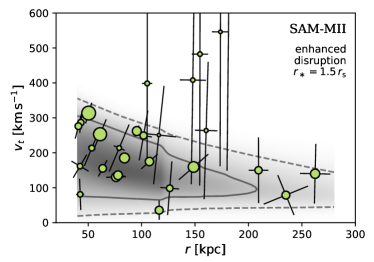
Figure 7: Same as the left panel of Figure 5, but for the modified SAM-MII DF based on enhanced disruption of satellites with small pericenter distances. See Appendix D for prescription of enhanced disruption using $r_{\ast}$.

5 Comparison with previous works and joint constraints

In this section, we compare the MW mass and its distribution inferred from the EAGLE DF with results from previous works. We also discuss possible improvement of our results by combining different tracer populations.

5.1 Comparison with previous results

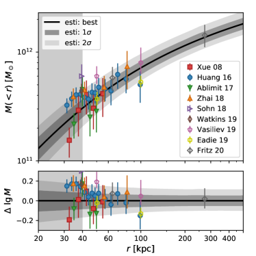
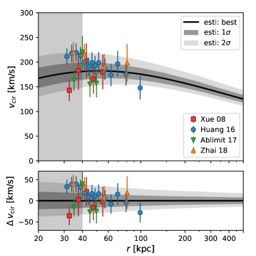
Figure 8: Comparison of the inferred mass profile (left panel) and rotation curve (right panel) for the MW outer halo with previous measurements (symbols with error bars). The black curves show the best-fit results from the EAGLE DF with the prior based on the $M$-$c$ relation, and the associated shaded bands are the $1\sigma$ and $2\sigma$ confidence regions. While our method focuses on the outer halo with $r>40\,\mathrm{kpc}$, our results should still be reliable inside but not too far from $r=40\,\mathrm{kpc}$.

Many studies were dedicated to measuring the halo mass and its distribution for the MW (for a comprehensive review, see Wang et al. 2019). In particular, much work focused on the rotation curve (RC) or masses enclosed within certain radii. A selected collection of recent measurements with halo stars (Xue et al., 2008; Huang et al., 2016; Ablimit & Zhao, 2017; Zhai et al., 2018), globular clusters (Sohn et al., 2018; Watkins et al., 2019; Vasiliev, 2019; Eadie & Jurić, 2019), and satellites (Fritz et al., 2020) beyond $r=40\,\mathrm{kpc}$ is shown in Figure 8. We convert the RC into the mass profile using $M(<r)=rv_{\mathrm{cir}}^{2}/G$ and vice versa. Here $M(<r)$ is the mass enclosed within radius $r$ and $v_{\mathrm{cir}}$ is the circular velocity at this $r$. Figure 8 also shows our results inferred from the EAGLE DF with the prior based on the $M$-$c$ relation for comparison (see Eadie & Jurić 2019 and Wang et al. 2019 for a more comprehensive comparison).

It can be seen from Figure 8 that our results are in good agreement with the RC measurements (within $1\sigma$ for most cases). Note that when multiple models of velocity anisotropy $\beta$ were used for an RC dataset, only those results assuming relatively high $\beta$ are shown based on the recent measurement of $\beta$ for halo stars with proper motion from Gaia (Bird et al., 2019). The low $\beta$ found in some earlier studies is likely due to e.g., contamination from the disk (McMillan, 2017) and substructures (Loebman et al., 2018).

We also note that studies using halo stars typically favor a smaller MW halo mass (e.g., $M\simeq 0.8\times 10^{12}M_{\odot}$ from Xue et al. 2008; Huang et al. 2016) and a higher concentration ($c\sim 14$–20, e.g., Deason et al., 2012; Kafle et al., 2014; Huang et al., 2016; Zhai et al., 2018). These differences from our results are likely due to the profile extrapolation to the outer halo used in these studies. For example, ignoring the contraction of dark matter profile in the inner halo would lead to biased profile extrapolation (Cautun et al., 2019). Because we use satellites, which are the proper tracers of the outer halo, the above issue is irrelevant for our results. Remarkably, our inferred mass profile is in very good agreement (within $\sim 0.5\sigma$) with the corresponding result of Cautun et al. (2019), who used both halo stars and satellites as tracers, and with that of Fritz et al. (2020), who applied the mass estimator of Watkins et al. (2010) to satellites within multiple radii.

5.2 Joint constraint with RC from halo stars

Combining different tracer populations on different spatial scales can improve the constraint on the MW mass profile. While the halo mass is mainly constrained by distant tracers like satellites, the nearby tracers serve as a better probe of the inner profile and, therefore, can improve the estimate of the halo concentration. In addition, if different tracer populations have independent systematics, combining them can reduce the systematic uncertainties. Examples of combining different tracer populations to constrain the MW halo properties include McMillan (2011, 2017) and Nesti & Salucci (2013) for using gas clouds, masers, and stars and Callingham et al. (2019) for using satellites and globular clusters.

For illustration, here we combine satellite kinematics with the RC from halo stars to constrain the MW halo mass and concentration. Using $\sim\!5,700$ halo K giants selected from the SDSS/SEGUE survey, Huang et al. (2016) derived the RC for the outer halo based on the spherical Jeans equation. While their data could benefit from a reanalysis using an updated $\beta$ from Gaia, these data are currently the best for relatively large radii. We only use their data for $40<r<80\,\mathrm{kpc}$ (see the right panel of Figure 8). An important issue is the treatment of the relevant uncertainties. In addition to the measurement uncertainty $\sigma_{v_{\mathrm{cir},i}}$ in the circular velocity $v_{\mathrm{cir},i}$ at radius $r_{i}$, there is an additional large systematic uncertainty from the assumed power-law index $\alpha$ for the stellar density profile in the outer halo. Huang et al. (2016) adopted $\alpha=-4.5$ as the fiducial value. However, current observations allow $\alpha=-3.8$ to $-5$ and variation over this range systematically changes the derived $v_{\mathrm{cir},i}$ at the level of $\sigma_{\mathrm{sys}}=15\,\mathrm{km\,s}^{-1}$ (see Huang et al. 2016 for detailed discussion). Therefore, the RC measurements at different radii are not independent. Ignoring this correlation of measurements, as usually done in previous studies, leads to underestimated formal errors. A proper treatment is to use the covariance matrix

$$\mathcal{M}_{ij}=\mathrm{cov}\!\left(v_{\mathrm{cir},i},\,v_{\mathrm{cir},j}\right)=\Bigg{\{}\begin{aligned} &\sigma_{v_{\mathrm{cir},i}}^{2}+\sigma_{\mathrm{sys}}^{2},&i=j,\\ &\sigma_{\mathrm{sys}}^{2},&i\neq j.\end{aligned}$$ (10)

The RC data can be modeled as a multivariate Gaussian distribution. For a specific set of $M$ and $c$ for the NFW profile, the expected $v_{\mathrm{cir}}$ at radius $r_{i}$ is $v_{\mathrm{cir}}(r_{i}|M,c)=\sqrt{GM_{\mathrm{NFW}}(<r_{i}|M,c)/r_{i}}$. The probability (likelihood) of $n$ measurements $\{v_{\mathrm{cir},i}\}_{i=1,2,\ldots,n}$ is

$$p(\left\{v_{\mathrm{cir},i}\right\}|M,c)=\frac{\exp\!\big{[}-\!\frac{1}{2}\sum_{i,j}\Delta v_{i}(\mathcal{M}^{-1})_{ij}\Delta v_{j}\big{]}}{\sqrt{(2\pi)^{n}\det(\mathcal{M})}},$$ (11)

where $\Delta v_{i}=v_{\mathrm{cir},i}-v_{\mathrm{cir}}(r_{i}|M,c)$. The above likelihood can be used independently, or multiplied by the likelihood in Equation (6) for joint analysis.

Figure 9 shows the MW halo parameters inferred using (1) the RC from halo stars, (2) the EAGLE DF for satellite kinematics with a flat prior on $\lg c$, and (3) a combination of (1) and the EAGLE DF with the prior based on the $M$-$c$ relation. It can be seen that while the constraints on $\lg M$ and $\lg c$ from (1) are rather loose, they are approximately orthogonal to those from (2). In addition, the overlap of these two sets of constraints is in remarkable agreement with the $M$-$c$ relation (here taken from the EAGLE simulation but similar to those from other simulations), which nicely illustrates how the best constraints are obtained using (3). For numerical results, by combining the RC from halo stars with satellite kinematics, we obtain $M=1.27_{-0.15}^{+0.17}\times 10^{12}M_{\odot}$ and $c=11.7_{-2.5}^{+3.2}$ ($M=1.26_{-0.15}^{+0.17}\times 10^{12}M_{\odot}$ and $c=10.4_{-1.9}^{+2.3}$) for a flat prior on $\lg c$ (the prior based on the $M$-$c$ relation), to be compared with $M=1.29_{-0.20}^{+0.24}\times 10^{12}M_{\odot}$ and $c=11.0_{-3.3}^{+4.8}$ ($M=1.23_{-0.18}^{+0.21}\times 10^{12}M_{\odot}$ and $c=9.4_{-2.1}^{+2.8}$) from satellite kinematics alone (see Table 1). The joint constraints only slightly improve the precision of $M$ because satellites are the best tracers of halo mass. On the other hand, when a flat prior on $\lg c$ is used, the joint constraints significantly improve the precision of $c$ due to additional constraints from halo stars on the inner profile. Effectively, the joint constraints remove the need for the prior based on the $M$-$c$ relation.

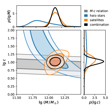
Figure 9: Similar to the right panel of Figure 3, but showing additional results obtained using the RC from halo stars. The blue (orange) contours show the 1 $\sigma$ and 2 $\sigma$ confidence regions inferred using only the RC from halo stars (satellite kinematics with a flat prior on $\lg c$). The black contours show the results obtained by combining the RC from halo stars and satellite kinematics with the prior based on the $M$-$c$ relation (shown as the gray contours). See text for details.

Clearly, the gain from adding a tracer population increases with the precision of the relevant data and the understanding of the potential systematics. The use of halo stars as tracers will certainly benefit from Gaia and its future data release, as well as other ongoing spectroscopic surveys. These programs can reach further into the outer halo, and more importantly, they can get rid of the mass-anisotropy degeneracy and reduce the substructure contamination (e.g., Bird et al. 2019) by directly measuring 3D velocities of halo stars.

6 Summary and Conclusions

We have estimated the mass and concentration of the MW halo using the kinematic data on its satellite galaxies, including the latest measurements from Gaia DR2. Using realistic 6D phase-space DFs of satellite kinematics constructed from cosmological simulations, we can infer the halo properties efficiently and without bias, and handle the selection function and measurement errors rigorously in the Bayesian framework. Applying our DF from the EAGLE simulation to 28 satellites, we obtain an MW halo mass of $M=1.23_{-0.18}^{+0.21}\times 10^{12}M_{\odot}$ and a concentration of $c=9.4_{-2.1}^{+2.8}$ with the prior based on the $M$-$c$ relation. The systematic uncertainties in $M$ due to halo-to-halo scatter ($\sim\!7\%$) and to differences among hydrodynamics-based simulations ($\sim\!5\%$) are small compared to the current statistic error ($\sim\!17\%$). Due to proper treatment of observational effects, our results are insensitive to sample selection. In addition, they seem robust against the massive neighbor M31 or the massive satellite LMC. We recommend the above results as currently the best estimates of the MW mass and its profile in the outer halo.

Our MW mass estimate is consistent with the latest estimates from various tracers (e.g., Zhai et al. 2018; Sohn et al. 2018; Watkins et al. 2019; Vasiliev 2019; Cautun et al. 2019; Fritz et al. 2020, see also the review by Wang et al. 2019) and, in particular, with those using satellite orbital distributions from simulations (Li et al., 2017; Patel et al., 2018; Callingham et al., 2019). However, our estimate is more precise and reliable due to the improved methodology and data.

Our mass estimate is also in good agreement with the estimates from the escape velocity of halo stars (e.g., Deason et al. 2019; Grand et al. 2019) and the timing argument with halo stars (Zaritsky et al., 2020) or nearby galaxies (Peñarrubia et al. 2016; Peñarrubia & Fattahi 2017), which represent completely different approaches to deriving the mass.

In addition, our inferred MW mass profile is consistent with previous measurements using halo stars (Xue et al., 2008; Huang et al., 2016; Ablimit & Zhao, 2017; Zhai et al., 2018), globular clusters (Sohn et al., 2018; Watkins et al., 2019; Vasiliev, 2019; Eadie & Jurić, 2019), and satellite galaxies (Cautun et al., 2019; Fritz et al., 2020). Studies using the RC of halo stars usually gave smaller MW mass estimates, most likely due to biased profile extrapolation to the outer halo. For example, ignoring the contraction of dark matter profile in the inner halo would lead to biased profile extrapolation (Cautun et al., 2019). Because satellites are the proper tracers of the outer halo, the above issue is irrelevant for our results. Halo stars are also expected to have larger intrinsic systematics due to the larger deviation from steady state compared to satellites (e.g., Wang et al., 2017, 2018; Han et al., 2019).

We have also presented results from the SAM-MII DF based on a dark-matter-only simulation. By comparing both this DF and the EAGLE DF with the observations, we have shown that the hydrodynamics-based EAGLE simulation provides a better description of MW satellite kinematics. Using the EAGLE DF and the associated best-fit MW potential, we have provided much more precise estimates of kinematics for those satellites with uncertain measurements, which may help to better understand their past evolution and the assembly history of the MW.

By comparing the SAM-MII and EAGLE DFs, we find that the former over-represents satellites with small radii and velocities, most likely because the gravitational effects of the stellar disk were not accounted for in the SAM-MII simulation. Such effects include the enhancement of the tidal field and hence the disruption rate for satellites with small pericenter distances $r_{\mathrm{peri}}$. The inadequate satellite disruption is likely the main cause of the earlier reported discrepancy in the velocity anisotropy between the MW satellite system and the SAM-MII (Cautun & Frenk, 2017) or APOSTLE simulation suite (Riley et al., 2019). We have shown that the differences among hydrodynamics-based simulations may be mimicked by prescribing the satellite disruption rate as a function of $r_{\mathrm{peri}}$ in the SAM-MII simulation, which allows us to estimate the scatter ($\sim\!5\%$) of halo mass estimates from different hydrodynamics-based simulations.

In the future, the ongoing and planned surveys will increase both the number of tracers in different populations and the quality of the relevant data, which in turn, will enable us to determine the MW halo properties with increasing accuracy. For example, the number of known satellites may eventually increase by a factor of $\sim 2$–10 (Simon, 2019). The statistical uncertainty decreases as $1/\sqrt{n_{\mathrm{sat}}}$, and becomes comparable to the systematic uncertainty when the number of satellites with complete kinematic data reaches $n_{\mathrm{sat}}\sim 100$ (Li et al., 2019). Ultimately, a better understanding of the particular MW formation history and its influence on the mass estimate is required to reduce the systematics. Note that whereas we have selected the satellites with full kinematic data for convenience of analysis in this study, our method can treat satellites with incomplete data as well (Li et al., 2019). In addition, if different tracer populations have independent systematics, combining multiple tracer populations can further improve the precision by reducing the systematic uncertainties. As an illustration, we have combined the RC from halo stars with satellite kinematics to demonstrate the potential of this approach to improve estimates of halo properties. Because halo stars and satellites probe different regions of the outer halo, their combined use effectively removes the need for the prior based on the $M$-$c$ relation.

Compared to satellites, stars and stellar clusters are currently less well understood due to limited resolution and various model uncertainties of the simulations. Nevertheless, when we have the proper simulations for these tracers, our simulation-based DF method can also apply to e.g., halo stars or globular clusters. In general, the quality of any DF can be judged based on the Bayesian evidence or a direct comparison of the DF with the observed tracer kinematics. On the other hand, non-parametric methods (e.g., Bovy et al., 2010; Magorrian, 2014; Han et al., 2016b), which suffer less from model assumptions, might be attractive alternatives for dynamical modeling of halo stars or globular clusters when more and better data are available.

Appendix A MW satellite properties and posterior kinematics

Table 2 lists the observed properties of those MW satellites used in our study, including the coordinates, absolute magnitude, distance, line-of-sight velocity, and proper motion. They are taken from Table A1 (gold sample when possible) of the compilation by Riley et al. (2019). Two additional entries list the posterior proper motion estimates derived from our EAGLE DF with the prior based on the $M$-$c$ relation (see Section 4.4).

Table 3 lists the Galactocentric position and velocity, as well as the corresponding uncertainties, obtained by Monte Carlo sampling for each satellite (see Section 2.1 for detail). Four additional entries list the posterior kinematics derived in Section 4.4. These values are listed for reference. We recommend that readers of interest instead use the Monte Carlo sample and the corresponding importance weights, which are available online at https://github.com/syrte/mw_sats_kin and are archived in China-VO (doi:10.12149/101018).

=5.3cm

Table 2: Properties of the satellites used in this study: RA ($\alpha$), Dec ($\delta$), absolute magnitude, heliocentric distance, line-of-sight velocity, and proper motion. They are taken from a compilation by Riley et al. (2019). References for original observations are also given. The last two columns list our posterior proper motion estimates. Note that $\mu_{\alpha^{\ast}}\equiv\mu_{\alpha}\cos\delta$.

Satellite	RA	Dec	$M_{V}$	$D_{\odot}$	$v_{\odot}$	$\mu_{\alpha^{\ast}}$	$\mu_{\delta}$	Reference	$\mu_{\alpha^{\ast}}^{\mathrm{post}}$	$\mu_{\delta}^{\mathrm{post}}$
	[deg]	[deg]	[mag]	[$\mathrm{kpc}$]	[$\mathrm{km\,s}^{-1}$]	[$\mathrm{mas\,yr}^{-1}$]	[$\mathrm{mas\,yr}^{-1}$]		[$\mathrm{mas\,yr}^{-1}$]	[$\mathrm{mas\,yr}^{-1}$]
Aquarius II	$338.481$	$-9.327$	$-4.36$	$107.9\pm 3.3$	$-71.1\pm 2.5$	$-0.491\pm 0.306$	$-0.049\pm 0.266$	[7, 1]	$-0.098_{-0.131}^{+0.164}$	$-0.223_{-0.191}^{+0.127}$
Bootes I	$210.015$	$14.512$	$-6.3$	$66\pm 3$	$102.2\pm 0.8$	$-0.459\pm 0.041$	$-1.064\pm 0.029$	[8, 9, 10, 2]	$-0.460_{-0.042}^{+0.043}$	$-1.063_{-0.029}^{+0.028}$
Canes Venatici I	$202.016$	$33.559$	$-8.6$	$210\pm 6$	$30.9\pm 0.6$	$-0.159\pm 0.1$	$-0.067\pm 0.064$	[9, 11, 12, 3]	$-0.159_{-0.063}^{+0.062}$	$-0.113_{-0.053}^{+0.047}$
Canes Venatici II	$194.292$	$34.321$	$-4.6$	$160\pm 7$	$-128.9\pm 1.2$	$-0.342\pm 0.238$	$-0.473\pm 0.178$	[12, 13, 14, 3]	$-0.227_{-0.097}^{+0.125}$	$-0.333_{-0.103}^{+0.096}$
Carina I	$100.407$	$-50.966$	$-8.6$	$105.6\pm 5.4$	$222.9\pm 0.1$	$0.495\pm 0.015$	$0.143\pm 0.014$	[15, 16, 17, 2]	$0.493_{-0.014}^{+0.016}$	$0.143_{-0.014}^{+0.013}$
Coma Berenices I	$186.746$	$23.908$	$-3.8$	$42\pm 1.5$	$98.1\pm 0.9$	$0.546\pm 0.092$	$-1.726\pm 0.086$	[12, 18, 19, 4]	$0.522_{-0.091}^{+0.093}$	$-1.711_{-0.089}^{+0.083}$
Crater II	$177.31$	$-18.413$	$-8.2$	$117.5\pm 1.1$	$87.5\pm 0.4$	$-0.246\pm 0.052$	$-0.227\pm 0.026$	[20, 21, 1]	$-0.247_{-0.052}^{+0.050}$	$-0.226_{-0.025}^{+0.025}$
Draco I	$260.06$	$57.965$	$-8.75$	$76\pm 6$	$-291\pm 0.1$	$-0.019\pm 0.009$	$-0.145\pm 0.01$	[22, 23, 2]	$-0.019_{-0.009}^{+0.009}$	$-0.145_{-0.010}^{+0.010}$
Fornax	$39.962$	$-34.511$	$-13.4$	$147\pm 9$	$55.3\pm 0.1$	$0.376\pm 0.003$	$-0.413\pm 0.003$	[17, 24, 2]	$0.376_{-0.003}^{+0.003}$	$-0.413_{-0.003}^{+0.003}$
Grus I	$344.176$	$-50.163$	$-3.4$	$120.2\pm 11.1$	$-140.5\pm 2$	$-0.25\pm 0.16$	$-0.47\pm 0.23$	[25, 26, 5]	$-0.045_{-0.101}^{+0.106}$	$-0.453_{-0.129}^{+0.142}$
Hercules	$247.763$	$12.787$	$-6.6$	$132\pm 6$	$45.2\pm 1.09$	$-0.297\pm 0.123$	$-0.329\pm 0.1$	[27, 28, 3]	$-0.284_{-0.098}^{+0.103}$	$-0.314_{-0.084}^{+0.087}$
Horologium I	$43.882$	$-54.119$	$-3.5$	$79\pm 7$	$112.8\pm 2.55$	$0.95\pm 0.07$	$-0.55\pm 0.06$	[29, 5]	$0.935_{-0.070}^{+0.069}$	$-0.542_{-0.058}^{+0.057}$
Hydra II	$185.425$	$-31.985$	$-4.8$	$151\pm 8$	$303.1\pm 1.4$	$-0.417\pm 0.402$	$0.179\pm 0.339$	[30, 31, 32, 1]	$-0.228_{-0.115}^{+0.162}$	$-0.094_{-0.112}^{+0.114}$
Leo I	$152.122$	$12.313$	$-12.03$	$258.2\pm 9.5$	$282.5\pm 0.1$	$-0.097\pm 0.056$	$-0.091\pm 0.047$	[33, 34, 2]	$-0.071_{-0.039}^{+0.041}$	$-0.123_{-0.037}^{+0.035}$
Leo II	$168.37$	$22.152$	$-9.6$	$233\pm 15$	$78.5\pm 0.6$	$-0.064\pm 0.057$	$-0.21\pm 0.054$	[35, 36, 2]	$-0.071_{-0.046}^{+0.045}$	$-0.207_{-0.045}^{+0.046}$
Leo IV	$173.233$	$-0.54$	$-4.97$	$154\pm 5$	$132.3\pm 1.4$	$-0.59\pm 0.534$	$-0.449\pm 0.362$	[12, 37, 3]	$-0.157_{-0.145}^{+0.125}$	$-0.270_{-0.147}^{+0.135}$
Leo V	$172.784$	$2.222$	$-4.4$	$173\pm 5$	$172.1\pm 2.2$	$-0.097\pm 0.56$	$-0.628\pm 0.307$	[38, 39, 3]	$-0.128_{-0.093}^{+0.096}$	$-0.272_{-0.101}^{+0.125}$
LMC	$80.894$	$-69.756$	$-18.1$	$51\pm 2$	$262.2\pm 3.4$	$1.85\pm 0.03$	$0.24\pm 0.03$	[40, 2]	$1.845_{-0.031}^{+0.031}$	$0.241_{-0.030}^{+0.027}$
Pisces II	$344.634$	$5.955$	$-4.1$	$183\pm 15$	$-226.5\pm 2.7$	$-0.108\pm 0.647$	$-0.586\pm 0.502$	[14, 30, 3]	$0.096_{-0.101}^{+0.113}$	$-0.215_{-0.093}^{+0.111}$
Sculptor	$15.039$	$-33.709$	$-10.7$	$83.9\pm 1.5$	$111.4\pm 0.1$	$0.082\pm 0.005$	$-0.131\pm 0.004$	[17, 41, 2]	$0.082_{-0.005}^{+0.005}$	$-0.131_{-0.004}^{+0.004}$
Segue 2	$34.817$	$20.175$	$-2.5$	$36.6\pm 2.45$	$-40.2\pm 0.9$	$1.01\pm 0.14$	$-0.48\pm 0.18$	[42, 43, 6]	$1.002_{-0.149}^{+0.152}$	$-0.447_{-0.203}^{+0.194}$
Sextans	$153.268$	$-1.62$	$-9.3$	$92.5\pm 2.2$	$224.2\pm 0.1$	$-0.496\pm 0.025$	$0.077\pm 0.02$	[17, 44, 2]	$-0.490_{-0.024}^{+0.025}$	$0.072_{-0.021}^{+0.019}$
SMC	$13.187$	$-72.829$	$-16.8$	$64\pm 4$	$145.6\pm 0.6$	$0.797\pm 0.03$	$-1.22\pm 0.03$	[40, 2]	$0.796_{-0.030}^{+0.028}$	$-1.214_{-0.031}^{+0.030}$
Tucana II	$343.06$	$-58.57$	$-3.9$	$57.5\pm 5.3$	$-129.1\pm 3.5$	$0.91\pm 0.06$	$-1.16\pm 0.08$	[26, 45, 5]	$0.905_{-0.059}^{+0.058}$	$-1.152_{-0.079}^{+0.075}$
Ursa Major I	$158.685$	$51.926$	$-6.75$	$97.3\pm 5.85$	$-55.3\pm 1.4$	$-0.659\pm 0.093$	$-0.635\pm 0.131$	[12, 46, 4]	$-0.590_{-0.080}^{+0.084}$	$-0.616_{-0.112}^{+0.114}$
Ursa Major II	$132.874$	$63.133$	$-3.9$	$34.7\pm 2.1$	$-116.5\pm 1.9$	$1.661\pm 0.053$	$-1.87\pm 0.065$	[12, 47, 4]	$1.656_{-0.052}^{+0.052}$	$-1.868_{-0.066}^{+0.065}$
Ursa Minor	$227.242$	$67.222$	$-8.4$	$76\pm 4$	$-246.9\pm 0.1$	$-0.182\pm 0.01$	$0.074\pm 0.008$	[48, 2]	$-0.181_{-0.010}^{+0.010}$	$0.074_{-0.008}^{+0.008}$
Willman 1	$162.341$	$51.053$	$-2.7$	$38\pm 7$	$-12.8\pm 1$	$0.382\pm 0.119$	$-1.152\pm 0.216$	[9, 49, 4]	$0.372_{-0.117}^{+0.117}$	$-1.167_{-0.203}^{+0.210}$

References. [1] Kallivayalil et al. (2018); [2] Gaia Collaboration et al. (2018b); [3] Fritz et al. (2018); [4] Simon (2018); [5] Pace & Li (2019); [6] Massari & Helmi (2018); [7] Torrealba et al. (2016b); [8] Dall’Ora et al. (2006); [9] Martin et al. (2008); [10] Koposov et al. (2011); [11] Kuehn et al. (2008); [12] Simon & Geha (2007); [13] Greco et al. (2008); [14] Sand et al. (2012); [15] Karczmarek et al. (2015); [16] McMonigal et al. (2014); [17] Walker et al. (2009); [18] Muñoz et al. (2010); [19] Musella et al. (2009); [20] Caldwell et al. (2017); [21] Torrealba et al. (2016a); [22] Walker et al. (2015); [23] Bonanos et al. (2004); [24] Pietrzyński et al. (2009); [25] Koposov et al. (2015a); [26] Walker et al. (2016); [27] Adén et al. (2009); [28] Musella et al. (2012); [29] Koposov et al. (2015b); [30] Kirby et al. (2015); [31] Vivas et al. (2016); [32] Martin et al. (2015); [33] Mateo et al. (2008); [34] Stetson et al. (2014); [35] Spencer et al. (2017); [36] Bellazzini et al. (2005); [37] Moretti et al. (2009); [38] Collins et al. (2017); [39] Medina et al. (2017); [40] McConnachie (2012); [41] Martínez-Vázquez et al. (2015); [42] Boettcher et al. (2013); [43] Kirby et al. (2013); [44] Okamoto et al. (2017); [45] Bechtol et al. (2015); [46] Garofalo et al. (2013); [47] Dall’Ora et al. (2012); [48] Bellazzini et al. (2002); [49] Willman et al. (2011).

=5.3cm

Table 3: Galactocentric positions and velocities of the satellites. The last four columns list our estimated posterior kinematics. All values are in terms of the median and the $1\sigma$ uncertainty.

Satellite	$r$	$\theta$	$\phi$	$v_{r}$	$v_{\theta}$	$v_{\phi}$	$r^{\mathrm{post}}$	$v^{\mathrm{post}}_{r}$	$v^{\mathrm{post}}_{\theta}$	$v^{\mathrm{post}}_{\phi}$
	[kpc]	[deg]	[deg]	[$\mathrm{km\,s}^{-1}$]	[$\mathrm{km\,s}^{-1}$]	[$\mathrm{km\,s}^{-1}$]	[$\mathrm{kpc}$]	[$\mathrm{km\,s}^{-1}$]	[$\mathrm{km\,s}^{-1}$]	[$\mathrm{km\,s}^{-1}$]
Aquarius II	$105.3_{-3.5}^{+3.2}$	$145.0_{-0.1}^{+0.1}$	$61.7_{-0.2}^{+0.2}$	$34.2_{-11.4}^{+11.7}$	$-372.1_{-145.4}^{+152.8}$	$-62.5_{-138.8}^{+146.8}$	$105.0_{-3.3}^{+3.4}$	$44.4_{-6.7}^{+6.9}$	$-149.0_{-55.4}^{+94.3}$	$-6.4_{-91.2}^{+88.3}$
Bootes I	$63.7_{-2.9}^{+2.9}$	$13.6_{-0.3}^{+0.3}$	$357.1_{-0.1}^{+0.1}$	$95.8_{-1.6}^{+1.7}$	$123.1_{-12.2}^{+11.9}$	$-94.8_{-19.7}^{+19.7}$	$63.5_{-2.9}^{+2.9}$	$95.8_{-1.6}^{+1.6}$	$122.7_{-12.0}^{+11.9}$	$-93.5_{-19.5}^{+19.1}$
Canes Venatici I	$210.0_{-6.1}^{+5.9}$	$9.8_{-0.0}^{+0.0}$	$86.0_{-0.4}^{+0.4}$	$83.3_{-3.4}^{+3.6}$	$89.2_{-81.2}^{+82.7}$	$76.2_{-83.2}^{+88.9}$	$209.6_{-6.5}^{+5.7}$	$82.2_{-2.3}^{+2.3}$	$53.1_{-54.9}^{+57.7}$	$46.6_{-56.5}^{+57.5}$
Canes Venatici II	$160.6_{-6.8}^{+7.0}$	$8.8_{-0.1}^{+0.1}$	$130.4_{-0.6}^{+0.6}$	$-93.3_{-8.9}^{+9.2}$	$-144.0_{-142.8}^{+136.8}$	$134.3_{-182.3}^{+187.0}$	$158.6_{-6.3}^{+7.5}$	$-94.2_{-4.1}^{+4.3}$	$-47.3_{-71.5}^{+74.2}$	$39.1_{-93.3}^{+69.4}$
Carina I	$107.5_{-5.3}^{+5.1}$	$111.8_{-0.0}^{+0.0}$	$255.4_{-0.2}^{+0.2}$	$-4.2_{-0.6}^{+0.5}$	$-173.0_{-14.1}^{+14.8}$	$-27.4_{-7.0}^{+6.8}$	$106.1_{-5.1}^{+5.1}$	$-4.1_{-0.6}^{+0.5}$	$-169.2_{-14.1}^{+15.2}$	$-27.4_{-7.0}^{+6.6}$
Coma Berenices I	$43.2_{-1.5}^{+1.5}$	$14.8_{-0.3}^{+0.4}$	$201.8_{-0.6}^{+0.6}$	$26.5_{-3.6}^{+3.5}$	$-265.9_{-19.6}^{+18.3}$	$103.3_{-21.3}^{+22.5}$	$43.0_{-1.4}^{+1.5}$	$27.3_{-3.5}^{+3.4}$	$-261.3_{-19.4}^{+17.5}$	$99.6_{-21.0}^{+22.7}$
Crater II	$116.4_{-1.1}^{+1.1}$	$47.5_{-0.0}^{+0.0}$	$277.7_{-0.1}^{+0.1}$	$-83.7_{-1.9}^{+1.9}$	$-1.7_{-16.3}^{+17.8}$	$-30.6_{-27.0}^{+26.5}$	$116.4_{-1.1}^{+1.1}$	$-83.7_{-1.9}^{+1.9}$	$-1.7_{-16.2}^{+17.8}$	$-30.5_{-27.2}^{+26.4}$
Draco I	$76.2_{-6.1}^{+6.0}$	$55.3_{-0.0}^{+0.0}$	$93.8_{-0.6}^{+0.7}$	$-88.0_{-0.4}^{+0.4}$	$122.4_{-3.4}^{+3.2}$	$-45.7_{-6.1}^{+5.2}$	$75.8_{-6.2}^{+6.0}$	$-88.0_{-0.4}^{+0.4}$	$122.4_{-3.4}^{+3.2}$	$-45.4_{-6.1}^{+5.2}$
Fornax	$149.0_{-9.1}^{+8.9}$	$153.9_{-0.1}^{+0.1}$	$230.9_{-0.4}^{+0.3}$	$-41.2_{-0.2}^{+0.2}$	$-106.3_{-18.0}^{+18.1}$	$120.3_{-15.9}^{+15.9}$	$144.4_{-8.1}^{+8.4}$	$-41.2_{-0.1}^{+0.2}$	$-97.0_{-16.9}^{+15.9}$	$112.0_{-14.6}^{+15.1}$
Grus I	$115.9_{-10.7}^{+11.4}$	$151.6_{-0.3}^{+0.3}$	$335.5_{-0.4}^{+0.3}$	$-202.7_{-6.2}^{+5.9}$	$-183.7_{-115.3}^{+102.6}$	$109.5_{-122.3}^{+117.1}$	$110.1_{-11.0}^{+11.3}$	$-195.6_{-4.2}^{+3.7}$	$-84.4_{-53.3}^{+63.4}$	$51.0_{-75.5}^{+70.8}$
Hercules	$126.3_{-5.8}^{+6.0}$	$51.3_{-0.1}^{+0.1}$	$30.9_{-0.1}^{+0.1}$	$150.6_{-3.3}^{+3.0}$	$-11.4_{-71.2}^{+74.1}$	$-56.9_{-63.5}^{+66.1}$	$125.5_{-5.8}^{+5.8}$	$150.8_{-2.8}^{+2.6}$	$-3.8_{-61.2}^{+60.5}$	$-43.3_{-52.3}^{+57.0}$
Horologium I	$79.4_{-6.5}^{+6.6}$	$144.4_{-0.1}^{+0.1}$	$260.9_{-0.9}^{+0.8}$	$-32.5_{-3.5}^{+3.5}$	$-212.5_{-42.5}^{+41.2}$	$-8.0_{-23.8}^{+22.9}$	$75.8_{-6.0}^{+6.2}$	$-32.6_{-3.5}^{+3.6}$	$-187.3_{-36.7}^{+32.5}$	$-6.9_{-22.8}^{+21.2}$
Hydra II	$148.2_{-8.0}^{+8.2}$	$58.9_{-0.0}^{+0.0}$	$292.4_{-0.2}^{+0.2}$	$130.6_{-15.5}^{+14.3}$	$-194.2_{-243.7}^{+235.0}$	$-214.0_{-278.7}^{+299.8}$	$146.1_{-6.6}^{+8.4}$	$119.5_{-6.2}^{+4.1}$	$-30.3_{-81.0}^{+81.0}$	$-21.7_{-81.9}^{+103.6}$
Leo I	$262.1_{-9.1}^{+9.3}$	$41.7_{-0.0}^{+0.0}$	$224.2_{-0.1}^{+0.1}$	$169.5_{-1.8}^{+1.9}$	$12.5_{-66.1}^{+69.4}$	$-118.8_{-61.9}^{+59.4}$	$260.9_{-9.1}^{+9.0}$	$168.1_{-1.4}^{+1.3}$	$0.0_{-47.3}^{+47.7}$	$-66.6_{-44.4}^{+42.9}$
Leo II	$235.5_{-14.7}^{+14.8}$	$24.1_{-0.1}^{+0.1}$	$217.3_{-0.2}^{+0.2}$	$19.1_{-2.2}^{+2.2}$	$-24.7_{-64.7}^{+66.3}$	$15.8_{-62.7}^{+61.5}$	$232.4_{-13.9}^{+14.6}$	$19.5_{-1.7}^{+1.8}$	$-16.8_{-49.4}^{+50.6}$	$8.2_{-50.5}^{+49.7}$
Leo IV	$154.4_{-4.8}^{+5.1}$	$33.8_{-0.0}^{+0.0}$	$260.2_{-0.2}^{+0.2}$	$12.6_{-19.1}^{+19.8}$	$291.5_{-302.7}^{+342.6}$	$-171.8_{-349.3}^{+345.5}$	$153.5_{-4.3}^{+5.0}$	$1.5_{-5.8}^{+5.6}$	$25.6_{-112.4}^{+86.9}$	$-2.4_{-104.1}^{+103.3}$
Leo V	$173.7_{-4.9}^{+5.1}$	$31.9_{-0.0}^{+0.0}$	$257.1_{-0.1}^{+0.1}$	$39.7_{-20.1}^{+19.8}$	$231.6_{-354.1}^{+344.8}$	$250.6_{-383.7}^{+390.6}$	$173.1_{-4.7}^{+4.2}$	$48.1_{-3.5}^{+4.8}$	$28.4_{-100.5}^{+70.4}$	$18.5_{-82.8}^{+82.9}$
LMC	$50.3_{-1.9}^{+2.0}$	$123.3_{-0.0}^{+0.0}$	$269.3_{-0.4}^{+0.4}$	$63.0_{-3.6}^{+3.4}$	$-310.3_{-18.5}^{+18.7}$	$-41.4_{-8.7}^{+8.6}$	$49.2_{-1.9}^{+1.8}$	$62.7_{-3.5}^{+3.6}$	$-298.4_{-16.9}^{+17.0}$	$-38.0_{-8.3}^{+8.2}$
Pisces II	$182.1_{-15.1}^{+15.3}$	$137.4_{-0.0}^{+0.0}$	$83.1_{-0.3}^{+0.3}$	$-79.6_{-23.7}^{+24.7}$	$139.0_{-461.8}^{+507.3}$	$-347.3_{-497.7}^{+533.7}$	$174.2_{-12.8}^{+14.7}$	$-66.1_{-4.2}^{+6.6}$	$13.3_{-85.0}^{+77.5}$	$5.3_{-95.4}^{+82.8}$
Sculptor	$84.0_{-1.4}^{+1.4}$	$172.5_{-0.0}^{+0.0}$	$240.3_{-0.6}^{+0.6}$	$74.9_{-0.2}^{+0.2}$	$170.3_{-2.0}^{+1.9}$	$-72.7_{-3.1}^{+2.7}$	$84.0_{-1.4}^{+1.4}$	$74.9_{-0.2}^{+0.2}$	$170.3_{-2.0}^{+1.9}$	$-72.8_{-3.1}^{+2.7}$
Segue 2	$42.7_{-2.5}^{+2.4}$	$121.9_{-0.4}^{+0.3}$	$156.1_{-0.3}^{+0.4}$	$52.7_{-4.0}^{+4.1}$	$-70.2_{-29.3}^{+31.4}$	$-36.4_{-29.8}^{+30.1}$	$42.4_{-2.6}^{+2.5}$	$52.8_{-4.0}^{+4.2}$	$-73.9_{-30.7}^{+33.1}$	$-40.2_{-29.8}^{+31.8}$
Sextans	$95.6_{-2.2}^{+2.3}$	$49.3_{-0.0}^{+0.0}$	$237.8_{-0.1}^{+0.1}$	$81.5_{-0.9}^{+0.8}$	$2.9_{-11.5}^{+10.9}$	$-262.5_{-10.3}^{+10.2}$	$94.9_{-2.2}^{+2.4}$	$81.2_{-0.8}^{+0.8}$	$0.8_{-10.8}^{+10.5}$	$-257.9_{-9.7}^{+9.5}$
SMC	$61.1_{-3.7}^{+4.0}$	$136.9_{-0.1}^{+0.1}$	$293.1_{-0.6}^{+0.6}$	$-5.7_{-1.4}^{+1.4}$	$-243.8_{-25.6}^{+25.9}$	$-66.7_{-16.4}^{+15.8}$	$59.2_{-3.8}^{+3.6}$	$-6.0_{-1.4}^{+1.3}$	$-230.3_{-24.5}^{+23.6}$	$-59.8_{-15.2}^{+14.6}$
Tucana II	$53.7_{-5.5}^{+5.4}$	$148.1_{-0.5}^{+0.6}$	$319.1_{-1.2}^{+0.9}$	$-187.4_{-3.9}^{+4.2}$	$49.1_{-20.7}^{+20.8}$	$-208.2_{-40.6}^{+38.4}$	$51.2_{-4.8}^{+4.6}$	$-187.7_{-3.9}^{+4.3}$	$53.7_{-20.0}^{+18.9}$	$-189.4_{-32.4}^{+30.8}$
Ursa Major I	$101.9_{-6.0}^{+5.9}$	$39.0_{-0.2}^{+0.2}$	$161.9_{-0.1}^{+0.1}$	$10.9_{-3.4}^{+3.4}$	$175.0_{-48.8}^{+50.9}$	$163.3_{-60.2}^{+62.9}$	$98.5_{-5.3}^{+5.8}$	$8.8_{-3.0}^{+2.9}$	$148.1_{-41.6}^{+41.6}$	$127.5_{-46.4}^{+46.8}$
Ursa Major II	$41.0_{-2.1}^{+2.1}$	$58.8_{-0.3}^{+0.4}$	$158.6_{-0.3}^{+0.3}$	$-57.6_{-2.2}^{+2.5}$	$-276.0_{-21.2}^{+22.1}$	$29.9_{-18.7}^{+16.7}$	$40.4_{-2.2}^{+2.0}$	$-57.7_{-2.3}^{+2.4}$	$-269.2_{-21.0}^{+22.6}$	$25.3_{-18.2}^{+16.8}$
Ursa Minor	$77.7_{-4.1}^{+3.9}$	$46.5_{-0.1}^{+0.1}$	$112.9_{-0.4}^{+0.4}$	$-71.7_{-0.4}^{+0.4}$	$135.4_{-3.4}^{+3.3}$	$-14.3_{-4.9}^{+5.1}$	$77.5_{-4.1}^{+3.9}$	$-71.8_{-0.4}^{+0.4}$	$135.4_{-3.3}^{+3.3}$	$-14.5_{-4.9}^{+5.1}$
Willman 1	$42.6_{-6.9}^{+7.0}$	$41.9_{-1.3}^{+1.8}$	$164.6_{-0.7}^{+0.9}$	$13.4_{-4.2}^{+3.8}$	$-120.2_{-41.1}^{+37.0}$	$-96.6_{-43.4}^{+47.5}$	$40.3_{-6.6}^{+6.8}$	$13.3_{-4.1}^{+3.8}$	$-109.8_{-37.5}^{+35.3}$	$-103.9_{-39.7}^{+42.9}$

Appendix B Inferred MW mass profile

Table 4 presents the MW mass profile inferred from the EAGLE DF. The corresponding halo parameters are given in Table 1. Our satellite sample covers $40<r<280\,\mathrm{kpc}$. Entries outside this range are for reference only. Similar to the stellar rotation curves, these mass profiles can also be used to constrain MW mass models with multiple components (e.g., bulge, stellar disk, gas disk, and dark matter). Measurements at different radii should not be taken as independent. Instead, the covariance between different radii should be taken into account as done in Equation (11). The covariance matrix is provided online.

Table 4: MW mass profile inferred from the EAGLE DF. Our recommendation is highlighted.

	Satellites		Satellites + Halo Stars
	flat prior	$M$-$c$ relat.	flat prior	$M$-$c$ relat.
$r$	$M(<r)$	$M(<r)$	$M(<r)$	$M(<r)$
$[\mathrm{kpc}]$	$[10^{12}M_{\odot}]$	$[10^{12}M_{\odot}]$	$[10^{12}M_{\odot}]$	$[10^{12}M_{\odot}]$
30	$0.25_{-0.06}^{+0.08}$	$0.22_{-0.04}^{+0.05}$	$0.25_{-0.04}^{+0.05}$	$0.24_{-0.03}^{+0.04}$
40	$0.34_{-0.08}^{+0.10}$	$0.30_{-0.05}^{+0.06}$	$0.35_{-0.05}^{+0.05}$	$0.32_{-0.04}^{+0.05}$
50	$0.42_{-0.09}^{+0.11}$	$0.39_{-0.06}^{+0.07}$	$0.43_{-0.06}^{+0.06}$	$0.41_{-0.05}^{+0.05}$
60	$0.50_{-0.10}^{+0.12}$	$0.46_{-0.07}^{+0.08}$	$0.51_{-0.06}^{+0.07}$	$0.49_{-0.05}^{+0.06}$
80	$0.64_{-0.12}^{+0.13}$	$0.60_{-0.08}^{+0.10}$	$0.65_{-0.07}^{+0.08}$	$0.62_{-0.07}^{+0.07}$
100	$0.76_{-0.12}^{+0.15}$	$0.72_{-0.10}^{+0.11}$	$0.77_{-0.08}^{+0.08}$	$0.74_{-0.08}^{+0.08}$
125	$0.89_{-0.13}^{+0.16}$	$0.85_{-0.11}^{+0.12}$	$0.89_{-0.09}^{+0.10}$	$0.87_{-0.09}^{+0.10}$
150	$1.00_{-0.14}^{+0.17}$	$0.96_{-0.12}^{+0.13}$	$1.00_{-0.10}^{+0.11}$	$0.99_{-0.10}^{+0.10}$
175	$1.10_{-0.15}^{+0.18}$	$1.06_{-0.13}^{+0.14}$	$1.10_{-0.11}^{+0.12}$	$1.09_{-0.11}^{+0.12}$
200	$1.19_{-0.16}^{+0.19}$	$1.15_{-0.13}^{+0.15}$	$1.19_{-0.12}^{+0.13}$	$1.18_{-0.11}^{+0.13}$
225	$1.27_{-0.16}^{+0.20}$	$1.23_{-0.14}^{+0.17}$	$1.27_{-0.13}^{+0.14}$	$1.26_{-0.12}^{+0.15}$
260	$1.38_{-0.17}^{+0.21}$	$1.33_{-0.15}^{+0.18}$	$1.36_{-0.14}^{+0.15}$	$1.36_{-0.13}^{+0.16}$
300	$1.48_{-0.18}^{+0.22}$	$1.44_{-0.16}^{+0.19}$	$1.46_{-0.15}^{+0.16}$	$1.46_{-0.15}^{+0.16}$
350	$1.59_{-0.19}^{+0.23}$	$1.55_{-0.18}^{+0.20}$	$1.57_{-0.16}^{+0.18}$	$1.58_{-0.16}^{+0.18}$
400	$1.69_{-0.20}^{+0.25}$	$1.65_{-0.19}^{+0.22}$	$1.67_{-0.17}^{+0.19}$	$1.67_{-0.17}^{+0.19}$

Appendix C Influence of a massive neighbor or satellite on halo mass estimate

As shown in Li et al. (2017, 2019), a massive neighbor or satellite has little effect on the halo mass estimated from a simulation-based DF. Therefore, our estimated MW halo mass should be insensitive to the presence of M31 and the LMC. Here we demonstrate this insensitivity for the EAGLE DF with mock observations. We only use those EAGLE halos that have at least 10 luminous satellites with $40<r<300\,\mathrm{kpc}$ per halo. We estimate the mass of a test halo from the EAGLE DF with the prior based on the $M$-$c$ relation. The results on the influence of the nearest more massive neighbor or the most massive satellite are shown in Figure 10.

As discussed in the appendix of Li et al. (2017), the relative strength of the external tidal field from a neighbor can be characterized by $(d_{\mathrm{ngb}}/R_{\mathrm{ngb}})^{-3}$, where $d_{\mathrm{ngb}}$ is the distance to the neighbor and $R_{\mathrm{ngb}}$ is its virial radius. We locate every more massive halo in the neighborhood of a test halo and define the one with the smallest $d_{\mathrm{ngb}}/R_{\mathrm{ngb}}$ as the nearest more massive neighbor. As shown in the upper panel of Figure 10, the halo mass estimate is independent of this ratio. Note that $d_{\mathrm{M31}}/R_{\mathrm{M31}}\simeq 4$ for our MW.

The lower panel of Figure 10 shows that the halo mass estimate is essentially independent of the subhalo mass $m_{\mathrm{sat,max}}$ of the most massive satellite when it is below 1/20 of the host halo mass $M$. There appears to be a very weak overestimate and a slightly larger scatter for $m_{\mathrm{sat,max}}/M>1/20$. Even for this case, the effects are much smaller than the statistical error. Nevertheless, it is worthwhile to quantify the effects more precisely with a larger halo sample in the future, considering that the LMC might exceed 1/5 of the MW mass (e.g., Peñarrubia et al. 2016; Fritz et al. 2019).

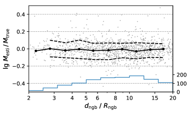
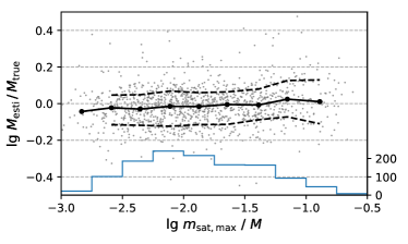
Figure 10: Influence of a massive neighbor (upper panel) or satellite (lower panel) on the halo mass estimate. Halo mass estimates from the EAGLE DF in terms of $\lg M_{\mathrm{esti}}/M_{\mathrm{true}}$ are shown as gray dots. The histograms show the number of test halos in each bin. The solid and dashed black curves show the median and the $1\sigma$ interval of $\lg M_{\mathrm{esti}}/M_{\mathrm{true}}$ for each bin. The nearest more massive neighbor is characterized by the ratio between its distance $d_{\mathrm{ngb}}$ to the test halo and its virial radius $R_{\mathrm{ngb}}$. The most massive satellite is characterized by the ratio between its subhalo mass $m_{\mathrm{sat,max}}$ and the halo mass $M$. See text for details.

Appendix D Enhanced satellite disruption and uncertainty in hydrodynamics-based simulations

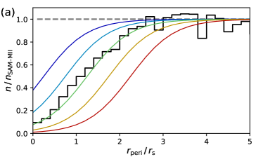
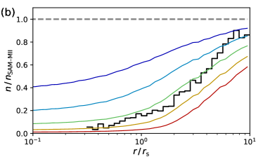
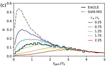
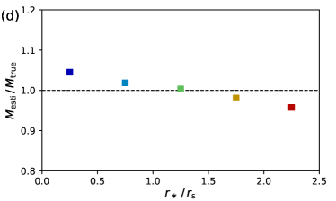
Figure 11: Influence of enhanced satellite disruption. The dashed gray and solid black curves represent the SAM-MII and EAGLE simulations, respectively, while the colored curves represent modified SAM-MII simulations with different enhancement of satellite disruption. (a) Ratio of the numbers of satellites in the modified and original SAM-MII simulations as a function of $r_{\mathrm{peri}}/r_{\mathrm{s}}$ for different enhanced disruption prescribed by $r_{\ast}$. The value of $r_{\ast}=1.25r_{\mathrm{s}}$ can approximately describe the EAGLE simulation. (b) Similar to (a) but for the radial distribution. (c) Similar to (a) but for the number of satellites as a function of $r_{\mathrm{peri}}/r_{\mathrm{s}}$. (d) Median mass estimates from modified SAM-MII DFs for mock observations of EAGLE halos.

While the hydrodynamics-based EAGLE simulation provides a better description of the observed MW satellite kinematics than the SAM-MII simulation, variation in treatment of physical processes in current hydrodynamics-based simulations also leads to scatter in the estimate of halo properties from the DF method. Here we estimate this scatter by mimicking enhanced satellite disruption in the SAM-MII simulation.

The central galaxy potential in hydrodynamics-based simulations can enhance satellite disruption in the inner halo, e.g., due to the enhancement of the tidal field by the stellar disk (e.g., Garrison-Kimmel et al., 2017; Kelley et al., 2019). We mimic this enhanced satellite disruption by manually removing a fraction $1-F_{\mathrm{surv}}$ of satellites from each SAM-MII template halo. Here

$$F_{\mathrm{surv}}=\frac{1}{1+\exp[2(r_{\ast}-r_{\mathrm{peri}})/r_{\mathrm{s}}]},$$ (D1)

$r_{\ast}$ is the characteristic pericenter distance for which half of the satellites are disrupted, and $r_{\mathrm{s}}$ is the characteristic radius of the NFW halo profile. Satellites with $r_{\mathrm{peri}}\gg r_{\ast}$ are not affected. We can mimic different enhancement of disruption by varying $r_{\ast}$, with $r_{\ast}=-\infty$ corresponding to no enhanced disruption and larger $r_{\ast}$ to more enhanced disruption. Modified distributions of satellites for various $r_{\ast}$ are shown as functions of $r_{\mathrm{peri}}$ and $r$ in Figure 11 (see Garrison-Kimmel et al. 2017 for similar figures). The distributions for the EAGLE simulation can be approximated by $r_{\ast}=1.25r_{\mathrm{s}}$. Comparing Figure 11 (b) and Figure 7 of Richings et al. (2020), we estimate $r_{\ast}\sim 0.25r_{\mathrm{s}}$ and $1.75r_{\mathrm{s}}$ for the APOSTLE and Auriga simulations, respectively. The central galaxies in the Auriga simulation are more massive and hence more efficient at disrupting satellites.

Using the modified SAM-MII satellite samples, we construct the corresponding DFs and apply them to estimate halo properties with mock observations of EAGLE halos. The prior based on the $M$-$c$ relation is used. Figure 11 (d) shows the dependence of the halo mass estimate on the enhancement of satellite disruption. As the $r_{\ast}$ for the modified SAM-MII DF changes from $1.25r_{\mathrm{s}}$ approximating the EAGLE simulation to $0.25r_{\mathrm{s}}$ ($1.75r_{\mathrm{s}}$) approximating the APOSTLE (Auriga) simulation, the resulting systematic bias in the halo mass estimate is $\lesssim 5\%$, which is negligible compared to the statistical uncertainty. This result is not surprising. Although the number of satellites changes due to different enhancement of disruption, their velocity distribution in the outer halo is less affected (e.g., Sawala et al., 2017; Richings et al., 2020). Because the halo mass estimate is mainly constrained by the velocity distribution rather than the spatial distribution (Li et al., 2019), this estimate is insensitive to the differences among hydrodynamics-based simulations. The above result is also consistent with the findings of Callingham et al. (2019), who recovered halo masses in the Auriga simulation with little bias using the orbital distribution from the EAGLE simulation.

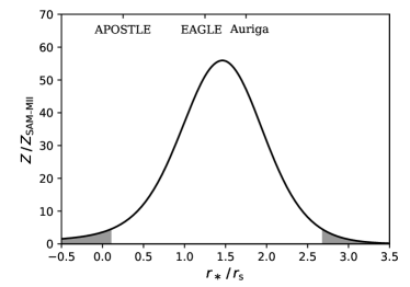
Figure 12: Constraints on enhanced satellite disruption from the observed MW satellite kinematics. The Bayesian factor of the modified relative to the original SAM-MII DF is shown as a function of $r_{\ast}/r_{\mathrm{s}}$. Values of $r_{\ast}/r_{\mathrm{s}}$ disfavored at the $2\sigma$ level are indicated by the gray shades. Approximate values of $r_{\ast}/r_{\mathrm{s}}$ for the hydrodynamics-based APOSTLE, EAGLE, and Auriga simulations are also indicated.

We calculate the Bayesian evidence of the modified SAM-MII DFs for the observed MW satellite kinematics. The results are shown in Figure 12. The DF with $r_{\ast}=1.5r_{\mathrm{s}}$ is the most favored. The corresponding projected DF $p_{\mathrm{s}}(r,v_{\mathrm{t}})$ is shown in Figure 7, and indeed matches the observations very well. The values of $r_{\ast}$ approximating the hydrodyanmics-based APOSTLE, EAGLE, and Auriga simulation suites are indicated in Figure 12. It can be seen that all three simulations are allowed by the current observations, though the APOSTLE results seem less favored (see also Riley et al. 2019). Clearly, the above comparison of these simulations is indirect and approximate. In the future, more actual simulations should be used to evaluate their Bayesian evidence as done for the EAGLE simulation in this study. For more precise comparison of the simulations, it helps to have a larger sample of MW satellites with more accurate data or a stacked sample of galaxy groups or clusters.

References

- Ablimit & Zhao (2017) Ablimit, I., & Zhao, G. 2017, ApJ, 846, 10
- Adén et al. (2009) Adén, D., Feltzing, S., Koch, A., et al. 2009, A&A, 506, 1147
- Astropy Collaboration et al. (2013) Astropy Collaboration, Robitaille, T. P., Tollerud, E. J., et al. 2013, A&A, 558, A33
- Bechtol et al. (2015) Bechtol, K., Drlica-Wagner, A., Balbinot, E., et al. 2015, ApJ, 807, 50
- Bellazzini et al. (2002) Bellazzini, M., Ferraro, F. R., Origlia, L., et al. 2002, AJ, 124, 3222
- Bellazzini et al. (2005) Bellazzini, M., Gennari, N., & Ferraro, F. R. 2005, MNRAS, 360, 185
- Binney & Wong (2017) Binney, J., & Wong, L. K. 2017, MNRAS, 467, 2446
- Bird et al. (2019) Bird, S. A., Xue, X.-X., Liu, C., et al. 2019, AJ, 157, 104
- Bland-Hawthorn & Gerhard (2016) Bland-Hawthorn, J., & Gerhard, O. 2016, ARA&A, 54, 529
- Boettcher et al. (2013) Boettcher, E., Willman, B., Fadely, R., et al. 2013, AJ, 146, 94
- Bonanos et al. (2004) Bonanos, A. Z., Stanek, K. Z., Szentgyorgyi, A. H., Sasselov, D. D., & Bakos, G. Á. 2004, AJ, 127, 861
- Bovy et al. (2010) Bovy, J., Murray, I., & Hogg, D. W. 2010, ApJ, 711, 1157
- Boylan-Kolchin et al. (2009) Boylan-Kolchin, M., Springel, V., White, S. D. M., Jenkins, A., & Lemson, G. 2009, MNRAS, 398, 1150
- Bressan et al. (2012) Bressan, A., Marigo, P., Girardi, L., et al. 2012, MNRAS, 427, 127
- Caldwell et al. (2017) Caldwell, N., Walker, M. G., Mateo, M., et al. 2017, ApJ, 839, 20
- Callingham et al. (2019) Callingham, T. M., Cautun, M., Deason, A. J., et al. 2019, MNRAS, 484, 5453
- Cautun et al. (2015) Cautun, M., Bose, S., Frenk, C. S., et al. 2015, MNRAS, 452, 3838
- Cautun & Frenk (2017) Cautun, M., & Frenk, C. S. 2017, MNRAS, 468, L41
- Cautun et al. (2019) Cautun, M., Benitez-Llambay, A., Deason, A. J., et al. 2019, arXiv:1911.04557
- Chabrier (2001) Chabrier, G. 2001, ApJ, 554, 1274
- Collins et al. (2017) Collins, M. L. M., Tollerud, E. J., Sand, D. J., et al. 2017, MNRAS, 467, 573
- Crain et al. (2015) Crain, R. A., Schaye, J., Bower, R. G., et al. 2015, MNRAS, 450, 1937
- Cuddeford (1991) Cuddeford, P. 1991, MNRAS, 253, 414
- Dall’Ora et al. (2006) Dall’Ora, M., Clementini, G., Kinemuchi, K., et al. 2006, ApJ, 653, L109
- Dall’Ora et al. (2012) Dall’Ora, M., Kinemuchi, K., Ripepi, V., et al. 2012, ApJ, 752, 42
- Deason et al. (2012) Deason, A. J., Belokurov, V., Evans, N. W., & An, J. 2012, MNRAS, 424, L44
- Deason et al. (2019) Deason, A. J., Fattahi, A., Belokurov, V., et al. 2019, MNRAS, 485, 3514
- Dutton & Macciò (2014) Dutton, A. A., & Macciò, A. V. 2014, MNRAS, 441, 3359
- Eadie & Jurić (2019) Eadie, G., & Jurić, M. 2019, ApJ, 875, 159
- Erkal et al. (2020) Erkal, D., Belokurov, V., & Parkin, D. L. 2020, arXiv:2001.11030
- Evans & An (2006) Evans, N. W., & An, J. H. 2006, Phys. Rev. D, 73, 023524
- Fritz et al. (2018) Fritz, T. K., Battaglia, G., Pawlowski, M. S., et al. 2018, A&A, 619, A103
- Fritz et al. (2019) Fritz, T. K., Carrera, R., Battaglia, G., & Taibi, S. 2019, A&A, 623, A129
- Fritz et al. (2020) Fritz, T. K., Di Cintio, A., Battaglia, G., Brook, C., & Taibi, S. 2020, arXiv:2001.02651
- Gaia Collaboration et al. (2018a) Gaia Collaboration, Brown, A. G. A., Vallenari, A., et al. 2018a, A&A, 616, A1
- Gaia Collaboration et al. (2018b) Gaia Collaboration, Helmi, A., van Leeuwen, F., et al. 2018b, A&A, 616, A12
- Garofalo et al. (2013) Garofalo, A., Cusano, F., Clementini, G., et al. 2013, ApJ, 767, 62
- Garrison-Kimmel et al. (2017) Garrison-Kimmel, S., Wetzel, A., Bullock, J. S., et al. 2017, MNRAS, 471, 1709
- Grand et al. (2019) Grand, R. J. J., Deason, A. J., White, S. D. M., et al. 2019, MNRAS, 487, L72
- Greco et al. (2008) Greco, C., Dall’Ora, M., Clementini, G., et al. 2008, ApJ, 675, L73
- Guo et al. (2011) Guo, Q., White, S., Boylan-Kolchin, M., et al. 2011, MNRAS, 413, 101
- Han et al. (2016a) Han, J., Wang, W., Cole, S., & Frenk, C. S. 2016a, MNRAS, 456, 1017
- Han et al. (2016b) —. 2016b, MNRAS, 456, 1003
- Han et al. (2019) Han, J., Wang, W., & Li, Z. 2019, arXiv:1909.02690
- Huang et al. (2016) Huang, Y., Liu, X. W., Yuan, H. B., et al. 2016, MNRAS, 463, 2623
- Hubert et al. (2018) Hubert, M., Debruyne, M., & Rousseeuw, P. J. 2018, Wiley Interdisciplinary Reviews: Computational Statistics, 10, e1421
- Hunter (2007) Hunter, J. D. 2007, CSE, 9, 90
- Jethwa et al. (2016) Jethwa, P., Erkal, D., & Belokurov, V. 2016, MNRAS, 461, 2212
- Jing (2000) Jing, Y. P. 2000, ApJ, 535, 30
- Kafle et al. (2014) Kafle, P. R., Sharma, S., Lewis, G. F., & Bland-Hawthorn, J. 2014, ApJ, 794, 59
- Kallivayalil et al. (2018) Kallivayalil, N., Sales, L. V., Zivick, P., et al. 2018, ApJ, 867, 19
- Karczmarek et al. (2015) Karczmarek, P., Pietrzyński, G., Gieren, W., et al. 2015, AJ, 150, 90
- Kelley et al. (2019) Kelley, T., Bullock, J. S., Garrison-Kimmel, S., et al. 2019, MNRAS, 487, 4409
- Kirby et al. (2013) Kirby, E. N., Boylan-Kolchin, M., Cohen, J. G., et al. 2013, ApJ, 770, 16
- Kirby et al. (2015) Kirby, E. N., Simon, J. D., & Cohen, J. G. 2015, ApJ, 810, 56
- Kochanek (1996) Kochanek, C. S. 1996, ApJ, 457, 228
- Koposov et al. (2008) Koposov, S., Belokurov, V., Evans, N. W., et al. 2008, ApJ, 686, 279
- Koposov et al. (2015a) Koposov, S. E., Belokurov, V., Torrealba, G., & Evans, N. W. 2015a, ApJ, 805, 130
- Koposov et al. (2011) Koposov, S. E., Gilmore, G., Walker, M. G., et al. 2011, ApJ, 736, 146
- Koposov et al. (2015b) Koposov, S. E., Casey, A. R., Belokurov, V., et al. 2015b, ApJ, 811, 62
- Kuehn et al. (2008) Kuehn, C., Kinemuchi, K., Ripepi, V., et al. 2008, ApJ, 674, L81
- Li et al. (2017) Li, Z.-Z., Jing, Y. P., Qian, Y.-Z., Yuan, Z., & Zhao, D.-H. 2017, ApJ, 850, 116
- Li et al. (2019) Li, Z.-Z., Qian, Y.-Z., Han, J., Wang, W., & Jing, Y. P. 2019, ApJ, 886, 69
- Little & Tremaine (1987) Little, B., & Tremaine, S. 1987, ApJ, 320, 493
- Loebman et al. (2018) Loebman, S. R., Valluri, M., Hattori, K., et al. 2018, ApJ, 853, 196
- Longeard et al. (2020) Longeard, N., Martin, N., Starkenburg, E., et al. 2020, MNRAS, 491, 356
- Lynden-Bell (1967) Lynden-Bell, D. 1967, MNRAS, 136, 101
- Magorrian (2014) Magorrian, J. 2014, MNRAS, 437, 2230
- Martin et al. (2008) Martin, N. F., de Jong, J. T. A., & Rix, H.-W. 2008, ApJ, 684, 1075
- Martin et al. (2015) Martin, N. F., Nidever, D. L., Besla, G., et al. 2015, ApJ, 804, L5
- Martínez-Vázquez et al. (2015) Martínez-Vázquez, C. E., Monelli, M., Bono, G., et al. 2015, MNRAS, 454, 1509
- Massari & Helmi (2018) Massari, D., & Helmi, A. 2018, A&A, 620, A155
- Mateo et al. (2008) Mateo, M., Olszewski, E. W., & Walker, M. G. 2008, ApJ, 675, 201
- McAlpine et al. (2016) McAlpine, S., Helly, J. C., Schaller, M., et al. 2016, A&C, 15, 72
- McConnachie (2012) McConnachie, A. W. 2012, AJ, 144, 4
- McMillan (2011) McMillan, P. J. 2011, MNRAS, 414, 2446
- McMillan (2017) —. 2017, MNRAS, 465, 76
- McMonigal et al. (2014) McMonigal, B., Bate, N. F., Lewis, G. F., et al. 2014, MNRAS, 444, 3139
- Medina et al. (2017) Medina, G. E., Muñoz, R. R., Vivas, A. K., et al. 2017, ApJ, 845, L10
- Moretti et al. (2009) Moretti, M. I., Dall’Ora, M., Ripepi, V., et al. 2009, ApJ, 699, L125
- Muñoz et al. (2010) Muñoz, R. R., Geha, M., & Willman, B. 2010, AJ, 140, 138
- Musella et al. (2009) Musella, I., Ripepi, V., Clementini, G., et al. 2009, ApJ, 695, L83
- Musella et al. (2012) Musella, I., Ripepi, V., Marconi, M., et al. 2012, ApJ, 756, 121
- Navarro et al. (1996) Navarro, J. F., Frenk, C. S., & White, S. D. M. 1996, ApJ, 462, 563
- Nesti & Salucci (2013) Nesti, F., & Salucci, P. 2013, J. Cosmology Astropart. Phys, 2013, 016
- Newton et al. (2018) Newton, O., Cautun, M., Jenkins, A., Frenk, C. S., & Helly, J. C. 2018, MNRAS, 479, 2853
- Okamoto et al. (2017) Okamoto, S., Arimoto, N., Tolstoy, E., et al. 2017, MNRAS, 467, 208
- Oliphant (2007) Oliphant, T. E. 2007, CSE, 9, 10
- Pace & Li (2019) Pace, A. B., & Li, T. S. 2019, ApJ, 875, 77
- Pardy et al. (2020) Pardy, S. A., D’Onghia, E., Navarro, J. F., et al. 2020, MNRAS, 492, 1543
- Patel et al. (2018) Patel, E., Besla, G., Mandel, K., & Sohn, S. T. 2018, ApJ, 857, 78
- Pawlowski & Kroupa (2013) Pawlowski, M. S., & Kroupa, P. 2013, MNRAS, 435, 2116
- Peñarrubia & Fattahi (2017) Peñarrubia, J., & Fattahi, A. 2017, MNRAS, 468, 1300
- Peñarrubia et al. (2016) Peñarrubia, J., Gómez, F. A., Besla, G., Erkal, D., & Ma, Y.-Z. 2016, MNRAS, 456, L54
- Pedregosa et al. (2012) Pedregosa, F., Varoquaux, G., Gramfort, A., et al. 2012, arXiv:1201.0490
- Petersen & Peñarrubia (2020) Petersen, M. S., & Peñarrubia, J. 2020, MNRAS, 494, L11
- Pietrzyński et al. (2009) Pietrzyński, G., Górski, M., Gieren, W., et al. 2009, AJ, 138, 459
- Posti et al. (2015) Posti, L., Binney, J., Nipoti, C., & Ciotti, L. 2015, MNRAS, 447, 3060
- Posti & Helmi (2019) Posti, L., & Helmi, A. 2019, A&A, 621, A56
- Richings et al. (2020) Richings, J., Frenk, C., Jenkins, A., et al. 2020, MNRAS, 492, 5780
- Riley et al. (2019) Riley, A. H., Fattahi, A., Pace, A. B., et al. 2019, MNRAS, 486, 2679
- Sakamoto et al. (2003) Sakamoto, T., Chiba, M., & Beers, T. C. 2003, A&A, 397, 899
- Sand et al. (2012) Sand, D. J., Strader, J., Willman, B., et al. 2012, ApJ, 756, 79
- Sawala et al. (2017) Sawala, T., Pihajoki, P., Johansson, P. H., et al. 2017, MNRAS, 467, 4383
- Schaller et al. (2015) Schaller, M., Frenk, C. S., Bower, R. G., et al. 2015, MNRAS, 451, 1247
- Schaye et al. (2015) Schaye, J., Crain, R. A., Bower, R. G., et al. 2015, MNRAS, 446, 521
- Shao et al. (2019) Shao, S., Cautun, M., & Frenk, C. S. 2019, MNRAS, 488, 1166
- Simon (2018) Simon, J. D. 2018, ApJ, 863, 89
- Simon (2019) —. 2019, ARA&A, 57, 375
- Simon & Geha (2007) Simon, J. D., & Geha, M. 2007, ApJ, 670, 313
- Simon et al. (2019) Simon, J. D., Li, T. S., Erkal, D., et al. 2019, arXiv:1911.08493
- Sohn et al. (2018) Sohn, S. T., Watkins, L. L., Fardal, M. A., et al. 2018, ApJ, 862, 52
- Spencer et al. (2017) Spencer, M. E., Mateo, M., Walker, M. G., & Olszewski, E. W. 2017, ApJ, 836, 202
- Stetson et al. (2014) Stetson, P. B., Fiorentino, G., Bono, G., et al. 2014, PASP, 126, 616
- Torrealba et al. (2016a) Torrealba, G., Koposov, S. E., Belokurov, V., & Irwin, M. 2016a, MNRAS, 459, 2370
- Torrealba et al. (2016b) Torrealba, G., Koposov, S. E., Belokurov, V., et al. 2016b, MNRAS, 463, 712
- Torrealba et al. (2019) Torrealba, G., Belokurov, V., Koposov, S. E., et al. 2019, MNRAS, 488, 2743
- Trotta (2008) Trotta, R. 2008, ConPh, 49, 71
- van der Walt et al. (2011) van der Walt, S., Colbert, S. C., & Varoquaux, G. 2011, CSE, 13, 22
- Vasiliev (2019) Vasiliev, E. 2019, MNRAS, 484, 2832
- Vivas et al. (2016) Vivas, A. K., Olsen, K., Blum, R., et al. 2016, AJ, 151, 118
- Walker et al. (2009) Walker, M. G., Mateo, M., & Olszewski, E. W. 2009, AJ, 137, 3100
- Walker et al. (2015) Walker, M. G., Olszewski, E. W., & Mateo, M. 2015, MNRAS, 448, 2717
- Walker et al. (2016) Walker, M. G., Mateo, M., Olszewski, E. W., et al. 2016, ApJ, 819, 53
- Walsh et al. (2009) Walsh, S. M., Willman, B., & Jerjen, H. 2009, AJ, 137, 450
- Wang et al. (2019) Wang, W., Han, J., Cautun, M., Li, Z., & Ishigaki, M. N. 2019, arXiv:1912.02599
- Wang et al. (2017) Wang, W., Han, J., Cole, S., Frenk, C., & Sawala, T. 2017, MNRAS, 470, 2351
- Wang et al. (2018) Wang, W., Han, J., Cole, S., et al. 2018, MNRAS, 476, 5669
- Wang et al. (2015) Wang, W., Han, J., Cooper, A. P., et al. 2015, MNRAS, 453, 377
- Watkins et al. (2010) Watkins, L. L., Evans, N. W., & An, J. H. 2010, MNRAS, 406, 264
- Watkins et al. (2019) Watkins, L. L., van der Marel, R. P., Sohn, S. T., & Evans, N. W. 2019, ApJ, 873, 118
- Wilkinson & Evans (1999) Wilkinson, M. I., & Evans, N. W. 1999, MNRAS, 310, 645
- Williams & Evans (2015a) Williams, A. A., & Evans, N. W. 2015a, MNRAS, 454, 698
- Williams & Evans (2015b) —. 2015b, MNRAS, 448, 1360
- Willman et al. (2011) Willman, B., Geha, M., Strader, J., et al. 2011, AJ, 142, 128
- Wojtak et al. (2008) Wojtak, R., Łokas, E. L., Mamon, G. A., et al. 2008, MNRAS, 388, 815
- Xue et al. (2008) Xue, X. X., Rix, H. W., Zhao, G., et al. 2008, ApJ, 684, 1143
- Zaritsky et al. (2020) Zaritsky, D., Conroy, C., Zhang, H., et al. 2020, ApJ, 888, 114
- Zhai et al. (2018) Zhai, M., Xue, X.-X., Zhang, L., et al. 2018, RAA, 18, 113